Visualized Wave Mechanics by Coupled Macroscopic Pendula: Classical Analogue to Driven Quantum Bits
Abstract
Quantum mechanics increasingly penetrates modern technologies but, due to its non-deterministic nature seemingly contradicting our classical everyday world, our comprehension often stays elusive. Arguing along the correspondence principle, classical mechanics is often seen as a theory for large systems where quantum coherence is completely averaged out. Surprisingly, it is still possible to reconstruct the coherent dynamics of a quantum bit (qubit) by using a classical model system. This classical-to-quantum analogue is based on wave mechanics, which applies to both, the classical and the quantum world. In this spirit we investigate the dynamics of macroscopic physical pendula with a modulated coupling. As a proof of principle, we demonstrate full control of our one-to-one analogue to a qubit by realizing Rabi oscillations, Landau-Zener (LZ) transitions and Landau-Zener-Stückelberg-Majorana (LZSM) interferometry. Our classical qubit demonstrator can help comprehending and developing useful quantum technologies.
Quantum technology already has a drastic impact on society. This development presently accelerates with our growing ability to harvest coherent quantum dynamics for engineering game changing devices such as quantum computers or a quantum internet. At the same time, while the mathematical framework of quantum mechanics can be considered complete, fundamental aspects of the underlying physics, even on the level of only few qubits are outside our empirical world. In this situation, classical model systems capable of enlightening the often elusive coherent dynamics of quantum systems may prove very useful Shore et al. 2009. This approach might be fundamentally questioned due to a central paradigm of quantum dynamics, which is its probabilistic nature in contrast to the deterministic classical equation of motion (EOM). Nevertheless, besides non-determinism and non-locality, wave properties and the superposition principle being central elements of quantum mechanics appear also in classical physics. For example, the quantum mechanical double split experiment may be visualized with classical water waves. Here we visualize one of the most basic quantum systems, a qubit, by physical macroscopic pendula.
Classical dynamics can generally be formulated in terms of second-order, non-linear and inhomogeneous differential equations, while non relativistic quantum mechanics is based on the first order, homogeneous and linear Schrödinger equation. Hence, most classical systems are improper for simulating qubit dynamics. In this article, we derive the conditions under which classical pendula with modulated coupling nevertheless can be described by a Schrödinger-like equation. We demonstrate this classical-to-quantum analogue by exploring three realizations of qubit control, namely Rabi oscillations Rabi 1937, LZ transitions Landau 1932; Zener 1932 and, finally, LZSM interferometry Stueckelberg 1932; Majorana 1932.
Recent developments in quantum technology have motivated theoretical Shore et al. 2009; Grønbech-Jensen and Cirillo 2005; Novotny 2010; Heinrich et al. 2010; Frimmer and Novotny 2014; Ivakhnenko et al. 2018; Parafilo and Kiselev 2018 and experimental Süsstrunk and Huber 2015; Nash et al. 2015; Faust et al. 2013; Seitner et al. 2016 projects exploring analogues between classical coupled oscillators and its quantum version. The most interesting dynamics happens at avoided crossings of the eigenmodes of coupled oscillators near resonance. Previous theoretical considerations Novotny 2010; Frimmer and Novotny 2014; Ivakhnenko et al. 2018 and experiments Faust et al. 2013; Seitner et al. 2016 with nanomechanical oscillators used a time-dependent frequency difference corresponding to the detuning usually modulated in case of qubits Mullen et al. 1989; Vitanov 1999; Wubs et al. 2005; Sillanpää et al. 2005; Berns et al. 2008; Stehlik et al. 2012; Forster et al. 2014; Forster et al. 2015; Heinrich et al. 2021. To experimentally establish a classical-to-quantum analogue based on macroscopic pendula we instead modulate the coupling, which for this system is more practical than driving the detuning. This gimmick, for the first time allows us to continuously monitor the coherent dynamics of a driven two-level system at ambient conditions and to observe it with bare eyes. As we establish a one-to-one correspondence, our coupled pendula directly visualize the coherent dynamics of a driven qubit.
Setup and model

In Fig. 1 we display a photograph and a simplified sketch of the setup. It consists of two pendula, each being described by its deflection angle and its angular frequency with . The two pendula are coupled via permanent magnets and detuned by the frequency difference . To probe the dynamics of qubits, usually the energy detuning between the diabatic states is modulated. However, modulating the coupling is mathematically equivalent after applying the appropriate basis transformation. For our system it is more practical to modulate the coupling. For this purpose we employ a battery driven linear motor, which rotates one of the magnets around the axis defined by the pendulum rod. As a result, the coupling and, at the same time, the equilibrium deflections of the pendula, , are periodically modulated in time. The latter correspond to the quasistatic solution of the driven system, describing the (momentary) adiabatic equilibrium position.
We consider the deviation from the adiabatic equilibrium, . Aiming at a description in the form of a Schrödinger equation, which is linear and of first order, experiments and theory have to facilitate a linearization of the non-linear Newton EOM. This requires small deflection angles, small frequency differences and similar moments of inertia of the uncoupled pendula. The linearized version of the EOM reads
| (1) |
where is the average pendulum (angular) frequency and is the coupling in units of frequency 11 1 In the interaction term, we have neglected the small difference of the moments of interia. Moreover, the sign of is chosen such that it matches the usual definition in the quantum mechanical two-level problem. It is positive for attractive interaction.. The symmetry of the interaction terms on the right-hand side of Eq. (1) is essential for resembling the Schrödinger equation and requires neglecting the difference between the moments of inertia. Our modulated coupling, , corresponds to the time-dependent level detuning commonly used to drive qubits, for instance in the context of the quantum mechanical LZSM problem Shevchenko et al. 2010; Ivakhnenko et al. 2023. To simplify a comparison with typical qubit experiments we aim at a coupling of the common form , which renders Eq. (1) a Mathieu equation Mathieu 1868. This modulation requires an experimental setup allowing for the far-field approximation of the dipole-dipole interaction.
For simulating qubit experiments we would like to independently modify the mean coupling and the modulation amplitude . To achieve this, we use two sets of magnet pairs, see Fig. 1. The lower magnets are attached at the distance from the pivots and the upper magnets at , where is sufficiently large to allow us to neglect quadrupole components of the coupling. The coupling is then composed of the sum of the contributions of the upper versus lower magnets, , where we slowly modulate by rotating one of the lower magnets. The time-dependence of the reference point of the linearization, , leads to harmonic mixing such that aquires a contribution from the rotating magnets and, vice versa, is also affected by the static magnets.
The linearized EOM Eq. (1), which is still of second order, describes the free oscillations of two pendula with modulated coupling. In comparison, the Schrödinger equation of a qubit describes probability functions. These correspond to the slowly varying occupation amplitudes of the two pendula, given by the envelope functions, say , of the individual rapid oscillations . To separate the time scales, we therefore employ the ansatz
| (2) |
with a rapidly oscillating prefactor and slowly varying complex envelopes . Inserting the ansatz into Eq. (1), while neglecting second order derivatives of , we find
| (3) |
which for possesses the form of a Schrödinger equation of the driven two-level system in the representation frequently found in textbooks for the Rabi problem (in a gauge without in the diagonal).
For describing LZ transitions of a qubit with time-dependent detuning one usually uses the diabatic basis, in which the constant tunnel coupling appears in the off-diagonal matrix elements of the Hamiltonian. As we modulate the coupling between our pendula, it is convenient to transform into the according diabatic basis of the in-phase and out-of-phase modes, , in which the constant frequency difference appears in the off-diagonal elements of the Hamiltonian. With defined in accordance with Eq. (2) the presentation of the LZ problem for our pendula then reads
| (4) |
Equations (3) and (4) provide the foundation for comparing the dynamics of classical pendula with that of a qubit. They describe the occupation amplitudes of our coupled pendula in the form of a Schrödinger equation in the two alternative bases versus . In Appendices A and B we offer an elegant alternative derivation based on the Lagrange formulation of classical mechanics and starting from the non-linear Newton equation. We also demonstrate there, how the time-dependent quasi static equilibrium, , contributes to the static and discuss limitations of our approximations.
In a nutshell, Eq. (3) describes —for the case of a time dependent coupling between the pendula— the dynamics of the occupation amplitudes of the individual pendula. In this way, the eigenmodes of the uncoupled pendula directly correspond to the wave functions of the localized sates of a qubit. Equation (3) is the natural choice for predicting Rabi oscillations occurring between the occupation amplitudes of the individual pendula for weak coupling. A basis transformation yields Eq. (4), which describes the dynamics between the occupation amplitudes of the in-phase and out-of-phase superposition modes of the individual pendula. Without driving, they resemble the eigenmodes of two strongly coupled pendula and correspond to the eigenfunctions of a qubit at zero detuning. Consequently, Eq. (4) is the natural choice for predicting the dynamics of the occupation amplitudes in the regime of LZ transitions, where the maximum coupling exceeds the detuning. See Appendix B.3 and Table 1 therein for a one-to-one comparison between the parameters of a qubit and the pendula.
In our experiments we control and by varying the distance between the lower magnets, corresponding to the distance between the pivots, and optionally the distance between the upper magnets [positioned inside the red horizontal cylindric housings seen in Fig. 1(a)], both defined for . In addition, we adjust the frequency difference, , by moving a heavy weight [vertical brass cylinders partly visible in Fig. 1(a)] using a standard thread along one of the pendulum rods. We employ a line scan camera to simultaneously image at a rate of 10 Hz the lateral positions of both pendula within a linear pixel array. Applying numerical filtering we then obtain the displacement angles as a function of time, see Appendix E. The mean frequency of our pendula is close to Hz. To ensure the validity of the linearized Eq. (1), we work with small deflections , modulation frequencies and frequency differences . Thereby is always the largest frequency by far supporting the separation of time scales in Eq. (2). The quality factor of of the coupled pendula is high enough to allow us ignoring dissipation as we did in the model above. In order to achieve high and stable quality factors, we employ professional pendulum clock pivots based on leaf springs provided by the company Erwin Sattler GmbH & Co. KG. In detail our experimental results indicate, that the damping of the coupled pendula motion is dominated by magnetic induction, i.e., eddy currents induced inside the conducting magnets due to their relative motion. The friction of air and the deforming pivot springs dominate the damping of the uncoupled pendula with stable quality factors of . Note, that we can easily achieve the strong coupling regime as our maximal coupling of Hz exceeds the resonance line width of Hz by more than three orders of magnitude.
Analysis and Discussion
To explore the analogy between our coupled pendula and a qubit we first perform Rabi oscillations between the individual pendula in the limit of fast driving with , where the driving amplitude becomes the Rabi frequency, . After that, we turn to “qubit manipulation” using LZ transitions between the superposition modes, , in the limit of slow driving, .

we present Rabi oscillations for two different pivot distances but otherwise identical conditions. We use no upper magnets and weak couplings (large ), such that and . Shown are the deflections in respect to the equilibrium . The observed beatings between the pendula are Rabi oscillations, where the variation between Rabi frequencies in Fig. 2(a) versus Fig. 2(b) reflect the differences in . In both cases the energy transfer between the pendula is almost complete, as we chose a near resonance condition . Small steps, which occur at the repetition rate [zoom into Figs. 2(a) and 2(b) to clearly see them], indicate side band transitions beyond the rotating wave approximation. In Fig. 2(b) these steps are bigger due to a larger modulation amplitude compared to Fig. 2(a).
By varying we next explore the Rabi dynamics near resonance. In Fig. 2(c) we present the effective Rabi frequency corresponding to the actual beating frequency. Likewise, in Fig. 2(d) we show the visibility defined as the fraction of energy exchanged between the pendula. Symbols are measured data while the lines visualize the theory predictions, and . The only fit parameter is the Rabi frequency mHz, which defines the minimum of at resonance and which can be used to accurately determine the magnetic moment , see Appendix C. The excellent agreement between theory and experiment underlines the high quality of our classical mechanics experiment. Since the model curves can be derived from the Schrödinger equation (3), the result establishes a first analogue between classical pendula and a qubit.
An elegant method to manipulate qubits in the limit of slow modulation, , are LZ transitions Saito et al. 2006; Ribeiro and Burkard 2009. In Fig. 3(a)
we present the deflection angles , while one of the magnets completes one full rotation. Within this driving period, the pendula pass twice through the avoided crossing at zero coupling, sketched in Fig. 3(d), namely from positive to negative and back. At , we initialized , such that . This is evident in Fig. 3(b) plotting the in-phase and out-of-phase combinations . In Fig. 3(c) we present the according populations , given by the square modulus of the slowly varying amplitude, , normalized such that . Around the two avoided crossings (indicated by vertical dotted lines) we observe LZ transitions. The first one, which mixes and , is followed by beats with the time dependent frequency clearly visible between and as well as between and . The latter beats confirm theoretical predictions Mullen et al. 1989; Vitanov 1999; Wubs et al. 2005, namely chirped oscillations centered around the LZ probability and , respectively, right after passing through the avoided crossing. Here, is the sweep velocity at , which depends on , and . This observation demonstrates an advantage of our classical two-level system, which—in contrast to a qubit—allows us to trace the time evolution of population probabilities in real time in a single shot measurement. Based on the comparison with theory, we identify the long-time transition probability of a single LZ transition by averaging out the beats of the measured occupation within an appropriate time window after half of the modulation period , i.e., centered between the two LZ transitions. In Fig. 3(e) we compare the resulting for a wide range of the parameters , , and with the classic result for the limit Landau 1932; Zener 1932; Stueckelberg 1932; Majorana 1932.
The agreement between model and measurements is good albeit compared to the Rabi experiment above the data scatter considerably around the model line. These deviations can be explained with the initialization into at finite , which for is not an eigenmode, as it would be for an initialization at Landau 1932; Zener 1932. The weak admixture of the second eigenmode gives rise to a weak beating between right after initialization as visible in Fig. 3(b) for min. Treating the relative phase between the modes (which could be predetermined at the cost of additional experimental effort) as an unknown, we predict the range of possible values of for arbitrary phases [gray area in Fig. 3(e)]. In the adiabatic limit, , independent of the relative phase the finite occupation of the upper eigenmode, , results in while .
Note, that in a corresponding experiment with an actual qubit the initialization procedure would be similar, such that the phase problem described above occurs as well. However, only the classical qubit analog allowed us to perform continuous measurements as those in Fig. 3(c), which helped us to fully determine the influence of the non-zero phase at initialization. This result is an example of the usefulness of our classical approach for deciphering the sometimes complex dynamics of qubits.
Each LZ transition mixes the eigenmodes as demonstrated in Fig. 3(e). The resulting superposition state then accumulates the adiabatic phase integrating the difference between the two eigenfrequencies with the Stokes phase added Shevchenko et al. 2010. The second LZ transition is then heavily influenced by these phases Stueckelberg 1932; Majorana 1932. Indeed, multiple LZ transitions result in a complicated time evolution of as can be seen in Fig. 4(a),

which presents two example time traces of . While the modulation frequency is identical for both measurements, mHz, we varied and . Each trace covers five modulation periods corresponding to ten LZ transitions. Most of them are clearly visible as more or less pronounced steps while for some transitions stays almost unchanged beyond the perpetual beating. The steady state solution for continuous driving averaging over many periods gives rise to LZSM interference patterns , which can be used for exploring qubit dynamics, decoherence or multi-color driving Forster et al. 2014; Forster et al. 2015. For a practical comparison, allowing for small deviations, we average over the initial five modulation periods. In Fig. 4(b) we present the LZSM interference pattern as a gray scale, which we computed using the Schrödinger equation (4). In Figs. 4(c) and 4(d) we finally present interference traces along the two solid lines in Fig. 4(b), mind the color code. In Fig. 4(c) we plot for the case without upper magnets, while for Fig. 4(d) we added the upper magnets and show for a constant pivot distance, mm. Solid lines are model curves calculated with Eq. (4) [contained in the gray scale plot in Fig. 4(b)], while the dots present measured interference patterns. Hereby, each point corresponds to the average of a trace as those shown in Fig. 4(a). Our measurements qualitatively reproduce the calculated interference fringes. Quantitative deviations indicate the limitations of the mapping of the Newton equation onto the Schrödinger equation, in particular for large and . In Appendix D we provide related background information.
Summary
Wave mechanics introduced by Erwin Schrödinger in 1926 Schrödinger 1926 provides a mathematical description for the coherent dynamics of a qubit. However, a continuous experimental visualization of its time evolution is hindered by the principle of projection measurement; each measurement would destroy the quantum coherence. In comparison, our classical qubit analog surely allows to trace the complete time evolution in a single measurement. In order to actually visualize Schrödingers wave mechanics using physical pendula with modulated coupling one has to map the non-linear, second order and inhomogeneous classical EOM to the linear, first order and homogeneous Schrödinger equation. This mapping, which includes a linearization, a rotating wave approximation and a time-dependent shift of the reference point, also clarifies the experimental conditions necessary for classical qubit simulator experiments and their physical interpretations. In this spirit, we presented three key qubit experiments with coupled pendula, namely Rabi oscillations, LZ transitions and LZSM interferometry. Comparing measurements with the prediction of the Schrödinger equation we demonstrated that our classical experiments directly visualize Schrödinger’s wave mechanics. Our classical qubit simulator bridges the gap between the elusiveness of quantum mechanics and the common imagination pre-shaped by classical experiences. The experimental setup is highly versatile and might be used for exploring a variety of phenomena beyond simulating a qubit, such as geometrical phases Berry 1984, after adding more pendula, multi-level systems Mi et al. 2018; Shevchenko et al. 2018 or coherent transfer by adiabatic passage Menchon-Enrich et al. 2016 or simulating the non-linear Schrödinger equation Leggett 2001. Moreover, driven systems of coupled pendula may serve as visualizer of a large variety of coupled systems in nature or even economical, social or financial systems. However, a limit to any classical model system is imposed by entanglement of multiple qubits, which has no classical analog.
Acknowledgements
The authors thank W. Kurpas and S. Manus for technical support. H.L. thanks K. Pfeffer and R. Buchholz for frequent discussions of the ongoing experiments. This work was financially supported by the Center for NanoScience (CeNS) at LMU Munich, by the Spanish Ministry of Science and Innovation through Grant. No. PID2020-117787GB-I00, the CSIC Research Platform on Quantum Technologies PTI-001 and the Institute for Basic Science in Korea (IBS-R024-D1). The work of M.K. is conducted within the framework of the Trieste Institute for Theoretical Quantum Technologies (TQT).
Author’s contributions
S.L. and M.K. initiated the project and planned it together with H.L. The experimental setup of the coupled pendula was designed by H.L. and S.L. H.L. performed the experiments. The data were analyzed by all authors. M.K. and S.K. formulated the theoretical model. S.K., M.K., and A.P. computed the theoretical data. S.K., M.K. and S.L. wrote the article including the appendices.
Appendix A Newton equation

To derive the equation of motion, we employ the Lagrange formalism. For two uncoupled physical pendula the Langrangian reads Goldstein et al. 2001
| (5) |
where labels the two so-far uncoupled pendula and the deflection angles are zero for vertically hanging pendula described by their moments of inertia . In the second term, which is the negative potential energy, we have already made use of the fact that the eigenfrequency reads , with the gravity acceleration , the mass , which is equal for both pendula, and the distance between the pivot and the center of mass of each pendulum. Note, that up to Eq. (19), denotes the deflection angles in the lab frame with the vertical direction as reference.
A.1 Coupling by magnets
The two pendula are coupled by either one or two pairs of permanent neodymium magnets as sketched in Fig. 5(a) for the case of one pair of magnets. The cubical magnets can be seen in the photograph in Fig. 5(b). Two large magnets with 28 mm edge lengths are fixed to the end of each rod and can be rotated by battery driven motors. Two smaller magnets are positioned inside the red cylinders 0.513 m above. All magnet cubes are magnetized along their horizontal four-fold axes, which at all times remain fixed within the oscillation plane with the excumption of one of the lower magnets optionally rotated around the rod it is attached to.
With the origin set to the pivot of the left pendulum (), the magnets have positions
| (6) |
where is the horizontal distance between the pivots of the pendula, and is the distance between magnet and pivot, which is equal for both pendula. Their magnetic dipole moments of identical magnitude are oriented as
| (7) |
valid for large enough as is the case in all our experiments.
The magnetic dipole-dipole coupling energy is Jackson 1999
| (8) |
where . To express this in terms of our dynamical variables , we insert the vectors in Eqs. (6) and (7) and obtain the potential energy of the coupling to read , where
| (9) |
Length and orientation of follow from straightforward geometric considerations and read
| (10) |
where is the angle between the -axis and , cf. Fig. 5. In some of our experiments, we use two pairs of magnets, i.e., a lower pair connected to the ends of the rods and an upper pair with a variable horizontal distance shifted upwards along the rods. Consequently, we introduce the respective distances (replacing ) and between pivots and lower versus upper magnets. Hereby, exceeds the horizontal distance roughly by a factor two, such that we can neglect the interaction between the upper and the lower magnets and consider two separate dipole-dipole couplings. The upper magnets orientations are fixed, such that their magnetizations are perpendicular to the respective rods, remain in the - plane and attract each other. In contrast, one of the lower magnets is rotated such that
| (11) |
The equations of motion follow readily from the Lagrange equation Goldstein et al. 2001
| (12) |
For the full Lagrangian, , they become
| (13) |
The derivative of the interaction potential is straightforward to calculate but results in a bulky expression, whose explicit form is not needed for our discussion. Equations (13) can be integrated numerically to obtain a full solution of the pendula dynamics which considers all nonlinearities.
A.2 Linearization and quasistatic solution
The mapping of Newton’s equation of motion to a Schrödinger equation requires a bilinear Lagrangian, as will become clear in Sec. B below. In our experiment, the deflection angles are rather small, , such that already a linearized version of the equation of motion provides a faithful description. We will perform this linearization by an expansion for the Lagrangian up to second order in . Then the Lagrangian of the uncoupled pendula, Eq. (5), takes the bilinear form , where we have omitted an irrelevant constant term. The expansion of the interaction term (9) requires more effort, because the appear in both the numerator and the denominator.
Closer inspection of the expressions, however, reveals that the -dependence of the numerator is much weaker than that of the denominator, given by , see Eq. (10). The difference stems from the numerical pre-factors of the second-order terms of the Taylor expansions of and , which are and , respectively. Moreover, in the are weighted by a factor , which for our experiment is . This leads to the conclusion that the numerator is responsible for only of the curvature of . Hence, we neglect the higher order terms of the numerator and approximate . However, we do consider the terms stemming from the expansion of the denominator,
| (14) |
with . Inserting the relevant terms up to second order into Eq. (9) yields the Langrangian of the linearized problem
| (15) |
For our two pairs of magnets, where one of the lower magnets is rotating, the energies and take the form
| (16) |
where the tilde indicates parameters stemming from second-order Taylor expansion of the Lagrangian. Equation (16) neglects the time-dependent equilibrium positions of the pendula, which we will take into account as a correction below. The coefficients in Eq. (16), which quantify the interaction energies are determined by and read
| (17) |
where is the distance between the upper magnets at . is varied between experiments and corresponds to the case without upper magnets.
To bring into a bilinear form, we transform the coordinates such that the linear term on the right-hand side of Eq. (15) vanishes. This can be achieved by introducing coordinates relative to the potential minimum which is located at
| (18) |
where the superscript “qs” refers to the quasistatic solution. The adiabatic equilibrium positions implicitly depend on the center-of-mass coordinates since .
Our driving frequency is much smaller than the resonance frequencies of the two pendula, , where . Hence, within an adiabatic approximation, Eq. (18) describes the steady-state solution of the coupled pendula driven by the rotation of one of the magnets. Henceforth, we use as reference point, which is achieved by the transformation
| (19) |
Moreover, we neglect within an adiabatic approximation the time derivatives of which removes the linear term in Eq. (15) and results in the desired intended bilinear Lagrangian.
By applying the transformation (19) the corresponding equation of motion becomes not only of first order and linear, but also homogeneous. Accordingly, it assumes the form of a Schrödinger equation. However, the coordinates are no longer in the lab frame. Instead, they are the deflection angles with respect to the time-dependent quasistatic solution in Eq. (18).
A.3 Dynamic potential curvature
The price for separating from the time dependence of the equilibrium positions of the pendula is that for the new coordinates the interaction becomes time dependent even for constant and . In a hand-waving picture, while one magnet is rotating the equilibrium distance between the magnets is smaller whenever the interaction is attractive as compared to the case of repulsive interaction. As a result, the interaction itself is accordingly modulated for any values of and . We will now quantify this correction.
So far, we have linearized the equation of motion by performing a Taylor expansion of the interaction potential at the pivot distance . However, after the transformation (19), the potential curvature at is no longer given by the energy in Eq. (16), but by the corresponding Taylor coefficient evaluated at for and for . This can be captured by the approximate correction
| (20) |
Clearly, the interaction term acquires a further time dependence via in addition to the modulation expressed in Eq. (16). The explicit dependence of on results in an asymmetry between the times of attractive versus repulsive magnetic force even without upper magnets.
To see the consequences of this correction, we restrict ourselves to weak asymmetries such that the pendulum frequencies and moments of inertia can be replaced by their average values and . Then we arrive at the approximation
| (21) |
which allows the numerical evaluation of the effective potential curvatures using Eq. (20).
To make analytical progress, we restrict ourselves to the case in which only the rotating lower magnets are present, while . Our aim is to show that, in consistency with the experimental observation, nevertheless the effective potential curvature has a non-vanishing mean value. In doing so, we keep only corrections to lowest order in and, hence, in such that the effective potential curvature becomes
| (22) |
The first term describes the modulation of the interaction by the rotating magnet in accordance to Eq. (16). The second constant term describes the average increase of the interaction related to the fact that the dipole-dipole interaction is more enhanced during attraction than reduced during repulsion. The third term describes a second harmonic modulation in . The latter merely distorts the shape of the driving and can be neglected on the level of agreement we are aiming at.
Let us emphasize that the derivation of the correction (20) relies on the assumption that the nonlinear dependence of the interaction can be captured by a time-dependent quadratic term. While this reasoning naturally has limitations, it clearly reveals that the varying potential curvature causes an effective constant interaction term, even in the absence of the upper magnets. It explains the observed dependences and without upper magnets, cf. the red line in Fig. 4(b) or Fig. 11 below.
Appendix B Schrödinger-like Equation
Next, we bring the linearized equation of motion of our system to the form of a Schrödinger equation that describes the time-dependent amplitude of the fast oscillations of each pendulum with approximately the average frequency . The pedestrians way Seitner et al. 2016; Shore et al. 2009; Novotny 2010 starts from the linearized classical equation of motion which is of second order. To obtain a differential equation of first order, one employs for the deflection angles the complex ansatz , , where is a slowly varying amplitude. Within a rotating-wave approximation, one then neglects the second-order derivatives of and all terms that oscillate with the angular frequency .
Here we pursue a more elegant alternative by performing these steps within the Lagrange formalism. Accordingly, our goal is to transform Eq. (15) such that it assumes the form of the Lagrangian of the Schrödinger equation , which reads
| (23) |
where and denote the probability amplitudes and the Hamiltonian in vector-matrix notation. Alternatively, one may use the symmetrized form of the Lagrangian, , which differs from Eq. (23) by an irrelevant total time derivative. Its relation to the Schrödinger equation follows readily from the Langrange equation
| (24) |
The fact that is bilinear, makes it obvious that it was indispensable to remove the term of Eq. (15) linear in via the transformation (19) and to avoid explicit terms of higher order.
Let us stress that the resulting equation still describes classical mechanics and, despite its form, does not constitute a quantization. In particular, the quantum mechanical energy-frequency relation given by Planck’s constant does not hold. Technically, this is not a problem as long as we use a Schrödinger equation in the dimensions of frequency. If we assume , it is identical to the usual quantum version of the Schrödinger equation in units of frequency.
B.1 Hamiltonian and conservation law
Like in the standard approach, we assume that the average pendulum frequency is much larger than all other frequency scales, which suggests an ansatz with a rapid oscillation and a slowly varying amplitude. To be specific, we define
| (25) |
where is generally complex. While inserting this ansatz into Eq. (15), we keep only terms that are at least of order . (The ansatz is constructed such that terms cancel each other.) Moreover, we neglect within a rotating-wave approximation all terms that contain the phase factor .
In the resulting expression, the remaining part of the first term of in Eq. (15) becomes . It is still not of the desired form, because its pre-factor still depends via the moment of inertia on the mode index . To reach the form of a Schrödinger equation, one needs pre-factors independent of the mode index , e.g., by re-scaling the amplitude with a factor . This however would no longer allow the intuitive interpretation of the defined below as in-phase and out-of-phase modes. To nevertheless get rid of the -dependence of the pre-factors, we replace the by their average . This is a reasonable approximation for most of our experiments, as they fulfill . Finally, for convenience we divide by (which has no consequence for the equations of motion) to obtain a Lagrangian with dimension frequency
| (26) |
where we have introduced the frequency difference
| (27) |
and the time dependent coupling (in units of frequency)
| (28) |
Comparison with Eq. (23) demonstrates that the Lagrangian in Eq. (26) corresponds to a Schrödinger equation of a two-level-system (TLS) with the Hamiltonian
| (29) |
in units of frequency with .
The symmetry of the Lagrangian (26) together with Noether’s theorem immediately provides the conservation of . Then the energy of the pendula obeys the proportionality
| (30) |
It is dominated by the constant term , while the expectation value represents a small, generally time-dependent correction to the energy of the driven coupled pendula. Because of the driving, normalization of the wave function corresponds to a merely approximate energy conservation of the pendula motion.
B.2 Basis transformation
The preferential basis in most works on quantum dots is the one formed by localized states. Then ac voltages applied via plunger gates appear in the Hamiltonian as time-dependent diagonal elements. To establish a closer connection to these systems, we introduce the in-phase and out-of-phase mode and the corresponding envelopes . This corresponds to a unitary transformation with , which formally interchanges the Pauli matrices and . With our Schrödinger equation takes the form
| (31) |
which represents the basis of the analogy between the pendula and the quantum mechanical two-level system.
B.3 Duality and limitations
| two-level system | coupled pendula |
|---|---|
| eigenstates | normal modes |
| tunnel oscillations | beating |
| tunnel coupling | frequency diff. |
| energy detuning | interaction |
| localized states | in-phase/out-of-phase mode |
| delocalized states | left/right pendulum mode |
| amplitude of wavefunctions | amplitude of pendula |
| occupation probability | occupation energy |
We have chosen the diabatic basis spanned by the in-phase and out-of-phase modes. The corresponding delocalized basis for the Hamiltonian in Eq. (31) corresponds to a localized basis usually employed for LZSM physics with a qubit, e.g., the one defined by the localized electron states in a double quantum dot Forster et al. 2014. In Table 1 we present the cross relation between the localized and delocalized bases corresponding to mapping our coupled pendula to a double dot qubit.
An interesting point arises from the fact that we modulate the coupling between the pendula while in qubits usually the detuning between localized states is modulated. The consequence is a duality between the terms “detuning” and “coupling” in Table 1: The coupling of the pendula by the magnetic interaction corresponds to the detuning of the quantum dot levels, while the detuning of the pendulum frequencies corresponds to the tunnel coupling.
The mapping to a Schrödinger equation relies on the slowly-varying envelope approximation which requires . While usually the case, for our smallest pivot distance, nm, this is fulfilled only marginally as we find -values up to while . Indeed, such large -values already significantly reduce the potential curvatures in some direction such that with increasing coupling, one eigenmode eventually becomes unstable. This happens when for the adiabatic eigenfrequencies of the linearized Newton equation become imaginary during some time intervals, see Fig. 7 below and its discussion in Sec. C.3.
Finally, we comment on the approximation by which we replaced the moments of interia and by their average, i.e., we neglected terms propotional to . If we had kept this term and employed the ansatz (25), our Hamiltonian would have acquired a non Hermitian contribution. Its size might be reduced by a more sophisticated ansatz, but then the modes would depend on the and, thus, on the parameter sets. For our LZSM-interferometry experiments, , such that practical corrections are minor. In the case of our Rabi experiments , which is sufficient for the weak couplings considered there.
Appendix C Driven qubit dynamics
So far, we have shown that within the range of validity of the rotating-wave approximation, the oscillations of our coupled pendula have an envelope which obeys the Schrödinger equation of the TLS. Next we turn to the particular case of a periodically time-dependent interaction which maps to a time-dependent TLS detuning , while higher harmonics do not play a relevant role. In this case the Hamiltonian in Eq. (31) takes the form
| (32) |
where we have added an irrelevant term proportional to the unit matrix such that becomes traceless. In the following, we review the typical quantum phenomena observed with this Hamiltonian.
C.1 Rabi oscillations
The most prominent textbook example is the Rabi problem found for resonant driving with frequency , small amplitude and zero detuning, Cohen-Tannoudji et al. 1992. In this limit, it is convenient to work in the eigenbasis of the undriven (here uncoupled) system, henceforth denoted by a tilde, which corresponds to the basis of individual pendulum modes. Then the Hamiltonian (32) reads
| (33) |
In the quantum optical context, this model describes atomic transitions induced by irraditation with a laser that couples to the dipole moment of the atom.
It is now convenient to transform the Hamiltonian via the unitary to a rotating frame, . Sufficiently close to resonance and for small driving amplitude, and , one can neglect within a rotating-wave approximation rapidly oscillating terms to find the time-independent two-level Hamiltonian
| (34) |
with the Rabi frequency
| (35) |
Hence, the occupation probabilities oscillate with the frequency
| (36) |
The latter approximation assumes and (mathematical pendulum), such that we can eliminate . For resonant driving , the resulting dynamics consists of Rabi oscillations between the ground state and the excited state with frequency with full probability transfer, i.e., visibility . Thereby, the lower frequency eigenmode of the coupled pendula corresponds to the ground state of the quantum mechanical TLS. Note, that in our Rabi-oscillation experiments no upper magnets are present and, moreover, , such that also the effective static interaction derived in Sec. A.3 is negligible, .
we additionally compare Eq. (35) with the measured Rabi frequency while we varied the pivot distance and the average eigenfrequency of both pendula. For the model curves we used the setup parameters listed in Tables 4 and 4. The good agreement between model data and theory in all three cases confirms the validity of our approximations within the regime of small couplings realized in our Rabi measurements.
C.2 Single Landau-Zener passage
The adiabatic eigenenergies of the Hamiltonian (32) exhibit an avoided crossing at . For large driving amplitudes , a single traverse of such an avoided crossing is a standard problem in time-dependent quantum dynamics. In an idealized model, one linearizes the time-dependent detuning to obtain with the sweep velocity
| (37) |
at the crossing. Then the Hamiltonian can be approximated by an idealized version with linearized time-dependence,
| (38) |
Since the dynamics takes place close to the crossing, one may extend the time range to infinity, which allows an analytic solution. In 1932, Landau, Zener, Stückelberg, and Majorana Landau 1932; Zener 1932; Stueckelberg 1932; Majorana 1932 in four independent works found that if the system at time is in its adiabatic ground state, it will in the limit occupy the excited adiabatic state with the so-called Landau-Zener probabilty
| (39) |
In particular for , the system adiabatically follows the initialized ground state, while for , it non-adiabatically switches to the excited state.
C.3 LZSM interference
A more recent topic in ac-driven quantum dynamics is the behavior of a quantum system that is repeatedly swept through an avoided crossing. Then each crossing acts as beam splitter in energy space, such that one observes interference patterns as a function of the average detuning and the driving amplitude Shevchenko et al. 2010. Since the crossing condition can only be fulfilled for sufficiently large amplitude, , a nontrivial interference pattern is found in the triangle that meets this condition during the modulation, cf. Fig. 7.

We calculated the interference pattern displayed in Fig. 7(a) based on the linearized Newton’s equation, while for the one in Fig. 7(b) we used the Schrödinger equation (31) which results from a slowly-varying envelope approximation. The LZSM fan diagram computed with Newton’s equation contains a clearly visible distortion for large values of and , which is missing in the corresponding calculation using the Schrödinger equation. These distortions are related with the reduced potential curvatures discussed in Sec. B.3 above. Moreover, in the upper-right angle of Fig. 7(a), we observe a region of saturate amplitude pointing to an instability. It emerges when the coupling exceeds the pedulum frequencies, at least at some instances of time, such that one eigenvalue of the linearized Newton equation (Eq. (1) of the main text) becomes imaginary. Both, the distortion and the instability pose a limit to a one-to-one comparison between coupled pendula and a quantum mechanical two-level-system.
We demonstrate a classical analog to a qubit within this limitation [demonstrated by the differences between Fig. 7(a) and Fig. 7(b)]. Beyond, we provide clear evidence for LZSM interference in a macroscopic classical system. In quantum systems, LZSM interference patterns of this kind have been observed for the non-equilibrium population of superconducting qubit Oliver et al. 2005; Sillanpää et al. 2006; Wilson et al. 2007; Izmalkov et al. 2008; Berns et al. 2008; Li et al. 2013, the current through double quantum dots Stehlik et al. 2012; Dupont-Ferrier et al. 2013; Forster et al. 2014; Forster et al. 2015, and the response of a cavity coupled to a double quantum dot Koski et al. 2018; Mi et al. 2018; Chen et al. 2021.
Appendix D Data analysis
D.1 Processing of experimental data
The dynamics of the pendula covers a broad spectrum of time scales, dominated by the fastest one, the oscillation of the pendula near their resonances with Hz. The modulation of the interaction with a frequency mHz defines a much slower time scale. A central quantity in our experiments is the modulated interaction quantified by . It defines the time scale of an envelope of the pendula oscillations, which is slow compared to . In case of the Rabi experiments it is the smallest time scale, while in our Landau-Zener experiments the modulation is the smallest time scale. In both cases, the resulting beating dynamics can be described by a Schrödinger-like equation and, consequently, can be compared with the dynamics of a qubit.
In Fig. 8(a) we present the horizontal positions of both pendula as a function of time directly measured with the line scan camera visible in the background of Fig. 5. From these, it is straightforward to calculate the deflection angles, , via a geometric relation. The approximately 300 pendula oscillations with angular frequencies close to are not resolved in Fig. 8(a), which spans a time duration of 10 minutes. We decompose these motions into the rapid oscillations , centered at some unknown value , which by and large is the adiabatic equilibrium position , i.e., we set
| (40) |
with . The are shown as colored solid lines in Fig. 8(a). Owing to the driving, they oscillate with the slow modulation frequency .
In a first step of processing the data, we determine using the fact that its dynamics is much slower than the bare pendula oscillations. On the average, over a few periods of the pendula oscillations, the vanish, such that . Hence, subtraction of this time average from the measured deflection angles yields the rapid oscillations
| (41) |
Provided the well separated timescales, a convenient way for performing the time average is a convolution of with a Gaussian of width . Note, that the precise width is practically irrelevant.
For our Rabi experiments we then continue analyzing while for experiments in the Landau-Zener regime we consider . In Fig. 8(b) we plot determined from the raw data shown in Fig. 8(a). As the fast oscillations near are not resolved in this plot, the data appear as a gray region with modulated height.
The envelope of this modulation, which is a consequence of the driving, is . To actually determine the envelope dynamics of , we square both sides of Eq. (25) such that the right-hand side becomes plus two terms that oscillate with angular frequency . These rapidly oscillating terms can be removed by convolution with a Gaussian as described above, which provides
| (42) |
where . Notice that with this procedure, we cannot obtain the phases of , hence cannot determine from or vice versa. Instead, both must be computed from with Eq. (42).
To emphasize the correspondence to the probability amplitude of a qubit, in Fig. 8(c) we show the “occupation probability” normalized, such that . It visualizes the energy transfer between the diabatic modes for four subsequent passages through their avoided crossing, while we modulated the magnetic coupling between the pendula. The first pronounced step can be interpreted as a standard Landau-Zener transition, while the three subsequent steps are heavily influenced by the phase development between the pendula oscillations. In between the pronounced steps occur oscillations on a faster time scale, also visible in the individual pendula oscillations in Fig. 8(a). The time scale of these beats corresponds to the (modulated) coupling between the pendula. While the coupling clearly exceeds the modulation frequency in our LZSM experiments, a look at Fig. 2 clarifies, that in the case of Rabi experiments the modulation frequency exceeds the coupling.
D.2 Effective two-level-system parameters
To obtain numerical data from the Schrödinger equation (31), we need to know the effective parameters of the driven TLS, namely , and . While the frequency detuning follows readily from the oscillation frequencies of the uncoupled pendula, , the interaction parameters and require more effort. A straightforward but tedious strategy is based on the Newton equation of the setup with all relevant quantities such as the center of mass, the moments of inertia, the distance between the pivots and the magnetic moments. The effective TLS parameters can then be approximated via a Taylor expansion at the equilibrium position.
An additional difficulty is related with our choice of using magnetic dipoles to generate an interaction between the pendula. On the one hand, it allows us to conveniently modulate the coupling, on the other hand the dipole-dipole interaction gives rise to higher-order terms in the expansion of the interaction potential, discussed above in Sec. A.3. For example, in the absence of the upper magnets, Eq. (28) predicts for the TLS the driving amplitude , where the tilde indicates that we ignore the time-dependence of the potential curvature as in Eq. (16). Moreover, together with Eq. (20), it implies that the static TLS detuning (i.e. the time-averaged coupling of the pendula) stemming from the third-order term of the potential relates to the TLS driving amplitude according to
| (43) |
While this expression provides the correct order of magnitude, comparison with our experimental data reveals that it overestimates substantially (by up to 40%).
To improve our prediction, we refine the above approach by directly evaluating the effective interation in Eq. (20) together with the quasi static position (21) without Taylor expansion of the denominator. For convenience, as in the Hamiltonian (32), we express the interaction energy in terms of the uncorrected TLS parameter , where we approximated the eigenfrequencies and moments of inertia of the pendula by their averages and , respectively. Then the quasi static position reads
| (44) |
while Eq. (20), which expresses the effective in terms of the uncorrected , can be replaced by an improved relation between the effective interaction and the uncorrected interaction ,
| (45) |
If we again approximate the time dependence by its symmetrized form, , we obtain the effective parameters given by the first two Fourier coefficients of , namely
| (46) | ||||
| (47) |
While the prediction of and from Eq. (45) surpasses that of Eq. (43), it still uses an expansion which looses accuracy with increasing coupling strength between the pendula. To circumvent this problem, below we follow an alternative approach, where we determine and from the measured dynamics. This experimental approach is still based on the conjecture that the observed dynamics can be described by the Schrödinger equation (31) with . In the following, we describe three complementary methods by which this task may be performed and explain, why the third method provides the most accurate results.
D.2.1 Fourier analysis
A rather direct method to determine and from measurements is based on the Fourier spectra of the diabatic modes or, equivalently, . It works best, if most of the time such as in LZSM experiments. Then the Hamiltonian is dominated by the interaction , while the detuning can be neglected. Under such conditions, the mode remains practically constant, such that its spectrum is dominated by a sharp maximum at zero frequency. In contrast, the time evolution of the out-of-phase mode is given by the phase factor , where . In Fourier space, it becomes the integral
| (48) |
which we evaluate within the stationary phase approximation. This means that we replace the integral by its contributions in the vicinity of times at which the time derivative of the exponent vanishes, i.e., when the equation is fulfilled. As is bounded, the spectrum is essentially restricted to the frequency range . The contribution of each stationary point is proportional to , where is the second time derivative of the phase in Eq. (48). This time derivative vanishes at the extrema of , such that the diverges at the margins of the spectrum. For the assumed shape of the driving, we expect pronounced maxima near .
There is no need to remove the phase factor as in the ansatz (25), because it only shifts the Fourier spectrum to higher frequencies. Thus, in Fig. 9
we performed the analysis directly with the spectra of measured for a typical LZSM measurement. Thin lines correspond to the numerically Fourier transformed measured . While yields a peak at the already known value , the spectrum of is broadened due to the driving and develops a frequency comb spectrum with two main maxima, one near and a second one near . To determine these maxima we convolved the experimental spectra with a Gaussian resulting in the fat lines. The positions of the maxima of the out-of-phase mode provide a rough estimate of the parameters and .
Unfortunately, the positions of the maxima of the out-of-phase mode spectrum are not exactly at . In fact, this Fourier analysis method to determine and systematically underestimates . In principle, this systematic error could be corrected for in a calibration based on a comparison with alternative methods discussed below.
D.2.2 Husimi analysis
The next method is capable of determining the full time dependence of by employing a phase-space method frequently used for visualizing semi classical structures of a quantum mechanical wave function . It consists of a mapping of to a function , whose structure marks the corresponding classical orbits . As such it provides the momentum as a function of the position, , with a resolution limited by the uncertainty principle.
Replacing the phase space coordinates by time and frequency, one obtains a mapping of a function of time, , to . Accordingly, provides the time-resolved oscillation frequency . For a two-level system described by the Hamiltonian (31), the relevant frequency scale is the splitting between the eigenmodes . Thus, while the time-frequency Husimi representation of is constant at zero, that of traces the adiabatic splitting . In Fig. 10 we plot the Husimi representation of the out-of-phase mode for the data shown in Fig. 9.

The Husimi function can be defined as the modulus squared of the overlap of a function with a wave packet centered at position and oscillating with a frequency ,
| (49) |
where the width shifts the uncertainty towards time (large ) or frequency (small ). Thus, , where
| (50) |
The convolution form obtained with the second line is convenient for the numerical evaluation, while the phase factor does not affect .
The interpretation by which we motivated the use of the Husimi function becomes evident when one considers a function with some slowly varying function , such that can be neglected. Evaluating the integral in Eq. (50) within steepest descent, we have to determine the stationary points at which the -derivative of the exponent vanishes. Real and imaginary part of this condition read and , which means that the structure of is indeed dominated by the momentary oscillation frequency.
The price of the Husimi analysis are the fundamental restrictions of its resolution resulting in a broadening of in time. As the Fourier analysis above, also this method is based on the evaluation of a Fourier integral within a stationary-phase approximation. As a consequence, it equally suffers from an underestimation of the splitting and at its turning points and, hence, from an underestimation of .
The main benefit of the Husimi analysis is its ability to directly visualize the time evolution of the modulation of the splitting and, hence, the time-dependent coupling strength , where the minimal splitting is given by the frequency difference .
D.2.3 Analysis of the quasistatic solution

To overcome such uncertainties, in our third method we determine and directly from the measured quasistatic solution discussed in Sec. A.2. It can be directly measured by rotating a magnet without exciting the pendula otherwise, such that . Alternatively, as , one can extract with high accuracy from measurements with oscillating pendula by applying a digital lowpass to separate the quasistatic dynamics from , cf. Sec. D.1. Based on our approximation we determine the extreme values and and use
| (51) |
The symbols in Fig. 11(a) present the modulation parameters and of the effective TLS as a function of the pivot distance determined from a series of experiments without upper (static) magnets using Eq. (51). The solid line corresponds to the numerical solution based on Eq. (45). The agreement is excellent for mm, while for smaller distances we find noticeable deviations. They indicate, that for our stronger couplings a quantitative derivation of the interaction parameters of the effective TLS from the nonlinear dipole-dipole interaction has its limitations. For this reason, we use the experimental values and for our further analysis.
In Fig. 11(b) we present as a grayscale the LZSM interference pattern already shown in Fig. 7(b), which we calculated numerically based on the Schrödinger equation. On top we plot the values of determined from our experiments as symbols. The open circles correspond to the and values shown in Fig. 11(a) for the case of no upper magnets. The solid line behind these points is the prediction based on Eq. (45) and corresponds to the solid lines in Fig. 11(a). Triangles and squares show experimental values for measurements including upper magnets. In these experiments the distance between the pivots was constant while the distance between the upper magnets was varied. These curves are the basis for the comparison of the measured and predicted LZSM interference patterns presented in Fig. 4(c) and Fig. 4(d).
D.2.4 Consistency of our approximations
Our approximations are based on the following concept: Small oscillations of a classical many-body system can be described by a linearized equation of motion of the form , where the coordinate vector consists of all deviations from the equilibrium position. The symmetric matrix contains the potential curvatures, while is the diagonal matrix of the masses of each particle. Since the masses are positive, is real valued, such that the equation of motion can be written as with the symmetric matrix , which has real and non-negative eigenvalues (see Ref. Goldstein et al. 2001 or another text book on classical mechanics). Their square roots are the eigenvalues of the linearized equations of motion and are shown in the inset of Fig. 12.
As a consistency check for our mapping to a Schrödinger equation we verify that its spectrum corresponds to the one of the linearized classical equation of motion. Since we neglect the lower half of the spectrum in the rotating-wave approximation, our results compare to the positive eigenfrequencies of Newton’s equation. In addition, our ansatz (25) corresponds to a gauge transformation that shifts the eigenfrequencies by . Hence, the spectrum predicted by our Schrödinger equation shifted by finally corresponds to the positive eigenfrequencies of Newton’s equation. In the main panel of Fig. 12 we present both spectra in direct comparison in the absence of the driving. For sufficiently small interaction our mapping is accurate. We expect, that the mapping works equally well for our driven experiments, as we consider slow driving with .
Appendix E Experimental setup and methods
For visualizing the coherent wave mechanics equivalent to the dynamics of an individual qubit, macroscopic pendula have decisive advantages. First, in contrast to nanoscale devices, our pendula are large and have a slow clock speed, such that their dynamics can be observed with bare eyes. Second, the time evolution of a classical and macroscopic device can be obtained from one single experiment, while quantum- or nanosystems require many repeated measurements at various times. A drawback of our macroscopic pendula is, that a continuous modulation of the eigenfrequencies, corresponding to the energy detuning typically modulated in a qubit, is virtually impossible. It would require moving a weight smoothly up and down, for some measurements along the full length of a pendulum rod while it is oscillating. Therefore, in our experiments we keep the frequency detuning fixed and instead modulate the coupling between the pendula. Modulating the detuning or the coupling are mathematically equivalent options, which can be demonstrated by performing a unitary basis transformation in Sec. B.2. The in-phase and out-of-phase modes of our coupled pendula then correspond to the diabatic (or localized) states of a qubit, while the individual pendula eigenfrequencies correspond to its adiabatic eigenstates, cf. Table 1.
In order to be able to modulate the coupling, we replace the usual spring connecting both pendula by permanent magnets connected to each pendulum. We then modulate the coupling by rotating one of the magnets with a constant angular frequency. The setup is presented in Fig. 1 and can be experienced in the attached movie. Our magnets are cubicles of pressed neodymium powder coated with nickel bought from Webcraft GmbH (www.supermagnete.de).
E.1 Details of the setup
Each pendulum consists of a one meter long stainless steel rod with a diameter of 12 mm, extended at the bottom end with a stainless steel thread and a hollow polyethylen housing containing AA batteries, which can drive a linear rotating motor via a simple circuit board. Two cubic neodymium magnets with 28 mm edge length are glued to the axes of each motor. In the experiments discussed here, we rotate one of the two magnets with constant angular frequency. At a distance of above them are two smaller magnets fixed by plastic screws inside plastic cylinders [red in the photograph in Fig. 5(b)] to the rods. These magnets can be moved horizontally inside the cylinders. Brass nuts fixed to the opposite ends of the cylinders function as counter weights to balance the center of masses of the pendula within the respective rods. Heavy brass cylinders (2.14 kg) are screwed onto the threads attached to the pendula. The vertical positions of these weights serve for adjusting the resonance frequencies of the individual pendula. The overall weight of each pendulum is 4.242 kg. In our experiments the air friction can be neglected compared to the friction of the pivots and the damping related to magnetic induction. The frame supporting the pendula is built from hollow aluminum bars, while the pendula are fixed via their pivots to a massive pair of stainless steel beams spanning the top of the frame. The pivots are professional pendulum clock pivots based on leaf springs provided by the company Erwin Sattler GmbH & Co. KG. Due to their plate geometry the leaf springs strongly suppress unwanted pendula motions others than oscillations in the - plane. The pivots quality is essential for providing high enough and stable quality factors. It is important to run the experiment in a tranquil surrounding, because in particular air flows and vibrations can cause uncontrolled phase shifts of the pendula oscillations. Therefore we have placed the frame supporting the pendula on a massive granite plate in a separate and quiet room in the cellar of the building. The coupling between the pendula is provided by up to four magnets. It is modulated whenever one of the lower magnets is rotated. At the high quality factors of several thousands it is necessary to avoid even tiny contributions to the coupling between the pendula mediated by the supporting frame. Initially this was a problem in our setup, which we prevented by stiffening the frame by adding brackets in its corners and by tightly fixing the frame at one side to an approximately 0.5 m thick brick wall of the building.
E.2 Requirements, line width and strong coupling
For performing qubit simulating experiments, such as Rabi oscillations or LZSM interferometry, the resonance frequencies of the individual pendula have to be much higher than both, the coupling constant and the frequency difference, while the latter two must be highly tunable. At the same time, the quality factor must be high enough to ensure that the coupling strength exceeds the line widths of the eigenmodes by far. Practically, it is desired that for the duration of the experiment damping effects can be neglected, which is the case in our experiments and greatly simplifies the data analysis. The strong distance dependence of the magnetic dipole-dipole interaction provides the desired tunability of the coupling via adjusting the mutual distances between the lower and the upper magnets. Further, rotating one of the magnets allows us to modulate the coupling of the “qubit” analogue. The price is a time dependent momentary equilibrium deflection of the pendulum rods, which is discussed in detail in Appendix A.
If two magnets are moved with respect to each other, their electric conductivity gives rise to eddy currents, which result in the main damping mechanism of our coupled pendula, similar to the functioning of an induction break. The damping is weak, as the -factor of our coupled pendula still ranges between depending on the average distance of the magnets. With oscillation frequencies Hz, it allows us to observe the qubit equivalent dynamics for several hours. More importantly, our large -factors allow us to ignore damping effects within a limited time window , which facilitates a one-to-one comparison with a quantum mechanical two-level system.
To resolve the splitting of a two-level-system it needs to exceed the line widths of the eigenmodes, . For our we find in our experiments. The splitting between the eigenmodes can then be easilly resolved by using frequency detunings . Moreover, for coupled pendula with such a high -factor it is straightforward to realize the so-called strong coupling regime defined by , which is reached in most of our experiments.
For achieving a meaningful comparison between our classical system and a qubit we require a clean separation between the individual pendulum frequencies and all other time scales . We used the modulation frequencies , or , modulation amplitudes of the coupling between , and frequency detunings . To adjust the latter, we re-positioned 2 kg weights along the pendulum rods.
Appendix F Measurement Regimes
F.1 Rabi experiments
Rabi oscillations can be observed in the limit of small couplings and if the much larger frequency detuning is similar to the modulation frequency, , cf. Sec. C.1. For simplicity we performed our Rabi experiments without upper magnets, such that (for small couplings) . Practically, our modulation frequencies of a few mHz dictate a range of useful frequency differences and couplings , the latter being controlled by the distance between the pivots.
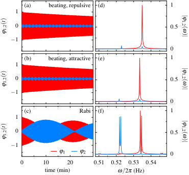
In Figs. 13(a) and 13(b) we present the deflections of both pendula for beating experiments without driving (, or ) for the two extreme coupling cases with the magnets aligned either antiparallel for maximal repulsion or collinear for maximal attraction, where the pivot distance mm corresponds to a small coupling. To initialize each measurement, we deflected just one of the two pendula, the one corresponding to the red lines. The energy transfer between the two pendula is clearly incomplete owing to the finite frequency detuning, mHz, while the beating frequency is . The latter corresponds to the difference between the respective eigenfrequencies, directly visible in the Fourier spectra shown in Figs. 13(d) and 13(e). The spectrum of the pendulum that was initially not deflected (blue) clearly contains two maxima, where the frequency of the smaller peak coincides with the main maximum of the initially deflected pendulum (red). This indicates a finite mixing between the states represented by and , which are not the exact eigenmodes because of the coupling between the pendula. Note, that the eigenfrequencies are slightly smaller for the attractive interaction as compared to the case of repulsive interaction.
In Fig. 13(c) we present the corresponding resonant Rabi experiment with identical parameters as above but the coupling being modulated with the angular frequency . In this case, the initial beating experiments mark the turning points of the modulation of the coupling during the Rabi experiment. The energy transfer between the two pendula is now complete but happens at the Rabi frequency , hence the initially postulated condition is fulfilled.
The Fourier spectra of the Rabi experiment in Fig. 13(f) reveal two main peaks and four side peaks for each pendulum. The main peaks are splitted by the (effective) Rabi frequency in Eq. (36). The much smaller side peaks, each of which is equally split by the (effective) Rabi frequency, are higher order components split off by multiples of from the main peaks. In the resonant case , the frequency values of the Fourier components of both pendula coincide, in the non-resonant case they would be displaced by . Note that the higher order components in the Fourier spectra are responsible for the weak stepwise modulation with frequency of the occupation of the pendula, which are weakly visible in Fig. 13(c).
F.2 LZSM experiments
For a direct comparison with the small coupling regime of Rabi experiments we perform similar measurements within the regime of LZSM experiments at much larger modulation of the coupling with . We consider measurements for mm, mHz, mHz and a sizable realized by including upper magnets. For such large couplings () the diabatic modes approximately correspond to the eigenmodes. Hence, in Fig. 14 we now plot . The beating experiments, which we again performed for collinear versus antiparallel magnets, summarized in the upper four panels of Fig. 14 reveal the expected much larger range of couplings compared to the Rabi experiment. The very different beating frequencies for attractive versus repulsive interactions point to a sizable . Note, that the frequency (main component of Fourier spectrum) of is almost identical for repulsive versus attractive coupling (blue in Figs. 14d and 14e), while the frequency of (red) varies by roughly 20 %.
The LZSM experiment, presented by its first avoided crossing in Fig. 14(c), shows the expected energy transfer between the in-phase and out-of-phase modes near the avoided crossing. The additional faster beats vary in frequency related with the time dependence of . The Fourier spectrum plotted in Fig. 14(f) comprises five modulation periods. It reveals that the in-phase mode stays at the frequency of the beating experiments, while the out-of-phase mode contains frequency components spanning a slightly larger region than that between the out-of-phase mode frequencies of the beating experiments. Note, that the apparent splitting, say , of the in-phase mode in the Fourier spectrum of the LZSM experiment resembles a slight difference between the frequencies that the in-phase mode has between attractive versus repulsive beating experiments. As a result, the the out-of phase mode spectrum is composed of two copies of a frequency comb with the same relative shift , each one characterized by equally spaced peaks separate by the modulation frequency .
F.3 Avoided crossings for Rabi versus LZSM experiments
Figure 15 summarizes the main components of the Fourier spectra of the experiments presented in Figs. 13 and 14 and thereby visualizes the vastly different experimental regimes realized in a Rabi experiment, where , versus a LZSM experiment with .
To highlight the differences between the regimes of the Rabi versus LZSM experiments, in Figs. 15(a) and 15(b) we plot for the Rabi versus LZSM experiments shown in Figs. 13 and 14 the relevant regions of the avoided crossings predicted for the measured frequencies by the Schrödinger equation (for the time independent quantum mechanical two-level system). The blue squares indicate the components of the respective Fourier spectra of the beating experiments, where we determined the values of using the eigenvalue equation . The red circles in Fig. 15(a) indicate the four main components of the Fourier spectra of the Rabi experiment in Fig. 13(f), where we used for simplicity. The line of red circles in Fig. 15(b) indicates the range of the frequency comb of the Fourier spectrum of of the LZSM experiment, cf. Fig. 14(f), where we again used for simplicity.
Appendix G Notations, units and magnitudes
| variable, definition | explanation | values |
|---|---|---|
| deflection angles of individual pendula | rad | |
| overall mass of each pendulum | 4.242 kg | |
| acceleration due to gravity in Munich (PTB table) | 9.807232 m/s2 | |
| resonance angular frequency of pendulum 1 | ||
| resonance angular frequency of pendulum 2 | ||
| reduced length of pendulum 1 | (0.818 - 0.912) m | |
| reduced length of pendulum 2 | 0.912 m | |
| center of mass of pendulum 1 (distance from pivot) | m | |
| center of mass of pendulum 2 (distance from pivot) | 0.841 m | |
| moment of inertia of pendulum 1 (respective pivot) | (2.619 - 3.254) kg m2 | |
| moment of inertia of pendulum 2 (respective pivot) | 3.254 kg m2 | |
| quality factor of individual uncoupled pendula | ||
| The following distances are equal for both pendula: | ||
| distance between pivot and point of measurement | 1.053 m | |
| distance between pivot and center of lower magnet | 1.148 m | |
| vertical distance between pivot and center of upper magnet | 0.635 m | |
| variable, definition | explanation | values and units |
|---|---|---|
| in-phase — out-of-phase mode | ||
| distance between pivots, i.e., lower magnets for | m | |
| magnetic moment of each lower magnet | 25.37 Am2 | |
| distance between upper magnets for | m | |
| magnetic moment of each upper magnet | 6.544 Am2 | |
| mean moment of inertia | kg m2 | |
| mean angular frequency of both pendula | s-1 | |
| angular frequency difference | ||
| coupling constant | () s-1 | |
| effective potential curvature (see Sec. A.3) | ||
| interaction energy between lower magnets | () J | |
| interaction energy between upper magnets | () J | |
| quality factor of coupled pendula (for realized range of ) |
| variable, definition | explanation | values and units |
|---|---|---|
| period of magnets’ rotation | 85.5 s, 141 s, 441 s | |
| modulated coupling constant (linear approximation) | s-1 | |
| rabi frequency for and if only lower magnets are used | ||
| Single passage Landau-Zener probability | ||
| Speed of driving at avoided crossing at | () s-2 | |
| Initial probability to occupy in-phase mode |
References
- Shore et al. (2009) B. W. Shore, M. V. Gromovyy, L. P. Yatsenko, and V. I. Romanenko, Simple mechanical analogs of rapid adiabatic passage in atomic physics, Am. J. Phys. 77, 1183 (2009).
- Rabi (1937) I. I. Rabi, Space quantization in a gyrating magnetic field, Phys. Rev. 51, 652 (1937).
- Landau (1932) L. D. Landau, Zur Theorie der Energieübertragung bei Stößen, Phys. Z. Sowjetunion 2, 46 (1932).
- Zener (1932) C. Zener, Non-adiabatic crossing of energy levels, Proc. R. Soc. London A 137, 696 (1932).
- Stueckelberg (1932) E. C. G. Stueckelberg, Theorie der unelastischen Stösse zwischen Atomen, Helv. Phys. Acta 5, 369 (1932).
- Majorana (1932) E. Majorana, Atomi orientati in campo magnetico variable, Nuovo Cimento 9, 43 (1932).
- Grønbech-Jensen and Cirillo (2005) N. Grønbech-Jensen and M. Cirillo, Rabi-type oscillations in a classical Josephson junction, Phys. Rev. Lett. 95, 067001 (2005).
- Novotny (2010) L. Novotny, Strong coupling, energy splitting, and level crossings: A classical perspective, Am. J. Phys. 78, 1199–1202 (2010).
- Heinrich et al. (2010) G. Heinrich, J. G. E. Harris, and F. Marquardt, Photon shuttle: Landau-Zener-Stückelberg dynamics in an optomechanical system, Phys. Rev. A 81, 011801(R) (2010).
- Frimmer and Novotny (2014) M. Frimmer and L. Novotny, The classical Bloch equations, Am. J. Phys. 82, 947–954 (2014).
- Ivakhnenko et al. (2018) O. V. Ivakhnenko, S. N. Shevchenko, and F. Nori, Simulating quantum dynamical phenomena using classical oscillators: Landau-Zener-Stückelberg-Majorana interferometry, latching modulation, and motional averaging, Sci. Rep. , 12218 (2018).
- Parafilo and Kiselev (2018) A. V. Parafilo and M. N. Kiselev, Tunable RKKY interaction in a double quantum dot nanoelectromechanical device, Phys. Rev. B 97, 035418 (2018).
- Süsstrunk and Huber (2015) R. Süsstrunk and S. D. Huber, Observation of phononic helical edge states in a mechanical topological insulator, Science 349, 47–50 (2015).
- Nash et al. (2015) L. M. Nash, D. Kleckner, A. Read, V. Vitelli, A. M. Turner, and W. T. M. Irvine, Topological mechanics of gyroscopic metamaterials, Proc. Nat. Acad. Sci. 112, 14495–14500 (2015).
- Faust et al. (2013) T. Faust, J. Rieger, M. J. Seitner, J. P. Kotthaus, and E. M. Weig, Coherent control of a classical nanomechanical two-level system, Nature Phys. 9, 485 (2013).
- Seitner et al. (2016) M. J. Seitner, H. Ribeiro, J. Kölbl, T. Faust, J. P. Kotthaus, and E. M. Weig, Classical Stückelberg interferometry of a nanomechanical two-mode system at room temperature, Phys. Rev. B 94, 245406 (2016).
- Mullen et al. (1989) K. Mullen, E. Ben-Jacob, Y. Gefen, and Z. Schuss, Time of Zener tunneling, Phys. Rev. Lett. 62, 2543 (1989).
- Vitanov (1999) N. V. Vitanov, Transition times in the Landau-Zener model, Phys. Rev. A 59, 988 (1999).
- Wubs et al. (2005) M. Wubs, K. Saito, S. Kohler, Y. Kayanuma, and P. Hänggi, Landau-Zener transitions in qubits controlled by electromagnetic fields, New J. Phys. 7, 218 (2005).
- Sillanpää et al. (2005) M. A. Sillanpää, T. Lehtinen, A. Paila, Y. Makhlin, L. Roschier, and P. J. Hakonen, Direct observation of Josephson capacitance, Phys. Rev. Lett. 95, 206806 (2005).
- Berns et al. (2008) D. M. Berns, M. S. Rudner, S. O. Valenzuela, K. K. Berggren, W. D. Oliver, L. S. Levitov, and T. P. Orlando, Amplitude spectroscopy of a solid-state artificial atom, Nature (London) 455, 51 (2008).
- Stehlik et al. (2012) J. Stehlik, Y. Dovzhenko, J. R. Petta, J. R. Johansson, F. Nori, H. Lu, and A. C. Gossard, Landau-Zener-Stückelberg interferometry of a single electron charge qubit, Phys. Rev. B 86, 121303(R) (2012).
- Forster et al. (2014) F. Forster, G. Petersen, S. Manus, P. Hänggi, D. Schuh, W. Wegscheider, S. Kohler, and S. Ludwig, Characterization of qubit dephasing by Landau-Zener-Stückelberg-Majorana interferometry, Phys. Rev. Lett. 112, 116803 (2014).
- Forster et al. (2015) F. Forster, M. Mühlbacher, R. Blattmann, D. Schuh, W. Wegscheider, S. Ludwig, and S. Kohler, Landau-Zener interference at bichromatic driving, Phys. Rev. B 92, 245422 (2015).
- Heinrich et al. (2021) A. J. Heinrich, W. D. Oliver, L. M. K. Vandersypen, A. Ardavan, R. Sessoli, D. Loss, A. Bleszynski Jayich, J. Fernandez-Rossier, A. Laucht, and A. Morello, Quantum-coherent nanoscience, Nature Nanotech. 16, 1318 (2021).
- (26) In the interaction term, we have neglected the small difference of the moments of interia. Moreover, the sign of is chosen such that it matches the usual definition in the quantum mechanical two-level problem. It is positive for attractive interaction.
- Shevchenko et al. (2010) S. N. Shevchenko, S. Ashhab, and F. Nori, Landau-Zener-Stückelberg interferometry, Phys. Rep. 492, 1 (2010).
- Ivakhnenko et al. (2023) O. V. Ivakhnenko, S. N. Shevchenko, and F. Nori, Nonadiabatic Landau-Zener-Stückelberg-Majorana transitions, dynamics, and interference, Phys. Rep. 995, 1 (2023).
- Mathieu (1868) E. Mathieu, Memoire sur le mouvement vibratoire d’une membrane de forme elliptique, J. Math. Pures Appl. 13, 137 (1868).
- Saito et al. (2006) K. Saito, M. Wubs, S. Kohler, P. Hänggi, and Y. Kayanuma, Quantum state preparation in circuit QED via Landau-Zener tunneling, Europhys. Lett. 76, 22 (2006).
- Ribeiro and Burkard (2009) H. Ribeiro and G. Burkard, Nuclear state preparation via Landau-Zener-Stückelberg transitions in double quantum dots, Phys. Rev. Lett. 102, 216802 (2009).
- Schrödinger (1926) E. Schrödinger, An undulatory theory of the mechanics of atoms and molecules, Phys. Rev. 28, 1049 (1926).
- Berry (1984) M. V. Berry, Quantal phase factors accompanying adiabatic changes, Proc. R. Soc. A 392, 45 (1984).
- Mi et al. (2018) X. Mi, S. Kohler, and J. R. Petta, Landau-Zener interferometry of valley-orbit states in Si/SiGe double quantum dots, Phys. Rev. B 98, 161404(R) (2018).
- Shevchenko et al. (2018) S. N. Shevchenko, A. I. Ryzhov, and F. Nori, Low-frequency spectroscopy for quantum multilevel systems, Phys. Rev. B 98, 195434 (2018).
- Menchon-Enrich et al. (2016) R. Menchon-Enrich, A. Benseny, V. Ahufinger, A. D. Greentree, T. Busch, and J. Mompart, Spatial adiabatic passage: a review of recent progress, Rep. Prog. Phys. 79, 074401 (2016).
- Leggett (2001) A. J. Leggett, Bose-Einstein condensation in the alkali gases: Some fundamental concepts, Rev. Mod. Phys. 73, 307 (2001).
- Goldstein et al. (2001) H. Goldstein, C. Poole Jr., and J. Safko, Classical Mechanics, 3rd ed. (Pearson, San Francisco, 2001).
- Jackson (1999) J. D. Jackson, Classical Electrodynamics, 3rd ed. (Wiley, New York, 1999).
- Cohen-Tannoudji et al. (1992) C. Cohen-Tannoudji, J. Dupont-Roc, and G. Grynberg, Atom photon interaction: Basic processes and applications (Wiley, New York, 1992).
- Oliver et al. (2005) W. D. Oliver, Y. Yu, J. C. Lee, K. K. Berggren, L. S. Levitov, and T. P. Orlando, Mach-zehnder interferometry in a strongly driven superconducting qubit, Science 310, 1653 (2005).
- Sillanpää et al. (2006) M. Sillanpää, T. Lehtinen, A. Paila, Y. Makhlin, and P. Hakonen, Continuous-time monitoring of Landau-Zener interference in a Cooper-pair box, Phys. Rev. Lett. 96, 187002 (2006).
- Wilson et al. (2007) C. M. Wilson, T. Duty, F. Persson, M. Sandberg, G. Johansson, and P. Delsing, Coherence times of dressed states of a superconducting qubit under extreme driving, Phys. Rev. Lett. 98, 257003 (2007).
- Izmalkov et al. (2008) A. Izmalkov, S. H. W. van der Ploeg, S. N. Shevchenko, M. Grajcar, E. Il’ichev, U. Hübner, A. N. Omelyanchouk, and H.-G. Meyer, Consistency of ground state and spectroscopic measurements on flux qubits, Phys. Rev. Lett. 101, 017003 (2008).
- Li et al. (2013) J. Li, M. P. Silveri, K. S. Kumar, J.-M. Pirkkalainen, A. Vepsäläinen, W. C. Chien, J. Tuorila, M. A. Sillanpää, P. J. Hakonen, E. V. Thuneberg, and G. S. Paraoanu, Motional averaging in a superconducting qubit, Nature Comm. 4, 1420 (2013).
- Dupont-Ferrier et al. (2013) E. Dupont-Ferrier, B. Roche, B. Voisin, X. Jehl, R. Wacquez, M. Vinet, M. Sanquer, and S. De Franceschi, Coherent coupling of two dopants in a silicon nanowire probed by Landau-Zener-Stückelberg interferometry, Phys. Rev. Lett. 110, 136802 (2013).
- Koski et al. (2018) J. V. Koski, A. J. Landig, A. Pályi, P. Scarlino, C. Reichl, W. Wegscheider, G. Burkard, A. Wallraff, K. Ensslin, and T. Ihn, Floquet spectroscopy of a strongly driven quantum dot charge qubit with a microwave resonator, Phys. Rev. Lett. 121, 043603 (2018).
- Chen et al. (2021) M.-B. Chen, B.-C. Wang, S. Kohler, Y. Kang, T. Lin, S.-S. Gu, H.-O. Li, G.-C. Guo, X. Hu, H.-W. Jiang, G. Cao, and G.-P. Guo, Floquet state depletion in ac-driven circuit QED, Phys. Rev. B 103, 205428 (2021).