Quantum Image Representation Methods Using Qutrits
Abstract
Quantum Image Processing is a recent highlight in the quantum computing field. All previous methods for representing the images as quantum states were defined using qubits. One Quantum Image Representation (QIR) method using qutrits is present in the literature. Inspired by the qubit methods and the higher state-space available for qutrits, multiple QIR methods using qutrits are worked out in this paper. The ternary quantum gates required for the representations are described, and then the implementation details for five qutrit-based QIR methods are given. All the methods have been simulated in software, and example circuits are provided.
Index Terms:
Qutrits, Quantum image representation, Quantum computationI Introduction
Quantum Image Processing research is in a nascent stage. Several qubit QIR methods are available in the literature. A review summarising many of them is also available [1]. In particular, FRQI [2], FRQCI [3], MCQI [4] and QRCI [5] methods are considered to provide their qutrit extensions in this paper. To the best of our knowledge, these extensions are novel. An approach to extend the NEQR [6] method was previously followed to define the QTRQ [7] method.
It has been well known for a long time that it is, in principle, possible to use qudits with more than two states to carry out Quantum Information Processing [8]. Compared to qubit, qudit systems provide a more extensive state-space to store and process information and can provide certain advantages such as reduction of the circuit depth/complexity [9, 10, 11]. In the present work, we are restricting our focus to qutrit-based computing. It is useful to note that there have been physical implementations of qutrit systems [12, 13]; Rigetti11 1 https://medium.com/rigetti/beyond-qubits-unlocking-the-third-state-in-quantum-processors-12d2f84133c4 has also announced experimental access to qutrits. While Cirq [14] already provides qudit simulation functionality, it is also under development at PennyLane [15].
II Qutrit Gates
The qutrit gates used in the implementations are described in this section.
II-A Single Qutrit Ternary Gates
A corresponding qutrit gate can be defined for any qubit gate by defining such that the action of is on basis states only [16]. This allows us to define three gates for qutrits:
| (1) | ||||
| (2) | ||||
| (3) |
By combining the action of these gates, two more single qutrit gates can be constructed:
II-A1 Single-Shift Gate
The action of this gate on a basis state is given by:
| (4) |
The gate is defined as:
| (5) |
II-A2 Double-Shift Gate
The action of this gate on a basis state is given by:
| (6) |
The gate is defined as:
| (7) |
This construction can be used to define Hadamard gates too. But, these versions do not create an equal superposition state.
II-A3 Ternary Hadamard Gate
The qutrit extension of the qubit Hadamard gate as defined in [7] is considered in this paper.
| (8) |
The action of the Hadamard gate on the basis states is given by:
| (9) | ||||
| (10) | ||||
| (11) |
This version of the qutrit Hadamard gate can thus be used on the state to get to an equal superposition of the three basis states without any phase.
II-A4 Ternary Rotation Gates
The definition of elementary one-qutrit gates as given in [16] is considered.
| (12) | ||||
| (13) | ||||
| (14) | ||||
| (15) |
Note that these rotation gates can also be obtained by using the previous construction.
The construction can also be used to get extensions of general single-qubit rotation gate . For example:
| (16) |
II-A5 Ternary Identity Gate
The identity gate for qutrits is the 3D identity matrix,
| (17) |
Its action on a state is given as:
| (18) |
II-B Controlled Qutrit Gates
Control qutrits for ternary gates can be in any of the three basis states. Thus, for each single-qutrit gate, three different controlled variations of two-qutrit gates (the control qutrit can be in any of or state), nine different three qutrit gates (the control qutrits can be in any of or state) and so on are possible. The decomposition of any such gate can be assured using the universality of qudit logic [10].
III Qutrit Quantum Image Representation Methods
Some QIR methods using qutrits are described in this section. Cirq has been used to simulate these methods. Cirq provides basic functionality to use qudits by allowing the use of custom quantum gates that can be defined for any dimension qudit. The gates used in the paper are not natively available and were defined with the definitions given in the previous section before use, another small contribution to the area through this work. The images considered for encoding are of dimension .


| R | G | B | ||||||||
| Y | 0 | 37 | 235 | 140 | 192 | 144 | 129 | 178 | 20 | 254 |
| 1 | 72 | 255 | 137 | 204 | 71 | 237 | 101 | 146 | 212 | |
| 2 | 203 | 133 | 79 | 252 | 134 | 25 | 139 | 252 | 234 | |
| 0 | 1 | 2 | 0 | 1 | 2 | 0 | 1 | 2 | ||
| X | ||||||||||
III-A FQRI
Inspired by the qubit FRQI method, the flexible qutrit representation of quantum images (FQRI) is proposed. The image information is encoded in a quantum state given by the formula:
| (19) |
qutrits are required to encode a image with qutrits used to encode the location information, and the remaining qutrit is used to encode the pixel values. The pixel values are encoded in the values where . For an 8-bit grayscale image, the pixel values are in the range , which are then scaled to be in ’s range.
The state can be prepared in two steps. First, the qutrit Hadamard gate is applied on the qutrits to create a superposition state. Then gates controlled on the location qutrits are applied. Formally:
- 1.
Begin with state.
- 2.
Apply transform :
(20) - 3.
Apply controlled gates for each pixel state :
(21) (22)
The circuit diagram pertinent to FQRI representation of the image in Fig. 1(a) is provided in Fig. Quantum Image Representation Methods Using Qutrits.
The decoding of the encoded image is probabilistic and depends on the number of shots used. The final state can be measured in the computational basis to get the probabilities of all different basis states. The values can be calculated from the probabilities.
This encoding works well for grayscale images. As only two of the three possible states of the pixel value qutrit are being used, this encoding can be hypothesised to be implemented with a qubit-qutrit hybrid model where qutrits are used for encoding the pixel location and a qubit is used for pixel values.
As mentioned earlier, all three states of the pixel value qutrit can be utilised to encode RGB information of colour images. This method is described in the following encoding.


III-B FQRRI
The flexible qutrit representation of RGB quantum images (FQRRI) is proposed here. In this encoding, qutrits are used to encode RGB images. Again assuming 8-bit images, all R, G and B pixel values will be in the range . The image is encoded in the quantum state given by:
| (23) |
Here, and encode the pixel values of G, B and G, R channels, respectively, of the pixel. The three values are encoded in two angles using the equations:
| (24) | |||
| (25) |
The symbol represents the floor division operation. Because of the particular structure of these equations, all three pixel values for all pixels can be obtained.
The decoding is probabilistic and depends on the number of shots used. The state is measured in the computational basis to get counts of all basis states. Each measurement will provide us with a ternary string. From this string, the last values give us the pixel location, and from the first value, the probability of getting and states can be calculated. Let’s call these probabilities and for the pixel, then,
| (26) | ||||
| (27) |
This gives,
| (28) | ||||
| (29) |
| (30) |
To create the state in (23), the steps to be followed are:
- 1.
Begin with state.
- 2.
Apply transform :
(31) - 3.
Apply controlled gates and controlled gates for each pixel state :
(32) (33) (34)
The circuit diagram for FQRRI of the image in Fig. 1(b) is shown in Fig. Quantum Image Representation Methods Using Qutrits.


III-C FQRQCI
The qubit FRQCI method uses the phase to encode an extra value in the quantum state. This still leaves two angles to encode three values. This, like FQRRI, needs more shots to decode the image accurately. The extra state available in qutrits can be used to encode the three pixel values in three different angles. This inspires the flexible qutrit representation of quantum color images (FQRQCI).
As before, qutrits are required to encode an RGB image. The quantum state of the image using this encoding is given by the formula:
| (35) |
where,
| (36) | |||
| (37) | |||
| (38) |
To create the state in (35), the steps to be followed are:
- 1.
Begin with state.
- 2.
Apply transform :
(39) - 3.
Apply controlled gates and controlled gates for each pixel state :
(40) (41) (42)


The circuit diagram for FQRQCI of the image in Fig. 1(b) is shown in Fig. Quantum Image Representation Methods Using Qutrits.
The decoding is probabilistic. To get back the pixel values, the following steps need to be performed:
- 1.
Measure the final state in the computational basis to get probabilities of and state of the pixel value qutrit, while the other qutrits provide information about the pixel location. Now,
(43) (44) - 2.
Apply the operation on the pixel value qutrit and again measure the final state in the computational basis to get .
- 3.
Separately, apply the operation on the pixel value qutrit and again measure the final state in the computational basis to get .
- 4.
Get the value as:
(45)
III-D MCQRI
The qubit MCQI method uses qubits to encode colour images with qubits used to encode pixel location, two qubits used to specify which colour to encode and the last qubit to encode the pixel value. The extra third state in qutrits can be used to specify which colour to use in a single qutrit. Thus, only qutrits can be used to encode RGB images. Inspired by this, the multi channel qutrit representation for quantum images (MCQRI) is proposed.
The quantum state of the image is given by the formula:
| (46) |
The pixel values are encoded in the values where by scaling. The following steps are followed to get to this state:
- 1.
Begin with state.
- 2.
Apply transform :
(47) - 3.
Apply three controlled gates for each pixel state :
(48) (49) (50) (51) (52) (53) The gates are controlled gates that are applied on the first two qutrits, which are in turn controlled by the last qutrits.


The circuit diagram for MCQRI of the image in Fig. 1(b) is shown in Fig. Quantum Image Representation Methods Using Qutrits.
The decoding is probabilistic and depends on the number of shots used. The original image can be obtained by measuring the state in the computational basis. Let denote the array of probabilities obtained after measuring the state. Assuming that the array is ordered in ascending order of the states, the size of the array will be . It can be divided into three equal parts. The first values correspond to values and the next values correspond to values. Let these be denoted by and respectively. The last values will be zero. Now,
| (54) |
These values are the values from (46). Again, this array can be divided into three equal parts. The first part corresponds to R values, next to G values and the last to B values which can then be scaled back to the range to obtain the original image.
One can also think of implementing this as a qubit-qutrit hybrid model with qutrits and one qubit.
III-E QRCIQ
All the previous encodings had probabilistic decoding. The encoding considered here provides a deterministic decoding process. The QTRQ method is the qutrit extension of the qubit NEQR method. The quantum representation model of color digital images using qutrits (QRCIQ), the qutrit extension of the qubit QRCI method, is proposed.
The encoding requires qutrits to encode RGB images. Here, qutrits are required to encode pixel location, the next two qutrits are used to encode the bit plane number, and the remaining three qutrits encode the bit plane value. Assuming 8-bit images, the quantum state is given by the formula:
| (55) |
Here, represents the bit plane number and is the RGB bit value of the pixel of plane. The bit plane values are . The state is prepared using the following steps:
- 1.
Begin with state.
- 2.
Apply transform :
(56) - 3.
If , where , do nothing.
- 4.
If , apply gate on the qutrit controlled by qutrits with control state .
- 5.
If , apply gate on the qutrit controlled by qutrits with control state .
The circuit diagram for QRCIQ of the image in Fig. 1(b) is shown in Fig. Quantum Image Representation Methods Using Qutrits.
The decoding is deterministic as after measuring the state in the computational basis, the mere presence of a basis state provides all information it encodes. The bit string of the basis state can be decoded to give the pixel location, bit plane number and the bit plane pixel value. It is important to note here that extra states will be present in the final state corresponding to unused bit planes. As two qutrits can encode bit planes and only six are required for an 8-bit image using ternary strings, three bit planes are empty, corresponding to or . Thus, while decoding, these states need to be discarded. It’s possible to envision that these available ”slots” can be populated to provide extra information about the images or facilitate processing or error correction.


Remark
The encodings that have a probabilistic decoding, use inverse trigonometric functions to calculate the encoded pixel values. These functions have a finite domain, for example, . The values calculated using a finite number of shots may fall outside the domain of these functions. Thus, the values need to be clipped to stay in the domain to get a valid result. The accuracy of the calculated values can be improved by increasing the number of shots. While QRCIQ does not have a probabilistic decoding and does not depend on the number of shots used, it still requires a minimum number of shots to observe all basis states at least once. Once all states have been observed, increasing the number of shots will have no effect on the decoding.
IV Conclusion and Future Work
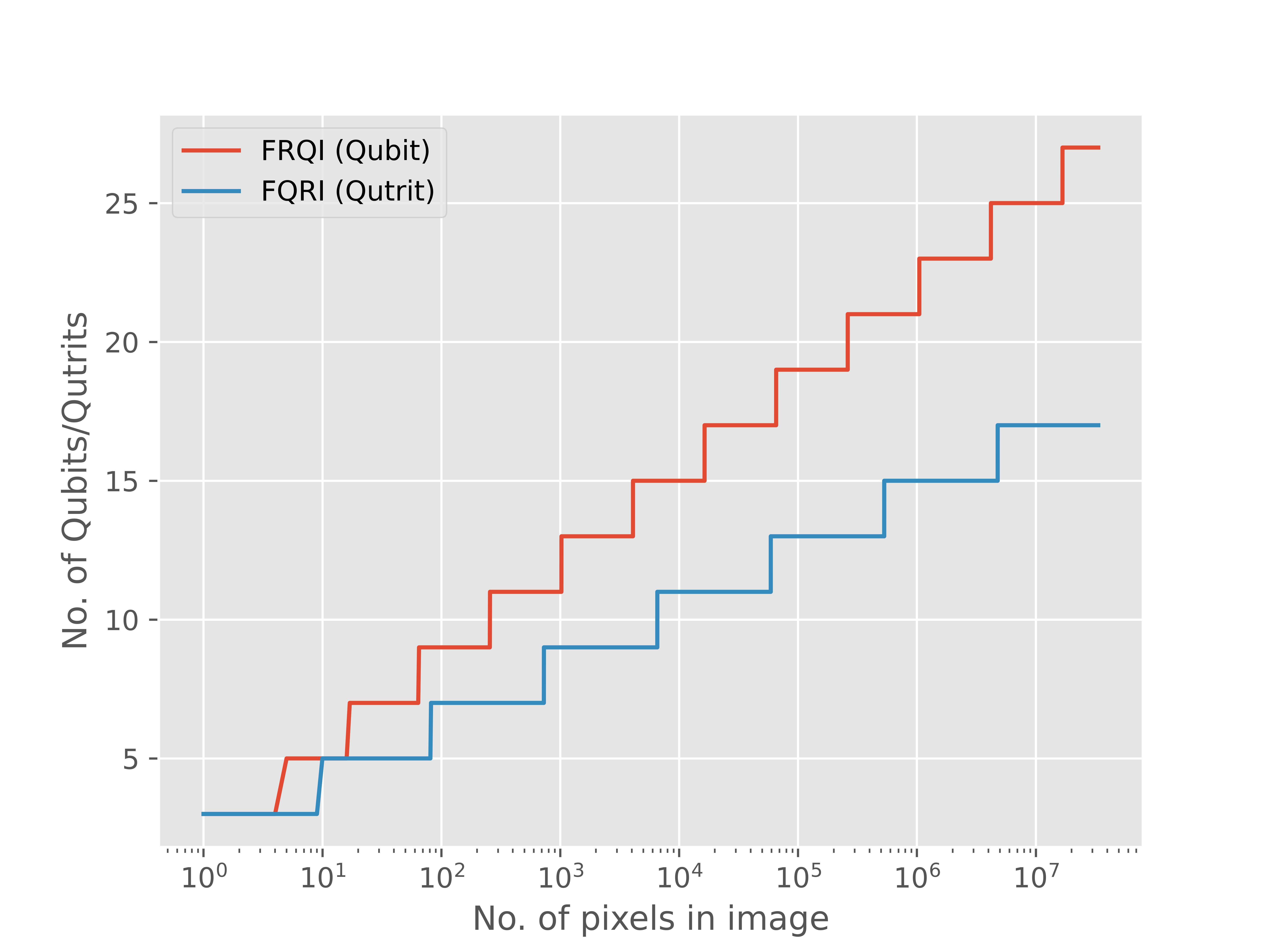
A few implementations to represent images as quantum states using qutrits have been described. All of these were validated using simulations with Cirq. While the decoding is probabilistic for most of them and depends on the number of shots used, it is also important to note that decoding the image is not the only use case for these representations. Different image processing tasks can be performed on the final quantum state [17, 18, 19, 20]. Machine learning tasks like classification can also be performed on the qutrit quantum representation of the images as performed with qubit QIRs [21, 22]. A summary of the provided methods is shown in Table II. The resource requirement increases slower than the qubit case and is always lower except for trivial cases. This can be seen from Fig. 7.
| QIR |
|
|
|
Equation | ||||||
|---|---|---|---|---|---|---|---|---|---|---|
| FQRI | Grayscale | Probabilistic | Eq. 19 | |||||||
| FQRRI | RGB | Probabilistic | Eq. 23 | |||||||
| FQRQCI | RGB | Probabilistic | Eq. 35 | |||||||
| MCQRI | RGB | Probabilistic | Eq. 46 | |||||||
| QRCIQ | RGB | Deterministic | Eq. 55 |
While from the universality of qudit logic, the decomposition of the multi-qutrit gates used can be assured, the decompositions have not been looked at in this paper. Research can be done to find optimal decompositions of the gates. More representations can be studied to utilise the extra state available in qutrits. Appropriate use of the empty slots can also be studied. Comparison of different representations on their effectiveness in various image processing tasks can also be explored.
References
- [1] J. Su, X. Guo, C. Liu, and L. Li, “A new trend of quantum image representations,” IEEE Access, vol. 8, pp. 214 520–214 537, 2020.
- [2] P. Q. Le, F. Dong, and K. Hirota, “A flexible representation of quantum images for polynomial preparation, image compression, and processing operations,” Quantum Information Processing, vol. 10, no. 1, pp. 63–84, Feb. 2011. [Online]. Available: https://doi.org/10.1007/s11128-010-0177-y
- [3] P. Li and X. Liu, “Color image representation model and its application based on an improved frqi,” International Journal of Quantum Information, vol. 16, no. 01, p. 1850005, 2018. [Online]. Available: https://doi.org/10.1142/S0219749918500053
- [4] B. Sun, A. M. Iliyasu, F. Yan, F. Dong, and K. Hirota, “An rgb multi-channel representation for images on quantum computers,” J. Adv. Comput. Intell. Intell. Informatics, vol. 17, pp. 404–417, 2013.
- [5] L. Wang, Q. Ran, J. Ma, S. Yu, and L. Tan, “Qrci: A new quantum representation model of color digital images,” Optics Communications, vol. 438, pp. 147–158, 2019. [Online]. Available: https://www.sciencedirect.com/science/article/pii/S003040181930015X
- [6] Y. Zhang, K. Lu, Y. Gao, and M. Wang, “Neqr: a novel enhanced quantum representation of digital images,” Quantum Information Processing, vol. 12, no. 8, pp. 2833–2860, Aug. 2013. [Online]. Available: https://doi.org/10.1007/s11128-013-0567-z
- [7] H. Dong, D. Lu, and C. Li, “A novel qutrit representation of quantum image,” Quantum Information Processing, vol. 21, no. 3, p. 108, Mar. 2022. [Online]. Available: https://doi.org/10.1007/s11128-022-03450-8
- [8] M. Kues, C. Reimer, P. Roztocki, L. R. Cortés, S. Sciara, B. Wetzel, Y. Zhang, A. Cino, S. T. Chu, B. E. Little, D. J. Moss, L. Caspani, J. Azaña, and R. Morandotti, “On-chip generation of high-dimensional entangled quantum states and their coherent control,” Nature, vol. 546, no. 7660, pp. 622–626, Jun. 2017. [Online]. Available: https://doi.org/10.1038/nature22986
- [9] B. P. Lanyon, M. Barbieri, M. P. Almeida, T. Jennewein, T. C. Ralph, K. J. Resch, G. J. Pryde, J. L. O’Brien, A. Gilchrist, and A. G. White, “Simplifying quantum logic using higher-dimensional hilbert spaces,” Nature Physics, vol. 5, no. 2, pp. 134–140, Feb. 2009. [Online]. Available: https://doi.org/10.1038/nphys1150
- [10] Y. Wang, Z. Hu, B. C. Sanders, and S. Kais, “Qudits and high-dimensional quantum computing,” Frontiers in Physics, vol. 8, 2020. [Online]. Available: https://www.frontiersin.org/articles/10.3389/fphy.2020.589504
- [11] T. C. Ralph, K. J. Resch, and A. Gilchrist, “Efficient toffoli gates using qudits,” Phys. Rev. A, vol. 75, p. 022313, Feb. 2007. [Online]. Available: https://link.aps.org/doi/10.1103/PhysRevA.75.022313
- [12] M. A. Yurtalan, J. Shi, M. Kononenko, A. Lupascu, and S. Ashhab, “Implementation of a walsh-hadamard gate in a superconducting qutrit,” Phys. Rev. Lett., vol. 125, p. 180504, Oct. 2020. [Online]. Available: https://link.aps.org/doi/10.1103/PhysRevLett.125.180504
- [13] M. S. Blok, V. V. Ramasesh, T. Schuster, K. O’Brien, J. M. Kreikebaum, D. Dahlen, A. Morvan, B. Yoshida, N. Y. Yao, and I. Siddiqi, “Quantum information scrambling on a superconducting qutrit processor,” Phys. Rev. X, vol. 11, p. 021010, Apr. 2021. [Online]. Available: https://link.aps.org/doi/10.1103/PhysRevX.11.021010
- [14] C. Developers, “Cirq,” Apr. 2022, See full list of authors on Github: https://github .com/quantumlib/Cirq/graphs/contributors. [Online]. Available: https://doi.org/10.5281/zenodo.6599601
- [15] V. Bergholm, J. Izaac, M. Schuld, C. Gogolin, M. S. Alam, S. Ahmed, J. M. Arrazola, C. Blank, A. Delgado, S. Jahangiri, K. McKiernan, J. J. Meyer, Z. Niu, A. Száva, and N. Killoran, “Pennylane: Automatic differentiation of hybrid quantum-classical computations,” 2018. [Online]. Available: https://arxiv.org/abs/1811.04968
- [16] Y.-M. Di and H.-R. Wei, “Elementary gates for ternary quantum logic circuit,” 2011. [Online]. Available: https://arxiv.org/abs/1105.5485
- [17] A. Anand, M. Lyu, P. S. Baweja, and V. Patil, “Quantum image processing,” 2022. [Online]. Available: https://arxiv.org/abs/2203.01831
- [18] Y. Ruan, X. Xue, and Y. Shen, “Quantum image processing: Opportunities and challenges,” Mathematical Problems in Engineering, vol. 2021, p. 6671613, Jan. 2021. [Online]. Available: https://doi.org/10.1155/2021/6671613
- [19] F. Yan and S. E. Venegas-Andraca, Quantum Image Processing. Springer Singapore, 2020. [Online]. Available: http://dx.doi.org/10.1007/978-981-32-9331-1
- [20] S. Caraiman and V. Manta, “Image processing using quantum computing,” in 2012 16th International Conference on System Theory, Control and Computing (ICSTCC), 2012, pp. 1–6.
- [21] A. Khandelwal, M. G. Chandra, and S. Pramanik, “On classifying images using quantum image representation,” 2022. [Online]. Available: https://arxiv.org/abs/2206.11509
- [22] A. Mohsen and M. Tiwari, “Image compression and classification using qubits and quantum deep learning,” 2021. [Online]. Available: https://arxiv.org/abs/2110.05476
@*=¡0em¿@R=1em @C=0.75em
*!R!¡.5em,0em¿=¡0em¿ @- [0,-1] @- [0,-1]*+¡.6em¿R_y^(01)(0.14) @- [0,-1]@- [0,-1]*+¡.6em¿R_y^(02)(2.39) @- [0,-1]@- [0,-1]*+¡.6em¿R_y^(01)(0.02) @- [0,-1]@- [0,-1]*+¡.6em¿R_y^(02)(1.95) @- [0,-1]@- [0,-1]*+¡.6em¿R_y^(01)(0.39) @- [0,-1]@- [0,-1]*+¡.6em¿R_y^(02)(1.68) @- [0,-1]@- [0,-1]*+¡.6em¿R_y^(01)(2.43) @- [0,-1]@- [0,-1]*+¡.6em¿R_y^(02)(2.41) @- [0,-1]@- [0,-1]*+¡.6em¿R_y^(01)(1.49) @- [0,-1]@- [0,-1]*+¡.6em¿R_y^(02)(0.98) @- [0,-1]@- [0,-1]*+¡.6em¿R_y^(01)(2.72) @- [0,-1]@- [0,-1]*+¡.6em¿R_y^(02)(2.85) @- [0,-1]@- [0,-1]*+¡.6em¿R_y^(01)(2.46) @- [0,-1]@- [0,-1]*+¡.6em¿R_y^(02)(3.1) @- [0,-1]@- [0,-1]*+¡.6em¿R_y^(01)(1.37) @- [0,-1]@- [0,-1]*+¡.6em¿R_y^(02)(1.67) @- [0,-1]@- [0,-1]*+¡.6em¿R_y^(01)(1.95) @- [0,-1]@- [0,-1]*+¡.6em¿R_y^(02)(0.26) @- [0,-1]@- [0,-1]@¡- [0,-1]
*!R!¡.5em,0em¿=¡0em¿ @- [0,-1]*+¡.6em¿H @- [0,-1]@- [0,-1]* @- [0,-1]@- [-1,0]* @- [0,-1]@- [-1,0]* @- [0,-1]@- [-1,0]* @- [0,-1]@- [-1,0]* @- [0,-1]@- [-1,0]* @- [0,-1]@- [-1,0]* @- [0,-1]@- [-1,0]* @- [0,-1]@- [-1,0]* @- [0,-1]@- [-1,0]* @- [0,-1]@- [-1,0]* @- [0,-1]@- [-1,0]* @- [0,-1]@- [-1,0]* @- [0,-1]@- [-1,0]* @- [0,-1]@- [-1,0]* @- [0,-1]@- [-1,0]* @- [0,-1]@- [-1,0]* @- [0,-1]@- [-1,0]* @- [0,-1]@- [-1,0] @¡- [0,-1]
*!R!¡.5em,0em¿=¡0em¿ @- [0,-1]*+¡.6em¿H @- [0,-1]@- [0,-1]* @- [0,-1]@- [-1,0]* @- [0,-1]@- [-1,0]* @- [0,-1]@- [-1,0]* @- [0,-1]@- [-1,0]* @- [0,-1]@- [-1,0]* @- [0,-1]@- [-1,0]* @- [0,-1]@- [-1,0]* @- [0,-1]@- [-1,0]* @- [0,-1]@- [-1,0]* @- [0,-1]@- [-1,0]* @- [0,-1]@- [-1,0]* @- [0,-1]@- [-1,0]* @- [0,-1]@- [-1,0]* @- [0,-1]@- [-1,0]* @- [0,-1]@- [-1,0]* @- [0,-1]@- [-1,0]* @- [0,-1]@- [-1,0]* @- [0,-1]@- [-1,0] @¡- [0,-1]
@*=¡0em¿@R=1em @C=0.75em
*!R!¡.5em,0em¿=¡0em¿ @- [0,-1] @- [0,-1]*+¡.6em¿R_y^(01)(0.46) @- [0,-1]@- [0,-1]*+¡.6em¿U^(12)(2.37, 2.19, 0) @- [0,-1]@- [0,-1]*+¡.6em¿R_y^(01)(2.9) @- [0,-1]@- [0,-1]*+¡.6em¿U^(12)(1.77, 0.25, 0) @- [0,-1]@- [0,-1]*+¡.6em¿R_y^(01)(1.72) @- [0,-1]@- [0,-1]*+¡.6em¿U^(12)(1.59, 3.13, 0) @- [0,-1]@- [0,-1]*+¡.6em¿R_y^(01)(0.89) @- [0,-1]@- [0,-1]*+¡.6em¿U^(12)(2.51, 1.24, 0) @- [0,-1]@- [0,-1]*+¡.6em¿R_y^(01)(3.14) @- [0,-1]@- [0,-1]*+¡.6em¿U^(12)(0.87, 1.8, 0) @- [0,-1]@- [0,-1]*+¡.6em¿R_y^(01)(1.69) @- [0,-1]@- [0,-1]*+¡.6em¿U^(12)(2.92, 2.61, 0) @- [0,-1]@- [0,-1]*+¡.6em¿R_y^(01)(2.5) @- [0,-1]@- [0,-1]*+¡.6em¿U^(12)(3.1, 1.71, 0) @- [0,-1]@- [0,-1]*+¡.6em¿R_y^(01)(1.64) @- [0,-1]@- [0,-1]*+¡.6em¿U^(12)(1.65, 3.1, 0) @- [0,-1]@- [0,-1]*+¡.6em¿R_y^(01)(0.97) @- [0,-1]@- [0,-1]*+¡.6em¿U^(12)(0.31, 2.88, 0) @- [0,-1]@- [0,-1]@¡- [0,-1]
*!R!¡.5em,0em¿=¡0em¿ @- [0,-1]*+¡.6em¿H @- [0,-1]@- [0,-1]* @- [0,-1]@- [-1,0]* @- [0,-1]@- [-1,0]* @- [0,-1]@- [-1,0]* @- [0,-1]@- [-1,0]* @- [0,-1]@- [-1,0]* @- [0,-1]@- [-1,0]* @- [0,-1]@- [-1,0]* @- [0,-1]@- [-1,0]* @- [0,-1]@- [-1,0]* @- [0,-1]@- [-1,0]* @- [0,-1]@- [-1,0]* @- [0,-1]@- [-1,0]* @- [0,-1]@- [-1,0]* @- [0,-1]@- [-1,0]* @- [0,-1]@- [-1,0]* @- [0,-1]@- [-1,0]* @- [0,-1]@- [-1,0]* @- [0,-1]@- [-1,0] @¡- [0,-1]
*!R!¡.5em,0em¿=¡0em¿ @- [0,-1]*+¡.6em¿H @- [0,-1]@- [0,-1]* @- [0,-1]@- [-1,0]* @- [0,-1]@- [-1,0]* @- [0,-1]@- [-1,0]* @- [0,-1]@- [-1,0]* @- [0,-1]@- [-1,0]* @- [0,-1]@- [-1,0]* @- [0,-1]@- [-1,0]* @- [0,-1]@- [-1,0]* @- [0,-1]@- [-1,0]* @- [0,-1]@- [-1,0]* @- [0,-1]@- [-1,0]* @- [0,-1]@- [-1,0]* @- [0,-1]@- [-1,0]* @- [0,-1]@- [-1,0]* @- [0,-1]@- [-1,0]* @- [0,-1]@- [-1,0]* @- [0,-1]@- [-1,0]* @- [0,-1]@- [-1,0] @¡- [0,-1]
@*=¡0em¿@R=1em @C=0.75em
*!R!¡.5em,0em¿=¡0em¿ @- [0,-1] @- [0,-1]*+¡.6em¿R_y^(01)(0.46) @- [0,-1]@- [0,-1]*+¡.6em¿R_y^(01)(0.89) @- [0,-1]@- [0,-1]*+¡.6em¿R_y^(01)(2.5) @- [0,-1]@- [0,-1]*+¡.6em¿R_y^(01)(2.9) @- [0,-1]@- [0,-1]*+¡.6em¿R_y^(01)(3.14) @- [0,-1]@- [0,-1]*+¡.6em¿R_y^(01)(1.64) @- [0,-1]@- [0,-1]*+¡.6em¿R_y^(01)(1.72) @- [0,-1]@- [0,-1]*+¡.6em¿R_y^(01)(1.69) @- [0,-1]@- [0,-1]*+¡.6em¿R_y^(01)(0.97) @- [0,-1]@- [0,-1]*+¡.6em¿R_y^(01)(2.37) @- [0,-1]@- [0,-1]*+¡.6em¿R_y^(01)(2.51) @- [0,-1]@- [0,-1]*+¡.6em¿R_y^(01)(3.1) @- [0,-1]@- [0,-1]*+¡.6em¿R_y^(01)(1.77) @- [0,-1]@- [0,-1]*+¡.6em¿R_y^(01)(0.87) @- [0,-1]@- [0,-1]*+¡.6em¿R_y^(01)(1.65) @- [0,-1]@- [0,-1]*+¡.6em¿R_y^(01)(1.59) @- [0,-1]@- [0,-1]*+¡.6em¿R_y^(01)(2.92) @- [0,-1]@- [0,-1]*+¡.6em¿R_y^(01)(0.31) @- [0,-1]@- [0,-1]*+¡.6em¿R_y^(01)(2.19) @- [0,-1]@- [0,-1]*+¡.6em¿R_y^(01)(1.24) @- [0,-1]@- [0,-1]*+¡.6em¿R_y^(01)(1.71) @- [0,-1]@- [0,-1]*+¡.6em¿R_y^(01)(0.25) @- [0,-1]@- [0,-1]*+¡.6em¿R_y^(01)(1.8) @- [0,-1]@- [0,-1]*+¡.6em¿R_y^(01)(3.1) @- [0,-1]@- [0,-1]*+¡.6em¿R_y^(01)(3.13) @- [0,-1]@- [0,-1]*+¡.6em¿R_y^(01)(2.61) @- [0,-1]@- [0,-1]*+¡.6em¿R_y^(01)(2.88) @- [0,-1]@- [0,-1]@¡- [0,-1]
*!R!¡.5em,0em¿=¡0em¿ @- [0,-1]*+¡.6em¿H @- [0,-1]@- [0,-1]* @- [0,-1]@- [-1,0]* @- [0,-1]@- [-1,0]* @- [0,-1]@- [-1,0]* @- [0,-1]@- [-1,0]* @- [0,-1]@- [-1,0]* @- [0,-1]@- [-1,0]* @- [0,-1]@- [-1,0]* @- [0,-1]@- [-1,0]* @- [0,-1]@- [-1,0]* @- [0,-1]@- [-1,0]* @- [0,-1]@- [-1,0]* @- [0,-1]@- [-1,0]* @- [0,-1]@- [-1,0]* @- [0,-1]@- [-1,0]* @- [0,-1]@- [-1,0]* @- [0,-1]@- [-1,0]* @- [0,-1]@- [-1,0]* @- [0,-1]@- [-1,0]* @- [0,-1]@- [-1,0]* @- [0,-1]@- [-1,0]* @- [0,-1]@- [-1,0]* @- [0,-1]@- [-1,0]* @- [0,-1]@- [-1,0]* @- [0,-1]@- [-1,0]* @- [0,-1]@- [-1,0]* @- [0,-1]@- [-1,0]* @- [0,-1]@- [-1,0] @¡- [0,-1]
*!R!¡.5em,0em¿=¡0em¿ @- [0,-1]*+¡.6em¿H @- [0,-1]@- [0,-1]* @- [0,-1]@- [-1,0]* @- [0,-1]@- [-1,0]* @- [0,-1]@- [-1,0]* @- [0,-1]@- [-1,0]* @- [0,-1]@- [-1,0]* @- [0,-1]@- [-1,0]* @- [0,-1]@- [-1,0]* @- [0,-1]@- [-1,0]* @- [0,-1]@- [-1,0]* @- [0,-1]@- [-1,0]* @- [0,-1]@- [-1,0]* @- [0,-1]@- [-1,0]* @- [0,-1]@- [-1,0]* @- [0,-1]@- [-1,0]* @- [0,-1]@- [-1,0]* @- [0,-1]@- [-1,0]* @- [0,-1]@- [-1,0]* @- [0,-1]@- [-1,0]* @- [0,-1]@- [-1,0]* @- [0,-1]@- [-1,0]* @- [0,-1]@- [-1,0]* @- [0,-1]@- [-1,0]* @- [0,-1]@- [-1,0]* @- [0,-1]@- [-1,0]* @- [0,-1]@- [-1,0]* @- [0,-1]@- [-1,0]* @- [0,-1]@- [-1,0] @¡- [0,-1]
*!R!¡.5em,0em¿=¡0em¿ @- [0,-1]*+¡.6em¿H @- [0,-1]@- [0,-1]* @- [0,-1]@- [-1,0]* @- [0,-1]@- [-1,0]* @- [0,-1]@- [-1,0]* @- [0,-1]@- [-1,0]* @- [0,-1]@- [-1,0]* @- [0,-1]@- [-1,0]* @- [0,-1]@- [-1,0]* @- [0,-1]@- [-1,0]* @- [0,-1]@- [-1,0]* @- [0,-1]@- [-1,0]* @- [0,-1]@- [-1,0]* @- [0,-1]@- [-1,0]* @- [0,-1]@- [-1,0]* @- [0,-1]@- [-1,0]* @- [0,-1]@- [-1,0]* @- [0,-1]@- [-1,0]* @- [0,-1]@- [-1,0]* @- [0,-1]@- [-1,0]* @- [0,-1]@- [-1,0]* @- [0,-1]@- [-1,0]* @- [0,-1]@- [-1,0]* @- [0,-1]@- [-1,0]* @- [0,-1]@- [-1,0]* @- [0,-1]@- [-1,0]* @- [0,-1]@- [-1,0]* @- [0,-1]@- [-1,0]* @- [0,-1]@- [-1,0] @¡- [0,-1]
@*=¡0em¿@R=1em @C=0.75em
*!R!¡.5em,0em¿=¡0em¿ @- [0,-1] @- [0,-1] @- [0,-1]*+¡.6em¿+1 @- [0,-1]@- [0,-1] @- [0,-1] @- [0,-1] @- [0,-1] @- [0,-1] @- [0,-1]*+¡.6em¿+2 @- [0,-1]@- [0,-1] @- [0,-1]*+¡.6em¿+2 @- [0,-1]@- [0,-1] @- [0,-1] @- [0,-1]*+¡.6em¿+2 @- [0,-1]@- [0,-1] @- [0,-1] @- [0,-1]*+¡.6em¿+2 @- [0,-1]@- [0,-1]*+¡.6em¿+1 @- [0,-1]@- [0,-1] @- [0,-1] @- [0,-1]*+¡.6em¿+1 @- [0,-1]@- [0,-1] @- [0,-1]*+¡.6em¿+1 @- [0,-1]@- [0,-1] @- [0,-1] @- [0,-1]*+¡.6em¿+2 @- [0,-1]@- [0,-1] @- [0,-1]*+¡.6em¿+1 @- [0,-1]@- [0,-1] @- [0,-1] @- [0,-1]*+¡.6em¿+1 @- [0,-1]@- [0,-1] @- [0,-1] @- [0,-1]*+¡.6em¿+1 @- [0,-1]@- [0,-1] @- [0,-1] @- [0,-1] @- [0,-1] @- [0,-1] @- [0,-1]*+¡.6em¿+2 @- [0,-1]@- [0,-1] @- [0,-1]*+¡.6em¿+1 @- [0,-1]@- [0,-1] @- [0,-1]*+¡.6em¿+2 @- [0,-1]@- [0,-1] @- [0,-1]*!L!¡-.5em,0em¿=¡0em¿⋯ @- [0,-1]
*!R!¡.5em,0em¿=¡0em¿ @- [0,-1] @- [0,-1]*+¡.6em¿+1 @- [0,-1]@- [0,-1] @- [0,-1]@- [-1,0] @- [0,-1]*+¡.6em¿+1 @- [0,-1]@- [0,-1]*+¡.6em¿+2 @- [0,-1]@- [0,-1] @- [0,-1] @- [0,-1] @- [0,-1]@- [-1,0]*+¡.6em¿+1 @- [0,-1]@- [0,-1] @- [0,-1]@- [-1,0]*+¡.6em¿+1 @- [0,-1]@- [0,-1] @- [0,-1] @- [0,-1]@- [-1,0] @- [0,-1]*+¡.6em¿+1 @- [0,-1]@- [0,-1] @- [0,-1]@- [-1,0] @- [0,-1]@- [-1,0]*+¡.6em¿+1 @- [0,-1]@- [0,-1] @- [0,-1] @- [0,-1]@- [-1,0] @- [0,-1] @- [0,-1]@- [-1,0]*+¡.6em¿+2 @- [0,-1]@- [0,-1] @- [0,-1] @- [0,-1]@- [-1,0] @- [0,-1] @- [0,-1]@- [-1,0]*+¡.6em¿+1 @- [0,-1]@- [0,-1] @- [0,-1] @- [0,-1]@- [-1,0]*+¡.6em¿+2 @- [0,-1]@- [0,-1] @- [0,-1] @- [0,-1]@- [-1,0]*+¡.6em¿+2 @- [0,-1]@- [0,-1] @- [0,-1]*+¡.6em¿+1 @- [0,-1]@- [0,-1]*+¡.6em¿+2 @- [0,-1]@- [0,-1] @- [0,-1] @- [0,-1]@- [-1,0] @- [0,-1] @- [0,-1]@- [-1,0]*+¡.6em¿+2 @- [0,-1]@- [0,-1] @- [0,-1]@- [-1,0]*+¡.6em¿+1 @- [0,-1]@- [0,-1]*!L!¡-.5em,0em¿=¡0em¿⋯ @- [0,-1]
*!R!¡.5em,0em¿=¡0em¿ @- [0,-1] @- [0,-1] @- [0,-1]@- [-1,0] @- [0,-1]@- [-1,0]*+¡.6em¿+1 @- [0,-1]@- [0,-1] @- [0,-1]@- [-1,0] @- [0,-1]@- [-1,0]*+¡.6em¿+1 @- [0,-1]@- [0,-1]*+¡.6em¿+1 @- [0,-1]@- [0,-1] @- [0,-1]@- [-1,0] @- [0,-1]@- [-1,0] @- [0,-1]@- [-1,0] @- [0,-1]@- [-1,0]*+¡.6em¿+1 @- [0,-1]@- [0,-1] @- [0,-1]@- [-1,0]*+¡.6em¿+2 @- [0,-1]@- [0,-1] @- [0,-1]@- [-1,0] @- [0,-1]@- [-1,0] @- [0,-1]@- [-1,0] @- [0,-1]@- [-1,0]*+¡.6em¿+2 @- [0,-1]@- [0,-1] @- [0,-1]@- [-1,0]*+¡.6em¿+2 @- [0,-1]@- [0,-1] @- [0,-1]@- [-1,0] @- [0,-1]@- [-1,0]*+¡.6em¿+2 @- [0,-1]@- [0,-1] @- [0,-1]@- [-1,0]*+¡.6em¿+2 @- [0,-1]@- [0,-1] @- [0,-1]@- [-1,0] @- [0,-1]@- [-1,0]*+¡.6em¿+2 @- [0,-1]@- [0,-1] @- [0,-1]@- [-1,0] @- [0,-1]@- [-1,0]*+¡.6em¿+1 @- [0,-1]@- [0,-1] @- [0,-1]@- [-1,0] @- [0,-1]@- [-1,0]*+¡.6em¿+2 @- [0,-1]@- [0,-1] @- [0,-1]@- [-1,0] @- [0,-1]@- [-1,0]*+¡.6em¿+1 @- [0,-1]@- [0,-1] @- [0,-1]@- [-1,0]*+¡.6em¿+2 @- [0,-1]@- [0,-1] @- [0,-1]@- [-1,0] @- [0,-1]@- [-1,0] @- [0,-1]@- [-1,0] @- [0,-1]@- [-1,0]*!L!¡-.5em,0em¿=¡0em¿⋯ @- [0,-1]
*!R!¡.5em,0em¿=¡0em¿ @- [0,-1]*+¡.6em¿H @- [0,-1]@- [0,-1] * @- [0,-1]@- [-1,0] * @- [0,-1]@- [-1,0] * @- [0,-1]@- [-1,0] * @- [0,-1]@- [-1,0] * @- [0,-1]@- [-1,0] * @- [0,-1]@- [-1,0] * @- [0,-1]@- [-1,0] * @- [0,-1]@- [-1,0] * @- [0,-1]@- [-1,0] * @- [0,-1]@- [-1,0] * @- [0,-1]@- [-1,0] * @- [0,-1]@- [-1,0] * @- [0,-1]@- [-1,0] * @- [0,-1]@- [-1,0] * @- [0,-1]@- [-1,0] * @- [0,-1]@- [-1,0] * @- [0,-1]@- [-1,0] * @- [0,-1]@- [-1,0] * @- [0,-1]@- [-1,0] * @- [0,-1]@- [-1,0] * @- [0,-1]@- [-1,0] * @- [0,-1]@- [-1,0] * @- [0,-1]@- [-1,0] * @- [0,-1]@- [-1,0] * @- [0,-1]@- [-1,0] * @- [0,-1]@- [-1,0] * @- [0,-1]@- [-1,0] * @- [0,-1]@- [-1,0] * @- [0,-1]@- [-1,0] * @- [0,-1]@- [-1,0] * @- [0,-1]@- [-1,0] * @- [0,-1]@- [-1,0] * @- [0,-1]@- [-1,0] * @- [0,-1]@- [-1,0] * @- [0,-1]@- [-1,0] * @- [0,-1]@- [-1,0] * @- [0,-1]@- [-1,0] * @- [0,-1]@- [-1,0] * @- [0,-1]@- [-1,0] * @- [0,-1]@- [-1,0] * @- [0,-1]@- [-1,0] * @- [0,-1]@- [-1,0] * @- [0,-1]@- [-1,0] * @- [0,-1]@- [-1,0]*!L!¡-.5em,0em¿=¡0em¿⋯ @- [0,-1]
*!R!¡.5em,0em¿=¡0em¿ @- [0,-1]*+¡.6em¿H @- [0,-1]@- [0,-1] * @- [0,-1]@- [-1,0] * @- [0,-1]@- [-1,0] * @- [0,-1]@- [-1,0] * @- [0,-1]@- [-1,0] * @- [0,-1]@- [-1,0] * @- [0,-1]@- [-1,0] * @- [0,-1]@- [-1,0] * @- [0,-1]@- [-1,0] * @- [0,-1]@- [-1,0] * @- [0,-1]@- [-1,0] * @- [0,-1]@- [-1,0] * @- [0,-1]@- [-1,0] * @- [0,-1]@- [-1,0] * @- [0,-1]@- [-1,0] * @- [0,-1]@- [-1,0] * @- [0,-1]@- [-1,0] * @- [0,-1]@- [-1,0] * @- [0,-1]@- [-1,0] * @- [0,-1]@- [-1,0] * @- [0,-1]@- [-1,0] * @- [0,-1]@- [-1,0] * @- [0,-1]@- [-1,0] * @- [0,-1]@- [-1,0] * @- [0,-1]@- [-1,0] * @- [0,-1]@- [-1,0] * @- [0,-1]@- [-1,0] * @- [0,-1]@- [-1,0] * @- [0,-1]@- [-1,0] * @- [0,-1]@- [-1,0] * @- [0,-1]@- [-1,0] * @- [0,-1]@- [-1,0] * @- [0,-1]@- [-1,0] * @- [0,-1]@- [-1,0] * @- [0,-1]@- [-1,0] * @- [0,-1]@- [-1,0] * @- [0,-1]@- [-1,0] * @- [0,-1]@- [-1,0] * @- [0,-1]@- [-1,0] * @- [0,-1]@- [-1,0] * @- [0,-1]@- [-1,0] * @- [0,-1]@- [-1,0] * @- [0,-1]@- [-1,0] * @- [0,-1]@- [-1,0] * @- [0,-1]@- [-1,0]*!L!¡-.5em,0em¿=¡0em¿⋯ @- [0,-1]
*!R!¡.5em,0em¿=¡0em¿ @- [0,-1]*+¡.6em¿H @- [0,-1]@- [0,-1] * @- [0,-1]@- [-1,0] * @- [0,-1]@- [-1,0] * @- [0,-1]@- [-1,0] * @- [0,-1]@- [-1,0] * @- [0,-1]@- [-1,0] * @- [0,-1]@- [-1,0] * @- [0,-1]@- [-1,0] * @- [0,-1]@- [-1,0] * @- [0,-1]@- [-1,0] * @- [0,-1]@- [-1,0] * @- [0,-1]@- [-1,0] * @- [0,-1]@- [-1,0] * @- [0,-1]@- [-1,0] * @- [0,-1]@- [-1,0] * @- [0,-1]@- [-1,0] * @- [0,-1]@- [-1,0] * @- [0,-1]@- [-1,0] * @- [0,-1]@- [-1,0] * @- [0,-1]@- [-1,0] * @- [0,-1]@- [-1,0] * @- [0,-1]@- [-1,0] * @- [0,-1]@- [-1,0] * @- [0,-1]@- [-1,0] * @- [0,-1]@- [-1,0] * @- [0,-1]@- [-1,0] * @- [0,-1]@- [-1,0] * @- [0,-1]@- [-1,0] * @- [0,-1]@- [-1,0] * @- [0,-1]@- [-1,0] * @- [0,-1]@- [-1,0] * @- [0,-1]@- [-1,0] * @- [0,-1]@- [-1,0] * @- [0,-1]@- [-1,0] * @- [0,-1]@- [-1,0] * @- [0,-1]@- [-1,0] * @- [0,-1]@- [-1,0] * @- [0,-1]@- [-1,0] * @- [0,-1]@- [-1,0] * @- [0,-1]@- [-1,0] * @- [0,-1]@- [-1,0] * @- [0,-1]@- [-1,0] * @- [0,-1]@- [-1,0] * @- [0,-1]@- [-1,0] * @- [0,-1]@- [-1,0]*!L!¡-.5em,0em¿=¡0em¿⋯ @- [0,-1]
*!R!¡.5em,0em¿=¡0em¿ @- [0,-1]*+¡.6em¿H @- [0,-1]@- [0,-1] * @- [0,-1]@- [-1,0] * @- [0,-1]@- [-1,0] * @- [0,-1]@- [-1,0] * @- [0,-1]@- [-1,0] * @- [0,-1]@- [-1,0] * @- [0,-1]@- [-1,0] * @- [0,-1]@- [-1,0] * @- [0,-1]@- [-1,0] * @- [0,-1]@- [-1,0] * @- [0,-1]@- [-1,0] * @- [0,-1]@- [-1,0] * @- [0,-1]@- [-1,0] * @- [0,-1]@- [-1,0] * @- [0,-1]@- [-1,0] * @- [0,-1]@- [-1,0] * @- [0,-1]@- [-1,0] * @- [0,-1]@- [-1,0] * @- [0,-1]@- [-1,0] * @- [0,-1]@- [-1,0] * @- [0,-1]@- [-1,0] * @- [0,-1]@- [-1,0] * @- [0,-1]@- [-1,0] * @- [0,-1]@- [-1,0] * @- [0,-1]@- [-1,0] * @- [0,-1]@- [-1,0] * @- [0,-1]@- [-1,0] * @- [0,-1]@- [-1,0] * @- [0,-1]@- [-1,0] * @- [0,-1]@- [-1,0] * @- [0,-1]@- [-1,0] * @- [0,-1]@- [-1,0] * @- [0,-1]@- [-1,0] * @- [0,-1]@- [-1,0] * @- [0,-1]@- [-1,0] * @- [0,-1]@- [-1,0] * @- [0,-1]@- [-1,0] * @- [0,-1]@- [-1,0] * @- [0,-1]@- [-1,0] * @- [0,-1]@- [-1,0] * @- [0,-1]@- [-1,0] * @- [0,-1]@- [-1,0] * @- [0,-1]@- [-1,0] * @- [0,-1]@- [-1,0] * @- [0,-1]@- [-1,0]*!L!¡-.5em,0em¿=¡0em¿⋯ @- [0,-1]
@*=¡0em¿@R=1em @C=0.75em
*!R!¡.5em,0em¿=¡0em¿⋯*+¡.6em¿+1 @- [0,-1]@- [0,-1] @- [0,-1] @- [0,-1] @- [0,-1] @- [0,-1]*+¡.6em¿+1 @- [0,-1]@- [0,-1] @- [0,-1] @- [0,-1]*+¡.6em¿+1 @- [0,-1]@- [0,-1] @- [0,-1] @- [0,-1]*+¡.6em¿+1 @- [0,-1]@- [0,-1] @- [0,-1] @- [0,-1]*+¡.6em¿+2 @- [0,-1]@- [0,-1] @- [0,-1] @- [0,-1] @- [0,-1] @- [0,-1] @- [0,-1] @- [0,-1]*+¡.6em¿+1 @- [0,-1]@- [0,-1] @- [0,-1] @- [0,-1]*+¡.6em¿+1 @- [0,-1]@- [0,-1] @- [0,-1]*+¡.6em¿+2 @- [0,-1]@- [0,-1] @- [0,-1] @- [0,-1] @- [0,-1] @- [0,-1]*+¡.6em¿+2 @- [0,-1]@- [0,-1] @- [0,-1]*+¡.6em¿+1 @- [0,-1]@- [0,-1]*+¡.6em¿+1 @- [0,-1]@- [0,-1] @- [0,-1] @- [0,-1] @- [0,-1]*+¡.6em¿+2 @- [0,-1]@- [0,-1] @- [0,-1] @- [0,-1] @- [0,-1] @- [0,-1] @- [0,-1]*+¡.6em¿+1 @- [0,-1]@- [0,-1] @- [0,-1] @- [0,-1]*+¡.6em¿+2 @- [0,-1]@- [0,-1] @- [0,-1] @- [0,-1]*+¡.6em¿+1 @- [0,-1]@- [0,-1] @¡- [0,-1]
*!R!¡.5em,0em¿=¡0em¿⋯ @- [0,-1]@- [-1,0]*+¡.6em¿+2 @- [0,-1]@- [0,-1] @- [0,-1]*+¡.6em¿+1 @- [0,-1]@- [0,-1] @- [0,-1] @- [0,-1]@- [-1,0]*+¡.6em¿+1 @- [0,-1]@- [0,-1] @- [0,-1] @- [0,-1]@- [-1,0]*+¡.6em¿+2 @- [0,-1]@- [0,-1] @- [0,-1] @- [0,-1]@- [-1,0]*+¡.6em¿+2 @- [0,-1]@- [0,-1] @- [0,-1] @- [0,-1]@- [-1,0]*+¡.6em¿+1 @- [0,-1]@- [0,-1] @- [0,-1]*+¡.6em¿+1 @- [0,-1]@- [0,-1] @- [0,-1] @- [0,-1]*+¡.6em¿+1 @- [0,-1]@- [0,-1] @- [0,-1]@- [-1,0]*+¡.6em¿+2 @- [0,-1]@- [0,-1] @- [0,-1] @- [0,-1]@- [-1,0] @- [0,-1] @- [0,-1]@- [-1,0]*+¡.6em¿+2 @- [0,-1]@- [0,-1] @- [0,-1]*+¡.6em¿+2 @- [0,-1]@- [0,-1] @- [0,-1] @- [0,-1]@- [-1,0] @- [0,-1] @- [0,-1]@- [-1,0] @- [0,-1]@- [-1,0]*+¡.6em¿+1 @- [0,-1]@- [0,-1] @- [0,-1] @- [0,-1] @- [0,-1]@- [-1,0]*+¡.6em¿+1 @- [0,-1]@- [0,-1] @- [0,-1]*+¡.6em¿+2 @- [0,-1]@- [0,-1]*+¡.6em¿+2 @- [0,-1]@- [0,-1] @- [0,-1] @- [0,-1]@- [-1,0]*+¡.6em¿+2 @- [0,-1]@- [0,-1] @- [0,-1] @- [0,-1]@- [-1,0]*+¡.6em¿+2 @- [0,-1]@- [0,-1] @- [0,-1] @- [0,-1]@- [-1,0] @¡- [0,-1]
*!R!¡.5em,0em¿=¡0em¿⋯ @- [0,-1]@- [-1,0] @- [0,-1]@- [-1,0]*+¡.6em¿+2 @- [0,-1]@- [0,-1] @- [0,-1]@- [-1,0]*+¡.6em¿+2 @- [0,-1]@- [0,-1] @- [0,-1]@- [-1,0] @- [0,-1]@- [-1,0]*+¡.6em¿+2 @- [0,-1]@- [0,-1] @- [0,-1]@- [-1,0] @- [0,-1]@- [-1,0]*+¡.6em¿+2 @- [0,-1]@- [0,-1] @- [0,-1]@- [-1,0] @- [0,-1]@- [-1,0]*+¡.6em¿+1 @- [0,-1]@- [0,-1] @- [0,-1]@- [-1,0] @- [0,-1]@- [-1,0]*+¡.6em¿+2 @- [0,-1]@- [0,-1] @- [0,-1]@- [-1,0]*+¡.6em¿+2 @- [0,-1]@- [0,-1]*+¡.6em¿+1 @- [0,-1]@- [0,-1] @- [0,-1]@- [-1,0] @- [0,-1]@- [-1,0] @- [0,-1]@- [-1,0]*+¡.6em¿+2 @- [0,-1]@- [0,-1] @- [0,-1]@- [-1,0]*+¡.6em¿+1 @- [0,-1]@- [0,-1] @- [0,-1]@- [-1,0] @- [0,-1]@- [-1,0]*+¡.6em¿+1 @- [0,-1]@- [0,-1] @- [0,-1]@- [-1,0]*+¡.6em¿+2 @- [0,-1]@- [0,-1] @- [0,-1]@- [-1,0]*+¡.6em¿+1 @- [0,-1]@- [0,-1] @- [0,-1]@- [-1,0] @- [0,-1]@- [-1,0] @- [0,-1]@- [-1,0]*+¡.6em¿+2 @- [0,-1]@- [0,-1]*+¡.6em¿+2 @- [0,-1]@- [0,-1] @- [0,-1]@- [-1,0] @- [0,-1]@- [-1,0]*+¡.6em¿+1 @- [0,-1]@- [0,-1] @- [0,-1]@- [-1,0] @- [0,-1]@- [-1,0]*+¡.6em¿+1 @- [0,-1]@- [0,-1] @- [0,-1]@- [-1,0] @- [0,-1]@- [-1,0]*+¡.6em¿+2 @- [0,-1]@- [0,-1] @- [0,-1]@- [-1,0] @- [0,-1]@- [-1,0]*+¡.6em¿+2 @- [0,-1]@- [0,-1] @- [0,-1]@- [-1,0] @¡- [0,-1]
*!R!¡.5em,0em¿=¡0em¿⋯* @- [0,-1]@- [-1,0]* @- [0,-1]@- [-1,0]* @- [0,-1]@- [-1,0]* @- [0,-1]@- [-1,0]* @- [0,-1]@- [-1,0]* @- [0,-1]@- [-1,0]* @- [0,-1]@- [-1,0]* @- [0,-1]@- [-1,0]* @- [0,-1]@- [-1,0]* @- [0,-1]@- [-1,0]* @- [0,-1]@- [-1,0]* @- [0,-1]@- [-1,0]* @- [0,-1]@- [-1,0]* @- [0,-1]@- [-1,0]* @- [0,-1]@- [-1,0]* @- [0,-1]@- [-1,0]* @- [0,-1]@- [-1,0]* @- [0,-1]@- [-1,0]* @- [0,-1]@- [-1,0]* @- [0,-1]@- [-1,0]* @- [0,-1]@- [-1,0]* @- [0,-1]@- [-1,0]* @- [0,-1]@- [-1,0]* @- [0,-1]@- [-1,0]* @- [0,-1]@- [-1,0]* @- [0,-1]@- [-1,0]* @- [0,-1]@- [-1,0]* @- [0,-1]@- [-1,0]* @- [0,-1]@- [-1,0]* @- [0,-1]@- [-1,0]* @- [0,-1]@- [-1,0]* @- [0,-1]@- [-1,0]* @- [0,-1]@- [-1,0]* @- [0,-1]@- [-1,0]* @- [0,-1]@- [-1,0]* @- [0,-1]@- [-1,0]* @- [0,-1]@- [-1,0]* @- [0,-1]@- [-1,0]* @- [0,-1]@- [-1,0]* @- [0,-1]@- [-1,0]* @- [0,-1]@- [-1,0]* @- [0,-1]@- [-1,0]* @- [0,-1]@- [-1,0]* @- [0,-1]@- [-1,0]* @- [0,-1]@- [-1,0]* @- [0,-1]@- [-1,0]* @- [0,-1]@- [-1,0]* @- [0,-1]@- [-1,0]* @- [0,-1]@- [-1,0]* @- [0,-1]@- [-1,0]* @- [0,-1]@- [-1,0] @¡- [0,-1]
*!R!¡.5em,0em¿=¡0em¿⋯* @- [0,-1]@- [-1,0]* @- [0,-1]@- [-1,0]* @- [0,-1]@- [-1,0]* @- [0,-1]@- [-1,0]* @- [0,-1]@- [-1,0]* @- [0,-1]@- [-1,0]* @- [0,-1]@- [-1,0]* @- [0,-1]@- [-1,0]* @- [0,-1]@- [-1,0]* @- [0,-1]@- [-1,0]* @- [0,-1]@- [-1,0]* @- [0,-1]@- [-1,0]* @- [0,-1]@- [-1,0]* @- [0,-1]@- [-1,0]* @- [0,-1]@- [-1,0]* @- [0,-1]@- [-1,0]* @- [0,-1]@- [-1,0]* @- [0,-1]@- [-1,0]* @- [0,-1]@- [-1,0]* @- [0,-1]@- [-1,0]* @- [0,-1]@- [-1,0]* @- [0,-1]@- [-1,0]* @- [0,-1]@- [-1,0]* @- [0,-1]@- [-1,0]* @- [0,-1]@- [-1,0]* @- [0,-1]@- [-1,0]* @- [0,-1]@- [-1,0]* @- [0,-1]@- [-1,0]* @- [0,-1]@- [-1,0]* @- [0,-1]@- [-1,0]* @- [0,-1]@- [-1,0]* @- [0,-1]@- [-1,0]* @- [0,-1]@- [-1,0]* @- [0,-1]@- [-1,0]* @- [0,-1]@- [-1,0]* @- [0,-1]@- [-1,0]* @- [0,-1]@- [-1,0]* @- [0,-1]@- [-1,0]* @- [0,-1]@- [-1,0]* @- [0,-1]@- [-1,0]* @- [0,-1]@- [-1,0]* @- [0,-1]@- [-1,0]* @- [0,-1]@- [-1,0]* @- [0,-1]@- [-1,0]* @- [0,-1]@- [-1,0]* @- [0,-1]@- [-1,0]* @- [0,-1]@- [-1,0]* @- [0,-1]@- [-1,0]* @- [0,-1]@- [-1,0]* @- [0,-1]@- [-1,0]* @- [0,-1]@- [-1,0] @¡- [0,-1]
*!R!¡.5em,0em¿=¡0em¿⋯* @- [0,-1]@- [-1,0]* @- [0,-1]@- [-1,0]* @- [0,-1]@- [-1,0]* @- [0,-1]@- [-1,0]* @- [0,-1]@- [-1,0]* @- [0,-1]@- [-1,0]* @- [0,-1]@- [-1,0]* @- [0,-1]@- [-1,0]* @- [0,-1]@- [-1,0]* @- [0,-1]@- [-1,0]* @- [0,-1]@- [-1,0]* @- [0,-1]@- [-1,0]* @- [0,-1]@- [-1,0]* @- [0,-1]@- [-1,0]* @- [0,-1]@- [-1,0]* @- [0,-1]@- [-1,0]* @- [0,-1]@- [-1,0]* @- [0,-1]@- [-1,0]* @- [0,-1]@- [-1,0]* @- [0,-1]@- [-1,0]* @- [0,-1]@- [-1,0]* @- [0,-1]@- [-1,0]* @- [0,-1]@- [-1,0]* @- [0,-1]@- [-1,0]* @- [0,-1]@- [-1,0]* @- [0,-1]@- [-1,0]* @- [0,-1]@- [-1,0]* @- [0,-1]@- [-1,0]* @- [0,-1]@- [-1,0]* @- [0,-1]@- [-1,0]* @- [0,-1]@- [-1,0]* @- [0,-1]@- [-1,0]* @- [0,-1]@- [-1,0]* @- [0,-1]@- [-1,0]* @- [0,-1]@- [-1,0]* @- [0,-1]@- [-1,0]* @- [0,-1]@- [-1,0]* @- [0,-1]@- [-1,0]* @- [0,-1]@- [-1,0]* @- [0,-1]@- [-1,0]* @- [0,-1]@- [-1,0]* @- [0,-1]@- [-1,0]* @- [0,-1]@- [-1,0]* @- [0,-1]@- [-1,0]* @- [0,-1]@- [-1,0]* @- [0,-1]@- [-1,0]* @- [0,-1]@- [-1,0]* @- [0,-1]@- [-1,0]* @- [0,-1]@- [-1,0]* @- [0,-1]@- [-1,0]* @- [0,-1]@- [-1,0] @¡- [0,-1]
*!R!¡.5em,0em¿=¡0em¿⋯* @- [0,-1]@- [-1,0]* @- [0,-1]@- [-1,0]* @- [0,-1]@- [-1,0]* @- [0,-1]@- [-1,0]* @- [0,-1]@- [-1,0]* @- [0,-1]@- [-1,0]* @- [0,-1]@- [-1,0]* @- [0,-1]@- [-1,0]* @- [0,-1]@- [-1,0]* @- [0,-1]@- [-1,0]* @- [0,-1]@- [-1,0]* @- [0,-1]@- [-1,0]* @- [0,-1]@- [-1,0]* @- [0,-1]@- [-1,0]* @- [0,-1]@- [-1,0]* @- [0,-1]@- [-1,0]* @- [0,-1]@- [-1,0]* @- [0,-1]@- [-1,0]* @- [0,-1]@- [-1,0]* @- [0,-1]@- [-1,0]* @- [0,-1]@- [-1,0]* @- [0,-1]@- [-1,0]* @- [0,-1]@- [-1,0]* @- [0,-1]@- [-1,0]* @- [0,-1]@- [-1,0]* @- [0,-1]@- [-1,0]* @- [0,-1]@- [-1,0]* @- [0,-1]@- [-1,0]* @- [0,-1]@- [-1,0]* @- [0,-1]@- [-1,0]* @- [0,-1]@- [-1,0]* @- [0,-1]@- [-1,0]* @- [0,-1]@- [-1,0]* @- [0,-1]@- [-1,0]* @- [0,-1]@- [-1,0]* @- [0,-1]@- [-1,0]* @- [0,-1]@- [-1,0]* @- [0,-1]@- [-1,0]* @- [0,-1]@- [-1,0]* @- [0,-1]@- [-1,0]* @- [0,-1]@- [-1,0]* @- [0,-1]@- [-1,0]* @- [0,-1]@- [-1,0]* @- [0,-1]@- [-1,0]* @- [0,-1]@- [-1,0]* @- [0,-1]@- [-1,0]* @- [0,-1]@- [-1,0]* @- [0,-1]@- [-1,0]* @- [0,-1]@- [-1,0]* @- [0,-1]@- [-1,0]* @- [0,-1]@- [-1,0] @¡- [0,-1]