Long-lived Solitons and Their Signatures in the Classical Heisenberg ChainPreprint: APS/123-QED
Abstract
Motivated by the KPZ scaling recently observed in the classical ferromagnetic Heisenberg chain, we investigate the role of solitonic excitations in this model. We find that the Heisenberg chain, although well-known to be non-integrable, supports a two-parameter family of long-lived solitons. We connect these to the exact soliton solutions of the integrable Ishimori chain with interactions. We explicitly construct infinitely long-lived stationary solitons, and provide an adiabatic construction procedure for moving soliton solutions, which shows that Ishimori solitons have a long-lived Heisenberg counterpart when they are not too narrow and not too fast-moving. Finally, we demonstrate their presence in thermal states of the Heisenberg chain, even when the typical soliton width is larger than the spin correlation length, and argue that these excitations likely underlie the KPZ scaling.
Introduction— There has been renewed interest in understanding the long-time dynamics of classical many-body systems, in particular regarding the scope of anomalous, non-diffusive, transport. A paradigmatic phenomenon is Kardar-Parisi-Zhang (KPZ) scaling Kardar et al. 1986, associated with (generalised) hydrodynamics Bertini et al. 2016; Bulchandani et al. 2017; Doyon et al. 2018a; Doyon 2019; Castro-Alvaredo et al. 2016; Bulchandani et al. 2018; Schemmer et al. 2019; Das et al. 2020; Doyon et al. 2018b; Doyon et al. 2018a; Doyon 2019 and integrability Mendl and Spohn 2016; Mendl and Spohn 2014; Kulkarni et al. 2015; De Nardis et al. 2018; Chen et al. 2018; Das et al. 2019; Das et al. 2020; Roy et al. 2022; McRoberts et al. 2022; Lepri et al. 2020; Spohn 2014; Das et al. 2014; Gamayun et al. 2019; Krajnik and Prosen 2020; Bulchandani 2020. Recent theoretical developments have identified integrability and non-abelian symmetry as key ingredients for KPZ physics Prosen and Žunkovič 2013; Krajnik and Prosen 2020; De Nardis et al. 2021; Ilievski et al. 2021; Dupont and Moore 2020; Das et al. 2019; Bulchandani 2020.
Indeed, KPZ scaling is now established Das et al. 2019; Das et al. 2020 in the integrable Ishimori chain Ishimori 1982, also known as the integrable lattice-Landau-Lifshitz model. Intriguingly, the simple non-integrable nearest-neighbour classical Heisenberg chain was also found to host a long-lived regime of KPZ scaling at low temperature McRoberts et al. 2022, and it was subsequently noted that KPZ scaling in the Ishimori chain persists under spin-symmetry preserving perturbations Roy et al. 2022.

Whilst the classical Heisenberg spin chain is a widely studied system and a paradigmatic model of magnetism, it remains far from completely understood. For example, predictions of its hydrodynamics have involved ordinary diffusion Gerling and Landau 1989; Gerling and Landau 1990; Böhm et al. 1993; Srivastava et al. 1994; Oganesyan et al. 2009; Bagchi 2013; Glorioso et al. 2021 or different forms of anomalous behaviour Müller 1988; de Alcantara Bonfim and Reiter 1992; de Alcantara Bonfim and Reiter 1993; De Nardis et al. 2020a. Our recent observation of KPZ behaviour up to enormously large scales McRoberts et al. 2022 thus raises the question: does the Heisenberg chain exhibit properties ordinarily associated with integrability? In particular, one might wonder if this phenomenology can be related to magnon dynamics or the existence of solitons, thought to be crucial for KPZ behaviour both in quantum Bulchandani 2020; De Nardis et al. 2020b; Gopalakrishnan and Vasseur 2019; De Nardis et al. 2021; Ljubotina et al. 2019 and classical integrable 1D spin systems Bulchandani 2020; Das et al. 2019; Das et al. 2020; Roy et al. 2022.
In this letter, we demonstrate the existence of long-lived solitons in the classical Heisenberg chain. The appellation soliton is justified by an explicit continuous connection to those of the Ishimori chain via an interpolating Hamiltonian. We provide a direct construction of stable (infinitely long-lived) stationary isolated solitons, as well as an adiabatic construction of moving solitons. A central result is the existence of a family of solitons which are stable over a broad parameter regime (see Fig. 1(a)). This is, a priori, very surprising for a chain so far believed to be essentially generic. Beyond the isolated solitons, we study two-soliton scattering and observe behaviour quite analogous to that of the integrable model. Finally, for low-temperature thermal states, we show that solitons are present and can be individually identified even when their density is high. Taken together, these observations provide a physical basis for the robust KPZ scaling observed at low temperatures in the Heisenberg chain.
Models— The classical Heisenberg Hamiltonian is
| (1) |
where are classical vectors at sites of a chain, with nearest-neighbour ferromagnetic interaction strength .
The integrable Ishimori 1982; Theodorakopoulos 1995; Theodorakopoulos 1988; Faddeev and Takhtajan 1987; Sklyanin 1988; Sklyanin 1982; Prosen and Žunkovič 2013 Ishimori Hamiltonian,
| (2) |
possesses an extensive set of locally conserved charges, besides energy and magnetisation, such as the torsion
| (3) |
We interpolate smoothly between the chains,
| (4) |
with the Ishimori chain corresponding to , and the Heisenberg chain to the limit , preserving symmetry throughout. We set in the following.
One-Soliton Solutions— In the Ishimori chain Ishimori 1982, these are indexed by two physical parameters: an inverse-width and a wavenumber , see SI sup for explicit expressions and their properties.
The Heisenberg chain (1), by contrast, is not integrable. We next provide exact (though not closed-form) expressions for stationary solitons in the form of an (implicit) solution to the non-linear equations of motion of the Heisenberg model.
For this, we use canonical co-ordinates, , . Our ansatz is based on the structure of the stationary () Ishimori solitons. We assume (i) stationarity of the z-components, i.e., , (ii) spatially uniform azimuthal angles (except for a discontinuity of across the centre), and (iii) a uniform rotation frequency of the in-plane spin-components, i.e., . This ansatz reduces the equations of motion to a set of consistency equations for the ,
| (7) |
which, for a chosen frequency , may be solved numerically to arbitrary precision sup.
This yields stable stationary solitons of arbitrary width (), implying that the existence diagram in Fig. 1(a) extends to infinity on the x-axis. An example of a soliton obtained from the solution of these equations is shown in Fig. 1(b). This constitutes the first (to our knowledge) exact soliton in the Heisenberg model.
Adiabatic connection— We next connect these stationary solitons to those in the Ishimori chain by continuously tuning the interpolating Hamiltonian (4) between the two via a -smooth interpolation,
| (8) |
from at to at some long adiabatic time . We evolve an initial Ishimori soliton under the dynamics of Eq. (4), with this time-dependent given by Eq. (8), for some adiabatic time ; we then evolve up to some later time under the Heisenberg dynamics (1).
This continuously transforms stationary solitons of the Ishimori chain into stationary solitons of the Heisenberg chain with the same magnetisation.
Moving solitons— As the connection between the stationary solitons of the two models does not guarantee the existence of moving soliton solutions of the Heisenberg chain, we next use our adiabatic procedure to extend the ‘existence diagram’ in Fig 1(a) to finite . We consider a resultant state a soliton of the Heisenberg chain if the following conditions are satisfied: (i) there is, for all times, a unique local minimum of ; (ii) for , the torsion is constant in time; (iii) the unique local minimum propagates with a constant velocity. These conditions are examined in more detail in sup. An example of a thus constructed moving soliton is shown in Fig. 1(c), and compared to the original Ishimori soliton.
The resulting existence diagram (Fig. 1(a)), shows that the solitons are stable in the Heisenberg model over a remarkably large range of parameters , with the narrow solitons apparently becoming unstable first with increasing velocity ().
We find no indication of a finite lifetime of the single soliton states which are stable under this adiabatic procedure. Moreover, the torsion – generally not a conserved quantity of the Heisenberg chain – is conserved in these states. Whilst stationary solutions of non-linear classical equations of motion are well known (see e.g. Flach and Gorbach 2008), stable moving solitons are not generally expected to exist.
Next we consider how the properties of Ishimori solitons are modified in the Heisenberg model. Fig. 2 shows that the internal frequency (the frequency with which the in-plane spin-components rotate) and velocity of a Heisenberg soliton are suppressed. The energy (measured in both cases by the Heisenberg Hamiltonian) is only slightly reduced – whilst the torsion is very slightly higher for the Heisenberg solitons (see also Fig. S2, sup). Overall, we note a remarkable similarity between the one-soliton properties in the Ishimori and Heisenberg chain.
Two-soliton scattering— We now turn to interactions between the solitons. To set the stage, we briefly recall scattering in the Ishimori chain. As a fully integrable model, interactions are completely described by the two-soliton phase-shifts, even for thermal multi-soliton states Theodorakopoulos 1995; Theodorakopoulos 1988. When two solitons collide, the asymptotic result (compared to two separate one-soliton solutions) is unchanged, except that the solitons are displaced by a so-called phase-shift Theodorakopoulos 1995:
| (9) |
experienced by the soliton , due to a collision with the soliton .
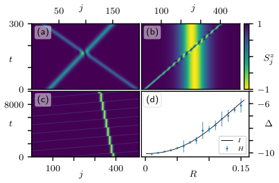
Fig. 3 displays the scattering of two Heisenberg solitons. The solitons survive scattering essentially unchanged (Fig. 3(a)), akin to the fully integrable model. Whilst the collisions do leave the solitons unchanged asymptotically, the magnetisation of a moving soliton is ‘screened’ during the collision with a larger soliton as seen in Fig. 3(b). Importantly, solitons survive multiple collisions (Fig. 3(c)), with the change to their trajectories apparently given by simple consecutive phase-shifts.
There exist, nonetheless, some important differences between the Heisenberg and Ishimori cases. First, absent integrability, scattering in the Heisenberg chain is not expected to be perfectly lossless. Indeed, there is a very small amount of radiation emitted during the collision (approx. in magnitude) in Fig. 3(a). Second, scattering from narrow solitons at small (where the existence diagram is wider in ) can emit significant amounts of radiation, although, curiously, the modified solitons that emerge appear to be stable to subsequent collisions.
In addition, the phase-shift appears not to depend only on the soliton parameters . We extract the phase-shifts in Fig. 3(d) by averaging over 10 scattering events. They are also averaged over the relative phase (azimuthal angles) of the solitons at the moment of collision. In the integrable case, this has no effect – in the Heisenberg case, however, in particular for larger , the phase-shift depends on the relative phase (see Fig. S5). We discuss these points in more detail in sup.
Despite these differences, however, we emphasise that collisions over a large parameter regime in the Heisenberg model strongly resemble the scattering in the Ishimori case. Importantly, whilst the phase-shift acquires some fluctuations, the velocities of the solitons remain unaffected by the collisions.
Solitons in thermal states— Whilst the Heisenberg chain supports solitons as stable solitary waves, which suffer only very weak dissipation in scattering events, the imperfect nature of the scattering implies the existence of a thermal timescale on which they eventually decay. The question arises, then, as to what extent these solitons exert their influence on the hydrodynamics and transport properties: thermal states are not in any sense a dilute soliton gas, and it would not be unreasonable to expect solitons to experience so many scattering events that, unprotected by integrability, they collapse too swiftly to generate a discernible superdiffusive contribution to the transport of spin or energy.
We find that the torsion (3) allows us to track the trajectories of solitons through a thermal background: Figs. 4(a) and 4(b) show the spacetime profile of the torsion for a low-temperature thermal state of both the Heisenberg and Ishimori chains. The expected ballistic trajectories of the solitons are clearly observed in the Ishimori chain. Remarkably, very long-lived ballistic trajectories are also observed in the Heisenberg chain. These trajectories can also be seen in the -spin component (Figs. 4(c) and 4(d)) – though, since the magnetisation changes as they propagate, spin is not transported ballistically. In a complementary approach, for both the Ishimori and the Heisenberg chain the thermal solitons can also be isolated by surrounding an initial thermal state with a fully-polarised state , and allowing the thermal state to expand into this vacuum during the subsequent dynamics(see Fig. S6, sup).

Having established the existence and nature of the almost integrable behaviour of the Heisenberg chain, we now address the observed KPZ scaling McRoberts et al. 2022. In the Ishimori chain, KPZ – rather than ballistic – spin transport emerges as follows. As smaller, faster solitons move through larger, slower solitons, they rotate to the ‘local vacuum’ within the larger soliton. Thus, in any thermal state the magnetisation carried by the smaller solitons is screened on a timsecale set by the rate at which they encounter larger solitons. This argument is qualitatively the same as that for KPZ scaling in the quantum Heisenberg chain that appears in Gopalakrishnan and Vasseur 2019; De Nardis et al. 2020b; De Nardis et al. 2021; Ilievski et al. 2021. Since the same behaviour is present in the Heisenberg chain at low temperature, this provides a qualitative picture of and explanation for the KPZ regime in spin transport.
Conclusions— Our work clearly establishes the existence of a family of solitons in the non-integrable ferromagnetic Heisenberg chain in terms of those known to exist in the integrable Ishimori chain. Furthermore, these solitons are shown to exist and be relevant for the dynamics of thermal low-temperature states of the Heisenberg model. This then allows us to explain the observation of KPZ scaling as a direct consequence of the nearly integrable scattering behaviour of long-lived solitons and the screening of magnetisation during collisions.
The fact that these solitons actually survive and determine the hydrodynamic behaviour at finite temperatures, where correlation lengths are only a few lattice sites, seems truly remarkable, in particular considering that, in that case, the adiabatically stable solitons are larger than the correlation lengths. The crossover from this situation to the increasingly normal diffusive transport at higher temperatures is an obvious object for future studies.
Our work contributes to the broader study of the role of approximate integrability in many-body systems, see, e.g., Lange et al. 2017. For this, the Heisenberg chain provides a suitable setting as, besides the proximity to the Ishimori chain exploited here, it can also be thought of a lattice version of the integrable continuum Landau-Lifshitz model, via which route a family of approximate mobile solitons can be obtained by discretisation Schmidt et al. 2011, while in the limit of low temperatures, magnon-type excitations exhibit the usual ‘emergent integrability’ of weakly interacting quasiparticles. Our work in particular raises the question about a wider applicability of these ideas about anomalous transport to classical spin models with spin-symmetry. It certainly illustrates the point that, even in the very simplest settings, many-body dynamics still holds many surprises awaiting discovery.
Acknowledgements.
This work was in part supported by the Deutsche Forschungsgemeinschaft under grants SFB 1143 (project-id 247310070) and the cluster of excellence ct.qmat (EXC 2147, project-id 390858490).References
- Kardar et al. (1986) M. Kardar, G. Parisi, and Y.-C. Zhang, Dynamic scaling of growing interfaces, Phys. Rev. Lett. 56, 889 (1986).
- Bertini et al. (2016) B. Bertini, M. Collura, J. De Nardis, and M. Fagotti, Transport in out-of-equilibrium XXZ chains: exact profiles of charges and currents, Phys. Rev. Lett. 117, 207201 (2016).
- Bulchandani et al. (2017) V. B. Bulchandani, R. Vasseur, C. Karrasch, and J. E. Moore, Solvable hydrodynamics of quantum integrable systems, Physical review letters 119, 220604 (2017).
- Doyon et al. (2018a) B. Doyon, T. Yoshimura, and J.-S. Caux, Soliton gases and generalized hydrodynamics, Physical review letters 120, 045301 (2018a).
- Doyon (2019) B. Doyon, Lecture notes on generalised hydrodynamics, arXiv preprint arXiv:1912.08496 (2019).
- Castro-Alvaredo et al. (2016) O. A. Castro-Alvaredo, B. Doyon, and T. Yoshimura, Emergent hydrodynamics in integrable quantum systems out of equilibrium, Phys. Rev. X 6, 041065 (2016).
- Bulchandani et al. (2018) V. B. Bulchandani, R. Vasseur, C. Karrasch, and J. E. Moore, Bethe-Boltzmann hydrodynamics and spin transport in the XXZ chain, Physical Review B 97, 045407 (2018).
- Schemmer et al. (2019) M. Schemmer, I. Bouchoule, B. Doyon, and J. Dubail, Generalized hydrodynamics on an atom chip, Phys. Rev. Lett. 122, 090601 (2019).
- Das et al. (2020) A. Das, K. Damle, A. Dhar, D. A. Huse, M. Kulkarni, C. B. Mendl, and H. Spohn, Nonlinear fluctuating hydrodynamics for the classical XXZ spin chain, Journal of Statistical Physics 180, 238 (2020).
- Doyon et al. (2018b) B. Doyon, H. Spohn, and T. Yoshimura, A geometric viewpoint on generalized hydrodynamics, Nuclear Physics B 926, 570–583 (2018b).
- Mendl and Spohn (2016) C. B. Mendl and H. Spohn, Searching for the tracy-widom distribution in nonequilibrium processes, Phys. Rev. E 93, 060101(R) (2016).
- Mendl and Spohn (2014) C. B. Mendl and H. Spohn, Equilibrium time-correlation functions for one-dimensional hard-point systems, Phys. Rev. E 90, 012147 (2014).
- Kulkarni et al. (2015) M. Kulkarni, D. A. Huse, and H. Spohn, Fluctuating hydrodynamics for a discrete Gross-Pitaevskii equation: Mapping onto the Kardar-Parisi-Zhang universality class, Phys. Rev. A 92, 043612 (2015).
- De Nardis et al. (2018) J. De Nardis, D. Bernard, and B. Doyon, Hydrodynamic diffusion in integrable systems, Phys. Rev. Lett. 121, 160603 (2018).
- Chen et al. (2018) Z. Chen, J. de Gier, I. Hiki, and T. Sasamoto, Exact confirmation of 1D nonlinear fluctuating hydrodynamics for a two-species exclusion process, Phys. Rev. Lett. 120, 240601 (2018).
- Das et al. (2019) A. Das, M. Kulkarni, H. Spohn, and A. Dhar, Kardar-parisi-zhang scaling for an integrable lattice landau-lifshitz spin chain, Physical Review E 100, 042116 (2019).
- Roy et al. (2022) D. Roy, A. Dhar, H. Spohn, and M. Kulkarni, Robustness of kardar-parisi-zhang scaling in a classical integrable spin chain with broken integrability 10.48550/arxiv.2205.03858 (2022).
- McRoberts et al. (2022) A. J. McRoberts, T. Bilitewski, M. Haque, and R. Moessner, Anomalous dynamics and equilibration in the classical heisenberg chain, Physical Review B 105, L100403 (2022).
- Lepri et al. (2020) S. Lepri, R. Livi, and A. Politi, Too close to integrable: crossover from normal to anomalous heat diffusion, Phys. Rev. Lett. 125, 040604 (2020).
- Spohn (2014) H. Spohn, Nonlinear fluctuating hydrodynamics for anharmonic chains, Journal of Statistical Physics 154, 1191 (2014).
- Das et al. (2014) S. G. Das, A. Dhar, K. Saito, C. B. Mendl, and H. Spohn, Numerical test of hydrodynamic fluctuation theory in the fermi-pasta-ulam chain, Phys. Rev. E 90, 012124 (2014).
- Gamayun et al. (2019) O. Gamayun, Y. Miao, and E. Ilievski, Domain-wall dynamics in the landau-lifshitz magnet and the classical-quantum correspondence for spin transport, Phys. Rev. B 99, 140301 (2019).
- Krajnik and Prosen (2020) Z. Krajnik and T. Prosen, Kardar–Parisi–Zhang physics in integrable rotationally symmetric dynamics on discrete space–time lattice, J. Stat. Phys. 179, 110 (2020).
- Bulchandani (2020) V. B. Bulchandani, Kardar-Parisi-Zhang universality from soft gauge modes, Phys. Rev. B 101, 041411 (2020).
- Prosen and Žunkovič (2013) T. Prosen and B. Žunkovič, Macroscopic diffusive transport in a microscopically integrable Hamiltonian system, Physical review letters 111, 040602 (2013).
- De Nardis et al. (2021) J. De Nardis, S. Gopalakrishnan, R. Vasseur, and B. Ware, Stability of superdiffusion in nearly integrable spin chains, Phys. Rev. Lett. 127, 057201 (2021).
- Ilievski et al. (2021) E. Ilievski, J. De Nardis, S. Gopalakrishnan, R. Vasseur, and B. Ware, Superuniversality of superdiffusion, Phys. Rev. X 11, 031023 (2021).
- Dupont and Moore (2020) M. Dupont and J. E. Moore, Universal spin dynamics in infinite-temperature one-dimensional quantum magnets, Phys. Rev. B 101, 121106(R) (2020).
- Ishimori (1982) Y. Ishimori, An integrable classical spin chain, Journal of the Physical Society of Japan 51, 3417 (1982).
- Gerling and Landau (1989) R. W. Gerling and D. P. Landau, Comment on “anomalous spin diffusion in classical heisenberg magnets”, Phys. Rev. Lett. 63, 812 (1989).
- Gerling and Landau (1990) R. W. Gerling and D. P. Landau, Time-dependent behavior of classical spin chains at infinite temperature, Physical Review B 42, 8214 (1990).
- Böhm et al. (1993) M. Böhm, R. W. Gerling, and H. Leschke, Comment on “breakdown of hydrodynamics in the classical 1D Heisenberg model”, Physical review letters 70, 248 (1993).
- Srivastava et al. (1994) N. Srivastava, J.-M. Liu, V. Viswanath, and G. Müller, Spin diffusion in classical Heisenberg magnets with uniform, alternating, and random exchange, Journal of Applied Physics 75, 6751 (1994).
- Oganesyan et al. (2009) V. Oganesyan, A. Pal, and D. A. Huse, Energy transport in disordered classical spin chains, Physical Review B 80, 115104 (2009).
- Bagchi (2013) D. Bagchi, Spin diffusion in the one-dimensional classical Heisenberg model, Physical Review B 87, 075133 (2013).
- Glorioso et al. (2021) P. Glorioso, L. V. Delacrétaz, X. Chen, R. M. Nandkishore, and A. Lucas, Hydrodynamics in lattice models with continuous non-Abelian symmetries, SciPost Phys. 10, 15 (2021).
- Müller (1988) G. Müller, Anomalous spin diffusion in classical Heisenberg magnets, Physical review letters 60, 2785 (1988).
- de Alcantara Bonfim and Reiter (1992) O. F. de Alcantara Bonfim and G. Reiter, Breakdown of hydrodynamics in the classical 1D Heisenberg model, Physical review letters 69, 367 (1992).
- de Alcantara Bonfim and Reiter (1993) O. F. de Alcantara Bonfim and G. Reiter, de alcantara bonfim and reiter reply, Physical review letters 70, 249 (1993).
- De Nardis et al. (2020a) J. De Nardis, M. Medenjak, C. Karrasch, and E. Ilievski, Universality classes of spin transport in one-dimensional isotropic magnets: The onset of logarithmic anomalies, Physical Review Letters 124, 210605 (2020a).
- De Nardis et al. (2020b) J. De Nardis, S. Gopalakrishnan, E. Ilievski, and R. Vasseur, Superdiffusion from emergent classical solitons in quantum spin chains, Phys. Rev. Lett. 125, 070601 (2020b).
- Gopalakrishnan and Vasseur (2019) S. Gopalakrishnan and R. Vasseur, Kinetic theory of spin diffusion and superdiffusion in XXZ spin chains, Phys. Rev. Lett. 122, 127202 (2019).
- Ljubotina et al. (2019) M. Ljubotina, M. Žnidarič, and T. Prosen, Kardar-Parisi-Zhang physics in the quantum Heisenberg magnet, Phys. Rev. Lett. 122, 210602 (2019).
- Theodorakopoulos (1995) N. Theodorakopoulos, Nontopological thermal solitons in isotropic ferromagnetic lattices, Phys. Rev. B 52, 9507 (1995).
- Theodorakopoulos (1988) N. Theodorakopoulos, Semiclassical excitation spectrum of an integrable discrete spin chain, Physics Letters A 130, 249 (1988).
- Faddeev and Takhtajan (1987) L. Faddeev and L. Takhtajan, Hamiltonian Methods in the Theory of Solitons (Springer, 1987).
- Sklyanin (1988) E. K. Sklyanin, Classical limits of the SU(2)-invariant solutions of the Yang-Baxter equation, Journal of Soviet Mathematics 40, 93 (1988).
- Sklyanin (1982) E. K. Sklyanin, Some algebraic structures connected with the Yang-Baxter equation, Functional Analysis and Its Applications 16, 263 (1982).
- Prosen and Žunkovič (2013) T. Prosen and B. Žunkovič, Macroscopic diffusive transport in a microscopically integrable Hamiltonian system, Phys. Rev. Lett. 111, 040602 (2013).
- (50) See Supplementary Material which contains References XXX-YYY at [URL will be inserted by publisher] for additional details on the single-soliton solutions of the Ishimori chain, the construction of the stationary solitons of the Heisenberg chain, the adiabatic procedure, soliton scattering and phase-shifts, and solitons in thermal states of the Heisenberg chain.
- Flach and Gorbach (2008) S. Flach and A. V. Gorbach, Discrete breathers — advances in theory and applications, Physics Reports 467, 1 (2008).
- Lange et al. (2017) F. Lange, Z. Lenarčič, and A. Rosch, Pumping approximately integrable systems, Nature Communications 8, 15767 (2017).
- Schmidt et al. (2011) H.-J. Schmidt, C. Schröder, and M. Luban, Modulated spin waves and robust quasi-solitons in classical heisenberg rings, Journal of Physics: Condensed Matter 23, 386003 (2011).
Supplemental Material
S-I Single soliton solutions of the Ishimori chain
We quote here, for ease of reference, the one-soliton solutions of the Ishimori chain Ishimori 1982, and give explicit formulae for some of their physical properties.
The one-soliton solutions are indexed by their inverse-width and wavenumber . Two further parameters, and , specify the position of the centre at and the initial phase of the in-plane spin-components, respectively. The explicit solutions are
| (S1) |
where
| (S2) |
These solutions obey a lattice version of the travelling wave ansatz,
| (S3) |
where is the velocity of the soliton, and is the internal frequency, which, in terms of the physical parameters and , are given by
| (S4) |
The limit (i.e., ) implies that the -components become stationary, and the in-plane components precess with the internal frequency .
The total energy (measured by the Heisenberg Hamiltonian (1)), magnetisation (defined as the difference from the vacuum state, i.e., ), and torsion carried by a soliton are, respectively,
| (S5) |
S-II Single stationary solitons in the Heisenberg chain
In this section, we construct exact, non-dissipative (i.e., soliton) solutions of the classical Heisenberg chain. The equations of motion are
| (S6) |
It will be most expedient to write the equations of motion in the canonical co-ordinates, where they take the form
| (S7) |
| (S8) |
As discussed in the main text, we use an ansatz based on the structure of the stationary () Ishimori solitons. We set , , and , for some arbitrary constant . If precesses with a uniform frequency, , then (the sine factors vanish at all times, unless they contain , in which case one of the square root factors vanishes instead).
We thus aim to find a set of s.t. , for some chosen uniform frequency which characterises the soliton. Inserting these conditions into Eq. (S8), we obtain the consistency equations
| (S9) |
which, rearranged for , become
| (S10) |
We need to ensure the exchange field at is parallel to , which implies . It thus suffices to solve the consistency equation for . We cannot do this in closed form, but the required may be obtained numerically to arbitrary precision, for any choice of .
We note that , is bijective, so, given and , Eq. (S10) can be inverted for a unique (so long as at least one of , is not at the poles). To solve the consistency equations iteratively, we choose the frequency , and begin with the sequence , (though all that is required is that ). We then obtain from Eq. (S10). In the second step, we first solve for a new , and then re-solve for . Continuing the pattern, at the step we solve for , and then sweep back to .
Of course, only finite-size solitons can be constructed numerically. We carry out the above procedure until we reach some final (effectively, we approximate , and the chain that this describes has sites). To improve the solution, we then perform a number of sweeps in the forward direction, starting with and solving up to .
To measure how well the numerical solution solves the consistency equations, we define the cost function
| (S11) |
shown in Fig. S1 versus the number of sweeps performed for select frequencies. We observe that the solution converges exponentially with the number of sweeps, to a plateau value that exponentially decreases with system size.
Whilst we are unable to rigorously prove that the cost function converges to zero, we conjecture, based on the numerical solution, that the iterative procedure defines an exact solution of the consistency equations in the limit , and, thus, a stationary soliton of the Heisenberg chain.
S-III Adiabatic stability of the solitons
In this section we analyse the stability of the adiabatically constructed solitons in the Heisenberg chain. As mentioned in the main text, we use a soliton solution of the Ishimori chain as the initial conditions, and perform numerical time evolution whilst continuously tuning the model from the Ishimori chain to the Heisenberg chain.
The adiabatic time used to calculate the existence diagram (Fig. 1) was , on a chain of sites and periodic boundary conditions (PBCs). The final time of the simulation was , i.e., the state was evolved with the Heisenberg equations of motion for a further time of after the completion of the adiabatic process.
We use the following criteria to assess whether the resultant state is a solitary wave solution of the Heisenberg chain:
- •
there is a unique local minimum of , up to a tolerance of .
- •
, the unique local minimum propagates with a constant velocity . More precisely, since the centre can only be measured to integer precision, the condition is: s.t. , .
- •
, the torsion is constant in time, up to a tolerance of . The torsion is not a conserved quantity of the Heisenberg chain, but is constant for the solitary wave solutions.
The first condition ensures that no pulses are emitted, as happens if a soliton of the Ishimori/Heisenberg chain is evolved with the other Hamiltonian without an initial adiabatic interpolation; the second condition ensures the soliton propagates with a constant velocity; and the third ensures that the soliton is not decaying by slowly spreading out in space.
The numerical values of the tolerances are somewhat arbitrary, but they are necessary to account for numerical error and finite-size effects (the soliton solutions, even in the Ishimori chain, are only exact in the limit ).
S-IV Soliton-soliton scattering
As discussed in the main text, when two Ishimori solitons collide, their asymptotic trajectories are unchanged, apart from a ‘phase-shift’ . The phase-shift directly corresponds to a shift of the trajectory of the soliton by that number of sites: the centre of a soliton after a sequence of collisions is .
Even though the Heisenberg chain is not integrable, this picture remains true to a surprising extent. We show in Fig. S3(a) the scattering of a soliton incident upon a stationary soliton , showing a clear shift after the collision and unchanged asymptotic velocities of the solitons. However, Fig. S3(b) shows that there is a small amount of radiation emitted during this event by focusing the colour-scale on small deviations from . This does not, however, immediately destabilise the solitons – in Fig. S3(c), the same solitons (under PBCs with ) exhibit no signs of decay after c. scattering events.

To this point we have discussed the scattering in the context of the similarity to the integrable model. We should point out, however, the possibility of more destructive scattering events. We show in Fig. S4 the collision of solitons and . This collision releases a significant amount of radiation. This radiation appears to be dissipative, in the sense that it spreads out over the chain with no persistent localised features.
However, whilst the incident solitons are somewhat changed by the collision, there are clearly two solitons which emerge from the vertex. These modified solitons are then apparently stable to further collisions with each other (using PBCs), surviving c. more scattering events, with no sign of further decay, even up to (Fig. S4(c)).
Notably, this also indicates that these solitons are stable to (sufficiently) weak fluctuations of the background, suggesting they should remain stable in low-temperature thermal states.

S-IV.1 Phase-Shifts
We now address the question of the scattering phase-shifts . In Fig. 3(d) in the main text we show the phase-shifts experienced by a soliton upon collision with a soliton. In the Ishimori chain, these four parameters () completely determine the phase-shift. This does not appear to be the case in the Heisenberg chain, where the phase-shift appears to fluctuate for different scattering events – as a result of small differences in the initial conditions of the solitons. Though we note that this dependence vanishes for sufficiently large solitons.
In Fig. S5 we examine the dependence of the phase-shift on the overall phase of the target soliton – that is, we uniformly rotate the target soliton about the -axis through some angle (the incident soliton is not rotated, thus changing the relative phase). Since we can only measure the position of the centre of the soliton to an accuracy of one site, the phase-shifts are calculated by averaging over ten scattering events with the same incident soliton – giving a resolution of sites.
We observe in Fig. S5(a) that, for sufficiently large target solitons, the phase-shift exhibits no dependence on . In Fig. S5(b) at intermediate widths there is a smooth, periodic variation of the phase-shift with . Fig. S5(c), however, shows that for narrower solitons the phase-shift becomes highly sensitive to the initial conditions determined by the angle .
S-V ‘Inverse scattering’ simulations
In the main text we observed the presence of solitons in thermal states of the Heisenberg chain via the torsion, which displays clear, long-lived ballistic trajectories within the chain at a given temperature . There is an interesting complementary picture, in the spirit of the inverse-scattering transform Doyon 2019, where we take a thermal region of length and immerse it in a fully-polarised state of length .
In the integrable case, the thermal state expands into the surrounding quasiparticle (soliton) vacuum, and the solitons, since they have different velocities, become separated in space. If (before ), this permits a description of the initial thermal state on sites in terms of the asymptotic trajectories of the solitons. In particular, this is possible since scattering in the integrable case is not dissipative and does not change the soliton velocities – thus, the long-time state of well separated solitons is guaranteed to contain the very same solitons as the initial state.
Remarkably, in Fig. S6 we observe qualitatively very similiar dynamics for the non-integrable Heisenberg chain. Specifically, it appears that during expansion from a thermal state, well-defined spatially localised solitonic excitations emerge that propagate non-dissipatively, at least on numerically accessible length- and timescales, allowing them to become well separated in space.