A 2-step estimation procedure for semiparametric mixture cure models

Cure models are used to analyze time until occurrence of an event of interest when a proportion of the study population is immune to that event (cured). They are recently becoming increasingly popular in oncology as curative treatments are now a possibility, meaning that some patients will not experience cancer relapse/death (see for example [15, 25]). More broadly, cure models find applications in studies of fertility ([37]), hospitalization of COVID-19 patients ([28]), equipment failure in engineering ([22]), credit scoring in economics ([9, 8]), etc.. What makes statistical modeling and estimation challenging when not all subjects are susceptible to the event of interest, is the unobserved cure status. As a consequence of a limited follow-up period, all cured subject are observed as censored, hence mixed with the uncured ones.

There are two main families of cure models: promotion time models and mixture cure models (see [2] and [32] for an overview). The latter ones are particularly attractive in practice because, by separately modeling the uncure probability (incidence) and the survival of the susceptibles (latency) given possibly different sets of covariates, they are able to distinguish a curative from a life-prolonging effect. Early works on mixture cure models were fully parametric approaches ([11, 41, 14]), while more recently semi-parametric ([35, 31, 16, 43]) and non-parametric ([40, 27, 3, 18, 19]) models have been proposed. Among them, the semiparametric models are often used in practice as a reasonable compromise between flexibility and simplicity. These models assume a parametric form of the incidence and a semiparametric form for the latency, with the most common choice being the mixture of the logistic with the Cox proportional hazards model (e.g. [42, 33, 39]).

Estimation in the logistic-Cox or in general semi-parametric mixture cure models is mostly carried out via the Expectation-Maximization algorithm because of the latent cure status. Such estimators were proposed in [31] and [35] for the logistic-Cox model; in [16, 43, 21] for the logistic-accelerated failure time model. The procedure is implemented in the R-package smcure ([5]). However, for limited sample sizes which are common in practice, such iterative procedures are characterized by large mean-squared-error (MSE), convergence problems and instability of the estimators for the incidence component depending on which variables are included in the latency model (see for e.g. [24]). This might lead to incorrect conclusions regarding significant effects.

Here we propose a new second stage estimator based on presmoothing with the aim of improving upon an initially available estimator, that can for example be the smcure estimator, for small and moderate sample sizes. The initial estimator is used to construct a one-dimensional covariate, conditional on which we compute a nonparametric estimator of the cure probabilities. Afterwards, the nonparametric estimator is projected on the desired parametric class (for example logistic). This allows for direct estimation of the parametric incidence component despite the latent cure status. We focus on the cure fraction, but once that is estimated, one can also fit a semiparametric model to the latency component. Compared to the method proposed in [24], this approach does not restrict us to a one-dimensional covariate and does not require multidimensional smoothing, which is essential for practical purposes. Apart from the cure model setting, the idea of constructing a parametric estimator by nonparametric estimation has been previously proposed in the context of linear regression, variable selection and functional linear regression ([7, 1, 12]). The novelty of our method lies in using presmoothing as a second stage estimator where a preliminary available estimator is used to reduce the covariate dimension to one. In this way we only need to choose one bandwidth independently of the number of covariates and still profit from the advantages of presmoothing: lower MSE and more stable estimators.

The paper is organized as follows. In Sections 2 and 3, we describe the model and the estimation procedure. In Section 4 we show that the resulting estimator is consistent and square-root-n convergent with a Gaussian limit distribution, provided that the initial estimator is consistent. As a particular case, we focus on the logistic/Cox mixture cure model in Section 5 and illustrate through an extensive simulation study that the proposed estimator outperforms the smcure estimator by significantly reducing its mean squared error. In addition, the second step using presmoothing makes the estimator more stable towards misspecifications in the latency model. Finally, in Section 6, we apply the method to two medical datasets and show that in practice it can lead to different conclusions compared to the smcure estimator.

Suppose we are interested in the time $T$ until a certain event happens for a mixed population of cured ($T=\infty$) and uncured ($T=T_{0}<\infty$) subjects. Let $B$ be a $0$-$1$ random variable indicating the uncured status: $B=1$ for susceptible individuals and $B=0$ otherwise. Due to the limited follow-up period, we cannot actually observe $T$ and $B$. Instead we observe a finite follow-up time $Y=\min(T,C)$ and a censoring indicator $\Delta=\mathds{1}_{\{T\leq C\}}$, where $C$ denotes the censoring time. As a result, for all the censored observations, the cure status is unknown. In the mixture cure model, the survival function of $T$ given two covariate vectors $X\in\mathbb{R}^{p}$, $Z\in\mathbb{R}^{q}$, is given by

where $S_{u}(t|z)=\mathbb{P}(T>t|Z=z,B=1)$ is the survival function of the susceptibles and $\pi_{0}(x)=\mathbb{P}(B=0|X=x)$ denotes the cure probability. Using two covariate vectors $X$ and $Z$ for modeling the incidence and the latency allows the cure probability and the survival of the uncured to be affected by different variables. However it does not exclude situations in which the two vectors $X$ and $Z$ are exactly the same or share some components.

In the context of mixture cure models, the classical survival analysis assumption of independent censoring, means that $T_{0}\perp(C,X)|Z$ and $B\perp(C,T_{0},Z)|X$, which imply that

(see Lemma 1 in the supplementary material of [24]). As a result, we also have

Among various modeling approaches for the incidence and the latency, the most common choice is a parametric (logistic) model for the incidence and a semiparametric (Cox or accelerated failure time) model for the latency ([27, 4, 15, 42, 33, 39]). The popularity of such a choice is due to the simplicity and ease of interpretation. We focus on this type of model and assume that

where $\phi:\mathbb{R}\to[0,1]$ is a known function, $\gamma_{0}\in\mathbb{R}^{p+1}$ and $\gamma^{T}_{0}$ denotes the transpose of the vector $\gamma_{0}$. Here the first component of $x$ is taken to be equal to 1 and the first component of $\gamma$ corresponds to the intercept. In particular, for the logistic model, we have

To check the fit of this model in practice, one can compare the prediction error with that of a more flexible single-index model as done in [3] or use the test proposed in [23] which is currently developed only for a one-dimensional covariate.

For the latency, we assume a semiparametric model $S_{u}(t|z)=S_{u}(t|z;\beta_{0},\Lambda_{0})$ depending on a finite-dimensional parameter $\beta_{0}\in\mathcal{\mathbb{R}}^{q}$, and an infinite-dimensional parameter $\Lambda_{0}$. The main examples we keep in mind are the Cox proportional hazards (PH) model

and the accelerated failure time model (AFT)

where $\Lambda_{0}$ is the baseline cumulative hazard.

The goal is to estimate the true parameters $\gamma_{0}$, $\beta_{0}$ and $\Lambda_{0}$ on the basis of $n$ i.i.d. observations $(Y_{1},\Delta_{1},X_{1},Z_{1}),\dots,(Y_{n},\Delta_{n},X_{n},Z_{n})$. The general conditions under which the semiparametric mixture cure model is identifiable, meaning that different parameter values lead to different distributions of the observed variables $(Y,\Delta,X,Z)$, were derived in [26] and are the following:

• (I1)

  if $\phi(\gamma,X)=\phi(\tilde{\gamma},X)$ almost surely, then $\gamma=\tilde{\gamma},$

• (I2)

  the function $S_{u}(\cdot|z)$ has support $[0,\tau(z)]$,

• (I3)

  $\mathbb{P}(C>\tau(Z)|X,Z)>0$ for almost all $X$ and $Z$,

• (I4)

  if, for all $t\geq 0$, we have $S_{u}(t|Z;\Lambda,\beta)=S_{u}(t|Z;\tilde{\Lambda},\tilde{\beta})$ almost surely, then $\Lambda=\tilde{\Lambda}$ and $\beta=\tilde{\beta}$,

In the particular case of the logistic-Cox model the conditions become:

• (I1’)

  for all $x$, $0<\phi(\gamma_{0}^{T}x)<1$,

• (I2’)

  the function $S_{u}$ has support $[0;\tau_{0}]$ for some $\tau_{0}<\infty$,

• (I3’)

  $P(C>\tau_{0}|X;Z)>0$ for almost all X and Z,

• (I4’)

  the matrices $Var(X)$ and $Var(Z)$ are positive definite,

(see Proposition 1 and 2 in [26]). Conditions I3 and I3’ are of particular importance in the context of mixture cure models and essentially tell us that, in order to correctly identify the cure proportion, we need sufficiently long follow-up beyond the time when the events occur. In practice, this can be evaluated based on the plateau of the Kaplan-Meier estimator and the expert (medical) knowledge.

Estimation in semiparametric mixture cure models is usually performed via the expectation maximization algorithm because of the latent cure status. Such method has been proposed by [31, 35] for the logistic-Cox mixture cure model, and by [16, 43] for the logistic-AFT model. The procedure is implemented in the R package smcure ([5]). Despite the simplicity of the method, simultaneous computation of $\gamma_{0}$, $\beta_{0}$ and $\Lambda_{0}$ through an iterative procedure leads to several problems for finite, not large sample sizes which are commonly encountered in practice. This has been previously reported and illustrated in [24, 4, 13]. The main concerns are the large MSE, convergence problems and instability of the estimator for the incidence component depending on which variables are included in the latency model. In particular, if the latency model is misspecified, even the estimators of the incidence parameters suffer from induced bias. To alleviate these problems, we propose the following 2-step estimation procedure that makes use of presmoothing.

We start with some preliminary estimator $\tilde{\gamma}_{n}$ of $\gamma_{0}$. This can be any estimator that satisfies the conditions described in Section 4 and in particular for the logistic-Cox or logistic-AFT model we can use the smcure estimator. We use this preliminary estimator to construct the one-dimensional index $\tilde{V}=\tilde{\gamma}^{\prime}_{n}X$ estimating $V=\gamma^{\prime}_{0}X$. Based on this new one-dimensional covariate, we compute a nonparametric estimator of the cure probability for each subject defined as follows

where $\hat{H}_{\tilde{\gamma}_{n}}([t,\infty)|u)=\hat{H}_{1,\tilde{\gamma}_{n}}([t,\infty)|u)+\hat{H}_{0,\tilde{\gamma}_{n}}([t,\infty)|u)$, $\hat{H}_{1,\tilde{\gamma}_{n}}(\mathrm{d}t|u)=\hat{H}_{1,\tilde{\gamma}_{n}}((t-\mathrm{d}t,t]|u)$ for small $\mathrm{d}t$ and

are estimators of

and $H([t,\infty)|u)=H_{1}([t,\infty)|u)+H_{0}([t,\infty)|u)$. Here $k$ is a one-dimensional kernel function, $b=b_{n}$ is a bandwidth sequence and ${k}_{{b}}(\cdot)=k(\cdot/b)/b$.

The estimator $\hat{\pi}_{n}(x)$ coincides with the Beran estimator of the conditional survival function $S$ at the largest observed event time $Y_{(m)}$ and does not require any specification of $\tau_{0}$. Since $\hat{H}_{1,\tilde{\gamma}_{n}}\left(\mathrm{d}t|\tilde{\gamma}^{T}_{n}x\right)$ is different from zero only at the observed event times, computation of $\hat{\pi}_{n}(x)$ requires only a product over $t$ in the set of the observed event times. Afterwards, we consider the logistic likelihood

and define $\hat{\gamma}_{n}$ as the maximizer of

We introduce a trimming function $\tau(\cdot)\geq 0$ to avoid regions where the density function of the index $\gamma^{T}X$, for $\gamma$ in a neighborhood of $\gamma_{0}$, approaches zero (as done for example in [17]). We discuss possible choices of $\tau(\cdot)$ in Section 4. Existence and uniqueness of $\hat{\gamma}_{n}$ hold under the same conditions as for the maximum likelihood estimator in the binary outcome regression model where $1-\hat{\pi}_{n}(X_{i})$ is replaced by the outcome $B_{i}$. For example, in the logistic model, it is required that $p<n$ and the matrix of the variables $X$ has full rank. Estimation of the latency component can then be performed by maximizing the likelihood of the mixture model

with respect to $\beta$ and $\Lambda$ for $\gamma=\hat{\gamma}_{n}$. Here $f_{u}(t|Z;\beta,\Lambda)=-\frac{\mathrm{d}}{\mathrm{d}t}S_{u}(t|Z;\beta,\Lambda)$. In practice this would mean performing the EM algorithm (as in the smcure package) only on the latency component, i.e. keeping $\gamma=\hat{\gamma}_{n}$ fixed and updating $\beta$ and $\Lambda$ in each iteration.

We call this a 2-step estimator because it relies on a preliminary estimator $\tilde{\gamma}_{n}$, which is used to construct the one-dimensional covariate $\tilde{\gamma}^{T}_{n}X$. In this way, independently of the dimension of $X$, the kernel estimator requires only one bandwidth parameter. The idea of a single-index structure is used in several papers to avoid multidimensional regression (e.g. [34, 17]), but has not previously been exploited in the context of cure models and presmoothing. A nonparametric estimator for the cure probability in (5) could be obtained using any nonparametric estimator of the conditional survival function as done for example in [30, 29] for estimation of the default probability. Here we use the Beran estimator since it is easy to compute and exhibits a good behavior.

In this section we focus on models where the survival function of the susceptibles $S_{u}$ has fixed support $[0,\tau_{0}]$ such that

This is the case when the latency follows a Cox regression model and the identifiability assumption (I3’) is satisfied. Moreover, we assume that $T\perp C\mid\gamma^{T}_{0}X$ but the results can be generalized as mentioned in the previous section.

Let us sketch the arguments we will use to obtain asymptotic properties of $\hat{\gamma}_{n}$. Note that $\hat{\gamma}_{n}$ is the maximizer of the Bernoulli-type log-likelihood in (7). Hence, the main issue is dealing with the nonparametric estimator $\hat{\pi}_{n}$, which replaces the latent binary outcome. By definition we have

where

Note that the product integral actually over $t\in\mathbb{R}$ is the same as over $t\leq\tau_{0}$ because $\hat{H}_{1,{\gamma}}(\mathrm{d}t|u)=0$ for $t>Y_{(m)}$, where $Y_{(m)}\leq\tau_{0}$ is the last observed event time. We can also write

with

Hence

The first term on the right hand side of the equation, can be dealt with as usual being the difference between $F_{n}$ and $F$ conditionally on a one dimensional covariate $\gamma^{T}_{0}X$. The second term results from using $\tilde{\gamma}_{n}$ instead of $\gamma_{0}$ when constructing the one-dimensional covariate $\tilde{\gamma}^{T}_{n}X$. The behaviour of this term depends on the properties of the preliminary estimator $\tilde{\gamma}_{n}$. We first formulate the results for a general prelimary estimator $\tilde{\gamma}_{n}$ and a general parametric function $\phi$. We then show that, for the logistic-Cox model, the maximum likelihood estimator satisfies the required conditions.

The following assumptions are needed for consistency of $\hat{\gamma}_{n}$.

• (C1)

  The preliminary estimator is consistent, i.e. $\tilde{\gamma}_{n}-\gamma_{0}=o_{P}(1)$.

• (C2)

  The parameter $\gamma_{0}$ lies in the interior of a compact set $G\subset\mathbb{R}^{p}$.

• (C3)

  There exist some constants $a>0$, $c>0$ such that

  $$\left|\phi(\gamma_{1}^{T}x)-\phi(\gamma_{2}^{T}x)\right|\leq c\|\gamma_{1}-\gamma_{2}\|^{a},\qquad\forall\gamma_{1},\gamma_{2}\in G,\,\forall x\in\mathcal{X},$$

  where $\|\cdot\|$ denotes the Euclidean norm and $\mathcal{X}\subset\mathbb{R}^{p}$ is the support of $X$.

• (C4)

  $\inf_{\gamma\in G}\inf_{x\in\mathcal{X}}\phi(\gamma^{T}x)>0$ and $\sup_{\gamma\in G}\sup_{x\in\mathcal{X}}\phi(\gamma^{T}x)<1$.

• (C5)

  For any $\gamma\in G$, the support $\mathcal{X}_{\gamma}$ of $\gamma^{\prime}\mathcal{X}$ is a bounded convex subset of $\mathbb{R}$. The density $f_{X_{\gamma}}(\cdot)$ of $X_{\gamma}$ is twice differentiable with a bounded second derivative.

• (C6)

  The bandwidth $b$ is such that $nb^{4}\to 0$ and $nb^{3+\xi}/(\log b^{-1})\to\infty$ for some $\xi>0$.

• (C7)

  The kernel $k$ is a twice continuously differentiable, symmetric probability density function with compact support.

• (C8)

  (i) The functions $H([0,t]|u)$, $H_{1}([0,t]|u)$ defined in (6) are twice differentiable with respect to $u$, with uniformly bounded derivatives for all $t\leq\tau_{0}$, $u\in\mathcal{X}_{\gamma_{0}}$. Moreover, there exist continuous nondecreasing functions $L_{1}$, $L_{2}$, $L_{3}$ such that $L_{i}(0)=0$, $L_{i}(\tau_{0})<\infty$ and for all $t,s\in[0,\tau_{0}]$, $u\in\mathcal{X}_{\gamma_{0}}$,

  $$\begin{split}\left|H_{c}(t|u)-H_{c}(s|u)\right|&\leq\left|L_{1}(t)-L_{1}(s)\right|,\\ \left|H_{1c}(t|u)-H_{1c}(s|u)\right|&\leq\left|L_{1}(t)-L_{1}(s)\right|,\\ \left|\frac{\partial H_{c}(t|u)}{\partial u}-\frac{\partial H_{c}(s|u)}{\partial u}\right|&\leq\left|L_{2}(t)-L_{2}(s)\right|,\\ \left|\frac{\partial H_{1c}(t|u)}{\partial u}-\frac{\partial H_{1c}(s|u)}{\partial u}\right|&\leq\left|L_{3}(t)-L_{3}(s)\right|,\end{split}$$

  where the subscript c denotes the continuous part of a function.

  (ii) The number of jump points for the distribution function $F_{C}(t|u)$ of the censoring times given the index $\gamma_{0}^{T}X=u$, are finite and the same for all $u$. The partial derivative of $F_{C}(t|u)$ with respect to $u$ exists and is uniformly bounded for all $t\leq\tau_{0}$, $u\in\mathcal{X}_{\gamma_{0}}$. Moreover, the partial derivative with respect to $u$ of $F_{T}(t|u)$ (distribution function of the survival times $T$ given $\gamma_{0}^{T}X=u$) exists and is uniformly bounded for all $t\leq\tau_{0}$, $u\in\mathcal{X}_{\gamma_{0}}$.

• (C9)

  The function $(x,\gamma)\mapsto g_{\gamma}(\gamma^{T}x)$ is continuously differentiable with respect to $\gamma$ and the vector $\nabla_{\gamma}g_{\gamma}(\gamma^{T}x)$ is continuous with respect to $(x,\gamma)$.

Assumptions (C2)-(C4), (C6)-(C8) are standard assumptions (see for example [27, 24, 38]. Assumptions (C5) and (C9) are needed because we compute the nonparametric estimator using the index $\tilde{\gamma}_{n}^{T}X$ instead of $\gamma_{0}^{T}X$. Such assumptions appear for example in [17].

A possible choice of the trimming function $\tau(\cdot)$ in (7) could be $\tau(x)=\mathds{1}_{\tilde{\mathcal{X}}}(x)$ if we know a set $\tilde{\mathcal{X}}$ such as

Otherwise, as shown in [17], one can take $\tau(x)=\mathds{1}_{\{f_{X_{\gamma_{0}}}(\gamma_{0}^{T}x)\geq c\}}$ for some $c>0$, which is asymptotically equivalent to the previous proposal. In practice, we can use $\tau(x)=\mathds{1}_{\{\hat{f}_{X_{\tilde{\gamma}}}(\tilde{\gamma}_{n}^{T}x)\geq c\}}$ based on the preliminary estimator $\tilde{\gamma}_{n}$.

In order to obtain asymptotic normality of $\hat{\gamma}_{n}$ at rate $\sqrt{n}$, we need the following additional assumptions.

• (N1)

  For each $x\in\mathcal{X}$, the function $\gamma\mapsto\phi(\gamma^{T}x)$ is twice continuously differentiable with uniformly bounded derivatives in $G\times\mathcal{X}$.

• (N2)

  The matrix $\mathbb{E}\left[\phi^{\prime}(\gamma_{0}^{T}X)^{2}XX^{T}\right]$ is positive definite.

• (N3)

  The preliminary estimator $\tilde{\gamma}_{n}$ is $\sqrt{n}$ consistent and such that there exists a function $\zeta$ such that

  $$\tilde{\gamma}_{n}-\gamma_{0}=\frac{1}{n}\sum_{i=1}^{n}\zeta(T_{i},\Delta_{i},X_{i},Z_{i})+R_{n},$$

  with $\|R_{n}\|=o_{P}(n^{-1/2})$ and $\mathbb{E}[\zeta(T,\Delta,X,Z)]=0$.

Again (N1)-(N2) are standard assumptions, while (N3) arises from the use of the index $\tilde{\gamma}_{n}^{T}X$ instead of $\gamma_{0}^{T}X$. As a result the asymptotic variance of $\hat{\gamma}_{n}$ will also depend on the asymptotic variance of the preliminary estimator $\tilde{\gamma}_{n}$.

Given the complicated form of the covariance matrix $\Sigma_{\gamma}$, we suggest using a bootstrap procedure for estimating the standard errors as also done for the maximum likelihood estimator of a semi-parametric mixture cure model.

If we consider the particular case of a logistic-Cox mixture cure model and take the maximum likelihood estimator as a preliminary estimator $\tilde{\gamma}_{n}$, then assumptions (C2)-(C4), (C9), (N1)-(N2) are obviously satisfied for the logistic model. Morevoer (C1) and (N2) are satisfied if the cumulative baseline function $\Lambda_{0}$ is strictly increasing and continuously differentiable under the condition

(see Theorem 2 and Theorem 3 in [20]). Then, from Theorems 1 and 2 it follows that the 2-step estimator is also consistent and $\sqrt{n}$-convergent. If we continue estimating the latency sub-model using this estimator of $\gamma_{0}$, then the resulting estimator of $\beta_{0}$ and $\Lambda_{0}$ have the desired asymptotic behavior as in Theorems 2 and 4 in [24]. The proof remains the same given that they only use consistency and the asymptotic i.i.d. expression of the estimator as in assumption (N3).

In this section we investigate the finite-sample behaviour of the 2-step approach in the logistic/Cox mixture cure model and compare it with the maximum likelihood estimator implemented in the R package smcure. We use the smcure estimator as preliminary estimator $\tilde{\gamma}_{n}$ for the new method.

We make some standard and common choices when computing the nonparametric estimator in (5). The kernel function $k$ is taken to be the Epanechnikov kernel $k(u)=(3/4)(1-u^{2})\mathds{1}_{\{|u|\leq 1\}}$. Using the preliminary estimator $\tilde{\gamma}_{n}$, we compute the smoothing bandwidth by cross-validation as implemented in the R package np for kernel estimators of conditional distribution functions, in our case for the estimation of $H=H_{0}+H_{1}$ given $\tilde{\gamma}^{T}X$. In addition, we restrict ourselves to the interval $[0,Y_{(m)}]$, where $Y_{(m)}$ is the last observed event time since the estimator of the cure probability $\hat{\pi}$ in (5) is essentially a product over values of $t$ that are equal to the observed event times. This means that we use the cross-validation bandwidth for estimating the conditional distribution $H(t|\tilde{\gamma}^{T}x)$ for $t\leq Y_{(m)}$.

We could use a trimming function

for some small value of $c$ as proposed in Section 4. However, we observe that in practice this does not affect the results since $c$ can be chosen as arbitrarily small. Hence, we do not do any trimming so that we do not have to worry about the choice of the trimming constant. The trimming is mainly introduced for the asymptotic study in order to avoid the assumption that the density of the index is bounded from below by a positive constant.

We consider four different models and for each of them, three scenarios, covering a wide range of settings with different number and choice of covariates (continuous and discrete), different cure and censoring rate, and different censoring mechanisms (independent of covariates, depending on the same index as the incidence model, depending on both indexes of the incidence and latency). The models are as follows.

Model 1. Both incidence and latency depend on two independent continuous covariates $X_{1}=Z_{1}\sim N(0,1)$ and $X_{2}=Z_{2}\sim\text{Unif}(-1,1)$. We generate the cure status $B$ as a Bernoulli random variable with success probability $\phi(\gamma^{T}X)$ where $\phi$ is the logistic function in (3) and $\gamma=(\gamma_{0},1.5,1.5)$. The survival times for the uncured observations are generated according to a Weibull proportional hazards model

and are truncated at $\tau_{0}=15$ for $\rho=0.75$, $\mu=1.5$ and $\beta=(0.5,0.3)$. The censoring times are independent from $X$ and $T$. They are generated from the exponential distribution with parameter $\lambda_{C}$ and are truncated at $\tau=17$.

Model 2. Both incidence and latency depend on three independent covariates $X_{1}=Z_{1}\sim N(0,1)$, $X_{2}=Z_{2}\sim\text{Bernoulli}(0.3)$ and $X_{3}=Z_{3}\sim\text{Bernoulli}(0.7)$. The cure status and the survival times for the uncured observations are generated as in Model 1 for $\gamma=(\gamma_{0},-1,1,-0.3)$, $\beta=(-0.8,1.5,-0.5)$, $\rho=0.75$, $\mu=1.5$, and $\tau_{0}=7$. The censoring times are generated according to a Weibull proportional hazards model

for various choices of $\lambda_{C}$ and are truncated at $\tau=9$.

Model 3. For the incidence we consider four independent covariates: $X_{1}\sim N(0,1)$, $X_{2}\sim\text{Unif}(-1,1)$, $X_{3}$ and $X_{4}$ are Bernoulli random variables with parameters $0.4$ and $0.6$ respectively. The latency depends on three covariates: $Z_{1}\sim N(0,1)$, $Z_{2}=X_{2}$ and $Z_{3}=X_{4}$. The cure status and the survival times for the uncured observations are generated as in Model 1 for $\gamma=(\gamma_{0},-0.3,0.8,0.5,-1)$, $\rho=0.75$, $\mu=1.5$, $\beta=(0.1,0.4,-0.2)$ and $\tau_{0}=10$. The censoring times are generated generated according to a Weibull proportional hazards model

for various choices of $\lambda_{C}$ and are truncated at $\tau=12$.

Model 4. For the incidence we consider five independent covariates: $X_{1}\sim N(0,1)$, $X_{2}\sim\text{Unif}(-1,1)$, $X_{3}$ is Binomial with parameters $2$ and $0.5$, $X_{4}$ and $X_{5}$ are Bernoulli random variables with parameters $0.4$ and $0.6$ respectively. The latency depends on three covariates: $Z_{1}\sim N(0,1)$, $Z_{2}=X_{3}$ and $Z_{3}=X_{4}$. The cure status and the survival times for the uncured observations are generated as in Model 1 for $\gamma=(\gamma_{0},-0.8,0.3,-0.4,0.5,0.6)$, $\rho=0.75$, $\mu=1.5$, $\beta=(0.2,-0.5,0.3)$ and $\tau_{0}=7$. The censoring times are independent from $X$, $Z$ and $T$. They are generated from the exponential distribution with parameter $\lambda_{C}$ and are truncated at $\tau=9$.

For the four models we choose the values of the unspecified parameters $\gamma_{0}$ and $\lambda_{C}$ in such a way that the cure rate is around $20\%$, $40\%$ or $60\%$ and the difference between the cure and the censoring rate is around $5\%$, $10\%$ or $15\%$. The specification of the parameters and the corresponding censoring and cure rates are given Table 1. The truncation of the survival and censoring times on $[0,\tau_{0}]$ and $[0,\tau]$ is made in such a way that $\tau_{0}<\tau$ and condition (13) is satisfied but in practice it is unlikely to observe event times at $\tau_{0}$. In this way, we try to find a compromise between theoretical assumptions and real-life scenarios. Model 3 illustrates the behavior of the method when the censoring times depends on both the indexes of the incidence and latency models (which was assumed for simplicity in the theoretical study).

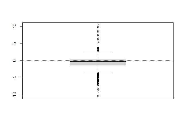
We consider samples of size $n=200$ and $n=400$ since we aim to provide a method that improves upon the maximum likelihood estimator for small and moderate sample size. For each configuration, $1000$ datasets were generated and the estimators of $\beta$ and $\gamma$ were computed through smcure and the proposed 2-step approach. We report the bias, variance and mean squared error (MSE) of the estimators, computed over the iterations for which the smcure procedure converges, in Tables 2-4. In some scenarios, mainly corresponding to the ones with $15\%$ additional censoring compared to the cure rate and smaller sample size, the iterative procedure of the EM algorithm in smcure does not converge. The most problematic setting in this regard is Model 2 scenario 3, for which $73/1000$ iterations do not converge for $n=200$ and $36/1000$ for $n=400$. The boxplots of the estimators for both methods in these non-convergent iterations are shown in Figure 1. In the other settings, only around $2\%$ or less of the iterations do not converge.

References

- [1] Aerts, M., Hens, N., and Simonoff, J. S. (2010). Model selection in regression based on pre-smoothing. J. Appl. Stat. 37, 9, 1455–1472.
- [2] Amico, M. and Van Keilegom, I. (2018). Cure models in survival analysis. Annu. Rev. Stat. Appl. 5, 311–342.
- [3] Amico, M., Van Keilegom, I., and Legrand, C. (2019). The single-index/cox mixture cure model. Biometrics 75, 2, 452–462.
- [4] Burke, K. and Patilea, V. (2020). A likelihood-based approach for cure regression models. TEST, 1–20.
- [5] Cai, C., Zou, Y., Peng, Y., and Zhang, J. (2012). smcure: An r-package for estimating semiparametric mixture cure models. Comput. Meth. Prog. Bio. 108, 3, 1255–1260.
- [6] Chen, X., Linton, O., and Van Keilegom, I. (2003). Estimation of semiparametric models when the criterion function is not smooth. Econometrica 71, 5, 1591–1608.
- [7] Cristobal, J. C., Roca, P. F., and González-Manteiga, W. (1987). A class of linear regression parameter estimators constructed by nonparametric estimation. Ann. Stat., 603–609.
- [8] Dirick, L., Bellotti, T., Claeskens, G., and Baesens, B. (2019). Macro-economic factors in credit risk calculations: including time-varying covariates in mixture cure models. J. Bus. Econ. Stat. 37, 1, 40–53.
- [9] Dirick, L., Claeskens, G., and Baesens, B. (2017). Time to default in credit scoring using survival analysis: a benchmark study. J. Oper. Res. Soc. 68, 6, 652–665.
- [10] Du, Y. and Akritas, M. (2002). Uniform strong representation of the conditional kaplan-meier process. Math. Methods Stat. 11, 2, 152–182.
- [11] Farewell, V. T. (1982). The use of mixture models for the analysis of survival data with long-term survivors. Biometrics, 1041–1046.
- [12] Ferraty, F., González-Manteiga, W., Martínez-Calvo, A., and Vieu, P. (2012). Presmoothing in functional linear regression. Stat. Sin., 69–94.
- [13] Han, X. (2017). Statistical methods for analysis of genetic and survival data with latent heterogeneity. Ph.D. thesis, New York University.
- [14] Kuk, A. Y. and Chen, C.-H. (1992). A mixture model combining logistic regression with proportional hazards regression. Biometrika 79, 3, 531–541.
- [15] Legrand, C. and Bertrand, A. (2019). Cure models in cancer clinical trials. In Textbook of Clinical Trials in Oncology. Chapman and Hall/CRC, 465–492.
- [16] Li, C.-S. and Taylor, J. M. (2002). A semi-parametric accelerated failure time cure model. Stat. Med. 21, 21, 3235–3247.
- [17] Lopez, O., Patilea, V., and Van Keilegom, I. (2013). Single index regression models in the presence of censoring depending on the covariates. Bernoulli 19, 3, 721–747.
- [18] López-Cheda, A., Cao, R., Jácome, M. A., and Van Keilegom, I. (2017). Nonparametric incidence estimation and bootstrap bandwidth selection in mixture cure models. Computational Statistics & Data Analysis 105, 144–165.
- [19] López-Cheda, A., Jácome, M. A., and Cao, R. (2017). Nonparametric latency estimation for mixture cure models. Test 26, 2, 353–376.
- [20] Lu, W. (2008). Maximum likelihood estimation in the proportional hazards cure model. Ann. I. Stat. Math. 60, 3, 545–574.
- [21] Lu, W. (2010). Efficient estimation for an accelerated failure time model with a cure fraction. Stat. Sin. 20, 661.
- [22] Meeker, W. Q. (1987). Limited failure population life tests: application to integrated circuit reliability. Technometrics 29, 1, 51–65.
- [23] Müller, U. U. and Van Keilegom, I. (2019). Goodness-of-fit tests for the cure rate in a mixture cure model. Biometrika 106, 1, 211–227.
- [24] Musta, E., Patilea, V., and Van Keilegom, I. (2022). A presmoothing approach for estimation in semiparametric cox mixture cure models. Bernoulli (to appear).
- [25] Othus, M., Barlogie, B., LeBlanc, M. L., and Crowley, J. J. (2012). Cure models as a useful statistical tool for analyzing survival. Clin. Cancer Res. 18, 14, 3731–3736.
- [26] Parsa, M. and Van Keilegom, I. (2022). Accelerated failure time vs cox proportional hazards mixture cure models: David vs Goliath? Stat. Papers (under revision).
- [27] Patilea, V. and Van Keilegom, I. (2020). A general approach for cure models in survival analysis. Ann. Stat. 48, 4, 2323–2346.
- [28] Pedrosa-Laza, M., López-Cheda, A., and Cao, R. (2022). Cure models to estimate time until hospitalization due to covid-19. Appl. Intell. 52, 1, 794–807.
- [29] Peláez, R., Cao, R., and Vilar, J. M. (2021). Nonparametric estimation of the probability of default with double smoothing. SORT-Statistics and Operations Research Transactions, 93–120.
- [30] Peláez Suárez, R., Cao Abad, R., and Vilar Fernández, J. M. (2021). Probability of default estimation in credit risk using a nonparametric approach. Test 30, 2, 383–405.
- [31] Peng, Y. and Dear, K. B. (2000). A nonparametric mixture model for cure rate estimation. Biometrics 56, 1, 237–243.
- [32] Peng, Y. and Yu, B. (2021). Cure Models: Methods, Applications, and Implementation. Chapman and Hall/CRC.
- [33] Stringer, S., Denys, D., Kahn, R. S., and Derks, E. M. (2016). What cure models can teach us about genome-wide survival analysis. Behav. Genet. 46, 2, 269–280.
- [34] Strzalkowska-Kominiak, E. and Cao, R. (2014). Beran-based approach for single-index models under censoring. Comp. Stat. 29, 5, 1243–1261.
- [35] Sy, J. P. and Taylor, J. M. (2000). Estimation in a cox proportional hazards cure model. Biometrics 56, 1, 227–236.
- [36] van der Vaart, A. W. and Wellner, J. A. (1996). Weak convergence and empirical processes. Springer Series in Statistics. Springer-Verlag, New York. With applications to statistics.
- [37] Van Geloven, N., Van der Veen, F., Bossuyt, P., Hompes, P., Zwinderman, A., and Mol, B. (2013). Can we distinguish between infertility and subfertility when predicting natural conception in couples with an unfulfilled child wish? Hum. Reprod. 28, 3, 658–665.
- [38] Van Keilegom, I. and Akritas, M. G. (1999). Transfer of tail information in censored regression models. Ann. Stat. 27, 1745–1784.
- [39] Wycinka, E. and Jurkiewicz, T. (2017). Mixture cure models in prediction of time to default: comparison with logit and cox models. In Contemporary Trends and Challenges in Finance. Springer, 221–231.
- [40] Xu, J. and Peng, Y. (2014). Nonparametric cure rate estimation with covariates. Can. J. Stat. 42, 1, 1–17.
- [41] Yamaguchi, K. (1992). Accelerated failure-time regression models with a regression model of surviving fraction: an application to the analysis of “permanent employment” in Japan. J. Am. Stat. Assoc. 87, 418, 284–292.
- [42] Yilmaz, Y. E., Lawless, J. F., Andrulis, I. L., and Bull, S. B. (2013). Insights from mixture cure modeling of molecular markers for prognosis in breast cancer. J. Clin. Oncol. 31, 16, 2047–2054.
- [43] Zhang, J. and Peng, Y. (2007). A new estimation method for the semiparametric accelerated failure time mixture cure model. Stat. Med. 26, 16, 3157–3171.