Symmetric configuration spaces of linkagesVolume: Volume , Number 0,
Abstract.
A configuration of a linkage is a possible positioning of in , and the collection of all such forms the configuration space of . We here introduce the notion of the symmetric configuration space of a linkage, in which we identify configurations which are geometrically indistinguishable. We show that the symmetric configuration space of a planar polygon has a regular cell structure, provide some principles for calculating this structure, and give a complete description of the symmetric configuration space of all quadrilaterals and of the equilateral pentagon.
Key words and phrases:
configuration space, workspace, robotics, mechanism, linkage, kinematic, symmetry2020 Mathematics Subject Classification
Primary 70G40; Secondary 57R45, 70B151. Introduction
The mathematical theory of robotics is based on the notion of a mechanism consisting of links connected by flexible joints. More precisely, a linkage is a metric graph, with edges (of fixed lengths) corresponding to the links, and vertices corresponding to the joints. See [Me, S, T] and [F2] for surveys of the mechanical and topological aspects, respectively.
A central tool in studying such a linkage is its configuration space , a topological space whose points correspond to possible positionings of in the ambient Euclidean space . These spaces are useful for understanding actuations, motion planning, and singular configurations of the mechanisms (see, e.g., [FG, KTe, KTs, MT, SSBB, SSB]); in recent years, the related notion of topological complexity has been a topic of much research (see [F1] and [BGRT, BR, BK, C, D, FP, MW]).
Observe that in the standard construction of we distinguish between configurations which are functionally equivalent though formally distinct: thus if consists of a fixed platform with two identical free arms and , the two positions shown in Figure 1 are considered distinct configurations, but are functionally the same. Thus it makes sense to consider a version of the configuration space in which they are identified.

For this purpose, we introduce the notion of the symmetric configuration space of a linkage , in which points of the usual configuration space are identified if they differ by an automorphism of – which we can think of as a relabelling of vertices of which does not change its geometric relations (i.e., which vertices are connected by an edge, and the length of this edge). One should note that there are two useful versions of the configuration space of a linkage, fully reduced and reduced (depending on whether we divide the set of embeddings by all Euclidean isometries of the ambient space , or only by the orientation-preserving ones – see §2.1 below). There are also two corresponding types of symmetric configuration spaces.
Although to the best of our knowledge, the concept of the symmetric configuration space of a linkage has not appeared in the mathematical or engineering literature, it has an obvious intuitive meaning: in real life, mechanisms do not have natural labellings of their joints, and for practical purposes, the two arms of Figure 1 are indistinguishable. Of course, if each arm is used to grasp a different object, the distinction is important, which is why the usual notion of a configuration space is more generally applicable. However, for motion planning for the two-arm mechanism from rest, the symmetric configuration space is the more economical version to use.
Intuitively, each point in the symmetric configuration space can be thought of as instructions for specifying a rigid configuration of a real-life linkage in the ambient space (), without labelling links or joints which are indistinguishable in the abstract mechanism .
Another possible application is to molecules with structural symmetries, whose reduced configuration space represents the mutual positions of their constituent atoms in space (the fully reduced configuration space does not distinguish between the two chiralities, if they exist). See, e.g., [HS, Ch. III].
Our main results in this paper are concerned with the planar configurations of the closed chain with links. On a theoretical level, we provide a systematic approach to describing an equivariant cell structure on the configuration space of a closed chain under action of the group of automorphisms of the linkage:
Theorem A.
The reduced configuration space of an -gon in the plane has a regular -equivariant cell structure, subordinate to the standard regular cell structure, and similarly for the fully reduced configuration space.
See Theorem 5.3 and Corollary 5.4 below. From the equivariant cell structure for these two types of configuration space we can then derive directly an induced (ordinary) cell structure for the two types of symmetric configuration space.
The symmetric cells of the configuration space – that is, those fixed under various subgroups of – play a central role in describing the cell structure of two types of symmetric configuration spaces, and we show:
Theorem B.
The fixed point set of the fully reduced configuration space of a planar polygon under a subgroup of is a disjoint union of components (indexed by the discrete set of configurations fixed under itself), each of which fibers successively over intervals or tori.
The remainder of the paper is devoted to two specific calculations. We show:
Theorem C.
The reduced symmetric configuration space of a planar quadrilateral is homeomorphic to a closed interval, a circle, a wedge of a circle and a segment, or a circle with its diameter.
See Theorem 3.3 below, where the cases in which each value obtains are described in full.
Proposition D.
The fully reduced symmetric configuration space of the planar equilateral pentagon is homeomorphic to a closed disc.
See Proposition 8.1 below.
1.1. Organization and main results
In Section 2 we review the main notions needed to define the various types of configuration spaces of a mechanism, and introduce the corresponding versions of symmetric configuration spaces. Simple examples of symmetric configuration spaces are given in Section 3, including a full description of planar quadrilaterals (with the details appearing in Appendix A). In Section 4 we recall some general facts about the configuration spaces of planar polygons in general, including their cell structure. Section 5 is devoted to the automorphisms of planar polygons , culminating in Theorem 5.3. Section 6 discusses symmetric configurations for planar polygons – that is, the fixed-point sets of the configuration space under various subgroups of . Section 7 shows how these general results may be applied to obtain an equivariant triangulation of one non-equivariant cell, in the case where is the equilateral hexagon. Finally, Section 8 provides a full description of the fully reduced symmetric configuration space of the equilateral pentagon.
2. Configuration spaces
We first recall some general background material on the construction and basic properties of configuration spaces. This also serves to fix notation, which is not always consistent in the literature.
Definition.
Consider an abstract graph with vertices and edges (with no loops or parallel edges, but not necessarily connected). A linkage (or mechanism) of type is determined by a function specifying the length of each edge in (subject to the triangle inequality as needed). We write for the vector of lengths.
The configuration space of the linkage is the metric subspace of (a real algebraic variety), where the map is given by . A point is called a configuration of . Note that is a subspace of the space of embeddings of in (without collisions).
2.1. Isometries of configuration spaces
The group of isometries of the Euclidean space acts on the space . Taking this action into account allows us to reduce the dimension of without losing any interesting information, as follows:
If we choose a fixed vertex of as its base-point, the action of the translation subgroup of on is free, so its action on is free, too, and we might reduce the degrees of freedom of by considering its quotient under this action.
However, such a choice will not fit in with our notion of symmetries, so for our purposes it is more convenient to think of the coordinate frame with the barycenter of a given configuration at the origin. We therefore define the pointed configuration space for to be the quotient space under translations. Thus , and a pointed configuration (i.e., an element of ) is simply an ordinary configuration expressed in terms of a coordinate frame for with the barycenter at the origin. Essentially, this means replacing the Euclidean ambient space by the corresponding affine space, equipped with a chosen direction for each axis.
If we divide by the action of the group of orientation-preserving isometries of the ambient space , we obtain the reduced configuration space of , denoted by . When has a rigid “base platform” of dimension , the action of is free. For example, if , we may fix a vertex and a link in starting at , and let assign to a configuration the direction of . The fiber of is .
Dividing by the full group of all isometries of we obtain the fully reduced configuration space of . Note that any configuration whose image is contained in a line is fixed under reflections in that line, so the action of may not be free. Thus is not generally isomorphic to . Nevertheless, is the most economical model for most linkages .
2.2. Normalization
Note that the image of a configuration is the same as the image of for any automorphism of the linkage (that is, a relabelling of the vertices preserving adjacency and edge length). This does not mean that we have an isometry of taking to – e.g., when is a bouquet of circles (closed chains), we may reflect one of them, leaving the rest in place (see also Figure 1).
However, when has a rigid “base platform” of dimension , as above, we can identify with : that is, every configuration in can be normalized uniquely to a reduced configuration , by placing the platform in a standard direction and moving the barycenter of to the origin. This will be denoted by , where the specific transformation used to normalize may not depend continuously on , but is continuous, thus providing a canonical section for the quotient map .
Any polygon in the plane always has such a rigid platform, so when is equilateral, a reduced configuration is completely determined by the orientation (that is, a cyclic ordering of the vertices ) and the sequence of angles at each vertex , measured counter clockwise from to . The automorphism is simply a permutation on preserving adjacency – that is, a cyclic shift, with or without a reverse of orientation. If the orientation is preserved, , while if reverses orientation, then , since the angles should now be measured in the reverse direction.
Example 2.1.
When is an open chain of length (see Figure 4 below), . If , is a ()-torus, parameterized by . The fully reduced configuration space may be identified with a subspace of defined as follows:
For , , and we write for the version of the fully reduced configuration space in which we require the first edge not on the -axis to point downwards.
We may then define by induction on to be the subspace of given by:
Thus for we obtain a cylinder with each boundary component omitting half a circle (opposite halves at either end).
Remark 2.2.
The configuration spaces studied in this paper are mathematical models, which take into account only the locations of the vertices of , disregarding possible intersections of the edges. In the plane, there is some justification for this, since we can allow one link to slide over another. This is why this model is commonly used (cf. [F2, KM]; but see [CDR]). However, in the model is not very realistic, since it disregards the fact that rigid rods cannot pass through each other.
Note that has a dense open subspace consisting of those embeddings of which induce an embedding of the full graph (including its edges). Similarly, has a dense open subspace . In a more realistic treatment of all configurations of in , we must cut open along the complement , consisting of configurations with collisions. The precise description of a “realistic” configuration space is quite complicated, even at the combinatorial level, which is why we work here with , , and as defined in §Definition-2.1. We observe that even such a model is not completely realistic, in that it disregards the thickness of the rigid rods. See [BS2] for a fuller treatment of this issue.
2.3. Symmetric configurations
When a mechanism has internal symmetries, the various flavors of configuration spaces described above may be unnecessarily complicated: if we take into account the labelling of the vertices, the two configurations in Figure 1 are not equivalent even in the fully reduced configuration space for such a linkage, though they may be the same from a practical point of view. To overcome this discrepancy, consider the following notions:
A graph as above has a discrete group of graph automorphisms: the subgroup of the permutations on the vertex set which preserve the (undirected) edge relation. A mechanism with length function has a linkage automorphism group , consisting of those graph automorphisms which preserve lengths. The group naturally acts on on the right by precomposition: (this means that we are simply relabelling the vertices of the given geometric configuration ), and the quotient space is called the full symmetric configuration space of . This action is not generally free.
Since the action of preserves the barycenter of the configuration, we define the pointed symmetric configuration space of to be the subspace of consisting of those equivalence classes with at the origin.
However, translating by yields a canonical isomorphism
| (1) |
(since the two actions commute). This suggests two further definitions:
The reduced symmetric configuration space of is the quotient
| (2) |
while the fully reduced symmetric configuration space of is defined to be
| (3) |
Neither is canonically describable as a subspace of .
2.4. Symmetries and normalization
As noted in §2.2 above, when has a rigid base platform , every configuration in can be normalized to a reduced configuration in ; in particular, this is true when is an equilateral polygon in the plane.
Under these assumptions, acts not only on , but also on , by sending to , where we think of as a subspace of (but precomposition with may take us out of ). We then have
| (4) |
(see (2)), so that
| (5) |
(see (1)).
Remark 2.3.
Assume that the linkage has a rigid base platform of dimension as above. If no configuration of has its image fully contained in an affine subspace of of dimension , we can always choose the normalization of to be “positively oriented”. This means that we have a canonical section , so and thus .
This will happen, for instance, if and is an equilateral polygon with an odd number of links.
3. Examples of symmetric configuration spaces
We now describe a few simple examples of symmetric configuration spaces. First, note the following:
Remark 3.1.
When the graph is a chain (either open or closed), any linkage of type is determined by the sequence of lengths of the consecutive links, and a pointed configuration for is thus completely determined by a sequence of vectors in (with for ), subject to the additional constraint that in the case of a closed chain (see [F2, §1.3]).
We thus see that if we re-order the sequence , the new mechanism will have a canonically isomorphic configuration space. However, the automorphisms of need have no direct relations with those of , so the resulting symmetric configuration spaces may differ.
3.1. Open chains
When is an open chain of length , there can be at most one non-trivial automorphism of the corresponding linkage – namely, the inversion – if is symmetric (i.e., for all ).
- (i)
If , with vertices , the reduced configuration space is , with parameter equal to the angle from to , taken in the positive direction (and the fully reduced configuration space is a half circle). The -action (for symmetric ) switches and , and therefore takes to . Thus we have two fixed points (), and is an arc (with endpoints corresponding to the two fixed points).
- (ii)
If and , with vertices , then is a torus with parameters and measured as above. For symmetric , the -action takes to , with fixed points on the anti-diagonal . Since the action is generated by reflection in , if we think of as usual as a square with opposite sides identified, in we first reflect in to obtain a triangle (with corresponding to ), and then identify with to obtain a projective plane with a disc removed along – that is, is a Möbius band.
- (iii)
As noted in §2.1, in general . When and , is parameterized by . In the symmetric case, the -action sends this to , so the fixed points constitute an -dimensional subspace with . When is odd, we have no central parameter .
3.2. Triangles
When is a closed chain of length , there is only one embedding of any triangle in , up to isometry, so .
- (i)
When is scalene, is trivial, so .
- (ii)
When is an isosceles triangle, , and its action on an embedding is equivalent to reflection in the median, so
and thus and is a single point.
- (iii)
When is equilateral, is the full symmetric group, so after dividing out by the reflection we have (a cyclic group of order ), and thus , with again.
3.3. Quadrilaterals
The usual configuration spaces of planar quadrilaterals are easy to analyze in terms of the length vector . Note that must satisfy certain inequalities in order to have a non-empty (or non-trivial) configuration space – e.g., if , we must have (see [F2, Lemma 1.4])
It is easy to see that is non-trivial exactly in the following four cases:
- (1)
An equilateral quadrilateral with , – in which case (the dihedral group of order ).
- (2)
Two pairs of adjacent links have equal lengths: , – in which case , generated by the reflection exchanging the equal links.
- (3)
Each pair of opposing links has equal lengths (distinct from each other) – in which case , generated by the two interchanges of opposites.
- (4)
Two opposite links are equal (but not all four) – in which case , generated by the reflection exchanging the equal links.
3.4. Parameterizing the configuration space of a quadrilateral
When is a quadrilateral in the plane, for generic (non-equilateral) , any reduced configuration of is determined by the angle (measured counter clockwise from to ), together with the “elbow up”-“elbow down” position of – that is, whether the (measured counter clockwise from to ) satisfies , in which case , or , in which case . If or , we say is aligned and set . Note that this last case is completely determined by the value of (but may never occur, depending on the length vector .
In the equilateral case, when (that is, the edge coincides with and coincides with ), we need an additional parameter, namely, the angle between these two collapsed intervals. This suggests that the correct way to parameterize (for any planar -polygon) is to embed it into the -torus by keeping track of the angles (oriented as above) at each vertex. In this situation is the subspace of determined by the requirement that the open chain reduced configuration defined by any successive vertex angles close up and the new angle formed is equal to the remaining vertex angle parameter. This description is more wasteful than the above, but is better suited to discussing symmetries.
3.5. The reduced configuration space of a quadrilateral
By Remark 3.1, for the ordinary reduced configuration space of a quadrilateral, we may assume .
Using the method of [MT], we have the following six cases, with the reduced configuration space given in [F2, §1.3]:
- (i)
and , with .
Here if and only if or (opposing) or any linkage for which .
- (ii)
and , with .
Here if and only if (opposing).
- (iii)
and , with .
Again if and only if (opposing).
- (iv)
, with .
Here if and only if is opposite .
- (v)
, with as in Figure 27.
Here or in cases (2) or (3) respectively.
- (vi)
, with and .
Notation 3.2.
For a quadrilateral we write , , , and for the four values of in order, and assume without loss of generality that is the longest.
Theorem 3.3.
In the notation of §3.2, the symmetric configuration space of any quadrilateral is:
- (i)
A closed interval, if , , , and ;
- (ii)
A circle, if , , , and , or if .
- (iii)
A wedge of a circle and a segment, if (a parallelogram).
- (iv)
A circle with its diameter, if (a deltoid).
- (v)
A closed interval, if (an equilateral quadrilateral).
Remark 3.4.
The fully reduced symmetric configuration space is generally different from . However, for the equilateral quadrilateral , they are the identical, in fact. This is because the fully reduced configuration space is the upper half of the reduced configuration space (see Figure 29), and is then obtained from by further identifying the right and left hand sides.
Intuitively, this is because an abstract (i.e., unlabelled) configuration for a rhombus has no distinguished orientation (unlike a scalene quadrilateral, where all four angles are generally distinct, so can be oriented in the positive direction).
4. General planar polygons
When is a polygon with more than four edges, the analysis we made above (and in Appendix A) becomes more complicated, and the number of cases too large for a full description to be useful. However, it may still be possible to say something about the cell structure of the configuration space for the various mechanisms of type . Moreover, the diffeomorphism type of (as a manifold with singularities) depends generically only on inequalities among sums of subsets of (see [HR, Theorem 1.1]).
In this section, we recall a classical approach to such cell structures.
4.1. Arrow diagrams
The pointed configuration space of a closed -chain in , with length vector , may be parameterized by points in the -torus , where for a configuration , is the vector of angles between and the positive -axis. This encodes the one-to-one correspondence between a configuration of and the arrow diagram obtained by moving all vectors to the origin. See Figure 2, where (a) is a configuration of a pentagon, and (b) is the corresponding arrow diagram.

Of course, not every value of is allowed – we have two constraints,
| (6) |
to ensure that the chain is closed.
The reduced configuration space is then , with the circle acting by rotating a configuration about the origin (as in §2.1). It may be parameterized by , since we fix . In order for to be fully reduced, we also require that the first () which is not or must be .
4.2. Cells in the torus
The torus is decomposed into -dimensional cells by (the images of) the hyperplanes in given by conditions of the form or for . In any connected component of the complement of these hyperplanes, we may use any consecutive of the parameters as local coordinates for (cf. [F2, Theorem 1.3]). However, we have no control over the intersection of with , which may no longer be connected, for example, so we follow the approach of [KM], in the formulation of [P], to describe a regular cell structure on .
For this purpose it is convenient to use the homeomorphism given by , where is the real projective line. This defines a coordinate-wise identification (the -fold product), with
| (7) |
Moreover, since , the image of under is contained in .
Note that the projective special linear group acts by Möbius transformations on , and thus diagonally on . It turns out that the orbit space is isomorphic to by [KM, Theorem 4] (which is stated in terms of stable measures on , allowing one to conformally transform any arrow diagram into one with vector sum at the origin).
4.3. Cells for the configuration space of a polygon
As in [P, §1], we first note that for an -polygon (in ), with length vector , we have a dense open subset of consisting of those arrow diagrams with all angles distinct. To each such we associate a cyclic ordering of the arrows, labelled by , on the circle: that is, a coset of the symmetric group modulo the left action of the subgroup generated by the cyclic permutation . This coset is obtained from the given labelling of the arrows by the edges of by selecting an arbitrary starting point, and the action of corresponds to choosing a new starting point. See (c) in Figure 2.
Since this process respects the -action on a pointed configuration , and thus on , the map descends to , where is the corresponding dense open subset of the reduced configuration space .
The preimage under of each coset is an open cell in . Any two such cells are homeomorphic under a relabelling of the arrows, so we may concentrate on the cell corresponding to the identity permutation: thus consists of strictly convex configurations of (in the upper half plane).
To see that is in fact a regular cell (that is, homeomorphic to a ball, with a regular cell structure on its boundary), we proceed as follows (see [P, Lemma 1.2]):
Note that preserves the cyclic order of the coordinates: i.e., in the positive direction on if and only if in , and this cyclic order on is preserved by Möbius transformations. Moreover, if is any open cell in , any has pairwise distinct coordinates, so the same is true of the set . By standard facts about Möbius transformations, for each there is a unique such that , , and . It is given by:
| (8) |
which simplifies when to , with inverse
| (9) |
Moreover, the correspondence is continuous and one-to-one.
Thus we have a map , defined by
| (10) |
which is a bijection onto its image . Because preserves the ordering of the coordinates in , we see that for , is isomorphic to the affine cell
| (11) |
Since for any cyclic permutation , is isomorphic to , it is also an affine cell under the appropriate identifications.
The top cells in correspond to the various cases where two adjacent arrows in coincide, in which case the corresponding configuration is a strictly convex configuration for a closed polygon with edges, and with length vector such that for , and for . Similarly by recursion for the remaining cells in .
4.4. Cells for the fully reduced configuration space
For the fully reduced case, note that in we can also associate to an arrow diagram a coset of the symmetric group modulo the left action of the dihedral subgroup , which acts on a labelling of the arrows in by varying both the starting point and the direction in which we proceed. Since , we have a surjection , with . We call the dihedral ordering associated to .
Again, this process respects the -action on a pointed configuration , and thus on , so induces , where is the corresponding dense open subset of the fully reduced configuration space .
Note that we have a trivial double covering map , although the corresponding map has branch points at fully aligned configurations of (if they exist, as for even equilateral polygons).
Thus the preimage under of each coset is again an open cell in , doubly covered by , where . We must be more careful in analyzing the boundary , since may have branch points there.
5. Automorphisms of planar polygons
In Section 4 we summarized briefly the standard approach to describing the cell structure of the (fully) reduced configuration spaces of polygons in the plane. We now turn to a finer cell structure needed to analyze the symmetric configuration spaces. First, we note a straightforward result about , for closed chains :
Definition.
Let be the cyclic word in positive real numbers corresponding to the (ordered) length vector . The maximal number of repeating segments into which can be divided will be called the order of (so ).
If is symmetric (with respect to reversing the order from a certain starting point), we call palindromic. More generally, if after possibly omitting a single length from it becomes palindromic, we say that is reflective. Thus is palindromic, while is reflective.
Lemma 5.1.
Given a length vector a closed chain of length , the automorphism group of the linkage is
where , the dihedral group of order , is the group of symmetries of the equilateral -gon , so in particular and .
Proof.
If and is non-reflective, rotation along the repeated segment generates .
If is reflective, we have in addition a reflection in an axis which either connects two opposite vertices and (if is even and is palindromic starting at ); connects a vertex to the midpoint of an edge (if is odd and is palindromic); or connects the midpoints of two opposite edges and (if is even and is palindromic after dropping , say). If also , we have a total of possible reflections of this form. ∎
5.1. -cells
The key to understanding the symmetric configuration space is using appropriate cells for the description of the reduced configuration space , and its fully reduced version , which take into account the -action. More precisely, we decompose (or ) into open free -cells for each subgroup of – that is, open cells of the form , with the acting on the second coordinate (see [Ma]).
The highest dimensional cells in this decomposition (with ) will be those for which the action of is free (in the interior). This simply reflects the fact that generic configurations have no symmetries, if (which fails for the equilateral quadrilateral, as we see in Lemma A.7). Note, however, that the action may take an open cell to itself; to avoid this, we must subdivide it into finer (open) cells which are permuted among themselves by (acting under relabelling combined with normalization back to the reduced form).
These fine cells are determined by “breaking the symmetry” of the corresponding arrow diagram – that is, imposing an additional (open) condition which determines a unique “canonical” labelling of the vertices.
Remark 5.2.
The subgroup lattice of plays a central role in our analysis of the equivariant cell structure. Note, however, that for certain subgroups of , any configuration stabilized by are in fact invariant under a larger subgroup. Thus for example when is the equilateral hexagon, the three subgroups shaded in the lattice of subgroups of in Figure 3 will never appear as stabilizers.

Definition.
Consider an open cell for corresponding to a cyclic (or dihedral) ordering in (or ) – see §4.4.
It is convenient to think of our geometric representation of the abstract cyclic (or dihedral) ordering as a certain (fully) reduced configuration of a mechanism consisting of unit vectors emanating from the same point in the plane. Since we are only interested in the cyclic ordering, we choose a normalized representative in (respectively, ) for in which the arrow heads lie at the cyclotomic points (), suitably labelled, with .
The action of is by changing the labelling of to , and then renormalizing by applying a cyclic shift to to obtain a new permutation with (the label of ), for a cyclic ordering.
In the case of a dihedral ordering, we further normalize by requiring that appear as the label of a cyclotomic point in the upper half-plane (unless it is at , , in which case must be in the upper half-plane).
We denote the subgroup of fixing a given cyclic (or dihedral) ordering by . Thus if and only if .
5.2. Fine cells
Note that acts freely on the dense open subspace , but takes the open cell to itself. Thus the cardinality of is the number of fine cells into which we must divide .
To specify such a fine cell, we think of as a subgroup of the cyclic group (or the dihedral group , in the fully reduced case), now acting in the standard way on the regular -gon (or the cyclotomic points on the circle). Each orbit under this action imposes a (different) partition of into fine cells, defined as follows:
- (a)
If is cyclic of order , generated by
(which is always true for the reduced configuration space), then acts on (the labelling of) the cyclotomic points as a rotation by an angle of , so the orbit of under this action is , where .
For each such orbit , we define one (open) fine cell of for each element in the orbit: this consists of those configurations (angle sets) for which the angle is strictly smaller than for all .
The same rule applies for the subdivision of in into fine cells .
- (b)
If is dihedral of order (necessarily in the fully reduced case), we distinguish three cases:
- (i)
If we have an orbit with three neighboring cyclotomic points, it necessarily includes all the cyclotomic points – in other words, is the identity permutation, and the open cell is divided into fine cells. These may be distinguished by specifying for which the angle is smallest, and then further dividing this set into two subcells by the two possible orderings of and . This will determine a canonical labelling of each configuration in the fine cell , starting at the -th vertex in the direction ; similarly for the other.
- (ii)
If we have an orbit with exactly two neighboring cyclotomic points – so the whole orbit consists of such pairs () – we may again name a fine cell , say, by specifying which has the smallest angle difference between and its cyclotomic neighbor which is not in the orbit.
- (iii)
If we have an orbit with no neighboring cyclotomic points, we may name a fine cell or by specifying which has the smallest angle , as in (i).
- (i)
Definition.
For each open cell of corresponding to a cyclic ordering as above, the membrane separating two fine cells and is the subset determined by the condition
| (12) |
Similarly, for each open cell of corresponding to a dihedral ordering , the membrane separating two fine cells and is the subset determined by one of two conditions:
- (a)
If , necessarily – say, and – and is then determined by the condition
(13) - (b)
If , is determined by the condition
(14)
Theorem 5.3.
Proof.
Since the membranes are (codimension ) subspaces of the open cells in the dense open set , we may use the identifications to try to describe the membrane using the chosen affine coordinates for .
Since for , using the formula
we see that (12) takes the form:
| (15) |
(assuming for the moment that and ).
For simplicity, let (so ): writing , , and , (15) simplifies to:
| (16) |
If we further assume that (after identifying with under an appropriate relabelling of the arrows), then , , and are taken under to the corresponding coordinates in the affine cell , as in (11).
Note that if then (by the usual rational parametrization of ):
| (19) |
so (6) becomes:
| (20) |
Setting , and substituting:
| (21) |
from (9) into (20) for , we obtain two equations involving . We can solve these for and , obtaining an algebraic equation for the membrane in the variables from (17). The fine cells bounded by this membrane are therefore semi-algebraic sets inside the affine sets (thought of as open subsets of the standard affine space ), in which the equalities (12), (13), and (14), are replaced by inequalities.
We may now use Hironaka’s result on triangulating real semi-algebraic sets (see [Hi]) to obtain the required triangulation, which can be made compatible with that of the boundaries by [L]. We do so by induction on the dimension of the naive cells: the main point to keep in mind is that once we choose a triangulation for one of the fine cells, on one side of a membrane, we may reproduce it for all the others using the free action of on the interior (and the fact that this action is compatible with that on the boundary of the fine cell, which may not be free). ∎
Corollary 5.4.
For as above, the fully reduced configuration space also has a regular -equivariant cell structure, compatible with that of in Theorem 5.3.
Proof.
The -action on by reflections in the -axis generally switches two distinct cells in the regular cell structure of Section 4, thus form a double cover of a single cell in . The only cells fixed by the -action are vertices corresponding to linear configurations (with all adjacent angles or ), and these can be dealt with as in [P, §4] (see also [GP]). ∎
6. Symmetric configurations for planar polygons
In Section 5 we described a process for producing an equivariant cell structure for the (fully) reduced configuration space of a planar polygon, based on a refinement of the non-equivariant regular cell structure described in Section 4. When the -action on the fine cells is free, the orbit yields a single cell in the associated symmetric configuration space . As noted above, this will happen in the interior of the top dimensional cells. However, in the lower dimensional cells, occurring in the boundary of those with free action, we may have fixed points. From the proof of Theorem 5.3 we see that in fact we must start from the lowest dimensional cells in constructing our equivariant cell structure. Thus, we need to understand the symmetric configurations: those fixed under a subgroup of ). In particular, these will be needed in order to obtain a compatible decomposition of .
By Lemma 5.1, for any -polygon the automorphism group is either cyclic or dihedral, so the same is true for any subgroup . We must consider three cases
:
Case I. Cyclic subgroup of generated by a reflection
:
Assume first that the subgroup is generated by a reflection , in an axis of symmetry for the labels of . As noted in the proof of Lemma 5.1, this can have three forms:
- (1)
If is odd, is a reflection in a median connecting with the midpoint of , say, so ().
- (2)
If is even, may be a reflection in
- (i)
a diagonal, connecting with , say, so (indices taken modulo ).
- (ii)
a midsegment, connecting the midpoint of with that of , say, so .
- (i)
Proposition 6.1.
Let be a planar -polygon, with generated by a reflection in the axis . We then have a map from the fixed-point set, where:
- (1)
If and is a median to , is either half of , and is one-to-one.
- (2)
If and is a diagonal, is either half of , and is one-to-one except over (the subspace of chains which close up), where the fiber is .
- (3)
If is even and is a midsegment from to , is either half of , and is a double cover.
Proof.
In each case, by reflecting a given configuration for the open chain about the geometric axis of symmetry , we obtain a unique symmetric configuration for .
- (1)
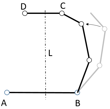
When is a median, is the -axis (the perpendicular bisector of ) in the fully reduced case. We may then rotate any configuration for about until it touches .
- (2)
When is a diagonal , say, for any configuration of the open chain we let be the line from to ; however, when these two coincide we may choose at will from .
- (3)
When is a midsegment from to , is the perpendicular bisector of ; let and be the two parallels to at distance , and then rotate any configuration for about until it touches or .
See Figure 4 for the third case. ∎
Remark 6.2.
In principle, we would like to relate the analysis of the symmetric configurations in or with the fine cell structure introduced in Section 5. This would require a better understanding of the triangulation described in Theorem 5.3. However, it is possible to use Proposition 6.1 to study the action of on the open cell of (strictly) convex configurations, under a single reflection in an axis of symmetry for the labels of .
The set of convex configurations which are fixed under must also be symmetric in the geometric sense, with axis of symmetry realizing . Such a configuration is completely described by the half on one side of , which is simply a fully reduced convex configuration for an open chain of length . As in §2.1, we parameterize such a by , (see §4.1), with
Switching to the parametrization (7), we have:
Lemma 6.3.
The set of strictly convex fully reduced configurations of a closed chain symmetric with respect to a reflection in as above are parameterized by
| (22) |
with .
The precise value of will appear in the proof.
Proof.
As in (20), we may calculate the vector sum of the arrow diagram , using the length vector for , by
| (23) |
where and .
We distinguish three cases in calculating the slope of from :
- (1)
If and is the perpendicular from to the midpoint of (because of the symmetry of ), which has length and forms an (unknown) angle of with the positive axis, so forms an angle of . Since , , and form a right triangle with hypotenuse and edge facing the angle , with . This allows us to recover , and thus and find the slope of , from which we can recover the remaining angles .
- (2)
If and is a diagonal, its direction is the vector of (23), from which we can calculate by reflecting in .
- (3)
If and is the perpendicular bisector of and , it forms an angle with , with , from which we can calculate , and thus the remaining angles .
∎
Case II. Cyclic subgroup of generated by a rotation
:
In the case where the cyclic subgroup is generated by a rotation we have:
Proposition 6.4.
Let be a planar -polygon and a rotation subgroup of , which we identify with a subgroup of for , and let . The fixed-point set is isomorphic to a disjoint union, indexed by the discrete set , of copies of , unless is collinear, in which case we replace by .
Proof.
Note that is of index in , which we identify with the automorphism group of the equilateral polygon with edges of length (unless , in which case ).
Any fully reduced configuration is determined by its restriction to an open subchain of with edges, yielding a reduced configuration for , together with a fully reduced configuration for , with equal to the distance between the start and end points of . Here must be fixed under all (geometric) rotations of , and thus under the full automorphism group , since the angles at all vertices of the polygon must be equal.
The fact that need not be fully reduced means that we will generally have two fully reduced configurations attached to each fully symmetric configuration of .
Thus for the icosagon , we have four configurations fixed under for a given (non-collinear) fully reduced open chain configuration of length , ‘attached” to the regular pentagon and pentagram on either side, as shown in Figure 5, where each of the two pairs (a)-(b) and (c)-(d) correspond to the reduced configurations .

On the other hand, the (fully reduced) -configuration for the decagon shown in Figure 5(e) is the same for , so it requires only the fully reduced open loop .
Note that even when (that is, is actually a closed loop), we still have distinct configurations corresponding to different reduced symmetric configurations : e.g., when , , the convex pentagon and the pentagram of Figure 12 correspond to two different cyclic arrangements of the petals of the bouquet of five such loops. It might be useful to think of the common endpoints of all the closed loops as an infinitesimal reduced symmetric configuration, in order to keep track of the orientations of the various loops. This is illustrated by the five closed-loop configurations shown in Figure 6, corresponding respectively to those of Figure 5, with the inner dashed symmetric configuration reduced to a point.

∎
Example 6.5.
Corollary 6.6.
For , and as above, the interior of has the same local parametrization as (see §2.1).
The case where the cyclic subgroup is generated by a rotation is in fact the only one relevant to the reduced configuration space , where we have the following somewhat simpler result:
Proposition 6.7.
If is a planar -polygon and is a rotation subgroup of , the fixed-point set is isomorphic to a disjoint union, indexed by the discrete set , of copies of
.
Case III. Dihedral subgroups
:
Let be a planar -polygon, a dihedral subgroup of , with . Choose two generators and for , which we may identify with reflections in axes and , respectively, in a regular -gon . Here we identify with a subgroup of , even though need not be equilateral, in order to have a consistent description of its automorphisms (acting on a fully reduced configuration by relabelling).
If is odd, each axis is necessarily a median (connecting a vertex of to the midpoint of the opposite edge). If is even, the axis could be a midpoint interval (connecting the midpoints of two opposite edges) or a diagonal connecting two opposite vertices.
The generator has a “basic subchain” of on which it acts by reflection in (under relabelling): this is depicted in the blue segment in either of the two diagrams of Figure 7.
When ends in a vertex (e.g., on the right in Figure 7), we have a “fundamental subchain” ( in our example), reflected under to (i.e., ), with the union of and .
When ends in the midpoint of of an edge of (e.g., on the left in Figure 7), the “fundamental subchain” ends in (so in our example), and is the union of , its reflection , and the middle segment .
Similarly, the generator has a “basic subchain” with “fundamental subchain” (given by in both diagrams of Figure 7).
Theorem 6.8.
Let be a planar -polygon and is a dihedral subgroup of , generated by reflections in axes and in a regular -gon . The fixed-point set splits as a disjoint union indexed by . For each , the corresponding component of fibers over an interval . The fiber over a value (the length of all edges of ) further fibers over a closed interval in the (the space of lines in the plane through the barycenter ). Finally, given a line in , let denote its rotation by an angle of about ; the fiber of over is then isomorphic to .
Corollary 6.9.
For , , and the two open chains and as above, the interior of has a local parametrization given by .
Proof.
Given any , let be an equilateral -gon with edge length and let be a fully reduced fully symmetric configuration for . Let and be the first two vertices of the -gon (so is at the origin, is in the positive direction of the axis, and ).
In order to determine a fully reduced symmetric configuration for (invariant under relabelling in the given subgroup ), we must choose a line through the barycenter of , which will serve as the axis of the geometric reflection realizing the action of by reflecting the labels in the “combinatorial axis” .
We let be the line through forming an angle of with (realizing geometrically the reflection in ), and let be the reflection of the origin (which is ) in the geometric axis .
Note that is the center of the circle circumscribing the regular -gon and bisects , so bisects . Since , is also on , so is also the reflection of in .

In this situation, a pair of reduced configurations for the open chains and , respectively, generally will determine (up to) four reduced configurations for the chain (the blue and yellow in Figure 7), with endpoints and (such that ).
To see how, we must distinguish two basic cases:
- (a)
If the original axis (for the reflection ) ends in a vertex , as on the right-hand side of in Figure 7, the fundamental open subchain of is , say. Let be the length of a reduced configuration for (a smooth function on the torus ). The circle of radius about generally intersects in two points and (which coincide if ). If this happens, we say that the reduced configuration of is allowable with respect to .
Allowable configurations of are defined similarly if the axis for ends in a vertex of , when the circle of radius about intersects .
- (b)
If ends in the midpoint of an edge of (of length , say), as on the left hand side of in Figure 7, let be the line parallel to at a distance of on the same side as . In this case, a reduced configuration of of distance will be allowable with respect to if the circle intersects . Similarly for if the axis ends in a midpoint.
A pair of allowable reduced configurations for the open chains and , determines a reduced configuration for the chain , by letting be one of the two intersections of the circle with , and similarly for the endpoint of .
When , we think of as the unique infinitesimal fully symmetric configuration for . We may then take to be the -axis, say. This determines , and of course, will remain at the origin.
Each reduced configuration for the chain yields a unique fully reduced configuration in the fixed-point set , by rotating about , since by comparing angles, we see that the continuation of beyond is a rotation of , and conversely. See Figure 8.

Let be an equilateral -gon with edge length and let be a fully reduced fully symmetric configuration for , as above.
Each line through determines a subspace of the pointed configuration space (a torus), consisting of all configurations for (starting at the origin) whose end-point lies on
See the right and left diagrams in Figure 7, respectively.
We let be the line through forming an angle of with , and the subspace of is defined analogously, with replacing .
To identify these subspaces, let denote the distance of the origin from , and let , where be the length vector of :
- (i)
If , clearly .
- (ii)
, then consists of a single point: the fully stretched configuration.
- (iii)
If , we see that is isomorphic to the disjoint union of two copies of the reduced configuration space , where is the closed chain having length vector : this is because for each reduced configuration , we obtain two reduced configurations by rotating about the origin so that the endpoint of lies at one of the two intersections of the circle of radius about the origin with .
- (iv)
If – that is, passes through the origin – decomposes into two complementary subspaces:
- 1.
, consisting of those configurations for which is at the origin. This may be identified with pointed configurations for the closed chain with length vector , so , where the parameter determines the rotation of the reduced configuration about the origin (see §4.1).
- 2.
, consisting of pointed configurations not ending at the origin. These are again determined by rotating any reduced configuration for about the origin, till its endpoint lies on one of the two intersections of the circle of radius about the origin with the line .
Note that is canonically isomorphic to (see §2.1), which explains how both and embed in .
- 1.
We see that given as above, the pair of configurations for and , respectively, is allowable if and only if and . Note that the maximal value of for which such allowable pairs exist is , where is the sum of the lengths of the middle edges of and (if these have an odd number of edges, as in the right picture in Figure 8). In this case, there is a unique allowable pair, yielding a fully stretched configuration for . ∎
7. Triangulating a cell for the hexagon
As noted in Remark 6.2, a full -equivariant cell structure for the fully reduced configuration space of a polygon requires a refinement of the regular cell structure of Section 5. We illustrate some of the issues involved by considering a single regular cell of strictly convex configurations for the equilateral hexagon . Note that itself is a bipyramid with six triangular facets, as in Figure 9 (in which the outer edges are to be identified pairwise as indicated).

Remark 7.1.
The vertices of are determined by a combination of symmetries and straightenings or foldings, which suffice to determine a rigid configuration. The full list of all vertices for the equilateral hexagon in the regular cell structure of Section 5 are of eleven types, depicted in Figure 10 (although, as we see in Figure 9, the same type may appear with different labellings).

7.1. The subdivided bipyramid
The bipyramid of (strictly) convex configurations for the equilateral hexagon , should be subdivided into twelve tetrahedra, which are permuted among themselves by action of on the labels. In accordance with the principles of §5.2, each tetrahedron is determined by specifying the largest of the six angles of , and then choosing which of the two angles adjacent to it should be smaller.
This in Figure 11 (on the left) we have required that the angle (labelled by ) should be the greatest, and that . One can then determine the induced inequalities , and , as indicated in the lower left corner of Figure 11.

The boundary of the tetrahedron consist of four triangular facets:
- (a)
The boundary triangle is determined by the requirement that (a straightening, which we abbreviate to in the figure), so it is an open cell of the fully-reduced configuration space of the pentagon with length vector . In turn its boundary consists of:
- i.
The edge , corresponding to the further straightening , yields a deltoid of sides and symmetry group (corresponding to the subgroup of in Figure 3, generated by the reflection in the diagonal of the hexagon).
- ii.
The edge , corresponding to the straightening yields a parallelogram of sides and symmetry group (corresponding to the subgroup generated by the rotation by ).
- iii.
The edge , corresponding to the symmetric version of the -pentagon, with -symmetry corresponding to .
- i.
- (b)
The central triangle in Figure 11 is determined by requiring invariance under the subgroup mentioned above.
- (c)
The upper right triangle is invariant under the subgroup (generated by reflection in the diagonal ), so the common edge with the central triangle has symmetry group (generated by the two reflections and thus including the rotation by ).
- (d)
The bottom triangle is invariant under the subgroup (generated by the rotation. The edge consists of configurations invariant under the subgroup of generated by the reflections in and the median connecting the midpoints of and .
Remark 7.2.
As noted above, the tetrahedron on the left of Figure 11 appears as one of twelve subcells in the bipyramid of Figure 9, obtained by a barycentric subdivision as on the right in Figure 11: specifically, the upper left facet labelled in Figure 11 is one half of the upper left facet of Figure 9, ending at the center of the lower edge of the latter (the vertex corresponding to the rectangle marked and in the former). The vertex marked in the tetrahedron is the barycenter of the bipyramid in Figure 11, corresponding to the regular hexagon configuration. Observe that all other facets of the tetrahedron are symmetric – that is, fixed under an appropriate subgroup of , as indicated in Figure 11 – and are thus internal membranes of the bipyramid, in the language of §Definition.
8. The equilateral pentagon
We now analyze in detail the case of the equilateral pentagon . Recall that [Hav, §2.4] identifies the reduced configuration space of (that is, modulo orientation-preserving isometries) as a genus oriented surface (see also [KM]), while [K] shows that the fully reduced configuration space of §2.1 is the connected sum of five projective planes. Note that Remark 2.3 applies in this case.
8.1. Cells for the pentagon
An analysis of the possible arrow diagrams for an equilateral pentagon shows that there are only four dihedral types: the first, third, fourth, and fifth in Figure 12. Note that the first and second have the same dihedral type, but different cyclic types (with reversed orientations), as we see from the corresponding configurations (which are equivalent in the fully reduced configuration space , but not in ). The fourth and sixth also have the same dihedral types, but distinct cyclic types.
In order to get a better grasp of the fine cell structure, it is convenient to use here a slightly different labelling system, corresponding to open intervals of allowable values for each of the five angles between consecutive edges (as in §3.1). We indicate the range by , and by (using the convention of §3.4). Each sequence of the form , for example, defines a unique cell, except for , which corresponds to two distinct cells as indicated in Figure 12 (where all five types are shown). The cell marked has smallest angle , while the cell marked has largest angle (with dual conditions for and ).

Note that switching all signs corresponds to reversing the cyclic order, while a cyclic shift in the sequence corresponds to a cyclic shift in the labelling. Thus (in the order in which the appear from left to right in Figure 12) we have
:
I. One (pentagonal-shaped) cell for the convex pentagon (as in Figure 14 below);
I’. An analogous (pentagonal-shaped) cell for the convex pentagon ;
II. One (pentagonal-shaped) cell for each of the pentagrams and ,
III. Five (hexagonal-shaped) cells: , , , , and , for the middle type, as in Figure 16 below).
Similarly, we have five (hexagonal-shaped) cells for the reverse order (which looks identical if we disregard the direction in which the angles are measured).
IV. Five (hexagon-shaped) cells of type , et cetera (see Figure 13)
V. Five triangular cells of type , et cetera (see Figure 17 below)
.

8.2. Boundaries of the cells
As noted above, one should think of the 32 cells constituting the reduced configuration space for the equilateral pentagon as polygonal cells (triangles, pentagons, or hexagons), identified along common edges. The edges of each such polygonal cell are obtained by a collineation: either straightening one of the angles to , or folding it to (if it was a ) or (if it was a ). Each vertex of a cell is obtained by a double collineation, corresponding to the two edges meeting at .
8.3. Symmetries of the equilateral pentagon
Each of the five types of cells corresponding to the configurations in Figure 12 are exchanged among themselves by the obvious cyclic rotations or reflections of the vertices, so only one of each type is needed for the fundamental domain of the symmetric configuration space. However, there are also symmetries acting on each cell. For example, the dashed line across the hexagon in Figure 13 represents an axis of symmetry, and indeed the two halves of the hexagon are exchanged under the reflection fixing , with and . The upper left half of the hexagon corresponds to the linear ordering of the angles , while the lower right half corresponds to ,
The cell for is a pentagon, but in this case there is a tenfold symmetry – as shown in Figure 14. Here each triangular slice of the pentagonal cell corresponds to a certain linear ordering of the angles of our equilateral pentagon (shown on the right of Figure 14). Each triangular section has one vertex at the center of the cell (the regular pentagon configuration), one at a vertex of cell (corresponding to two collineations), and one at the unique (isosceles) trapezoid configuration with one collineation, which is the midpoint of an edge. The dashed sides of each slice are obtained by changing one inequality to an equality. Compare to the subdivided bipyramid on the right in Figure 11.

The cell for (second from the left in Figure 12) is also a pentagon, similarly divided into 10 triangular regions, as shown in Figure 15.

The cell for (third from the left) is pentagonal, divided into two halves (see Figure 16), but with the bisector connecting a vertex to the midpoint of the edge opposite.

The cell for (on the right) is a triangle, similarly subdivided into two halves, as in Figure 17.

8.4. The symmetric configuration space of the pentagon
From the above discussion we see that a fundamental domain for the action of on the reduced configuration space , depicted in Figure 18, is the union of:

- (i)
One half of the hexagonal cell for of Figure 13, marked IV.
- (ii)
Attached to it along a half-edge we have one tenth of the pentagonal cell for of Figure 14, marked I.
- (iii)
Along the opposite half-edge we have another tenth of the analogous pentagonal cell for , marked II.
- (iv)
One full edge of the cell IV is glued to an edge of the half-pentagonal cell III for of Figure 16.
- (v)
Finally, the half-cell III for is glued along a half-edge to one half V of the triangle for of Figure 17.
The boundary of the fundamental domain consists of two types of segments
- a.
The two copies of each of the solid edges and are identified pairwise under appropriate symmetries. The point marked is fixed under the symmetries.
- b.
Thus we may summarize the results of this section in:
Proposition 8.1.
The fully reduced symmetric configuration space of the equilateral pentagon in the plane is homeomorphic to a closed disc.
Proof.
The fundamental domain in Figure 18 is a subspace of the fully reduced configuration space , with the inclusion. If is the quotient map, we see that is surjective, and one-to-one except along the intervals marked and in Figure 18. Thus if is the quotient map identifying the two copies of and respectively, we see that induces a homoeomorphism (since the closed disc is compact). ∎
Appendix A Configuration spaces for quadrilaterals
As noted above, the usual configuration spaces of planar quadrilaterals are well known (see, e.g., [F2, §1]). However, we need their detailed description in order to analyze the symmetric configuration spaces. Thus, in this Appendix we prove Theorem 3.3 by considering separately the six cases of §3.5
:
I. The isosceles quadrilateral case:
When is a quadrilateral in the plane with opposite edges and of equal length, we may parameterize the configurations of as in §3.4 by a subset of the angles at the four vertices, by choosing (from to ), and (from to , both measured counter clockwise). We think of as the basic continuous parameter, and note that to each value of we associate two values of , corresponding to the elbow up/down position of ( in §3.4) – see Figure 19. Note that the precise rule for calculating and from is complicated to state.

We need to understand the action of the -symmetry of (generated by the graph automorphism given by and on a configuration ). In the language of §2.4, our permutation is given by , which reverses cyclic orientation, so maps under to (where and are extraneous to determining the configuration, and may therefore be dropped). Thus the action of on takes , to as in Figure 20, with fixed points when .

Case 3.5(i) when is isosceles then may be described as follows:
Lemma A.1.
In the notation of §3.2, assume that , , , and . Then is a circle, the -action is the reflection in the diameter (with two fixed points), and thus is homeomorphic to a closed interval.
Proof.
Consider the circle of radius about a fixed point in the plane, and another circle of the same radius about a fixed point at distance from . These are the loci of allowable locations for and , respectively, if we disregard the requirement that the distance between them is . By the analysis of [MT] (see also [F2, §1]), the reduced configuration space can be described as follows in our case:
There is an arc of the circle defined as the intersection of with an annulus about , where consists of the allowable locations for with respect to . Thus the points of are precisely the possible locations for satisfying all our constraints.
For each point of , the circle of radius about generically intersects in two points and , corresponding to the elbow up and elbow down positions of (except for the two endpoints and of , for which and is flat). The angle is our parameter , with and .
By the previous discussion, the fixed points of the action of on occur when or equals . In the case illustrated in Figure 21, this happens for with its angle , and the resulting quadrilateral is not convex (on the right in Figure 19). Here is taken to be the upper intersection point of with , and is the lower point. Note that the two circles and may in fact intersect under our hypotheses as in Figure 22 (if ), but this does not affect the argument.

The constraints on , , , and ensure that there is a unique parallelogram with opposite sides and diagonals and . The angles and are then equal, and the non-convex quadrilateral is then an allowable configuration for . Since the same argument works replacing by , we have exactly two fixed points for the action of on .
The single configuration associated to the end of is the triangle with aligned (of length ). From Figure 20 we see that the -action takes it to the triangle with aligned, where is the lower edge of the arc on corresponding to (not shown in Figure 21), and the point is on the lower half of . As moves down from along , the point (the lower of the two intersections of with ) moves down, until it reaches the axis (creating the point on the right in Figure 19). We see that at this instance is on the axis, and thereafter will be in the upper half of .
Since is a simple closed curve in the torus , and the -action is topologically equivalent to the reflection of the circle in a transverse line, we deduce that is topologically a closed interval. ∎
II. Case 3.5(ii) is essentially a special case of the above:
Lemma A.2.
In the notation of §3.2, assume that , , , and . Then is a wedge of two circles, the -action switches the two circles between them (fixing the common point), and thus is homeomorphic to a circle.

Proof.
In Figure 22 the circle of radius about the midpoint of the arc now intersects in a single point (which also holds for its endpoints and , as before). The fully aligned degenerate trapezoid is fixed by the -action. Moreover, we see that the non-convex parallelograms corresponding to the fixed points described in the proof of Lemma A.1 are both identified with this degenerate trapezoid, since we have and on the right in Figure 19, and their sum equals by our assumption.
The argument in the proof of Lemma A.1 shows that the two circles corresponding to the sub-arcs and of are exchanged under the -action. ∎
III. Case 3.5(iii) becomes:
Lemma A.3.
In the notation of §3.2, assume that , , , and . Then is a disjoint union of two circles, the -action switches the two circles between them, and thus is homeomorphic to a circle.

Proof.
In this case the of Figures 21-22 splits into two disjoint arcs and , as in Figure 23, and the proof of Lemma A.2 shows that the non-convex parallelogram corresponding to a possible fixed point of the -action cannot exist. This action simply switches the two disjoint circles of between them, as before. ∎
IV. Case 3.5(iv) is similar:
Lemma A.4.
If in the notation of §3.2, is a disjoint union of two circles, the -action switches them, and is again a circle.

Proof.
In Figure 24 we choose to draw the two congruent circles and about and , so that again splits into two disjoint arcs and , as in Figure 23, and once more a non-convex parallelogram corresponding to a possible fixed point of the -action cannot exist. This action again switches the two disjoint circles of between them. ∎
V. The case of a parallelogram:
When is a parallelogram, the description of IV should be modified as follows: specializing the description of Figure 19 as in Figure 25

we now a -symmetry generated by two graph automorphisms: the first -action is given by and , and the second by and . It turns out that the first two coincide on the left (convex) configuration of Figure 25, yielding the left hand side of Figure 26. On the other hand, the first -action on the right (non-convex) configuration in Figure 25 yields the upper right hand in Figure 26, while the second yields the lower right hand quadrilateral there.

Lemma A.5.
If in the notation of §3.2 (a parallelogram), then is a union of four arcs , , , and with ends glued at and , respectively, as depicted in Figure 27. The first -action sends antipodally to , while the second -action reflects the left half of to the right half (with a fixed point at their common end ), and reflects the left half of to the right half (with a fixed point at their common end ), thus identifying with . As a result, is a wedge of the circle and a segment.

Proof.
Lemma A.6.
If in the notation of §3.2 (a deltoid) then is a union of four arcs , , , and with ends glued at and , respectively, as depicted in Figure 28, with the -action fixing the arcs and pointwise and reflecting the arc and to each other in the diameter . Thus consists of three arcs with left endpoints glued at and the right endpoints glued at .

Proof.
The analysis of Lemma A.1 shows that we have an arc of the circle with a single corresponding point on for its two endpoints and , and otherwise two distinct values. These yield the two arcs and with the -action as described. However, the fact that implies that passes through , at which point the edges and coincide, so and coincide, too, and this common edge is free to rotate about , yielding the arcs and . ∎
VI. The square:
Recall that if is an equilateral quadrilateral, the automorphism group is the dihedral group generated by the rotation (given by , , , and ), of order , and the reflection (given by with and fixed).
Lemma A.7.
In the equilateral case (), is a union of three circles of four arcs , , , and with ends glued at , , and , as depicted in Figure 29. The reflection sends to , to , to , and fixes and pointwise. The rotation sends to , to , to , to , to and to , and fixes , and . Thus consists of two arcs corresponding to and , glued at their common endpoint .

Proof.
The analysis of Lemma A.1 shows that we have two circles and with the same radius about and respectively, with . To a point on (with as parameter) there correspond two points on : one being itself (so forming a degenerate quadrilateral) and the other, , forming a parallelogram, so satisfies ). The parallelogram case corresponds to the circle in Figure 29, with at and at ). The degenerate case with corresponds to the circle , with at , while the case corresponds to the circle .
The reflection takes to , while the rotation takes to , unless in which case . Note that the two rules are consistent at and . ∎
References
- [BGRT] I. Basabe, J. González, Y.B. Rudyak, D. Tamaki, “Higher topological complexity and its symmetrization”, Alg. Geom. Topology 14 (2014), pp. 2103-2124.
- [BR] A. Bianchi & D. Recio-Mitter, “Topological complexity of unordered configuration spaces of surfaces”, Alg. Geom. Topology 19 (2019), pp. 1359-1384.
- [BS1] D. Blanc & N. Shvalb, “Generic singular configurations of linkages”, Top. & Applic. 159 (2012), pp. 877-890.
- [BS2] D. Blanc & N. Shvalb, “Configuration spaces of spatial linkages: Taking Collisions Into Account”, Bull. Kor. Math. Soc. 54 (2017), pp. 2183-2210.
- [BK] Z. Błaszczyk & M. Kaluba, “Effective topological complexity of spaces with symmetries”, Pub. Mat. 62 (2018), pp. 55-74.
- [C] D.C. Cohen, “Topological complexity of classical configuration spaces and related objects”, in Topological complexity and related topics, Contemp. Math. 702, AMS, Providence, RI, 2018, pp. 41-60.
- [CDR] R. Connelly, E.D. Demaine, & G. Rote, “Straightening polygonal arcs and convexifying polygonal cycles”, Discrete Comput. Geom. 30 (2003), pp. 205-239.
- [D] D.M. Davis, “Topological complexity of some planar polygon spaces”, Bol. Soc. Mat. Mex. (3) 23 (2017), pp. 129-139.
- [FH] E.R. Fadell & S.Y. Husseini”, Geometry and topology of configuration spaces,
- [FN] E.R. Fadell & L.P. Neuwirth”, “Configuration spaces”, Math. Scand. 10 (1962), pp. 111-118
- [F1] M.S. Farber, “Topological complexity of motion planning”, Discrete Comput. Geom. 29 (2003), pp. 211-221.
- [F2] M.S. Farber, Invitation to Topological Robotics, European Mathematical Society, Zurich, 2008.
- [FG] M.S. Farber & M. Grant, “Symmetric Motion Planning”, in Topology and robotics (Zurich, 2006), Contemp. Math. 438, AMS, Providence, RI, 2007, pp. 85-104.
- [FP] A. Franc & P. Pavešić, “Spaces with high topological complexity”, Proc. Roy. Soc. Edin., Sec. A 144 (2014), pp. 761-773.
- [GP] P. Galashin & G.Yu. Panina, “Manifolds associated to simple games”, J. Knot Theory Ramif. 25 (2016), No. 12.
- [G] R. Ghrist, “Configuration spaces, braids, and robotics”, in Braids, World Sci. Publ., Hackensack, NJ, 2010, pp. 263-304.
- [Hal] A.S. Hall, Jr., Kinematics and linkage design, Prentice-Hall, Englewood Cliffs, NJ, 1961.
- [HR] J.-C. Hausmann & E. Rodriguez, “The space of clouds in Euclidean space”, Experiment. Math. 13 (2004), pp. 31-47.
- [Hav] T.F. Havel, “Some examples of the use of distances as coordinates for Euclidean geometry”, J. Symbolic Comput. 11 (1991), pp. 579-593.
- [Hi] H. Hironaka, “Triangulations of algebraic sets”, in Algebraic geometry (Humboldt State Univ., Arcata, Calif., 1974), Proc. Sympos. Pure Math. 29, AMS, Providence, R.I., 1975, pp. 165-185.
- [HS] C. Housecroft & A.G. Sharpe, Inorganic Chemistry, 5th edition, Pearson International, London, UK, 2018.
- [K] Y. Kamiyama, “Topology of equilateral polygon linkages”, Top. Applic. 68 (1996), pp. 13-31.
- [KTe] Y. Kamiyama & M. Tezuka, “Topology and geometry of equilateral polygon linkages in the Euclidean plane”, Quart. J. Math. Oxford (2) 50 (1999), pp. 463-470.
- [KTs] Y. Kamiyama & S. Tsukuda”, “The configuration space of the -arms machine in the Euclidean space”, Top. & Applic. 154 (2007), pp. 1447-1464.
- [KM] M. Kapovich & J. Millson, “On Moduli Space of Polygons in the Euclidean Plane”, J. Diff. Geom. 42 (1995), pp. 430-464.
- [LLL] Fengling Li, Hao Li, & Zhi Lü, “A theory of orbit braids”, preprint, 2019 arXiv:1903.11501.
- [L] S. Łojasiewicz, “Triangulation of semi-analytic sets”, Ann. Scuola Norm. Sup. Pisa Cl. Sci. (3) 18 (1964), pp. 449-474.
- [Ma] J.P. May, Equivariant homotopy and cohomology theory, American Mathematical Society, Providence, RI, 1996.
- [Me] J. P. Merlet, Parallel Robots, Kluwer Academic Publishers, Dordrecht, 2000.
- [MT] R.J. Milgram & J. C. Trinkle, ”The Geometry of Configuration Spaces for Closed Chains in Two and Three Dimensions”, Homology, Homotopy & Applic. 6 (2004), pp. 237-267.
- [MW] A. Murillo-Mas & J. Wu, “Topological complexity of the work map”, J. Top. Applic. 12 (2021), pp. 219-238.
- [P] G.Yu. Panina, “Moduli space of planar polygonal linkage: a combinatorial description”, Arnold Math. J. 3 (2017), pp. 351-364.
- [S] J.M. Selig, Geometric Fundamentals of Robotics, Springer-Verlag Mono. Comp. Sci., Berlin-New York, 2005.
- [SSBB] N. Shvalb, M. Shoham, H. Bamberger, & D. Blanc, “Topological and Kinematic Singularities for a Class of Parallel Mechanisms”, Math. Prob. in Eng. 2009 (2009), Art. 249349, pp. 1-12.
- [SSB] N. Shvalb, M. Shoham, & D. Blanc, “The Configuration Space of Arachnoid Mechanisms”, Fund. Math. 17 (2005), pp. 1033-1042.
- [T] L. W. Tsai, Robot Analysis - The mechanics of serial and parallel manipulators, Wiley interscience Publication - John Wiley & Sons, New York, 1999.