Simulation analysis with rock muons from atmospheric neutrino interactions in the ICAL detector at INO
Abstract
The proposed magnetized Iron CALorimeter detector (ICAL) to be built in the India-based Neutrino Observatory (INO) laboratory aims to study atmospheric neutrinos and its properties such as precision measurements of oscillation parameters and the neutrino mass hierarchy. High energy charged current (CC) interactions of atmospheric neutrinos with the rock surrounding the detector produce so-called “rock muons” along with hadrons. While the hadron component of these events are absorbed in the rock itself, the rock muons traverse the rock and are detected in the detector. These rock muon events can be distinguished from cosmic muons only in the upward direction and can provide an independent measurement of the oscillation parameters. A simulation study of these events at the ICAL detector shows that, although reduced in significance compared to muons produced in direct CC neutrino interactions with the detector, these events are indeed sensitive to the oscillation parameters, achieving a possible precision of 10% and 27% in determining and , respectively. Hence a combination of the standard atmospheric neutrino analysis which is the main goal of ICAL, with these rock muon events, will improve the precision reach of ICAL for these parameters.
Keywords: ICAL, INO, rock muons, atmospheric neutrinos, oscillation parameters.
1 Introduction
Neutrinos as described by the “Standard Model” are massless and occur in three distinct flavours , , . Many experiments on solar [1, 2, 3, 4, 5, 6, 7, 8, 9, 10, 11], atmospheric [12, 13, 14, 15, 16], accelerator [17], and reactor [18] neutrinos have confirmed that neutrinos have mass, and the flavour states are mixtures of mass eigenstates (, , ) with different masses—this leads to the phenomenon of neutrino oscillations and is an important piece of evidence for physics beyond the Standard Model. The PMNS neutrino mixing matrix [19, 20], can be parametrized in terms of three mixing angles and a charge conjugation-parity violating (CP) phase . Some recent results from reactor neutrino experiments [21, 22] have reconfirmed the oscillations in the neutrino flavours and non-zero value of the across-generation mixing angle . Apart from this, these experiments determine the extent of mixing and the differences between the squared masses as well, although not the absolute values of the masses themselves.
There are three possible arrangements of the neutrino masses. For normal ordering, we have11 1 We have used natural units with . ; hence, and eV. For inverted ordering, with eV; hence, . In the degenerate case, . If the ordering is strong, then the ordering also determines the mass hierarchy; this problem [23] is still not solved and it is believed that upcoming experiments like the magnetized Iron Calorimeter detector (ICAL) at the proposed India-based Neutrino Observatory (INO) [24] will be able to answer this problem along with the precision of oscillation parameters. Note that the sign of (or, equivalently, the sign of ) which determines the mass ordering is still unknown, as well as the octant of . Precision experiments sensitive to matter effects during propagation of the neutrinos through the Earth can determine the sign of . Another open question regarding the neutrinos is, whether there is CP violation in the leptonic sector. Experiments such as DUNE [25] and JUNO [26] will also be sensitive to the currently unknown oscillation parameters such as the mass hierarchy and the CP phase.
The ICAL detector at the proposed INO lab will be a 51 kton magnetized iron detector with layers of iron of 56 mm thickness interspersed with active resistive plate chamber (RPC) detectors in the 40 mm air gap. It will be optimized to study muons produced in the charged-current (CC) interactions of atmospheric neutrinos with the detector. Hence it is also suitable for measuring the so-called upward-going muon flux due to CC interactions of the atmospheric neutrinos with the rock surrounding the detector (the downward-going muon flux is swamped by the cosmic ray muon background and is therefore not useful for neutrino oscillation studies) [27]. The muon loses an unknown fraction of its energy while traversing the rock to reach the detector; it still carries an imprint of the oscillations of the parent neutrino that produced it. It is therefore useful to study these upward-going or rock muons that have a characteristic signature in the detector. In this paper, we discuss the simulation studies in the ICAL detector at INO using upward-going muons and their significance. This study allows us an independent measurement of oscillation parameters.
The paper is organized as follows. In section 2, we briefly discuss the upward-going muons at the ICAL detector. In section 3, we discuss the detector response for such muons. In section 4 we discuss the main backgrounds to the rock muon events. In section 5 the detailed simulation procedure including data generation, methodology for oscillation studies and analysis are described. In section 6, we discuss the results: sensitivity to measurements of the oscillation parameters, and comparison of ICAL sensitivity with existing data [28]. We conclude with discussions in section 7.
2 Upward-going Muons at the ICAL Detector
The ICAL detector will be located under 1279 m (approx) high mountain peak and will have a minimum rock cover of about 1 km in all directions, thereby reducing the cosmic muon backgrounds [29]. Upward-going muons arise from the interactions of atmospheric neutrinos with the rock material surrounding the detector, typically within the range of 200 m (beyond this distance, the muon energy loss is so large that only very high energy muons can reach the detector, but the flux of such events is very small). These upward-going muons, also known as rock muons [30, 31, 32], provides an independent measurement of the oscillation parameters, although the sensitivity of upward-going muons to the oscillation parameters is lower than contained-vertex muons produced by atmospheric interactions inside ICAL. But an independent measurement using upward-going muon provides a consistency check with the contained vertex analysis, that results in a slight improvement of the overall measurement. This kind of analysis is helpful in any neutrino experiment.
Figure 1 shows a schematic of the processes that give rise to upward-going muons at the ICAL detector. Neutrinos, after interacting with rock, produce hadrons and muons. The hadrons get absorbed in the rock and the upward-going muons travel a distance making an angle with the -axis, and finally reach the ICAL detector. Due to the kinematics, especially at higher neutrino energies, upward-going neutrinos also (dominantly) produce upward-going muons.

The muon loses a substantial part of its energy (on the average) in the rock before it reaches the detector so the oscillation signature becomes more complicated. The formula for the average muon energy loss for muons of energy [33] produced in the rock is given by,
| (1) |
so the energy loss of the muons after propagation through a distance g/cm2 is:
| (2) |
where , is the initial muon energy, accounts for ionization losses and accounts for the three radiation processes: bremsstrahlung, photoproduction and production of electron-positron pairs. We have = 500 GeV, where both and depends on . This formula is approximate and indicative of the kind of energy loss at different energies. The actual upward-going muons have been simulated using the NUANCE neutrino generator [34] which takes into consideration the energy dependence of and as well as accounts for fluctuations. More details on the generator are given below; here we only mention that the NUANCE generator lists the vertex and energy-momentum of all the final state particles produced in CC interactions of muon neutrinos with the rock material. Hence it is possible to use the energy and direction information of the muon at the production point along with the energy loss formulae in Eqs. (1) and (2) to propagate the muon to the closest surface of the detector.
The muon energy loss depends on the distance traversed through the rock of density from the production point (vertex of the CC interaction of the muon neutrino with rock) to the detector, which we have taken to be 1 km underground. Since the muons travel essentially in the Earth’s crust (which is about 30–40 km thick on average), hence we have ; with the rock density gm/cc, as per geo-technical studies carried out by the collaboration [24].
Figure 2 (top panel) shows the energy of muons arriving at the detector from all possible upward directions as calculated from Eq. (2) using fixed values of MeV cm2/g) and cm2/g), versus the energy obtained from NUANCE for the total generated sample of 200 years exposure at ICAL. The figure shows the relative energy composition of the rock muons that reach the detector. The dependence is linear on the average, but the NUANCE points show large fluctuations, especially at lower energies which are of interest for atmospheric neutrino studies.


Figure 2 (bottom panel) shows the relative energy loss of the muon as a function of the distance travelled in the rock. It can be seen that only higher energy muons can reach the detector from further away, as expected. Each point is generated by (a) using the NUANCE value for the energy at the production point and at the detector (purple points), and (b) by using the NUANCE value at production and the energy loss formula in Eqs. (1) and 2 to determine the muon energy at the detector (green points). The difference between the two sets of points is due to the correct use of the energy-dependent values of and and also the inclusion of fluctuations, which makes a large difference at lower energies for the NUANCE points.
A substantial number of muons are absorbed before they reach the detector. Though the observed number is small, they carry important signatures of neutrino oscillations. The muon neutrino survival probability (which goes to 1 as increases) in vacuum is given by,
| (3) |
where the neutrino path length, energy and mass squared differences, , , , are in units of km, GeV and eV2 respectively. The muon neutrino survival probability in matter can be approximated by [35, 36]:
| (4) | |||||
| (5) |
Here is the (2-flavour) matter-independent survival probability, in units of eV-2 and the matter term is given by (gm/cm (GeV), also in the same units (where the signs apply to neutrinos and anti-neutrinos respectively). Here are dimensionless quantities related to the mass squared differences in matter; see Ref. [35] for more details. We have denoted the dependence on the dominant mass squared difference as : , and in the last line are coefficients independent of ; see [35, 36, 37] for details. From the last line in Eq. 5, we see that, since is positive for and negative for , hence is sensitive to the sign of the 2–3 mass squared difference via , or the neutrino mass ordering. A similar dependence is seen in the oscillation probability as well. Note that the above expressions were given in order to clarify the dependences on the various oscillation parameters; precise numerical computations for the oscillation probabilities are used in the results section.
Before we study upward-going muons for their sensitivity to neutrino oscillations, we present some details on the muon detector resolution simulation studies as well as the backgrounds to the process in the next two sections. There are three different sources of muons in ICAL. These are
- 1.
Cosmic ray muon events, where cosmic muons enter the detector from above; these constitute a major background to both the other events, viz.,
- 2.
Standard muon events, where muons arise from CC interactions of atmospheric () in the detector, with the neutrinos entering the detector from all directions.
- 3.
Rock muon events, where the muons arise from CC interactions of atmospheric () with the rock surrounding the detector; the associated hadrons produced in the interaction are absorbed by the rock and only the muons reach the detector. While these can enter the detector from all directions, they are indistinguishable from cosmic muons entering in the downward direction; hence only upward-going rock muons can be distinguished. We discuss more details about backgrounds in section 4.
3 Detector Response for Muons
3.1 GEANT4 simulation and track reconstruction
The proposed magnetized ICAL detector at INO with 1.3–1.5 Tesla magnetic field will be capable of distinguishing and which arise from CC interactions of and respectively. The ICAL detector as simulated in the ICAL GEANT4 code [38] that consists of three identical modules of dimension 16 m 16 m 14.45 m. Each module consists of 151 alternate layers of 5.6 cm thick iron plates sandwiched between glass Resistive Plate Chambers (RPCs) [39], having total mass of about 51 kton; see figure 3. The total number of RPCs for ICAL will be 29,000, each having dimensions of in the - (horizontal) plane and 35 mm thick, inserted in the 45 mm air gap between the plates.

The RPCs consist of two 3 mm thick glass plates of size approximately m2, separated by a 2 mm gap in which suitable gas flows. Copper pick-up strips of width 28 mm are mounted on either side of the glass plates, and transverse to each other, so that there are 64 strips per RPC, above and below the glass plates. A high voltage of about 10 KV is applied across the glass plates. When a charged particle passes through an RPC, it creates a discharge which generates electrons and ions that flow towards the electrodes. The electrons are picked up by the pick-up copper strips above and below the RPC and detected by the associated electronics as a pulse with nano-second timing. The pick-up strips above and below are in transverse directions thus giving the and locations of the pulse, also called a ‘hit’, while the RPC layer number in which the pulse was detected gives the location of the pulse. In this way, each pulse due to a charged particle is stored as a hit, with position information in pixels of size in cm, along with the timing information; here = corresponds to the vertical direction while defines the axis which is taken to lie along the larger (48 m) length of the detector. In particular, due to the configurations of the pick-up strips, the - and - information are separately available. This information is used to determine the momentum of the muon. This is discussed later.
The magnetic field is generated by passing current through copper coils, which pass through coil slots in the plates as shown in figure 4. It can be seen that due to the coil geometry, the magnetic field is confined to the - plane (the plane of the iron). Furthermore, the magnetic field is distributed in such a way that it divides the whole ICAL into three regions. The main region is the “central region” [40] within the coils slots (with m in the central module and analogous regions in the outer modules) which has the highest, as well as most uniform magnetic field in the direction, while the magnetic field in the “side region” (outside the coil slots in the direction) is about 15% smaller and in the opposite direction. The region labelled as “peripheral region” [41] (outside the central region with m) has the most varying magnetic field in both magnitude and direction. Hence the side and peripheral regions will be affected by having a more complicated magnetic field as well as having edge effects i.e., both of them have a larger fraction of events (about 23% compared to 12% of events with vertex in the central region) where only a part of the muon trajectory/track is contained and detected within the detector.

As stated earlier, as the muon passes through the detector, it leaves a hit in each RPC that it traverses. Due to the presence of the magnetic field, the path of the muon is bent and hence the succeeding hits form a curved ‘track’ in the detector. Events are analyzed if there are at least 3 hits, and the hits are sent to a Kalman filter to determine the muon charge-sign and momentum. The Kalman filter uses the knowledge of the local magnetic field to try and fit a “track” to multiple sets of hits. Recall that the mutually transverse pick-up strips yielded information of hits in the - and - planes which can be combined to give information. The charge to momentum () ratio for each track is then determined by iterating the information of the vector containing the location of the hits, the slopes and ratio . The initial values of the location are those of the first hit; the slopes obtained from the first two hits, and set to zero initially. The GEANT4 ICAL simulation uses the magnetic field map and the detector geometry to construct a gain matrix that predicts the location of the next hit in the adjacent layer. Once it finds such a hit, it adds it to the track and carries on until it has accumulated a set of hits into a track. There can be more than one such track; the longest one is identified as the muon track. From the extent and direction of bending in the magnetic field, the muon momentum and the sign of its charge is determined. Notice that the magnetic field is mostly (in the central and side regions) along the direction; hence a charged particle travelling purely along the direction (azimuthal angle ) will not experience any magnetic force. A rock muon travelling upwards into ICAL will have and hence the -component of its momentum, . In general, the in-plane components of the momentum are also non zero. This ensures that there is a force that bends the track both in the (due to ) and (due to ) directions, thus enabling reconstruction of both (See Ref. [41] for details).
3.2 Fiducial volume and nature of tracks
Tracks are distinguished based on whether the track is completely or partially contained inside the detector, as well as whether the track starts from well within the detector or near the edges. However, note that standard muon events from CC interactions occurring near the edge of the detector may be mis-identified as either cosmic muon or rock muon events. To overcome this ambiguity22 2 This arises mainly because ICAL is a detector with layers rather than having a single volume such as in Super-Kamiokande, where the fiducial volume is actually a part of the volume of the entire detector., the fiducial volume is enumerated as follows: All events starting from, or produced in the bottom layer and in a region within 50 cm of the four (front, back, left, right) faces of the detector are considered to be rock muon events. There are rock muon events entering from above (both in the top layer and from the four sides) but they are lost in the huge cosmic muon background which is orders of magnitude larger and are ignored. Hence these rock events will contain a small fraction of standard muon events.
The following possible type of tracks exist:
- 1.
The track is completely contained within the (fiducial volume of the) detector. This indicates that a CC interaction occurred at the vertex, producing a muon that stopped within the detector. This is identified as a completely contained atmospheric neutrino or standard muon event.
- 2.
The vertex of the track is completely contained within the (fiducial volume of the) detector, but the track may itself not be fully contained. This indicates that a CC interaction occurred at the vertex, producing a muon that exited the detector. This is identified as a partially contained atmospheric neutrino or standard muon event.
- 3.
The track starts from outside the detector (the first “hit” is outside the fiducial volume) and stops inside the detector, moving in the upward direction. This is identified as a partially contained rock muon event. A sample track for such an event, entering the detector from below with GeV, and is shown in figure 5 as a function of time, while figure 6 shows the - and - projections of the original and corresponding digitised track.

Figure 5: Sample track of a 5 GeV rock with initial angle starting at the bottom of the detector in the central module. 

Figure 6: The - (lfet panel) and - (right panel) projections of the track shown in figure 5 and the corresponding digitised “hits” in cm2 pixels shown in green. Notice that the muon starts out moving in the positive direction, from the bottom of the detector ( cm) somewhere in the central region of the central module, where the magnetic field is dominantly in the positive direction; see figure 4. Since the muon has momentum components in both the positive and positive directions, the force on the (positively charged) muon due to the magnetic field bends it in the positive and negative directions. Hence the muon track, which had started out in the positive direction, bends around towards the negative direction and continues to move upwards; see the - projection of the track in figure 6. There is no force here in the direction and hence the track in the - plane is practically a straight line.
- 4.
The track starts from outside the detector (the first “hit” is outside the fiducial volume) and exits the detector, moving in the upward direction. This is identified as a through-going rock muon event. Such a sample track is shown for a 200 GeV muon entering from the bottom in the central region of the central module, with in figure 7. Since there is no initial momentum in the direction, the small changes in are due to local scattering in the detector. However, on digitisation, the track is seen to be constant in the direction, bending to the left in , as expected, and exiting the detector from the top, as can be seen in figure 8.

Figure 7: As in figure 5 for a 200 GeV muon, with starting at the bottom of the detector in the central module. Notice the very small scale in . 

Figure 8: The - (left panel) and - (right panel) projections of the track shown in figure 7 and the corresponding digitised “hits” in cm2 pixels shown in green. - 5.
When the track starts from outside the detector and is moving in the downward direction, this is identified as a cosmic muon event.
3.3 Muon track reconstruction
As has been discussed in [40, 41], ICAL has good energy and direction resolution in both the central and peripheral regions of the detector. However, these studies on muon energy, direction reconstruction and charge identification capability were performed with a view to understand the detector response for the main events at ICAL, viz., CC muon neutrino interactions inside ICAL. Hence, all these studies used a simulated data sample where the neutrino interactions occurred inside ICAL so that the produced muons were also often inside the detector.
For the current study, we need to understand the response of ICAL to muons that are entering the detector from outside. These are also very “clean” events in that there are no accompanying hadrons [43]. Hence we first calibrated the detector response to such events using a GEANT4-based [38] code to generate and propagate the events through the simulated ICAL detector. Note that the upward-going muons enter the detector through five different faces (left, right, front, back and bottom). While about half the upward-going muons have their vertices in the bottom of the detector, the four sides (left, right, front and back) of ICAL together account for the other half of the events. In each case, the muon experiences a different local magnetic field. Hence the response will be different in each case. However, muons that enter through the bottom face of the detector experience regions corresponding to all the possible choices—central, peripheral and side. Hence, we study the response of the bottom face of the whole ICAL to muons. This contains portions of the “central” and “peripheral” regions and so its response is likely to be intermediate between the two.
As the muon enters ICAL, it produces signals in the RPCs. These signals are localized to a size of 3 cm, which determines the spatial resolution of the muon track in the - and -directions and are called “hits”. An event has hits in several layers (along the -direction). Since the detection efficiency of the RPCs is 95%, there may be different numbers of - and -hits in any layer. Hence the total hits per event are then determined as the sum of the maximum value of the - or -hits for each layer. The entire set of hits in the event is passed to a Kalman filter algorithm that selects out the hits associated with the muon track, while simultaneously fitting the track to reconstruct the momentum, direction, and sign of charge, based on propagation in the local magnetic field. The hits that are rejected by the algorithm constitute the so-called “hadron hits” that are used to calibrate the associated hadron energy. Since at least three hits in two layers were required to identify a hadron shower, it was found [24] that only hadrons with energy GeV formed showers.
The selection criteria to choose or drop an event were decided so as to get reasonable fits and hence resolutions. Mainly one major selection criterion has been applied in the region to remove low energy tails; this was similar to that used in studying the peripheral muons [41]. The events were selected in a manner such that, if the track was partially contained and ended well within the detector (most likely scenario at lower energies) then it was considered for analysis, but if it was through-going (more likely at higher energies greater than about 10–15 GeV), then the event was selected only if . A somewhat looser constraint has been obtained by also taking into account the angle at which the muon enters (since the number of layers traversed and hence the number of hits in a track are dependent on this) by demanding that . This criterion removed muons that exited the detector leaving very short tracks inside, which were typically reconstructed with much smaller momenta than the true values.
This can be seen from figure 9 which explains the effect of the selection criterion on reconstructed momentum () in the region. Here, 10,000 muons with fixed input momenta and direction () were randomly generated with vertices uniformly distributed on the bottom face of ICAL, with uniform random azimuthal angle, (smeared).


It can be seen that, at lower energy ( = 5 GeV/c), the criterion does not significantly affect the momentum distribution as most of the events are fully contained. On the other hand, the hump at lower energy for = 15 GeV/c is due to the charge mis-identification which has been eliminated with the cut (In fact, the condition that only one track be reconstructed, as demanded in the peripheral muon analysis [41], was not required as the present constraint on was found to be sufficient). The resulting histogram was fitted with a Gaussian distribution to determine its width , from which the muon momentum resolution has been defined as the ratio of the width to the initial momentum ().
Note that 3 layers is the criterion for the events to be passed to the Kalman filter. All rock muon events have tracks starting from the edges or faces of the detector and hence are typed as partially contained events (defined as at least one end of the track being close to any edge of the detector). For all such events, the criterion is . For vertical events, with , this leads to a sufficiently long path length traversing about 15 layers. Since the separation between the RPCs is nearly 10 cm, this corresponds to a time difference between the first and last hits of ns. Even for horizontal angles such as (), where the muons cross only 3 layers, such a slant track would traverse a longer length of through each layer. So even if the total number of layers is less, this criterion would correspond to a total distance of about 1.5 m or ns, which is of the 1 ns timing resolution of the RPCs. In short, the criterion used ensures that the time difference between the first and last hits is sufficiently large for unambiguous up/down discrimination. We will later see the importance of this selection criteria in reducing the cosmic muon background.
The bending of the tracks determines not just the magnitude of the momentum of the muons but their direction as well. Figure 10 shows the histograms of the difference of the zenith angle at the start and end of the track for sample muon energies, for an input angle and .

It is seen from the mean and rms values that the distribution is more or less symmetric, especially at higher energies. This is because the magnetic field changes direction outside the coil slots and hence the direction of bending switches when the particle goes from a region inside the slots to a region outside (or vice versa). This is more likely to occur at higher energies when the muon traverses the entire detector and even exits it. Hence the smearing of events over the azimuthal angle dilutes the effect.
For better clarity, the zenith angle at the start and end of the track are plotted in figure 11. Shown are the distributions for two sample energies, a lower energy of 10 GeV and a higher one of 100 GeV for fixed value of input zenith angle, , generated in the central region of the detector and so the magnetic field is initially in the direction. Here the events with azimuthal angle are selected so that the component of the particle momentum along the axis is always positive. It can be seen that the reconstructed zenith angle is always larger than the input value because negative muons were generated. This separation is much less at 100 GeV than at 10 GeV. This bending allows for the reconstruction of the muon momentum and the sign of its charge. As can be seen from the sample tracks shown in figures 5, 6, 7 and 8, the average values of are not really reflective of the detailed bending of the track which is complex and depends on the charge-sign of the muon, the (variable) magnetic field components in the local region of the track, and the momentum components of the incoming muon. All these affect the reconstruction and charge identification efficiency and the muon momentum resolution, which we discuss in the next section.


3.4 Reconstruction Efficiency and Resolution of Muons
Now we discuss the results on reconstruction efficiencies and energy and angular resolutions for the muons based on the selection criteria discussed earlier. Figure 12 shows the reconstruction and charge identification efficiencies in the bottom region of ICAL.
The reconstruction efficiency, which is defined as the ratio of the number of GEANT4-simulated events reconstructed to the total events simulated, was found to be greater than 85% for energies less than 50 GeV and for angles greater than . The relative charge identification (cid) efficiency, which is the ratio of the number of events with correctly identified muon charge sign to the total number of reconstructed events, is better than 95%, and in fact nearly 97% for GeV; it is better than 85% for upto 150 GeV and .


Figure 13 shows the muon momentum resolution and the zenith angle resolution. The detector can optimally detect muons with about 10–12 GeV energy at all angles. Muons with higher energy can exit the detector and hence the resolution decreases beyond this point. Note that the zenith angle resolution is the value of the width of the fitted Gaussian distributions in radians.


The muon resolutions are better than about 20% for muon energies less than 50 GeV and for angles greater than , and worsen for larger energies and angles but remain less than 50% upto GeV. The resolution, which was about a degree for few GeV region, is similar to that obtained from earlier studies [41]. We shall use these values of muon reconstruction efficiency and resolution in our simulation studies of upward-going muons in the next sections. Before doing this, we list the main backgrounds to the process of interest, and methods of reducing them.
4 Main backgrounds
Upward-going rock muons can enter the detector from the bottom of ICAL, from the front and back, as well as from the sides (left and right faces). While the events from the side are the least, there are roughly equal number of events from the bottom and the front-back due to the detector dimensions of .
The primary criterion for identification of these rock muons is the ability to distinguish up- and down-going muons since the down-going muons are primarily cosmic ray muons. The RPC timing is crucial for this purpose; the RPCs that have been designed and tested by the collaboration have a timing resolution [24] of about 1 ns. Since the vertical spacing between RPCs is 9.6cm, a minimum of hits in at least three layers is required to unambiguously determine from the timing information whether the muon was an up-coming or down-going one; in fact, the Kalman filter algorithm that identifies and fits the muon tracks requires hits across at least 5 contiguous layers (although one or more layers may not have a hit in them). Earlier GEANT4-based [38] simulation studies [40] by the collaboration have shown that the fraction of tracks which are reconstructed in the wrong direction (upward tracks being identified as down-going and vice versa) varies from 1.5–4% for muons with GeV and with zenith angles from –0.2, with worse reconstruction for larger angles as expected. This fraction decreases to less than 0.3% for large angles of when the energy increases to 2 GeV. Hence the probability of muons with energies GeV being reconstructed in the wrong direction is very small and will be ignored. The additional selection criterion described above plays an important role.
These upward-going muons are to be discriminated from two other types of events which form the background to this measurement. First, are those atmospheric neutrino events that produce muons through CC interactions inside the ICAL detector and are a part of the main studies of ICAL; we label them as “standard muons”. The other background is due to the cosmic ray muons. We first consider the “standard muons” produced in CC interactions inside ICAL.
4.1 Standard Muon background
Rock muon events give rise to muon tracks that start at the edges of ICAL. Note, however, that (up-going) atmospheric neutrinos producing muons via CC interactions at the edges of the detector can be mistaken for rock-muon events since their tracks also begin at the detector edges. The number of rock muon events depends on the aperture, i.e., the area of the surface exposed to these muons. In contrast, the number of CC “standard muon” events depends on the volume of detector in which they are produced. This background can be significantly reduced by suitable selection criteria as we describe below.
Bottom events
: Figure 14 shows the rock events entering from below, through the bottom of ICAL (so-called “bottom rock events”) that are detected, starting from the bottom-most RPC layers. Atmospheric neutrinos that interact with the nucleons via CC interactions in the bottom-most layer of ICAL also produce muons that are detected, starting from the bottom-most RPC layer. Among these events, those which are detected as single tracks (identified as muons) having no visible accompanying hadronic activity and produced in the upward direction, can mimic the rock events. Hence such CC atmospheric muon neutrino events form an irreducible background to the “bottom rock events”. These are also shown in figure 14. The standard muon background satisfying the above selection criteria is about 2.5% of the bottom-rock events at muon energies of GeV, and falls off to 0.5% (%) at () GeV. We therefore apply a selection criterion of GeV in order to reduce this background to less than 2.5%.
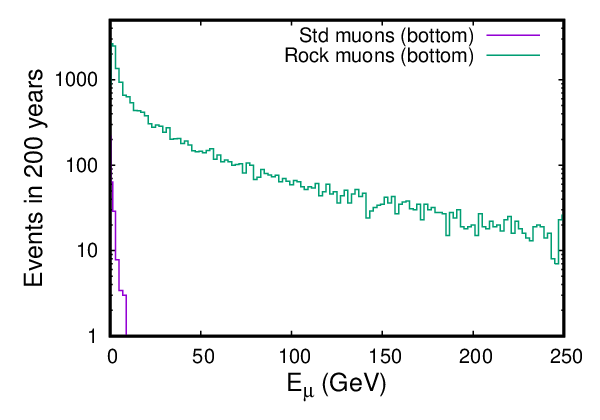


Front/Back events
: Similarly, the up-going atmospheric neutrinos that produce up-going muons in CC interactions at the edge of the front and back faces of ICAL with no visible associated hadronic shower, can mimic rock muon events arriving through the front and back faces of the detector. Depending on the direction () of the muon, it can traverse a large distance before reaching an RPC layer and giving a “hit” there. For instance, a muon at angle can traverse cm before reaching an RPC layer. Hence, we have assumed that any muon track whose first hit is within 50 cm of the detector faces (front, back) can be considered to be a rock muon event. This means that all standard muons produced due to CC neutrino interactions in the iron material within 0.5 m of the edges form an irreducible background to the rock muon events. This is in contrast to muons entering from above or below where they meet an RPC layer just adjacent to the top or bottom iron layer and hence this irreducible background is relatively larger at low energies, being 47%, 11%, and 2% of the front- and back-entering rock muon events at 1, 4, and 10 GeV respectively. The larger background is because these interactions occur in 150 layers of of iron, which is much larger than the interactions occurring in one bottom layer of dimension ; see the schematic of the ICAL detector in figure 3. The rock muons entering the front face of the ICAL detector has also been shown. Here, we apply a selection criterion of GeV to reduce this background from the front and back faces to less than 10%.
Left/Right events
: Lastly, the atmospheric neutrinos entering from the side (left and right faces) of ICAL can interact via CC interactions to again produce muons within 50 cm from the detector edges, thus mimicking rock muon events entering from the sides. These backgrounds amount to 20%, 3%, and % for muons with energies and 10 GeV. Again we employ a selection criterion of GeV to reduce this background from the left and right faces to less than 3%.
Fiducial volume
: We note that the choice of fiducial volume for rock muon events of GeV muons produced within 0.5 m from the front, back, left and right edges and the events with GeV produced in the entire bottom layer, is quite conservative, especially since it is blind to the direction of the muon, and a smaller value may cut down the CC neutrino events further. In the absence of any available studies in this regard, we retain this conservative choice. In our further analysis, we have chosen to ignore these background events as being small. It is possible to actually carry out the detailed analysis including these background events, but that is beyond the scope of this work.
4.2 Cosmic Muon Background
The second kind of background arises from the cosmic ray muon events produced in the Earth’s atmosphere that directly leave tracks in the ICAL detector. These form the main background to all muon events (CC atmospheric muon neutrinos producing muons as well as rock muon events) in the ICAL detector. In particular, those cosmic muons that are mis-identified in their direction (down-going cosmic muons mis-identified as being up-coming ones) form the cosmic muon background to rock muon events. These can be partially eliminated from the rock muon sample by imposing an angle cut that allows only upward-going muons for the analysis since there are no cosmic ray muons arriving from below. As a matter of abundant precaution, we also reject up-going muons that enter at angles larger than .
Note that the decision of an event being up-going or down-going depends on the ability of the detector to discriminate up and down events (that is, the probability to reconstruct a true angle as which results in reconstructing with the wrong sign. In our simulations studies, we have used a sample of 10,000 muons of fixed energy and direction. We have already mentioned earlier that the selection criteria result in a track length of the muons which corresponds to a time of 5 ns or more. Since this is 5 standard deviations away from the RPC resolution of 1 ns, only an event in a million is expected to be reconstructed in the wrong direction; these are unobservable in a sample size of 10,000 that we have used for the analysis. Generating millions of events and analyzing them in GEANT is a slow and difficult process, and is also limited by the memory space available on the computer. However, the cosmic muon flux is huge and so even a small number of these events, mis-identified in direction, can form a significant background to the rock muon events. In order to accurately estimate the background from these events, it is therefore necessary to find the fraction of up-down mis-identified cosmic muon events using a different approach.
To this end, a Monte Carlo program was written, that generated cosmic muon events according to the fluxes given in Ref. [33]. Since the peak height below which INO is proposed to be located is 1.3 km (approx), and the access tunnel to reach this cavern is 2.1 km long, the simulation assumed a simplistic conical mountain33 3 This reflects the true mountain profile quite well, and overestimates the muon fluxes from the West () where the mountain meets a plateau. with height 1.3 km and radius of base of 2.1 km. Cosmic muons produced on the surface were propagated (based on their energy and direction) to the detector, using the energy-loss formula of Eqs. (1), (2). These muons were then propagated inside the detector assuming no magnetic field, for simplicity, and the corresponding hits/tracks analyzed. Since the fluxes are very large, about 4000 events per hour, it was feasible to only generate events for 73 days, about 1/5th of a year. Of the 6527940 cosmic muon events with energy GeV, 264803 events did not satisfy the criteria of hits in at least 3 layers and were eliminated. A further 248059 events did not pass the selection criteria of . The remaining events were multiplied by 50 to obtain events for 10 years and sorted into three sets.
The first set corresponded to those events with , in which the time difference between the first and last hits is –6 ns. The second set corresponded to those events with , in which the time difference between the first and last hits is –7 ns. The final set corresponds to those events which have , in which the time difference between the first and last hits is ns. The total events in each set is given in Table 1. The direction mis-id fraction of events can then be estimated using the probabilistic approach: one in events with –6 ns (5–6 deviation in timing), one in events with –7 ns (6–7 deviation), and none for events having greater than ns. It can be seen from Table 1 that just 13 cosmic ray background events can be expected in 10 years. We therefore ignore this background as well.
| Event Set | Events in | Probability of | Direction |
|---|---|---|---|
| ns | 10 years | direction mis-id | Mis-id’ed Events |
| 5–6 | 22349400 | 12.8 | |
| 6–7 | 4558600 | ||
| 291798500 | 0 | 0 |
Recently, the INO collaboration has measured [44] the direction mis-identified events in the cosmic ray muon sample detected in the prototype mini-ICAL detector functioning in Madurai, South India. The mini-ICAL detector is a m2 scaled prototype of ICAL, about 1 m high, with 11 iron layers, with RPCs populated only in the central m3 volume. Hence the muons detected are purely cosmic ray muons and are all expected to reconstruct in the downward direction. While the paper includes a detailed analysis of improving time and position resolutions of the RPC detectors, the direction mis-identification fraction has also been studied by them for various selection criteria. The results are presented for tracks with hits in different number of layers (–10), with no selection criteria analogous to the used here. However, since the cosmic muons peak around (), we can roughly compare these results with our probabilistic approach by assuming . Using the argument above, we then have the statistical probability of direction mis-identification with to be 0.020%, 0.008%, 0.003%, and 0.001% respectively. The measured results with reasonable selection criteria were found to be 0.140%, 0.014%, 0.0035% and 0.0014% respectively, the latter with larger errors; see Ref. [44] (and figure 22 therein) for more details. This agrees with the probabilistic estimates, especially for larger and thus validates our estimates.
4.3 Other backgrounds
Finally, it is possible that down-going cosmic ray muons that do not interact in the detector interact with the rock below the detector to give up-going neutrons and pions that are detected in ICAL. A study by the MACRO collaboration [45] has found that the background from such events is about 1% with a flat zenith angle distribution. Although the actual number of events depends on the details of the detector sensitivity and depth at which it is located, this gives a ball-park estimate since the sizes of MACRO and ICAL are commensurate. Such hadrons generally shower and will be rejected by the track-finding algorithm that fits muon tracks. Hence it is expected that these events will not constitute a significant background to the rock muon events.
In summary, there are different backgrounds to the study of rock muon events, and they can be reduced by a judicious choice of selection criteria. The background due to CC atmospheric neutrino events from the front and back of the detector forms the largest background. However, in the analysis that follows, we have assumed that the backgrounds can be kept under check and have not included the impact of these on our results. There is certainly room for improvement here but this is beyond the scope of this simplistic analysis. We discuss the physics analysis of upward-going muons in the next section.
5 Physics Analysis of Upward-going Muons
5.1 Event Generation
We have used the neutrino event generator NUANCE (version 3.5) [34] to generate (unoscillated) events corresponding to an exposure of 51 kton 200 years (i.e., 200 years’ at ICAL) of unoscillated upward-going muons in the energy range 0.8–200 GeV. The atmospheric neutrino fluxes as provided by Honda et al. [46] at the Super Kamiokande experiment [47] were used. The ICAL detector specifications were defined inside NUANCE. Dimensions of the detector were chosen such that no events were generated inside the detector i.e., only its external geometry was used. The actual material in which interactions occur is rock, whose density was taken to be 2.65 gm/cm3. To cut off cosmic ray backgrounds, only events arriving with zenith angles44 4 Note that rock muons are produced in the rock surrounding the detector so that they can enter the detector from above, below, or any of the four sides. The ones entering from above are lost in the huge cosmic ray muon background and cannot be detected. Hence here we only detect rock muons entering from the bottom and sides of the detector. (), were selected [48]. The NUANCE generator itself propagates the muons produced in the CC interaction to the closest surface of the ICAL detector by using appropriate energy loss formulae as discussed earlier in Eqs. (1) and (2). The hadrons are absorbed in the rock and so only muons enter the detector. The NUANCE generator gives information not only of the initial vertex of the CC neutrino interaction but also the energy and direction of the initial neutrino and the produced muon. The information on the neutrino energy and zenith angle is saved for later use to oscillate the data set according to the neutrino oscillations.
Two data sets were generated: set I with “normal” fluxes, and set II with “swapped” fluxes where the muon and electron neutrino fluxes were interchanged. This was used to enable incorporation of oscillations later. Note that the energy and direction of the neutrino initiating the event is also available in NUANCE. These values are required to generate the correct neutrino oscillation and survival probabilities, as described later. The information on the vertex and energy and direction of the produced muons is used to propagate the muons to the detector surface, as described earlier. Only those events falling within the aperture of the detector are retained; hence generating rock muons is a time-consuming process in contrast to the “standard” analysis where the CC interaction occurs inside the detector itself.
The number of muon events from the two channels are generically given by,
| (6) | |||||
| (7) | |||||
The label ‘t’ refers to the true values of the muon energy and zenith angle; is the exposure time and is the total number of target nucleons in the rock, which is assumed to surround the detector to an infinite distance in all directions. The produced muons are then propagated [34] in the rock with suitable energy loss until they reach the detector. In order to speed up the events generation, two quantities can be specified: the minimum energy of the muon when it reaches the closest face of the detector, and the maximum zenith angle ; the latter prevents the generation of the uninteresting horizontal and down-going events. Here and are the atmospheric fluxes of and respectively and similar equations hold for produced from CC interactions of muon anti-neutrinos.
Instead of being passed through GEANT, the muon energy and angle corresponding to these NUANCE events were then smeared according to the resolutions and reconstruction efficiencies obtained in section 3.4 so that the event was binned according to its smeared/observed energy and angle values. Neutrino oscillation is then applied as follows.
The set of input neutrino oscillation parameters used in the analysis are listed in Table 2. Since the analysis is not sensitive to the 1–2 parameters, these were kept fixed throughout. In addition, these events are not sensitive to the CP phase, which was also kept fixed. The normal ordering was assumed to be the true one as well.
| Parameter | Central/input values | 3 ranges |
| (eV2) | 7.5 | fixed |
| (eV2) | 2.4 (NH) | [2.1, 2.6] (NH) |
| 0.304 | fixed | |
| 0.5 | [0.360, 0.659] | |
| 0.022 | [0.018, 0.028] | |
| (0) | 0 | fixed |
Due to the presence of both and atmospheric fluxes, there are contributions from two channels, viz., the survived neutrinos, determined by and the oscillated neutrinos, determined by , to the muon events in ICAL. Hence each event in set I is oscillated according to as determined by the oscillation parameters, while each event in set II is oscillated according to .
To implement oscillations we have used a re-weighting algorithm as follows. We generated a uniform random number between 0 and 1; if , then the event survives oscillations and is binned appropriately; similarly, if we considered the swapped event to contribute as an oscillated event. Events from both channels were added to get the total events. Symbolically, we have:
| (8) |
A similar procedure was applied to get events from , with the corresponding anti-neutrino survival/oscillation probabilities.
Note that , as can be seen from figure 15 where the relevant survival and oscillation probabilities for both neutrinos and anti-neutrinos have been plotted for two different values of the zenith angle, [50].
The oscillated data was binned into bins of observed/ smeared muon energy and bins. We have used two schemes of binning in this paper. Firstly, since there were substantial events with energy GeV, we took 25 bins of smeared energy as given in Table 3; we refer to this as exponential binning. The energy bins were optimized such as to obtain reasonable number of events in each bin. Secondly, we took linear energy bins with the width of 1 GeV from 1–45 GeV for comparison with exponential binning scheme to check sensitivity to oscillation parameters. The data sample has a proportionately larger component of higher energy events which were not sensitive to oscillations, so finer bins were used at lower energy. In each case, the data was divided into seven bins of from 0 to 1; 6 uniform ones of width 0.15, with the last bin from 0.9–1.0.


| Energy range (GeV) | Bin width (GeV) | No. of bins |
|---|---|---|
| 1–9 | 1 | 8 |
| 9–17 | 2 | 4 |
| 17–20 | 3 | 1 |
| 20–40 | 5 | 4 |
| 40–80 | 10 | 4 |
| 80–100 | 20 | 1 |
| 100–200 | 50 | 2 |
| 200–256 | 56 | 1 |
The number of events observed in a given bin of observed after oscillations, and on including the detector response (smearing of muon energy and angle as well as including reconstruction and cid efficiencies) are then given by,
| (9) |
| (10) |
where are the total number of events in the bin after detector smearing and oscillations, is the cid efficiency (here ), and is the reconstruction efficiency (which is the same for ). Note that and have been determined from simulations as functions of the true energy and angle () of the muons, while () refer to the smeared (or, in the actual experiment, observed) values for the muons. The second term in Eqs. (9) and (10) is due to the charge mis-identification, and the oscillated events themselves can be obtained from the expressions given in Eqs. (7) and (8). The events oscillated according to the input parameters mentioned earlier have been scaled down to 4.5 or 10 years and labelled as “data”. The same set was scaled but oscillated according to an arbitrary set of oscillation parameters and referred to as “theory” in this simulation analysis.
The energy distribution of muons () for different bins is shown in figures 16 and 17 for muon and anti-muon events. The events fall with increasing energy. Note that the “oscillating” nature of the distribution is due to the fact that the bin sizes are not uniform; see Table 3 and associated discussion.


Events at higher energies beyond about 20 GeV are not sensitive to oscillations; however, they cannot be neglected despite being small in number as they also contribute to the statistics and help in flux normalization since the higher energy cross sections are known better. There are just a few events in the first bin i.e., 0.0–0.15, reflecting the poorer resolutions and reconstruction efficiencies at large angles, as seen in figures 12 and 13.
5.2 Best fit Analysis
A analysis has been done, taking into account systematic uncertainties through the pulls method [51]. The analysis uses the “data” binned in the observed momentum and zenith angle of the muons, where we have included only events with reconstructed muon energy, GeV. In particular, for the physics analysis, we have used the energy range GeV for bottom events, GeV for the side events (due to the poor reconstruction we did not take into account the higher energy events), and have only considered events where the reconstructed muon angle, . The number of events in 10 years exposure at ICAL is given in Table 4.
| Oscillated Events | Unoscillated Events | ||||||
|---|---|---|---|---|---|---|---|
| (GeV) | (GeV) | ||||||
| 0.15 | 0.30 | 1.0 | 9.0 | 23 | 11 | 32 | 18 |
| 0.15 | 0.30 | 9.0 | 17.0 | 20 | 11 | 23 | 12 |
| 0.15 | 0.30 | 17.0 | 20.0 | 5 | 3 | 5 | 3 |
| 0.15 | 0.30 | 20.0 | 40.0 | 26 | 15 | 26 | 16 |
| 0.15 | 0.30 | 40.0 | 80.0 | 19 | 12 | 20 | 12 |
| 0.15 | 0.30 | 80.0 | 100.0 | 3 | 2 | 3 | 2 |
| 0.15 | 0.30 | 100.0 | 200.0 | 10 | 6 | 10 | 6 |
| 0.30 | 0.45 | 1.0 | 9.0 | 41 | 20 | 70 | 39 |
| 0.30 | 0.45 | 9.0 | 17.0 | 30 | 16 | 38 | 21 |
| 0.30 | 0.45 | 17.0 | 20.0 | 8 | 4 | 9 | 4 |
| 0.30 | 0.45 | 20.0 | 40.0 | 36 | 19 | 38 | 20 |
| 0.30 | 0.45 | 40.0 | 80.0 | 29 | 16 | 30 | 17 |
| 0.30 | 0.45 | 80.0 | 100.0 | 5 | 4 | 6 | 4 |
| 0.30 | 0.45 | 100.0 | 200.0 | 16 | 9 | 16 | 9 |
| 0.45 | 0.60 | 1.0 | 9.0 | 46 | 22 | 86 | 47 |
| 0.45 | 0.60 | 9.0 | 17.0 | 26 | 12 | 39 | 19 |
| 0.45 | 0.60 | 17.0 | 20.0 | 7 | 3 | 9 | 4 |
| 0.45 | 0.60 | 20.0 | 40.0 | 33 | 18 | 38 | 21 |
| 0.45 | 0.60 | 40.0 | 80.0 | 31 | 17 | 33 | 18 |
| 0.45 | 0.60 | 80.0 | 100.0 | 6 | 4 | 6 | 4 |
| 0.45 | 0.60 | 100.0 | 200.0 | 16 | 10 | 16 | 10 |
| 0.60 | 0.75 | 1.0 | 9.0 | 54 | 24 | 104 | 50 |
| 0.60 | 0.75 | 9.0 | 17.0 | 21 | 10 | 37 | 20 |
| 0.60 | 0.75 | 17.0 | 20.0 | 6 | 3 | 9 | 5 |
| 0.60 | 0.75 | 20.0 | 40.0 | 31 | 14 | 38 | 18 |
| 0.60 | 0.75 | 40.0 | 80.0 | 30 | 15 | 31 | 16 |
| 0.60 | 0.75 | 80.0 | 100.0 | 8 | 4 | 8 | 4 |
| 0.60 | 0.75 | 100.0 | 200.0 | 14 | 8 | 14 | 8 |
| 0.75 | 0.90 | 1.0 | 9.0 | 56 | 26 | 109 | 54 |
| 0.75 | 0.90 | 9.0 | 17.0 | 18 | 8 | 35 | 17 |
| 0.75 | 0.90 | 17.0 | 20.0 | 5 | 2 | 8 | 5 |
| 0.75 | 0.90 | 20.0 | 40.0 | 26 | 12 | 35 | 18 |
| 0.75 | 0.90 | 40.0 | 80.0 | 25 | 13 | 28 | 14 |
| 0.75 | 0.90 | 80.0 | 100.0 | 7 | 3 | 7 | 4 |
| 0.75 | 0.90 | 100.0 | 200.0 | 14 | 9 | 14 | 9 |
| 0.90 | 1.00 | 1.0 | 9.0 | 39 | 19 | 78 | 38 |
| 0.90 | 1.00 | 9.0 | 17.0 | 11 | 5 | 22 | 12 |
| 0.90 | 1.00 | 17.0 | 20.0 | 3 | 1 | 5 | 2 |
| 0.90 | 1.00 | 20.0 | 40.0 | 14 | 6 | 20 | 10 |
| 0.90 | 1.00 | 40.0 | 80.0 | 14 | 9 | 16 | 10 |
| 0.90 | 1.00 | 80.0 | 100.0 | 4 | 2 | 4 | 2 |
| 0.90 | 1.00 | 100.0 | 200.0 | 9 | 5 | 9 | 6 |
Five different sets of systematic uncertainties [51] were considered for our analysis as given in [52]: a flux normalization error of , 10% error on cross-sections, 5% error on zenith angle dependence of flux, and an energy dependent tilt error, which is described as follows. The event spectrum have been calculated with the predicted atmospheric neutrino fluxes and with the flux spectrum shifted as,
| (11) |
The different parameters are, = 2 GeV, = 1 systematic tilt error, which was taken as 5%. In addition, an overall systematic of 5% was taken to account for uncertainties such as those arising from the reconstruction of the muon energy and direction, due to uncertainties in the magnetic field used in the Kalman filter [53]. We list these below. Two different analyses were performed, one where the and events were separately considered, and the other where they were combined into the same bins (charge-blind analysis). The former uses 10 pulls, 5 for each charge sign, while the latter uses 5 (common) pulls. Since the events in each bin are small, we use the Poissonian definition of [54]. The Poissonian definitions for 10 pulls is given by:
| (12) | |||||
| (13) |
Here,
| (14) |
where , are the theoretically predicted and “observed” data in given bins of (, ), and are the number of events without the systematic uncertainties defined in Eqs. (9) and (10). Here are the (common) systematic errors for both and events, given in Table 5, and are the pull variables which are solved for by minimising the for each set of oscillation parameters. Hence the minimization has been done independently, first over the pulls for a given set of oscillation parameters, and then over the oscillation parameters themselves. In the analysis where the charge of the muon was not determined, the total muon events, , were binned into the same observed (, ) bin and a common pull was applied to the summed events:
| (15) | |||||
and only 5 pulls were used in the analysis.
| S. No. | Systematic errors, | Value |
|---|---|---|
| 1 | Flux normalization pull, | 20 % |
| 2 | Cross-sections error, | 10 % |
| 3 | Zenith angle error, | % |
| 4 | Energy dependent tilt error | Calculated from Eq. 11 |
| 5 | Reconstruction error | 5 % |
Finally, the whole data was marginalized over the 3 ranges of , and given in Table 2 and a prior included on , as given by,
| (16) |
where is the 1 error for the corresponding neutrino parameter which has been taken to be 8% in this analysis.
In order to determine , the minimization of has been done over all three parameters , and , keeping the other parameters fixed at their input values. In order to determine the sensitivity of rock muon events to a given neutrino oscillation parameter, the change in ,
| (17) |
is calculated, where the events are generated using the minimum (min) value of the parameter, and after adding systematic uncertainties and priors (par). More than one parameter can be changed in the study.
6 Results
6.1 Sensitivity to Individual Parameters
Figure 18 shows as a function of using input values of (true) = 2.4 eV2 and = 0.50 with and events considered together and separately. It can be seen that the analysis with charge identification (cid) efficiency included (that is, separating and events) gives a better sensitivity than with combined events. Figure 18 also shows a similar plot for as a function of , with similar improvement in the cid-dependent analysis. Henceforth, we shall include charge identification in the analysis. In both cases, the exponential energy binning scheme of Table 3 was used.


Figure 19 shows a comparison of the sensitivities when two different energy binning schemes are used (and the and events were separately binned). It is observed that the choice of linear energy bins improves the overall sensitivity. This is because the finer binning at lower energy in the linear bins allowed to better probe the oscillation signatures.


6.2 Precision Measurements
The precision on the oscillation parameters is given by:
| (18) |
where and are the maximum and minimum values of the concerned oscillation parameters at a given confidence level, . From Tables 6 and 7 we conclude that the analysis with charge separation of the muon event significantly improved the capability of ICAL detector for the estimation of oscillation parameters. In particular, the sensitivity for () improved from 30% to 27% (11.5% to 10%) on changing from exponential to linear bins and including charge identification capability for the muons.
| Precision with | Precision with | |||
|---|---|---|---|---|
| exponential bins | linear bins | |||
| Confidence level | Without cid (%) | With cid (%) | Without cid (%) | With cid (%) |
| 32.0 | 30.0 | 29.5 | 27.0 | |
| 46.0 | 43.0 | 43.0 | 39.0 | |
| 57.0 | 53.0 | 52.5 | 48.0 | |
| Precision with | Precision with | |||
|---|---|---|---|---|
| exponential bins | linear bins | |||
| Confidence level | Without cid (%) | With cid (%) | Without cid (%) | With cid (%) |
| 12.7 | 11.5 | 11.3 | 10.0 | |
| 26.5 | 25.4 | 24.2 | 23.3 | |
| 42.4 | 41.3 | 39.3 | 38.3 | |
6.3 Allowed region in - parameter space
The two dimensional confidence region for the two oscillation parameters (, ) has been determined by allowing , and to vary over their ranges as shown in Table 2. The contour plots have been obtained for , where is the minimum value of for each set of oscillation parameters and values of A are taken as 2.30, 4.61 and 9.21 corresponding to 68%, 90% and 99% confidence levels respectively for two degrees of freedom.
We have used the systematic uncertainties as described earlier and the definition of given in Eq. (13). In figure 20, the 90% CL contour of ICAL for 4.5 years data simulation (exponential binning scheme and combined and events) is compared with Super-Kamiokande data [28]. For Super-Kamiokande, the 90% CL allowed region of parameter space is given by (– eV2). For ICAL, the corresponding allowed region is (– eV2), so ICAL has similar sensitivity as Super-Kamiokande for the same exposure.
The precision reach expected at ICAL in the - plane for 4.5 years with the exposure of 51 kton detector using two different energy binning schemes as mentioned in section 5.1 is also shown in figure 20. Again, the linear binning scheme is more sensitive than the exponential one.


Figure 21 shows the precision reach expected at ICAL in the - plane for 10 years with the exposure of 51 kton detector, with and without charge identification for the exponential binning scheme. It is seen that the sensitivity improves with the addition of charge identification efficiencies in both and .

In summary, it is seen that although the muons lose different amounts of energy depending on the distance traversed in the rock, these events are still sensitive to the neutrino oscillation parameters. Due to the statistical limitations, these events do not have significant sensitivity to the sign of the 2–3 mass squared difference (sign of ) or to the octant of (whether this lies in the first or second quadrant, or is in fact maximal). Although the sensitivity is not as significant as that from direct detection of atmospheric neutrinos in the detector, with such low counting experiments, every independent source of information needs to be taken into account. Hence rock muon events provide a useful and independent additional source of information on the neutrino oscillation parameters in the 2–3 sector.
The rock muon analysis that we have performed so far uses the events produced when the atmospheric neutrinos (mostly coming from below) interact with the rock surrounding the detector. The so-called “standard muons” are those produced when the atmospheric neutrinos directly interact with the material of the detector and are the main focus of ICAL. However, as we have shown, the rock muons are also sensitive to the neutrino oscillation parameters, especially in the 2–3 sector. In addition, the source and hence fluxes of neutrinos are the same in both cases, and the detector response is the same since the primary detection is through muons in both cases. Hence we can combine the two sets of events and find their combined sensitivity to neutrino oscillation parameters. The details of the analysis for standard muons can be found in Ref. [49]. The combined results, using both standard and rock muon events, are shown in comparison with IceCube [55] and T2K [56] data (assuming normal ordering) in figure 22. Here ICAL data for 10 years has been considered and it has been assumed for simplicity that the same cross section systematics applies to both sets. There is a 3–4% improvement in the sensitivity to and a barely perceptible improvement in , the 2–3 oscillation parameters, when the rock muon information is added to the standard muon analysis. While the sensitivity of ICAL is comparable to the other experiments, however, note that both T2K and IceCube are taking data while ICAL is yet to be built.

7 Discussions and Conclusion
A Monte Carlo simulation using the NUANCE neutrino generator for 4.5 and 10 years exposure of ICAL detector to upward-going muons, generated by the interaction of atmospheric neutrinos with the rock material surrounding the proposed ICAL detector, has been carried out. For this analysis, the muon momentum and angle resolutions, as well as the reconstruction and charge identification efficiencies were separately studied using a GEANT4-based code for a sample of muons entering the bottom part of the detector, which is relevant for the present study.
The analysis has been done using three neutrino flavor mixing and by taking Earth matter effects into account; various selection criteria were also included to reduce the contribution from the cosmic ray muon background as well as the standard charged-current atmospheric muon neutrino events. A marginalized analysis with finer bins at lower energy has been performed. Various systematic uncertainties have also been included in the analysis. The ICAL detector results were compared with Super-K detector for 4.5 years of data and both of them were comparable. The analysis was done for 10 years of 51 kton exposure of INO-ICAL detector, with 10 systematic uncertainties, using charge separation of the upward-going muons. Also, a comparison of the reach of ICAL with IceCube [55] and T2K [56] was done and shows a marginally better sensitivity for ICAL; although it is to be noted that both Icecube and T2K are already accumulating data.
The main aim of the proposed ICAL detector is to make precision measurements of neutrino oscillation parameters, especially in the 2–3 sector. Upward-going muons arise from the interactions of atmospheric neutrinos with the rock material surrounding the detector, and they carry signatures of oscillation in spite of energy loss of the muon before they reach the detector. Hence an independent measurement of the oscillation parameters is provided by upward-going or rock muons [30, 31, 32], although the sensitivity of upward-going muons to the oscillation parameters is lower than contained vertex events where the muon neutrinos directly interact with the detector via charged current interactions to produce muons.
Since the atmospheric neutrino fluxes fall off rapidly with energy (), studies of conventional contained-vertex events in ICAL are dominated by low-energy events. In contrast, it is seen that the upward-going muon sample with a larger proportion of high energy events have a better probability of reaching the detector. Hence the contained-vertex and upward-going muons are complementary to each other. A combined analysis of both sets of events will therefore be useful to reduce overall errors due to flux and cross section normalization uncertainties. This is beyond the scope of the current work.
Acknowledgments
: The authors thank the INO physics group coordinators for their comments and suggestions on the results and the INO collaboration for their support and help; also, the referee for very valuable suggestions and remarks. We also thank S. Pethuraj and Hemalata Nayak for help with cosmic muon measurements at mini-ICAL and events visualisation. R. Kanishka acknowledges University Grants Commission, Department of Atomic Energy and Department of Science & Technology (Govt. of India) for financial support.
References
- [1] Y. Fukuda et al., [Super-Kamiokande Collaboration], Measurement of the Solar Neutrino Energy Spectrum Using Neutrino-Electron Scattering. Phys. Rev. Lett. 82, 2430 (1999).
- [2] S. Fukuda et al., [Super-Kamiokande Collaboration], Solar and hep Neutrino Measurements from 1258 Days of Super-Kamiokande Data. Phys. Rev. Lett. 86, 5651 (2001).
- [3] Q. R. Ahmad et al., [SNO Collaboration], Measurement of the Rate of Interactions Produced by Solar Neutrinos at the Sudbury Neutrino Observatory. Phys. Rev. Lett. 87, 071301 (2001).
- [4] B. Aharmim et al., [SNO Collaboration], Electron antineutrino search at the Sudbury Neutrino Observatory. Phys. Rev. D 70, 093014 (2004). arXiv:0407029 [hep-ex]
- [5] J. Hosaka et al., [Super-Kamiokande Collaboration], Solar neutrino measurements in Super-Kamiokande-I. Phys. Rev. D 73, 112001 (2006). arXiv:0508053 [hep-ex]
- [6] S. N. Ahmed et al., [SNO Collaboration], Measurement of the Total Active Solar Neutrino Flux at the Sudbury Neutrino Observatory with Enhanced Neutral Current Sensitivity. Phys. Rev. Lett. 92, 181301 (2004). arXiv:0309004[nucl-ex]
- [7] J. Yoo et al., [Super-Kamiokande Collaboration], A Search for periodic modulations of the solar neutrino flux in Super-Kamiokande I. Phys. Rev. D 68, 092002 (2003). arXiv:0307070 [hep-ex].
- [8] B. T. Cleveland et al., Measurement of the Solar Electron Neutrino Flux with the Homestake Chlorine Detector. Astrophys. J. 496, 505 (1998).
- [9] W. Hampel et al., [Gallex Collaboration], GALLEX solar neutrino observations: Results for GALLEX IV. Phys. Lett. B 447, 127 (1999).
- [10] J. N. Abdurashitov et al., [SAGE Collaboration], Measurement of the solar neutrino capture rate with gallium metal. Phys. Rev. C 60, 055801 (1999).
- [11] M. AltMann et al., [GNO Collaboration], GNO solar neutrino observations: results for GNO I. Phys. Lett. B 490, 16 (2000). arXiv:0006034 [hep-ex]
- [12] Y. Fukuda et al., [Super-Kamiokande Collaboration], Evidence for Oscillation of Atmospheric Neutrinos. Phys. Rev. Lett. 81, 1562 (1998). arXiv:9807003 [hep-ex]
- [13] W. W. M. Allison et al., [Soudan-2 Collaboration], The atmospheric neutrino flavor ratio from a 3.9 fiducial kiloton-year exposure of Soudan 2. Phys. Lett. B 449, 137 (1999). arXiv:9901024 [hep-ex]
- [14] M. Ambrosio et al., [MACRO Collaboration], Low energy atmospheric muon neutrinos in MACRO. Phys. Lett. B 478, 5 (2000).
- [15] M. Ambrosio et al., [MACRO Collaboration], Atmospheric neutrino oscillations from upward throughgoing muon multiple scattering in MACRO. Phys. Lett. B 566, 35 (2003). arXiv:0304037 [hep-ex]
- [16] M. Sanchez et al., [Soudan-2 Collaboration], Measurement of the L/E distributions of atmospheric in Soudan 2 and their interpretation as neutrino oscillations. Phys. Rev. D 68, 113004 (2003). arXiv:0307069 [hep-ex]
- [17] M. H. Ahn et al., [K2K Collaboration], Indications of Neutrino Oscillation in a 250 km Long-Baseline Experiment. Phys. Rev. Lett. 90, 041801 (2003). arXiv:0212007 [hep-ex]
- [18] K. Eguchi et al., [KamLAND Collaboration], First Results from KamLAND: Evidence for Reactor Antineutrino Disappearance. Phys. Rev. Lett. 90, 021802 (2003). arXiv:0212021 [hep-ex]
- [19] B. Pontecorvo, Neutrino Experiments and the Problem of Conservation of Leptonic Charge. Sov. Phys. JETP 26, 984 (1968).
- [20] Z. Maki, M. Nakagawa and S. Sakata, Remarks on the unified model of elementary particles. Prog. Theor. Phys. 28, 870 (1962).
- [21] J. K. Ahn et al., [RENO Collaboration], Observation of Reactor Electron Antineutrino Disappearance in the RENO Experiment. Phys. Rev. Lett. 108, 191802 (2012). arXiv:1204.0626 [hep-ex]
- [22] F. P. An et al., [DAYA-BAY Collaboration], Observation of electron-antineutrino disappearance at Daya Bay. Phys. Rev. Lett. 108, 171803 (2012). arXiv:1203.1669 [hep-ex]
- [23] A. Ghosh, T. Thakore and S. Choubey, Determining the Neutrino Mass Hierarchy with INO, T2K, NOvA and Reactor Experiments. JHEP 04, 009 (2013). arXiv:1212.1305 [hep-ph]
- [24] Shakeel Ahmed et al., [INO Collaboration], Physics Potential of the ICAL detector at the India-based Neutrino Observatory (INO). Pramana 88 79 (2017). arXiv:1505.07380 [physics.ins-det]
- [25] B. Abi et al., [DUNE Collaboration], Long-baseline neutrino oscillation physics potential of the DUNE experiment. Eur. Phys. J. C 80, 978 (2020). arXiv:2006.16043 [hep-ex]
- [26] H. Lu et al., [JUNO Collaboration], The physics potentials of JUNO. Phys. Scripta 96, 094013 (2021).
- [27] R. Kanishka et al., Oscillation Sensitivity with Upward-going Muons in ICAL at India-based Neutrino Observatory (INO). Proceedings of Science 226, 127 (2015). https://doi.org/10.22323/1.226.0127
- [28] Kazunori Nitta, Neutrino Oscillation Analysis of Upward Through-going and Stopping Muons in Super-Kamiokande. PhD Thesis, Department of Physics Osaka University (2003). http://www-sk.icrr.u-tokyo.ac.jp/sk/pub/nitta.pdf
- [29] T. Stanev, High Energy Cosmic Rays. Springer-Praxis books Berlin (2003). https://doi.org/10.1007/978-3-540-85148-6
- [30] Y. Fukuda et al., [Super-Kamiokande Collaboration], Measurement of the flux and zenith-angle distribution of upward through-going muons by Super-Kamiokande. Phys. Rev. Lett. 82, 2644 (1999). arXiv:9812014v2 [hep-ex]
- [31] Y. Ashie et al., [Super-Kamiokande Collaboration], Measurement of Atmospheric Neutrino Oscillation Parameters by Super-Kamiokande-I. Phys. Rev. D 71, 112005 (2005). arXiv:0501064v2 [hep-ex]
- [32] M. Ambrosio et al., [MACRO Collaboration], Measurement of the atmospheric neutrino-induced upgoing muon flux using MACRO. Phy. Letters B 434, 451 (1998). arXiv:9807005v1 [hep-ex]
- [33] R. L. Workman et al., Particle Data Group and others, Review of Particle Physics, Progress of Theoretical and Experimental Physics. 083C01, 8 (2022). https://doi.org/10.1093/ptep/ptac097.
- [34] D. Casper, The Nuance neutrino physics simulation, and the future. Nucl. Phys. B - Proc. Suppl. 112, 161 (2002). arXiv:0208030 [hep-ph]
- [35] D. Indumathi, M. V. N. Murthy, G. Rajasekaran and N. Sinha, Neutrino oscillation probabilities: Sensitivity to parameters. Phys. Rev. D 74, 053004 (2006). arXiv:0603264[hep-ph]
- [36] D. Indumathi and M. V. N. Murthy, A Question of hierarchy: Matter effects with atmospheric neutrinos and anti-neutrinos. Phys. Rev. D 71, 013001 (2005). arXiv:0407336[hep-ph]
- [37] V. Barger et al., Neutrino mass hierarchy and octant determination with atmospheric neutrinos. Phys. Rev. Lett. 109, 091801 (2012). arXiv:1203.6012[hep-ph]
- [38] S. Agostinelli et al., Geant4–a simulation toolkit. Nucl. Instrum. Methods A 506, 250 (2003).
- [39] B. Satyanarayana, Design and Characterisation Studies of Resistive Plate Chambers. Ph.D thesis, Department of Physics IIT Bombay. PHY-PHD-10-701 (2009).
- [40] A. Chatterjee et al., A Simulations Study of the Muon Response of the Iron Calorimeter detector at the India-based Neutrino Observatory. JINST 9, P07001 (2014). arXiv:1405.7243 [physics.ins-det]
- [41] R. Kanishka et al., Simulations study of muon response in the peripheral regions of the Iron Calorimeter detector at the India-based Neutrino Observatory. JINST 10, P03011 (2015). arXiv:1503.03369 [physics.ins-det]
- [42]
Infolytica Corp., Electromagnetic field
simulation software
http://www.infolytica.com/en/products/magnet/ - [43] M. M. Devi et al., Hadron energy response of the Iron Calorimeter detector at the India-based Neutrino Observatory. JINST 8, P11003 (2013). arXiv:1304.5115 [physics.ins-det]
- [44] John, Jim M. et al., Improving time and position resolutions of RPC detectors using time over threshold information, JINST 17, P04020 (2022). https://doi.org/10.1088/1748-0221/17/04/P04020.
- [45] M. Ambrosio et al., [MACRO Collaboration], The observation of up-going charged particles produced by high energy muons in underground detectors. Astropart Phys. 9, 105 (1998). arXiv:9807032 [hep-ex]
- [46] M. Honda, T. Kajita, K. Kasahara and S. Midorikawa, New calculation of the atmospheric neutrino flux in a three-dimensional scheme. Phys. Rev. D 70, 043008 (2004). arXiv:0404457 [astro-ph]
- [47] Y. Ashie et al., [Super-Kamiokande Collaboration], Evidence for an Oscillatory Signature in Atmospheric Neutrino Oscillations. Phys. Rev. Lett. 93, 101801 (2004). arXiv:0404034v1 [hep-ex]
- [48] Kanishka, A Study of upward-going muons in ICAL detector at India-based neutrino observatory. Ph.D. Thesis, Department of Physics - Panjab University Chandigarh (2015).
- [49] Lakshmi S. Mohan, D. Indumathi, Pinning down neutrino oscillation parameters in the 2-3 sector with a magnetised atmospheric neutrino detector: a new study. Eur. Phys. J. C 77, 54 (2017). arXiv:1605.04185 [hep-ph]
- [50] R. Kanishka, D. Indumathi, V. Bhatnagar, Simulation analysis with “rock” muons from atmospheric neutrino interactions in the ICAL detector at INO, (2022). arXiv:2207.08122 [hep-ph]
- [51] M. C. Gonzalez-Garcia, Michele Maltoni, Atmospheric neutrino Oscillations and new Physics. Phys. Rev. D 70, 033010 (2004). arXiv:0404085v1 [hep-ph]
- [52] Lakshmi S. Mohan, Precision measurement of neutrino oscillation parameters at INO ICAL. Ph.D. Thesis, Homi Bhabha National Institute (HBNI) (2015).
- [53] Kolahal Bhattacharya et al., Error propagation of the track model and track fitting strategy for the iron calorimeter detector in India-based neutrino observatory. Computer Physics Communications (Elsevier) 185, 3259 (2014).
- [54] T. Thakore, A. Ghosh, S. Choubey et al., The Reach of INO for Atmospheric Neutrino Oscillation Parameters. JHEP 05, 058 (2013). arXiv:1303.2534 [hep-ph]
- [55] M. G. Aartsen et al., [ICECUBE Collaboration], Measurement of Atmospheric Neutrino Oscillations at 6-56 GeV with IceCube DeepCore. Phys. Rev. Lett. 120, 071801 (2018). arXiv:1707.07081 [hep-ex]
- [56] K. Abe et al., [T2K Collaboration], Combined Analysis of Neutrino and Antineutrino Oscillations at T2K. Phys. Rev. Lett. 118, 151801 (2017). arXiv:1701.00432 [hep-ex]