跳到论文正文
W Papers独立论文阅读器 arXiv:2207.08074 论文正文 计算阅读时间 · 0%
引用这篇论文根据当前论文元数据生成,正式投稿前建议核对。


License: arXiv.org perpetual non-exclusive license
arXiv:2207.08074v2 [math.ST] 08 Sep 2023

Mean-Field Variational Inference via Wasserstein
Gradient Flow

Rentian Yao Affiliation: Department of Statistics, University of Illinois at Urbana-Champaign
Email: {rentian2, yy84}@illinois.edu
    Yun Yang Affiliation: Department of Statistics, University of Illinois at Urbana-Champaign
Email: {rentian2, yy84}@illinois.edu
Abstract

Variational inference, such as the mean-field (MF) approximation, requires certain conjugacy structures for efficient computation. These can impose unnecessary restrictions on the viable prior distribution family and further constraints on the variational approximation family. In this work, we introduce a general computational framework to implement MF variational inference for Bayesian models, with or without latent variables, using the Wasserstein gradient flow (WGF), a modern mathematical technique for realizing a gradient flow over the space of probability measures. Theoretically, we analyze the algorithmic convergence of the proposed approaches, providing an explicit expression for the contraction factor. We also strengthen existing results on MF variational posterior concentration from a polynomial to an exponential contraction, by utilizing the fixed point equation of the time-discretized WGF. Computationally, we propose a new constraint-free function approximation method using neural networks to numerically realize our algorithm. This method is shown to be more precise and efficient than traditional particle approximation methods based on Langevin dynamics.

1 Introduction

One of the core problems of modern Bayesian inference is to compute the posterior distribution, a joint probability measure over unknown quantities, such as model parameters and unobserved latent variables, obtained by combining data information with prior knowledge in a principled manner. Modern statistics often rely on complex models for which the posterior distribution is analytically intractable and requires approximate computation. As a common alternative strategy to conventional Markov chain Monte Carlo (MCMC) sampling approach for approximating the posterior, variational inference (VI, [10]), or variational Bayes [27], finds the closest member in a user specified class of analytically tractable distributions, referred to as the variational (distribution) family, to approximate the target posterior. Although MCMC is asymptotically exact, VI is usually orders of magnitude faster [12, 62] since it turns the sampling or integration into an optimization problem. VI has successfully demonstrated its power in a wide variety of applications, including clustering [11, 23], semi-supervised learning [38], neural-network training [5, 52], and probabilistic modeling [36, 13]. Among various approximating schemes, the mean-field (MF) approximation, which originates from statistical mechanics and uses the approximating family consisting of all fully factorized density functions over (blocks of) the unknown quantities, is the most widely used and representative instance of VI that is conceptually simple yet practically powerful.

On the downside, VI still requires certain conditional conjugacy structure to facilitate efficient computation (c.f. Section 2.5), in the same spirit as the requirement of a closed-form E-step in the expectation-maximization (EM, [24]) algorithm, a famous iterative method for parameter estimation in statistical models involving unobserved latent variables. Such a requirement unfortunately may: 1. add restrictions to the viable prior distribution family, limiting the applicability of VI; 2. call for specifically designed tricks for the implementation, making the VI methodology less generic and user-friendly; 3. need impose further constraints on the variational family, leading to increased approximation error. For example, when implementing Bayesian Gaussian mixture models for clustering, although independent Gaussian priors of cluster centers meet the aforementioned conditional conjugacy property, it is sensible to instead employ a class of repulsive priors [79] to encourage the well-separatedness of cluster centers and reduce the potential redundancy of components. Unfortunately, the complicated dependence structure introduced by the repulsive prior destroys the conditional conjugacy, making the standard coordinate ascent variational inference (CAVI, [10]) algorithm for implementing the MF approximation inapplicable (see Section 6.2 for further details). Another example is Bayesian logit model [34]. Due to the lack of conditional conjugacy, [35] proposes to use a tangent transformation motivated by convex duality to make the variational approximation computationally tractable. For the mixed multinomial logit model, [14] derives a variational procedure based on the multivariate delta method for moments, which again requires specialized treatments and lacks generality.

In this paper, we propose a new computational framework for MF variational inference based on Wasserstein gradient flow, that is, running a “gradient descent” over the Wasserstein space, the space of all probability distributions with finite second moments endowed with the 22-Wasserstein metric W2W_{2} [3]. Comparing to existing approaches, our approach does not impose any extra restrictions on the MF variational family, and can be applied to Bayesian models without any structural constraint on the prior and data likelihood function.

1.1 Related work

There are a number of studies aiming at building generic VI procedures for dealing with non-conjugate models while maintaining the computational tractability. For example, [74] develops two generic methods, Laplace variational inference and delta method variational inference, for a class of non-conjugate models with certain constraints (more precisely, partly-conjugate models), by enforcing the variational family for the model parameters in the MF approximation to be the (multivariate) location-scale Gaussian family. Automatic differentiation variational inference (ADVI) [40, 76] provides an automatic scheme that derives an iterative algorithm for implementing the variational inference based on automatic differentiation and stochastic gradient ascent; but the performance of ADVI heavily depends on the parametrization of the variational family, and little theory has been developed to analyze its algorithmic convergence. In a related thread, [59] proposes black box variational inference (BBVI) based on stochastic optimization, which is shown to have exponential convergence up to the noise level of stochastic gradient. However, both ADVI and BBVI only apply to parametric variational families that are finite-dimensional, which may unnecessarily impose additional constraints on top of the MF approximation — the constituting components of the density product in the MF family should be restriction-free and may not be characterized by a finite number of parameters.

The notion of Wasserstein gradient flow is first introduced in the influential work of [37]. The authors reveal an appealing connection between: 1. the dynamics of a gradient flux, or steepest descent, for minimizing the free energy with respect to the Wasserstein metric; 2. a special class of partial differential equations (PDE), called the Fokker-Planck equation [29, 60], which describes the evolution of the probability density for the position of a particle whose motion is described by a corresponding Ito stochastic differential equation (SDE). Specifically, [37] constructs a discrete and iterative variational scheme, also called the Jordan-Kinderlehrer-Otto (JKO) scheme, which extends from the Euclidean gradient descent and whose solutions (weakly) converge to the solution of the Fokker-Planck equation with the gradient of a potential as the drift term. Later, [54] extends this connection to the porous medium equation, and points out the resemblance between the Wasserstein space and an “infinite-dimenisonal” Riemannian manifold. A comprehensive development of gradient flows in a general metric space, including the Wasserstein space as a representative application, is provided in the monograph [3]. The deep connection between Wasserstein gradient flows and a rich class of PDE (SDE) builds a bridge between geometric analysis, optimal transport, control theory and partial differential equations; and also motivates a class of particle based methods [18, 17, 28] for numerically solving PDE (SDE). It is worth highlighting that the development of Wasserstein gradient flows heavily relies on recent techniques from modern optimal transport theory [15, 51, 71, 72].

Some recent works also apply gradient flow over the space of probability measures to faciliate the computation of Bayesian statistics. For example, [67] considers sampling from the posterior distribution based on gradient flows in a different context, by treating the posterior distribution as the minimizer of functionals with certain forms; and they propose to use the gradient flow to guide the choice of proposals for MCMC methods. While we are preparing the manuscript, we learnt that a concurrent work [41] also study the application of Wasserstein gradient flow to the computation of variational inference. Unlike our work, [41] focuses on Gaussian variational inference, where the target posterior (without latent variables) is approximated by the closest member in the Gaussian (local-scale) distribution family. Since the Gaussian distribution family is a parametric family, their gradient flow is defined on the Bures-Wasserstein space of Gaussian measures and is intrinsically finite-dimensional. [41] proves the exponential convergence of a time-discretized version of the evolutionary ODE on the mean vector and covariance matrix, under the assumption that the target posterior distribution is strictly log-concave. In contrast, the mean-field (MF) variational approximation considered in our work involves an infinite-dimensional family, and our Bayesian latent variable model framework accommodates latent variables that are of discrete types. Moreover, we also study the large-sample statistical properties of the MF approximation, utilizing the fixed-point equation of our proposed time-discretized Wasserstein gradient flow.

1.2 Contribution summary

The main contribution of this paper is to propose a mean-field Wasserstein gradient flow (MF-WGF) algorithm for implementing the MF variational inference and to build a general theoretical framework for analyzing its statistical and algorithmic convergence for a generic class of Bayesian models (under the frequentist perspective).

Methodology-wise, by viewing the KL divergence as an objective functional over the space of all factorized probability measures, we develop a minimization scheme for implementing the MF approximation based on a time-discretized WGF. For Bayesian models without latent variables, the proposed algorithm is a distributional version of parallel coordinate proximal descent for updating the constituting components in the MF approximation. For Bayesian latent variable models, the proposed algorithm resembles a distributional version of the classical Expectation–Maximization algorithm, consisting of an E-step of updating the latent variable variational distribution and an M-step of conducting steepest descent over the variational distribution of model parameters; the developed algorithm can also be viewed as an extension of the general Majorize-Minimization (MM) principal to minimizing a functional over the space of probability measures.

Theoretically, since a Wasserstein gradient flow extends the usual Euclidean gradient flow, we analogously define the notion of (local) “convexity” and “smoothness” for a generic functional in the Wasserstein space, under which (local) exponential convergence towards the optimum of the functional can be proved. To prove and quantify the algorithmic convergence, we illustrate how the “convexity” and “smoothness” of the objective functional in VI, which is the Kullback–Leibler divergence to the target posterior distribution, translate into conditions of the statistical model. As a result, we explicitly determine the algorithmic contraction rate in terms of various problem characteristics such as step size, sample size, smoothness of the likelihood function, missing data Fisher information, and observed data Fisher information. As an intermediate result in our proof, we show that the MF approximation to the posterior distribution inherits the consistency and contraction of the latter (Theorems 4.1 and 4.2); our result of a squared-exponential (or sub-Gaussian) type deviation bound on the MF approximation is stronger than most existing results that only implies a polynomially decay bound. In addition, unlike many previous works relying on case-by-case analysis [31, 32, 53, 66, 75, 8, 81] or applying some information inequality that relates the variational objective functional value to certain risk function evaluating the estimation error [1, 56, 80, 82], our proof is general and based on identifying and analyzing the fixed point of the iterative scheme in MF-WGF. Our proof strategy offers a somewhat more direct insight explaining why MF approximation leads to consistent estimation, and can be potentially useful for investigating statistical properties of other approximation schemes beyond the mean-field.

Computation-wise, we discuss and compare two concrete numerical methods for realizing the JKO scheme. The first method is a Langevin SDE-based particle method for approximately realizing the JKO scheme, which is commonly used in the literature. However, according to our numerical experiments and discussion, the SDE approach suffers from a systematic error that remains undiminished even with more iterations and number of particles due to a long term bias term. This motivates us to propose an alternative method based on function approximation (FA) using neural networks. As we illustrate, the FA approach is unbiased, meaning that its output precisely solves the JKO scheme. Consequently, the unique fixed point of the iterative process from FA precisely yields the MF approximation solution; and there is no long term systematic bias arising from using a finite step size. We also highlight that different from the previous work on functional approximation such as [50], our function approximation approach is based on an unconstrained formulation (c.f. Theorem 5.1) without the need of restricting the transport map into a gradient vector field of a convex potential. This property allows flexible choices of numerical methods for solving the corresponding optimization problem, and significantly enhances the convergence speed and overall performance of the algorithm.

1.3 Organization

The remainder of this paper is organized as follows. Section 2 provides some preliminary results and the problem formulation. Specifically, we start with some background introduction to optimal transport theory and Wasserstein gradient flows; then we provide some new theoretical results about contraction properties of a discretized Wasserstein gradient flow, called the one-step minimization movement or the JKO scheme, with an explicit contraction rate; lastly, we discuss the connection between Wasserstein gradient flows and mean-field variational inference, and formulate the problem to be addressed in this work. In Section 3, we first provide a general computational framework for mean-field inference via alternating minimization, and then propose a new algorithm based on the discretized Wasserstein gradient flow. Section 4 presents our main theoretical result about the statistical concentration of the mean-field approximation and the algorithmic contraction of the proposed algorithm. In Section 5, we introduce and compare two numerical methods, particle approximation via SDE and function approximation method, for implementing the JKO scheme. In Section 6, we apply our theoretical results to two representative examples, namely, the Gaussian mixture model and the mixture of regression model; we also conduct some numerical experiments to compliment the theoretical findings. All proofs and other technical details are postponed to a supplementary material, which includes all the appendices.

1.4 Notation

We use 𝒫⁡(ℝd)\mathscr{P}(\mathbb{R}^{d}) to denote the space of all probability measures on ℝd\mathbb{R}^{d}, and use 𝒫2​(ℝd)\mathscr{P}_{2}(\mathbb{R}^{d}) to denote the subset of 𝒫⁡(ℝd)\mathscr{P}(\mathbb{R}^{d}) composed of all measures with finite second-order moment, i.e.

𝒫2​(ℝd)={μ∈𝒫⁡(ℝd):∫ℝd‖x‖2​𝑑μ​(x)<∞}.\mathscr{P}_{2}(\mathbb{R}^{d})=\Big\{\mu\in\mathscr{P}(\mathbb{R}^{d}):\int_{\mathbb{R}^{d}}\|x\|^{2}\ {\rm d}\mu(x)<\infty\Big\}.

Let 𝒫2r​(ℝd)\mathscr{P}_{2}^{r}(\mathbb{R}^{d}) denote the space of all probability measures in 𝒫2​(ℝd)\mathscr{P}_{2}(\mathbb{R}^{d}) that admit a density function relative to the Lebesgue measure of ℝd\mathbb{R}^{d}. For any measure μ\mu on ℝd\mathbb{R}^{d} and map T:ℝd→ℝdT:\,\mathbb{R}^{d}\to\mathbb{R}^{d}, the pushforward measure ν=T#​μ\nu=T_{\#}\mu is defined as the unique measure on ℝd\mathbb{R}^{d} such that ν⁡(A)=μ⁡(T−1​(A))\nu(A)=\mu\big(T^{-1}(A)\big) holds for any measurable set AA on ℝd\mathbb{R}^{d}. We use DKL(p∥q)D_{\rm KL}(p\,\|\,q) to denote the KL divergence between two probability measures pp, q∈𝒫2r​(ℝd)q\in\mathscr{P}_{2}^{r}(\mathbb{R}^{d}). Depending on the context, we may use upper letters to denote probability measures, and lower letters to denote their probability density functions. For any α∈[1,∞)\alpha\in[1,\infty), let ψα:ℝ+→ℝ+\psi_{\alpha}:\,\mathbb{R}_{+}\to\mathbb{R}_{+} be the function defined by ψα​(x)=exp⁡(xα)−1\psi_{\alpha}(x)=\exp(x^{\alpha})-1. We use the notation ‖ξ‖ψα=inf{C>0:𝔼⁡[ψα​(|ξ|/C)]≤1}\|\xi\|_{\psi_{\alpha}}=\inf\big\{C>0:\,\mathbb{E}[\,\psi_{\alpha}(|\xi|/C)\,]\leq 1\big\} to denote the α\alpha-th order Orlicz norm of a real-valued random variable ξ\xi (see Appendix G for a brief review). We also use ℒ⁡(ξ)\mathcal{L}(\xi) to denote the law (distribution) of random variable ξ\xi. We use ‖|M|‖op=supv∈𝕊n−1‖M​v‖{\left|\kern-1.07639pt\left|\kern-1.07639pt\left|M\right|\kern-1.07639pt\right|\kern-1.07639pt\right|}_{\rm op}=\sup_{v\in\mathbb{S}^{n-1}}\|Mv\| to denote the matrix operator norm of a matrix 𝑴∈ℝm×n\bm{M}\in\mathbb{R}^{m\times n}, where 𝕊n−1\mathbb{S}^{n-1} is the (n−1)(n-1)-dimensional unit sphere. We use Id to denote the identity map.

2 Preliminary Results and Problem Formulation

In this section, we first briefly review some concepts and basic results from optimal transport theory. After that, we discuss the notion of Wasserstein gradient flow and its discrete-time version, and present some new results about the contraction of one-step discretized Wasserstein gradient flow, which will be useful in our later analysis of alternating minimization for solving mean-field variational inference. Finally, we setup the Bayesian framework, review the mean-field inference, and formulate the problem to be addressed in this paper. Further details and techniques, such as subdifferential calculus in the Wasserstein space for analyzing the optimization landscape of functionals of probability measures and its connection with the usual Gateaux derivative (a.k.a. first variation), are deferred to Appendix A.

2.1 Optimal transport and Wasserstein space

The Wasserstein space 𝕎2​(ℝd)=(𝒫2​(ℝd),W2)\mathbb{W}_{2}(\mathbb{R}^{d})=\big(\mathscr{P}_{2}(\mathbb{R}^{d}),W_{2}\big) is the separable metric space that endows 𝒫2​(ℝd)\mathscr{P}_{2}(\mathbb{R}^{d}) with the 22-Wasserstein metric W2W_{2} [3]. In particular, the 2-Wasserstein distance between two distributions μ\mu and ν\nu in 𝒫2​(ℝd)\mathscr{P}_{2}(\mathbb{R}^{d}) is defined as

W22​(μ,ν):=infγ∈Π⁡(μ,ν){∫ℝd×ℝd‖x−y‖2​𝑑γ​(x,y)},(KP)W_{2}^{2}(\mu,\nu):=\inf_{\gamma\in\Pi(\mu,\nu)}\Big\{\int_{\mathbb{R}^{d}\times\mathbb{R}^{d}}\|x-y\|^{2}\;{\rm d}\gamma(x,y)\Big\},\qquad\mbox{(KP)} (1)

where Π⁡(μ,ν)\Pi(\mu,\nu) consists of all possible distributions over ℝd×ℝd\mathbb{R}^{d}\times\mathbb{R}^{d} with marginals μ\mu and ν\nu, and any γ∈Π⁡(μ,ν)\gamma\in\Pi(\mu,\nu) is called a coupling between μ\mu and ν\nu. It can be proved (Section 5 of [63]) that W2W_{2} is indeed a metric on 𝒫2​(ℝd)\mathscr{P}_{2}(\mathbb{R}^{d}) and satisfies the triangle inequality; moreover, convergence with respect to W2W_{2} is equivalent to the usual weak convergence of probability measures plus convergence of second moments. If one of the distributions, say μ\mu, is absolutely continuous with respect to the Lebesgue measure of ℝd\mathbb{R}^{d}, or μ∈𝒫2r​(ℝd)\mu\in\mathscr{P}_{2}^{r}(\mathbb{R}^{d}), then the optimal coupling γ∗=(Id,T∗)#​μ\gamma^{\ast}=(\textrm{Id},\,T^{\ast})_{\#}\mu is unique (Theorem 1.22, [63]) and supported on the graph of a map T∗:ℝd→ℝdT^{\ast}:\,\mathbb{R}^{d}\to\mathbb{R}^{d}, called the optimal transport map from μ\mu to ν\nu; see Appendix A.1 for further properties of this optimal transport map.

2.2 Wasserstein gradient flow

Consider the problem of minimizing a functional ℱ:𝒫2​(ℝd)→ℝ\mathcal{F}:\mathscr{P}_{2}(\mathbb{R}^{d})\to\mathbb{R} in the Wasserstein space 𝕎2​(ℝd)\mathbb{W}_{2}(\mathbb{R}^{d}) via “steepest descent”. A direct generalization of the ODE formulation of the Euclidean gradient flow (c.f. Appendix A.3) is to define a time-dependent measure ρt∈𝒫2r​(ℝd)\rho_{t}\in\mathscr{P}_{2}^{r}(\mathbb{R}^{d}) satisfying ∂tρt=−∇W2ℱ​(ρt)\partial_{t}\rho_{t}=-\nabla_{W_{2}}\mathcal{F}(\rho_{t}) for t>0t>0, with some initialization ρ0∈𝒫2r​(ℝd)\rho_{0}\in\mathscr{P}_{2}^{r}(\mathbb{R}^{d}). Here ∇W2ℱ\nabla_{W_{2}}\mathcal{F} stands for some proper notion of gradient, or steepest (ascent) direction, of ℱ\mathcal{F} with respect to the W2W_{2} metric in 𝕎2​(ℝd)\mathbb{W}_{2}(\mathbb{R}^{d}). To formally define and prove the well-posedness of this Wasserstein gradient flow (WGF), one can first consider a minimization movement scheme, also called the Jordan-Kinderlehrer-Otto (JKO) scheme [37] (see Figure 1 for an illustration),

ρk+1τ=argminρ∈𝒫2​(ℝn)ℱ⁡(ρ)+12​τ​W22​(ρkτ,ρ)for k≥0;(JKO)\rho_{k+1}^{\tau}=\mathop{\rm argmin~}_{\rho\in\mathscr{P}_{2}(\mathbb{R}^{n})}\mathcal{F}(\rho)+\frac{1}{2\tau}W_{2}^{2}(\rho_{k}^{\tau},\rho)\quad\mbox{for $k\geq 0$};\qquad\mbox{(JKO)} (2)

and then show by using a generalised version of Arzelà–Ascoli theorem that after suitable interpolation, the solution of this JKO scheme admits a limit as step size τ→0+\tau\to 0_{+}; finally this limit as an absolutely continuous curve (proved by a priori estimate) in 𝕎2​(ℝd)\mathbb{W}_{2}(\mathbb{R}^{d}) is defined as the Wasserstein gradient flow for minimizing ℱ\mathcal{F} starting from ρ0\rho_{0}. Details of a complete proof in the more general setting of gradient flows in metric spaces can be found in Chapter 3 of [3]. A proof in the case of Fokker-Planck equation as the Wasserstein gradient flow of the KL functional (6) (c.f. Section 2.4) can be found in [37] or Chapter 8.3 of [63].

Refer to caption
Figure 1: Illustration of a Wasserstein gradient flow (WGF, red curve) and its time-discretization via JKO-scheme (blue curve) with step size τ\tau. For a functional ℱKL\mathcal{F}_{\rm KL} that is strictly convex along generalized geodesics, WGF converges to its global minimizer ρ∞\rho_{\infty} exponentially fast. JKO-scheme discretizes the WGF, has the same limiting (or stationary) point ρ∞\rho_{\infty} as WGF, and weakly converges to WGF as τ→0\tau\to 0.

Under the above perspective, it can be shown that the WGF for minimizing ℱ\mathcal{F} (by taking the limit of JKO scheme as τ→0+\tau\to 0_{+}) can be characterized by the following partial differential equation (PDE), also called continuity equation,

∂tρt=−∇⋅(ρtvt),with vt=−∇δ​ℱδ​ρ(ρt),for t>0,\displaystyle\partial_{t}\rho_{t}=-\nabla\cdot(\rho_{t}v_{t}),\quad\mbox{with }v_{t}=-\nabla\frac{\delta\mathcal{F}}{\delta\rho}(\rho_{t}),\quad\mbox{for }t>0, (3)

where vt:ℝd→ℝdv_{t}:\,\mathbb{R}^{d}\to\mathbb{R}^{d} is the flow velocity vector field at time tt, corresponding to the location-dependent steepest descent direction (i.e. negative subdifferential) given in Lemma A.1. Here, we have abused the notation by using ρt∈𝒫2r​(ℝd)\rho_{t}\in\mathscr{P}_{2}^{r}(\mathbb{R}^{d}) to denote both the probability measure and its density function. Similarly, in the rest of the paper, we will use the notation ρ\rho for a generic regular probability measure in 𝒫2r​(ℝd)\mathscr{P}_{2}^{r}(\mathbb{R}^{d}) and its density. PDE (3) provides the Eulerian description of the WGF for functional ℱ\mathcal{F}, and motivates one numerical method for implementing WGF via functional approximation (Section 5).

In the continuity equation (3), we can view the time derivative ∂tρt\partial_{t}\rho_{t} as the accumulation of probability mass, and intepret ∇⋅(ρt​vt)\nabla\cdot(\rho_{t}v_{t}) as the “Wasserstein gradient” ∇W2ℱ\nabla_{W_{2}}\mathcal{F}, where ρt​vt\rho_{t}v_{t} is the flux and the divergence term ∇⋅(ρt​vt)\nabla\cdot(\rho_{t}v_{t}) represents the difference in flow in versus flow out. Note that the continuity equation (3) may be interpreted as the equation governing the evolution of the density {ρt=(Yt)#​ρ0:t>0}\{\rho_{t}=(Y_{t})_{\#}\rho_{0}:\,t>0\} of a family of particles initially distributed according to ρ0\rho_{0}, and each of which follows the flow {Yt:t>0}\{Y_{t}:\,t>0\}. Here, the map Yt:ℝd→ℝdY_{t}:\,\mathbb{R}^{d}\to\mathbb{R}^{d} is defined through Yt​(x)=yx​(t)Y_{t}(x)=y_{x}(t) where, for any x∈ℝdx\in\mathbb{R}^{d}, {yx​(t):t≥0}\{y_{x}(t):\,t\geq 0\} is the solution to the following ODE,

x˙t=vt​(xt),for ​t>0,with ​x0=x,\displaystyle\dot{x}_{t}=v_{t}(x_{t}),\quad\mbox{for }t>0,\quad\mbox{with }x_{0}=x, (4)

where vtv_{t} specifies the (steepest descent) direction of particles in the gradient flow. This ODE corresponds to a Lagrangian description of the WGF that characterizes the state of each individual “particle” at each time, rather than counting the number of “particles” sharing the same state (e.g., location and velocity), and motivates another numerical method for implementing WGF via particle approximation (Section 5).

2.3 Contraction of one-step minimization movement

The following functional ℱτ,μ:𝒫2r(ℝd)→(−∞,∞]\mathcal{F}_{\tau,\mu}:\,\mathscr{P}_{2}^{r}(\mathbb{R}^{d})\to(-\infty,\infty] defined as

ℱτ,μ​(ν)=ℱ⁡(ν)+12​τ​W22​(ν,μ),\displaystyle\mathcal{F}_{\tau,\mu}(\nu)=\mathcal{F}(\nu)+\frac{1}{2\tau}W_{2}^{2}(\nu,\mu), (5)

has been used in defining the minimization movement scheme (2) for minimizing ℱ\mathcal{F} on 𝕎2​(ℝd)\mathbb{W}_{2}(\mathbb{R}^{d}). We assume that for some τ∗>0\tau_{\ast}>0, ℱτ,μ\mathcal{F}_{\tau,\mu} admits at least a minimum point μτ\mu_{\tau}, for all τ∈(0,τ∗)\tau\in(0,\tau_{\ast}) and μ∈𝒫2r​(ℝd)\mu\in\mathscr{P}_{2}^{r}(\mathbb{R}^{d}). The map μ↦μτ\mu\mapsto\mu_{\tau} can be seen as a generalization from the usual Euclidean space to 𝒫2r​(ℝd)\mathscr{P}_{2}^{r}(\mathbb{R}^{d}) of the proximal operator associated with functional τ​ℱ\tau\mathcal{F}, where the Euclidean distance is replaced by the Wasserstein distance.

We can use μτ\mu_{\tau} or ℱτ,μ\mathcal{F}_{\tau,\mu} to define the one-step discretization of the Wasserstein gradient flow, which can then be used for both formally defining the gradient flow (as in Section 2.2) and providing a numeric scheme for approximating the gradient flow. Such a one-step discretization will also serve as the building block of the proposed MF-WGF with ℱ\mathcal{F} being the KL divergence to the target posterior (c.f. Section 3.2). In the rest of this subsection, we provide a theoretical analysis of the one-step minimization movement of minimizing ℱτ,μ\mathcal{F}_{\tau,\mu}. This technical result will be useful in analyzing the convergence of the proposed MF-WGF method later.

Convexity plays an important role in proving convergence and deriving explicit convergence rates of gradient flows in Euclidean space. To extend the notion of convexity to the Wasserstein space, one approach is to consider convexity along generalized geodesics. This requires the target functional ℱ\mathcal{F} to exhibit convexity along certain interpolating curve that connects any pair of probability measures in 𝕎2​(ℝd)\mathbb{W}_{2}(\mathbb{R}^{d}). For a formal definition and additional properties, please refer to Appendix A.4. For any λ>0\lambda>0, we say that ℱ\mathcal{F} is λ\lambda-convex along generalized geodesics if it is λ\lambda-convex along any generalized geodesic in the usual sense (as a univariate function under the constant speed parameterization of the curve). Using this notion, we have the following theorem about the contraction of one-step minimization movement. Its proof is left to Appendix B.3, which utilizes a key Lemma A.4 to derive a contraction with an explicit contraction factor.

Theorem 2.1.

Let ℱ:𝒫2r(ℝd)→(−∞,∞]\mathcal{F}:\,\mathscr{P}_{2}^{r}(\mathbb{R}^{d})\to(-\infty,\infty] be λ\lambda-convex along generalized geodesics. Then for any μ\mu, π∈𝒫2r​(ℝd)\pi\in\mathscr{P}_{2}^{r}(\mathbb{R}^{d}),

(1+τ​λ)​W22​(μτ,π)≤W22​(μ,π)−2​τ​[ℱ⁡(μτ)−ℱ⁡(π)]−W22​(μτ,μ),\displaystyle(1+\tau\lambda)\,W_{2}^{2}(\mu_{\tau},\pi)\leq W_{2}^{2}(\mu,\pi)-2\tau\big[\mathcal{F}(\mu_{\tau})-\mathcal{F}(\pi)\big]-W_{2}^{2}(\mu_{\tau},\mu),

where

μτ=argminρ∈𝒫2r​(ℝd)ℱ⁡(ρ)+12​τ​W22​(μ,ρ).\mu_{\tau}=\mathop{\rm argmin~}_{\rho\in\mathscr{P}_{2}^{r}(\mathbb{R}^{d})}\mathcal{F}(\rho)+\frac{1}{2\tau}W_{2}^{2}(\mu,\rho).

In particular, if π∗\pi^{\ast} is any minimizer of ℱ\mathcal{F}, then

W22​(μτ,π∗)≤(1+τ​λ)−1​W22​(μ,π∗),∀μ∈𝒫2r​(ℝd).\displaystyle W_{2}^{2}(\mu_{\tau},\pi^{\ast})\leq(1+\tau\lambda)^{-1}\,W_{2}^{2}(\mu,\pi^{\ast}),\quad\forall\mu\in\mathscr{P}_{2}^{r}(\mathbb{R}^{d}).

As a direct consequence of the theorem, the time-discretized Wasserstein gradient flow for minimizing a λ\lambda-convex (along generalized geodesics) functional ℱ\mathcal{F} obtained by repeatedly applying the one-step minimization movement achieves an exponential convergence to the unique global minimizer of ℱ\mathcal{F}, with contraction factor (1+τ​λ)−1∈(0,1)(1+\tau\lambda)^{-1}\in(0,1) for any step size τ>0\tau>0. Note that this convergence behavior is similar to the implicit Euler scheme for minimizing a λ\lambda-convex function on ℝd\mathbb{R}^{d}, while the explicit Euler scheme is convergent only when τ\tau is smaller than some threshold inverse proportional to the largest eigenvalue of the Hessian ∇2F\nabla^{2}F, indicating the robustness and stability of implicit schemes.

2.4 KL divergence functional

In this paper, we are interested in functionals over 𝒫2r​(ℝd)\mathscr{P}_{2}^{r}(\mathbb{R}^{d}) of the following form, due to the close connection with the KL divergence as the optimization objective in VI,

ℱKL​(ρ)=∫ℝdV⁡(x)​dρ​(x)⏟potential energy 𝒱⁡(ρ)+∫ℝdlog⁡ρ⁡(x)​dρ​(x)⏟entropy ℰ⁡(ρ).\displaystyle\mathcal{F}_{\rm KL}(\rho)=\underbrace{\int_{\mathbb{R}^{d}}V(x)\,{\rm d}\rho(x)}_{\small\mbox{potential energy $\mathcal{V}(\rho)$}}+\ \ \underbrace{\int_{\mathbb{R}^{d}}\log\rho(x)\,{\rm d}\rho(x)}_{\small\mbox{entropy $\mathcal{E}(\rho)$}}. (6)

The KL functional ℱKL\mathcal{F}_{\rm KL} consists of an entropy functional ρ↦∫log⁡ρ​𝑑ρ\rho\mapsto\int\log\rho\,{\rm d}\rho and a potential energy functional ρ↦∫V​𝑑ρ\rho\mapsto\int V{\rm d}\rho, where V:ℝd→ℝV:\,\mathbb{R}^{d}\to\mathbb{R} is the potential (function).

When specialized to the KL functional ℱKL\mathcal{F}_{\rm KL}, the continuity equation (3) for characterizing its Wasserstein gradient flow becomes the famous Fokker-Planck equation

∂ρt∂t−Δρt−∇⋅(ρt∇V)=0,\frac{\partial\rho_{t}}{\partial t}-\Delta\rho_{t}-\nabla\cdot(\rho_{t}\nabla V)=0, (7)

since the first variation δ​ℱKLδ​ρ=V+log⁡ρ+C\frac{\delta\mathcal{F}_{\rm KL}}{\delta\rho}=V+\log\rho+C (first variation is defined up to a constant) and vt=−∇V−∇log⁡ρtv_{t}=-\nabla V-\nabla\log\rho_{t}. It is well known that the solution ρt\rho_{t} to the Fokker-Planck equation also corresponds to the law of Langevin stochastic differential equation (SDE)

d​Xt=−∇V​(Xt)​d​t+2​d​Wt,X0∼ρ0.{\rm d}X_{t}=-\nabla V(X_{t})\,{\rm d}t+\sqrt{2}\,{\rm d}W_{t},\quad X_{0}\sim\rho_{0}. (8)

This connection will motivate one of our discretizing schemes for realizing the Wasserstein gradient flow for ℱKL\mathcal{F}_{\rm KL} (c.f. Section H.1).

It turns out that the entropy ℰ\mathcal{E} is convex along generalized geodesics (Lemma A.5 in Appendix A.4) and the potential energy 𝒱\mathcal{V} is λ\lambda-convex along generalized geodesics if the corresponding potential function VV is a λ\lambda-convex function over ℝd\mathbb{R}^{d} (Lemma A.6 in Appendix A.4). Therefore, using Theorem 2.1, we obtain the following corollary characterizing the contraction property of one-step movement minimization for minimizing the KL functional ℱKL\mathcal{F}_{\rm KL}.

Corollary 2.2.

If potential V:ℝd→ℝV:\mathbb{R}^{d}\to\mathbb{R} is a λ\lambda-convex function over ℝd\mathbb{R}^{d}, then for any μ\mu, π∈𝒫2r​(ℝd)\pi\in\mathscr{P}_{2}^{r}(\mathbb{R}^{d}),

(1+τ​λ)​W22​(μτ,π)≤W22​(μ,π)−2​τ​[ℱKL​(μτ)−ℱKL​(π)]−W22​(μτ,μ),\displaystyle(1+\tau\lambda)\,W_{2}^{2}(\mu_{\tau},\pi)\leq W_{2}^{2}(\mu,\pi)-2\tau\big[\mathcal{F}_{\rm KL}(\mu_{\tau})-\mathcal{F}_{\rm KL}(\pi)\big]-W_{2}^{2}(\mu_{\tau},\mu),

where

μτ=argminρ∈𝒫2r​(ℝd)ℱKL​(ρ)+12​τ​W22​(μ,ρ).\mu_{\tau}=\mathop{\rm argmin~}_{\rho\in\mathscr{P}_{2}^{r}(\mathbb{R}^{d})}\mathcal{F}_{\rm KL}(\rho)+\frac{1}{2\tau}W_{2}^{2}(\mu,\rho).

In particular, if π∗​(x)∝e−V⁡(x)\pi^{\ast}(x)\propto e^{-V(x)} for x∈ℝdx\in\mathbb{R}^{d}, then

W22​(μτ,π∗)≤(1+τ​λ)−1​W22​(μ,π∗),∀μ∈𝒫2r​(ℝd).\displaystyle W_{2}^{2}(\mu_{\tau},\pi^{\ast})\leq(1+\tau\lambda)^{-1}\,W_{2}^{2}(\mu,\pi^{\ast}),\quad\forall\mu\in\mathscr{P}_{2}^{r}(\mathbb{R}^{d}).

2.5 Mean-field variational inference

A generic probabilistic model consists of a collection of observed variables X∈𝒳X\in\mathcal{X} and a collection of hidden variables Z∈𝒵Z\in\mathcal{Z}, where ZZ may contain model parameters and latent variables as its components in a Bayesian setting. The goal is to (approximately) learn the posterior distribution p⁡(Z|X)=p⁡(X,Z)/p⁡(X)p(Z\,|\,X)=p(X,\,Z)/p(X) of the hidden variables given the observed ones. In a typical problem setting, the joint distribution p⁡(X,Z)p(X,Z) is only known up to a constant; therefore, the exact computation of p⁡(Z|X)p(Z\,|\,X) is intractable due to the high-dimensional integral involved in computing the normalization constant.

A generic variational inference (VI) approaches this task by turning the integration problem into an optimization one as below,

q^=argminq∈ΓDKL(q∥p(⋅|X)),\displaystyle\widehat{q}=\mathop{\rm argmin~}_{q\in\Gamma}D_{\rm KL}\big(q\,\|\,p(\,\cdot\,|\,X)\big), (9)

where Γ\Gamma is an user-specified distribution family over the hidden variable space 𝒵\mathcal{Z}, called the variational family. In another word, VI uses a closest member (relative to KL divergence) in the variational family Γ\Gamma to approximate the target posterior. The KL divergence is used as the discrepancy measure for two reasons: 1. it can be computed up to a constant without the knowledge of the normalization constant in the posterior; 2. it captures the information geometry in the statistical models.

MF inference is a special case of VI when the variational family ΓMF\Gamma_{\rm MF} is composed of all factorized qq with the following form,

q(z)=q1(z1)q2(z2)⋯qm(zm),for z=(z1,z2,…,zm)∈𝒵=𝒵1×⋯×𝒵m,\qquad\qquad q(z)=q_{1}(z_{1})\,q_{2}(z_{2})\,\cdots\,q_{m}(z_{m}),\quad\mbox{for }z=(z_{1},\,z_{2},\,\ldots,\,z_{m})\in\mathcal{Z}=\mathcal{Z}_{1}\times\cdots\times\mathcal{Z}_{m},

where each component (block) zjz_{j} of zz may contain more than one variables. In general, to alleviate the bias incurred by ignoring the dependence among the blocks {Zj}j=1m\{Z_{j}\}_{j=1}^{m}, it is preferable to use a reduced number of blocks while maintaining the computational tractability of solving problem (9). In this work, we consider two model settings: Bayesian models with and without latent variables.

Bayesian models without latent variables. In this setting, the hidden variables ZZ solely consist of model parameters θ∈Θ⊂ℝd\theta\in\Theta\subset\mathbb{R}^{d} and we consider mean-field approximation over (blocks of) components of θ\theta. We consider a standard model setting where the observations X=Xn={X1,⋯,Xn}X=X^{n}=\{X_{1},\cdots,X_{n}\} are i.i.d. given θ\theta. We denote the prior and posterior distributions of θ\theta as πθ\pi_{\theta} and πn\pi_{n}, respectively, where

πn​(θ)=πθ​(θ)​∏i=1np⁡(Xi|θ)∫Θπθ​(θ)​∏i=1np⁡(Xi|θ)​𝑑θ,for ​θ∈Θ.\displaystyle\pi_{n}(\theta)=\frac{\pi_{\theta}(\theta)\prod_{i=1}^{n}p(X_{i}\,|\,\theta)}{\int_{\Theta}\pi_{\theta}(\theta)\prod_{i=1}^{n}p(X_{i}\,|\,\theta)\,{\rm d}\theta},\quad\mbox{for }\theta\in\Theta. (10)

We further divide the parameter space into mm blocks, i.e., Θ=⨂j=1mΘj\Theta=\bigotimes_{j=1}^{m}\Theta_{j}, where Θj⊂ℝdj\Theta_{j}\subset\mathbb{R}^{d_{j}} and d1+⋯+dm=dd_{1}+\cdots+d_{m}=d. The corresponding MF approximation to πn\pi_{n} to be studied is

q^θ=⨂j=1dq^j∈argminq=⊗j=1dqjDKL(q∥πn).\displaystyle\widehat{q}_{\theta}=\bigotimes_{j=1}^{d}\widehat{q}_{j}\in\mathop{\rm argmin~}_{q=\otimes_{j=1}^{d}q_{j}}D_{\rm KL}(q\,\|\,\pi_{n}). (11)

Our theoretical result in Section 4.1 demonstrates that point estimators obtained from above MF approximation achieve the same rate of convergence in estimation error as those obtained from the full posterior πn\pi_{n}, under the frequentist perspective that assumes XnX^{n} to be generated from a true underlying data generating model indexed by a true parameter θ∗\theta^{\ast}.

Bayesian models with latent variables. In this setting, we have observed variable X=XnX=X^{n} as before but the hidden variable ZZ now includes model parameter θ∈Θ⊂ℝd\theta\in\Theta\subset\mathbb{R}^{d} and a collection of latent variables Zn={Z1,⋯,Zn}∈𝒵nZ^{n}=\{Z_{1},\cdots,Z_{n}\}\in\mathcal{Z}^{n}, such that (Xi,Zi)i=1n(X_{i},Z_{i})_{i=1}^{n} are i.i.d. given θ\theta. For simplicity, we assume the latent variables to be discrete, such as the latent class (cluster) indicators in Gaussian mixture models. Let πθ\pi_{\theta} denote the prior distribution defined on parameter space Θ\Theta. To maintain a minimal number of blocks for maximally reducing the potential bias, we consider the following (two-block) mean-field approximation over the parameter block θ\theta and latent variables block ZnZ^{n},

(q^θ,q^Zn)=argminqθ∈𝒫⁡(Θ),qZn∈𝒫⁡(𝒵n)DK​L(qθ⊗qZn∥πn),(\widehat{q}_{\theta},\,\widehat{q}_{Z^{n}})=\mathop{\rm argmin~}_{q_{\theta}\in\mathscr{P}(\Theta),\,q_{Z^{n}}\in\mathscr{P}(\mathcal{Z}^{n})}D_{KL}(q_{\theta}\otimes q_{Z^{n}}\,\|\,\pi_{n}), (12)

where in this case πn\pi_{n} denotes the joint posterior distribution of (θ,Zn)(\theta,Z^{n}), given by

πn(θ,zn)=πθ​(θ)​∏i=1np⁡(Xi,zi|θ)∑zn∈𝒵n∫Θπθ​(θ)​∏i=1np⁡(Xi,zi|θ)​𝑑θ,for θ∈Θandzn∈𝒵n.\pi_{n}(\theta,z^{n})=\frac{\pi_{\theta}(\theta)\prod_{i=1}^{n}p(X_{i},z_{i}\,|\,\theta)}{\sum_{z^{n}\in\mathcal{Z}^{n}}\int_{\Theta}\pi_{\theta}(\theta)\prod_{i=1}^{n}p(X_{i},z_{i}\,|\,\theta)\,{\rm d}\theta},\quad\mbox{for }\theta\in\Theta\ \ \mbox{and}\ \ z^{n}\in\mathcal{Z}^{n}. (13)

It is also possible to consider a full mean-field approximation by also factorizing qθq_{\theta} over blocks of θ\theta. However, this scheme may introduce additional complications without providing further insights due to its overlap with the first setting without latent variables. A similar theoretical result in Section 4.1 demonstrates the statistical optimality of point estimation using MF approximation (12).

Computation via coordinate ascent variational inference. Alternating minimization is a natural and commonly used algorithm for optimizing over quantities taking a product form as in MF inference. The idea of alternative minimizing is to optimize over one component of qq at a time while fixing the others. Consider the generic MF approximation (9) and let q−j​(z−j)=∏s≠jqs​(zs)q_{-j}(z_{-j})=\prod_{s\neq j}q_{s}(z_{s}) denote the joint distribution of z−jz_{-j}, all components in zz except for zjz_{j}. When optimizing over the jth j^{\text{th }} component qjq_{j}, one may explicitly solve the optimizer qj∗:=argmaxqjDKL(qj⊗q−j∥p(⋅|X))q_{j}^{*}:\,=\mathop{\rm argmax~}_{q_{j}}D_{\rm KL}\big(q_{j}\otimes q_{-j}\,\|\,p(\cdot\,|\,X)\big) as

qj∗​(zj)∝exp⁡{∫𝒵−jlog⁡p⁡(zj,z−j,X)​d​q−j​(z−j)},for ​zj∈𝒵j.q_{j}^{*}(z_{j})\propto\exp\Big\{\int_{\mathcal{Z}_{-j}}\log p(z_{j},z_{-j},\,X)\,{\rm d}q_{-j}(z_{-j})\Big\},\quad\mbox{for }z_{j}\in\mathcal{Z}_{j}. (14)

However, to make the computation of qj∗q_{j}^{*} tractable, one requires certain conditional conjugacy structures so that the integral inside the exponent can be explicitly calculated and the normalization constant of qj∗q_{j}^{*} can be identified. To avoid overly aggressive moves that may lead to non-convergence of the algorithm, it may be necessary to introduce a partial step size into the above update if qj∗q_{j}^{\ast} can be recognized as a member of some parametric family [7], leading to the so-called coordinate ascent variational inference (CAVI) algorithm [10].

Goal of this work. The main problem to be addressed in this work is to design a new class of computational algorithms for solving the above optimization problems for MF variational inference based on Wasserstein gradient flow while adapting the idea of alternating minimization, and to study their theoretical properties. Since Wasserstein gradient flow directly operates over the space of probability measures, the new method does not need impose any extra restrictions on the MF variational family (which may unnecessarily increase the approximation error), and can be applied to Bayesian models without any structural constraint on the prior and data likelihood function. Moreover, a step size tuning parameter is naturally incorporated to prevent overly aggressive moves which can cause the algorithm to diverge.

3 Mean-Field Variational Inference via Wasserstein Gradient Flow

In this section, we propose a generic computational framework of MF variational inference for models with and without latent variables by alternating minimization and coordinate ascent in the Wasserstein space via repeatedly applying a one-step discretized Wasserstein gradient flow to components in the MF approximation.

3.1 Bayesian models without latent variables

Recall that the mean-field variational family Γ={q=⨂j=1mqj:qj∈𝒫2​(Θj)}\Gamma=\{q=\bigotimes_{j=1}^{m}q_{j}:q_{j}\in\mathscr{P}_{2}(\Theta_{j})\} is the set of all factorized distributions over mm blocks of parameter θ\theta. We use the shorthand q−j(k)=⨂l≠jql(k)q_{-j}^{(k)}=\bigotimes_{l\neq j}q_{l}^{(k)} to denote the joint variational distribution of θ−j\theta_{-j}, the parameter vector θ\theta without its jj-th block θj\theta_{j}, in the kk-th iteration. A standard algorithm for solving optimization problems involving multiple variables is alternating minimization. For technical convenience, we consider a parallel (simultaneous) update scheme for implementing the alternative minimization framework (14) to motivate our proposed method, which takes the following form under the current model setting,

qj(k+1)=argminqjDKL(qj⊗q−j(k)∥πn)for j∈[m]andk=0,1,⋯.\displaystyle q_{j}^{(k+1)}=\mathop{\rm argmin~}_{q_{j}}D_{\rm KL}(q_{j}\otimes q_{-j}^{(k)}\,\|\,\pi_{n})\quad\mbox{for }j\in[m]\ \ \mbox{and}\ \ k=0,1,\cdots. (15)

Alternative minimization for solving MF can diverge due to its overly aggressive moves [7]. A common solution to avoid divergence when optimizing a multivariate function in Euclidean space is to use a one-step gradient descent, rather than fully minimizing the target function. In light of this, we propose replacing the update of qjq_{j} by solving (15) with a one-step discretized Wasserstein gradient flow for the functional DKL(qj⊗q−j(k)∥πn)D_{\rm KL}(q_{j}\otimes q_{-j}^{(k)}\,\|\,\pi_{n}). This leads to a new computational framework for implementing the mean-field approximation (11) for Bayesian models without latent variables, which we call mean-field Wasserstein gradient flow (MF-WGF), by iteratively solving mm sub-problems associated with discretized WGF in each iteration, which can be formulated as

qj(k+1)∈argminqjDKL(qj⊗q−j(k)∥πn)+12​τW22(qj,qj(k))for j∈[m]andk=0,1,⋯.\displaystyle q_{j}^{(k+1)}\in\mathop{\rm argmin~}_{q_{j}}D_{\rm KL}(q_{j}\otimes q_{-j}^{(k)}\,\|\,\pi_{n})+\frac{1}{2\tau}W_{2}^{2}(q_{j},q_{j}^{(k)})\quad\mbox{for }j\in[m]\ \ \mbox{and}\ \ k=0,1,\cdots. (16)

The iterative updating formula (16) can be treated as the coordinate proximal descent algorithm in the Wasserstein space for minimizing the multi-input functional DKL(q1⊗⋯⊗qm∥πn)D_{\rm KL}(q_{1}\otimes\cdots\otimes q_{m}\,\|\,\pi_{n}). Here, we consider the parallel scheme which allows us to compute qj(k+1)q_{j}^{(k+1)} for different jj parallelly, making the algorithm computationally efficient for large mm.

Another appealing feature of MF-WGF is that the time discretization via the minimization movement scheme does not introduce any bias—the MF solution q^θ\widehat{q}_{\theta} in (11) is the (unique) fixed point of the corresponding iterative procedure, as shown by our theoretical results in Section 4. Furthermore, the iterative procedure has exponential convergence to this solution. It is straightforward to show that q^θ=⨂j=1mq^j\widehat{q}_{\theta}=\bigotimes_{j=1}^{m}\widehat{q}_{j}, as a fixed point to MF-WGF, satisfies the distributional equations

q^j​(θj)=exp⁡{∫Θ−jlog⁡πθ​(θ)+∑k=1nlog⁡p⁡(Xk|θ)​d​q^−j​(θ−j)}∫Θjexp⁡{∫Θ−jlog⁡πθ​(θ)+∑k=1nlog⁡p⁡(Xk|θ)​d​q^−j​(θ−j)}​d​θj,for ​j∈[m],\displaystyle\widehat{q}_{j}(\theta_{j})=\frac{\exp\big\{\int_{\Theta_{-j}}\log\pi_{\theta}(\theta)+\sum_{k=1}^{n}\log p(X_{k}\,|\,\theta)\,{\rm d}\widehat{q}_{-j}(\theta_{-j})\big\}}{\int_{\Theta_{j}}\exp\big\{\int_{\Theta_{-j}}\log\pi_{\theta}(\theta)+\sum_{k=1}^{n}\log p(X_{k}\,|\,\theta)\,{\rm d}\widehat{q}_{-j}(\theta_{-j})\big\}\,{\rm d}\theta_{j}},\quad\mbox{for }j\in[m], (17)

which can be proved by applying the first order optimality condition to (16) in terms of the first variation as described in Section A.2. Later, we will use this fixed point equation to show the concentration of MF approximation q^θ\widehat{q}_{\theta} towards the true parameter θ∗\theta^{\ast} (c.f. Theorem 4.1, also see Section 4.1 for a sketched proof). Unlike Bayesian latent variable models, we do not need this concentration property to prove the linear convergence of q^(k)\widehat{q}^{(k)} towards q^θ\widehat{q}_{\theta} in the sense of W2W_{2} metric, as stated in Theorem 4.3 in the next section.

3.2 Bayesian latent variable models

Due to the conditional independence among discrete latent variables Z1,…,ZnZ_{1},\ldots,Z_{n} given θ\theta and XnX^{n}, it is easy to verify that any minimizer q^Zn\widehat{q}_{Z^{n}} of optimization problem (12) also factorizes as q^Zn=⨂i=1nq^Zi\widehat{q}_{Z^{n}}=\bigotimes_{i=1}^{n}\widehat{q}_{Z_{i}}. Consequently, the alternating minimization framework (14) for solving mean-field optimization (12) under this model setting can be formulated as: for iteration k=0,1,…k=0,1,\ldots,

Latent variable update:qZi(k+1)\displaystyle\mbox{\bf Latent variable update:}\quad q_{Z_{i}}^{(k+1)} =Φ(qθ(k),Xi),i=1,2,…,n,with\displaystyle=\Phi(q^{(k)}_{\theta},X_{i}),\quad i=1,2,\ldots,n,\quad\mbox{with}
Φ⁡(qθ,Xi)​(z)\displaystyle\quad\Phi(q_{\theta},X_{i})(z) =exp⁡{𝔼qθ​log⁡p⁡(z|Xi,θ)}∑z∈𝒵exp⁡{𝔼qθ​log⁡p⁡(z|Xi,θ)},z∈𝒵;\displaystyle=\frac{\exp\big\{\mathbb{E}_{q_{\theta}}\log p(z\,|\,X_{i},\theta)\big\}}{\sum_{z\in\mathcal{Z}}\exp\big\{\mathbb{E}_{q_{\theta}}\log p(z\,|\,X_{i},\theta)\big\}},\ \ z\in\mathcal{Z}; (18)
Parameter update:qθ(k+1)\displaystyle\mbox{\bf Parameter update:}\qquad\quad q_{\theta}^{(k+1)} =argminqθVn​(qθ|qθ(k)),with\displaystyle=\mathop{\rm argmin~}_{q_{\theta}}V_{n}\big(q_{\theta}\,\big|\,q_{\theta}^{(k)}\big),\quad\mbox{with}
(sample energy functional) Vn(qθ|qθ′):=n𝔼qθ[Un(θ;qθ′)]+DKL(qθ||πθ),and\displaystyle\quad V_{n}(q_{\theta}\,|\,q_{\theta}^{\prime}):\,=n\,\mathbb{E}_{q_{\theta}}\big[U_{n}(\theta;\,q^{\prime}_{\theta})\big]+D_{\rm KL}(q_{\theta}\,||\,\pi_{\theta}),\quad\mbox{and}
(sample potential function) Un(θ,qθ′):=−1n∑i=1n∑z∈𝒵logp(Xi,z|θ)Φ(qθ′,Xi)(z),\displaystyle\quad U_{n}(\theta,\,q^{\prime}_{\theta}):\,=-\frac{1}{n}\sum_{i=1}^{n}\sum_{z\in\mathcal{Z}}\log p(X_{i},z\,|\,\theta)\,\Phi(q_{\theta}^{\prime},X_{i})(z),

where Φ:𝒫r​(Θ)×𝒳↦𝒫⁡(𝒵)\Phi:\,\mathscr{P}^{r}(\Theta)\times\mathcal{X}\mapsto\mathscr{P}(\mathcal{Z}) denotes the map that turns a (qθ,x)(q_{\theta},x) pair to a probability measure (pmf) over 𝒵\mathcal{Z}. Since 𝒵\mathcal{Z} is discrete, the latent variable update can be easily performed using the closed form formula. The VnV_{n} functional above resembles the QQ function computed in the E-step of a generic EM algorithm, and is equivalent up to a constant to the KL divergence DK​L(qθ⊗qZn(k+1)∥πn)D_{KL}\big(q_{\theta}\otimes q^{(k+1)}_{Z^{n}}\,\big\|\,\pi_{n}\big).

Writing the updating formula for qθq_{\theta} via minimizing the KL divergence functional VnV_{n} is more convenient for the design of algorithms and theoretical analysis. Since ZiZ_{i}’s are discrete, in the preceding alternating minimization algorithm, updating qZnq_{Z^{n}} with a given qθq_{\theta} amounts to solving minqZnDK​L(qθ⊗qZn∥πn)\min_{q_{Z^{n}}}D_{KL}(q_{\theta}\otimes q_{Z^{n}}\,\|\,\pi_{n}), which admits a closed form expression with tractable normalization. However, the step of updating qθq_{\theta} by solving for the exact minimizer of Vn(⋅|qθ(k))V_{n}(\cdot\,|\,q_{\theta}^{(k)}) may not be computationally tractable unless some conditional conjugacy condition is satisfied. Instead, we view Vn(⋅|qθ(k))V_{n}(\cdot\,|\,q_{\theta}^{(k)}) as the KL divergence functional over 𝒫2r​(Θ)\mathscr{P}^{r}_{2}(\Theta) and propose to update qθq_{\theta} via its associated one-step discretized Wasserstein gradient flow. Note that in the situation where ZnZ^{n} is continuous, we may also apply a one-step discreteized Wasserstein gradient flow to update qZnq_{Z^{n}} rather than exactly minimize DK​L(qθ⊗qZn∥πn)D_{KL}(q_{\theta}\otimes q_{Z^{n}}\,\|\,\pi_{n}) over qZbq_{Z^{b}}; the resulting algorithm then becomes coordinate descent over the space of all factorized probability distributions. We leave the formal study of this case to future work.
Refer to caption
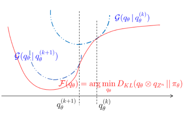
Figure 2: Mean-field Wasserstein gradient flow (MF-WGF) as an extension of the Majorize-Minimization (MM) algorithm [42] for minimizing (profile-KL) functional ℱ=minqZnDK​L(qθ⊗qZn∥πn)\mathcal{F}=\min_{q_{Z^{n}}}D_{KL}\big(q_{\theta}\otimes q_{Z^{n}}\,\big\|\,\pi_{n}\big) over the space of all probability measures on parameter space Θ\Theta. Here, 𝒢⁡(qθ|qθ′):=Vn​(qθ|qθ′)+12​τ​W22​(qθ,qθ′)\mathcal{G}(q_{\theta}\,|\,q_{\theta}^{\prime}):\,=V_{n}(q_{\theta}\,|\,q_{\theta}^{\prime})+\frac{1}{2\tau}W_{2}^{2}(q_{\theta},\,q_{\theta}^{\prime}) majorizes ℱ\mathcal{F}.

The perspective of viewing the parameter update step as minimizing a time-dependent KL divergence functional over 𝒫2​(Θ)\mathscr{P}_{2}(\Theta) leads to our new computational framework of MF-WGF for Bayesian latent variable models. More precisely, MF-WGF involves iteratively cycling through the following two steps for iteration k=0,1,…k=0,1,\ldots:

Step 1 (Local latent variable): For i=1,…,ni=1,\ldots,n, compute qZi(k+1)q^{(k+1)}_{Z_{i}} based on the updating formula (18);

Step 2 (Global model parameter): Compute the energy functional Vn​(qθ|qθ(k))V_{n}(q_{\theta}\,|\,q_{\theta}^{(k)}) using the most recent qZn(k+1)=⨂i=1nqZi(k+1)q^{(k+1)}_{Z^{n}}=\bigotimes_{i=1}^{n}q^{(k+1)}_{Z_{i}}, and update qθq_{\theta} via the one-step minimization movement scheme (2) with objective functional Vn​(qθ|qθ(k))V_{n}(q_{\theta}\,|\,q_{\theta}^{(k)}),

qθ(k+1)=argminqθVn​(qθ|qθ(k))+12​τ​W22​(qθ,qθ(k)).q_{\theta}^{(k+1)}=\mathop{\rm argmin~}_{q_{\theta}}V_{n}(q_{\theta}\,|\,q_{\theta}^{(k)})+\frac{1}{2\tau}W_{2}^{2}(q_{\theta},\,q_{\theta}^{(k)}). (19)

The two steps of MF-WGF resemble a distributional version of the E-step and the M-step respectively in the classical EM algorithm for dealing with missing data problems. One can also view MF-WGF as an Majorize-Minimization (MM) algorithm [42] for distributional optimization (see Figure 2 for an illustration) where 𝒢⁡(qθ|qθ′):=Vn​(qθ|qθ′)+12​τ​W22​(qθ,qθ′)\mathcal{G}(q_{\theta}\,|\,q_{\theta}^{\prime}):\,=V_{n}(q_{\theta}\,|\,q_{\theta}^{\prime})+\frac{1}{2\tau}W_{2}^{2}(q_{\theta},\,q_{\theta}^{\prime}) serves as the majorized version of the (profile) objective functional qθ↦minqZnDK​L(qθ⊗qZn∥πn)q_{\theta}\mapsto\min_{q_{Z^{n}}}D_{KL}\big(q_{\theta}\otimes q_{Z^{n}}\,\big\|\,\pi_{n}\big), where qZnq_{Z^{n}} has been profiled out since the minimizing over qZnq_{Z^{n}} admits a closed form solution as in Step 1 of MF-WGF.

Similar to Bayesian models without latent variables, in Section 4 we show that the MF solution (q^θ,q^Zn)(\widehat{q}_{\theta},\,\widehat{q}_{Z^{n}}) in (12) is a unique fixed point of the corresponding iterative procedure in a constant radius W2W_{2}-neighhorhood around the solution, and the iterative procedure has exponential convergence to this solution given it is initialized in this neighborhood. It is straightforward to show that q^θ\widehat{q}_{\theta}, as a fixed point to MF-WGF, satisfies

μ⁡(θ)=1Zn​(μ)​πθ​(θ)​e−n​Un​(θ,μ),with ​Zn​(μ)=∫Θπθ​(θ)​e−n​Un​(θ,μ)​𝑑θ,\displaystyle\mu(\theta)=\frac{1}{Z_{n}(\mu)}\,\pi_{\theta}(\theta)\,e^{-n\,U_{n}(\theta;\,\mu)},\quad\mbox{with }Z_{n}(\mu)=\int_{\Theta}\pi_{\theta}(\theta)\,e^{-n\,U_{n}(\theta;\,\mu)}\,{\rm d}\theta, (20)

which can be proved by applying the first order optimality condition to (19) in terms of the first variation (see Appendix D.1 for further details). This fixed point equation is helpful to show the concentration of MF approximation q^θ\widehat{q}_{\theta} towards the true parameter θ∗\theta^{\ast} (c.f. Theorem 4.2, also see Section 4.1 for a sketched proof). Heuristically, when nn is large, q^θ\widehat{q}_{\theta} is expected to concentrate around the point mass measure δθ∗\delta_{\theta^{\ast}} at θ∗\theta^{\ast}, so that we can roughly approximate q^θ\widehat{q}_{\theta} by the right hand side of (20) with μ\mu being replaced by δθ∗\delta_{\theta^{\ast}}; then the convergence follows by the fact that θ∗\theta^{\ast} approximately minimizes the potential Un​(θ,δθ∗)U_{n}(\theta;\,\delta_{\theta^{\ast}}).

4 Theoretical Results

In this subsection, we present two main theoretical results of this work: concentration of the MF approximation q^θ\widehat{q}_{\theta} to the true parameter θ∗\theta^{\ast}, and the convergence of the proposed MF-WGF algorithm. In the next section, we will apply the theoretical results to three representative examples by verifying the assumptions. All proofs are deferred to the Appendices in the supplement of the paper.

4.1 Analysis of mean-field approximation

We adopt the frequentist perspective by assuming that data XnX^{n} are generated from a data generating model indexed by a true parameter θ∗\theta^{\ast}. Before presenting the formal result, we make the following assumptions, most are standard for proving concentration of Bayesian posteriors [30, 64] and their MF counterpart [56, 80, 1, 82].

Assumption A.1 (test condition).

For some constants c1,c2>0c_{1},c_{2}>0 and any ε>c1​log⁡n/n\varepsilon>c_{1}\sqrt{\log n/n}, there is a test function ϕn\phi_{n}, such that

𝔼θ∗[ϕn]≤e−c2​n​ε2,supθ:∃j∈[m],s.t.‖θj−θj∗‖>ε𝔼θ[1−ϕn]≤e−c2​n​ε2.\displaystyle\mathbb{E}_{\theta^{\ast}}[\phi_{n}]\leq e^{-c_{2}n\varepsilon^{2}},\quad\sup_{\theta:\exists j\in[m],s.t.\|\theta_{j}-\theta_{j}^{\ast}\|>\varepsilon}\mathbb{E}_{\theta}[1-\phi_{n}]\leq e^{-c_{2}n\varepsilon^{2}}.

In a typical parametric setting, the existence of such a test can be proved by decomposing {θj:‖θj−θj∗‖>ε}\{\theta_{j}:\|\theta_{j}-\theta_{j}^{\ast}\|>\varepsilon\} into a countable union of annuluses. Each annuluses can be covered by a finite number of balls, within each ball the likelihood ratio type test can be employed [9, 43]. When m=1m=1 in Bayesian latent variable models, this is just the standard test condition discussed in [30, Section 7].

Assumption A.2 (prior thickness).

There is a measure Q~=⊗j=1mQ~j\widetilde{Q}=\otimes_{j=1}^{m}\widetilde{Q}_{j}, subsets Θ~j⊂Θj\widetilde{\Theta}_{j}\subset\Theta_{j} for j∈[m]j\in[m], and positive constants c3c_{3} and c4c_{4}, such that for any θ∈Θ~≔⊗j=1mΘ~j\theta\in\widetilde{\Theta}\coloneqq\otimes_{j=1}^{m}\widetilde{\Theta}_{j} we have

DKL(p(⋅|θ∗)∥p(⋅|θ))≤c4εn2,∫𝒳(logp⁡(x|θ∗)p⁡(x|θ))2p(x|θ∗)dx≤c4εn2,\displaystyle\,D_{\rm KL}\big(p(\cdot\,|\,\theta^{\ast})\,\|\,p(\cdot\,|\,\theta)\big)\leq c_{4}\varepsilon_{n}^{2},\quad\int_{\mathcal{X}}\Big(\log\frac{p(x\,|\,\theta^{\ast})}{p(x\,|\,\theta)}\Big)^{2}p(x\,|\,\theta^{\ast})\,{\rm d}x\leq c_{4}\varepsilon_{n}^{2},
log⁡d​Q~d​Πθ≤c4​n​εn2andlog⁡Q~​(Θ~)=∑j=1mlog⁡Q~j​(Θ~j)≥−c3​n​εn2,\displaystyle\,\log\frac{{\rm d}\widetilde{Q}}{{\rm d}\Pi_{\theta}}\leq c_{4}n\varepsilon_{n}^{2}\quad\mbox{and}\quad\log\widetilde{Q}(\widetilde{\Theta})=\sum_{j=1}^{m}\log\widetilde{Q}_{j}(\widetilde{\Theta}_{j})\geq-c_{3}n\varepsilon_{n}^{2},

where Πθ\Pi_{\theta} denotes the prior distribution, and εn=M​log⁡n/n\varepsilon_{n}=M\sqrt{\log n/n} for some M>1M>1.

The case of m=1m=1 reduces to the Bayesian posterior without MF approximation. Under m=1m=1, this assumption is implied by the standard prior thickness assumption [30] by taking Q~=Πθ\widetilde{Q}=\Pi_{\theta}. When m>1m>1, this assumption requires the existence of a fully factorized probability measure Q~\widetilde{Q} in the MF family that is close to the prior distribution and puts enough mass around the ground truth θ∗\theta^{\ast}.

For Bayesian latent variable models, we need an additional assumption on the conditional likelihood function of latent variable ZZ given θ\theta and observation XX.

Assumption A.3 (local bound of KL divergence).

The marginal distribution p⁡(x|θ)p(x\,|\,\theta) of observation XX under θ\theta and the conditional distribution p⁡(z|x,θ)p(z\,|\,x,\theta) of latent variable ZZ given X=xX=x and θ\theta satisfy

DK​L(p(⋅|x,θ∗)∥p(⋅|x,θ))\displaystyle D_{KL}\big(p(\cdot\,|\,x,\theta^{\ast})\,\|\,p(\cdot\,|\,x,\theta)\big) ≤G⁡(x)​εn2,∀θ∈Θ~,\displaystyle\leq G(x)\,\varepsilon_{n}^{2},\quad\forall\,\theta\in\widetilde{\Theta}, (21)

where Θ~\widetilde{\Theta} is the local neighborhood of θ∗\theta^{\ast} defined in Assumption A.2, and G⁡(X)G(X) is a sub-exponential random variable with parameters σ4\sigma_{4} under p(⋅|θ∗)p(\cdot\,|\,\theta^{\ast}), i.e. 𝔼θ∗​[exp⁡{σ4−1​|G⁡(X)|}]≤2\mathbb{E}_{\theta^{\ast}}\big[\exp\big\{\sigma_{4}^{-1}|G(X)|\big\}\big]\leq 2.

This assumption is a mild condition, which is implied by a quadratic growth of KL divergence for θ∈Θ~\theta\in\widetilde{\Theta}, i.e. DKL(p(⋅|x,θ∗)∥p(x,θ))≲G(X)∥θ−θ∗∥2D_{\rm KL}(p(\cdot\,|\,x,\theta^{\ast})\,\|\,p(x,\theta))\lesssim G(X)\|\theta-\theta^{\ast}\|^{2}. This quadratic growth property holds if the logarithms of both distributions (density or mass function) are twice differentiable with controlled Hessians. For simple presentation, we adopt the assumption that G⁡(X)G(X) is sub-exponential to derive a high probability upper bound of n−1​∑i=1nG⁡(Xi)n^{-1}\sum_{i=1}^{n}G(X_{i}). This sub-exponential assumption on G⁡(X)G(X) can be generalized to G⁡(X)G(X) having a finite Orlicz-norm. See Appendix G for the definition of the Orlicz norm of a random variable and further details.

Bayesian models without latent variables. Recall that q^θ\widehat{q}_{\theta} is the solution of the mean-field optimization problem (11), which should satisfy the following optimality condition (see Lemma C.1 in Appendix C.1),

q^j​(θj)=exp⁡{∫Θ−jlog⁡πθ​(θ)+∑k=1nlog⁡p⁡(Xk|θ)​d​q^−j​(θ−j)}∫Θjexp⁡{∫Θ−jlog⁡πθ​(θ)+∑k=1nlog⁡p⁡(Xk|θ)​d​q^−j​(θ−j)}​d​θj,for ​j∈[m].\displaystyle\widehat{q}_{j}(\theta_{j})=\frac{\exp\big\{\int_{\Theta_{-j}}\log\pi_{\theta}(\theta)+\sum_{k=1}^{n}\log p(X_{k}\,|\,\theta)\,{\rm d}\widehat{q}_{-j}(\theta_{-j})\big\}}{\int_{\Theta_{j}}\exp\big\{\int_{\Theta_{-j}}\log\pi_{\theta}(\theta)+\sum_{k=1}^{n}\log p(X_{k}\,|\,\theta)\,{\rm d}\widehat{q}_{-j}(\theta_{-j})\big\}\,{\rm d}\theta_{j}},\quad\mbox{for }j\in[m]. (22)

A major challenge in our analysis of the MF solution q^θ\widehat{q}_{\theta} is how to deal with the normalization constant (denominator) in the preceding display, which depends on q^θ\widehat{q}_{\theta} and complicates the analysis. To address this issue, we rewrite equation (22) by adding a θj\theta_{j}-independent term to both nominator and denominator,

q^j​(θj)=exp⁡{∫Θ−jlog⁡πθ​(θ)Q~j​(θj)​q^−j​(θ−j)+∑i=1nlog⁡p⁡(Xi|θ)p⁡(Xi|θ∗)​d​q^−j}​Q~j​(θj)∫Θjexp⁡{∫Θ−jlog⁡πθ​(θ)Q~j​(θj)​q^−j​(θ−j)+∑i=1nlog⁡p⁡(Xi|θ)p⁡(Xi|θ∗)​d​q^−j}​d​Q~j.\displaystyle\widehat{q}_{j}(\theta_{j})=\frac{\exp\big\{\int_{\Theta_{-j}}\log\frac{\pi_{\theta}(\theta)}{\widetilde{Q}_{j}(\theta_{j})\widehat{q}_{-j}(\theta_{-j})}+\sum_{i=1}^{n}\log\frac{p(X_{i}\,|\,\theta)}{p(X_{i}\,|\,\theta^{\ast})}\,{\rm d}\widehat{q}_{-j}\big\}\widetilde{Q}_{j}(\theta_{j})}{\int_{\Theta_{j}}\exp\big\{\int_{\Theta_{-j}}\log\frac{\pi_{\theta}(\theta)}{\widetilde{Q}_{j}(\theta_{j})\widehat{q}_{-j}(\theta_{-j})}+\sum_{i=1}^{n}\log\frac{p(X_{i}\,|\,\theta)}{p(X_{i}\,|\,\theta^{\ast})}\,{\rm d}\widehat{q}_{-j}\big\}\,{\rm d}\widetilde{Q}_{j}}.

To prove the concentration of q^j\widehat{q}_{j} around the parameter θj∗\theta_{j}^{\ast}, we can proceed as the usual steps for proving posterior concentration (e.g. [30, 64]) by proving an upper and a lower bound to the numerator and the denominator respectively. Applying a union bound then yields the concentration of q^θ\widehat{q}_{\theta} around θ∗\theta^{\ast} due to the factorization structure of q^θ\widehat{q}_{\theta}.

For the lower bound to the denominator in the preceding display, denoted as DjD_{j}, we utilize the following equivalent expression,

logDj=−W~n(q^θ)=−minqθ=⊗j=1mqjW~n(qθ),with\displaystyle\log D_{j}=-\widetilde{W}_{n}(\widehat{q}_{\theta})=-\min_{q_{\theta}=\otimes_{j=1}^{m}q_{j}}\widetilde{W}_{n}(q_{\theta}),\quad\mbox{with } (23)
W~n(qθ)=∫Θ\displaystyle\widetilde{W}_{n}(q_{\theta})=\int_{\Theta} ∑i=1nlogp⁡(Xi|θ∗)p⁡(Xi|θ)dq1(θ1)⋯dqm(θm)+DKL(q1⊗⋯⊗qm∥πθ).\displaystyle\sum_{i=1}^{n}\log\frac{p(X_{i}\,|\,\theta^{\ast})}{p(X_{i}\,|\,\theta)}\,{\rm d}q_{1}(\theta_{1})\cdots{\rm d}q_{m}(\theta_{m})+D_{\rm KL}(q_{1}\otimes\cdots\otimes q_{m}\,\|\,\pi_{\theta}).

Here, functional W~n\widetilde{W}_{n} is, up to a qθq_{\theta}-independent constant, the same as the objective functional qθ=⨂j=1mqj↦DK​L(qθ∥πn)q_{\theta}=\bigotimes_{j=1}^{m}q_{j}\mapsto D_{KL}\big(q_{\theta}\,\big\|\,\pi_{n}\big). Thus, q^θ\widehat{q}_{\theta} minimizes W~n\widetilde{W}_{n}. Since q^θ\widehat{q}_{\theta} is expected to be concentrated around θ∗\theta^{\ast}, we may use −W~n​(qθ)-\widetilde{W}_{n}(q_{\theta}) with some carefully constructed qθq_{\theta} (the Q~\widetilde{Q} from Assumption A.2) suitably concentrated around θ∗\theta^{\ast} (e.g. a uniform distribution supported on a small neighborhood around θ∗\theta^{\ast}) for providing a lower bound to log⁡Dj\log D_{j}.

For the upper bound to the numerator, the first term can be controlled by directly applying Jensen’s inequality; the second term ∑i=1nlog⁡p⁡(Xi|θ)p⁡(Xi|θ∗)\sum_{i=1}^{n}\log\frac{p(X_{i}\,|\,\theta)}{p(X_{i}\,|\,\theta^{\ast})}, which is roughly negative nn times DKL[p(⋅|θ∗)∥p(⋅|θ)]D_{\rm KL}\big[\,p(\cdot\,|\,\theta^{\ast})\,\big\|\,p(\cdot\,|\,\theta)\big] since {Xi}i=1n\{X_{i}\}_{i=1}^{n} are marginally i.i.d. from p(⋅|θ∗)p(\cdot\,|\,\theta^{\ast}) under the frequentist perspective. To formally bound the numerator, or more precisely, the integral of numerator over set Θε={∥θ−θ∗∥≥ε}\Theta_{\varepsilon}=\{\|\theta-\theta^{\ast}\|\geq\varepsilon\} for suitably large ε>0\varepsilon>0, we use the commonly adopted test condition (i.e., Assumption A.1) for uniformly controlling the log-likelihood ratio process over Θε\Theta_{\varepsilon}.

The following theorem shows the concentration of q^θ\widehat{q}_{\theta} by characterizing the tail probability of being away from the true parameter θ∗\theta^{\ast}. Recall that we are adopting a frequentist perspective, where the randomness in all high probability bound is coming from the randomness in the samples X1,⋯,XnX_{1},\cdots,X_{n} that are generated under a true parameter θ∗\theta^{\ast}.

Theorem 4.1 (Exponential posterior concentration without latent variables).

Under Assumptions A.1 and A.2, if the sample size satisfies c4​nc2​M2≥3​m​M2​log⁡nc_{4}n^{c_{2}M^{2}}\geq 3mM^{2}\log n, then for any M≥1M\geq 1, the MF variational approximation Q^θ\widehat{Q}_{\theta} to the posterior distribution of θ\theta satisfies the following with probability at least 1−2​c4n​εn2=1−2​c4M2​log⁡n1-\frac{2c_{4}}{n\varepsilon_{n}^{2}}=1-\frac{2c_{4}}{M^{2}\log n},

Q^θ(∃j∈[m]s.t.∥θj−θj∗∥>ε)≤e−c2nε2/2,\displaystyle\widehat{Q}_{\theta}\big(\exists\,j\in[m]\,\,s.t.\,\,\|\theta_{j}-\theta_{j}^{\ast}\|>\varepsilon\big)\leq e^{-c_{2}n\varepsilon^{2}/2},
for allε>M⁡(3+c1+2​c4+c3+1c2)​log⁡nn.\displaystyle\qquad\qquad\qquad\mbox{for all}\quad\varepsilon>M\Big(3+c_{1}+\frac{2c_{4}+c_{3}+1}{c_{2}}\Big)\sqrt{\frac{\log n}{n}}. (24)

Bayesian latent variable models. Let 𝒵={1,2,…,K}\mathcal{Z}=\{1,2,\ldots,K\} be the support of each discrete latent variable. In this case, q^θ\widehat{q}_{\theta} is the solution of the mean-field optimization problem (12), satisfying (see Lemma C.3 in Appendix C.2 and Appendix D.1),

q^θ​(θ)=1Z^n​πθ​(θ)​e−n​Un​(θ,q^θ),with ​Z^n=∫Θπθ​(θ)​e−n​Un​(θ,q^θ)​𝑑θ,\displaystyle\widehat{q}_{\theta}(\theta)=\frac{1}{\widehat{Z}_{n}}\,\pi_{\theta}(\theta)\,e^{-n\,U_{n}(\theta,\,\widehat{q}_{\theta})},\quad\mbox{with }\widehat{Z}_{n}=\int_{\Theta}\pi_{\theta}(\theta)\,e^{-n\,U_{n}(\theta,\,\widehat{q}_{\theta})}\,{\rm d}\theta, (25)

where the (sample) potential function Un:Θ×𝒫r​(Θ)→ℝU_{n}:\,\Theta\times\mathscr{P}^{r}(\Theta)\to\mathbb{R} is

Un​(θ,qθ)\displaystyle U_{n}(\theta,\,q_{\theta}) =−1n∑i=1n∑z=1Klogp(Xi,z|θ)Φ(qθ,Xi)(z),where\displaystyle=-\frac{1}{n}\sum_{i=1}^{n}\sum_{z=1}^{K}\log p(X_{i},z\,|\,\theta)\,\Phi(q_{\theta},X_{i})(z),\quad\mbox{where} (26)
Φ⁡(q^θCLOSE,\displaystyle\Phi(\widehat{q}_{\theta}, OPENXi)​(z):=q^Zi​(z)=exp⁡{𝔼q^θ​[log⁡p⁡(Xi,z|θ)]}∑k=1Kexp⁡{𝔼q^θ​[log⁡p⁡(Xi,k|θ)]},z∈[K].\displaystyle\,X_{i})(z):\,=\widehat{q}_{Z_{i}}(z)=\frac{\exp\big\{\mathbb{E}_{\widehat{q}_{\theta}}\big[\log p(X_{i},z\,|\,\theta)\big]\big\}}{\sum_{k=1}^{K}\exp\big\{\mathbb{E}_{\widehat{q}_{\theta}}\big[\log p(X_{i},k\,|\,\theta)\big]\big\}},\quad z\in[K].

Similar to the analysis of Bayesian models without latent variables, we rewrite equation (25) by adding a θ\theta-independent term to both nominator and denominator,

q^θ​(θ)=exp{−∑i=1n∑z=1KΦ(q^θ,Xi)(z)logΦ⁡(q^θ,Xi)​(z)p⁡(z|Xi,θ)−∑i=1nlogp⁡(Xi|θ∗)p⁡(Xi|θ)}πθ(θ)∫Θexp{−∑i=1n∑z=1KΦ(q^θ,Xi)(z)logΦ⁡(q^θ,Xi)​(z)p⁡(z|Xi,θ)−∑i=1nlogp⁡(Xi|θ∗)p⁡(Xi|θ)}dπθ(θ).\displaystyle\widehat{q}_{\theta}(\theta)=\frac{\exp\big\{-\sum_{i=1}^{n}\sum_{z=1}^{K}\Phi(\widehat{q}_{\theta},X_{i})(z)\log\frac{\Phi(\widehat{q}_{\theta},X_{i})(z)}{p(z\,|\,X_{i},\theta)}-\sum_{i=1}^{n}\log\frac{p(X_{i}\,|\,\theta^{\ast})}{p(X_{i}\,|\,\theta)}\big\}\,\pi_{\theta}(\theta)}{\int_{\Theta}\exp\big\{-\sum_{i=1}^{n}\sum_{z=1}^{K}\Phi(\widehat{q}_{\theta},X_{i})(z)\log\frac{\Phi(\widehat{q}_{\theta},X_{i})(z)}{p(z\,|\,X_{i},\theta)}-\sum_{i=1}^{n}\log\frac{p(X_{i}\,|\,\theta^{\ast})}{p(X_{i}\,|\,\theta)}\big\}\,{\rm d}\pi_{\theta}(\theta)}.

For the lower bound to the denominator, denoted as DnD_{n}, we can use the following equivalent expression, which is more convenient to analyze,

log⁡Dn=−Wn​(q^θ)=−minqθ⁡Wn​(qθ),with ​Wn​(qθ)=\displaystyle\log D_{n}=-W_{n}(\widehat{q}_{\theta})=-\min_{q_{\theta}}W_{n}(q_{\theta}),\quad\mbox{with }W_{n}(q_{\theta})= (27)
∫Θ{∑i=1n\displaystyle\int_{\Theta}\bigg\{\sum_{i=1}^{n} ∑z=1KΦ(qθ,Xi)(z)logΦ⁡(qθ,Xi)​(z)p⁡(Xi,z|θ)+∑i=1nlogp⁡(Xi|θ∗)p⁡(Xi|θ)}dqθ(θ)+DKL(qθ∥πθ).\displaystyle\,\sum_{z=1}^{K}\Phi(q_{\theta},X_{i})(z)\log\frac{\Phi(q_{\theta},X_{i})(z)}{p(X_{i},z\,|\,\theta)}+\sum_{i=1}^{n}\log\frac{p(X_{i}\,|\,\theta^{\ast})}{p(X_{i}\,|\,\theta)}\bigg\}\,{\rm d}q_{\theta}(\theta)+D_{\rm KL}(q_{\theta}\,\|\,\pi_{\theta}).

Here, functional WnW_{n} is, up to a qθq_{\theta}-independent constant, the same as the (profile) objective functional qθ↦minqZnDK​L(qθ⊗qZn∥πn)q_{\theta}\mapsto\min_{q_{Z^{n}}}D_{KL}\big(q_{\theta}\otimes q_{Z^{n}}\,\big\|\,\pi_{n}\big) after qZnq_{Z^{n}} being maxed out or replaced by Φ⁡(qθ,Xi)\Phi(q_{\theta},X_{i}); so q^θ\widehat{q}_{\theta} minimizes WnW_{n}. Again, we may use −Wn​(qθ)-W_{n}(q_{\theta}) with some carefully constructed qθq_{\theta} suitably concentrated around θ∗\theta^{\ast} (e.g. a uniform distribution supported on a small neighborhood around θ∗\theta^{\ast}) for providing a lower bound to log⁡Dn\log D_{n}.

For the upper bound to the numerator, the second term can be treated in the same way as in Bayesian models without latent variables. For the first term in the exponent, just note that

−∑z=1KΦ(q^θ,Xi)(z)logΦ⁡(q^θ,Xi)​(z)p⁡(z|Xi,θ)-\sum_{z=1}^{K}\Phi(\widehat{q}_{\theta},X_{i})(z)\log\frac{\Phi(\widehat{q}_{\theta},X_{i})(z)}{p(z\,|\,X_{i},\theta)}

is the negative KL divergence between two discrete measures, and therefore is non-positive.

The following theorem shows the concentration of q^θ\widehat{q}_{\theta} by characterizing the tail probability of being away from the true parameter θ∗\theta^{\ast} in Bayesian latent variable models.

Theorem 4.2 (Exponential posterior concentration with latent variables).

Under Assumptions A.1, A.2, and A.3, if the sample size satisfies 6​M​log⁡n≤min⁡{nc2​M,e4​n​σ4−1}6M\log n\leq\min\{n^{c_{2}M},e^{4n\sigma_{4}^{-1}}\}, then for any M≥1M\geq 1, the MF variational approximation Q^θ\widehat{Q}_{\theta} to the marginal posterior of θ\theta satisfies the following with probability at least 1−2​c4n​εn2=1−2​c4M2​log⁡n1-\frac{2c_{4}}{n\varepsilon_{n}^{2}}=1-\frac{2c_{4}}{M^{2}\log n},

Q^θ(∥θ−θ∗∥>ε)≤e−c2nε2/2,\displaystyle\widehat{Q}_{\theta}\big(\|\theta-\theta^{\ast}\|>\varepsilon\big)\leq e^{-{c_{2}n\varepsilon^{2}}/2}, (28)
for allε≥M⁡(3+c1+𝔼⁡[G⁡(X)]+c3+c4+2c2)​log⁡nn.\displaystyle\qquad\qquad\mbox{for all}\quad\varepsilon\geq M\Big(3+c_{1}+\frac{\mathbb{E}[G(X)]+c_{3}+c_{4}+2}{c_{2}}\Big)\,\sqrt{\frac{\log n}{n}}. (29)

Concentration properties of variational inference have been studied in the recent literature under different criteria. [1] and [80] consider a variant of the usual variational inference, called the α\alpha-variational inference, obtained by raising the likelihood to a fractional power α∈(0,1]\alpha\in(0,1] to facilitate the theoretical analysis. They prove upper bounds for the variational Bayes risk, defined as the expected Rényi divergence with respect to their α\alpha-fractional variational posterior. When α\alpha is strictly small than one, they only need a prior concentration assumption (similar to our Assumption A.2); however, under some mild conditions their risk function behaves like the second moment 𝔼Q^θ​[‖θ−θ∗‖2]\mathbb{E}_{\widehat{Q}_{\theta}}\big[\|\theta-\theta^{\ast}\|^{2}\big], which is much weaker than our sub-Gaussian type tail result. For the usual variational inference (or α\alpha-variational inference with α=1\alpha=1), [56, 80, 82] proves high probability upper bounds to some similar variational Bayes risks that scales as 𝔼Q^θ​[‖θ−θ∗‖2]\mathbb{E}_{\widehat{Q}_{\theta}}\big[\|\theta-\theta^{\ast}\|^{2}\big] under similar test conditions (as our Assumption A.1) and a stronger version of the prior concentration assumption. Their proofs avoid assuming the compactness of parameter space by considering a sequence of sieve sets. [33] proves a similar sub-Gaussian concentration result as ours; their proof is based on a perturbation analysis specifically tailored to the MF approximation and does not seem easily generalizable to other variatioal or hybrid schemes.

Our proof technique is very different from existing proofs of the variational posterior concentration in the literature, most of which are based on applying the varitional characterization of KL divergence, DKL(p||q)=suph{∫hp−log(∫ehq)}D_{\rm KL}(p\,||\,q)=\sup_{h}\big\{\int hp-\log(\int e^{h}q)\big\}. We instead view the variational posterior Q^θ\widehat{Q}_{\theta} as a point in the Wasserstein space 𝕎2​(ℝd)\mathbb{W}_{2}(\mathbb{R}^{d}) that minimizes a KL divergence functional, and uses its first order optimality condition (or equivalently, its stationarity to the time-discrete WGF) to show the concentration via subdiffential calculus in 𝕎2​(ℝd)\mathbb{W}_{2}(\mathbb{R}^{d}). This general perspective might be useful in extending the developed proof technique to other approximation scheme beyond MF, such as many recent generative model based variational inference procedures. Our obtained rate of convergence is also nearly optimal in the parametric setting; and the assumptions we made needed are standard in Bayesian asymptotics literature, and appears to be among the weakest in the context of variational inference. In addition, our proof techniques can be straightforwardly extended to non-parametric settings where the optimal rate of convergence is slower than root-nn.

4.2 Analysis of MF-WGF algorithm

We separately analyze the convergence of MF-WGF for Bayesian models with/without latent variables.

Bayesian models without latent variables. Recall that in the kk-th iteration, the MF-WGF algorithm updates the joint variational distribution ⨂j=1mqj(k)\bigotimes_{j=1}^{m}q_{j}^{(k)} into ⨂j=1mqj(k+1)\bigotimes_{j=1}^{m}q_{j}^{(k+1)} with

qj(k+1)=argminqjn𝔼qj⊗q−j(k)[Un]+DKL(qj⊗q−j(k)∥πθ)+12​τW22(qj,qj(k)),j∈[m],\displaystyle q_{j}^{(k+1)}=\mathop{\rm argmin~}_{q_{j}}n\,\mathbb{E}_{q_{j}\otimes q_{-j}^{(k)}}\big[U_{n}\big]+D_{\rm KL}\big(q_{j}\otimes q_{-j}^{(k)}\,\big\|\,\pi_{\theta}\big)+\frac{1}{2\tau}W_{2}^{2}(q_{j},q_{j}^{(k)}),\quad j\in[m],

where Un(θ)=−1n∑i=1nlogp(Xi|θ)U_{n}(\theta)=-\frac{1}{n}\sum_{i=1}^{n}\log p(X_{i}\,|\,\theta) is the sample potential function. The corresponding population-level potential function is

U(θ)=−∫ℝdlogp(x|θ)p(dx|θ∗).\displaystyle U(\theta)=-\int_{\mathbb{R}^{d}}\log p(x\,|\,\theta)\,p({\rm d}x\,|\,\theta^{\ast}).

We expect that UnU_{n} and UU are uniformly close enough when the sample size nn is sufficiently large (e.g. Theorem 1 in [49]).

Before formally presenting our result, we begin by introducing several assumptions that are commonly used to prove exponential convergence of iterative algorithms in optimization literature.

Assumption B.1 (strong convexity of population-level potential).

There exists λ>0\lambda>0 such that UU is λ\lambda-strongly convex, i.e.

U⁡((1−t)​θ+t​θ′)≤(1−t)​U​(θ)+t​U​(θ′)−λ2​t​(1−t)​‖θ−θ′‖2\displaystyle U\big((1-t)\theta+t\theta^{\prime}\big)\leq(1-t)\,U(\theta)+t\,U(\theta^{\prime})-\frac{\lambda}{2}\,t(1-t)\|\theta-\theta^{\prime}\|^{2}

for all t∈[0,1]t\in[0,1] and θ,θ′∈Θ\theta,\theta^{\prime}\in\Theta. Moreover, the parameter space Θ=⨂j=1mΘj⊂ℝd\Theta=\bigotimes_{j=1}^{m}\Theta_{j}\subset\mathbb{R}^{d} is convex and contained a ball centered at the origin with radius RR.

This strong convexity assumption guarantees that DKL(⋅∥πn)D_{\rm KL}(\cdot\,\|\,\pi_{n}) is strongly convex along generalized geodesics on 𝒫2r(Θ1)×⋯×𝒫2r(Θm)⊂𝒫2r(Θ)\mathscr{P}_{2}^{r}(\Theta_{1})\times\cdots\times\mathscr{P}_{2}^{r}(\Theta_{m})\subset\mathscr{P}_{2}^{r}(\Theta). It is possible to relax this global strong convexity to a local strong convexity within a small but constant-radius neighborhood around the true parameter θ∗\theta^{\ast}, which is always true for regular models with non-singular Fisher information matrix. One simple strategy is to assume that both the prior and the initialization distribution of the algorithm are supported within this neighborhood. In practice, one can construct this initialization distribution by identifying a reasonably good initial point estimate of θ∗\theta^{\ast}, for example, using simple and fast methods such as the method of moments; and also modify the prior by restricting it onto a constant neighborhood around the estimate. Due to the flexibility in selecting the prior distribution for MF-WGF, such a modification will have a minimal impact on the implementation. A second technical strategy is to further impose a dissipative condition (see [58] for definition). A dissipative condition is commonly made to guarantee the long term stability of sampling algorithms such as Langevin dynamics [58] as it causes most probability mass absorbed into a constant neighborhood of θ∗\theta^{\ast} after a number of iterations; then the behavior of the algorithm inside this neighborhood is driven by the local convexity of the potential. Since Theorem 4.1 tells that there is at most O⁡(e−c​n)O\big(e^{-cn}\big) probability mass of q^θ\widehat{q}_{\theta} outside this neighborhood, we expect our current analysis to be valid up to an extra O⁡(e−c​n)O\big(e^{-cn}\big) remainder term. Due to the significant complexity of our current proof with global convexity, we will leave a systematic study on such an extension in a separate work.

Assumption B.2 (smoothness of population-level potential).

There exists L>0L>0 such that UU is LL-smooth, which is defined by

U⁡((1−t)​θ+t​θ′)≥(1−t)​U​(θ)+t​U​(θ′)−L2​t​(1−t)​‖θ−θ′‖2\displaystyle U\big((1-t)\theta+t\theta^{\prime}\big)\geq(1-t)\,U(\theta)+t\,U(\theta^{\prime})-\frac{L}{2}\,t(1-t)\|\theta-\theta^{\prime}\|^{2} (30)

for all t∈[0,1]t\in[0,1] and θ,θ′∈Θ\theta,\theta^{\prime}\in\Theta.

A smoothness condition on the objective function is usually necessary to prove exponential convergence of a coordinate descent-type optimization algorithms [77, 78]. When UU is twice differentiable, the above Assumption B.2 is equivalent to ‖|∇2U​(θ)|‖op≤L{\left|\kern-1.07639pt\left|\kern-1.07639pt\left|\nabla^{2}U(\theta)\right|\kern-1.07639pt\right|\kern-1.07639pt\right|}_{\rm op}\leq L for all θ∈Θ\theta\in\Theta. In our proof, we can slightly relax this condition since we only require ‖∇jU​(θj,θ−j)−∇jU​(θj,θ−j′)‖≤L​‖θ−j−θ−j′‖\|\nabla_{j}U(\theta_{j},\theta_{-j})-\nabla_{j}U(\theta_{j},\theta_{-j}^{\prime})\|\leq L\|\theta_{-j}-\theta_{-j}^{\prime}\|, where ∇j\nabla_{j} is the gradient with respect to the jjth component of UU. This inequality is equivalent to ‖|∇j∇−j​U​(θ)|‖op≤L{\left|\kern-1.07639pt\left|\kern-1.07639pt\left|\nabla_{j}\nabla_{-j}U(\theta)\right|\kern-1.07639pt\right|\kern-1.07639pt\right|}_{\rm op}\leq L when UU is twice differentiable and is weaker than Assumption B.2.

To show that the sample-level potential UnU_{n} is uniformly close to its population version UU and inherits the convexity and the smoothness of UU (see the proof of Theorem 4.3 in Appendix C.3), we need the following assumption which characterizes the continuity and the sub-exponential tail of the (higher-order) derivatives of the log-likelihood functions.

Assumption B.3 (regularity of log-likelihood function).

The log-likelihood function log⁡p⁡(x|θ)\log p(x\,|\,\theta) is twice differentiable with respect to θ∈Θ\theta\in\Theta. Let XX denote a sample generated from the true distribution p(⋅|θ∗)p(\cdot\,|\,\theta^{\ast}). Then, the following regularity assumptions hold.

  1. 1.

    The Lipschitz constant (relative to the matrix operator norm) of the log-likelihood Hessian

    J⁡(X):=supθ≠θ′‖|∇2​log​p​(X|θ)−∇2​log​p​(X|θ′)|‖op‖θ−θ′‖\displaystyle J(X):=\sup_{\theta\neq\theta^{\prime}}\frac{{\left|\kern-1.07639pt\left|\kern-1.07639pt\left|\nabla^{2}\log p(X\,|\,\theta)-\nabla^{2}\log p(X\,|\,\theta^{\prime})\right|\kern-1.07639pt\right|\kern-1.07639pt\right|}_{\rm op}}{\|\theta-\theta^{\prime}\|}

    satisfies 𝔼θ∗​[J⁡(X)]<J∗\mathbb{E}_{\theta^{\ast}}[J(X)]<J_{\ast} for some finite J∗J_{\ast}.

  2. 2.

    For any v∈Bℝd​(0,1)v\in B_{\mathbb{R}^{d}}(0,1) and θ∈Θ\theta\in\Theta, ⟨v,∇2​log​p​(X|θ)​v⟩\big\langle v,\nabla^{2}\log p(X\,|\,\theta)v\big\rangle is sub-exponential with parameter σ5\sigma_{5}. In particular, a sufficient condition for this to be true is ‖|∇2​log​p​(X|θ)|‖op{\left|\kern-1.07639pt\left|\kern-1.07639pt\left|\nabla^{2}\log p(X\,|\,\theta)\right|\kern-1.07639pt\right|\kern-1.07639pt\right|}_{\rm op} being sub-exponential for any θ∈Θ\theta\in\Theta.

The first part of this assumption can be checked by controlling the third order derivatives of log⁡p⁡(X|θ)\log p(X\,|\,\theta) with respect to θ\theta when it is sufficiently smooth; the second part can be verified by directly calculating the first order Orlicz norm of vT​∇2​log⁡p⁡(X|θ)​vv^{T}\nabla^{2}\log p(X\,|\,\theta)\,v, and can also be extended to a bounded ψα\psi_{\alpha} (Orlicz) norm for some α>0\alpha>0.

Theorem 4.3 (MF-WGF without latent variables).

Suppose Assumptions B.1–B.3 hold, and log⁡πθ\log\pi_{\theta} is twice differentiable. Then there is a universal constant C>0C>0, such that for any fixed η∈(0,1)\eta\in(0,1), the following inequality holds with probability at least 1−η1-\eta,

W22​(q(k),q^)≤(1+2​τ​λl​b−Lu​b2​τ2​m)−k​W22​(q(0),q^),k≥1,\displaystyle W_{2}^{2}(q^{(k)},\widehat{q})\leq\big(1+2\tau\lambda_{lb}-L_{ub}^{2}\tau^{2}m\big)^{-k}W_{2}^{2}(q^{(0)},\widehat{q}),\quad k\geq 1,

when n≥C​d​log⁡d⋅max⁡{log⁡J∗/log⁡d,log⁡(R​σ5/η),1}n\geq Cd\log d\cdot\max\big\{\log J_{\ast}/\log d,\log(R\sigma_{5}/\eta),1\big\} and the step size τ\tau satisfies

τ−1≥m​Lu​b,and1+2​τ​λl​b−Lu​b2​τ2​m≥0,\displaystyle\tau^{-1}\geq\sqrt{m}L_{ub},\quad\mbox{and}\quad 1+2\tau\lambda_{lb}-L_{ub}^{2}\tau^{2}m\geq 0,

where

λl​b\displaystyle\lambda_{lb} ≔n​λ−λmax​(∇2​log​πθ)−σ52​C​d​log⁡nn⋅max⁡{log⁡J∗log⁡d,log⁡R​σ5η,1},\displaystyle\coloneqq n{\lambda}-\lambda_{\max}(\nabla^{2}\log\pi_{\theta})-\sigma_{5}^{2}\sqrt{\frac{Cd\log n}{n}\cdot\max\Big\{\frac{\log J_{\ast}}{\log d},\log\frac{R\sigma_{5}}{\eta},1\Big\}},
Lu​b\displaystyle L_{ub} ≔n​L−λmin​(∇2​log​πθ)+σ52​C​d​log⁡nn⋅max⁡{log⁡J∗log⁡d,log⁡R​σ5η,1},\displaystyle\coloneqq nL-\lambda_{\min}(\nabla^{2}\log\pi_{\theta})+\sigma_{5}^{2}\sqrt{\frac{Cd\log n}{n}\cdot\max\Big\{\frac{\log J_{\ast}}{\log d},\log\frac{R\sigma_{5}}{\eta},1\Big\}},

and λmax​(∇2​log​πθ)\lambda_{\max}(\nabla^{2}\log\pi_{\theta}) and λmin​(∇2​log​πθ)\lambda_{\min}(\nabla^{2}\log\pi_{\theta}) are the largest and the smallest eigenvalues of the Hessian matrix ∇2​log​πθ\nabla^{2}\log\pi_{\theta} in Θ\Theta respectively. In particular, if we take τ=λl​b/(Lu​b2​m)\tau=\lambda_{lb}/(L_{ub}^{2}m), then

W22​(q(k),q^)≤(1+λl​b2Lu​b2​m)−k​W22​(q(0),q^),k≥1.\displaystyle W_{2}^{2}(q^{(k)},\widehat{q})\leq\Big(1+\frac{\lambda_{lb}^{2}}{L_{ub}^{2}m}\Big)^{-k}W_{2}^{2}(q^{(0)},\widehat{q}),\quad k\geq 1. (31)

The proof of this theorem does not require utilizing the concentration property on q^θ\widehat{q}_{\theta} as stated in Theorem 4.1, and the exponential convergence is solely driven by the convexity of population level potential UU. However, when an effective potential UnU_{n} varies across iterations, which is the case in MF-WGF for Bayesian latent variable models, the concentration property becomes essential to manage the fluctuation of UnU_{n}.

Equation (31) implies that O⁡(m​Lu​b2λl​b2​log⁡(1ε))=O⁡(m​L2λ2​log⁡(1ε))O\big(\frac{mL_{ub}^{2}}{\lambda_{lb}^{2}}\log\big(\frac{1}{\varepsilon}\big)\big)=O\big(\frac{mL^{2}}{\lambda^{2}}\log\big(\frac{1}{\varepsilon}\big)\big) iterations are sufficient for the algorithm to achieve an accuracy of ε∈(0,1)\varepsilon\in(0,1) in computing q^\widehat{q}. This iteration complexity matches a typical iteration complexity of coordinate gradient descent for minimizing a strongly convex and smooth function in the Euclidean space when taking the step size in the order of O⁡(λL2​m)O\big(\frac{\lambda}{L^{2}m}\big) as we do (see, e.g., Theorem 6.3 of [78]). However, analyzing the coordinate proximal gradient descent in a product Wasserstein space presents some unique challenges.

In the Euclidean space, ‖(x(k+1)−x(k))−(x^−x(k))‖=‖x(k+1)−x^‖\|(x^{(k+1)}-x^{(k)})-(\widehat{x}-x^{(k)})\|=\|x^{(k+1)}-\widehat{x}\| holds for any arbitrary points x^\widehat{x}, x(k)x^{(k)}, and x(k+1)x^{(k+1)}. However, we only have ‖Tqj(k)qj(k+1)−Tqj(k)q^j‖L2​(qj(k),Θj)2≥W22​(qj(k+1),q^j)\big\|T_{q_{j}^{(k)}}^{q_{j}^{(k+1)}}-T_{q_{j}^{(k)}}^{\widehat{q}_{j}}\big\|^{2}_{L^{2}(q_{j}^{(k)};\Theta_{j})}\geq W_{2}^{2}(q_{j}^{(k+1)},\widehat{q}_{j}) due to the positive curvature of the Wasserstein space. This difference indicates that we have to evaluate the change of KL divergence along the generalized geodesics (see Appendix A.4 for a definition) connecting qj(k+1)q_{j}^{(k+1)} and q^j\widehat{q}_{j} with the base measure qj(k)q_{j}^{(k)}, rather than the geodesics connecting qj(k+1)q_{j}^{(k+1)} and q^j\widehat{q}_{j}.

In the proof, the convexity of the potential function U⁡(θ)U(\theta) plays two roles: (1) allowing us to apply Theorem A.4 to control the subdifferential; (2) deriving a quadratic growth property of the KL-divergence functional, i.e.

DKL(q1⊗⋯⊗qm∥πn)−DKL(q^1⊗⋯⊗q^m∥πn)≳W22(q,q^θ),∀qj∈𝒫2r(Θj),j∈[m].D_{\rm KL}(q_{1}\otimes\cdots\otimes q_{m}\,\|\,\pi_{n})-D_{\rm KL}(\widehat{q}_{1}\otimes\cdots\otimes\widehat{q}_{m}\,\|\,\pi_{n})\gtrsim W_{2}^{2}(q,\widehat{q}_{\theta}),\quad\forall\,q_{j}\in\mathscr{P}_{2}^{r}(\Theta_{j}),\,\,j\in[m].

LL-smoothness of U⁡(θ)U(\theta) helps guarantee that the KL divergence between q(k)q^{(k)} and πn\pi_{n} is decreasing when the step size is small. The detailed proof is postponed to Appendix C.3.

Bayesian latent variable models. Recall that with the presence of latent variables, the MF-WGF algorithm can be summarized by the following iterative updating rule: for k=0,1,…k=0,1,\ldots,

qθ(k+1)=argminqθVn​(qθ|qθ(k))+12​τ​W22​(qθ,qθ(k)),q_{\theta}^{(k+1)}=\mathop{\rm argmin~}_{q_{\theta}}V_{n}(q_{\theta}\,|\,q_{\theta}^{(k)})+\frac{1}{2\tau}W_{2}^{2}(q_{\theta},\,q_{\theta}^{(k)}),

where for any qθ′∈𝒫⁡(θ)q_{\theta}^{\prime}\in\mathscr{P}(\theta), the (sample) energy (or KL divergence) functional Vn(⋅|qθ′)V_{n}(\cdot\,|\,q_{\theta}^{\prime}) is defined as

Vn(qθ|qθ′):=n𝔼qθ[Un(θ;qθ′)]+DKL(qθ||πθ),\displaystyle V_{n}(q_{\theta}\,|\,q_{\theta}^{\prime}):\,=n\,\mathbb{E}_{q_{\theta}}\big[U_{n}(\theta;\,q^{\prime}_{\theta})\big]+D_{\rm KL}(q_{\theta}\,||\,\pi_{\theta}),

and Un​(⋅,qθ′)U_{n}(\cdot\,;\,q^{\prime}_{\theta}) is the (sample) potential function given in (26). The corresponding population version of the potential is

U(θ;qθ′)=−∫ℝd{∑z=1Klogp(x,z|θ)Φ(qθ′,x)(z)}p(dx|θ∗).U(\theta;\,q_{\theta}^{\prime})=-\int_{\mathbb{R}^{d}}\bigg\{\sum_{z=1}^{K}\log p(x,z\,|\,\theta)\,\Phi(q_{\theta}^{\prime},x)(z)\bigg\}\,p({\rm d}x\,|\,\theta^{\ast}). (32)

The main difficulty in analyzing this MF-WGF algorithm is that the energy functional Vn(⋅|qθ(k))V_{n}(\,\cdot\,|\,q_{\theta}^{(k)}) determining qθ(k+1)q_{\theta}^{(k+1)} also depends on the previous iterate qθ(k)q_{\theta}^{(k)}. With a time-independent energy functional, whose global minimizer denoted as π∗\pi^{\ast}, we may directly apply Theorem 2.1 with π=π∗\pi=\pi^{\ast} to prove the contraction of the one-step discrete WGF towards π∗\pi^{\ast}. However, by directly applying Theorem 2.1 with π\pi therein being the minimizer of Vn(⋅|qθ(k))V_{n}(\,\cdot\,|\,q_{\theta}^{(k)}), we can only prove the one-step contraction of MF-WGF towards this minimizer, which changes over iteration count kk and is generally different from the target q^θ\widehat{q}_{\theta}.

To overcome this difficulty in the convergence analysis, we may introduce an accompanied population-level MF-WGF, defined as

q~θ(k+1)=argminqθV⁡(qθ|δθ∗)+12​τ​W22​(qθ,q~θ(k)),\displaystyle\widetilde{q}_{\theta}^{(k+1)}=\mathop{\rm argmin~}_{q_{\theta}}V(q_{\theta}\,|\,\delta_{\theta^{\ast}})+\frac{1}{2\tau}W_{2}^{2}(q_{\theta},\,\widetilde{q}_{\theta}^{(k)}), (33)

obtained by replacing qθ(k)q_{\theta}^{(k)} in Vn(⋅|qθ(k))V_{n}(\cdot\,|\,q_{\theta}^{(k)}) by the point mass measure δθ∗\delta_{\theta^{\ast}} at θ∗\theta^{\ast}, and the sample energy functional by its population counterpart

V(qθ|qθ′):=n𝔼qθ[U(θ;qθ′)]+DKL(qθ||πθ).\displaystyle V(q_{\theta}\,|\,q_{\theta}^{\prime}):\,=n\,\mathbb{E}_{q_{\theta}}\big[U(\theta;\,q^{\prime}_{\theta})\big]+D_{\rm KL}(q_{\theta}\,||\,\pi_{\theta}). (34)

Since the energy function V(⋅|δθ∗)V(\cdot\,|\,\delta_{\theta^{\ast}}) in the population-level MF-WGF is time-independent, we can apply Theorem 2.1 or Corollary 2.2 to prove its contraction. Moreover, since q^θ\widehat{q}_{\theta} is expected to be concentrated around θ∗\theta^{\ast}, we may expect the trajectory of the sample-level MF-WGF to be close to that of the population-level MF-WGF under the same initialization.

Based on this discussion, a natural strategy to prove the convergence of the MF-WGF algorithm can be divided into two main steps: 1. control the difference between the sample-level iterates {qθ(k):k≥0}\big\{q_{\theta}^{(k)}:\,k\geq 0\big\} and the population-level iterates {q~θ(k):k≥0}\big\{\widetilde{q}_{\theta}^{(k)}:\,k\geq 0\big\}; 2. analyze the convergence of population-level MF-WGF (33). Our actual proof is slightly different from the above heuristics. Specifically, to simplify the proof, we do not explicitly bound the difference between the sample-level and population-level iterates, but use some population level quantities, such as potential UU and energy functional VV, to substitute their sample versions and properly control the resulting extra error terms in analyzing the sample iterates (see Appendix C.4 for further details). In particular, the freedom of choosing an arbitrary π\pi in Theorem 2.1 allows us to directly apply the theorem to analyze the sample-level MF-WGF by taking π=q^θ\pi=\widehat{q}_{\theta}; however, some careful perturbation analysis will be required for the proof to go through.

The following assumptions are needed to formally prove the convergence of MF-WGF.

Assumption C.1 (strong convexity of population-level potential).

There exists some constant r>0r>0, such that for any μ∈B𝕎2​(δθ∗,r):={μ∈𝒫2r​(ℝd):W2​(μ,δθ∗)≤r}\mu\in B_{\mathbb{W}_{2}}(\delta_{\theta^{\ast}},r):\,=\big\{\mu\in\mathscr{P}_{2}^{r}(\mathbb{R}^{d}):\,W_{2}(\mu,\,\delta_{\theta^{\ast}})\leq r\big\}, function U⁡(⋅,μ):Θ→ℝU(\cdot\,;\,\mu):\Theta\to\mathbb{R} is λ\lambda-strongly convex, i.e.

U⁡((1−t)​θ+t​θ′,μ)≤(1−t)​U​(θ,μ)+t​U​(θ′,μ)−λ2​t​(1−t)​‖θ−θ′‖2U\big(\,(1-t)\,\theta+t\,\theta^{\prime}\,;\,\mu\big)\leq(1-t)\,U(\theta,\mu)+t\,U(\theta^{\prime},\mu)-\frac{\lambda}{2}\,t(1-t)\,\|\theta-\theta^{\prime}\|^{2} (35)

for all t∈[0,1]t\in[0,1] and θ,θ′∈Θ\theta,\theta^{\prime}\in\Theta. Moreover, parameter space Θ⊂ℝd\Theta\subset\mathbb{R}^{d} is convex and contained a ball centered at the origin with radius RR.

Notice that this assumption only requires U⁡(⋅,μ)U(\cdot\,;\,\mu) to be strongly convex when μ\mu is close to δθ∗\delta_{\theta^{\ast}}. We will verify this assumption for the two applications considered in Section 6. When the initialization qθ(0)q_{\theta}^{(0)} is close enough to the δθ∗\delta_{\theta^{\ast}}, it can be proved by induction that any later iterates qθ(k)q^{(k)}_{\theta} will stay in the same W2W_{2} neighborhood. Therefore, we do not need U⁡(⋅,μ)U(\cdot\,;\,\mu) to be strongly convex for all μ∈𝒫2r​(Θ)\mu\in\mathscr{P}_{2}^{r}(\Theta). This assumption plays a similar role as Assumption B.1 for models without latent variable. Similarly, we expect that the strong convexity of U⁡(θ,μ)U(\theta\,;\,\mu) with respect to parameter θ\theta can be relaxed to a local strong convexity within a neighborhood of θ∗\theta^{\ast} with sufficiently small constant radius for all μ∈B𝕎2​(0,r)\mu\in B_{\mathbb{W}_{2}}(0,r). Here, we simply assume the global strictly convexity of UU in the current analysis to avoid these technicalities without affecting the convey of our main proof ideas.

To show that the sample-level potential UnU_{n} is uniformly close to its population version UU and inherits the convexity property of UU (see Lemma C.6 in Appendix C.4), we need the following assumption characterizing continuity and sub-Gaussianity of the (higher-order) derivatives of the log-likelihood functions with the latent variable and the observed data.

Assumption C.2 (regularity of log-likelihood function).

The log-conditional-likelihood function log⁡p⁡(z|x,θ)\log p(z\,|\,x,\theta) of the latent variable ZZ and the log-marginal-likelihood function log⁡p⁡(x|θ)\log p(x\,|\,\theta) of the observation XX are twice differentiable with respect to θ\theta for all z∈[K]z\in[K] and x∈ℝdx\in\mathbb{R}^{d}. Let XX denote a sample from the true underlying data generating distribution p(⋅|θ∗)p\,(\,\cdot\,|\,\theta^{\ast}), then the following properties hold.

  1. 1.

    For i=1,2i=1,2, the random variable Si​(X):=∑k=1K‖∇log⁡p​(k|X,θ∗)‖2iS_{i}(X):=\sum_{k=1}^{K}\big\|\nabla\log p(k\,|\,X,\theta^{\ast})\big\|_{2}^{i} has finite expectation; and S2​(X)S_{2}(X) is sub-exponential with parameter σ3<∞\sigma_{3}<\infty, i.e. 𝔼​exp⁡{σ3−1​|S2​(X)|}≤2.\mathbb{E}\exp\{\sigma_{3}^{-1}|S_{2}(X)|\}\leq 2.

  2. 2.

    If we denote the Lipschitz constant of the log-likelihood Hessian by

    Jk​(X):=supθ≠θ′‖|∇2​log​p​(X,k|θ)−∇2​log​p​(X,k|θ′)|‖op‖θ−θ′‖,J_{k}(X):=\sup_{\theta\neq\theta^{\prime}}\frac{{\left|\kern-1.07639pt\left|\kern-1.07639pt\left|\nabla^{2}\log p(X,k\,|\,\theta)-\nabla^{2}\log p(X,k\,|\,\theta^{\prime})\right|\kern-1.07639pt\right|\kern-1.07639pt\right|}_{\rm op}}{\|\theta-\theta^{\prime}\|},

    then there exist some finite constant J∗J_{\ast} such that ∑k=1K𝔼θ∗​[Jk​(X)]≤J∗\sum_{k=1}^{K}\mathbb{E}_{\theta^{\ast}}[J_{k}(X)]\leq J_{\ast}.

  3. 3.

    For any v∈Bℝd​(0,1)v\in B_{\mathbb{R}^{d}}(0,1) and θ∈Θ\theta\in\Theta, ∑k=1Kp⁡(k|X,θ∗)⋅⟨v,∇2​log​p​(X,k|θ)​v⟩\sum_{k=1}^{K}p(k\,|\,X,\theta^{\ast})\cdot\big\langle v,\nabla^{2}\log p(X,k\,|\,\theta)\,v\big\rangle is sub-exponential with parameter σ1\sigma_{1}. In particular, a sufficient condition for this to hold is ‖|∇2​log​p​(X,k|θ)|‖op{\left|\kern-1.07639pt\left|\kern-1.07639pt\left|\nabla^{2}\log p(X,k\,|\,\theta)\right|\kern-1.07639pt\right|\kern-1.07639pt\right|}_{\rm op} being sub-exponential for any θ∈Θ\theta\in\Theta and k∈[K]k\in[K].

  4. 4.

    λ⁡(X):=supθ∈Θ,k∈[K]‖|∇2​log​p​(k|X,θ)|‖op\lambda(X):\,=\sup_{\theta\in\Theta,k\in[K]}{\left|\kern-1.07639pt\left|\kern-1.07639pt\left|\nabla^{2}\log p(k\,|\,X,\theta)\right|\kern-1.07639pt\right|\kern-1.07639pt\right|}_{\rm op} is sub-exponential with parameter σ2\sigma_{2}.

Parts 3 and 4 of the assumption can also be extended to a bounded ψα\psi_{\alpha} (Orlicz) norm for some α>0\alpha>0. Now we present our main theoretical result on the convergence of MF-WGF for Bayesian latent variable models.

Theorem 4.4 (MFVI with latent variables).

Suppose Assumptions A.1–A.3 and C.1–C.2 hold, and log⁡πθ\log\pi_{\theta} is twice differentiable. Let γ\gamma denote the operator norm of the missing data Fisher information matrix IS​(θ∗)I_{S}(\theta^{\ast}), i.e. γ=‖|IS​(θ∗)|‖op\gamma={\left|\kern-1.07639pt\left|\kern-1.07639pt\left|I_{S}(\theta^{\ast})\right|\kern-1.07639pt\right|\kern-1.07639pt\right|}_{\rm op} where

IS​(θ∗)=∫ℝd∑z=1Kp⁡(z|x,θ∗)​[∇log⁡p​(z|x,θ∗)]​[∇log⁡p​(z|x,θ∗)]T​p​(x|θ∗)​𝑑x,\displaystyle I_{S}(\theta^{\ast})=\int_{\mathbb{R}^{d}}\sum_{z=1}^{K}p(z\,|\,x,\theta^{\ast})\big[\nabla\log p(z\,|\,x,\theta^{\ast})\big]\big[\nabla\log p(z\,|\,x,\theta^{\ast})\big]^{T}p(x\,|\,\theta^{\ast})\,{\rm d}x,

and recall that rr is the radius of the W2W_{2}-ball in Assumption C.1. Assume κ:=λγ>2\kappa:=\frac{\lambda}{\gamma}>2, and define

RW:=min⁡{λ⁡(κ−2)32​A​(κ+3),λ⁡(κ−2)16​C​(κ+3),λ⁡(κ−2)8​B​(κ+3),r3},\displaystyle R_{W}:=\min\bigg\{\sqrt{\frac{\lambda(\kappa-2)}{32A(\kappa+3)}},\frac{\lambda(\kappa-2)}{16C(\kappa+3)},\frac{\lambda(\kappa-2)}{8B(\kappa+3)},\frac{r}{3}\bigg\},

where explicit expressions of the constants AA, BB and CC are provided in the proof. If the initial distribution qθ(0)q_{\theta}^{(0)} satisfies

W2​(qθ(0),δθ∗)=𝔼qθ(0)​[‖θ−θ∗‖2]≤RW,W_{2}(q_{\theta}^{(0)},\,\delta_{\theta^{\ast}})=\sqrt{\mathbb{E}_{q_{\theta}^{(0)}}\big[\|\theta-\theta^{\ast}\|^{2}\big]}\leq R_{W},

and the sample size nn is large enough (explicit lower bound of nn provided in the proof), then the kk-th iterate qθ(k)q_{\theta}^{(k)} satisfies

W22​(qθ(k),q^θ)≤(1−(κ−2)​(3​κ+2)−2​(3​κ+2)n​γ​λmax​(∇2​log​πθ)(4​κ2+κ−2)−2​(3​κ+2)n​γ​λmax​(∇2​log​πθ)+2​(3​κ+2)n​τ​γ)k​W22​(qθ(0),q^θ).\displaystyle W_{2}^{2}(\,q_{\theta}^{(k)},\widehat{q}_{\theta})\leq\bigg(1-\frac{(\kappa-2)(3\kappa+2)-\frac{2(3\kappa+2)}{n\gamma}\lambda_{\max}(\nabla^{2}\log\pi_{\theta})}{(4\kappa^{2}+\kappa-2)-\frac{2(3\kappa+2)}{n\gamma}\lambda_{\max}(\nabla^{2}\log\pi_{\theta})+\frac{2(3\kappa+2)}{n\tau\gamma}}\bigg)^{k}\,W_{2}^{2}(q_{\theta}^{(0)},\widehat{q}_{\theta}).

with probability at least 1−2log⁡n−n​e−n​λ​(κ−2)4​d​σ1​(3​κ+2)−2​e3​d−c​n​σ3​γ​(κ−2)4​(3​κ+2)−2​e−c​n1/6​σ2−1−4​e−c​n1/6​σ3−11-\frac{2}{\log n}-ne^{-\frac{\sqrt{n}\lambda(\kappa-2)}{4d\sigma_{1}(3\kappa+2)}}-2e^{3d-\frac{cn\sigma_{3}\gamma(\kappa-2)}{4(3\kappa+2)}}-2e^{-cn^{1/6}\sigma_{2}^{-1}}-4e^{-cn^{1/6}\sigma_{3}^{-1}} for some universal constant c>0c>0. Again, λmax​(∇2​log​πθ)\lambda_{\max}(\nabla^{2}\log\pi_{\theta}) is the largest eigenvalue of the Hessian matrix ∇2​log​πθ\nabla^{2}\log\pi_{\theta} in Θ\Theta. This means MF-WGF algorithm has exponential convergence towards the MF approximation q^θ\widehat{q}_{\theta}.

The contraction factor provided in the theorem decreases as the step size τ\tau increases, with limit 1−(κ−2)​(3​κ+2)4​κ2+κ−21-\frac{(\kappa-2)(3\kappa+2)}{4\kappa^{2}+\kappa-2} as τ→∞\tau\to\infty. As we argued in Section H.1, JKO-scheme can be viewed as an implicit scheme in Wasserstein space. In the Euclidean setting, an implicit Euler scheme converges without any restriction on the step size. Similarly, we do not need any restriction on τ\tau in our theory, and the existence of the solution of the optimization problem (19) for any τ>0\tau>0 is proved in [63, Proposition 8.5,]. However, in practice, we need the kk-th step size to satisfy τk≤12​Lk+1\tau_{k}\leq\frac{1}{2L_{k}+1} to guarantee the convergence of discretized Langevin SDE scheme. Here LkL_{k} denotes the Lipschitz constant of n∇Un(⋅;qθ(k−1))−∇logπθn\nabla U_{n}(\cdot\,;\,q_{\theta}^{(k-1)})-\nabla\log\pi_{\theta} (see Lemma H.1 and its proof for more details). The extra factor nn is due to the leading multiplicative factor nn in the definition of VnV_{n}. As a consequence, the theoretical upper bound requirement of step size is of order O⁡(n−1​‖|∇2Un​(⋅,qθ(k−1))|‖op−1)O(n^{-1}|\!|\!|\nabla^{2}U_{n}(\cdot\,;\,q_{\theta}^{(k-1)})|\!|\!|_{\rm op}^{-1}), which matches the typical requirement of step sizes in gradient descents for empirical risk minimization.

The EM algorithm can be seen as a specific instance of our approach when the distributions in the MF family are further restricted to point mass measures. Thus, it is not surprising that our algorithm can only guarantee local convergence as the EM algorithm. Here, our Assumption C.1 does not directly impose local convexity on the population version of the negative log-likelihood. Instead, we focus on the population version of a distributional counterpart of the standard QQ-function in the EM algorithm, which is defined in (32). In other words, our assumption allows the negative log-conditional likelihood function of observed data xx given each latent variable value zz to be non-convex in θ\theta, as long as their weighted average remains convex; this assumption also does not require the conditional posterior of the parameter θ\theta given latent variables ZnZ^{n} to be log-concave. A similar local convexity assumption is made in the recent refined analysis of the EM algorithm by [6]. In addition, although our algorithm requires initializing in a neighborhood of the solution, the neighborhood radius from our theory is a constant, independent of sample size nn, as opposed to a radius decreasing in nn. This means that any initial estimator that is consistent can lead to a good initialization for our algorithm. While it may be feasible to relax this local convexity assumption, the primary focus of this work is not to enhance the existing convergence analysis of the EM algorithm but to show that many of the desirable properties associated with point estimators in frequentist literature can be extended to Bayesian cases. A primary message we wish to convey is that the computational framework of the Wasserstein gradient flow aligns well with existing analyses in conventional optimization (over Euclidean space) literature. This framework can leverage the inherent “convexity” structure to guarantee the convergence of certain MF algorithms. In contrast, it is unclear whether the traditional CAVI algorithm for MF implementation (despite its limitation of requiring conditional conjugacy) can benefit from convexity, given that it can be interpreted as a gradient flow with respect to the KL divergence rather than the Wasserstein metric.

Our result requires an informative initialization which exists as long as κ>2\kappa>2. This lack of global convergence is due to the following two reasons: (1) the strong convexity (C.1) is only required to hold in a neighborhood of δθ∗\delta_{\theta^{\ast}}; (2) MF-WGF is an EM-type algorithm—it is known that, even in the Euclidean case, the EM algorithm converges to the true parameter with high probability when the initialization is good enough, but may converge to bad local optima with an uninformative initialization [6]. In practice, in order to choose a qθ(0)q_{\theta}^{(0)} to satisfy the initial condition, we can run a simple and fast algorithm to get a consistent estimator of the parameter in order to construct a good initialization before applying MF-WGF. For example, in clustering problems, we may apply the EM algorithm or the K-means method to derive pilot estimates of all parameters; then, we may add independent noises with constant order variance to the previous estimates to generate i.i.d. particles inducing an initialization qθ(0)q_{\theta}^{(0)}.

Our proof of the theorem is based on an induction argument, by repeatedly applying Theorem 2.1 to analyze the evolution of one-step discretized WGF (19) for minimizing the energy functional V⁡(qθ|qθ(k))V(q_{\theta}\,|\,q_{\theta}^{(k)}) whose form changes over the iteration count kk. When sample size nn is sufficiently large, the prior tend to have diminishing impact on the algorithm. If λ≫γ\lambda\gg\gamma is also satisfied, then the derived algorithmic contraction rate is roughly of order 𝒪⁡(γ/λ)\mathcal{O}(\gamma/\lambda). Interestingly, γ\gamma reflects the amount of missing data information (by viewing latent variables as missing data), since recall that γ\gamma is defined as the operator norm of the missing data Fisher information IS​(θ∗)I_{S}(\theta^{\ast}); while λ\lambda corresponds to the complete data information, since it provides a lower bound to the complete data Fisher information IC​(θ∗)I_{C}(\theta^{\ast}) as the Hessian matrix of potential U⁡(⋅,δθ∗)U(\,\cdot\,;\,\delta_{\theta^{\ast}}) at the point mass measure at θ∗\theta^{\ast}. In comparison, the algorithmic contraction rate of the classical EM algorithm has a local contraction rate bounded by the largest eigenvalue of [IC​(θ∗)]−1​IS​(θ∗)\big[I_{C}(\theta^{\ast})\big]^{-1}I_{S}(\theta^{\ast}) [24]; and is consistent with the derived contraction rate of our MF-WGF algorithm viewed as a distributional extension of the EM.

By drawing an analogue from the local contraction rate of the EM algorithm, we believe that by incorporating some local geometric structures into the algorithm and our theoretical analysis, the current technical assumption λ>2​γ\lambda>2\gamma can also be weakened to IC​(θ∗)⪰a​IS​(θ∗)I_{C}(\theta^{\ast})\succeq a\,I_{S}(\theta^{\ast}) for all μ∈B𝕎2​(0,r)\mu\in B_{\mathbb{W}_{2}}(0,r) and any constant a>1a>1. For example, we may use a weighted Euclidean norm, defined through ‖x−y‖I2=(x−y)T​[IC​(θ∗)]−1​(x−y)\|x-y\|_{I}^{2}=(x-y)^{T}\big[I_{C}(\theta^{\ast})\big]^{-1}(x-y), to substitute the isotropic Euclidean norm ‖x−y‖\|x-y\| when defining the W2W_{2} distance (1) and the one-step minimization movement scheme (19). With this substitution, we may define the strongly convexity coefficient of U⁡(⋅,μ)U(\cdot\,;\mu) to be with respect to the ∥⋅∥I\|\cdot\|_{I} metric in the theoretical analysis, so that the key matrix [IC​(θ∗)]−1​IS​(θ∗)\big[I_{C}(\theta^{\ast})\big]^{-1}I_{S}(\theta^{\ast}) will naturally appear when analyzing the contraction of the discrete gradient flow using Theorem 2.1. We leave a formal methodological and theoretical investigation about this improvement as a future direction.

The block MF approximation to posteriors in Bayesian latent variable models becomes accurate when the dependence between the parameter θ\theta and latent variables ZnZ^{n} is weak; or more formally, when the missing data Fisher information matrix IS​(θ∗)I_{S}(\theta^{\ast}) is small, such that the latent variable distributions are not sensitive to perturbations or changes in the parameter θ\theta. In fact, it is proved in [33] that under this block MF, the marginal variational distribution Q^θ\widehat{Q}_{\theta} of the parameter θ\theta approaches N⁡(θMLE,(n​IC​(θ∗))−1)N\big(\theta^{\rm MLE},(nI_{C}(\theta^{\ast}))^{-1}\big) as the sample size nn approaches infinity, where θMLE\theta^{\rm MLE} denotes the maximum likelihood estimator of θ\theta, IC​(θ∗)=IS​(θ∗)+I⁡(θ∗)I_{C}(\theta^{\ast})=I_{S}(\theta^{\ast})+I(\theta^{\ast}) is the complete data Fisher information and I⁡(θ∗)I(\theta^{\ast}) denotes the (marginal) Fisher information matrix. In comparison, the classical Bernstein von-Mises theorem shows that the exact marginal posterior distribution of θ\theta is close to N⁡(θMLE,(n​I​(θ∗))−1)N\big(\theta^{\rm MLE},(nI(\theta^{\ast}))^{-1}\big). Therefore, the block MF provides a good approximation to the target posterior distribution if and only if IS​(θ∗)I_{S}(\theta^{\ast}) is small. As an interesting implication, our Theorem 4.4 on the convergence of MFVI also suggests that the computational efficiency of MFVI improves as the statistical difficulty of approximating the joint posterior via MFVI decreases.

5 Computation

Note that both updating formulas (16) and (19) require solving the JKO scheme (2) when specializing ℱ\mathcal{F} to be the KL-divergence type functional ℱKL\mathcal{F}_{\rm KL}, i.e.

ρk+1τ=argminρ∈𝒫2r∫V​dρ+∫ρ​log⁡ρ⏟ℱKL​(ρ)+12​τ​W22​(ρ,ρkτ).\displaystyle\rho_{k+1}^{\tau}=\mathop{\rm argmin~}_{\rho\in\mathscr{P}_{2}^{r}}\underbrace{\int V\,{\rm d}\rho+\int\rho\log\rho}_{\mathcal{F}_{\rm KL}(\rho)}+\frac{1}{2\tau}W_{2}^{2}(\rho,\rho_{k}^{\tau}). (36)

In this section, we will consider and compare two numerical methods for numerically solving (36): particle approximation via SDE/diffusion and function approximation (FA) approach based on neural networks.

SDE approach.

Recall that the JKO scheme (36) for KL divergence is an implicit scheme for discretizing the Fokker–Planck equation (7), which is also known as the WGF of ℱKL\mathcal{F}_{\rm KL}. According to Section 2.4, the WGF of ℱKL\mathcal{F}_{\rm KL} starting from ρ0\rho_{0} is the evolution of the following Langevin stochastic differential equation,

d​Xt=−∇V​(Xt)​d​t+2​d​Wt,X0∼ρ0.\displaystyle{\rm d}X_{t}=-\nabla V(X_{t})\,{\rm d}t+\sqrt{2}\,{\rm d}W_{t},\quad X_{0}\sim\rho_{0}. (37)

This connection between SGD and WGF motivates one to discretize the WGF by discretizing its corresponding SDE, and approximate the solution ρk+1τ\rho_{k+1}^{\tau} of the JKO scheme (36) by the evolution of the discretized SDE through the empirical measure of particles which satisfy the following updating formula,

Xb(k+1)−Xb(k)=−∇V​(Xb(k))​τ+2​τ​ηb(k),b∈[B]\displaystyle X^{(k+1)}_{b}-X_{b}^{(k)}=-\nabla V(X_{b}^{(k)})\tau+\sqrt{2\tau}\eta_{b}^{(k)},\quad b\in[B] (38)

where {Xb(k):b∈[B]}\big\{X_{b}^{(k)}:b\in[B]\big\} are BB samples generated from ρkτ\rho_{k}^{\tau}, and ηb(k)\eta_{b}^{(k)} are i.i.d. samples generated from 𝒩⁡(0,I)\mathcal{N}(0,I). This recursive equation is the discretized representation of the SDE (37) for approximating (36), and ρk+1τ\rho_{k+1}^{\tau} can be approximated by the empirical distribution of {Xb(k+1):b∈[B]}\big\{X_{b}^{(k+1)}:b\in[B]\big\}. See Appendix H.1 for further discussion about particle approximation and a numerical error analysis of its implementation via SDE.

FA approach.

The function approximation method converts the JKO scheme (36) into an optimization problem over the function space. Note that finding the solution ρk+1τ\rho_{k+1}^{\tau} of (36) is equivalent to finding a transport map TT such that T#​ρkτT_{\#}\rho_{k}^{\tau} minimizes (36). To be precise, we present the following theorem.

Theorem 5.1 (JKO scheme via function approximation).

If ρkτ∈𝒫2r\rho_{k}^{\tau}\in\mathscr{P}_{2}^{r}, and

Tkτ=argminT∫V∘T​d​ρkτ−∫log⁡|det∇T|​d​ρkτ+12​τ​∫‖T−Id‖2​d​ρkτ,\displaystyle T_{k}^{\tau}=\mathop{\rm argmin~}_{T}\int V\circ T\,{\rm d}\rho_{k}^{\tau}-\int\log\lvert\det\nabla T\rvert\,{\rm d}\rho_{k}^{\tau}+\frac{1}{2\tau}\int\|T-\textrm{Id}\|^{2}\,{\rm d}\rho_{k}^{\tau}, (39)

then ρk+1τ≔(Tkτ)#​ρkτ\rho_{k+1}^{\tau}\coloneqq(T_{k}^{\tau})_{\#}\rho_{k}^{\tau} minimizes (36).

We want to highlight a key property that the optimization problem (39) is unconstrained, although the last term ∫‖T−Id‖2​d​ρkτ\int\|T-\textrm{Id}\|^{2}\,{\rm d}\rho_{k}^{\tau} corresponds to W22​(ρ,ρkτ)=minT,st​T#​ρ=ρτk⁡𝔼ρ​[‖X−T⁡(X)‖2]W_{2}^{2}(\rho,\rho_{k}^{\tau})=\min_{T,\,\mbox{\scriptsize st}\,T_{\#}\rho=\rho^{k}_{\tau}}\mathbb{E}_{\rho}\big[\|X-T(X)\|^{2}\big], and requires the optimal transport map TkτT_{k}^{\tau} from ρkτ\rho_{k}^{\tau} to ρk+1τ\rho_{k+1}^{\tau} to be the gradient of a convex function according to Brenier’s Theorem [15] (see Appendix A.1 for more details). Most existing methods in the literature for numerically solving the JKO scheme, such as [50], require solving a constrained optimization problem by restricting T=∇ϕT=\nabla\phi to the gradient of a convex function ϕ\phi, where the convexity is imposed by using an input-convex neural network (ICNN) [4]. However, although ICNN is known to provide universal approximation to convex functions [20], it is not clear whether its gradient also provides universal approximation to the gradients of convex functions. Moreover, based on our empirical observations, the inclusion of the convexity constraint tends to make the optimization problem particularly difficult to solve due to numerous local minima, extremely slow convergence and high sensitivity to tuning. On the contrary, Theorem 5.1 shows that solving the unconstrained optimization problem is equivalent to solving the JKO scheme, and even restricting TT to be a gradient vector field is not necessary. The intuition is that, if a solution T~kτ\widetilde{T}_{k}^{\tau} to problem (39) is not the optimal transport map TkτT_{k}^{\tau} from ρkτ\rho_{k}^{\tau} to ρk+1τ\rho_{k+1}^{\tau}, then changing TkτT_{k}^{\tau} to T~kτ\widetilde{T}_{k}^{\tau} in the objective function (39) will strictly decrease the last transport cost term while keeping the rest terms unchanged. This contradicts to the optimality of T~kτ\widetilde{T}_{k}^{\tau}. A formal proof is deferred to Appendix C.5.

In practice, the optimization problem in Theorem 5.1 over the function space can be solved by using function approximation methods, for example, based on (deep) neural networks. If we use TkτT_{k}^{\tau} to denote the transport map computed in the kk-th iteration and choose an initial distribution ρ0τ\rho_{0}^{\tau} that is easy to sample from, then we can approximate the objective functional in (39) up to arbitrary accuracy by Monte Carlo approximation via sampling from ρkτ=[Tk−1τ∘Tk−1τ∘⋯∘T0τ]#ρ0τ\rho_{k}^{\tau}=\big[T_{k-1}^{\tau}\circ T_{k-1}^{\tau}\circ\cdots\circ T_{0}^{\tau}\big]_{\#}\rho_{0}^{\tau}. Concretely, suppose {Xb(k):b∈[B]}\{X_{b}^{(k)}:b\in[B]\} are BB samples drawn from ρkτ\rho_{k}^{\tau} using the transport maps. We can compute the optimal transport map TkτT_{k}^{\tau} from ρkτ\rho_{k}^{\tau} to ρk+1τ\rho_{k+1}^{\tau} by solving

Tkτ=argminT1B​∑b=1B[V∘T⁡(Xb(k))−log⁡|det∇T​(Xb(k))|+12​τ​‖Xb(k)−T⁡(Xb(k))‖2].\displaystyle T_{k}^{\tau}=\mathop{\rm argmin~}_{T}\frac{1}{B}\sum_{b=1}^{B}\Big[V\circ T(X_{b}^{(k)})-\log\big\lvert\det\nabla T(X_{b}^{(k)})\big\rvert+\frac{1}{2\tau}\big\|X_{b}^{(k)}-T(X_{b}^{(k)})\big\|^{2}\Big].

FA versus SDE.

We recommend FA over SDE due to two major deficiencies arising in the SDE approach.

First, the SDE approach might introduce a systematic error that remains undiminished even with more iterations and number of particles. Specifically, it is known in the literature (e.g., [21, 22]) that applying a time-discretized SDE plus particle approximation to numerically compute a gradient flow over the space of all distributions suffers from two source of errors. One is the space and/or time discretization error due to a finite step size τ\tau and a finite number BB of particles; and another is the long term bias due to the mismatch between the limiting distribution of the Markov chain induced by the time-discretized SDE and the limiting distribution of the continuous time SDE. As a consequence, to attain an accuracy of ε∈(0,1)\varepsilon\in(0,1) in the W2W_{2} distance, both space and time complexities are 𝒪⁡(ε−2)\mathcal{O}(\varepsilon^{-2}) up to logarithmic factors. The second error resulting from the limiting bias, can be mitigated by incorporating a Metropolis-Hastings correction step. This gives rise to the Metropolis-adjusted Langevin algorithm (MALA, see e.g., [61]). However, MALA is computationally much more expensive and it is not clear whether such a correction would be beneficial in our context. In comparison, each step of the FA approach is unbiased, meaning that any fixed point of the FA iterative formula (36) precisely gives a critical point to the target functional ℱKL\mathcal{F}_{\rm KL}. As a consequence, unlike the SDE approach, the numerical error from earlier iterations of the FA approach will not accumulate provided the dynamics converge exponentially, which is the case in our scenario. Indeed, we observe this numerical issue with the SDE in our numerical experiments (e.g., refer to Figures 3, 4 and 5 in Section 6), where the optimization error from the SDE approach initially reduces but becomes unimprovable with increased iterations, stemming from the accumulated error and the limiting bias. In comparison, the optimization error in the FA approach continues to decline exponentially and shows a steeper decline in the logarithmic scale, suggesting a smaller contraction factor.

Second, the SDE approach corresponds to forward scheme that necessitates an upper bound on the step size τ\tau to avoid divergence. In comparison, the FA approach is an implicit scheme that does not diverge for any τ\tau, provided that the associated optimization problem (39) is solved effectively. A typical upper bound on τ\tau for SDE is proportional to the inverse smoothness parameter supθ∈Θ‖∇Un​(θ)‖Lip−1\sup_{\theta\in\Theta}\|\nabla U_{n}(\theta)\|_{\rm Lip}^{-1}. This restricts the use of larger step sizes for problems involving a fluctuating sample potential UnU_{n}, which, in turn, necessitates more iterations for SDE to converge to a reasonably good estimate (see Figures 3, 4 and 5).

6 Examples

In this section, we apply our theoretical results to three representative Bayesian models and discuss their consequences. We also conduct some numerical studies to compliment the theoretical predictions.

6.1 Bayesian linear regression

Refer to caption
(a)
Refer to caption
(b)
Refer to caption
(c)
Refer to caption
(d)
Figure 3: Numerical results in the Bayesian linear regression example with sample size n=100n=100, θ∗=(1,−2,3)\theta^{\ast}=(1,-2,3), and β∗=1\beta^{\ast}=1. (a) and (b) Comparison of the numerical errors obtained by using the FA approach and the SDE approach of α=β−2\alpha=\beta^{-2} and θ\theta. Both approaches have similar statistical errors, but different from the FA approach, the optimization error in the SDE approach converges to the approximation error after several iterations. A smaller step size leads to a smaller error when using the SDE approach; as a trade-off, it takes more iterations to converge. (c) Comparison of the numerical errors of θ\theta obtained by using the FA approach with different sample sizes. When the sample size gets larger, the statistical error gets smaller, and the contraction rate does not change too much for sufficiently large sample size. (d) Comparison of contours from the joint posterior distribution of (x∗T​θ,α)(x_{\ast}^{T}\theta,\alpha) with x∗=(−2,1,3)x_{\ast}=(-2,1,3) from Gibbs sampling versus their MF approximation output from MF-WGF. The MF approximation computed via MF-WGF is quite close to the true posterior.

We consider Bayesian linear regression models as a representative example for Bayesian models without latent variables and verify the assumptions in Theorem 4.3. We consider a random design case where nn i.i.d. pairs (Xi,yi)(X_{i},y_{i}) are sampled from

yi=θT​Xi+εi,Xi​∼i​i​d​N​(0,Id)andεi∼i.i.d.𝒩⁡(0,β2).\displaystyle y_{i}=\theta^{T}X_{i}+\varepsilon_{i},\qquad X_{i}\overset{iid}{\sim}N(0,I_{d})\qquad\mbox{and}\qquad\varepsilon_{i}\stackrel{{\scriptstyle\text{i.i.d.}}}{{\sim}}\mathcal{N}(0,\beta^{2}).

In this example, we assume both the coefficient θ\theta and the variance β2\beta^{2} are unknown parameters with the prior distribution π⁡(θ,β2)\pi(\theta,\beta^{2}). More specifically, we have

yi|Xi,θ,β2∼𝒩⁡(θT​Xi,β2),Xi∼i.i.d.𝒩⁡(0,Σ),and(θ,β2)∼π⁡(θ,β2),\displaystyle y_{i}\,|\,X_{i},\theta,\beta^{2}\sim\mathcal{N}(\theta^{T}X_{i},\beta^{2}),\quad X_{i}\stackrel{{\scriptstyle\text{i.i.d.}}}{{\sim}}\mathcal{N}(0,\Sigma),\quad\mbox{and}\quad(\theta,\beta^{2})\sim\pi(\theta,\beta^{2}),

where the covariance matrix Σ\Sigma is positive definite. In the traditional setting, due to computational tractability, the prior of α:=β−2\alpha:=\beta^{-2} is usually Gamma distribution and the conditional prior distribution of θ|β−2\theta\,|\,\beta^{-2} is chosen as a normal distribution. Here, we directly choose a uniform prior for θ\theta and β2\beta^{2}, but our method can be easily implemented for all prior distributions that are absolutely continuous with respect to the Lebesgue measure.

Corollary 6.1.

Let Θα\Theta_{\alpha} and Θθ\Theta_{\theta} be the parameter spaces of α\alpha and θ\theta respectively. Assume 0<αl​b<α<αu​b0<\alpha_{lb}<\alpha<\alpha_{ub} for all α∈Θα\alpha\in\Theta_{\alpha}, and

supθ∈Θθ|θ−θ∗|=:Rθ<λ12​αu​b​λd2.\displaystyle\sup_{\theta\in\Theta_{\theta}}\|\theta-\theta^{\ast}\|=:R_{\theta}<\sqrt{\frac{\lambda_{1}}{2\alpha_{ub}\lambda_{d}^{2}}}. (40)

If λ1​Id⪯Σ⪯λd​Id\lambda_{1}I_{d}\preceq\Sigma\preceq\lambda_{d}I_{d}, then we have

W22​(qθ(k)⊗qα(k),q^θ⊗q^α)≤(1+λl​b2Lu​b2​m)−k​W22​(qθ(0)⊗qα(0),q^θ⊗q^α),\displaystyle W_{2}^{2}(q_{\theta}^{(k)}\otimes q_{\alpha}^{(k)},\widehat{q}_{\theta}\otimes\widehat{q}_{\alpha})\leq\Big(1+\frac{\lambda_{lb}^{2}}{L_{ub}^{2}m}\Big)^{-k}W_{2}^{2}(q_{\theta}^{(0)}\otimes q_{\alpha}^{(0)},\widehat{q}_{\theta}\otimes\widehat{q}_{\alpha}),

where

λl​b\displaystyle\lambda_{lb} =n⁡(λ12​αu​b−λd2​Rθ2)max⁡{αu​b​λ1,12​αl​b2}+λd​Rθ−λM​(∇2​log​πθ)\displaystyle=\frac{n(\frac{\lambda_{1}}{2\alpha_{ub}}-\lambda_{d}^{2}R_{\theta}^{2})}{\max\{\alpha_{ub}\lambda_{1},\frac{1}{2\alpha_{lb}^{2}}\}+\lambda_{d}R_{\theta}}-\lambda_{M}(\nabla^{2}\log\pi_{\theta})
−σ52​C​d​log⁡nn⋅max⁡{log⁡(2​d+αu​bαl​b4)log⁡d,log⁡Rθ​σ5η,1}\displaystyle\qquad\qquad\qquad\qquad\qquad-\sigma_{5}^{2}\sqrt{\frac{Cd\log n}{n}\cdot\max\Big\{\frac{\log\big(2d+\frac{\alpha_{ub}}{\alpha_{lb}^{4}}\big)}{\log d},\log\frac{R_{\theta}\sigma_{5}}{\eta},1\Big\}}
Lu​b\displaystyle L_{ub} =n⁡(max⁡{αu​b​λd,12​αl​b2}+λd​Rθ)−λm​(∇2​log​πθ)\displaystyle=n\Big(\max\Big\{\alpha_{ub}\lambda_{d},\frac{1}{2\alpha_{lb}^{2}}\Big\}+\lambda_{d}R_{\theta}\Big)-\lambda_{m}(\nabla^{2}\log\pi_{\theta})
+σ52​C​d​log⁡nn⋅max⁡{log⁡(2​d+αu​bαl​b4)log⁡d,log⁡Rθ​σ5η,1}.\displaystyle\qquad\qquad\qquad\qquad\qquad+\sigma_{5}^{2}\sqrt{\frac{Cd\log n}{n}\cdot\max\Big\{\frac{\log\big(2d+\frac{\alpha_{ub}}{\alpha_{lb}^{4}}\big)}{\log d},\log\frac{R_{\theta}\sigma_{5}}{\eta},1\Big\}}.

Figure 3 summarizes the numerical results to support our theory in Bayesian models without latent variables. In this experiment, we consider the regression model with true parameters θ∗=(1,−2,3)\theta^{\ast}=(1,-2,3) and β∗=1\beta^{\ast}=1. We choose the sample size n=100n=100 and use B=1000B=1000 to approximate the posterior distribution. When applying the SDE approach, the particles which are used to approximate the distribution of α\alpha may go beyond the origin and become negative due to the unboundedness of Gaussian noise. To address this issue, we choose a threshold ϵ=0.1\epsilon=0.1. At the end of each iteration, we add a projection step αb,proj(t)=αb(t)1{αb(t)>ϵ}+ϵ1{αb(t)≤ϵ}\alpha_{b,\rm{proj}}^{(t)}=\alpha^{(t)}_{b}1\{\alpha^{(t)}_{b}>\epsilon\}+\epsilon 1\{\alpha^{(t)}_{b}\leq\epsilon\} for all b∈[B]b\in[B]. We choose τ=0.01\tau=0.01 for the SDE approach since it is the largest step size for SDE without incuring divergence, and use τ=1\tau=1 for the FA approach.

Figure 3(a) presents the statistical error W22​(δθ∗,qθ(k))W_{2}^{2}(\delta_{\theta^{\ast}},q_{\theta}^{(k)}) and the optimization error W22​(q^θ,qθ(k))W_{2}^{2}(\widehat{q}_{\theta},q_{\theta}^{(k)}) for the linear coefficient θ\theta. Figure 3(b) shows the statistical error W22​(δα∗,qα(k))W_{2}^{2}(\delta_{\alpha^{\ast}},q_{\alpha}^{(k)}) and the optimization error W22​(q^α,qα(k))W_{2}^{2}(\widehat{q}_{\alpha},q_{\alpha}^{(k)}) for the inverse of noise α=β−2\alpha=\beta^{-2}. The increase of the statistical and optimization error in the first several iterates in the SDE approach is due to the existence of the projection step. As we can see, in both figures, the optimization error in the FA approach indicated by red dashed curves keeps decaying exponentially fast as predicted by our theory. However, in the SDE approach, the optimization error indicated by the orange dashed lines will finally be dominated by the approximation error and converge to quite large values compared with the FA approach. Choosing a smaller step size in the SDE approach can help decrease the approximation error. As a sacrifice, the algorithm takes more iterations to converge. In comparison, the statistical error indicated by solid curves has exponential decay at some initial period and then stabilizes in both approaches, which indicating the dominance of statistical error over optimization error in the later period.

Figure 3(c) studies the the effect of the sample size on the contraction rate and the statistical error when τ=1\tau=1. In the plot, we can see that the statistical error indicated by the solid lines decreases when the sample size gets larger, which is consistent to the common knowledge in statistics. As for the contraction rate of the optimization error indicated by the dashed lines, increasing the sample size is helpful to get a smaller contraction rate when the sample size is small (compare n=50n=50 with n=100n=100); however, once a sufficient sample size has been acquired, further increase in sample size may result in little improvement (compare n=100n=100 with n=200n=200).

Figure 3(d) shows the contour plot of the joint posterior distribution of (α,x∗T​θ)(\alpha,x_{\ast}^{T}\theta) with x∗=(−2,1,3)x_{\ast}=(-2,1,3), computed by Gibbs sampling, versus their MF approximation output by MF-WGF. From the plot, we see that the MF approximation is close to the true joint posterior distribution, meaning that prediction and its associated uncertainty quantification using MF tends to be accurate at x∗x_{\ast}.

6.2 Repulsive Gaussian mixture model

In this example, we consider the Gaussian mixture model (GMM) as a simplest latent variable model that are widely used for clustering. We focus on the following (isotropic) Gaussian mixture model (GMM) with KK components in ℝd\mathbb{R}^{d},

p⁡(x|m)=∑k=1Kwi​𝒩​(x|mi,β2​Id),p(x\,|\,m)=\sum_{k=1}^{K}w_{i}\,\mathcal{N}(x\,|\,m_{i},\,\beta^{2}I_{d}),

where the common covariance matrix is β2\beta^{2} times the identity matrix IdI_{d}, w=(w1,⋯,wK)∈ℝKw=(w_{1},\cdots,w_{K})\in\mathbb{R}^{K} are the nonnegative mixing weight parameters satisfying ∑k=1Kwk=1\sum_{k=1}^{K}w_{k}=1, and cluster centers m=(m1,⋯,mK)∈ℝd×Km=(m_{1},\cdots,m_{K})\in\mathbb{R}^{d\times K} are the primary parameters of interest. For theoretical convenience, we assume both nuisance parameters β2\beta^{2} and ww to be known; in our numerical results to follow, we treat ww as unknown as well and use MF-WGF to approximate the joint posterior of (w,m)(w,m). Our theory can also cover the model with unknown ww and β2\beta^{2} as long as the corresponding parameter spaces are convex, compact, and bounded away from zero.

As a common practice to simplify the likelihood computation and facilitate the interpretation, we introduce a latent variable Z∈[K]:={1,⋯,K}Z\in[K]:=\{1,\cdots,K\} to indicate which underlying mixture component an observation XX from GMM belongs to. Under this data augmentation, the full Bayesian latent variable model can be formulated as

[Xi|m,Zi=k]\displaystyle\big[X_{i}\,\big|\,m,\,Z_{i}=k\big] ∼𝒩(mk,β2Id),Zi∼i.i.d.Multi([K],w),andm∼πm,\displaystyle\ \sim\ \mathcal{N}(m_{k},\,\beta^{2}I_{d}),\quad Z_{i}\ \stackrel{{\scriptstyle\textrm{i.i.d.}}}{{\sim}}\ \textrm{Multi}([K],w),\quad\mbox{and}\quad m\ \sim\ \pi_{m},

where πm\pi_{m} denotes the prior distribution over mm. We apply a block MF approximation to the joint posterior distribution πn​(m,Zn)\pi_{n}(m,\,Z^{n}) over parameter m∈ℝd×Km\in\mathbb{R}^{d\times K} and latent variables Zn={Z1,…,Zn}Z^{n}=\{Z_{1},\ldots,Z_{n}\}, by using variational distributions of the form qm,Zn=qm⊗qZnq_{m,\,Z^{n}}=q_{m}\otimes q_{Z^{n}}, to maximally preserve the dependence structure while retaining the computational tractability.

In the literature, there is a class of priors πm\pi_{m}, called repulsive priors [57, 79], that are preferable to use than independent priors over {mk}k=1K\{m_{k}\}_{k=1}^{K}. Let dmin=min1≤i<j≤K⁡‖mi−mj‖d_{\text{min}}=\min_{1\leq i<j\leq K}\|m_{i}-m_{j}\| denote the minimum distance between cluster centers. A typical repulsive prior takes the form of

πm∝g⁡(m,g0)⋅∏k=1K𝒩⁡(mk| 0,σ2​Id),\pi_{m}\ \propto\ g(m;\,g_{0})\cdot\prod_{k=1}^{K}\mathcal{N}(m_{k}\,|\,0,\sigma^{2}I_{d}), (41)

which modifies the independent priors with a repulsive function g⁡(m,g0)=dmindmin+g0g(m;g_{0})=\frac{d_{\text{min}}}{d_{\text{min}}+g_{0}} that encourages the well-separatedness of cluster centers and reduces the potential redundancy of components. The complicated dependence structure introduced in the repulsive prior destroys the conditional conjugacy, making the standard coordinate ascent variational inference (CAVI, [10]) algorithm for finding the best MF approximation qm,Znq_{m,\,Z^{n}} inapplicable. In comparison, the proposed MF-WGF can be easily applied in a straightforward manner. We want to emphasize that while we presented the repulsive prior as an illustrative example, our method is flexible and can be applied to various other priors without demanding additional restrictive conditions, such as the conditional conjugacy condition required by the widely-used CAVI algorithm. The following corollary proves the exponential convergence of MF-WGF and characterizes the explicit dependence of various problem characteristics on the contraction rate.

Refer to caption
(a)
Refer to caption
(b)
Refer to caption
(c)
Refer to caption
(d)
Figure 4: Numerical results of repulsive GMM with sample size n=200n=200 and repulsive parameter g0=1g_{0}=1. True centers are m1∗=(5,0)m_{1}^{\ast}=(5,0), m2∗=(0,5​3)m_{2}^{\ast}=(0,5\sqrt{3}), and m3∗=(−5,0)m_{3}^{\ast}=(-5,0) with weights w∗=(0.27,0.27,0.46)w^{\ast}=(0.27,0.27,0.46). (a) and (b): Comparison of the numerical errors obtained by using the FA approach and the SDE approach under different noise levels are shown in the figure. Statistical errors W22​(qθ(t),δθ∗)W_{2}^{2}(q_{\theta}^{(t)},\delta_{\theta^{\ast}}) of both approaches converge to similar values. However, the optimization error W22​(qθ(t),q^θ)W_{2}^{2}(q_{\theta}^{(t)},\widehat{q}_{\theta}) in the SDE approach is dominated by the approximation error after several iterations. A smaller step size leads to a smaller error when using the SDE approach; as a trade-off, it takes more iterations to converge. (c) Comparison of the numerical errors obtained by using the FA approach with different sample sizes. Larger sample sizes yields smaller statistical error and faster convergence rate. (d) Comparison of contours from the marginal distributions of the cluster centers m1m_{1}, m2m_{2} and m3m_{3} from Gibbs sampling versus their MF approximation output from MF-WGF. The MF approximation computed via MF-WGF is quite close to the distribution computed via Gibbs sampling.
Corollary 6.2.

Let πm\pi_{m} be the prior of centers m=(m1,⋯,mK)m=(m_{1},\cdots,m_{K}) satisfying Assumption A.2 and the parameter space Θ⊂BℝK​d​(0,R)\Theta\subset B_{\mathbb{R}^{Kd}}(0,R). Assume the signal-to-noise ratio (SNR) κSNR=dminβ>C\kappa_{\rm SNR}=\frac{d_{\min}}{\beta}>C for some constant C=C⁡(w,K)>0C=C(w,K)>0. Then, there exists constants RW=RW​(m∗,w,K,β)R_{W}=R_{W}(m^{\ast},w,K,\beta) and N=N⁡(m∗,β,RW,w,πm,d)N=N(m^{\ast},\beta,R_{W},w,\pi_{m},d) such that when n>Nn>N and W2​(δm∗,qm(0))≤RWW_{2}(\delta_{m^{\ast}},q_{m}^{(0)})\leq R_{W} (see (E.6) for explicit expressions), we have that

W22​(q^m,qm(k))≤ρk​W22​(q^m,qm(0)),∀k∈ℕ\displaystyle W_{2}^{2}(\widehat{q}_{m},q_{m}^{(k)})\leq\rho^{k}\,W_{2}^{2}(\widehat{q}_{m},q_{m}^{(0)}),\quad\forall\,k\in\mathbb{N}

holds with probability at least 1−3log⁡n1-\frac{3}{\log n}. Here, the contraction factor ρ\rho takes the form of

1−(ζ−2)​(3​ζ+2)4​ζ2+ζ−2withζ=wmin26​K⋅exp⁡{κSNR2/256}2+κSNR2,\displaystyle 1-\frac{(\zeta-2)(3\zeta+2)}{4\zeta^{2}+\zeta-2}\quad\mbox{with}\ \ \zeta=\frac{w_{\min}^{2}}{6K}\cdot\frac{\exp\{\kappa_{\rm SNR}^{2}/256\}}{2+\kappa_{\rm SNR}^{2}},

as n→∞n\to\infty, which monotonically decreases to 14\frac{1}{4} as κSNR→∞\kappa_{\rm SNR}\to\infty.

Here, we want to make several remarks: 1. the repulsive prior (41) satisfies Assumption A.2, which then implies the exponential convergence of qm(k)q_{m}^{(k)} to q^m\widehat{q}_{m} in the W2W_{2} metric (the proof can be found in Appendix E); 2. in practice, the compactness assumption on the parameter space is usually not necessary. Moreover, our algorithm can be straightforwardly extended to the setting where both cluster centers mm and weights ww are unknown as in the numerical studies shown below; 3. the lower bound of κSNR\kappa_{\rm SNR} is not tight and can be improved. From our numerical experiments, a much smaller κSNR\kappa_{\rm SNR} value is sufficient to ensure convergence to the global minimum. However, some lower bound on the κSNR\kappa_{\rm SNR} is necessary to ensure the exponential convergence of the algorithm with a constant factor of contraction rate. With a low SNR, the model falls into the singular regime, and the EM algorithm (as well as our algorithm) may converge extremely slowly; see, for example, [25]. This slow-convergence is natural since in the singular regime, the parameter itself becomes statistically non-identifiable (due to a near singular Fisher information matrix) and cannot be accurately estimated. The same remark also applies to the next mixture of regression example.

Figure 4 summarizes some numerical results to complement the theoretical predictions. In this experiment, we consider GMM with three classes centered at m1=(5,0)m_{1}=(5,0), m2=(0,5​3)m_{2}=(0,5\sqrt{3}), and m3=(−5,0)m_{3}=(-5,0) with weights w1=w2=0.27w_{1}=w_{2}=0.27 and w3=0.46w_{3}=0.46. We choose the repulsive prior (41) with g0=1g_{0}=1 and σ2=10\sigma^{2}=10. We let the sample size n=200n=200. For the SDE approach under both noise settings (β=2\beta=2 and β=3\beta=3), we choose the largest step size while trying not to increase the statistical error significantly. We construct the initialization by applying the KK-means clustering to obtain an initial estimates of mm. We use 1000 particles in the simulation in order to estimate the optimization (numerical) error W22​(q^θ,qθ(k))W_{2}^{2}(\widehat{q}_{\theta},q_{\theta}^{(k)}). Far less particles will be needed for conducting accurate inference on the model parameters. As indicated by Corollary 6.2, we define d/βd/\beta as the signal to noise ratio (SNR) that characterizes the algorithmic convergence, and vary it in the simulation by tuning β\beta. Since we are using the log-scale for the vertical axis, straight lines means our considered squared W2W_{2} distance, either the optimization error W22​(q^θ,qθ(k))W_{2}^{2}(\widehat{q}_{\theta},q_{\theta}^{(k)}) or the statistical error W22​(δθ∗,qθ(k))W_{2}^{2}(\delta_{\theta^{\ast}},q_{\theta}^{(k)}), decays exponentially fast in the number of iterations, with the slope corresponding to the logarithm of the contraction rate.

In Figure 4(a), we choose τ=0.03\tau=0.03 and τ=0.015\tau=0.015 for the SDE approach and τ=0.08\tau=0.08 for the FA approach. Similar to the phenomenon in Figure 3, in the FA approach, the optimization error indicated by dashed curves keeps decaying exponentially fast as predicted by our theory; in the SDE approach, the optimization error will finally be dominated by the approximation error. Choosing a smaller step size can help decrease the approximation error but makes the algorithm take more iterations to converge. In comparison, the statistical error indicated by solid curves has exponential decay at some initial period and then stabilizes in both approaches, which indicating the dominance of statistical error over optimization error in the later period.

In Figure 4(b), we choose τ=0.025\tau=0.025 and τ=0.01\tau=0.01 for the SDE approach and τ=0.1\tau=0.1 for the FA approach. The same trend of curves as in Figure 4(a) is observed as well. Comparing with Figure 4(a), we can see that a higher SNR (smaller β\beta) corresponds to a faster decay, i.e. smaller contraction rate. SNR also encodes the statistical hardness of the problem: a higher SNR corresponds to a higher statistical error as the stabilized values of solid curves in the plots.

In Figure 4(c), we consider the effect of the sample size on the contraction rate and the statistical error when τ=0.1\tau=0.1. In the plot, we can see that the statistical error indicated by the solid lines decreases when the sample size gets larger, which is consistent to the common knowledge in statistics. As for the contraction rate of the optimization error indicated by the dashed lines, increasing the sample size is helpful to get a smaller contraction rate when the sample size is small (compare n=50n=50 with n=100n=100); however, once a sufficient sample size has been acquired, further increases in sample size may result in little improvement (compare n=100n=100 with n=200n=200).

Figure 4(d) shows the contour plots of the true posterior distribution of cluster centers (solid curves) versus their MF approximation output by MF-WGF (dashed curves), which are pretty close to each other.

6.3 Mixture of regression

Refer to caption
(a)
Refer to caption
(b)
Refer to caption
(c)
Refer to caption
(d)
Figure 5: Numerical results in the mixture of regression example with sample size n=200n=200, θ∗=(2,3)\theta^{\ast}=(2,3). (a) and (b): Comparison of the numerical errors obtained by using the FA approach and the SDE approach under different noise levels are shown in the figure. Both approaches have similar statistical errors W22​(q^θ,δθ∗)W_{2}^{2}(\widehat{q}_{\theta},\delta_{\theta^{\ast}}), but different from the FA approach, the optimization error W22​(qθ(t),q^θ)W_{2}^{2}(q_{\theta}^{(t)},\widehat{q}_{\theta}) in the SDE approach converges to the approximation error after several iterations. A smaller step size leads to a smaller error when using the SDE approach; as a trade-off, it takes more iterations to converge. (c) Comparison of the numerical errors obtained by using the FA approach with different sample sizes. When the sample size gets larger, the statistical error gets smaller. (d) Comparison of contours from the posterior distribution of the coefficient θ\theta from Gibbs sampling versus their MF approximation output from MF-WGF. The MF approximation computed via MF-WGF is quite close to the true posterior.

We consider as the third illustrative example a finite mixture regression model (FMRM, [65, 70]), where can be viewed as an extension of the GMM by including covariates in the mixture formulation. In the standard (random-design) linear regression model, we observe nn i.i.d. pairs (yi,Xi)i=1n(y_{i},X_{i})_{i=1}^{n} from

yi=XiT​θ+εi,εi∼i.i.d.𝒩⁡(0,β2)\displaystyle y_{i}=X_{i}^{T}\theta+\varepsilon_{i},\qquad\varepsilon_{i}\stackrel{{\scriptstyle\textrm{i.i.d.}}}{{\sim}}\mathcal{N}(0,\,\beta^{2})

where Xi∈ℝdX_{i}\in\mathbb{R}^{d} denotes the iith covariant vector, yiy_{i} is the iith response variable, θ∈ℝd\theta\in\mathbb{R}^{d} is the unknown regression coefficient vector parameter of interest, and the Gaussian noise εi\varepsilon_{i} is independent of (Xi,Yi)(X_{i},Y_{i}). In our theoretical analysis, we assume XiX_{i} to be sampled from 𝒩⁡(0,Id)\mathcal{N}(0,I_{d}). By introducing clustering structures on the conditional distribution of YiY_{i} given XiX_{i}, we reach the FMRM. Concretely, we focus on the simple case with two equally weighted symmetric clusters, where each cluster is determined by its own regression coefficient vector in ℝd\mathbb{R}^{d}, as

[yi|Xi,θ,Zi]∼𝒩(ZiXiTθ,β2),Zi∼i.i.d.Unif{1,−1},Xi∼i.i.d.𝒩(0,Id),andθ∼πθ,\displaystyle\big[y_{i}\,\big|\,X_{i},\theta,Z_{i}\big]\ \sim\ \mathcal{N}(Z_{i}X_{i}^{T}\theta,\beta^{2}),\ \ \ Z_{i}\ \stackrel{{\scriptstyle\textrm{i.i.d.}}}{{\sim}}\ \textrm{Unif}\{1,-1\},\ \ \ X_{i}\ \stackrel{{\scriptstyle\textrm{i.i.d.}}}{{\sim}}\ \mathcal{N}(0,I_{d}),\ \ \ \mbox{and}\ \ \ \theta\ \sim\ \pi_{\theta},

where πθ\pi_{\theta} denotes the prior of θ\theta. In this model, we are interested in approximating the posterior distribution of θ\theta. For the sake of parameter identifiability, we assume the first non-zero component of θ\theta is positive (θ\theta and −θ-\theta correspond to the same model). We also consider the block MF approximation by using qθ,Zn=qθ⊗qZnq_{\theta,\,Z^{n}}=q_{\theta}\otimes q_{Z^{n}} to approximate the joint posterior of (θ,Zn)(\theta,\,Z^{n}), where Zn={Z1,…,Zn}Z^{n}=\{Z_{1},\ldots,Z_{n}\}. The following corollary provides the algorithmic convergence of MF-WGF algorithm for computing the MF solution q^θ\widehat{q}_{\theta}.

Corollary 6.3.

Let πθ\pi_{\theta} be any prior satisfying Assumption A.2. If the SNR of the problem, defined as κSNR=‖θ∗‖β\kappa_{\rm SNR}=\frac{\|\theta^{\ast}\|}{\beta}, is sufficiently large so that the ζ\zeta to be defined below satisfies ζ>2\zeta>2, then there exists constant N=N⁡(θ∗,β,d,πθ)N=N(\theta^{\ast},\beta,d,\pi_{\theta}), such that as long as the initialization satisfies

W2​(δθ∗,qθ(0))≤RW\displaystyle W_{2}(\delta_{\theta^{\ast}},q_{\theta}^{(0)})\leq R_{W}
=C′​β−2​(ζ−2)[K2​(d​β−3​(κSNR2+1)3/2+1)+K3​(d​β−6​(κSNR2+1)3+1)]​(ζ+3)\displaystyle=\frac{C^{\prime}\beta^{-2}(\zeta-2)}{\Big[K^{2}\big(d\beta^{-3}(\kappa_{\rm SNR}^{2}+1)^{3/2}+1\big)+K^{3}\big(d\beta^{-6}(\kappa_{\rm SNR}^{2}+1)^{3}+1\big)\Big]\,(\zeta+3)}

for some constants C′>0C^{\prime}>0, ζ\zeta and n>Nn>N, we have that

W22​(q^θ,qθ(k))≤ρk​W22​(q^θ,qθ(0))∀k∈ℕ\displaystyle W_{2}^{2}(\widehat{q}_{\theta},q_{\theta}^{(k)})\leq\rho^{k}W_{2}^{2}(\widehat{q}_{\theta},q_{\theta}^{(0)})\quad\forall\,k\in\mathbb{N}

holds with probability at least 1−3log⁡n1-\frac{3}{\log n}. The contraction factor ρ\rho takes the form of

1−(ζ−2)​(3​ζ+2)4​ζ2+ζ−2withζ=(16+κSNR2)1/42174,\displaystyle 1-\frac{(\zeta-2)(3\zeta+2)}{4\zeta^{2}+\zeta-2}\quad\mbox{with}\ \ \zeta=\frac{(16+\kappa_{\rm SNR}^{2})^{1/4}}{2174},

as n→∞n\to\infty, which is decreasing in κSNR\kappa_{\rm SNR}.

The proof of the above corollary is postponed to Appendix E.3. Directly solving ζ>2\zeta>2 with ζ\zeta defined above provides a very loose bound of κSNR>1.8×10⁷\kappa_{\rm SNR}>1.8\times 10^{7}. In fact, the lower bound requirement can be substantially improved to a positive constant less than 1010 by numerically calculating an analytically intractable constant in our proof. More details are referred to the end of Appendix E.3.

Figure 5 shows the simulation results for implementing the mixture of regression model via MF-WGF. We set θ∗=(2,3)\theta^{\ast}=(2,3) in the data generative model and generate n=200n=200 i.i.d. samples. For β=4\beta=4, we choose τ=0.055\tau=0.055 and τ=0.035\tau=0.035 for the SDE approach and τ=0.2\tau=0.2 for the FA approach. For β=2\beta=2, we choose τ=0.015\tau=0.015 and τ=0.009\tau=0.009 for the SDE approach and τ=0.2\tau=0.2 for the FA approach. We vary the SNR value ‖θ∗‖/β\|\theta^{\ast}\|/\beta by changing the noise variance β2\beta^{2}. Similar to the GMM example, we observe nearly straight lines for the numerical error log⁡W22​(q^θ,qθ(k))\log W_{2}^{2}(\widehat{q}_{\theta},q_{\theta}^{(k)}) versus the iteration count, indicating the exponential convergence of the algorithm. Moreover, a higher SNR corresponds to a smaller contraction rate as predicted by our theory. The statistical error W22​(δθ∗,qθ(k))W_{2}^{2}(\delta_{\theta^{\ast}},q_{\theta}^{(k)}), indicated by solid curves in the plot, is at first dominated by the optimization error, but afterwards dominates the latter and stabilizes. Figure 5(a) and Figure 5(b) compares the FA approach with the SDE approach and the numerical error under different noise levels. Figure 5(c) studies the affect of the sample size on the contraction rate and the statistical error when τ=0.2\tau=0.2. Figure 5(d) shows the contour plots of the true posterior distribution of θ\theta and its MF approximation.

7 Discussion

In this paper, we have proposed a general computational framework for realizing the mean-field variational approximation to Bayesian posteriors via Wasserstein gradient flows. We also applied the developed methods and theory to three concrete examples, linear regression model for Bayesian models without latent variables, and Gaussian mixture model and mixture of regression model for Bayesian latent variable models. Our analysis implies the exponential convergence of the algorithm given a good initialization.

We also expect the development of this paper can be extended to other varitional approximation schemes, and the theoretical results to hold under weaker assumptions. For instance, as we briefly remarked in Section 4.2, we may relax the global convexity condition on UU relative to the parameter θ\theta into a local one, and the condition on the “condition number” κ\kappa in Theorem 4.4 into a weaker one. It is also possible to use a pre-conditioned Wasserstein distance with cost function as a weighted Euclidean norm square in constructing the discrete-time Wasserstein gradient flow, so that the local geometric structure can be captured while updating the variational distribution. This variant can be viewed as the generalization of the usual quasi-Newton’s method to the Wasserstein space, which may enjoy a faster rate of algorithmic convergence. We leave all these threads into future directions.

References

  • [1] Pierre Alquier and James Ridgway. Concentration of tempered posteriors and of their variational approximations. The Annals of Statistics, 48(3):1475–1497, 2020.
  • [2] Luigi Ambrosio and Nicola Gigli. A user’s guide to optimal transport. In Modelling and optimisation of flows on networks, pages 1–155. Springer, 2013.
  • [3] Luigi Ambrosio, Nicola Gigli, and Giuseppe Savaré. Gradient flows: in metric spaces and in the space of probability measures. Springer Science & Business Media, 2008.
  • [4] Brandon Amos, Lei Xu, and J Zico Kolter. Input convex neural networks. In International Conference on Machine Learning, pages 146–155. PMLR, 2017.
  • [5] James R Anderson and Carsten Peterson. A mean field theory learning algorithm for neural networks. Complex Systems, 1:995–1019, 1987.
  • [6] Sivaraman Balakrishnan, Martin J Wainwright, and Bin Yu. Statistical guarantees for the em algorithm: From population to sample-based analysis. The Annals of Statistics, 45(1):77–120, 2017.
  • [7] Anirban Bhattacharya, Debdeep Pati, and Yun Yang. On the convergence of coordinate ascent variational inference. arXiv preprint arXiv:2306.01122, 2023.
  • [8] Peter Bickel, David Choi, Xiangyu Chang, and Hai Zhang. Asymptotic normality of maximum likelihood and its variational approximation for stochastic blockmodels. The Annals of Statistics, 41(4):1922–1943, 2013.
  • [9] Lucien Birgé. Sur un théoreme de minimax et son application aux tests. Univ. de Paris-Sud, Dép. de Mathématique, 1979.
  • [10] Christopher M Bishop and Nasser M Nasrabadi. Pattern recognition and machine learning, volume 4. Springer, 2006.
  • [11] David M Blei and Michael I Jordan. Variational inference for dirichlet process mixtures. Bayesian analysis, 1(1):121–143, 2006.
  • [12] David M Blei, Alp Kucukelbir, and Jon D McAuliffe. Variational inference: A review for statisticians. Journal of the American statistical Association, 112(518):859–877, 2017.
  • [13] David M Blei, Andrew Y Ng, and Michael I Jordan. Latent dirichlet allocation. the Journal of machine Learning research, 3:993–1022, 2003.
  • [14] Michael Braun and Jon McAuliffe. Variational inference for large-scale models of discrete choice. Journal of the American Statistical Association, 105(489):324–335, 2010.
  • [15] Yann Brenier. Polar factorization and monotone rearrangement of vector-valued functions. Communications on pure and applied mathematics, 44(4):375–417, 1991.
  • [16] Dmitri Burago, Iu D Burago, Yuri Burago, Sergei Ivanov, Sergei V Ivanov, and Sergei A Ivanov. A course in metric geometry, volume 33. American Mathematical Soc., 2001.
  • [17] Jose A Carrillo, Katy Craig, Li Wang, and Chaozhen Wei. Primal dual methods for wasserstein gradient flows. Foundations of Computational Mathematics, 22(2):389–443, 2022.
  • [18] José Antonio Carrillo, Katy Craig, and Francesco S Patacchini. A blob method for diffusion. Calculus of Variations and Partial Differential Equations, 58(2):1–53, 2019.
  • [19] Xiaohui Chen and Kengo Kato. Randomized incomplete uu-statistics in high dimensions. The Annals of Statistics, 47(6):3127–3156, 2019.
  • [20] Yize Chen, Yuanyuan Shi, and Baosen Zhang. Optimal control via neural networks: A convex approach. arXiv preprint arXiv:1805.11835, 2018.
  • [21] Xiang Cheng, Niladri S Chatterji, Yasin Abbasi-Yadkori, Peter L Bartlett, and Michael I Jordan. Sharp convergence rates for langevin dynamics in the nonconvex setting. arXiv preprint arXiv:1805.01648, 2018.
  • [22] Sinho Chewi, Chen Lu, Kwangjun Ahn, Xiang Cheng, Thibaut Le Gouic, and Philippe Rigollet. Optimal dimension dependence of the metropolis-adjusted langevin algorithm. In Conference on Learning Theory, pages 1260–1300. PMLR, 2021.
  • [23] Adrian Corduneanu and Christopher M Bishop. Variational bayesian model selection for mixture distributions. 2001.
  • [24] Arthur P Dempster, Nan M Laird, and Donald B Rubin. Maximum likelihood from incomplete data via the em algorithm. Journal of the Royal Statistical Society: Series B (Methodological), 39(1):1–22, 1977.
  • [25] Raaz Dwivedi, Nhat Ho, Koulik Khamaru, Martin J Wainwright, Michael I Jordan, and Bin Yu. Singularity, misspecification and the convergence rate of em. 2020.
  • [26] Eberhard Engel and Reiner M Dreizler. Density functional theory. Springer, 2013.
  • [27] Charles W Fox and Stephen J Roberts. A tutorial on variational bayesian inference. Artificial intelligence review, 38(2):85–95, 2012.
  • [28] Charlie Frogner and Tomaso Poggio. Approximate inference with wasserstein gradient flows. In International Conference on Artificial Intelligence and Statistics, pages 2581–2590. PMLR, 2020.
  • [29] Crispin W Gardiner et al. Handbook of stochastic methods, volume 3. springer Berlin, 1985.
  • [30] Subhashis Ghosal, Jayanta K Ghosh, and Aad W Van Der Vaart. Convergence rates of posterior distributions. Annals of Statistics, pages 500–531, 2000.
  • [31] Peter Hall, John T Ormerod, and Matt P Wand. Theory of gaussian variational approximation for a poisson mixed model. Statistica Sinica, pages 369–389, 2011.
  • [32] Peter Hall, Tung Pham, Matt P Wand, and Shen SJ Wang. Asymptotic normality and valid inference for gaussian variational approximation. The Annals of Statistics, 39(5):2502–2532, 2011.
  • [33] Wei Han and Yun Yang. Statistical inference in mean-field variational bayes. arXiv preprint arXiv:1911.01525, 2019.
  • [34] Tommi S Jaakkola and Michael I Jordan. A variational approach to bayesian logistic regression models and their extensions. In Sixth International Workshop on Artificial Intelligence and Statistics, pages 283–294. PMLR, 1997.
  • [35] Tommi S Jaakkola and Michael I Jordan. Bayesian parameter estimation via variational methods. Statistics and Computing, 10(1):25–37, 2000.
  • [36] Michael I Jordan, Zoubin Ghahramani, Tommi S Jaakkola, and Lawrence K Saul. An introduction to variational methods for graphical models. Machine learning, 37(2):183–233, 1999.
  • [37] Richard Jordan, David Kinderlehrer, and Felix Otto. The variational formulation of the fokker–planck equation. SIAM journal on mathematical analysis, 29(1):1–17, 1998.
  • [38] Diederik P Kingma, Shakir Mohamed, Danilo Jimenez Rezende, and Max Welling. Semi-supervised learning with deep generative models. In Advances in neural information processing systems, pages 3581–3589, 2014.
  • [39] Michael R Kosorok. Introduction to empirical processes and semiparametric inference. Springer, 2008.
  • [40] Alp Kucukelbir, Dustin Tran, Rajesh Ranganath, Andrew Gelman, and David M Blei. Automatic differentiation variational inference. The Journal of Machine Learning Research, 18(1):430–474, 2017.
  • [41] Marc Lambert, Sinho Chewi, Francis Bach, Silvère Bonnabel, and Philippe Rigollet. Variational inference via wasserstein gradient flows. arXiv preprint arXiv:2205.15902, 2022.
  • [42] Kenneth Lange. MM optimization algorithms. SIAM, 2016.
  • [43] Lucien Le Cam. Asymptotic methods in statistical decision theory. Springer Science & Business Media, 2012.
  • [44] Michel Ledoux and Michel Talagrand. Probability in Banach Spaces: isoperimetry and processes, volume 23. Springer Science & Business Media, 1991.
  • [45] John Lott. Some geometric calculations on wasserstein space. Communications in Mathematical Physics, 277(2):423–437, 2008.
  • [46] Shev MacNamara and Gilbert Strang. Operator splitting. In Splitting methods in communication, imaging, science, and engineering, pages 95–114. Springer, 2016.
  • [47] Robert J McCann. A convexity principle for interacting gases. Advances in mathematics, 128(1):153–179, 1997.
  • [48] Robert J McCann et al. Existence and uniqueness of monotone measure-preserving maps. Duke Mathematical Journal, 80(2):309–324, 1995.
  • [49] Song Mei, Yu Bai, and Andrea Montanari. The landscape of empirical risk for nonconvex losses. The Annals of Statistics, 46(6A):2747–2774, 2018.
  • [50] Petr Mokrov, Alexander Korotin, Lingxiao Li, Aude Genevay, Justin M Solomon, and Evgeny Burnaev. Large-scale wasserstein gradient flows. Advances in Neural Information Processing Systems, 34:15243–15256, 2021.
  • [51] G. Monge. Mémoire sur la théorie des déblais et des remblais. De l’Imprimerie Royale, 1781.
  • [52] Manfred Opper and Ole Winther. A mean field algorithm for bayes learning in large feed-forward neural networks. Advances in Neural Information Processing Systems, pages 225–231, 1997.
  • [53] John T Ormerod and Matt P Wand. Gaussian variational approximate inference for generalized linear mixed models. Journal of Computational and Graphical Statistics, 21(1):2–17, 2012.
  • [54] Felix Otto. The geometry of dissipative evolution equations: the porous medium equation. 2001.
  • [55] Neal Parikh and Stephen Boyd. Proximal algorithms. Foundations and Trends in optimization, 1(3):127–239, 2014.
  • [56] Debdeep Pati, Anirban Bhattacharya, and Yun Yang. On statistical optimality of variational bayes. In International Conference on Artificial Intelligence and Statistics, pages 1579–1588. PMLR, 2018.
  • [57] Francesca Petralia, Vinayak Rao, and David Dunson. Repulsive mixtures. Advances in neural information processing systems, 25, 2012.
  • [58] Maxim Raginsky, Alexander Rakhlin, and Matus Telgarsky. Non-convex learning via stochastic gradient langevin dynamics: a nonasymptotic analysis. In Conference on Learning Theory, pages 1674–1703. PMLR, 2017.
  • [59] Rajesh Ranganath, Sean Gerrish, and David Blei. Black box variational inference. In Artificial intelligence and statistics, pages 814–822. PMLR, 2014.
  • [60] Hannes Risken. Fokker-planck equation. In The Fokker-Planck Equation, pages 63–95. Springer, 1996.
  • [61] Gareth O Roberts and Richard L Tweedie. Exponential convergence of langevin distributions and their discrete approximations. Bernoulli, pages 341–363, 1996.
  • [62] Tim Salimans, Diederik Kingma, and Max Welling. Markov chain monte carlo and variational inference: Bridging the gap. In International Conference on Machine Learning, pages 1218–1226. PMLR, 2015.
  • [63] Filippo Santambrogio. Optimal transport for applied mathematicians. Birkäuser, NY, 2015.
  • [64] Xiaotong Shen and Larry Wasserman. Rates of convergence of posterior distributions. The Annals of Statistics, 29(3):687–714, 2001.
  • [65] Hsi Guang Sung. Gaussian mixture regression and classification. Rice University, 2004.
  • [66] DM Titterington and Bo Wang. Convergence properties of a general algorithm for calculating variational bayesian estimates for a normal mixture model. Bayesian Analysis, 1(3):625–650, 2006.
  • [67] Nicolas Garcia Trillos and Daniel Sanz-Alonso. The bayesian update: variational formulations and gradient flows. Bayesian Analysis, 15(1):29–56, 2020.
  • [68] Roman Vershynin. Introduction to the non-asymptotic analysis of random matrices. arXiv preprint arXiv:1011.3027, 2010.
  • [69] Roman Vershynin. High-dimensional probability: An introduction with applications in data science, volume 47. Cambridge university press, 2018.
  • [70] Kert Viele and Barbara Tong. Modeling with mixtures of linear regressions. Statistics and Computing, 12(4):315–330, 2002.
  • [71] Cédric Villani. Topics in optimal transportation. Number 58. American Mathematical Soc., 2003.
  • [72] Cédric Villani. Optimal transport: old and new, volume 338. Springer, 2009.
  • [73] Martin J Wainwright. High-dimensional statistics: A non-asymptotic viewpoint, volume 48. Cambridge University Press, 2019.
  • [74] Chong Wang and David M Blei. Variational inference in nonconjugate models. arXiv preprint arXiv:1209.4360, 2012.
  • [75] Ted Westling and Tyler H McCormick. Establishing consistency and improving uncertainty estimates of variational inference through m-estimation. arXiv preprint arXiv:1510.08151, 1, 2015.
  • [76] David Wingate and Theophane Weber. Automated variational inference in probabilistic programming. arXiv preprint arXiv:1301.1299, 2013.
  • [77] Stephen J Wright. Coordinate descent algorithms. Mathematical programming, 151(1):3–34, 2015.
  • [78] Stephen J Wright and Benjamin Recht. Optimization for data analysis. Cambridge University Press, 2022.
  • [79] Fangzheng Xie and Yanxun Xu. Bayesian repulsive gaussian mixture model. Journal of the American Statistical Association, 115(529):187–203, 2020.
  • [80] Yun Yang, Debdeep Pati, and Anirban Bhattacharya. α\alpha-variational inference with statistical guarantees. The Annals of Statistics, 48(2):886–905, 2020.
  • [81] Anderson Y Zhang and Harrison H Zhou. Theoretical and computational guarantees of mean field variational inference for community detection. The Annals of Statistics, 48(5):2575–2598, 2020.
  • [82] Fengshuo Zhang and Chao Gao. Convergence rates of variational posterior distributions. The Annals of Statistics, 48(4):2180–2207, 2020.

Supplementary Materials: Appendix

Appendix A Background on optimal transport and Wasserstein gradient flow

A.1 Optimal transport map

The optimization problem defining the W2W_{2} metric is called the Kantorovich formulation of the optimal transport problem (KP) with quadratic cost. Problem (KP) always admits a solution (Theorem 1.7, [63]), called an optimal transport plan, which is not unique in general. Therefore, we cannot replace the inf in (KP) above by min. We use the notation Πo​(μ,ν)\Pi_{o}(\mu,\nu) to denote the set of all optimal transport plans. If one of the distributions, say μ\mu, is absolutely continuous with respect to the Lebesgue measure of ℝd\mathbb{R}^{d}, or μ∈𝒫2r​(ℝd)\mu\in\mathscr{P}_{2}^{r}(\mathbb{R}^{d}), then the optimal transport plan is unique and takes the form of (Id,T∗)#​μ(\textrm{Id},\,T^{\ast})_{\#}\mu (Theorem 1.22, [63]), implying ν=T#∗​μ\nu=T^{\ast}_{\#}\mu (also see, e.g. [15, 48]). Any map T∗T^{\ast} pushforwarding μ\mu to ν\nu such that (Id,T∗)#​μ(\textrm{Id},\,T^{\ast})_{\#}\mu solves (KP) is called an optimal transport map from μ\mu to ν\nu. In particular, if μ∈𝒫2r​(ℝd)\mu\in\mathscr{P}_{2}^{r}(\mathbb{R}^{d}), then the following Monge formulation of optimal transport problem (MP) with quadratic cost admits a unique solution as T∗T^{\ast},

infT∫ℝd‖x−T⁡(x)‖2​𝑑μ​(x),s.t.T#​μ=ν.(MP)\displaystyle\inf_{T}\int_{\mathbb{R}^{d}}\|x-T(x)\|^{2}\;{\rm d}\mu(x),\quad\mbox{s.t.}\quad T_{\#}\mu=\nu.\qquad\mbox{(MP)}

Moreover, the solution can be uniquely written as the gradient of a convex function u∗u^{\ast}, i.e. T∗=∇u∗T^{\ast}=\nabla u^{\ast}. It is worth noting that problem (MP) may admit no solution if μ\mu contains singular components (e.g. see Section 1.4 of [63]), although the inf is always well-defined. If ν\nu also belongs to 𝒫2r​(ℝd)\mathscr{P}_{2}^{r}(\mathbb{R}^{d}), then TμνT_{\mu}^{\nu} is invertible and there exists another convex function v∗v^{\ast} such that [∇v∗]#​ν=μ[\nabla v^{\ast}]_{\#}\nu=\mu, where v∗v^{\ast} is the convex conjugate to u∗u^{\ast}, i.e. v∗​(x)=supy{⟨x,y⟩−u∗​(y)}v^{\ast}(x)=\sup_{y}\{\langle x,y\rangle-u^{\ast}(y)\}.

To indicate the dependence on μ,ν∈𝒫2r​(ℝd)\mu,\nu\in\mathscr{P}_{2}^{r}(\mathbb{R}^{d}), we will use the notation TμνT_{\mu}^{\nu} to denote the unique optimal transport map from μ\mu to ν\nu; then Tμν=(Tνμ)−1T_{\mu}^{\nu}=(T_{\nu}^{\mu})^{-1}. It is well-known that Wasserstein space 𝕎2​(ℝd)\mathbb{W}_{2}(\mathbb{R}^{d}) is a geodesic space with non-negative curvature in the Alexandrov sense [45]. For any μ0,μ1∈𝒫2​(ℝd)\mu_{0},\mu_{1}\in\mathscr{P}_{2}(\mathbb{R}^{d}) and γ∈Πo​(μ0,μ1)\gamma\in\Pi_{o}(\mu_{0},\mu_{1}), the (constant-speed) geodesic connecting μ0\mu_{0} and μ1\mu_{1} is μt=(πt)#​γ\mu_{t}=(\pi_{t})_{\#}\gamma for t∈[0,1]t\in[0,1], where πt=(1−t)​π0+t​π1\pi_{t}=(1-t)\pi^{0}+t\pi^{1}. Here π0,π1:ℝ2​d→ℝd\pi^{0},\pi^{1}:\mathbb{R}^{2d}\to\mathbb{R}^{d} are the projection maps defined by π0​(x,y)=x\pi^{0}(x,y)=x and π1​(x,y)=y\pi^{1}(x,y)=y. In particular, when μ0,μ1∈𝒫2r​(ℝd)\mu_{0},\mu_{1}\in\mathscr{P}_{2}^{r}(\mathbb{R}^{d}), the geodesic is uniquely given by μt=[(1−t)​Id+t​Tμ0μ1]#​μ0\mu_{t}=\big[(1-t)\,\textrm{Id}+tT_{\mu_{0}}^{\mu_{1}}\big]_{\#}\mu_{0} for t∈[0,1]t\in[0,1].

A.2 Subdifferential calculus in 𝕎2​(ℝd)\mathbb{W}_{2}(\mathbb{R}^{d})

Let ℱ:𝒫2r(ℝd)→(−∞,∞]\mathcal{F}:\,\mathscr{P}_{2}^{r}(\mathbb{R}^{d})\to(-\infty,\infty] be a proper and lower semicontinuous functional on 𝒫2r​(ℝd)\mathscr{P}_{2}^{r}(\mathbb{R}^{d}). We say that ξ∈L2​(μ,ℝd)\xi\in L_{2}(\mu;\mathbb{R}^{d}) belongs to the Fréchet subdifferential ∂ℱ⁡(μ)\partial\mathcal{F}(\mu) of ℱ\mathcal{F} at μ\mu if for any ν∈𝒫2r​(ℝd)\nu\in\mathscr{P}_{2}^{r}(\mathbb{R}^{d}),

ℱ⁡(ν)≥ℱ⁡(μ)+∫ℝd⟨ξ⁡(x),Tμν​(x)−x⟩​𝑑μ​(x)+o⁡(W2​(μ,ν)),as​W2​(μ,ν)→0.\displaystyle\mathcal{F}(\nu)\geq\mathcal{F}(\mu)+\int_{\mathbb{R}^{d}}\langle\xi(x),T_{\mu}^{\nu}(x)-x\rangle\,{\rm d}\mu(x)+o\big(W_{2}(\mu,\nu)\big),\ \ \mbox{as}\ W_{2}(\mu,\nu)\to 0. (A.1)

In addition, if ξ∈∂ℱ⁡(μ)\xi\in\partial\mathcal{F}(\mu) also satisfies the following for any (transport) map T:ℝd→ℝdT:\,\mathbb{R}^{d}\to\mathbb{R}^{d},

ℱ⁡(T#​μ)≥ℱ⁡(μ)+∫ℝd⟨ξ⁡(x),T⁡(x)−x⟩​𝑑μ​(x)+o⁡(‖T−Id‖L2​(μ,ℝd)),as ​‖T−Id‖L2​(μ,ℝd)→0,\displaystyle\mathcal{F}(T_{\#}\mu)\geq\mathcal{F}(\mu)+\int_{\mathbb{R}^{d}}\langle\xi(x),T(x)-x\rangle\,{\rm d}\mu(x)+o\big(\|T-\textrm{Id}\|_{L^{2}(\mu;\mathbb{R}^{d})}\big),\ \ \mbox{as }\|T-\textrm{Id}\|_{L^{2}(\mu;\mathbb{R}^{d})}\to 0,

then ξ\xi is called a strong subdifferential of ℱ\mathcal{F} at μ\mu. For the Wasserstein space, the “differentiablity” of a functional ℱ\mathcal{F} can be an overly stringent property, but subdifferential exists under fairly mild conditions (Chapter 10, [3]). Similar to the Euclidean case, the notion of subdifferential generalizes “gradient” and is useful in characterizing local minima of functional ℱ\mathcal{F} and rigorously defining a gradient flow. For example, the first order optimality condition based on subdifferential is as follows: if μ\mu is a local minimum of ℱ\mathcal{F} over 𝒫2r​(ℝd)\mathscr{P}_{2}^{r}(\mathbb{R}^{d}), then 00 (the zero map from ℝd\mathbb{R}^{d} to ℝd\mathbb{R}^{d}) belongs to ∂ℱ⁡(μ)\partial\mathcal{F}(\mu).

Connection with first variation. Another common technique for finding maxima and minima of generic functionals is based on the first variation (or Gateaux derivative) from the field of calculus of variations. When specialized to all regular measures from 𝒫2r​(ℝd)\mathscr{P}_{2}^{r}(\mathbb{R}^{d}) in the Wasserstein space, a map δ​ℱδ​μ​(μ):ℝd→ℝ\frac{\delta\mathcal{F}}{\delta\mu}(\mu):\,\mathbb{R}^{d}\to\mathbb{R} is called the first variation of a functional ℱ:𝒫r​(ℝd)→ℝ\mathcal{F}:\mathscr{P}^{r}(\mathbb{R}^{d})\to\mathbb{R} at μ∈𝒫r​(ℝd)\mu\in\mathscr{P}^{r}(\mathbb{R}^{d}), if

dd​ε​ℱ​(μ+ε​χ)|ε=0=∫ℝdδ​ℱδ​μ​(μ)​𝑑χ\frac{{\rm d}}{{\rm d}\varepsilon}\mathcal{F}(\mu+\varepsilon\chi)\bigg|_{\varepsilon=0}=\int_{\mathbb{R}^{d}}\frac{\delta\mathcal{F}}{\delta\mu}(\mu)\,{\rm d}\chi

for any perturbation χ=μ~−μ\chi=\tilde{\mu}-\mu with μ~∈𝒫r​(ℝd)\tilde{\mu}\in\mathscr{P}^{r}(\mathbb{R}^{d}). δ​ℱδ​μ\frac{\delta\mathcal{F}}{\delta\mu} can be regarded as an infinite-dimensional gradient in 𝒫2r​(ℝd)\mathscr{P}_{2}^{r}(\mathbb{R}^{d}). A first order optimality condition of functional ℱ\mathcal{F} in 𝒫2r​(ℝd)\mathscr{P}_{2}^{r}(\mathbb{R}^{d}) using the first variation can be stated as follows: if μ∗∈𝒫r2​(ℝd)\mu^{\ast}\in\mathscr{P}_{r}^{2}(\mathbb{R}^{d}) is a local minimum of ℱ\mathcal{F} and δ​ℱδ​μ​(μ∗)\frac{\delta\mathcal{F}}{\delta\mu}(\mu^{\ast}) is a measurable map, then δ​ℱδ​μ​(μ∗)\frac{\delta\mathcal{F}}{\delta\mu}(\mu^{\ast}) attains its essential infimum a.e. on {μ∗>0}\{\mu^{\ast}>0\} (that is, it is a constant μ∗\mu^{\ast}-almost everywhere, See Proposition 7.20 in [63] for a proof). The following lemma provides a connection between first variation and subdifferential, whose proof is provided in Appendix B.1.

Lemma A.1.

If μ∈𝒫2r​(ℝd)\mu\in\mathscr{P}_{2}^{r}(\mathbb{R}^{d}) satisfies ℱ⁡(μ)<∞\mathcal{F}(\mu)<\infty and ξ\xi is a strong subdifferential of ℱ\mathcal{F} at μ\mu, then

ξ⁡(x)=∇δ​ℱδ​μ​(μ)​(x)for μ-a.e.​x∈ℝd.\displaystyle\xi(x)=\nabla\frac{\delta\mathcal{F}}{\delta\mu}(\mu)(x)\quad\mbox{for $\mu$-a.e.}\ x\in\mathbb{R}^{d}.

Conversely, if ℱ\mathcal{F} is Fréchet differentiable at μ\mu relative to the W2W_{2} metric (which implies the Gateaux differentiability with the same derivative), that is,

ℱ⁡(ν)≥ℱ⁡(μ)+∫ℝdδ​ℱδ​μ​(μ)​d​(ν−μ)+o⁡(W2​(μ,ν))as ​W2​(μ,ν)→0,\mathcal{F}(\nu)\geq\mathcal{F}(\mu)+\int_{\mathbb{R}^{d}}\frac{\delta\mathcal{F}}{\delta\mu}(\mu)\,{\rm d}(\nu-\mu)+o\big(W_{2}(\mu,\nu)\big)\quad\mbox{as }W_{2}(\mu,\nu)\to 0,

then ξ​(x)=∇δ​ℱδ​μ​(μ)​(x)\xi(x)=\nabla\frac{\delta\mathcal{F}}{\delta\mu}(\mu)(x) is a subdifferential of FF at μ\mu.

A.3 Euclidean gradient flow

To provide motivation for defining the gradient flow in the Wasserstein space 𝕎2​(ℝd)\mathbb{W}_{2}(\mathbb{R}^{d}) as discussed in Section 2.2, let us draw a comparison with an equivalent definition of the gradient flow in the Euclidean space ℝd\mathbb{R}^{d} that can be extended to a general metric space. Let F:ℝd→ℝF:\mathbb{R}^{d}\to\mathbb{R} be a smooth function and x0∈ℝdx^{0}\in\mathbb{R}^{d} a point. Intuitively, a gradient flow initialized at x0x_{0} is an evolution starting from x0x^{0} and always moving in the direction where FF decreases the most (a.k.a. steepest descent) and thus gradually minimizing FF. Rigorously, it is the solution of the following ordinary differential equation (ODE)

x˙t=−∇F​(xt),for ​t>0,with ​x0=x0,\displaystyle\dot{x}_{t}=-\nabla F(x_{t}),\quad\mbox{for }t>0,\quad\mbox{with }x_{0}=x^{0}, (A.2)

where the negative gradient −∇F​(x)-\nabla F(x) gives the steepest direction towards a (local) minimizer. This is a standard Cauchy problem which has a unique solution if ∇F\nabla F is Lipschitz continuous. In particular, when FF is strictly convex, the gradient flow has exponential convergence to the unique global minimizer. Unfortunately, such a definition of gradient flow via ODE will encounter a number of obstacles when adapted to 𝕎2​(ℝd)\mathbb{W}_{2}(\mathbb{R}^{d}). There is an equivalent perspective that is relatively easy to generalize and also provides a numeric scheme for practically approximating the Euclidean gradient flow. More precisely, one can define or view the continuous-time gradient flow (A.2) as the weak convergence limit of the following iterative variational scheme, also called minimization movements, as the step size τ\tau tends to zero,

xk+1τ∈argminx∈ℝnF⁡(x)+12​τ​‖xkτ−x‖2,for k≥0with ​x0τ=x0.\displaystyle x_{k+1}^{\tau}\in\mathop{\rm argmin~}_{x\in\mathbb{R}^{n}}F(x)+\frac{1}{2\tau}\|x_{k}^{\tau}-x\|^{2},\quad\mbox{for $k\geq 0$}\quad\mbox{with }x_{0}^{\tau}=x^{0}. (A.3)

Under some mild conditions on FF, such as eigenvalues of Hessian ∇2F\nabla^{2}F bounded from below, above minimization problem admits a unique solution for all sufficiently small τ\tau. It is also worth noting that the first order optimality condition for solving above minimization problem is exactly the discrete-time implicit Euler scheme for the ODE (A.2). For any fixed time horizon TT, by letting τ=Tn\tau=\frac{T}{n} and x~t(n)=x[t/τ]τ\tilde{x}^{(n)}_{t}=x^{\tau}_{[t/\tau]}, the piecewise constant interpolation x~t(n)\tilde{x}^{(n)}_{t} uniformly converges to the unique solution to the ODE (A.3) on [0,T][0,T] as n→∞n\to\infty given ∇F\nabla F is Lipschitz continuous.

A.4 Convexity along generalized geodesics

Convexity has a particularly prominent role in proving the convergence and deriving an explicit convergence rate of gradient flows in the Euclidean space. To analyze the optimization landscape of minimizing a proper and lower semicontinuous functional ℱ:𝒫2r(ℝd)→(−∞,∞]\mathcal{F}:\,\mathscr{P}_{2}^{r}(\mathbb{R}^{d})\to(-\infty,\infty] on 𝒫2r​(ℝd)\mathscr{P}_{2}^{r}(\mathbb{R}^{d}), it would be helpful to properly extend the notion of convexity to the Wasserstein space 𝕎2​(ℝd)\mathbb{W}_{2}(\mathbb{R}^{d}). In the Euclidean space, for every x0,x1,z∈ℝdx_{0},x_{1},z\in\mathbb{R}^{d}, we have

t​‖x1−z‖2+(1−t)​‖x0−z‖2−‖xt−z‖2=t⁡(1−t)​‖x0−x1‖2≥ 0,\displaystyle t\,\|x_{1}-z\|^{2}+(1-t)\,\|x_{0}-z\|^{2}-\|x_{t}-z\|^{2}\ =\ t(1-t)\,\|x_{0}-x_{1}\|^{2}\ \geq\ 0,

where xt=t​x0+(1−t)​x1x_{t}=tx_{0}+(1-t)x_{1} for t∈[0,1]t\in[0,1] is the (constant-speed) geodesic connecting x0x_{0} and x1x_{1}. This indicates that the squared distance ∥⋅−z∥2\|\cdot\,-\,z\,\|^{2}  is convex (along geodesics) for all z∈ℝdz\in\mathbb{R}^{d}, which is essential to study the basic regularity properties of gradient flows in ℝd\mathbb{R}^{d} since geodesics are the (locally) shortest paths that locally interpolates the gradient flow. However, the geodesic in a general length space [16, 47], such as 𝕎2​(ℝd)\mathbb{W}_{2}(\mathbb{R}^{d}), does not have this property; and we need to define the convexity of a functional along different interpolating curves, along which the W22​(⋅,μ)W_{2}^{2}(\cdot,\,\mu) exhibits a nicer behavior. This motivates the following definition of convexity along generalized geodesics in 𝕎2​(ℝd)\mathbb{W}_{2}(\mathbb{R}^{d}) (Chapter 9 of [3]).

Let π1\pi^{1}, π2\pi^{2}, π3\pi^{3} be the projections onto the first, second and third coordinate in (ℝd)3\big(\mathbb{R}^{d})^{3}, respectively, and πt2→3=(1−t)​π2+t​π3\pi_{t}^{2\to 3}=(1-t)\pi^{2}+t\pi^{3} for t∈[0,1]t\in[0,1]. Let Π⁡(μ1,μ2,μ3)\Pi(\mu_{1},\mu_{2},\mu_{3}) denote the space of all joint distributions (couplings) over (ℝd)3\big(\mathbb{R}^{d}\big)^{3} with marginals μ1,μ2\mu_{1},\mu_{2} and μ3∈𝒫2​(ℝd)\mu_{3}\in\mathscr{P}_{2}(\mathbb{R}^{d}).

Definition A.2 (λ\lambda-convexity along generalized geodesics).

A generalized geodesic joining μ2\mu^{2} to μ3\mu^{3} (with base μ1\mu^{1}) is a curve in 𝒫2r​(ℝd)\mathscr{P}_{2}^{r}(\mathbb{R}^{d}) of the type

μt2→3=(πt2→3)#​𝝁,t∈[0,1],\displaystyle\mu_{t}^{2\to 3}=(\pi_{t}^{2\to 3})_{\#}\bm{\mu},\quad t\in[0,1],

where 𝝁∈Π⁡(μ1,μ2,μ3)\bm{\mu}\in\Pi(\mu^{1},\mu^{2},\mu^{3}), π#1,2​𝝁∈Πo​(μ1,μ2)\pi^{1,2}_{\#}\bm{\mu}\in\Pi_{o}(\mu^{1},\mu^{2}) and π#1,3∈Πo​(μ1,μ2)\pi^{1,3}_{\#}\in\Pi_{o}(\mu^{1},\mu^{2}). A functional ℱ:𝒫2r(ℝd)→(−∞,∞]\mathcal{F}:\,\mathscr{P}_{2}^{r}(\mathbb{R}^{d})\to(-\infty,\infty] is said to be λ\lambda-convex along generalized geodesics in 𝒫2r​(ℝd)\mathscr{P}_{2}^{r}(\mathbb{R}^{d}) if for any μ1\mu^{1}, μ2\mu^{2}, μ3∈𝒫2r​(ℝd)\mu^{3}\in\mathscr{P}_{2}^{r}(\mathbb{R}^{d}) there exists a generalized geodesic μt2→3\mu_{t}^{2\to 3} induced by a plan 𝝁∈Π⁡(μ1,μ2,μ3)\bm{\mu}\in\Pi(\mu^{1},\mu^{2},\mu^{3}) such that

ℱ⁡(μt2→3)≤(1−t)​ℱ​(μ2)+t​ℱ​(μ3)−λ2​t​(1−t)​W𝝁2​(μ2,μ3),∀t∈[0,1],\displaystyle\mathcal{F}(\mu_{t}^{2\to 3})\leq(1-t)\,\mathcal{F}(\mu^{2})+t\,\mathcal{F}(\mu^{3})-\frac{\lambda}{2}\,t(1-t)\,W_{\bm{\mu}}^{2}(\mu^{2},\mu^{3}),\quad\forall t\in[0,1],

where W𝝁2​(μ2,μ3):=∫(ℝd)3‖x3−x2‖2​𝑑𝝁​(x1,x2,x3)≥W22​(μ2,μ3)W_{\bm{\mu}}^{2}(\mu^{2},\mu^{3}):\,=\int_{(\mathbb{R}^{d})^{3}}\|x_{3}-x_{2}\|^{2}\,{\rm d}\bm{\mu}(x_{1},x_{2},x_{3})\geq W_{2}^{2}(\mu^{2},\mu^{3}).

If a functional ℱ\mathcal{F} is λ\lambda-convex along all generalized geodesics in 𝒫2r​(ℝd)\mathscr{P}_{2}^{r}(\mathbb{R}^{d}) whose starting point μ2=μ1\mu^{2}=\mu^{1} is the same as the base point μ1\mu^{1}, then ℱ\mathcal{F} is said to be λ\lambda-convex along geodesics (also called displacement convexity, [47]). Therefore, the convexity along generalized geodesics is stronger than that along geodesics. As another remark, in dimensions greater than one, 12​W22​(⋅,μ)\frac{1}{2}W_{2}^{2}(\cdot,\mu) is not 11-convex along geodesics (in fact, it satisfies the opposite inequality); however, it is 11-convex along all generalized geodesics with base point μ1=μ\mu^{1}=\mu. This property is important to define and study the convergence of Wasserstein gradient flows.

Connection with subdifferentiability. Convexity along (generalized) geodesics strengthens the local notion of Fréchet subdifferentiability described in Section A.2 into a global one, similar to the subdifferential for convex functions in ℝd\mathbb{R}^{d}.

Lemma A.3 (Section 10.1.1 in [3]).

Suppose ℱ:𝒫2r(ℝd)→(−∞,∞]\mathcal{F}:\,\mathscr{P}_{2}^{r}(\mathbb{R}^{d})\to(-\infty,\infty] is λ\lambda-convex along geodesics. Then a vector ξ∈L2​(μ,ℝd)\mathbb{\xi}\in L^{2}(\mu;\mathbb{R}^{d}) belongs to the Fréchet subdifferential of ℱ\mathcal{F} as μ\mu if and only if

ℱ⁡(ν)≥ℱ⁡(μ)+∫ℝd⟨ξ⁡(x),Tμν−x⟩​𝑑μ​(x)+λ2​W22​(μ,ν)∀ν∈𝒫2r​(ℝd).\displaystyle\mathcal{F}(\nu)\geq\mathcal{F}(\mu)+\int_{\mathbb{R}^{d}}\langle\xi(x),T_{\mu}^{\nu}-x\rangle\,{\rm d}\mu(x)+\frac{\lambda}{2}W_{2}^{2}(\mu,\nu)\quad\forall\nu\in\mathscr{P}_{2}^{r}(\mathbb{R}^{d}).

In particular, if ξi∈∂ℱ⁡(μi)\xi_{i}\in\partial\mathcal{F}(\mu_{i}), i=1,2i=1,2, and T=Tμ1μ2T=T_{\mu_{1}}^{\mu_{2}} is the optimal transport map, then

∫ℝd⟨ξ2​(T⁡(x))−ξ1​(x),T⁡(x)−x⟩​d​μ1​(x)≥λ​W22​(μ1,μ2).\displaystyle\int_{\mathbb{R}^{d}}\big\langle\xi_{2}\big(T(x)\big)-\xi_{1}(x),T(x)-x\big\rangle\,{\rm d}\mu_{1}(x)\geq\lambda W_{2}^{2}(\mu_{1},\mu_{2}).

If the stronger property of convexity along generalized geodesics holds, then we can replace the optimal transport map TμνT_{\mu}^{\nu} in one direction of the above lemma through any transport map 𝒕μ1μ3∘Tμ2μ1\bm{t}^{\mu^{3}}_{\mu^{1}}\circ T_{\mu^{2}}^{\mu^{1}} that interpolates μ2\mu^{2} and μ3\mu^{3} via any intermediate probability measure μ1\mu^{1}, as in the following lemma. Due to this additional flexibility of choosing the interpolating curve, such a lemma will play a crucial role when analyzing the convergence of a discretized Wasserstein gradient flow (c.f. Theorem 2.1), and a proof is provided in Appendix B.2.

Lemma A.4.

Suppose ℱ:𝒫2r(ℝd)→(−∞,∞]\mathcal{F}:\,\mathscr{P}_{2}^{r}(\mathbb{R}^{d})\to(-\infty,\infty] is λ\lambda-convex along generalized geodesics, and μ1\mu^{1}, μ2\mu^{2}, μ3∈𝒫2r​(ℝd)\mu^{3}\in\mathscr{P}_{2}^{r}(\mathbb{R}^{d}). If ξ\xi is a strong Fréchet subdifferential of ℱ\mathcal{F} at μ2\mu^{2}, then

ℱ⁡(μ3)≥ℱ⁡(μ2)+∫ℝd⟨ξ⁡(Tμ1μ2​(x)),Tμ1μ3​(x)−Tμ1μ2​(x)⟩​d​μ1​(x)+λ2​W22​(μ2,μ3).\displaystyle\mathcal{F}(\mu^{3})\geq\mathcal{F}(\mu^{2})+\int_{\mathbb{R}^{d}}\big\langle\xi\big(T_{\mu^{1}}^{\mu^{2}}(x)\big),T_{\mu^{1}}^{\mu^{3}}(x)-T_{\mu^{1}}^{\mu^{2}}(x)\big\rangle\,{\rm d}\mu^{1}(x)+\frac{\lambda}{2}W_{2}^{2}(\mu^{2},\mu^{3}).

The following results provide conditions under which the two constituting functionals of the KL divergence functional ℱKL\mathcal{F}_{\rm KL} are convex along generalized geodesics.

Lemma A.5 (Entropy functional, Proposition 9.3.9 in [3]).

Consider the entropy functional ℰ:𝒫2r(ℝd)→(−∞,∞]\mathcal{E}:\mathscr{P}_{2}^{r}(\mathbb{R}^{d})\to(-\infty,\infty], ℰ⁡(ρ)=∫log⁡ρ⁡(x)​𝑑ρ​(x)\mathcal{E}(\rho)=\int\log\rho(x)\,{\rm d}\rho(x) for all ρ∈𝒫2r​(ℝd)\rho\in\mathscr{P}_{2}^{r}(\mathbb{R}^{d}). Then ℱ\mathscr{F} is convex along generalized geodesics in 𝒫2r​(ℝd)\mathscr{P}_{2}^{r}(\mathbb{R}^{d}).

Recall that the λ\lambda-convexity of a function V:ℝd→ℝV:\mathbb{R}^{d}\to\mathbb{R} over ℝd\mathbb{R}^{d} means for all x1,x2∈ℝdx_{1},x_{2}\in\mathbb{R}^{d},

V⁡((1−t)​x1+t​x2)≤(1−t)​V​(x1)+t​V​(x2)−λ2​t​(1−t)​‖x1−x2‖2,∀t∈[0,1].\displaystyle V\big((1-t)x_{1}+tx_{2}\big)\leq(1-t)V(x_{1})+tV(x_{2})-\frac{\lambda}{2}\,t(1-t)\,\|x_{1}-x_{2}\|^{2},\ \forall t\in[0,1].
Lemma A.6 (Potential energy functional, Proposition 9.3.2 in [3]).

If potential V:ℝd→ℝV:\mathbb{R}^{d}\to\mathbb{R} is a λ\lambda-convex function over ℝd\mathbb{R}^{d}, then the potential energy functional 𝒱:𝒫2r​(ℝd)→ℝ\mathcal{V}:\mathscr{P}_{2}^{r}(\mathbb{R}^{d})\to\mathbb{R}, 𝒱⁡(μ)=∫ℝdV⁡(x)​𝑑μ​(x)\mathcal{V}(\mu)=\int_{\mathbb{R}}^{d}V(x)\,{\rm d}\mu(x) for μ∈𝒫2r​(ℝd)\mu\in\mathscr{P}_{2}^{r}(\mathbb{R}^{d}), is λ\lambda-convex along generalized geodesics.

Appendix B Proofs related to subdifferential calculus and gradient flows in Wasserstein space

In this appendix, we collect all proofs of the results appearing in Section 2 of the main paper about subdifferential calculus and gradient flows in the Wasserstein space 𝕎2​(ℝd)\mathbb{W}_{2}(\mathbb{R}^{d}).

B.1 Proof of Lemma A.1

The first part follows from Lemma 10.4.1 of [3]. To prove the second part, we use the Fréchet differentiability property of functional ℱ\mathcal{F} to obtain

ℱ⁡(ν)≥\displaystyle\mathcal{F}(\nu)\geq ℱ⁡(μ)+∫ℝdδ​ℱδ​μ​(μ)​d​(ν−μ)+o⁡(W2​(μ,ν))\displaystyle\,\mathcal{F}(\mu)+\int_{\mathbb{R}^{d}}\frac{\delta\mathcal{F}}{\delta\mu}(\mu)\,{\rm d}(\nu-\mu)+o\big(W_{2}(\mu,\nu)\big)
=\displaystyle= ℱ⁡(μ)+∫ℝdδ​ℱδ​μ​(μ)​(x)​𝑑ν​(x)−∫ℝdδ​ℱδ​μ​(μ)​(x)​𝑑μ​(x)+o⁡(W2​(μ,ν))\displaystyle\,\mathcal{F}(\mu)+\int_{\mathbb{R}^{d}}\frac{\delta\mathcal{F}}{\delta\mu}(\mu)(x)\,{\rm d}\nu(x)-\int_{\mathbb{R}^{d}}\frac{\delta\mathcal{F}}{\delta\mu}(\mu)(x)\,{\rm d}\mu(x)+o\big(W_{2}(\mu,\nu)\big)
=(i)\displaystyle\overset{(\textrm{i})}{=} ℱ⁡(μ)+∫ℝd[δ​ℱδ​μ​(μ)​(Tμν​(x))−δ​ℱδ​μ​(μ)​(x)]​𝑑μ​(x)+o⁡(W2​(μ,ν))\displaystyle\,\mathcal{F}(\mu)+\int_{\mathbb{R}^{d}}\Big[\frac{\delta\mathcal{F}}{\delta\mu}(\mu)\big(T_{\mu}^{\nu}(x)\big)-\frac{\delta\mathcal{F}}{\delta\mu}(\mu)(x)\Big]\,{\rm d}\mu(x)+o\big(W_{2}(\mu,\nu)\big)
=(ii)\displaystyle\overset{(\textrm{ii})}{=} ℱ⁡(μ)+∫ℝd⟨∇δ​ℱδ​μ​(μ)​(x),Tμν​(x)−x⟩​𝑑μ​(x)+o⁡(W2​(μ,ν))\displaystyle\,\mathcal{F}(\mu)+\int_{\mathbb{R}^{d}}\Big\langle\nabla\frac{\delta\mathcal{F}}{\delta\mu}(\mu)(x),\,T_{\mu}^{\nu}(x)-x\Big\rangle\,{\rm d}\mu(x)+o\big(W_{2}(\mu,\nu)\big)

where step (i) follows by the change of variable x↦Tμν​(x)x\mapsto T_{\mu}^{\nu}(x) to the first integral, and step (ii) follows by applying the Taylor expansion to δ​ℱδ​μ​(μ)​(x)\frac{\delta\mathcal{F}}{\delta\mu}(\mu)(x) and using the fact that

𝔼μ​[‖Tμν​(x)−x‖]≤𝔼μ​[‖Tμν​(x)−x‖2]=W22​(μ,ν),\mathbb{E}_{\mu}\big[\|T_{\mu}^{\nu}(x)-x\|\big]\leq\sqrt{\mathbb{E}_{\mu}\big[\|T_{\mu}^{\nu}(x)-x\|^{2}\big]}=W^{2}_{2}(\mu,\nu),

since TμνT_{\mu}^{\nu} is the optimal transport map from μ\mu to ν\nu. Therefore, ∇δ​ℱδ​μ​(μ)\nabla\frac{\delta\mathcal{F}}{\delta\mu}(\mu) is a subdifferential of ℱ\mathcal{F} at μ\mu.

B.2 Proof of Lemma A.4

By the λ\lambda-convexity along generalized geodesics, we have

ℱ⁡(μt2→3)−ℱ⁡(μ2)t≤ℱ⁡(μ3)−ℱ⁡(μ2)−λ2​(1−t)​W𝝁2​(μ2,μ3),∀t∈(0,1].\displaystyle\frac{\mathcal{F}(\mu_{t}^{2\to 3})-\mathcal{F}(\mu^{2})}{t}\leq\mathcal{F}(\mu^{3})-\mathcal{F}(\mu^{2})-\frac{\lambda}{2}\,(1-t)W_{\bm{\mu}}^{2}(\mu^{2},\mu^{3}),\quad\forall t\in(0,1].

By using the identity μt2→3=((1−t)​Tμ1μ2+t​Tμ1μ3)#​μ1=((1−t)​Id+t​Tμ1μ3∘Tμ2μ1)#​μ2\mu_{t}^{2\to 3}=\big((1-t)T_{\mu^{1}}^{\mu^{2}}+tT_{\mu_{1}}^{\mu^{3}}\big)_{\#}\mu^{1}=\big((1-t)\,\textrm{Id}+t\,T_{\mu_{1}}^{\mu^{3}}\circ T_{\mu^{2}}^{\mu^{1}}\big)_{\#}\mu^{2} and that fact that ξ\xi is a strong sub-differential of ℱ\mathcal{F} at μ2\mu^{2}, we obtain

ℱ⁡(μt2→3)−ℱ⁡(μ2)\displaystyle\mathcal{F}(\mu_{t}^{2\to 3})-\mathcal{F}(\mu^{2}) ≥t​∫ℝd⟨ξ⁡(x),Tμ1μ3​(Tμ2μ1​(x))−x⟩​d​μ2​(x)+o⁡(t)\displaystyle\geq t\int_{\mathbb{R}^{d}}\big\langle\xi(x),T_{\mu_{1}}^{\mu^{3}}\big(T_{\mu^{2}}^{\mu^{1}}(x)\big)-x\big\rangle\,{\rm d}\mu^{2}(x)+o(t)
=t​∫ℝd⟨ξ⁡(Tμ1μ2​(x)),Tμ1μ3​(x)−tμ1μ2​(x)⟩​d​μ1​(x)+o⁡(t),as ​t→0+.\displaystyle=t\int_{\mathbb{R}^{d}}\big\langle\xi\big(T_{\mu^{1}}^{\mu^{2}}(x)\big),T_{\mu_{1}}^{\mu^{3}}(x)-t_{\mu^{1}}^{\mu^{2}}(x)\big\rangle\,{\rm d}\mu^{1}(x)+o(t),\quad\mbox{as }t\to 0_{+}.

By combining the previous two displays and taking the limit as t→0+t\to 0_{+}, we obtain

∫ℝd⟨ξ⁡(Tμ1μ2​(x)),Tμ1μ3​(x)−tμ1μ2​(x)⟩​d​μ1​(x)\displaystyle\int_{\mathbb{R}^{d}}\big\langle\xi\big(T_{\mu^{1}}^{\mu^{2}}(x)\big),T_{\mu_{1}}^{\mu^{3}}(x)-t_{\mu^{1}}^{\mu^{2}}(x)\big\rangle\,{\rm d}\mu^{1}(x) ≤ℱ⁡(μ3)−ℱ⁡(μ2)−λ2​W𝝁2​(μ2,μ3)\displaystyle\leq\mathcal{F}(\mu^{3})-\mathcal{F}(\mu^{2})-\frac{\lambda}{2}\,W_{\bm{\mu}}^{2}(\mu^{2},\mu^{3})
≤ℱ⁡(μ3)−ℱ⁡(μ2)−λ2​W22​(μ2,μ3),\displaystyle\leq\mathcal{F}(\mu^{3})-\mathcal{F}(\mu^{2})-\frac{\lambda}{2}\,W_{2}^{2}(\mu^{2},\mu^{3}),

which implies the claimed inequality.

B.3 Proof of Theorem 2.1

We first collect some results of subdifferential calculus that are will be used in the proof. For a proper and lower semicontinuous functional ℱ:𝒫2r(ℝd)→(−∞,∞]\mathcal{F}:\mathscr{P}_{2}^{r}(\mathbb{R}^{d})\to(-\infty,\infty], define functional ℱτ,μ\mathcal{F}_{\tau,\mu} as

ℱτ,μ​(ν)=ℱ⁡(ν)+12​τ​W22​(ν,μ).\mathcal{F}_{\tau,\mu}(\nu)=\mathcal{F}(\nu)+\frac{1}{2\tau}W_{2}^{2}(\nu,\mu).

Assume that for some τ∗>0\tau_{\ast}>0, ℱτ,μ\mathcal{F}_{\tau,\mu} admits at least a minimum point μτ\mu_{\tau}, for all τ∈(0,τ∗)\tau\in(0,\tau_{\ast}) and μ∈𝒫2r​(ℝd)\mu\in\mathscr{P}_{2}^{r}(\mathbb{R}^{d}). The map μ↦μτ\mu\mapsto\mu_{\tau} can be seen as a generalization from the usual Euclidean space to 𝒫2r​(ℝd)\mathscr{P}_{2}^{r}(\mathbb{R}^{d}) of the proximal operator associated with functional ℱ\mathcal{F} with step τ\tau, where the Euclidean distance is replaced by the Wasserstein distance.

Lemma B.1 (lemma 10.1.2 in [3]).

Let μτ\mu_{\tau} be a minimum of ℱτ,μ\mathcal{F}_{\tau,\mu}, then

tμτμ−Idτ∈∂ℱ⁡(μτ)\frac{t_{\mu_{\tau}}^{\mu}-\textrm{Id}}{\tau}\in\partial\mathcal{F}(\mu_{\tau})

is a strong subdifferential of ℱ\mathcal{F} at μτ\mu_{\tau}.

Now let us return to the proof of Theorem 2.1. Let ξ=1τ​(tμτμ−Id)∈∂ℱ⁡(μτ)\xi=\frac{1}{\tau}(t_{\mu_{\tau}}^{\mu}-\textrm{Id})\in\partial\mathcal{F}(\mu_{\tau}) denote the strong subdifferential of ℱ\mathcal{F} at μτ\mu_{\tau} implied by Lemma B.1, so that tμτμ=Id+τ​ξt_{\mu_{\tau}}^{\mu}=\textrm{Id}+\tau\xi is the optimal transport map from μτ\mu_{\tau} to μ\mu. Notice that (tμμτ,tμπ)#​μ(t_{\mu}^{\mu_{\tau}},t_{\mu}^{\pi})_{\#}\mu forms a coupling between μτ\mu_{\tau} and π\pi. Consequently, we have

W22​(μτ,π)\displaystyle W_{2}^{2}(\mu_{\tau},\pi) ≤‖tμπ−tμμτ‖L2​(μ,ℝd)2=‖tμπ−Id+Id−tμμτ‖L2​(μ,ℝd)2\displaystyle\leq\|t_{\mu}^{\pi}-t_{\mu}^{\mu_{\tau}}\|^{2}_{L^{2}(\mu;\mathbb{R}^{d})}=\|t_{\mu}^{\pi}-\textrm{Id}+\textrm{Id}-t_{\mu}^{\mu_{\tau}}\|_{L^{2}(\mu;\mathbb{R}^{d})}^{2}
=‖tμπ−Id‖L2​(μ,ℝd)2+‖tμμτ−Id‖L2​(μ,ℝd)2−2​⟨tμπ−Id,tμμτ−Id⟩L2​(μ,ℝd)\displaystyle=\|t_{\mu}^{\pi}-\textrm{Id}\|_{L^{2}(\mu;\mathbb{R}^{d})}^{2}+\|t_{\mu}^{\mu_{\tau}}-\textrm{Id}\|_{L^{2}(\mu;\mathbb{R}^{d})}^{2}-2\big\langle t_{\mu}^{\pi}-\textrm{Id},t_{\mu}^{\mu_{\tau}}-\textrm{Id}\big\rangle_{L^{2}(\mu;\mathbb{R}^{d})}
=‖tμπ−Id‖L2​(μ,ℝd)2−‖tμμτ−Id‖L2​(μ,ℝd)2+2​⟨tμμτ−tμπ,tμμτ−Id⟩L2​(μ,ℝd).\displaystyle=\|t_{\mu}^{\pi}-\textrm{Id}\|_{L^{2}(\mu;\mathbb{R}^{d})}^{2}-\|t_{\mu}^{\mu_{\tau}}-\textrm{Id}\|_{L^{2}(\mu;\mathbb{R}^{d})}^{2}+2\big\langle t_{\mu}^{\mu^{\tau}}-t_{\mu}^{\pi},t_{\mu}^{\mu_{\tau}}-\textrm{Id}\big\rangle_{L^{2}(\mu;\mathbb{R}^{d})}.

Using the identity that tμμτ∘tμτμ=Idt_{\mu}^{\mu_{\tau}}\circ t_{\mu_{\tau}}^{\mu}=\textrm{Id} along with tμτμ=Id+τ​ξt_{\mu_{\tau}}^{\mu}=\textrm{Id}+\tau\xi, we obtain tμμτ=Id−τ​ξ∘tμτμt_{\mu}^{\mu_{\tau}}=\textrm{Id}-\tau\xi\circ t_{\mu_{\tau}}^{\mu}. Therefore, the last term in the preceding display can be expressed as

2​⟨tμμτ−tμπ,tμμτ−Id⟩L2​(μ,ℝd)\displaystyle 2\big\langle t_{\mu}^{\mu^{\tau}}-t_{\mu}^{\pi},\,t_{\mu}^{\mu_{\tau}}-\textrm{Id}\big\rangle_{L^{2}(\mu;\mathbb{R}^{d})} =2​τ​∫ℝd⟨ξ∘tμμτ,tμπ−tμμτ⟩​𝑑μ\displaystyle=2\tau\int_{\mathbb{R}^{d}}\big\langle\xi\circ t_{\mu}^{\mu_{\tau}},t_{\mu}^{\pi}-t_{\mu}^{\mu_{\tau}}\big\rangle\,{\rm d}\mu
≤2​(ℱ⁡(π)−ℱ⁡(μτ))−τ​λ​W22​(μτ,π),\displaystyle\leq 2\big(\mathcal{F}(\pi)-\mathcal{F}(\mu_{\tau})\big)-\tau\lambda W_{2}^{2}(\mu_{\tau},\pi),

where in the last step we applied Lemma A.4 with μ1=μ,μ2=μτ\mu^{1}=\mu,\mu^{2}=\mu_{\tau} and μ3=π\mu^{3}=\pi. Combining the two preceding displays and using the identities ‖tμπ−Id‖L2​(μ,ℝd)2=W22​(μ,π)\|t_{\mu}^{\pi}-\textrm{Id}\|_{L^{2}(\mu,\mathbb{R}^{d})}^{2}=W_{2}^{2}(\mu,\pi) and ‖tμμτ−Id‖L2​(μ,ℝd)2=W22​(μ,μτ)\|t_{\mu}^{\mu_{\tau}}-\textrm{Id}\|_{L^{2}(\mu,\mathbb{R}^{d})}^{2}=W_{2}^{2}(\mu,\mu_{\tau}) yields the claimed inequality.

Appendix C Proof of main theorems

In this appendix, we provide proofs of the results from Section 4 of the main paper about the concentration of MF approximation and the geometric convergence of MF-WGF algorithm.

C.1 Proof of Theorem 4.1

We start with the following lemma which characterizes the variational approximation (q^1,⋯,q^m)(\widehat{q}_{1},\cdots,\widehat{q}_{m}). The proof will be provided in Section F.2 in Appendix F.

Lemma C.1.

The variational approximation (q^1,⋯,q^m)(\widehat{q}_{1},\cdots,\widehat{q}_{m}) is a minimizer of the functional

W~n(ρ1,⋯,ρm)=∫Θ∑i=1nlogp⁡(Xi|θ∗)p⁡(Xi|θ)dρ1(θ1)⋯dρm(θm)+DKL(ρ1⊗⋯⊗ρm∥Πθ).\displaystyle\widetilde{W}_{n}(\rho_{1},\cdots,\rho_{m})=\int_{\Theta}\sum_{i=1}^{n}\log\frac{p(X_{i}\,|\,\theta^{\ast})}{p(X_{i}\,|\,\theta)}\,{\rm d}\rho_{1}(\theta_{1})\cdots{\rm d}\rho_{m}(\theta_{m})+D_{\rm KL}(\rho_{1}\otimes\cdots\otimes\rho_{m}\,\|\,\Pi_{\theta}).

In addition, we have

q^j​(θj)=exp⁡{∫Θ−jlog⁡πθ​(θ)+∑i=1nlog⁡p⁡(Xi|θ)​d​q^−j}∫Θjexp⁡{∫Θ−jlog⁡πθ​(θ)+∑i=1nlog⁡p⁡(Xi|θ)​d​q^−j}​d​θj\displaystyle\widehat{q}_{j}(\theta_{j})=\frac{\exp\big\{\int_{\Theta_{-j}}\log\pi_{\theta}(\theta)+\sum_{i=1}^{n}\log p(X_{i}\,|\,\theta)\,{\rm d}\widehat{q}_{-j}\big\}}{\int_{\Theta_{j}}\exp\big\{\int_{\Theta_{-j}}\log\pi_{\theta}(\theta)+\sum_{i=1}^{n}\log p(X_{i}\,|\,\theta)\,{\rm d}\widehat{q}_{-j}\big\}\,{\rm d}\theta_{j}} (C.1)

Let Bj​(ε)={θj∈Θj:‖θj−θj∗‖≤ε}B_{j}(\varepsilon)=\{\theta_{j}\in\Theta_{j}:\|\theta_{j}-\theta_{j}^{\ast}\|\leq\varepsilon\} be the ball with radius ε\varepsilon centered at θj∗\theta_{j}^{\ast} in Θj\Theta_{j}. We have

Q^θ(∥θj−θj∗∥≤ε,∀j∈[m])=∏j=1mQ^j(θj∈Bj(ε))\displaystyle\quad\,\widehat{Q}_{\theta}\big(\|\theta_{j}-\theta_{j}^{\ast}\|\leq\varepsilon,\quad\forall\,j\in[m]\big)=\prod_{j=1}^{m}\widehat{Q}_{j}\big(\theta_{j}\in B_{j}(\varepsilon)\big)
=(i)∏j=1m∫Bj​(ε)exp⁡{∫Θ−jlog⁡πθ​(θ)+∑i=1nlog⁡p⁡(Xi|θ)​d​q^−j}​d​θj∫Θjexp⁡{∫Θ−jlog⁡πθ​(θ)+∑i=1nlog⁡p⁡(Xi|θ)​d​q^−j}​d​θj\displaystyle\stackrel{{\scriptstyle(\textrm{i})}}{{=}}\prod_{j=1}^{m}\frac{\int_{B_{j}(\varepsilon)}\exp\big\{\int_{\Theta_{-j}}\log\pi_{\theta}(\theta)+\sum_{i=1}^{n}\log p(X_{i}\,|\,\theta)\,{\rm d}\widehat{q}_{-j}\big\}\,{\rm d}\theta_{j}}{\int_{\Theta_{j}}\exp\big\{\int_{\Theta_{-j}}\log\pi_{\theta}(\theta)+\sum_{i=1}^{n}\log p(X_{i}\,|\,\theta)\,{\rm d}\widehat{q}_{-j}\big\}\,{\rm d}\theta_{j}}
=(ii)∏j=1m∫Bj​(ε)exp⁡{∫Θ−jlog⁡πθ​(θ)Q~j​(θj)​q^−j​(θ−j)+∑i=1nlog⁡p⁡(Xi|θ)p⁡(Xi|θ∗)​d​q^−j}​d​Q~j∫Θjexp⁡{∫Θ−jlog⁡πθ​(θ)Q~j​(θj)​q^−j​(θ−j)+∑i=1nlog⁡p⁡(Xi|θ)p⁡(Xi|θ∗)​d​q^−j}​d​Q~j.\displaystyle\stackrel{{\scriptstyle(\textrm{ii})}}{{=}}\prod_{j=1}^{m}\frac{\int_{B_{j}(\varepsilon)}\exp\big\{\int_{\Theta_{-j}}\log\frac{\pi_{\theta}(\theta)}{\widetilde{Q}_{j}(\theta_{j})\widehat{q}_{-j}(\theta_{-j})}+\sum_{i=1}^{n}\log\frac{p(X_{i}\,|\,\theta)}{p(X_{i}\,|\,\theta^{\ast})}\,{\rm d}\widehat{q}_{-j}\big\}\,{\rm d}\widetilde{Q}_{j}}{\int_{\Theta_{j}}\exp\big\{\int_{\Theta_{-j}}\log\frac{\pi_{\theta}(\theta)}{\widetilde{Q}_{j}(\theta_{j})\widehat{q}_{-j}(\theta_{-j})}+\sum_{i=1}^{n}\log\frac{p(X_{i}\,|\,\theta)}{p(X_{i}\,|\,\theta^{\ast})}\,{\rm d}\widehat{q}_{-j}\big\}\,{\rm d}\widetilde{Q}_{j}}.

Here, (i) is by the characterization (C.1) of q^θ\widehat{q}_{\theta}; (ii) is by adding a same θj\theta_{j}-independent term to the exponents of the numerator and the denominator. Therefore, we only need to find an upper bound of

N~j​(ε)D~j≔∫Bj​(ε)cexp⁡{∫Θ−jlog⁡πθ​(θ)Q~j​(θj)​q^−j​(θ−j)+∑i=1nlog⁡p⁡(Xi|θ)p⁡(Xi|θ∗)​d​q^−j}​d​Q~j∫Θjexp⁡{∫Θ−jlog⁡πθ​(θ)Q~j​(θj)​q^−j​(θ−j)+∑i=1nlog⁡p⁡(Xi|θ)p⁡(Xi|θ∗)​d​q^−j}​d​Q~j,\displaystyle\frac{\widetilde{N}_{j}(\varepsilon)}{\widetilde{D}_{j}}\coloneqq\frac{\int_{B_{j}(\varepsilon)^{c}}\exp\big\{\int_{\Theta_{-j}}\log\frac{\pi_{\theta}(\theta)}{\widetilde{Q}_{j}(\theta_{j})\widehat{q}_{-j}(\theta_{-j})}+\sum_{i=1}^{n}\log\frac{p(X_{i}\,|\,\theta)}{p(X_{i}\,|\,\theta^{\ast})}\,{\rm d}\widehat{q}_{-j}\big\}\,{\rm d}\widetilde{Q}_{j}}{\int_{\Theta_{j}}\exp\big\{\int_{\Theta_{-j}}\log\frac{\pi_{\theta}(\theta)}{\widetilde{Q}_{j}(\theta_{j})\widehat{q}_{-j}(\theta_{-j})}+\sum_{i=1}^{n}\log\frac{p(X_{i}\,|\,\theta)}{p(X_{i}\,|\,\theta^{\ast})}\,{\rm d}\widehat{q}_{-j}\big\}\,{\rm d}\widetilde{Q}_{j}},

since we have

Q^θ(∃j∈[m]s.t.∥θj−θj∗∥>ε)=1−∏j=1m[1−N~j​(ε)D~j]≤∑j=1mN~j​(ε)D~j.\displaystyle\widehat{Q}_{\theta}\big(\exists\,j\in[m]\,\,s.t.\,\,\|\theta_{j}-\theta_{j}^{\ast}\|>\varepsilon\big)=1-\prod_{j=1}^{m}\Big[1-\frac{\widetilde{N}_{j}(\varepsilon)}{\widetilde{D}_{j}}\Big]\leq\sum_{j=1}^{m}\frac{\widetilde{N}_{j}(\varepsilon)}{\widetilde{D}_{j}}. (C.2)

Define the event

𝒜~n={1Q~​(Θ~)∫Θ~∑i=1nlogp⁡(Xi|θ)p⁡(Xi|θ∗)dQ~≤−(c4+1)nεn2}.\displaystyle\widetilde{\mathcal{A}}_{n}=\Big\{\frac{1}{\widetilde{Q}(\widetilde{\Theta})}\int_{\widetilde{\Theta}}\sum_{i=1}^{n}\log\frac{p(X_{i}\,|\,\theta)}{p(X_{i}\,|\,\theta^{\ast})}\,{\rm d}\widetilde{Q}\leq-(c_{4}+1)n\varepsilon_{n}^{2}\Big\}.

Then, we have the decomposition

𝔼θ∗​[N~j​(ε)D~j]\displaystyle\mathbb{E}_{\theta^{\ast}}\Big[\frac{\widetilde{N}_{j}(\varepsilon)}{\widetilde{D}_{j}}\Big] =𝔼θ∗​[ϕn​N~j​(ε)D~j]+𝔼θ∗​[(1−ϕn)​1𝒜~n​N~j​(ε)D~j]+𝔼θ∗​[(1−ϕn)​1𝒜~nc​N~j​(ε)D~j]\displaystyle=\mathbb{E}_{\theta^{\ast}}\Big[\phi_{n}\frac{\widetilde{N}_{j}(\varepsilon)}{\widetilde{D}_{j}}\Big]+\mathbb{E}_{\theta^{\ast}}\Big[(1-\phi_{n})1_{\widetilde{\mathcal{A}}_{n}}\frac{\widetilde{N}_{j}(\varepsilon)}{\widetilde{D}_{j}}\Big]+\mathbb{E}_{\theta^{\ast}}\Big[(1-\phi_{n})1_{\widetilde{\mathcal{A}}_{n}^{c}}\frac{\widetilde{N}_{j}(\varepsilon)}{\widetilde{D}_{j}}\Big]
≤𝔼θ∗​[ϕn]+ℙθ∗​(𝒜~n)+𝔼θ∗​[(1−ϕn)​1𝒜~nc​N~j​(ε)D~j],\displaystyle\leq\mathbb{E}_{\theta^{\ast}}[\phi_{n}]+\mathbb{P}_{\theta^{\ast}}\big(\widetilde{\mathcal{A}}_{n}\big)+\mathbb{E}_{\theta^{\ast}}\Big[(1-\phi_{n})1_{\widetilde{\mathcal{A}}_{n}^{c}}\frac{\widetilde{N}_{j}(\varepsilon)}{\widetilde{D}_{j}}\Big], (C.3)

where ϕn\phi_{n} is the test function in Assumption A.1.

To bound the denominator D~j\widetilde{D}_{j}, note that

D~j\displaystyle\widetilde{D}_{j} =∫Θjexp⁡{∫Θ−jlog⁡πθ​(θ)Q~j​(θj)​q^−j​(θ−j)+∑i=1nlog⁡p⁡(Xi|θ)p⁡(Xi|θ∗)​d​q^−j​(θ−j)}​d​Q~j​(θj)\displaystyle=\int_{\Theta_{j}}\exp\Big\{\int_{\Theta_{-j}}\log\frac{\pi_{\theta}(\theta)}{\widetilde{Q}_{j}(\theta_{j})\widehat{q}_{-j}(\theta_{-j})}+\sum_{i=1}^{n}\log\frac{p(X_{i}\,|\,\theta)}{p(X_{i}\,|\,\theta^{\ast})}\,{\rm d}\widehat{q}_{-j}(\theta_{-j})\Big\}\,{\rm d}\widetilde{Q}_{j}(\theta_{j})
=∫Θjexp⁡{∫Θ−jlog⁡πθ​(θ)+∑i=1nlog⁡p⁡(Xi|θ)​d​q^−j​(θ−j)}​d​θj\displaystyle=\int_{\Theta_{j}}\exp\Big\{\int_{\Theta_{-j}}\log\pi_{\theta}(\theta)+\sum_{i=1}^{n}\log p(X_{i}\,|\,\theta)\,{\rm d}\widehat{q}_{-j}(\theta_{-j})\Big\}\,{\rm d}\theta_{j}
⋅exp{∫Θ−j−logq^−j(θ−j)−∑i=1nlogp(Xi|θ∗)dq^−j(θ−j)}\displaystyle\qquad\qquad\qquad\qquad\cdot\exp\Big\{\int_{\Theta_{-j}}-\log\widehat{q}_{-j}(\theta_{-j})-\sum_{i=1}^{n}\log p(X_{i}\,|\,\theta^{\ast})\,{\rm d}\widehat{q}_{-j}(\theta_{-j})\Big\}
=(i)q^j​(θj)−1​exp​{∫Θ−jlog⁡πθ​(θ)+∑i=1nlog⁡p⁡(Xi|θ)​d​q^−j​(θ−j)}\displaystyle\stackrel{{\scriptstyle(\textrm{i})}}{{=}}\widehat{q}_{j}(\theta_{j})^{-1}\exp\Big\{\int_{\Theta_{-j}}\log\pi_{\theta}(\theta)+\sum_{i=1}^{n}\log p(X_{i}\,|\,\theta)\,{\rm d}\widehat{q}_{-j}(\theta_{-j})\Big\}
⋅exp{∫Θ−j−logq^−j(θ−j)−∑i=1nlogp(Xi|θ∗)dq^−j(θ−j)}\displaystyle\qquad\qquad\qquad\qquad\cdot\exp\Big\{\int_{\Theta_{-j}}-\log\widehat{q}_{-j}(\theta_{-j})-\sum_{i=1}^{n}\log p(X_{i}\,|\,\theta^{\ast})\,{\rm d}\widehat{q}_{-j}(\theta_{-j})\Big\}
=exp⁡{∫Θ−jlog⁡πθ​(θ)q^θ​(θ)+∑i=1nlog⁡p⁡(Xi|θ)p⁡(Xi|θ∗)​d​q^−j​(θ−j)}\displaystyle=\exp\Big\{\int_{\Theta_{-j}}\log\frac{\pi_{\theta}(\theta)}{\widehat{q}_{\theta}(\theta)}+\sum_{i=1}^{n}\log\frac{p(X_{i}\,|\,\theta)}{p(X_{i}\,|\,\theta^{\ast})}\,{\rm d}\widehat{q}_{-j}(\theta_{-j})\Big\}
=(ii)exp⁡{∫Θlog⁡πθ​(θ)q^θ​(θ)+∑i=1nlog⁡p⁡(Xi|θ)p⁡(Xi|θ∗)​𝑑q^​(θ)}\displaystyle\stackrel{{\scriptstyle(\textrm{ii})}}{{=}}\exp\Big\{\int_{\Theta}\log\frac{\pi_{\theta}(\theta)}{\widehat{q}_{\theta}(\theta)}+\sum_{i=1}^{n}\log\frac{p(X_{i}\,|\,\theta)}{p(X_{i}\,|\,\theta^{\ast})}\,{\rm d}\widehat{q}(\theta)\Big\}
=exp⁡{−W~n​(q^1,⋯,q^m)}.\displaystyle=\exp\{-\widetilde{W}_{n}(\widehat{q}_{1},\cdots,\widehat{q}_{m})\}.

Here, (i) is due to the characterization (C.1); (ii) is because the quantity inside the exponent is not a function of θj\theta_{j}. By Lemma C.1, we know (q^1,⋯,q^m)=argminW~n​(ρ1,⋯,ρm)(\widehat{q}_{1},\cdots,\widehat{q}_{m})=\mathop{\rm argmin~}\widetilde{W}_{n}(\rho_{1},\cdots,\rho_{m}), which implies that

W~n​(q^1,⋯,q^m)\displaystyle\widetilde{W}_{n}(\widehat{q}_{1},\cdots,\widehat{q}_{m}) ≤W~n​(Q~1​1Θ~1Q~1​(Θ~1),⋯,Q~m​1Θ~mQ~m​(Θ~m))\displaystyle\leq\widetilde{W}_{n}\Big(\frac{\widetilde{Q}_{1}1_{\widetilde{\Theta}_{1}}}{\widetilde{Q}_{1}(\widetilde{\Theta}_{1})},\cdots,\frac{\widetilde{Q}_{m}1_{\widetilde{\Theta}_{m}}}{\widetilde{Q}_{m}(\widetilde{\Theta}_{m})}\Big)
=1Q~​(Θ~)∫Θ~∑i=1nlogp⁡(Xi|θ∗)p⁡(Xi|θ)dQ~(θ)+DKL(Q~1​1Θ~1Q~1​(Θ~1)⊗⋯⊗Q~j​1Θ~jQ~j​(Θ~j)∥Πθ)\displaystyle=\frac{1}{\widetilde{Q}(\widetilde{\Theta})}\int_{\widetilde{\Theta}}\sum_{i=1}^{n}\log\frac{p(X_{i}\,|\,\theta^{\ast})}{p(X_{i}\,|\,\theta)}\,{\rm d}\widetilde{Q}(\theta)+D_{\rm KL}\Big(\frac{\widetilde{Q}_{1}1_{\widetilde{\Theta}_{1}}}{\widetilde{Q}_{1}(\widetilde{\Theta}_{1})}\otimes\cdots\otimes\frac{\widetilde{Q}_{j}1_{\widetilde{\Theta}_{j}}}{\widetilde{Q}_{j}(\widetilde{\Theta}_{j})}\,\Big\|\,\Pi_{\theta}\Big)
=1Q~​(Θ~)​∫Θ~∑i=1nlog⁡p⁡(Xi|θ∗)p⁡(Xi|θ)​𝑑Q~​(θ)+1Q~​(Θ~)​∫Θ~log⁡Q~​(θ)πθ​(θ)​𝑑Q~−log⁡Q~​(Θ~).\displaystyle=\frac{1}{\widetilde{Q}(\widetilde{\Theta})}\int_{\widetilde{\Theta}}\sum_{i=1}^{n}\log\frac{p(X_{i}\,|\,\theta^{\ast})}{p(X_{i}\,|\,\theta)}\,{\rm d}\widetilde{Q}(\theta)+\frac{1}{\widetilde{Q}(\widetilde{\Theta})}\int_{\widetilde{\Theta}}\log\frac{\widetilde{Q}(\theta)}{\pi_{\theta}(\theta)}\,{\rm d}\widetilde{Q}-\log\widetilde{Q}(\widetilde{\Theta}).

By Assumption A.2, we know

W~n​(q^1,⋯,q^m)\displaystyle\widetilde{W}_{n}(\widehat{q}_{1},\cdots,\widehat{q}_{m}) ≤1Q~​(Θ~)​∫Θ~∑i=1nlog⁡p⁡(Xi|θ∗)p⁡(Xi|θ)​𝑑Q~​(θ)+c4​n​εn2+c3​n​εn2.\displaystyle\leq\frac{1}{\widetilde{Q}(\widetilde{\Theta})}\int_{\widetilde{\Theta}}\sum_{i=1}^{n}\log\frac{p(X_{i}\,|\,\theta^{\ast})}{p(X_{i}\,|\,\theta)}\,{\rm d}\widetilde{Q}(\theta)+c_{4}n\varepsilon_{n}^{2}+c_{3}n\varepsilon_{n}^{2}.

When 𝒜~nc\widetilde{\mathcal{A}}_{n}^{c} holds, we further have W~n​(q^1,⋯,q^m)≤(2​c4+c3+1)​n​εn2\widetilde{W}_{n}(\widehat{q}_{1},\cdots,\widehat{q}_{m})\leq(2c_{4}+c_{3}+1)n\varepsilon_{n}^{2}. Therefore, we have

𝔼θ∗​[(1−ϕn)​1𝒜~nc​N~j​(ε)D~j]≤e(2​c4+c3+1)​n​εn2​𝔼θ∗​[(1−ϕn)​N~j​(ε)].\displaystyle\mathbb{E}_{\theta^{\ast}}\Big[(1-\phi_{n})1_{\widetilde{\mathcal{A}}_{n}^{c}}\frac{\widetilde{N}_{j}(\varepsilon)}{\widetilde{D}_{j}}\Big]\leq e^{(2c_{4}+c_{3}+1)n\varepsilon_{n}^{2}}\mathbb{E}_{\theta^{\ast}}\big[(1-\phi_{n})\widetilde{N}_{j}(\varepsilon)\big].

To bound 𝔼θ∗​[(1−ϕn)​N~j​(ε)]\mathbb{E}_{\theta^{\ast}}[(1-\phi_{n})\widetilde{N}_{j}(\varepsilon)], note that

𝔼θ∗​[(1−ϕn)​N~j​(ε)]\displaystyle\quad\,\mathbb{E}_{\theta^{\ast}}\big[(1-\phi_{n})\widetilde{N}_{j}(\varepsilon)\big]
=∫𝒳n(1−ϕn)∏i=1np(xi|θ∗)∫Bj​(ε)cexp{∫Θ−jlogπθ​(θ)Q~j​(θj)​q^−j​(θ−j)+∑i=1nlogp⁡(xi|θ)p⁡(xi|θ∗)dq^−j}dQ~jdx1⋯dxn\displaystyle=\int_{\mathcal{X}^{n}}(1-\phi_{n})\prod_{i=1}^{n}p(x_{i}\,|\,\theta^{\ast})\int_{B_{j}(\varepsilon)^{c}}\exp\Big\{\int_{\Theta_{-j}}\log\frac{\pi_{\theta}(\theta)}{\widetilde{Q}_{j}(\theta_{j})\widehat{q}_{-j}(\theta_{-j})}+\sum_{i=1}^{n}\log\frac{p(x_{i}\,|\,\theta)}{p(x_{i}\,|\,\theta^{\ast})}\,{\rm d}\widehat{q}_{-j}\Big\}\,{\rm d}\widetilde{Q}_{j}\,{\rm d}x_{1}\cdots{\rm d}x_{n}
=∫Bj​(ε)ce∫Θ−jlog⁡πθ​(θ)Q~j​(θj)​q^−j​(θ−j)​d​q^−j⋅∫𝒳n(1−ϕn)e∫Θ−j∑i=1nlog⁡p⁡(xi|θ)p⁡(xi|θ∗)​d​q^−j∏i=1np(xi|θ∗)dx1⋯dxndQ~j\displaystyle=\int_{B_{j}(\varepsilon)^{c}}e^{\int_{\Theta_{-j}}\log\frac{\pi_{\theta}(\theta)}{\widetilde{Q}_{j}(\theta_{j})\widehat{q}_{-j}(\theta_{-j})}\,{\rm d}\widehat{q}_{-j}}\cdot\int_{\mathcal{X}^{n}}(1-\phi_{n})e^{\int_{\Theta_{-j}}\sum_{i=1}^{n}\log\frac{p(x_{i}\,|\,\theta)}{p(x_{i}\,|\,\theta^{\ast})}\,{\rm d}\widehat{q}_{-j}}\prod_{i=1}^{n}p(x_{i}\,|\,\theta^{\ast})\,{\rm d}x_{1}\cdots{\rm d}x_{n}\,{\rm d}\widetilde{Q}_{j}
=∫Bj​(ε)ce∫Θ−jlog⁡πθ​(θ)Q~j​(θj)​q^−j​(θ−j)​d​q^−j⋅∫𝒳n(1−ϕn)e∫Θ−j∑i=1nlog⁡p⁡(xi|θ)​d​q^−jdx1⋯dxndQ~j.\displaystyle=\int_{B_{j}(\varepsilon)^{c}}e^{\int_{\Theta_{-j}}\log\frac{\pi_{\theta}(\theta)}{\widetilde{Q}_{j}(\theta_{j})\widehat{q}_{-j}(\theta_{-j})}\,{\rm d}\widehat{q}_{-j}}\cdot\int_{\mathcal{X}_{n}}(1-\phi_{n})e^{\int_{\Theta_{-j}}\sum_{i=1}^{n}\log p(x_{i}\,|\,\theta)\,{\rm d}\widehat{q}_{-j}}\,{\rm d}x_{1}\cdots{\rm d}x_{n}\,{\rm d}\widetilde{Q}_{j}.

Due to the convexity of the exponential function, we have

e∫Θ−jlog⁡πθ​(θ)Q~j​(θj)​q^−j​(θ−j)​d​q^−j≤∫Θ−jπθ​(θ)Q~j​(θj)​q^−j​(θ−j)​d​q^−j=∫Θ−jπθ​(θ)Q~j​(θj)​d​θ−j,\displaystyle e^{\int_{\Theta_{-j}}\log\frac{\pi_{\theta}(\theta)}{\widetilde{Q}_{j}(\theta_{j})\widehat{q}_{-j}(\theta_{-j})}\,{\rm d}\widehat{q}_{-j}}\leq\int_{\Theta_{-j}}\frac{\pi_{\theta}(\theta)}{\widetilde{Q}_{j}(\theta_{j})\widehat{q}_{-j}(\theta_{-j})}\,{\rm d}\widehat{q}_{-j}=\int_{\Theta_{-j}}\frac{\pi_{\theta}(\theta)}{\widetilde{Q}_{j}(\theta_{j})}\,{\rm d}\theta_{-j},

and

e∫Θ−j∑i=1nlog⁡p⁡(xi|θ)​d​q^−j≤∫Θ−j∏i=1np⁡(xi|θ)​d​q^−j,\displaystyle e^{\int_{\Theta_{-j}}\sum_{i=1}^{n}\log p(x_{i}\,|\,\theta)\,{\rm d}\widehat{q}_{-j}}\leq\int_{\Theta_{-j}}\prod_{i=1}^{n}p(x_{i}\,|\,\theta)\,{\rm d}\widehat{q}_{-j},

by applying Jensen’s inequality. Thus,

𝔼θ∗​[(1−ϕn)​N~j​(ε)]\displaystyle\mathbb{E}_{\theta^{\ast}}\big[(1-\phi_{n})\widetilde{N}_{j}(\varepsilon)\big] ≤∫Bj​(ε)c(∫Θ−jπθ​(θ)Q~j​(θj)dθ−j)(∫𝒳n(1−ϕn)∫Θ−j∏i=1np(xi|θ)dq^−jdx1⋯dxn)dQ~j\displaystyle\leq\int_{B_{j}(\varepsilon)^{c}}\bigg(\int_{\Theta_{-j}}\frac{\pi_{\theta}(\theta)}{\widetilde{Q}_{j}(\theta_{j})}\,{\rm d}\theta_{-j}\bigg)\bigg(\int_{\mathcal{X}^{n}}(1-\phi_{n})\int_{\Theta_{-j}}\prod_{i=1}^{n}p(x_{i}\,|\,\theta)\,{\rm d}\widehat{q}_{-j}\,{\rm d}x_{1}\cdots{\rm d}x_{n}\bigg){\rm d}\widetilde{Q}_{j}
=∫Bj​(ε)c(∫Θ−jπθ​(θ)Q~j​(θj)​d​θ−j)​(∫Θ−j𝔼θ​[1−ϕn]​d​q^−j)​d​Q~j.\displaystyle=\int_{B_{j}(\varepsilon)^{c}}\bigg(\int_{\Theta_{-j}}\frac{\pi_{\theta}(\theta)}{\widetilde{Q}_{j}(\theta_{j})}\,{\rm d}\theta_{-j}\bigg)\bigg(\int_{\Theta_{-j}}\mathbb{E}_{\theta}[1-\phi_{n}]\,{\rm d}\widehat{q}_{-j}\bigg){\rm d}\widetilde{Q}_{j}.

By Assumption A.1, we know 𝔼θ​[1−ϕn]≤e−c2​n​ε2\mathbb{E}_{\theta}[1-\phi_{n}]\leq e^{-c_{2}n\varepsilon^{2}} when θj∈Bj​(ε)c\theta_{j}\in B_{j}(\varepsilon)^{c}. This implies

𝔼θ∗​[(1−ϕn)​N~j​(ε)]\displaystyle\mathbb{E}_{\theta^{\ast}}\big[(1-\phi_{n})\widetilde{N}_{j}(\varepsilon)\big] ≤e−c2​n​ε2​∫Bj​(ε)c∫Θ−jπθ​(θ)Q~j​(θj)​d​θ−j​d​Q~j​(θj)≤e−c2​n​ε2.\displaystyle\leq e^{-c_{2}n\varepsilon^{2}}\int_{B_{j}(\varepsilon)^{c}}\!\int_{\Theta_{-j}}\frac{\pi_{\theta}(\theta)}{\widetilde{Q}_{j}(\theta_{j})}\,{\rm d}\theta_{-j}{\rm d}\widetilde{Q}_{j}(\theta_{j})\leq e^{-c_{2}n\varepsilon^{2}}.

Combining all pieces above yields

𝔼θ∗​[(1−ϕn)​1𝒜~nc​N~j​(ε)D~j]≤e(2​c4+c3+1)​n​εn2−c2​n​ε2.\displaystyle\mathbb{E}_{\theta^{\ast}}\Big[(1-\phi_{n})1_{\widetilde{\mathcal{A}}_{n}^{c}}\frac{\widetilde{N}_{j}(\varepsilon)}{\widetilde{D}_{j}}\Big]\leq e^{(2c_{4}+c_{3}+1)n\varepsilon_{n}^{2}-c_{2}n\varepsilon^{2}}.

By Assumption A.1 again, we have 𝔼θ∗​[ϕn]≤e−c2​n​ε2\mathbb{E}_{\theta^{\ast}}[\phi_{n}]\leq e^{-c_{2}n\varepsilon^{2}}. Thus, we have

𝔼θ∗​[1𝒜~nc​N~j​(ε)D~j]≤2​e(2​c4+c3+1)​n​εn2−c2​n​ε2\displaystyle\mathbb{E}_{\theta^{\ast}}\Big[1_{\widetilde{\mathcal{A}}_{n}^{c}}\frac{\widetilde{N}_{j}(\varepsilon)}{\widetilde{D}_{j}}\Big]\leq 2e^{(2c_{4}+c_{3}+1)n\varepsilon_{n}^{2}-c_{2}n\varepsilon^{2}} (C.4)

Finally, we will use the preceding arguments, the Markov inequality, and a simple union bound to prove the theorem, that is, the following inequality holds with high probability

Q^θ(∃j∈[m]s.t.∥θj−θj∗∥>ε)≤e−c2nε2/2\displaystyle\widehat{Q}_{\theta}\big(\exists\,j\in[m]\,\,s.t.\,\,\|\theta_{j}-\theta_{j}^{\ast}\|>\varepsilon\big)\leq e^{-c_{2}n\varepsilon^{2}/2}

when ε\varepsilon is sufficiently large. By Markov’s inequality, for any k≥3k\geq 3 we have

ℙθ∗(𝒜~nc∩{Q^θ(∃j∈[m]s.t.∥θj−θj∥∗>kεn)>e−c2n(k+1)2εn2/2})\displaystyle\quad\,\mathbb{P}_{\theta^{\ast}}\Big(\widetilde{\mathcal{A}}_{n}^{c}\cap\Big\{\widehat{Q}_{\theta}\big(\exists\,j\in[m]\,\,s.t.\,\,\|\theta_{j}-\theta_{j}\|^{\ast}>k\varepsilon_{n}\big)>e^{-c_{2}n(k+1)^{2}\varepsilon_{n}^{2}/2}\Big\}\Big)
=ℙθ∗(1𝒜~nc⋅Q^θ(∃j∈[m]s.t.∥θj−θj∥∗>kεn)>e−c2n(k+1)2εn2/2)\displaystyle=\mathbb{P}_{\theta^{\ast}}\Big(1_{\widetilde{\mathcal{A}}_{n}^{c}}\cdot\widehat{Q}_{\theta}\big(\exists\,j\in[m]\,\,s.t.\,\,\|\theta_{j}-\theta_{j}\|^{\ast}>k\varepsilon_{n}\big)>e^{-c_{2}n(k+1)^{2}\varepsilon_{n}^{2}/2}\Big)
≤(i)ec2​n​(k+1)2​εn2/2​𝔼θ∗​[1𝒜~nc​∑j=1mN~j​(k​εn)D~j]\displaystyle\stackrel{{\scriptstyle(\textrm{i})}}{{\leq}}e^{c_{2}n(k+1)^{2}\varepsilon_{n}^{2}/2}\mathbb{E}_{\theta^{\ast}}\Big[1_{\widetilde{\mathcal{A}}_{n}^{c}}\sum_{j=1}^{m}\frac{\widetilde{N}_{j}(k\varepsilon_{n})}{\widetilde{D}_{j}}\Big]
≤(ii)ec2​n​(k+1)2​εn2/2⋅2​m​e(2​c4+c3+1)​n​εn2−c2​n​k2​εn2\displaystyle\stackrel{{\scriptstyle(\textrm{ii})}}{{\leq}}e^{c_{2}n(k+1)^{2}\varepsilon_{n}^{2}/2}\cdot 2me^{(2c_{4}+c_{3}+1)n\varepsilon_{n}^{2}-c_{2}nk^{2}\varepsilon_{n}^{2}}
≤2​m−(k−5/2)​c2​n​εn2⋅e(2​c4+c3+1)​n​εn2\displaystyle\leq 2m^{-(k-5/2)c_{2}n\varepsilon_{n}^{2}}\cdot e^{(2c_{4}+c_{3}+1)n\varepsilon_{n}^{2}}

Here, (i) is by Markov’s inequality and (C.2); (ii) is due to (C.4). To derive the union bound, for any fixed ε\varepsilon, define the event

𝒢~ε={Q^θ(∃j∈[m]s.t.∥θj−θj∗∥>ε)>e−c2nε2/2}.\displaystyle\widetilde{\mathcal{G}}_{\varepsilon}=\Big\{\widehat{Q}_{\theta}\big(\exists\,j\in[m]\,\,s.t.\,\,\|\theta_{j}-\theta_{j}^{\ast}\|>\varepsilon\big)>e^{-c_{2}n\varepsilon^{2}/2}\Big\}.

The following relationship helps cover all 𝒢~ε\widetilde{\mathcal{G}}_{\varepsilon} with only those ε\varepsilon as an integer multiple of εn\varepsilon_{n},

⋃k​εn≤ε≤(k+1)​εn𝒢~ε⊂{Q^θ(∃j∈[m]s.t.∥θj−θj∗∥>kεn)>e−c2n(k+1)2εn2/2}.\displaystyle\bigcup_{k\varepsilon_{n}\leq\varepsilon\leq(k+1)\varepsilon_{n}}\widetilde{\mathcal{G}}_{\varepsilon}\subset\Big\{\widehat{Q}_{\theta}\big(\exists\,j\in[m]\,\,s.t.\,\,\|\theta_{j}-\theta_{j}^{\ast}\|>k\varepsilon_{n}\big)>e^{-c_{2}n(k+1)^{2}\varepsilon_{n}^{2}/2}\Big\}.

Let N=⌈(3+c1+2​c4+c3+1c2)⌉N=\big\lceil(3+c_{1}+\frac{2c_{4}+c_{3}+1}{c_{2}})\big\rceil. By applying a union bound, we obtain that

ℙθ∗(𝒜~nc∩{Q^θ(∃j∈[m]s.t.∥θj−θj∗∥>ε)>e−c2nε2/2,for some ε satisfies (24)})\displaystyle\quad\,\mathbb{P}_{\theta^{\ast}}\Big(\widetilde{\mathcal{A}}_{n}^{c}\cap\Big\{\widehat{Q}_{\theta}\big(\exists\,j\in[m]\,\,s.t.\,\,\|\theta_{j}-\theta_{j}^{\ast}\|>\varepsilon\big)>e^{-c_{2}n\varepsilon^{2}/2},\quad\mbox{for some $\varepsilon$ satisfies~\eqref{eqn: constraint_epsilon}}\Big\}\Big)
≤∑k≥Nℙθ∗(𝒜~nc∩{Q^θ(∃j∈[m]s.t.∥θj−θj∗∥>kεn)>e−c2n(k+1)2εn2/2})\displaystyle\leq\sum_{k\geq N}\mathbb{P}_{\theta^{\ast}}\Big(\widetilde{\mathcal{A}}_{n}^{c}\cap\Big\{\widehat{Q}_{\theta}\big(\exists\,j\in[m]\,\,s.t.\,\,\|\theta_{j}-\theta_{j}^{\ast}\|>k\varepsilon_{n}\big)>e^{-c_{2}n(k+1)^{2}\varepsilon_{n}^{2}/2}\Big\}\Big)
≤∑k≥N2​m−(k−5/2)​c2​n​εn2⋅e(2​c4+c3+1)​n​εn2=2​m​e−(N−5/2)​c2​n​εn2+(2​c4+c3+1)​n​εn21−e−c2​n​εn2\displaystyle\leq\sum_{k\geq N}2m^{-(k-5/2)c_{2}n\varepsilon_{n}^{2}}\cdot e^{(2c_{4}+c_{3}+1)n\varepsilon_{n}^{2}}=\frac{2me^{-(N-5/2)c_{2}n\varepsilon_{n}^{2}+(2c_{4}+c_{3}+1)n\varepsilon_{n}^{2}}}{1-e^{-c_{2}n\varepsilon_{n}^{2}}}
≤3me−c2nεn2/2\displaystyle\leq 3me^{-c_{2}n\varepsilon_{n}^{2}/2}

for all n≥31/c2n\geq 3^{1/c_{2}}. To bound ℙθ∗​(𝒜~n)\mathbb{P}_{\theta^{\ast}}(\widetilde{\mathcal{A}}_{n}), we need the following lemma, whose proof is deferred to Section F.3 in Appendix F.

Lemma C.2.

Under Assumption A.2, we have

ℙθ∗​(𝒜~n)≤c4n​εn2.\displaystyle\mathbb{P}_{\theta^{\ast}}(\widetilde{\mathcal{A}}_{n})\leq\frac{c_{4}}{n\varepsilon_{n}^{2}}.

Combining all pieces above yields

Q^θ(∃j∈[m]s.t.∥θj−θj∗∥>ε)≤e−c2nε2/2\displaystyle\widehat{Q}_{\theta}\big(\exists\,j\in[m]\,\,s.t.\,\,\|\theta_{j}-\theta_{j}^{\ast}\|>\varepsilon\big)\leq e^{-c_{2}n\varepsilon^{2}/2}

holds for all ε\varepsilon satisfies (24) with probability at least

1−3me−c2nεn2/2−c4n​εn2≥1−2​c4n​εn2.\displaystyle 1-3me^{-c_{2}n\varepsilon_{n}^{2}/2}-\frac{c_{4}}{n\varepsilon_{n}^{2}}\geq 1-\frac{2c_{4}}{n\varepsilon_{n}^{2}}.

C.2 Proof of Theorem 4.2

It is straightforward verify that the mean-field inference objective functional DKL(qθ⊗qZn∥πn)D_{\rm KL}(q_{\theta}\otimes q_{Z^{n}}\,\|\,\pi_{n}) is equivalent to the following functional up to some constant independent of (qθ,qZn)(q_{\theta},\,q_{Z^{n}}),

∫Θ∑i=1n∑z=1K\displaystyle\int_{\Theta}\sum_{i=1}^{n}\sum_{z=1}^{K} logqZi​(z)p⁡(z|Xi,θ)qZi(z)qθ(dθ)+∫Θ∑i=1nlogp⁡(Xi|θ∗)p⁡(Xi|θ)qθ(dθ)+DK​L(qθ∥πθ).\displaystyle\log\frac{q_{Z_{i}}(z)}{p(z\,|\,X_{i},\theta)}q_{Z_{i}}(z)\,q_{\theta}({\rm d}\theta)+\int_{\Theta}\sum_{i=1}^{n}\log\frac{p(X_{i}\,|\,\theta^{\ast})}{p(X_{i}\,|\,\theta)}\,q_{\theta}({\rm d}\theta)+D_{KL}(q_{\theta}\,\|\,\pi_{\theta}).

The following lemma provides a characterization to the MF approximation (q^θ,q^Zn)(\widehat{q}_{\theta},\widehat{q}_{Z^{n}}) as the minimizer of this functional.

Lemma C.3.

Consider the following functional

Wn(ρ,Fx):=∫Θ∑i=1n∑z=1K\displaystyle W_{n}(\rho,F_{x}):=\int_{\Theta}\sum_{i=1}^{n}\sum_{z=1}^{K} log⁡FXi​(z)p⁡(z|Xi,θ)​FXi​(z)​ρ​(d​θ)\displaystyle\log\frac{F_{X_{i}}(z)}{p(z\,|\,X_{i},\theta)}F_{X_{i}}(z)\,\rho({\rm d}\theta)
+∫Θ∑i=1nlogp⁡(Xi|θ∗)p⁡(Xi|θ)ρ(dθ)+DK​L(ρ∥πθ),\displaystyle\quad+\int_{\Theta}\sum_{i=1}^{n}\log\frac{p(X_{i}\,|\,\theta^{\ast})}{p(X_{i}\,|\,\theta)}\,\rho({\rm d}\theta)+D_{KL}(\rho\,\|\,\pi_{\theta}),

where ρ\rho ranges over all distributions on Θ\Theta and FxF_{x} ranges all measurable functions of (x,z)(x,z) such that for each x∈ℝdx\in\mathbb{R}^{d}, Fx​(⋅)F_{x}(\cdot) is a probability mass function over {1,2,…,K}\{1,2,\ldots,K\}. Then (q^θ,Φ⁡(q^θ,x))\big(\widehat{q}_{\theta},\,\Phi(\widehat{q}_{\theta},\,x)\big) is a minimizer to this functional, where recall that Φ⁡(qθ,x)\Phi(q_{\theta},x) is defined in (18) as

Φ​(qθ,x)​(z)\displaystyle\Phi(q_{\theta},x)(z) =exp⁡{𝔼qθ​log⁡p⁡(z|x,θ)}∑z∈𝒵exp⁡{𝔼qθ​log⁡p⁡(z|x,θ)},z∈[K].\displaystyle=\frac{\exp\big\{\mathbb{E}_{q_{\theta}}\log p(z\,|\,x,\theta)\big\}}{\sum_{z\in\mathcal{Z}}\exp\big\{\mathbb{E}_{q_{\theta}}\log p(z\,|\,x,\theta)\big\}},\ \ z\in[K].

In addition, we have q^Zi=Φ⁡(q^θ,Xi)\widehat{q}_{Z_{i}}=\Phi(\widehat{q}_{\theta},X_{i}) for i∈[n]i\in[n], and q^θ\widehat{q}_{\theta} satisfies

q^θ​(θ)=πθ​(θ)​e−n​Un​(θ,q^θ)∫Θπθ​(θ)​e−n​Un​(θ,q^θ)​𝑑θfor allθ∈Θ,\displaystyle\widehat{q}_{\theta}(\theta)=\frac{\pi_{\theta}(\theta)\,e^{-nU_{n}(\theta,\widehat{q}_{\theta})}}{\int_{\Theta}\pi_{\theta}(\theta)\,e^{-nU_{n}(\theta,\widehat{q}_{\theta})}\,{\rm d}\theta}\quad\mbox{for all}\quad\theta\in\Theta, (C.5)

where UnU_{n} is the sample potential function defined in (26).

A proof to this lemma is deferred to Section F.4 in Appendix F.

Now let us return to the proof of the theorem. By using the characterization (C.5) of q^θ\widehat{q}_{\theta} from Lemma C.3, we can express the tail variational posterior probability of Bεc={θ∈Θ:‖θ−θ∗‖>ε}B_{\varepsilon}^{c}=\{\theta\in\Theta:\|\theta-\theta^{\ast}\|>\varepsilon\} for any fixed ε≥εn\varepsilon\geq\varepsilon_{n} as

Q^θ​(‖θ−θ∗‖>ε|Xn)=∫Bεcexp⁡{−n​Un​(θ,q^θ)}​d​πθ∫Θexp⁡{−n​Un​(θ,q^θ)}​d​πθ\displaystyle\widehat{Q}_{\theta}(\|\theta-\theta^{\ast}\|>\varepsilon\,|\,X^{n})=\frac{\int_{B_{\varepsilon}^{c}}\exp\{-nU_{n}(\theta,\widehat{q}_{\theta})\}\,{\rm d}\pi_{\theta}}{\int_{\Theta}\exp\{-nU_{n}(\theta,\widehat{q}_{\theta})\}\,{\rm d}\pi_{\theta}}
=(i)\displaystyle\stackrel{{\scriptstyle(\textrm{i})}}{{=}} ∫Bεcexp⁡{∑i=1n∑z=1Klog⁡p⁡(Xi,z|θ)​Φ​(q^θ,Xi)​(z)}​d​πθ∫Θexp⁡{∑i=1n∑z=1Klog⁡p⁡(Xi,z|θ)​Φ​(q^θ,Xi)​(z)}​d​πθ\displaystyle\frac{\int_{B_{\varepsilon}^{c}}\exp\{\sum_{i=1}^{n}\sum_{z=1}^{K}\log p(X_{i},z\,|\,\theta)\Phi(\widehat{q}_{\theta},X_{i})(z)\}\,{\rm d}\pi_{\theta}}{\int_{\Theta}\exp\{\sum_{i=1}^{n}\sum_{z=1}^{K}\log p(X_{i},z\,|\,\theta)\Phi(\widehat{q}_{\theta},X_{i})(z)\}\,{\rm d}\pi_{\theta}}
=(ii)\displaystyle\stackrel{{\scriptstyle(\textrm{ii})}}{{=}} ∫Bεcexp{−∑i=1n∑z=1KΦ(q^θ,Xi)(z)logΦ⁡(q^θ,Xi)​(z)p⁡(z|Xi,θ)−∑i=1nlogp⁡(Xi|θ∗)p⁡(Xi|θ)}dπθ∫Θexp{−∑i=1n∑z=1KΦ(q^θ,Xi)(z)logΦ⁡(q^θ,Xi)​(z)p⁡(z|Xi,θ)−∑i=1nlogp⁡(Xi|θ∗)p⁡(Xi|θ)}dπθ\displaystyle\frac{\int_{B_{\varepsilon}^{c}}\exp\{-\sum_{i=1}^{n}\sum_{z=1}^{K}\Phi(\widehat{q}_{\theta},X_{i})(z)\log\frac{\Phi(\widehat{q}_{\theta},X_{i})(z)}{p(z\,|\,X_{i},\theta)}-\sum_{i=1}^{n}\log\frac{p(X_{i}\,|\,\theta^{\ast})}{p(X_{i}\,|\,\theta)}\}\,{\rm d}\pi_{\theta}}{\int_{\Theta}\exp\{-\sum_{i=1}^{n}\sum_{z=1}^{K}\Phi(\widehat{q}_{\theta},X_{i})(z)\log\frac{\Phi(\widehat{q}_{\theta},X_{i})(z)}{p(z\,|\,X_{i},\theta)}-\sum_{i=1}^{n}\log\frac{p(X_{i}\,|\,\theta^{\ast})}{p(X_{i}\,|\,\theta)}\}\,{\rm d}\pi_{\theta}}
=:\displaystyle=: Nn​(ε)Dn,\displaystyle\frac{N_{n}(\varepsilon)}{D_{n}},

where step (i) is due to the definition of UnU_{n}, and step (ii) is obtained by adding the same θ\theta-independent term to the exponents of the numerator and the denominator. Let ℓn​(θ)=∑i=1nlog⁡p⁡(Xi|θ)\ell_{n}(\theta)=\sum_{i=1}^{n}\log p(X_{i}\,|\,\theta) denote the log-likelihood function, and

𝒜n={1Π⁡(Θ~)∫Θ~[ℓn(θ)−ℓn(θ∗)]dπθ≤−(c4+1)nεn2}\mathcal{A}_{n}=\bigg\{\frac{1}{\Pi(\widetilde{\Theta})}\int_{\widetilde{\Theta}}\big[\ell_{n}(\theta)-\ell_{n}(\theta^{\ast})\big]\,{\rm d}\pi_{\theta}\leq-(c_{4}+1)n\varepsilon_{n}^{2}\bigg\}

be the event that a weighted average of the log-likelihood function over the neighborhood Θ~\widetilde{\Theta} (defined in Assumption A.2) around θ∗\theta^{\ast} is small, which will be used for bounding the numerator DnD_{n} from below.

By Assumption A.1, there exists a set of test functions ϕn\phi_{n} s.t.

𝔼θ∗​[ϕn]≤e−c2​n​ε2,andsup‖θ−θ∗‖≥ε𝔼θ​[1−ϕn]≤e−c2​n​ε2.\displaystyle\mathbb{E}_{\theta^{\ast}}\big[\phi_{n}\big]\leq e^{-c_{2}n\varepsilon^{2}},\quad\mbox{and}\quad\sup_{\|\theta-\theta^{\ast}\|\geq\varepsilon}\mathbb{E}_{\theta}\big[1-\phi_{n}\big]\leq e^{-c_{2}n\varepsilon^{2}}.

Based on ϕn\phi_{n} and event 𝒜n\mathcal{A}_{n}, we have the decomposition

𝔼θ∗​[Nn​(ε)Dn]\displaystyle\mathbb{E}_{\theta^{\ast}}\bigg[\frac{N_{n}(\varepsilon)}{D_{n}}\bigg] =\displaystyle= 𝔼θ∗​[ϕn​Nn​(ε)Dn]+𝔼θ∗​[(1−ϕn)​ 1𝒜n​Nn​(ε)Dn]+𝔼θ∗​[(1−ϕn)​ 1𝒜nc​Nn​(ε)Dn]\displaystyle\mathbb{E}_{\theta^{\ast}}\bigg[\phi_{n}\frac{N_{n}(\varepsilon)}{D_{n}}\bigg]+\mathbb{E}_{\theta^{\ast}}\bigg[(1-\phi_{n})\,1_{\mathcal{A}_{n}}\frac{N_{n}(\varepsilon)}{D_{n}}\bigg]+\mathbb{E}_{\theta^{\ast}}\bigg[(1-\phi_{n})\,1_{\mathcal{A}_{n}^{c}}\frac{N_{n}(\varepsilon)}{D_{n}}\bigg] (C.6)
≤\displaystyle\leq 𝔼θ∗​[ϕn]+ℙθ∗​(𝒜n)+𝔼θ∗​[(1−ϕn)​1𝒜nc​Nn​(ε)Dn],\displaystyle\mathbb{E}_{\theta^{\ast}}[\phi_{n}]+\mathbb{P}_{\theta^{\ast}}(\mathcal{A}_{n})+\mathbb{E}_{\theta^{\ast}}\bigg[(1-\phi_{n})1_{\mathcal{A}_{n}^{c}}\frac{N_{n}(\varepsilon)}{D_{n}}\bigg],

since by definition, Nn​(ε)/Dn=Q^θ​(‖θ−θ∗‖>ε|Xn)∈[0,1]N_{n}(\varepsilon)/D_{n}=\widehat{Q}_{\theta}(\|\theta-\theta^{\ast}\|>\varepsilon\,|\,X^{n})\in[0,1].

Recall the definition of Wn​(ρ,Fx)W_{n}(\rho,F_{x}) in Lemma C.3. Firstly, we shall prove Dn=exp⁡{−Wn​(q^θ,Φ⁡(q^θ,x))}D_{n}=\exp\{-W_{n}(\widehat{q}_{\theta},\Phi(\widehat{q}_{\theta},x))\}. In fact, we have the following series of identities

Dn\displaystyle D_{n} =\displaystyle= exp{−∑i=1n∑z=1KΦ(q^θ,Xi)(z)logΦ(q^θ,Xi)(z)−∑i=1nlogp(Xi|θ∗)}⋅∫Θe−n​Un​(θ,q^θ)dπθ\displaystyle\exp\bigg\{-\sum_{i=1}^{n}\sum_{z=1}^{K}\Phi(\widehat{q}_{\theta},X_{i})(z)\log\Phi(\widehat{q}_{\theta},X_{i})(z)-\sum_{i=1}^{n}\log p(X_{i}\,|\,\theta^{\ast})\bigg\}\cdot\int_{\Theta}e^{-nU_{n}(\theta,\widehat{q}_{\theta})}\,{\rm d}\pi_{\theta}
=\displaystyle= exp{−∑i=1n∑z=1KΦ(q^θ,Xi)(z)logΦ(q^θ,Xi)(z)−∑i=1nlogp(Xi|θ∗)}⋅πθ​e−n​Un​(θ,q^θ)q^θ\displaystyle\exp\bigg\{-\sum_{i=1}^{n}\sum_{z=1}^{K}\Phi(\widehat{q}_{\theta},X_{i})(z)\log\Phi(\widehat{q}_{\theta},X_{i})(z)-\sum_{i=1}^{n}\log p(X_{i}\,|\,\theta^{\ast})\bigg\}\cdot\frac{\pi_{\theta}e^{-nU_{n}(\theta,\widehat{q}_{\theta})}}{\widehat{q}_{\theta}}
=\displaystyle= exp{−∑i=1n∑z=1KΦ(q^θ,Xi)(z)logΦ(q^θ,Xi)(z)−∑i=1nlogp(Xi|θ∗)−nUn(θ,q^θ)+logπθq^θ}\displaystyle\exp\bigg\{-\sum_{i=1}^{n}\sum_{z=1}^{K}\Phi(\widehat{q}_{\theta},X_{i})(z)\log\Phi(\widehat{q}_{\theta},X_{i})(z)-\sum_{i=1}^{n}\log p(X_{i}\,|\,\theta^{\ast})-nU_{n}(\theta,\widehat{q}_{\theta})+\log\frac{\pi_{\theta}}{\widehat{q}_{\theta}}\bigg\}
=(i)\displaystyle\stackrel{{\scriptstyle(\textrm{i})}}{{=}} exp{∫Θ[−∑i=1n∑z=1KΦ(q^θ,Xi)(z)logΦ(q^θ,Xi)(z)−∑i=1nlogp(Xi|θ∗)−nUn(θ,q^θ)+logπθq^θ]dq^θ}\displaystyle\exp\bigg\{\int_{\Theta}\bigg[-\sum_{i=1}^{n}\sum_{z=1}^{K}\Phi(\widehat{q}_{\theta},X_{i})(z)\log\Phi(\widehat{q}_{\theta},X_{i})(z)-\sum_{i=1}^{n}\log p(X_{i}\,|\,\theta^{\ast})-nU_{n}(\theta,\widehat{q}_{\theta})+\log\frac{\pi_{\theta}}{\widehat{q}_{\theta}}\bigg]\,{\rm d}\widehat{q}_{\theta}\bigg\}
=\displaystyle= exp⁡{−Wn​(q^θ,Φ⁡(q^θ,x))}.\displaystyle\exp\big\{-W_{n}\big(\widehat{q}_{\theta},\Phi(\widehat{q}_{\theta},x)\big)\big\}.

Here, (i) is because the quantity inside the exponent of DnD_{n} is not a function of θ\theta, and thus the integration with respect to the probability measure q^θ\widehat{q}_{\theta} will not change its value. Notice that by Lemma C.3, (q^θ,Φ⁡(q^θ,x))\big(\widehat{q}_{\theta},\Phi(\widehat{q}_{\theta},x)\big) is the minimizer of functional WnW_{n}, therefore, we can apply this optimality to obtain that for another feasible pair

ρ⁡(θ)=πθ​(θ)Π⁡(Θ~)​1Θ~andFx​(z)=p⁡(z|x,θ∗),\rho(\theta)=\frac{\pi_{\theta}(\theta)}{\Pi(\widetilde{\Theta})}1_{\widetilde{\Theta}}\quad\mbox{and}\quad F_{x}(z)=p(z\,|\,x,\theta^{\ast}),

it always holds that

Wn​(q^θ,Φ⁡(q^θ,x))≤Wn​(ρ,Fx)\displaystyle W_{n}\big(\widehat{q}_{\theta},\Phi(\widehat{q}_{\theta},x)\big)\leq W_{n}(\rho,F_{x})
=\displaystyle= 1Π⁡(Θ~)​∫Θ~∑i=1n∑z=1Klog⁡p⁡(z|Xi,θ∗)p⁡(z|Xi,θ)​p​(z|Xi,θ∗)​d​πθ+1Π⁡(Θ~)​∫Θ~∑i=1nlog⁡p⁡(Xi|θ∗)p⁡(Xi|θ)​d​πθ−log⁡Π⁡(Θ~)\displaystyle\frac{1}{\Pi(\widetilde{\Theta})}\int_{\widetilde{\Theta}}\sum_{i=1}^{n}\sum_{z=1}^{K}\log\frac{p(z\,|\,X_{i},\theta^{\ast})}{p(z\,|\,X_{i},\theta)}p(z\,|\,X_{i},\theta^{\ast})\,{\rm d}\pi_{\theta}+\frac{1}{\Pi(\widetilde{\Theta})}\int_{\widetilde{\Theta}}\sum_{i=1}^{n}\log\frac{p(X_{i}\,|\,\theta^{\ast})}{p(X_{i}\,|\,\theta)}\,{\rm d}\pi_{\theta}-\log\Pi(\widetilde{\Theta})
=\displaystyle= 1Π⁡(Θ~)∫Θ~∑i=1nDK​L[p(⋅|Xi,θ∗)∥p(⋅|Xi,θ)]dπθ+1Π⁡(Θ~)∫Θ~∑i=1nlogp⁡(Xi|θ∗)p⁡(Xi|θ)dπθ−logΠ(Θ~)\displaystyle\frac{1}{\Pi(\widetilde{\Theta})}\int_{\widetilde{\Theta}}\sum_{i=1}^{n}D_{KL}\big[p(\cdot\,|\,X_{i},\theta^{\ast})\,\big\|\,p(\cdot\,|\,X_{i},\theta)\big]\,{\rm d}\pi_{\theta}+\frac{1}{\Pi(\widetilde{\Theta})}\int_{\widetilde{\Theta}}\sum_{i=1}^{n}\log\frac{p(X_{i}\,|\,\theta^{\ast})}{p(X_{i}\,|\,\theta)}\,{\rm d}\pi_{\theta}-\log\Pi(\widetilde{\Theta})
≤\displaystyle\leq 1Π⁡(Θ~)​∫Θ~∑i=1nG⁡(Xi)​εn2​d​πθ+1Π⁡(Θ~)​∫Θ~∑i=1nlog⁡p⁡(Xi|θ∗)p⁡(Xi|θ)​d​πθ−log⁡Π⁡(Θ~)\displaystyle\frac{1}{\Pi(\widetilde{\Theta})}\int_{\widetilde{\Theta}}\sum_{i=1}^{n}G(X_{i})\,\varepsilon_{n}^{2}\,{\rm d}\pi_{\theta}+\frac{1}{\Pi(\widetilde{\Theta})}\int_{\widetilde{\Theta}}\sum_{i=1}^{n}\log\frac{p(X_{i}\,|\,\theta^{\ast})}{p(X_{i}\,|\,\theta)}\,{\rm d}\pi_{\theta}-\log\Pi(\widetilde{\Theta})
≤\displaystyle\leq εn2​∑i=1nG⁡(Xi)+1Π⁡(Θ~)​∫Θ~[ℓn​(θ∗)−ℓn​(θ)]​d​πθ+c3​n​εn2,\displaystyle\varepsilon_{n}^{2}\sum_{i=1}^{n}G(X_{i})+\frac{1}{\Pi(\widetilde{\Theta})}\int_{\widetilde{\Theta}}\big[\ell_{n}(\theta^{\ast})-\ell_{n}(\theta)\big]\,{\rm d}\pi_{\theta}+c_{3}\,n\varepsilon_{n}^{2},

where in the last two inequalities, we used Assumptions A.2 and A.3 so that −log⁡Π⁡(Θ~)≤c3​n​εn2-\log\Pi(\widetilde{\Theta})\leq c_{3}n\varepsilon_{n}^{2} and DKL(p(⋅|Xi,θ∗)∥p(⋅|Xi,θ))≤G(Xi)εn2D_{\rm KL}(p(\cdot\,|\,X_{i},\theta^{\ast})\,\|\,p(\cdot\,|\,X_{i},\theta))\leq G(X_{i})\varepsilon_{n}^{2} for all θ∈Θ~\theta\in\widetilde{\Theta}.

Let 𝒞n\mathcal{C}_{n} be the event defined by

𝒞n:={1n∑i=1n(G(Xi)−𝔼[G(X)])>1}.\mathcal{C}_{n}:=\bigg\{\frac{1}{n}\sum_{i=1}^{n}\big(G(X_{i})-\mathbb{E}[G(X)]\big)>1\bigg\}.

Since G⁡(X)G(X) is sub-exponential with parameters σ4\sigma_{4} by Assumption A.3, we may apply Lemma G.1 from Appendix G with α=1\alpha=1 to obtain ℙ⁡(𝒞n)≤e−A1​n12​σ4−1\mathbb{P}(\mathcal{C}_{n})\leq e^{-A_{1}n^{\frac{1}{2}}\sigma_{4}^{-1}}. Under the complimentary event 𝒞nc\mathcal{C}_{n}^{c}, we then have

Wn​(q^θ,Φ⁡(q^θ,x))≤(𝔼⁡[G⁡(X)]+1+c3)​n​εn2+1Π⁡(Θ~)​∫Θ~[ℓn​(θ∗)−ℓn​(θ)]​d​πθ.W_{n}\big(\widehat{q}_{\theta},\Phi(\widehat{q}_{\theta},x)\big)\leq\big(\mathbb{E}[G(X)]+1+c_{3}\big)\,n\varepsilon_{n}^{2}+\frac{1}{\Pi(\widetilde{\Theta})}\int_{\widetilde{\Theta}}\big[\ell_{n}(\theta^{\ast})-\ell_{n}(\theta)\big]\,{\rm d}\pi_{\theta}.

By putting pieces together, we obtain the following lower bound to DnD_{n} on the event 𝒜n\mathcal{A}_{n},

Dn\displaystyle D_{n} =\displaystyle= exp⁡{−Wn​(q^θ,Φ⁡(q^θ,x))}\displaystyle\exp\big\{-W_{n}\big(\widehat{q}_{\theta},\Phi(\widehat{q}_{\theta},x)\big)\big\} (C.7)
≥\displaystyle\geq exp⁡{−(𝔼⁡[G⁡(X)]+1+c3)​n​εn2−1Π⁡(Θ~)​∫Θ~[ℓn​(θ∗)−ℓn​(θ)]​d​πθ}\displaystyle\exp\bigg\{-\big(\mathbb{E}[G(X)]+1+c_{3}\big)\,n\varepsilon_{n}^{2}-\frac{1}{\Pi(\widetilde{\Theta})}\int_{\widetilde{\Theta}}\big[\ell_{n}(\theta^{\ast})-\ell_{n}(\theta)\big]\,{\rm d}\pi_{\theta}\bigg\}
≥\displaystyle\geq exp⁡{−(𝔼⁡[G⁡(X)]+2+c3+c4)​n​εn2}.\displaystyle\exp\big\{-\big(\mathbb{E}[G(X)]+2+c_{3}+c_{4}\big)\,n\varepsilon_{n}^{2}\big\}.

For the numerator Nn​(ε)N_{n}(\varepsilon), by noticing that

∑z=1KΦ(q^θ,Xi)(z)logΦ⁡(q^θ,Xi)​(z)p⁡(z|Xi,θ)=DK​L[Φ(q^θ,Xi)(⋅)∥p(⋅|Xi,θ)]≥0,\sum_{z=1}^{K}\Phi(\widehat{q}_{\theta},X_{i})(z)\log\frac{\Phi(\widehat{q}_{\theta},X_{i})(z)}{p(z\,|\,X_{i},\theta)}=D_{KL}\big[\Phi(\widehat{q}_{\theta},X_{i})(\cdot)\,\big\|\,p(\cdot\,|\,X_{i},\theta)\big]\geq 0,

we obtain

Nn​(ε)\displaystyle N_{n}(\varepsilon) =\displaystyle= ∫Bεcexp{−∑i=1n∑z=1KΦ(q^θ,Xi)(z)logΦ⁡(q^θ,Xi)​(z)p⁡(z|Xi,θ)−∑i=1nlogp⁡(Xi|θ∗)p⁡(Xi|θ)}dπθ\displaystyle\int_{B_{\varepsilon}^{c}}\exp\bigg\{-\sum_{i=1}^{n}\sum_{z=1}^{K}\Phi(\widehat{q}_{\theta},X_{i})(z)\log\frac{\Phi(\widehat{q}_{\theta},X_{i})(z)}{p(z\,|\,X_{i},\theta)}-\sum_{i=1}^{n}\log\frac{p(X_{i}\,|\,\theta^{\ast})}{p(X_{i}\,|\,\theta)}\bigg\}\,{\rm d}\pi_{\theta} (C.8)
≤\displaystyle\leq ∫Bεcexp{−∑i=1nlogp⁡(Xi|θ∗)p⁡(Xi|θ)}dπθ=∫Bεceℓn​(θ)−ℓn​(θ∗)dπθ.\displaystyle\int_{B_{\varepsilon}^{c}}\exp\bigg\{-\sum_{i=1}^{n}\log\frac{p(X_{i}\,|\,\theta^{\ast})}{p(X_{i}\,|\,\theta)}\bigg\}\,{\rm d}\pi_{\theta}=\int_{B_{\varepsilon}^{c}}e^{\ell_{n}(\theta)-\ell_{n}(\theta^{\ast})}\,{\rm d}\pi_{\theta}.

Therefore, under event 𝒞nc\mathcal{C}_{n}^{c}, we can apply the lower bound of DnD_{n} and the upper bound of Nn​(ε)N_{n}(\varepsilon) together to control the third term in decomposition (C.6) as

𝔼θ∗​[(1−ϕn)​ 1𝒜nc​Nn​(ε)Dn]\displaystyle\quad\,\mathbb{E}_{\theta^{\ast}}\bigg[(1-\phi_{n})\,1_{\mathcal{A}_{n}^{c}}\,\frac{N_{n}(\varepsilon)}{D_{n}}\bigg]
≤𝔼θ∗​[(1−ϕn)​ 1𝒜nc​∫Bεceℓn​(θ)−ℓn​(θ∗)​d​πθexp⁡{−(𝔼⁡[G⁡(X)]+2+c3+c4)​n​εn2}]\displaystyle\leq\mathbb{E}_{\theta^{\ast}}\bigg[(1-\phi_{n})\,1_{\mathcal{A}_{n}^{c}}\,\frac{\int_{B_{\varepsilon}^{c}}e^{\ell_{n}(\theta)-\ell_{n}(\theta^{\ast})}\,{\rm d}\pi_{\theta}}{\exp\big\{-\big(\mathbb{E}[G(X)]+2+c_{3}+c_{4}\big)\,n\varepsilon_{n}^{2}\big\}}\bigg]
=exp⁡{(𝔼⁡[G⁡(X)]+c3+c4+2)​n​εn2}⋅𝔼θ∗​[(1−ϕn)​ 1𝒜nc​∫Bεceℓn​(θ)−ℓn​(θ∗)​d​πθ]\displaystyle=\exp\big\{\big(\mathbb{E}[G(X)]+c_{3}+c_{4}+2\big)\,n\varepsilon_{n}^{2}\big\}\cdot\mathbb{E}_{\theta^{\ast}}\bigg[(1-\phi_{n})\,1_{\mathcal{A}_{n}^{c}}\int_{B_{\varepsilon}^{c}}e^{\ell_{n}(\theta)-\ell_{n}(\theta^{\ast})}\,{\rm d}\pi_{\theta}\bigg]
≤exp⁡{(𝔼​G​(X)+c3+c4+2)​n​εn2}⋅𝔼θ∗​[(1−ϕn)​∫Bεceℓn​(θ)−ℓn​(θ∗)​d​πθ]\displaystyle\leq\exp\big\{(\mathbb{E}G(X)+c_{3}+c_{4}+2)n\varepsilon_{n}^{2}\big\}\cdot\mathbb{E}_{\theta^{\ast}}\bigg[(1-\phi_{n})\int_{B_{\varepsilon}^{c}}e^{\ell_{n}(\theta)-\ell_{n}(\theta^{\ast})}\,{\rm d}\pi_{\theta}\bigg]
=(i)exp⁡{(𝔼​G​(X)+c3+c4+2)​n​εn2}⋅∫Bεc𝔼θ​[1−ϕn]​d​πθ.\displaystyle\stackrel{{\scriptstyle(\textrm{i})}}{{=}}\exp\big\{(\mathbb{E}G(X)+c_{3}+c_{4}+2)n\varepsilon_{n}^{2}\big\}\cdot\int_{B_{\varepsilon}^{c}}\mathbb{E}_{\theta}[1-\phi_{n}]\,{\rm d}\pi_{\theta}.

Here, step (i) is due to the following series of identities,

𝔼θ∗​[(1−ϕn)​∫Brceℓn​(θ)−ℓn​(θ∗)​d​πθ]\displaystyle\quad\,\mathbb{E}_{\theta^{\ast}}\bigg[(1-\phi_{n})\int_{B_{r}^{c}}e^{\ell_{n}(\theta)-\ell_{n}(\theta^{\ast})}\,{\rm d}\pi_{\theta}\bigg]
=∫𝒳n∫Brc(1−ϕn​(Xn))⋅exp⁡{∑i=1nlog⁡p⁡(Xi|θ)p⁡(Xi|θ∗)}⋅∏i=1np⁡(Xi|θ∗)​d​πθ​d​Xn\displaystyle=\int_{\mathcal{X}^{n}}\int_{B_{r}^{c}}\big(1-\phi_{n}(X^{n})\big)\cdot\exp\bigg\{\sum_{i=1}^{n}\log\frac{p(X_{i}\,|\,\theta)}{p(X_{i}\,|\,\theta^{\ast})}\bigg\}\cdot\prod_{i=1}^{n}p(X_{i}\,|\,\theta^{\ast})\,{\rm d}\pi_{\theta}\,{\rm d}X^{n}
=∫𝒳n∫Brc(1−ϕn​(Xn))⋅∏i=1np⁡(Xi|θ)​d​πθ​d​Xn=∫Brc𝔼θ​[1−ϕn]​d​πθ,\displaystyle=\int_{\mathcal{X}^{n}}\int_{B_{r}^{c}}\big(1-\phi_{n}(X^{n})\big)\cdot\prod_{i=1}^{n}p(X_{i}\,|\,\theta)\,{\rm d}\pi_{\theta}\,{\rm d}X^{n}=\int_{B_{r}^{c}}\mathbb{E}_{\theta}[1-\phi_{n}]\,{\rm d}\pi_{\theta},

where recall that Xn=(X1,⋯,Xn)∈𝒳nX^{n}=(X_{1},\cdots,X_{n})\in\mathcal{X}^{n} denotes the nn observations.

To use the decomposition (C.6) and Markov inequality for bounding Q^θ​(‖θ−θ∗‖>ε|Xn)\widehat{Q}_{\theta}(\|\theta-\theta^{\ast}\|>\varepsilon\,|\,X^{n}), it remains to bound ℙθ∗​(𝒜n)\mathbb{P}_{\theta^{\ast}}(\mathcal{A}_{n}), which is standard in the Bayesian asymptotics literature and the result is summarized in the lemma below. For completeness, we also provide its proof in Section F.5.

Lemma C.4.

If Assumption A.2 holds, then for any M>1M>1, the probability of event 𝒜n\mathcal{A}_{n} can be bounded from above as

ℙθ∗​(𝒜n)≤c4n​εn2.\displaystyle\mathbb{P}_{\theta^{\ast}}(\mathcal{A}_{n})\leq\frac{c_{4}}{n\varepsilon_{n}^{2}}.

By putting all pieces together, we obtain that for any ε>0\varepsilon>0, there exists some test function ϕn\phi_{n}, such that

𝔼θ∗​[Nn​(ε)Dn⋅1𝒜nc]\displaystyle\mathbb{E}_{\theta^{\ast}}\Big[\frac{N_{n}(\varepsilon)}{D_{n}}\cdot 1_{\mathcal{A}_{n}^{c}}\Big] ≤𝔼θ∗​[ϕn]+𝔼θ∗​[(1−ϕn)​1𝒜nc​Nn​(ε)Dn]\displaystyle\leq\mathbb{E}_{\theta^{\ast}}[\phi_{n}]+\mathbb{E}_{\theta_{\ast}}\Big[(1-\phi_{n})1_{\mathcal{A}_{n}^{c}}\frac{N_{n}(\varepsilon)}{D_{n}}\Big] (C.9)
≤e−c2​n​ε2+e(𝔼⁡[G⁡(X)]+c3+c4+2)​n​εn2⋅∫Bεce−c2​n​ε2​d​πθ\displaystyle\leq e^{-c_{2}n\varepsilon^{2}}+e^{(\mathbb{E}[G(X)]+c_{3}+c_{4}+2)\,n\varepsilon_{n}^{2}}\cdot\int_{B_{\varepsilon}^{c}}e^{-c_{2}n\varepsilon^{2}}\,{\rm d}\pi_{\theta}
≤2​e−c2​n​ε2⋅e(𝔼⁡[G⁡(X)]+c3+c4+2)​n​εn2.\displaystyle\leq 2e^{-c_{2}n\varepsilon^{2}}\cdot e^{(\mathbb{E}[G(X)]+c_{3}+c_{4}+2)\,n\varepsilon_{n}^{2}}.

Finally, we will utilize the preceding display, the Markov inequality and a simple union bound argument to prove the claimed result in the theorem, that is, the following holds with high probability,

Q^θ(∥θ−θ∗∥>ε)≤e−c2nε2/2\displaystyle\widehat{Q}_{\theta}\big(\|\theta-\theta^{\ast}\|>\varepsilon\big)\leq e^{-c_{2}n\varepsilon^{2}/2}

for all sufficiently large ε\varepsilon satisfying the lower bound requirement (29) in the theorem. Concretely, for each positive integer jj, let ϕn,j\phi_{n,j} be the test function such that

𝔼θ∗​[ϕn,j]≤e−c2​n​j2​εn2andsup‖θ−θ∗‖>j​εn𝔼θ​[1−ϕn,j]≤e−c2​n​j2​εn2.\displaystyle\mathbb{E}_{\theta^{\ast}}\big[\phi_{n,j}\big]\leq e^{-c_{2}nj^{2}\varepsilon_{n}^{2}}\quad\mbox{and}\quad\sup_{\|\theta-\theta^{\ast}\|>j\varepsilon_{n}}\mathbb{E}_{\theta}\big[1-\phi_{n,j}\big]\leq e^{-c_{2}nj^{2}\varepsilon_{n}^{2}}.

For any j≥3j\geq 3, by applying the Markov inequality and inequality (C.9), we have

ℙθ∗(𝒜nc∩{Q^θ(∥θ−θ∗∥>jεn|Xn)>e−c2n(j+1)2εn2/2})\displaystyle\quad\,\mathbb{P}_{\theta^{\ast}}\bigg(\mathcal{A}_{n}^{c}\cap\Big\{\widehat{Q}_{\theta}\big(\|\theta-\theta^{\ast}\|>j\varepsilon_{n}\,|\,X^{n}\big)>e^{-c_{2}n(j+1)^{2}\varepsilon_{n}^{2}/2}\Big\}\bigg)
=ℙθ∗(1𝒜nc⋅Q^θ(∥θ−θ∗∥>jεn|Xn)>e−c2n(j+1)2εn2/2)\displaystyle=\mathbb{P}_{\theta^{\ast}}\bigg(1_{\mathcal{A}_{n}^{c}}\cdot\widehat{Q}_{\theta}\big(\|\theta-\theta^{\ast}\|>j\varepsilon_{n}\,|\,X^{n}\big)>e^{-{c_{2}}n(j+1)^{2}\varepsilon_{n}^{2}/2}\bigg)
≤ec2​n​(j+1)2​εn2/2⋅𝔼θ∗​[Nn​(j​εn)Dn⋅1𝒜nc]\displaystyle\leq e^{c_{2}n(j+1)^{2}\varepsilon_{n}^{2}/2}\cdot\mathbb{E}_{\theta^{\ast}}\bigg[\frac{N_{n}(j\varepsilon_{n})}{D_{n}}\cdot 1_{\mathcal{A}_{n}^{c}}\bigg]
≤2​ec2​n​(j+1)2​εn2/2−c2​n​j2​εn2⋅e(𝔼⁡[G⁡(X)]+c3+c4+2)​n​εn2\displaystyle\leq 2e^{c_{2}n(j+1)^{2}\varepsilon_{n}^{2}/2-c_{2}nj^{2}\varepsilon_{n}^{2}}\cdot e^{(\mathbb{E}[G(X)]+c_{3}+c_{4}+2)\,n\varepsilon_{n}^{2}}
≤2​e−(j−5/2)​c2​n​εn2⋅e(𝔼⁡[G⁡(X)]+c3+c4+2)​n​εn2.\displaystyle\leq 2e^{-(j-5/2)\,c_{2}n\varepsilon_{n}^{2}}\cdot e^{(\mathbb{E}[G(X)]+c_{3}+c_{4}+2)\,n\varepsilon_{n}^{2}}.

Let 𝒢ε:={Q^θ(∥θ−θ∗∥>ε|Xn)>e−c2nε2/2}\mathcal{G}_{\varepsilon}:=\Big\{\widehat{Q}_{\theta}\big(\|\theta-\theta^{\ast}\|>\varepsilon\,|\,X^{n}\big)>e^{-c_{2}n\varepsilon^{2}/2}\Big\} denote the desired event in the theorem for a fixed ε\varepsilon. Then we have the following relationship that can be used to cover all 𝒢ε\mathcal{G}_{\varepsilon} using only those ε\varepsilon as an integer multiple of εn\varepsilon_{n},

⋃j​εn≤ε≤(j+1)​εn𝒢ε⊂{Q^θ(∥θ−θ∗∥>jεn)>e−c2n(j+1)2εn2/2}.\displaystyle\bigcup_{j\varepsilon_{n}\leq\varepsilon\leq(j+1)\varepsilon_{n}}\mathcal{G}_{\varepsilon}\subset\Big\{\widehat{Q}_{\theta}\big(\|\theta-\theta^{\ast}\|>j\varepsilon_{n}\big)>e^{-c_{2}n(j+1)^{2}\varepsilon_{n}^{2}/2}\Big\}.

Let N:=⌈(𝔼⁡[G⁡(X)]+c3+c4+2)/c2+3⌉N:=\big\lceil(\mathbb{E}[G(X)]+c_{3}+c_{4}+2)/c_{2}+3\big\rceil, where ⌈x⌉\lceil x\rceil denotes the smallest integer that is greater than xx. Then, by applying a union bound and the preceding display, we obtain that

ℙθ∗(𝒜nc∩{Q^θ(∥θ−θ∗∥>ε)>e−c2nε2/2,for some ε satisfies (29)})\displaystyle\quad\,\mathbb{P}_{\theta^{\ast}}\bigg(\mathcal{A}_{n}^{c}\cap\Big\{\widehat{Q}_{\theta}\big(\|\theta-\theta^{\ast}\|>\varepsilon\big)>e^{-c_{2}n\varepsilon^{2}/2},\ \ \mbox{for some $\varepsilon$ satisfies (\ref{cond: r_in_posterior_convergence_rate})\Big\lx@text@rbrace}\bigg)
≤∑j≥Nℙθ∗​(𝒜nc∩{⋃j​εn≤ε≤(j+1)​εn𝒢ε})\displaystyle\leq\sum_{j\geq N}\mathbb{P}_{\theta^{\ast}}\bigg(\mathcal{A}_{n}^{c}\cap\Big\{\bigcup_{j\varepsilon_{n}\leq\varepsilon\leq(j+1)\varepsilon_{n}}\mathcal{G}_{\varepsilon}\Big\}\bigg)
≤∑j≥Nℙθ∗(𝒜nc∩{Q^θ(∥θ−θ∗∥>jεn)>e−c2n(j+1)2εn2/2})\displaystyle\leq\sum_{j\geq N}\mathbb{P}_{\theta^{\ast}}\bigg(\mathcal{A}_{n}^{c}\cap\Big\{\widehat{Q}_{\theta}\big(\|\theta-\theta^{\ast}\|>j\varepsilon_{n}\big)>e^{-c_{2}n(j+1)^{2}\varepsilon_{n}^{2}/2}\Big\}\bigg)
≤∑j≥N2​e−(j−5/2)​c2​n​εn2⋅e(𝔼⁡[G⁡(X)]+c3+c4+2)​n​εn2\displaystyle\leq\sum_{j\geq N}2e^{-(j-5/2)\,c_{2}n\varepsilon_{n}^{2}}\cdot e^{(\mathbb{E}[G(X)]+c_{3}+c_{4}+2)\,n\varepsilon_{n}^{2}}
=2​e−(N−5/2)​c2​n​εn21−e−c2​n​εn2⋅e(𝔼⁡[G⁡(X)]+c3+c4+2)​n​εn2≤3e−c2nεn2/2\displaystyle=\frac{2e^{-(N-5/2)c_{2}n\varepsilon_{n}^{2}}}{1-e^{-c_{2}n\varepsilon_{n}^{2}}}\cdot e^{(\mathbb{E}[G(X)]+c_{3}+c_{4}+2)n\varepsilon_{n}^{2}}\leq 3e^{-c_{2}n\varepsilon_{n}^{2}/2}

for all n≥31/c2n\geq 3^{1/c_{2}}. As a consequence, we proved that

Q^θ(∥θ−θ∗∥>ε)≤e−c2nε2/2\displaystyle\widehat{Q}_{\theta}\big(\|\theta-\theta^{\ast}\|>\varepsilon\big)\leq e^{-c_{2}n\varepsilon^{2}/2}

holds for all ε\varepsilon satisfying (29) with probability at least

 1−3e−c2nεn2/2−ℙθ∗(𝒜n)−ℙθ∗(𝒞n)\displaystyle\quad\,1-3e^{-c_{2}n\varepsilon_{n}^{2}/2}-\mathbb{P}_{\theta^{\ast}}(\mathcal{A}_{n})-\mathbb{P}_{\theta^{\ast}}(\mathcal{C}_{n})
≥1−3e−c2nεn2/2−c4n​εn2−e−A1​n​σ4−1≥1−2​c4n​εn2.\displaystyle\geq 1-3e^{-c_{2}n\varepsilon_{n}^{2}/2}-\frac{c_{4}}{n\varepsilon_{n}^{2}}-e^{-A_{1}\sqrt{n}\sigma_{4}^{-1}}\geq 1-\frac{2c_{4}}{n\varepsilon_{n}^{2}}.

C.3 Proof of Theorem 4.3

By Theorem 1 in [49], we know

supθ∈Θ‖|1n​∑i=1n∇2​log​p​(Xi|θ)−𝔼θ∗​∇2​log⁡p⁡(X|θ)|‖op≤σ52​C​d​log⁡nn⋅max⁡{log⁡J~∗log⁡d,log⁡R​σ5η,1}\displaystyle\sup_{\theta\in\Theta}{\left|\kern-1.07639pt\left|\kern-1.07639pt\left|\frac{1}{n}\sum_{i=1}^{n}\nabla^{2}\log p(X_{i}\,|\,\theta)-\mathbb{E}_{\theta^{\ast}}\nabla^{2}\log p(X\,|\,\theta)\right|\kern-1.07639pt\right|\kern-1.07639pt\right|}_{\rm op}\leq\sigma_{5}^{2}\sqrt{\frac{Cd\log n}{n}\cdot\max\Big\{\frac{\log\tilde{J}_{\ast}}{\log d},\log\frac{R\sigma_{5}}{\eta},1\Big\}}

with probability at least 1−η1-\eta. This implies

λ~nId⪯−∑i=1n∇2logp(Xi|θ)−∇2logπθ(θ)⪯L~nId,\displaystyle\tilde{\lambda}_{n}I_{d}\preceq-\sum_{i=1}^{n}\nabla^{2}\log p(X_{i}\,|\,\theta)-\nabla^{2}\log\pi_{\theta}(\theta)\preceq\tilde{L}_{n}I_{d},

where

λ~n\displaystyle\tilde{\lambda}_{n} ≥n​λ~−λM​(∇2​log​πθ)−σ52​C​d​log⁡nn⋅max⁡{log⁡J~∗log⁡d,log⁡R​σ5η,1}=:λ~l​b\displaystyle\geq n\tilde{\lambda}-\lambda_{M}(\nabla^{2}\log\pi_{\theta})-\sigma_{5}^{2}\sqrt{\frac{Cd\log n}{n}\cdot\max\Big\{\frac{\log\tilde{J}_{\ast}}{\log d},\log\frac{R\sigma_{5}}{\eta},1\Big\}}=:\tilde{\lambda}_{lb}
L~n\displaystyle\tilde{L}_{n} ≤n​L~−λm​(∇2​log​πθ)+σ52​C​d​log⁡nn⋅max⁡{log⁡J~∗log⁡d,log⁡R​σ5η,1}=:L~u​b,\displaystyle\leq n\tilde{L}-\lambda_{m}(\nabla^{2}\log\pi_{\theta})+\sigma_{5}^{2}\sqrt{\frac{Cd\log n}{n}\cdot\max\Big\{\frac{\log\tilde{J}_{\ast}}{\log d},\log\frac{R\sigma_{5}}{\eta},1\Big\}}=:\tilde{L}_{ub},

where λm​(∇2​log​πθ)\lambda_{m}(\nabla^{2}\log\pi_{\theta}) and λM​(∇2​log​πθ)\lambda_{M}(\nabla^{2}\log\pi_{\theta}) are the the uniform lower bound and upper bound of eigenvalues of ∇2​log​πθ\nabla^{2}\log\pi_{\theta}. Directly applying the following Lemma C.5 yields the result.

Lemma C.5 (MFVI without latent variables).

Assume U~(θ)=−∑i=1nlogp(Xi|θ)−logπθ(θ)\widetilde{U}(\theta)=-\sum_{i=1}^{n}\log p(X_{i}\,|\,\theta)-\log\pi_{\theta}(\theta) is twice differentiable, λ~n\tilde{\lambda}_{n}-strongly convex, and L~n\tilde{L}_{n}-smooth, i.e. 0⪯λ~n​Id≤∇2U~⪯L~n​Id0\preceq\tilde{\lambda}_{n}I_{d}\leq\nabla^{2}\widetilde{U}\preceq\tilde{L}_{n}I_{d}. If the step size τ<1m​L~n\tau<\frac{1}{\sqrt{m}\tilde{L}_{n}}, then q(t)q^{(t)} derived by (16) satisfies

W22​(q(t),q^θ)≤(1+2​τ​λ~n−L~n2​τ2​m)−t​W22​(q(0),q^).\displaystyle W_{2}^{2}(q^{(t)},\widehat{q}_{\theta})\leq\Big(1+2\tau\tilde{\lambda}_{n}-\tilde{L}_{n}^{2}\tau^{2}m\Big)^{-t}W_{2}^{2}(q^{(0)},\widehat{q}).

Moreover, if τ<2​λ~nL~n2​m\tau<\frac{2\tilde{\lambda}_{n}}{\tilde{L}_{n}^{2}m}, this inequality implies q(t)q^{(t)} converges to q^\widehat{q} exponentiall fast w.r.t. W2W_{2} distance.

C.4 Proof of Theorem 4.4

Before the proof, we first list explicit expressions to some constants appearing in the theorem. Specifically, the lower bound condition on the sample size nn is

n\displaystyle n ≥max{((1+c2−1)2​(𝔼​G​(X)+c3+c1+5)2+1min⁡{1,(η​γ2​D)2,(RW2)2})2,max{e,2c2}8c2​(1+c2−1)2​(𝔼​G​(X)+c1+c3+5)2\displaystyle\geq\max\bigg\{\Big(\frac{(1+c_{2}^{-1})^{2}\big(\mathbb{E}G(X)+c_{3}+c_{1}+5\big)^{2}+1}{\min\{1,\big(\frac{\eta\gamma}{2D}\big)^{2},\big(\frac{R_{W}}{2}\big)^{2}\}}\Big)^{2},\max\Big\{e,\frac{2}{c_{2}}\Big\}^{\frac{8}{c_{2}(1+c_{2}^{-1})^{2}(\mathbb{E}G(X)+c_{1}+c_{3}+5)^{2}}}
324​R​d​J∗σ1,(Cσ2log6η)6,(Cσ2log6η)6,ee2,e4​max⁡{σ4​A1−1,2​c2−1}2},\displaystyle\qquad\qquad\frac{324RdJ_{\ast}}{\sigma_{1}},\Big(C\sigma_{2}\log\frac{6}{\eta}\Big)^{6},\Big(C\sigma_{2}\log\frac{6}{\eta}\Big)^{6},e^{e^{2}},e^{4\max\{\sigma_{4}A_{1}^{-1},2c_{2}^{-1}\}^{2}}\bigg\},

and constants AA, BB, and CC can be taken as

A\displaystyle A =(3​K2+2​K)​(𝔼θ∗​[S1​(X)3]+1)+27​K3+24​K2+4​K16​(𝔼θ∗​[λ​(X)3]+1)+K2​(𝔼θ∗​[λ​(X)3]+1)23\displaystyle=(3K^{2}+2K)\big(\mathbb{E}_{\theta^{\ast}}[S_{1}(X)^{3}]+1\big)+\frac{27K^{3}+24K^{2}+4K}{16}\big(\mathbb{E}_{\theta^{\ast}}[\lambda(X)^{3}]+1\big)+\frac{K}{2}\big(\mathbb{E}_{\theta^{\ast}}[\lambda(X)^{3}]+1\big)^{\frac{2}{3}}
B\displaystyle B =21​K2+32​K+128​(𝔼θ∗​[S1​(X)3]+1)+27​K3+42​K2+16​K8​(𝔼θ∗​[λ​(X)3]+1)\displaystyle=\frac{21K^{2}+32K+12}{8}\big(\mathbb{E}_{\theta^{\ast}}[S_{1}(X)^{3}]+1\big)+\frac{27K^{3}+42K^{2}+16K}{8}\big(\mathbb{E}_{\theta^{\ast}}[\lambda(X)^{3}]+1\big)
+12​(𝔼θ∗​[S1​(X)3]+1)23+2​K+12​(𝔼θ∗​[λ​(X)3]+1)23\displaystyle\qquad\qquad\qquad\quad\qquad\qquad\qquad\qquad+\frac{1}{2}\big(\mathbb{E}_{\theta^{\ast}}[S_{1}(X)^{3}]+1\big)^{\frac{2}{3}}+\frac{2K+1}{2}\big(\mathbb{E}_{\theta^{\ast}}[\lambda(X)^{3}]+1\big)^{\frac{2}{3}}
C\displaystyle C =2​K2+K2​(𝔼θ∗​[λ​(X)3]+1)23+K2​(𝔼θ∗​[S1​(X)3]+1)23\displaystyle=\frac{2K^{2}+K}{2}\big(\mathbb{E}_{\theta^{\ast}}[\lambda(X)^{3}]+1\big)^{\frac{2}{3}}+\frac{K}{2}\big(\mathbb{E}_{\theta^{\ast}}[S_{1}(X)^{3}]+1\Big)^{\frac{2}{3}}
D\displaystyle D =K⁡(2​K+3)​(𝔼θ∗​[λ​(X)3]+1)23+(2​K+1)​(𝔼θ∗​[S1​(X)3]+1)23+K+22​(𝔼θ∗​S2​(X)2+1).\displaystyle=K(2K+3)\big(\mathbb{E}_{\theta^{\ast}}[\lambda(X)^{3}]+1\big)^{\frac{2}{3}}+(2K+1)\big(\mathbb{E}_{\theta^{\ast}}[S_{1}(X)^{3}]+1\big)^{\frac{2}{3}}+\frac{K+2}{2}\big(\mathbb{E}_{\theta^{\ast}}S_{2}(X)^{2}+1\big).

Now let us proceed to the proof of the theorem. Recall that the MF-WGF algorithm can be summarized by the following iterative updating rule: for k=0,1,…k=0,1,\ldots,

qθ(k+1)=argminqθVn​(qθ|qθ(k))+12​τ​W22​(qθ,qθ(k))q_{\theta}^{(k+1)}=\mathop{\rm argmin~}_{q_{\theta}}V_{n}(q_{\theta}\,|\,q_{\theta}^{(k)})+\frac{1}{2\tau}W_{2}^{2}(q_{\theta},\,q_{\theta}^{(k)})

where given any qθ′∈𝒫⁡(θ)q_{\theta}^{\prime}\in\mathscr{P}(\theta), the (sample) energy (or KL divergence) functional Vn(⋅|qθ′)V_{n}(\cdot\,|\,q_{\theta}^{\prime}) is given by

Vn(qθ|qθ′):=n𝔼qθ[Un(θ;qθ′)]+DKL(qθ||πθ),\displaystyle V_{n}(q_{\theta}\,|\,q_{\theta}^{\prime}):\,=n\,\mathbb{E}_{q_{\theta}}\big[U_{n}(\theta;\,q^{\prime}_{\theta})\big]+D_{\rm KL}(q_{\theta}\,||\,\pi_{\theta}),

and Un​(⋅,qθ′)U_{n}(\cdot\,;\,q^{\prime}_{\theta}) is the (sample) potential function given in (26).

The main difficulty in analyzing the MF-WGF algorithm is that the energy functional Vn(⋅|qθ(k))V_{n}(\,\cdot\,|\,q_{\theta}^{(k)}) determining qθ(k+1)q_{\theta}^{(k+1)} also depends on the previous iterate qθ(k)q_{\theta}^{(k)}. With a time-independent energy functional, whose global minimizer denoted as π∗\pi^{\ast}, we may directly apply Theorem 2.1 with π=π∗\pi=\pi^{\ast} to prove the contraction of the one-step discrete WGF towards π∗\pi^{\ast}. However, by directly applying Theorem 2.1 with π\pi therein being the minimizer of Vn(⋅|qθ(k))V_{n}(\,\cdot\,|\,q_{\theta}^{(k)}), we can only prove the one-step contraction of MF-WGF towards this minimizer, which changes over iteration count kk and is generally different from the target q^θ\widehat{q}_{\theta}. Fortunately, the freedom of choosing an arbitrary π\pi in Theorem 2.1 allows us to directly apply the theorem to analyze the sample-level MF-WGF by taking π=q^θ\pi=\widehat{q}_{\theta}; however, some careful perturbation analysis will be required to show that such a replacement will only incur negligible extra error, as we will elaborate in the proof below.

In order to apply Theorem 2.1 to energy functional Vn(⋅|qθ(k))V_{n}(\,\cdot\,|\,q_{\theta}^{(k)}), we first need to show its convexity along generalized geodesics, which according to Lemmas A.5 and A.6 (also see Corollary 2.2), boils down to the verification of the strong convexity of sample potential function Un​(⋅,qθ(k))U_{n}(\cdot,\,q_{\theta}^{(k)}). To prove this, we know that by assumption C.1, the population level potential U⁡(⋅,μ)U(\cdot,\mu) is λ\lambda-strongly convex for all μ\mu such that W2​(μ,δθ∗)≤rW_{2}(\mu,\delta_{\theta}^{\ast})\leq r.

The following lemma provides an explicit error bound to the (Hessian of) sample potential function UnU_{n}. It allows UnU_{n} to inherit the strong-convexity of UU given the error is strictly small than the λ\lambda in Assumption C.1, and plays a crucial role in showing the closeness between the population and sample versions of MF-WGF.

Lemma C.6.

Under Assumption C.2, for any η∈(0,1)\eta\in(0,1), if the sample size satisfies

n≥max⁡{ 6,324​R​d​J∗σ1,(C​σ2​log⁡6η)6,(C​σ3​log⁡6η)6},n\geq\max\bigg\{\,6,\ \frac{324RdJ_{\ast}}{\sigma_{1}},\ \Big(C\sigma_{2}\log\frac{6}{\eta}\Big)^{6},\ \Big(C\sigma_{3}\log\frac{6}{\eta}\Big)^{6}\,\bigg\},

for some constant CC (explicit expression provided in the proof) and a radius parameter rnr_{n} satisfies

rn≤1K​(4​d​σ1​log⁡nη9​[(𝔼θ∗​[λ​(X)3]+1)2/3+(𝔼θ∗​[S1​(X)3]+1)2/3]− 1),\displaystyle r_{n}\leq\frac{1}{K}\Bigg(\sqrt{\frac{4d\sigma_{1}\log\frac{n}{\eta}}{9\big[\big(\mathbb{E}_{\theta^{\ast}}[\lambda(X)^{3}]+1\big)^{2/3}+\big(\mathbb{E}_{\theta^{\ast}}[S_{1}(X)^{3}]+1\big)^{2/3}\big]}}\ -\,1\,\Bigg),

then the following inequality holds with probability at least 1−η1-\eta,

supθ∈Θμ:W2​(μ,δθ∗)≤rn|||∇2Un(θ;μ)−∇2U(θ;μ)|||op≤2​d​σ1​log⁡nηn.\sup_{\begin{subarray}{c}\theta\in\Theta\\ \mu:\,W_{2}(\mu,\delta_{\theta^{\ast}})\leq r_{n}\end{subarray}}{\left|\kern-1.07639pt\left|\kern-1.07639pt\left|\nabla^{2}U_{n}(\theta;\,\mu)-\nabla^{2}U(\theta;\,\mu)\right|\kern-1.07639pt\right|\kern-1.07639pt\right|}_{\rm op}\leq\frac{2d\sigma_{1}\log\frac{n}{\eta}}{\sqrt{n}}. (C.10)

By Lemma C.6, we also know that for any 0<η<10<\eta<1, if

n≥max⁡{6,324​R​d​J∗σ1,(η​λ2​d​σ1)2},n\geq\max\bigg\{6,\frac{324RdJ_{\ast}}{\sigma_{1}},\Big(\frac{\eta\lambda}{2d\sigma_{1}}\Big)^{2}\bigg\},

then

supθ∈Θμ:W2​(μ,δθ∗)≤r|||∇2Un(θ;μ)−∇2U(θ;μ)|||op≤ηλ\sup_{\begin{subarray}{c}\theta\in\Theta\\ \mu:W_{2}(\mu,\delta_{\theta^{\ast}})\leq r\end{subarray}}{\left|\kern-1.07639pt\left|\kern-1.07639pt\left|\nabla^{2}U_{n}(\theta;\,\mu)-\nabla^{2}U(\theta;\,\mu)\right|\kern-1.07639pt\right|\kern-1.07639pt\right|}_{\rm op}\leq\eta\lambda (C.11)

holds with probability at least 1−n​e−n​η​λ2​d​σ11-ne^{-\frac{\sqrt{n}\eta\lambda}{2d\sigma_{1}}}. By combining the two properties together, we conclude that Un​(⋅,μ)U_{n}(\cdot,\mu) is (1−η)​λ(1-\eta)\lambda-strongly convex for all μ∈B𝕎2​(δθ∗,r)\mu\in B_{\mathbb{W}_{2}}(\delta_{\theta^{\ast}},r), indicating that n​Un​(⋅,μ)−log⁡πθ​(⋅)nU_{n}(\cdot;\mu)-\log\pi_{\theta}(\cdot) is [n⁡(1−η)​λ−λM​(∇2​log​πθ)]\big[n(1-\eta)\lambda-\lambda_{M}(\nabla^{2}\log\pi_{\theta})\big]-strongly convex. Now since

Vn​(qθ|μ)=∫Θn​Un​(θ,μ)−log⁡πθ​(θ)​d​qθ+∫Θlog⁡qθ​d​qθ,\displaystyle V_{n}(q_{\theta}\,|\,\mu)=\int_{\Theta}nU_{n}(\theta;\mu)-\log\pi_{\theta}(\theta)\,{\rm d}q_{\theta}+\int_{\Theta}\log q_{\theta}\,{\rm d}q_{\theta},

we can further conclude by Lemmas A.5 and A.6 that functional Vn(⋅|μ)V_{n}(\cdot\,|\,\mu) is [n⁡(1−η)​λ−λM​(∇2​log​πθ)]\big[n(1-\eta)\lambda-\lambda_{M}(\nabla^{2}\log\pi_{\theta})\big]-strongly convex along generalized geodesics on 𝒫2r​(Θ)\mathscr{P}_{2}^{r}(\Theta) if μ∈B𝕎2​(δθ∗,r)\mu\in B_{\mathbb{W}_{2}}(\delta_{\theta^{\ast}},r). By Corollary F.1 we know

W2​(q^θ,δθ∗)=𝔼q^θ​‖θ−θ∗‖2≤RW2,W_{2}(\widehat{q}_{\theta},\delta_{\theta^{\ast}})=\sqrt{\mathbb{E}_{\widehat{q}_{\theta}}\|\theta-\theta^{\ast}\|^{2}}\leq\frac{R_{W}}{2},

where recall that RWR_{W} is given in Theorem 4.4 and satisfies RW≤r/3R_{W}\leq r/3. Therefore, it remains to show

W2​(q^θ,qθ(k))≤RW,W_{2}(\widehat{q}_{\theta},q_{\theta}^{(k)})\leq R_{W}, (C.12)

which implies

W2​(δθ∗,qθ(k))≤W2​(q^θ,δθ∗)+W2​(q^θ,qθ(k))≤RW2+RW≤r.W_{2}(\delta_{\theta^{\ast}},q_{\theta}^{(k)})\leq W_{2}(\widehat{q}_{\theta},\delta_{\theta^{\ast}})+W_{2}(\widehat{q}_{\theta},q_{\theta}^{(k)})\leq\frac{R_{W}}{2}+R_{W}\leq r.

In the rest of the proof, we will use induction to prove (C.12) by showing that if W2​(q^θ,qθ(k))≤RWW_{2}(\widehat{q}_{\theta},q_{\theta}^{(k)})\leq R_{W} holds, then

W22​(q^θ,qθ(k+1))\displaystyle\quad W_{2}^{2}(\widehat{q}_{\theta},q_{\theta}^{(k+1)})
≤(1+η​n​τ​λ+(1+η)​n​τ​γ1+(1−2​η)​n​τ​λ−(1+η)​n​τ​γ−λM​(∇2​log​πθ))​W22​(q^θ,qθ(k))\displaystyle\leq\bigg(\frac{1+\eta n\tau\lambda+(1+\eta)n\tau\gamma}{1+(1-2\eta)n\tau\lambda-(1+\eta)n\tau\gamma-\lambda_{M}(\nabla^{2}\log\pi_{\theta})}\bigg)\,W_{2}^{2}(\widehat{q}_{\theta},q_{\theta}^{(k)}) (C.13)
≤W22​(q^θ,qθ(k))≤RW2,\displaystyle\leq W_{2}^{2}(\widehat{q}_{\theta},q_{\theta}^{(k)})\leq R_{W}^{2},

which also implies the claimed bound in the theorem by repeatedly applying the above one-step contraction bound.

Since according to the condition of the theorem on the initialization,

W2​(q^θ,qθ(0))≤W2​(q^θ,δθ∗)+W2​(δθ∗,qθ(0))≤RW2+RW2=RW,\displaystyle W_{2}(\widehat{q}_{\theta},q_{\theta}^{(0)})\leq W_{2}(\widehat{q}_{\theta},\delta_{\theta^{\ast}})+W_{2}(\delta_{\theta^{\ast}},q_{\theta}^{(0)})\leq\frac{R_{W}}{2}+\frac{R_{W}}{2}=R_{W},

we know that (C.12) is true for k=0k=0.

Now suppose statement (C.12) holds for integer k≥1k\geq 1, let us bound W2​(q^θ,qθ(k+1))W_{2}(\widehat{q}_{\theta},q_{\theta}^{(k+1)}) by proving (C.13). In fact, since according to our previous argument, (C.12) implies Vn(⋅|qθ(k))V_{n}(\cdot\,|\,q_{\theta}^{(k)}) to be [n⁡(1−η)​λ−λM​(∇2​log​πθ)]\big[n(1-\eta)\lambda-\lambda_{M}(\nabla^{2}\log\pi_{\theta})\big]-strongly convex along generalized geodesics, we may apply Theorem 2.1 with ℱ=Vn(⋅|qθ(k))\mathcal{F}=V_{n}(\cdot\,|\,q_{\theta}^{(k)}), μ=qθ(k)\mu=q_{\theta}^{(k)}, and π=q^θ\pi=\widehat{q}_{\theta} to obtain

(1+(1−η)​n​λ​τ−τ​λM​(∇2​log​πθ))​W22​(qθ(k+1),q^θ)\displaystyle\Big(1+(1-\eta)n\lambda\tau-\tau\lambda_{M}(\nabla^{2}\log\pi_{\theta})\Big)\,W_{2}^{2}(q_{\theta}^{(k+1)},\widehat{q}_{\theta}) (C.14)
≤\displaystyle\leq W22​(qθ(k),q^θ)−2​τ​[Vn​(qθ(k+1)|qθ(k))−Vn​(q^θ|qθ(k))]−W22​(qθ(k+1),qθ(k)).\displaystyle W_{2}^{2}(q_{\theta}^{(k)},\widehat{q}_{\theta})-2\tau\,\big[V_{n}(q_{\theta}^{(k+1)}\,|\,q_{\theta}^{(k)})-V_{n}(\widehat{q}_{\theta}\,|\,q_{\theta}^{(k)})\big]-W_{2}^{2}(q_{\theta}^{(k+1)},q_{\theta}^{(k)}).

Unfortunately, Vn​(qθ(k+1)|qθ(k))−Vn​(q^θ|qθ(k))V_{n}(q_{\theta}^{(k+1)}\,|\,q_{\theta}^{(k)})-V_{n}(\widehat{q}_{\theta}\,|\,q_{\theta}^{(k)}) in the second term on the right hand side of the inequality is not necessarily non-negative since q^θ\widehat{q}_{\theta} is generally not the minimizer of Vn(⋅|qθ(k))V_{n}(\cdot\,|\,q_{\theta}^{(k)}). However, we know that q^θ\widehat{q}_{\theta} minimizes Vn(⋅|q^θ)V_{n}(\cdot\,|\,\widehat{q}_{\theta}) according to the argument in Section D.1. This motivates us to consider a perturbation analysis by substituting Vn​(qθ(k+1)|qθ(k))−Vn​(q^θ|qθ(k))V_{n}(q_{\theta}^{(k+1)}\,|\,q_{\theta}^{(k)})-V_{n}(\widehat{q}_{\theta}\,|\,q_{\theta}^{(k)}) with the non-negative quantity Vn​(qθ(k+1)|q^θ)−Vn​(q^θ|q^θ)V_{n}(q_{\theta}^{(k+1)}\,|\,\widehat{q}_{\theta})-V_{n}(\widehat{q}_{\theta}\,|\,\widehat{q}_{\theta}) in (C.14), and properly analyzing the resulting difference due to the substitution. Specifically, the difference can be explicitly expressed as

|[Vn​(qθ(k+1)|qθ(k))−Vn​(q^θ|qθ(k))]−[Vn​(qθ(k+1)|q^θ)−Vn​(q^θ|q^θ)]|\displaystyle\quad\,\Big|\big[V_{n}\big(q_{\theta}^{(k+1)}\,\big|\,q_{\theta}^{(k)}\big)-V_{n}\big(\widehat{q}_{\theta}\,\big|\,q_{\theta}^{(k)}\big)\big]-\big[V_{n}\big(q_{\theta}^{(k+1)}\,\big|\,\widehat{q}_{\theta}\big)-V_{n}\big(\widehat{q}_{\theta}\,\big|\,\widehat{q}_{\theta}\big)\big]\Big|
=|n​∫ΘUn​(θ,qθ(k))−Un​(θ,q^θ)​d​(qθ(k+1)−q^θ)|\displaystyle=\Big|\,n\int_{\Theta}U_{n}(\theta,q_{\theta}^{(k)})-U_{n}(\theta,\widehat{q}_{\theta})\,{\rm d}(q_{\theta}^{(k+1)}-\widehat{q}_{\theta})\,\Big|
=|∫Θ∑i=1n∑z=1Klog⁡p⁡(z|Xi,θ)​[Φ⁡(q^θ,Xi)​(z)−Φ⁡(qθ(k),Xi)​(z)]​(qθ(k+1)​(θ)−q^θ​(θ))​𝑑θ|.\displaystyle=\bigg|\int_{\Theta}\sum_{i=1}^{n}\sum_{z=1}^{K}\log p(z\,|\,X_{i},\theta)\big[\Phi(\widehat{q}_{\theta},X_{i})(z)-\Phi(q_{\theta}^{(k)},X_{i})(z)\big]\big(q_{\theta}^{(k+1)}(\theta)-\widehat{q}_{\theta}(\theta)\big)\,{\rm d}\theta\bigg|.

The following key lemma shows that this difference is related to a sample version of the missing data (Fisher) information matrix I^S​(θ∗)\widehat{I}_{S}(\theta^{\ast}). The analysis following this lemma illustrates that this term is generally of order γ​W2​(qθ(k),q^θ)​W2​(q(k+1),q^θ)\gamma\,W_{2}(q^{(k)}_{\theta},\,\widehat{q}_{\theta})\,W_{2}(q^{(k+1)},\,\widehat{q}_{\theta}), where recall that γ\gamma is defined as the matrix operator norm of IS​(θ∗)I_{S}(\theta^{\ast}) in the statement of the theorem. The proof of the lemma is quite long and technical, and is therefore postponed to Section F.8.

Lemma C.7.

We use the shorthand Wk=W2​(q^θ,qθ(k))W_{k}=W_{2}(\widehat{q}_{\theta},q_{\theta}^{(k)}) for k≥0k\geq 0, and Δq=∫Θθ​d​(q−q^θ)=∫Θ[tq^θq​(θ)−θ]​d​q^θ∈ℝd\Delta_{q}=\int_{\Theta}\theta\,{\rm d}(q-\widehat{q}_{\theta})=\int_{\Theta}\big[t_{\widehat{q}_{\theta}}^{q}(\theta)-\theta\big]\,{\rm d}\widehat{q}_{\theta}\in\mathbb{R}^{d} as the difference between the mean vectors under a generic distribution qq and the target MF approximation q^θ\widehat{q}_{\theta} over Θ\Theta. Then

|∫Θ∑i=1n∑z=1Klogp(z|Xi,θ)[Φ(q^θ,Xi)(z)−Φ(qθ(k),Xi)(z)](qθ(k+1)(θ)−q^θ(θ))dθ\displaystyle\bigg|\int_{\Theta}\sum_{i=1}^{n}\sum_{z=1}^{K}\log p(z\,|\,X_{i},\theta)\big[\Phi(\widehat{q}_{\theta},X_{i})(z)-\Phi(q_{\theta}^{(k)},X_{i})(z)\big]\big(q_{\theta}^{(k+1)}(\theta)-\widehat{q}_{\theta}(\theta)\big)\,{\rm d}\theta
−n⁡⟨Δqθ(k),I^S​(θ∗)​Δqθ(k+1)⟩|≤R1+R2+R3,\displaystyle\qquad\qquad\qquad\qquad-n\,\Big\langle\,\Delta_{q_{\theta}^{(k)}},\ \widehat{I}_{S}(\theta^{\ast})\,\Delta_{q_{\theta}^{(k+1)}}\,\Big\rangle\bigg|\leq R_{1}+R_{2}+R_{3},

where I^S​(θ∗)∈ℝd×d\widehat{I}_{S}(\theta^{\ast})\in\mathbb{R}^{d\times d} is the sample missing data information matrix at θ∗\theta^{\ast},

I^S​(θ∗)=1n​∑i=1n∑z=1Kp⁡(z|Xi,θ∗)​[∇log⁡p​(z|Xi,θ∗)]​[∇log⁡p​(z|Xi,θ∗)]T,\widehat{I}_{S}(\theta^{\ast})=\frac{1}{n}\sum_{i=1}^{n}\sum_{z=1}^{K}p(z\,|\,X_{i},\theta^{\ast})\big[\nabla\log p(z\,|\,X_{i},\theta^{\ast})\big]\big[\nabla\log p(z\,|\,X_{i},\theta^{\ast})\big]^{T}, (C.15)

and the three higher-order remainder terms take the form as

R1\displaystyle R_{1} =n​Wk2​Wk+12​[3​K2+2​K4​n​∑i=1nS1​(Xi)3+27​K3+24​K2+4​K16​n​∑i=1nλ1​(Xi)3+K2​(1n​∑i=1nλ​(X1)3)23]\displaystyle=nW_{k}^{2}W_{k+1}^{2}\bigg[\frac{3K^{2}+2K}{4n}\sum_{i=1}^{n}S_{1}(X_{i})^{3}+\frac{27K^{3}+24K^{2}+4K}{16n}\sum_{i=1}^{n}\lambda_{1}(X_{i})^{3}+\frac{K}{2}\Big(\frac{1}{n}\sum_{i=1}^{n}\lambda(X_{1})^{3}\Big)^{\frac{2}{3}}\bigg]
+nWk2Wk+1[21​K2+32​K+128​n∑i=1nS1(Xi)3+27​K3+42​K2+16​K8​n∑i=1nλ(Xi)3\displaystyle\quad+nW_{k}^{2}W_{k+1}\bigg[\frac{21K^{2}+32K+12}{8n}\sum_{i=1}^{n}S_{1}(X_{i})^{3}+\frac{27K^{3}+42K^{2}+16K}{8n}\sum_{i=1}^{n}\lambda(X_{i})^{3}
+12(1n∑i=1nS1(Xi)3)23+2​K+12(1n∑i=1nλ(Xi)3)23],\displaystyle\qquad\qquad\qquad\quad\qquad\qquad\qquad\qquad+\frac{1}{2}\Big(\frac{1}{n}\sum_{i=1}^{n}S_{1}(X_{i})^{3}\Big)^{\frac{2}{3}}+\frac{2K+1}{2}\Big(\frac{1}{n}\sum_{i=1}^{n}\lambda(X_{i})^{3}\Big)^{\frac{2}{3}}\bigg],
R2\displaystyle R_{2} =n​Wk+12​Wk​(2​K2+K2​(1n​∑i=1nλ​(Xi)3)23+K2​(1n​∑i=1nS1​(Xi)3)23),\displaystyle=nW_{k+1}^{2}W_{k}\bigg(\frac{2K^{2}+K}{2}\Big(\frac{1}{n}\sum_{i=1}^{n}\lambda(X_{i})^{3}\Big)^{\frac{2}{3}}+\frac{K}{2}\Big(\frac{1}{n}\sum_{i=1}^{n}S_{1}(X_{i})^{3}\Big)^{\frac{2}{3}}\bigg),
R3\displaystyle R_{3} =nWk+1Wk𝔼q^θ​‖θ−θ∗‖2[K(2K+3)(1n∑i=1nλ(Xi)3)23\displaystyle=nW_{k+1}W_{k}\sqrt{\mathbb{E}_{\widehat{q}_{\theta}}\|\theta-\theta^{\ast}\|^{2}}\bigg[K(2K+3)\Big(\frac{1}{n}\sum_{i=1}^{n}\lambda(X_{i})^{3}\Big)^{\frac{2}{3}}
+(2K+1)(1n∑i=1nS1(Xi)3)23+(K2+1)1n∑i=1nS2(Xi)2].\displaystyle\qquad\qquad\qquad\qquad\qquad\qquad\quad+(2K+1)\Big(\frac{1}{n}\sum_{i=1}^{n}S_{1}(X_{i})^{3}\Big)^{\frac{2}{3}}+(\frac{K}{2}+1)\frac{1}{n}\sum_{i=1}^{n}S_{2}(X_{i})^{2}\bigg].

To further simplify some quantities in Lemma C.7, we note that similar to the proof of Lemma C.6, we may apply standard concentration inequalities to show that the following three inequalities

1n​∑i=1nλ​(Xi)3\displaystyle\frac{1}{n}\sum_{i=1}^{n}\lambda(X_{i})^{3} ≤𝔼θ∗​[λ​(X)3]+1,\displaystyle\leq\mathbb{E}_{\theta^{\ast}}[\lambda(X)^{3}]+1,
1n​∑i=1nS1​(Xi)3\displaystyle\frac{1}{n}\sum_{i=1}^{n}S_{1}(X_{i})^{3} ≤𝔼θ∗​[S1​(X)3]+1,\displaystyle\leq\mathbb{E}_{\theta^{\ast}}[S_{1}(X)^{3}]+1,
1n​∑i=1nS2​(Xi)2\displaystyle\frac{1}{n}\sum_{i=1}^{n}S_{2}(X_{i})^{2} ≤𝔼θ∗​[S2​(X)2]+1\displaystyle\leq\mathbb{E}_{\theta^{\ast}}[S_{2}(X)^{2}]+1

hold with at least probability 1−2​e−C​n16​σ2−1−4​e−C​n16​σ3−11-2e^{-Cn^{\frac{1}{6}}\sigma_{2}^{-1}}-4e^{-Cn^{\frac{1}{6}}\sigma_{3}^{-1}}. Let γn=‖|I^S​(θ∗)|‖op\gamma_{n}=|\!|\!|\widehat{I}_{S}(\theta^{\ast})|\!|\!|_{\rm op}. Also notice that by the Cauchy–Schwarz inequality, we can bound the leading term as

|⟨Δqθ(k),I^S​(θ∗)​Δqθ(k+1)⟩|\displaystyle\big|\big\langle\Delta_{q_{\theta}^{(k)}},\widehat{I}_{S}(\theta^{\ast})\Delta_{q_{\theta}^{(k+1)}}\big\rangle\big| ≤γn​W2​(qθ(k),q^θ)​W2​(qθ(k+1),q^θ)\displaystyle\leq\gamma_{n}W_{2}(q_{\theta}^{(k)},\widehat{q}_{\theta})W_{2}(q_{\theta}^{(k+1)},\widehat{q}_{\theta})
≤(1+η2)​γ​W2​(qθ(k),q^θ)​W2​(qθ(k+1),q^θ)\displaystyle\leq\Big(1+\frac{\eta}{2}\Big)\gamma W_{2}(q_{\theta}^{(k)},\widehat{q}_{\theta})W_{2}(q_{\theta}^{(k+1)},\widehat{q}_{\theta})

with probability at least 1−2​e3​d−C​n​σ3−1​γ​η/21-2e^{3d-Cn\sigma_{3}^{-1}\gamma\eta/2} for 0≤η≤2​σ3γ0\leq\eta\leq\frac{2\sigma_{3}}{\gamma}. Here, the second line is due to the following lemma, whose proof is deferred to Section F.9.

Lemma C.8.

Define the population level of missing data information matrix as

IS​(θ∗)=𝔼θ∗​[I^S​(θ∗)]=∫ℝd∑z=1Kp⁡(z|x,θ∗)​[∇log⁡p​(z|x,θ∗)]​[∇log⁡p​(z|x,θ∗)]T​p​(x|θ∗)​𝑑x.\displaystyle I_{S}(\theta^{\ast})=\mathbb{E}_{\theta^{\ast}}\big[\widehat{I}_{S}(\theta^{\ast})\big]=\int_{\mathbb{R}^{d}}\sum_{z=1}^{K}p(z\,|\,x,\theta^{\ast})\big[\nabla\log p(z\,|\,x,\theta^{\ast})\big]\big[\nabla\log p(z\,|\,x,\theta^{\ast})\big]^{T}p(x\,|\,\theta^{\ast})\,{\rm d}x.

Under Assumption C.2, we have

ℙ⁡(1σ3​‖|I^S​(θ∗)−IS​(θ∗)|‖op>t)≤2​e3​d−C​N​min⁡{t2,t},t>0.\displaystyle\mathbb{P}\bigg(\frac{1}{\sigma_{3}}{\left|\kern-1.07639pt\left|\kern-1.07639pt\left|\widehat{I}_{S}(\theta^{\ast})-I_{S}(\theta^{\ast})\right|\kern-1.07639pt\right|\kern-1.07639pt\right|}_{\rm op}>t\bigg)\leq 2\,e^{3d-CN\min\{t^{2},t\}},\quad t>0.

Now combining all pieces above yields

1n​|[Vn​(qθ(k+1)|qθ(k))−Vn​(q^θ|qθ(k))]−[Vn​(qθ(k+1)|q^θ)−Vn​(q^θ|q^θ)]|\displaystyle\quad\,\frac{1}{n}\Big|\big[V_{n}\big(q_{\theta}^{(k+1)}\,\big|\,q_{\theta}^{(k)}\big)-V_{n}\big(\widehat{q}_{\theta}\,\big|\,q_{\theta}^{(k)}\big)\big]-\big[V_{n}\big(q_{\theta}^{(k+1)}\,\big|\,\widehat{q}_{\theta}\big)-V_{n}\big(\widehat{q}_{\theta}\,\big|\,\widehat{q}_{\theta}\big)\big]\Big|
≤A​Wk2​Wk+12+B​Wk2​Wk+1+C​Wk​Wk+12+(D​𝔼q^θ​‖θ−θ∗‖2+(1+η2)​γ)​Wk​Wk+1.\displaystyle\leq AW_{k}^{2}W_{k+1}^{2}+BW_{k}^{2}W_{k+1}+CW_{k}W_{k+1}^{2}+\Big(D\sqrt{\mathbb{E}_{\widehat{q}_{\theta}}\|\theta-\theta^{\ast}\|^{2}}+\big(1+\frac{\eta}{2}\big)\gamma\Big)W_{k}W_{k+1}.

Since the sample size nn satisfies

n>(4​(𝔼​G​(X)+c1+c3+2)+c2c2​η2​γ2/4)2,n>\Big(\frac{4(\mathbb{E}G(X)+c_{1}+c_{3}+2)+c_{2}}{c_{2}\eta^{2}\gamma^{2}/4}\Big)^{2},

we have D​𝔼q^θ​‖θ−θ∗‖2<η​γ2D\sqrt{\mathbb{E}_{\widehat{q}_{\theta}}\|\theta-\theta^{\ast}\|^{2}}<\frac{\eta\gamma}{2} by Corollary F.1.

By combining inequality (C.14) and discussions above, and noticing Vn​(qθ(k+1)|q^θ)−Vn​(q^θ|q^θ)≥0V_{n}(q_{\theta}^{(k+1)}\,|\,\widehat{q}_{\theta})-V_{n}(\widehat{q}_{\theta}\,|\,\widehat{q}_{\theta})\geq 0 since q^θ\widehat{q}_{\theta} minimizes VnV_{n}, we obtain

(1+(1−η)​n​λ​τ−τ​λM​(∇2​log​πθ))​Wk+12\displaystyle\quad\big(1+(1-\eta)n\lambda\tau-\tau\lambda_{M}(\nabla^{2}\log\pi_{\theta})\big)\,W_{k+1}^{2}
≤Wk2+2​τ​n​(A​Wk2​Wk+12+B​Wk2​Wk+1+C​Wk​Wk+12+(η​γ2+(1+η2)​γ)​Wk​Wk+1)\displaystyle\leq W_{k}^{2}+2\tau n\Big(AW_{k}^{2}W_{k+1}^{2}+BW_{k}^{2}W_{k+1}+CW_{k}W_{k+1}^{2}+\big(\frac{\eta\gamma}{2}+\big(1+\frac{\eta}{2}\big)\gamma\big)W_{k}W_{k+1}\Big)
≤Wk2+2​τ​n​(A​RW2​Wk+12+B​RW​Wk​Wk+1+C​RW​Wk+12+(1+η)​γ​Wk​Wk+1),\displaystyle\leq W_{k}^{2}+2\tau n\Big(AR_{W}^{2}W_{k+1}^{2}+BR_{W}W_{k}W_{k+1}+CR_{W}W_{k+1}^{2}+(1+\eta)\gamma W_{k}W_{k+1}\Big),

where the last inequality is due to Wk≤RWW_{k}\leq R_{W} by our induction hypothesis. Therefore, rearranging the preceding inequality leads to

[(1+(1−η)​n​λ​τ−τ​λM​(∇2​log​πθ))−2​τ​n​(A​RW2+C​RW)]​Wk+12−Wk2\displaystyle\quad\,\Big[\big(1+(1-\eta)n\lambda\tau-\tau\lambda_{M}(\nabla^{2}\log\pi_{\theta})\big)-2\tau n(AR_{W}^{2}+CR_{W})\Big]W_{k+1}^{2}-W_{k}^{2}
≤2​τ​n​(B​RW+(1+η)​γ)​Wk​Wk+1≤τ​n​(B​RW+(1+η)​γ)​(Wk2+Wk+12),\displaystyle\leq 2\tau n\big(BR_{W}+(1+\eta)\gamma\big)W_{k}W_{k+1}\leq\tau n\big(BR_{W}+(1+\eta)\gamma\big)(W_{k}^{2}+W_{k+1}^{2}),

which further implies

[1+(1−η)​n​λ​τ−τ​λM​(∇2​log​πθ)−τ​n​(2​A​RW2+2​C​RW+B​RW+(1+η)​γ)]​Wk+12\displaystyle\quad\Big[1+(1-\eta)n\lambda\tau-\tau\lambda_{M}(\nabla^{2}\log\pi_{\theta})-\tau n\Big(2AR_{W}^{2}+2CR_{W}+BR_{W}+\big(1+\eta)\gamma\Big)\Big]W_{k+1}^{2}
≤[1+τ​n​(B​RW+(1+η)​γ)]​Wk2.\displaystyle\leq\Big[1+\tau n\Big(BR_{W}+\big(1+\eta\big)\gamma\Big)\Big]W_{k}^{2}.

By the definition of RWR_{W}, we have A​RW2<η​λ8AR_{W}^{2}<\frac{\eta\lambda}{8}, C​RW<η​λ8CR_{W}<\frac{\eta\lambda}{8}, and B​RW<η​λ2BR_{W}<\frac{\eta\lambda}{2}, so

[1+(1−2​η)​n​τ​λ−τ​λM​(∇2​log​πθ)−(1+η)​n​τ​γ]​Wk+12<[1+(1+η)​n​τ​γ+τ​n​η​λ]​Wk2,\Big[1+(1-2\eta)n\tau\lambda-\tau\lambda_{M}(\nabla^{2}\log\pi_{\theta})-(1+\eta)n\tau\gamma\Big]W_{k+1}^{2}<\Big[1+\big(1+\eta\big)n\tau\gamma+\tau n\eta\lambda\Big]W_{k}^{2},

or

(Wk+1Wk)2<1+η​n​τ​λ+(1+η)​n​τ​γ1+(1−2​η)​n​τ​λ−(1+η)​n​τ​γ−τ​λM​(∇2​log​πθ),\bigg(\frac{W_{k+1}}{W_{k}}\bigg)^{2}<\frac{1+\eta n\tau\lambda+(1+\eta)n\tau\gamma}{1+(1-2\eta)n\tau\lambda-(1+\eta)n\tau\gamma-\tau\lambda_{M}(\nabla^{2}\log\pi_{\theta})},

which leads to the desired contraction bound (C.13). Furthermore, if (1−3​η)​λ>(2+2​η)​γ+1n​λM​(∇2​log​πθ)(1-3\eta)\lambda>(2+2\eta)\gamma+\frac{1}{n}\lambda_{M}(\nabla^{2}\log\pi_{\theta}), then we have Wk+1≤Wk≤RnW_{k+1}\leq W_{k}\leq R_{n}. By the induction, we proved (C.12). Moreover, repeatedly applying the preceding display leads to

W22​(q^θ,qθ(k))≤(1−(1−3​η)​λ−(2+2​η)​γ−1n​λM​(∇2​log​πθ)(1−2​η)​λ−(1+η)​γ−1n​λM​(∇2​log​πθ)+1n​τ)k​W22​(q^θ,qθ(0)).W_{2}^{2}(\widehat{q}_{\theta},q_{\theta}^{(k)})\leq\bigg(1-\frac{(1-3\eta)\lambda-(2+2\eta)\gamma-\frac{1}{n}\lambda_{M}(\nabla^{2}\log\pi_{\theta})}{(1-2\eta)\lambda-(1+\eta)\gamma-\frac{1}{n}\lambda_{M}(\nabla^{2}\log\pi_{\theta})+\frac{1}{n\tau}}\bigg)^{k}W_{2}^{2}(\widehat{q}_{\theta},q_{\theta}^{(0)}).

Taking η=λ−2​γ2​(3​λ+2​γ)\eta=\frac{\lambda-2\gamma}{2(3\lambda+2\gamma)} yields the desired result in the theorem.

C.5 Proof of Theorem 5.1

For any ρ\rho, let TT be the optimal map from ρkτ\rho_{k}^{\tau} to ρ\rho. Note that we have

∫(T#​ρ)​log⁡(T#​ρ)=∫ρ​log⁡ρ−∫log⁡|det∇T|​𝑑ρ.\displaystyle\int(T_{\#}\rho)\log(T_{\#}\rho)=\int\rho\log\rho-\int\log\lvert\det\nabla T\rvert\,{\rm d}\rho.

This equation is due to the change of measure formula, and more details can be found in [50]. Therefore, we have

ℱKL​(ρk+1τ)+12​τ​W22​(ρk+1τ,ρkτ)\displaystyle\mathcal{F}_{\rm KL}(\rho_{k+1}^{\tau})+\frac{1}{2\tau}W_{2}^{2}(\rho_{k+1}^{\tau},\rho_{k}^{\tau})
=∫V∘Tkτ​d​ρkτ+∫ρkτ​log⁡ρkτ−∫log⁡|det∇Tkτ|​d​ρkτ+12​τ​∫‖Tkτ−Id‖2​d​ρkτ\displaystyle=\int V\circ T_{k}^{\tau}\,{\rm d}\rho_{k}^{\tau}+\int\rho_{k}^{\tau}\log\rho_{k}^{\tau}-\int\log\lvert\det\nabla T_{k}^{\tau}\rvert\,{\rm d}\rho_{k}^{\tau}+\frac{1}{2\tau}\int\|T_{k}^{\tau}-\textrm{Id}\|^{2}\,{\rm d}\rho_{k}^{\tau}
≤∫V∘T​d​ρkτ+∫ρkτ​log⁡ρkτ−∫log⁡|det∇T|​d​ρkτ+12​τ​∫‖T−Id‖2​d​ρkτ\displaystyle\leq\int V\circ T\,{\rm d}\rho_{k}^{\tau}+\int\rho_{k}^{\tau}\log\rho_{k}^{\tau}-\int\log\lvert\det\nabla T\rvert\,{\rm d}\rho_{k}^{\tau}+\frac{1}{2\tau}\int\|T-\textrm{Id}\|^{2}\,{\rm d}\rho_{k}^{\tau}
=ℱKL​(ρ)+12​τ​W22​(ρ,ρkτ).\displaystyle=\mathcal{F}_{\rm KL}(\rho)+\frac{1}{2\tau}W_{2}^{2}(\rho,\rho_{k}^{\tau}).

Thus, we know ρk+1τ=(Tkτ)#​ρkτ\rho_{k+1}^{\tau}=(T_{k}^{\tau})_{\#}\rho_{k}^{\tau} minimizes (36).

Appendix D More details and proofs about discretized Wasserstein gradient flow for MF inference

In this appendix, we provide more details and proofs to some claims and results in Section 3 about the discretized Wasserstein gradient flow for implementing the MF approximation in Bayesian latent variable models.

D.1 Fix point characterization of MF-WGF

We show that q^θ\widehat{q}_{\theta} is the unique fix point to the MF-WGF update equation, i.e. any solution to

q^θ=argminρVn​(ρ|q^θ)+12​τ​W22​(ρ,q^θ),\displaystyle\widehat{q}_{\theta}=\mathop{\rm argmin~}_{\rho}V_{n}(\rho\,|\,\widehat{q}_{\theta})+\frac{1}{2\tau}W_{2}^{2}(\rho,\widehat{q}_{\theta}),

must satisfy equation (20) in the main paper, or

μ⁡(θ)=1Zn​(μ)​πθ​(θ)​e−n​Un​(θ,μ),with ​Zn​(μ)=∫Θπθ​(θ)​e−n​Un​(θ,μ)​𝑑θ,\displaystyle\mu(\theta)=\frac{1}{Z_{n}(\mu)}\,\pi_{\theta}(\theta)\,e^{-n\,U_{n}(\theta;\,\mu)},\quad\mbox{with }Z_{n}(\mu)=\int_{\Theta}\pi_{\theta}(\theta)\,e^{-n\,U_{n}(\theta;\,\mu)}\,{\rm d}\theta,

To show this, notice that the first variation of Vn(⋅|q^θ)V_{n}(\cdot\,|\,\widehat{q}_{\theta}) at ρ\rho is

δVn(⋅|q^θ)δ​ρ​(ρ)=n​Un​(θ,q^θ)+log⁡ρ⁡(θ)−log⁡πθ​(θ)+C,\frac{\delta V_{n}(\cdot\,|\,\widehat{q}_{\theta})}{\delta\rho}(\rho)=n\,U_{n}(\theta,\,\widehat{q}_{\theta})+\log\rho(\theta)-\log\pi_{\theta}(\theta)+C,

where CC is any constant since the first variation is only uniquely determined up to a constant. Since the first-order optimality condition of any distribution ρ\rho to be the local minimizer of Vn(⋅|q^θ)V_{n}(\cdot\,|\,\widehat{q}_{\theta}) is δVn(⋅|q^θ)δ​ρ​(ρ)\frac{\delta V_{n}(\cdot\,|\,\widehat{q}_{\theta})}{\delta\rho}(\rho) being a constant a.e. on the its support set {ρ>0}\{\rho>0\}, it must satisfy ρ⁡(θ)∝πθ​(θ)​e−n​Un​(θ,q^θ)\rho(\theta)\propto\pi_{\theta}(\theta)\,e^{-n\,U_{n}(\theta,\,\widehat{q}_{\theta})}. As a consequence, q^θ∝πθ​(θ)​e−n​Un​(θ,q^θ)\widehat{q}_{\theta}\propto\pi_{\theta}(\theta)\,e^{-n\,U_{n}(\theta,\,\widehat{q}_{\theta})} is the unique global minimizer of Vn(⋅|q^θ)V_{n}(\cdot\,|\,\widehat{q}_{\theta}), i.e. q^θ=argminμVn​(μ|q^θ)\widehat{q}_{\theta}=\mathop{\rm argmin~}_{\mu}V_{n}(\mu\,|\,\widehat{q}_{\theta}). Note that q^θ\widehat{q}_{\theta} is also the unique minimizer of W22​(⋅,q^θ)W_{2}^{2}(\,\cdot\,,\widehat{q}_{\theta}); therefore q^θ\widehat{q}_{\theta} is the unique minimizer to the objective functional in (19), that is,

q^θ=argminρVn​(ρ|q^θ)+12​τ​W22​(ρ,q^θ),\displaystyle\widehat{q}_{\theta}=\mathop{\rm argmin~}_{\rho}V_{n}(\rho\,|\,\widehat{q}_{\theta})+\frac{1}{2\tau}W_{2}^{2}(\rho,\widehat{q}_{\theta}),

which proves the claim. It is worthwhile noticing that the fix point characterization of MF-WGF is identical to the characterization of the MF approximation q^θ\widehat{q}_{\theta} obtained in Lemma C.3 using the optimality of q^θ\widehat{q}_{\theta} as the minimizer to the variational KL divergence objective functional.

D.2 Proof of Lemma H.1

Explicit expressions of the constants in the lemma are provided below:

W22​(ρτFP,ρτL)\displaystyle W_{2}^{2}(\rho_{\tau}^{\rm FP},\rho_{\tau}^{L}) ≤L2​e2​(d+𝔼ρ​‖∇V​(X)‖2)​τ3,\displaystyle\leq\frac{L^{2}e}{2}\Big(d+\mathbb{E}_{\rho}\|\nabla V(X)\|^{2}\Big)\,\tau^{3},
W22​(ρτFP,ρτ)\displaystyle W_{2}^{2}(\rho_{\tau}^{\rm FP},\rho_{\tau}) ≤C​(∫ℝd‖∇δ​ℱKLδ​ρ​(ρ)‖2​𝑑ρ)1/2\displaystyle\leq C\bigg(\int_{\mathbb{R}^{d}}\Big|\!\Big|\nabla\frac{\delta\mathcal{F}_{\rm KL}}{\delta\rho}(\rho)\Big|\!\Big|^{2}\,{\rm d}\rho\bigg)^{1/2}
⋅(∫ℝd(‖∇V‖2−2​Δ​V−2​Δ​log⁡ρ−‖∇log⁡ρ‖2)2​𝑑ρ)1/2​τ3,\displaystyle\qquad\quad\cdot\Big(\int_{\mathbb{R}^{d}}\big(\|\nabla V\|^{2}-2\Delta V-2\Delta\log\rho-\|\nabla\log\rho\|^{2}\big)^{2}\,{\rm d}\rho\Big)^{1/2}\,\tau^{3},
W22​(ρτex,ρτ)\displaystyle W_{2}^{2}(\rho_{\tau}^{\rm ex},\rho_{\tau}) ≤C(∫ℝd||∇2logρ(y)∇δ​ℱKLδ​ρ(ρ)(y)+∇tr(∇2δ​ℱKLδ​ρ(ρ))(y)||2dρ\displaystyle\leq C\bigg(\int_{\mathbb{R}^{d}}\bigg|\!\bigg|\nabla^{2}\log\rho(y)\nabla\frac{\delta\mathcal{F}_{\rm KL}}{\delta\rho}(\rho)(y)+\nabla\textrm{tr}\Big(\nabla^{2}\frac{\delta\mathcal{F}_{\rm KL}}{\delta\rho}(\rho)\Big)(y)\bigg|\!\bigg|^{2}\,{\rm d}\rho
+∫ℝd||∇2δ​ℱKLδ​ρ(ρ)(y)∇δ​ℱKLδ​ρ(ρ)(y))||2dρ)τ4,\displaystyle\qquad\quad+\int_{\mathbb{R}^{d}}\Big|\!\Big|\nabla^{2}\frac{\delta\mathcal{F}_{\rm KL}}{\delta\rho}(\rho)(y)\nabla\frac{\delta\mathcal{F}_{\rm KL}}{\delta\rho}(\rho)(y)\big)\Big|\!\Big|^{2}\,{\rm d}\rho\bigg)\,\tau^{4},

In particular, if the following quantities concerning the regularity of initial density ρ\rho are all bounded,

∫ℝd‖∇V‖4​dρ,∫ℝd(Δ​V)2​dρ,∫ℝd(Δ​log⁡ρ)2​dρ,∫ℝd‖∇log⁡ρ‖4​dρ,\displaystyle\int_{\mathbb{R}^{d}}\|\nabla V\|^{4}\,{\rm d}\rho,\quad\int_{\mathbb{R}^{d}}(\Delta V)^{2}\,{\rm d}\rho,\quad\int_{\mathbb{R}^{d}}(\Delta\log\rho)^{2}\,{\rm d}\rho,\quad\int_{\mathbb{R}^{d}}\|\nabla\log\rho\|^{4}\,{\rm d}\rho, (D.1)
∫ℝd||∇2logρ(y)∇δ​ℱKLδ​ρ(ρ)(y)+∇tr(∇2δ​ℱKLδ​ρ(ρ))(y)||2dρ,and\displaystyle\int_{\mathbb{R}^{d}}\bigg|\!\bigg|\nabla^{2}\log\rho(y)\nabla\frac{\delta\mathcal{F}_{\rm KL}}{\delta\rho}(\rho)(y)+\nabla{\rm tr}\Big(\nabla^{2}\frac{\delta\mathcal{F}_{\rm KL}}{\delta\rho}(\rho)\Big)(y)\bigg|\!\bigg|^{2}\,{\rm d}\rho,\quad\mbox{and}
∫ℝd||∇2δ​ℱKLδ​ρ(ρ)(y)∇δ​ℱKLδ​ρ(ρ)(y))||2dρ,\displaystyle\int_{\mathbb{R}^{d}}\Big|\!\Big|\nabla^{2}\frac{\delta\mathcal{F}_{\rm KL}}{\delta\rho}(\rho)(y)\nabla\frac{\delta\mathcal{F}_{\rm KL}}{\delta\rho}(\rho)(y)\big)\Big|\!\Big|^{2}\,{\rm d}\rho,

then we have W2​(ρτex,ρτ)≲τ3/2W_{2}(\rho_{\tau}^{\rm ex},\rho_{\tau})\lesssim\tau^{3/2} and W2​(ρτL,ρτ)≲τ3/2W_{2}(\rho_{\tau}^{L},\rho_{\tau})\lesssim\tau^{3/2}.

For the proof, first, let us make the definition of metric slope as a generalization of the Fréchet derivative defined on normed spaces to the Wasserstein space W2​(ℝd)W_{2}(\mathbb{R}^{d}) that only admits a distance metric but not a norm.

Definition D.1 (Section 10 in [3]).

For any functional ℱ\mathcal{F} on 𝒫2r​(ℝd)\mathscr{P}_{2}^{r}(\mathbb{R}^{d}) and ρ\rho s.t. ℱ⁡(ρ)<∞\mathcal{F}(\rho)<\infty, the metric slope

|∂ℱ|​(ρ)=lim supρ′→ρ(ℱ⁡(ρ)−ℱ⁡(ρ′))+W2​(ρ,ρ′)\displaystyle|\partial\mathcal{F}|(\rho)=\limsup_{\rho^{\prime}\to\rho}\frac{\big(\mathcal{F}(\rho)-\mathcal{F}(\rho^{\prime})\big)^{+}}{W_{2}(\rho,\rho^{\prime})}

is finite if and only if ∂ℱ⁡(ρ)\partial\mathcal{F}(\rho) is not empty.

Bound of W22​(ρτFP,ρτL)W_{2}^{2}(\rho_{\tau}^{\rm FP},\rho_{\tau}^{L}). Consider the coupling

d​Xt\displaystyle{\rm d}X_{t} =−∇V​(Xt)​d​t+2​d​Wt\displaystyle=-\nabla V(X_{t})\,{\rm d}t+\sqrt{2}\,{\rm d}W_{t}
d​Xt′\displaystyle{\rm d}X_{t}^{\prime} =−∇V​(X0′)​d​t+2​d​Wt\displaystyle=-\nabla V(X_{0}^{\prime})\,{\rm d}t+\sqrt{2}\,{\rm d}W_{t}

with initial values X0′=X0∼ρ0=ρX_{0}^{\prime}=X_{0}\sim\rho_{0}=\rho for t∈[0,τ]t\in[0,\tau]. From the relationship between the Langevin SDE and the Fokker Planck equation, we have Xτ∼ρτFPX_{\tau}\sim\rho_{\tau}^{\rm FP}. Moreover, by our construction, we have

Xτ′=X0′−τ∇V(X0′)+2Wτ∼ρτL.X_{\tau}^{\prime}=X_{0}^{\prime}-\tau\nabla V(X_{0}^{\prime})+\sqrt{2}W_{\tau}\sim\rho_{\tau}^{L}.

By taking the difference, we get d⁡(Xt−Xt′)=(∇V​(X0′)−∇V​(Xt))​d​t{\rm d}(X_{t}-X_{t}^{\prime})=\big(\nabla V(X_{0}^{\prime})-\nabla V(X_{t})\big)\,{\rm d}t, which further implies

‖Xτ−Xτ′‖\displaystyle\|X_{\tau}-X_{\tau}^{\prime}\| =‖∫0τ(∇V​(X0′)−∇V​(Xt))​𝑑t‖2\displaystyle=\bigg|\!\bigg|\int_{0}^{\tau}\big(\nabla V(X_{0}^{\prime})-\nabla V(X_{t})\big)\,{\rm d}t\bigg|\!\bigg|_{2}
≤∫0τ‖∇V​(X0′)−∇V​(Xt)‖​𝑑t≤L​∫0τ‖X0′−Xt‖​𝑑t\displaystyle\leq\int_{0}^{\tau}\|\nabla V(X_{0}^{\prime})-\nabla V(X_{t})\|\,{\rm d}t\leq L\int_{0}^{\tau}\|X_{0}^{\prime}-X_{t}\|\,{\rm d}t

given that ∇V\nabla V is LL-Lipschitz. Therefore, we get

W22​(ρτFP,ρτL)\displaystyle W_{2}^{2}(\rho_{\tau}^{\rm FP},\rho_{\tau}^{L}) ≤𝔼​‖Xτ−Xτ′‖2\displaystyle\leq\mathbb{E}\|X_{\tau}-X_{\tau}^{\prime}\|^{2}
≤𝔼​(L​∫0τ‖X0′−Xt‖​𝑑t)2≤L2​τ​∫0τ𝔼​‖X0′−Xt‖2​𝑑t\displaystyle\leq\mathbb{E}\bigg(L\int_{0}^{\tau}\|X_{0}^{\prime}-X_{t}\|\,{\rm d}t\bigg)^{2}\leq L^{2}\tau\int_{0}^{\tau}\mathbb{E}\|X_{0}^{\prime}-X_{t}\|^{2}\,{\rm d}t

by applying the Cauchy–Schwarz inequality.

Now, let us bound the expectation term 𝔼⁡[‖X0′−Xt‖2]\mathbb{E}[\|X_{0}^{\prime}-X_{t}\|^{2}]. By Ito’s formula, we have

d​‖Xt−X0′‖2=[d−⟨2​(Xt−X0′),∇V​(Xt)⟩]​d​t+⟨2​2​(Xt−X0′),d​Wt⟩.{\rm d}\|X_{t}-X_{0}^{\prime}\|^{2}=\big[d-\big\langle 2(X_{t}-X_{0}^{\prime}),\nabla V(X_{t})\big\rangle\big]\,{\rm d}t+\big\langle 2\sqrt{2}(X_{t}-X_{0}^{\prime}),\,{\rm d}W_{t}\big\rangle.

By the Cauchy–Schwarz inequality and the AM–GM inequality, we can further get

𝔼​‖Xt−X0′‖2\displaystyle\mathbb{E}\|X_{t}-X_{0}^{\prime}\|^{2} =𝑑t−2​∫0t𝔼⁡⟨Xs−X0′,∇V​(Xs)⟩​𝑑s\displaystyle=dt-2\int_{0}^{t}\mathbb{E}\big\langle X_{s}-X_{0}^{\prime},\nabla V(X_{s})\big\rangle\,{\rm d}s
=𝑑t−2​∫0t𝔼⁡⟨Xs−X0′,∇V​(Xs)−∇V​(X0′)⟩​𝑑s−2​∫0t𝔼⁡⟨Xs−X0′,∇V​(X0′)⟩​𝑑s\displaystyle=dt-2\int_{0}^{t}\mathbb{E}\big\langle X_{s}-X_{0}^{\prime},\nabla V(X_{s})-\nabla V(X_{0}^{\prime})\big\rangle\,{\rm d}s-2\int_{0}^{t}\mathbb{E}\big\langle X_{s}-X_{0}^{\prime},\nabla V(X_{0}^{\prime})\big\rangle\,{\rm d}s
≤𝑑t+2​L​∫0t𝔼​‖Xs−X0′‖2​𝑑s+2​∫0t𝔼​‖Xs−X0′‖2⋅𝔼​‖∇V​(X0′)‖2​𝑑s\displaystyle\leq dt+2L\int_{0}^{t}\mathbb{E}\|X_{s}-X_{0}^{\prime}\|^{2}\,{\rm d}s+2\int_{0}^{t}\sqrt{\mathbb{E}\|X_{s}-X_{0}^{\prime}\|^{2}}\cdot\sqrt{\mathbb{E}\|\nabla V(X_{0}^{\prime})\|^{2}}\,{\rm d}s
≤(d+𝔼ρ0​‖∇V​(X)‖2)​t+(2​L+1)​∫0t𝔼​‖Xs−X0′‖2​𝑑s\displaystyle\leq\Big(d+\mathbb{E}_{\rho_{0}}\|\nabla V(X)\|^{2}\Big)t+(2L+1)\int_{0}^{t}\mathbb{E}\|X_{s}-X_{0}^{\prime}\|^{2}\,{\rm d}s

for all t∈[0,τ]t\in[0,\tau]. By applying Gronwall’s inequality to the above, we have

𝔼​‖Xt−X0′‖2≤(d+𝔼ρ0​‖∇V​(X)‖2)​t​e(2​L+1)​t.\mathbb{E}\|X_{t}-X_{0}^{\prime}\|^{2}\leq\Big(d+\mathbb{E}_{\rho_{0}}\|\nabla V(X)\|^{2}\Big)te^{(2L+1)t}.

Since 0≤t≤τ≤(2​L+1)−10\leq t\leq\tau\leq(2L+1)^{-1}, we finally reach

W22​(ρτFP,ρτL)≤L2​τ​∫0τ(d+𝔼ρ0​‖∇V​(X)‖2)​e​t​𝑑t=L2​e2​(d+𝔼ρ0​‖∇V​(X)‖2)​τ3.W_{2}^{2}(\rho_{\tau}^{\rm FP},\rho_{\tau}^{L})\leq L^{2}\tau\int_{0}^{\tau}\Big(d+\mathbb{E}_{\rho_{0}}\|\nabla V(X)\|^{2}\Big)\,e\,t\,{\rm d}t=\frac{L^{2}e}{2}\Big(d+\mathbb{E}_{\rho_{0}}\|\nabla V(X)\|^{2}\Big)\tau^{3}.

Bound of W22​(ρτFP,ρτ)W_{2}^{2}(\rho_{\tau}^{\rm FP},\rho_{\tau}). By (4.2.10) and Lemma 4.4.1 in [3], we have

W22​(ρτFP,ρτ)≤τ22​(|∂ℱKL|2​(ρ)−|∂ℱKL|2​(ρτ)).\displaystyle W_{2}^{2}(\rho_{\tau}^{\rm FP},\rho_{\tau})\leq\frac{\tau^{2}}{2}\Big(|\partial\mathcal{F}_{\rm KL}|^{2}(\rho)-|\partial\mathcal{F}_{\rm KL}|^{2}(\rho_{\tau})\Big).

If we can show that the metric slope of the functional |∂ℱKL|2​(ρ)|\partial\mathcal{F}_{\rm KL}|^{2}(\rho) is finite, then

|∂ℱKL|2​(ρ)−|∂ℱKL|2​(ρτ)W2​(ρ,ρτ)\displaystyle\frac{|\partial\mathcal{F}_{\rm KL}|^{2}(\rho)-|\partial\mathcal{F}_{\rm KL}|^{2}(\rho_{\tau})}{W_{2}(\rho,\rho_{\tau})} ≤(|∂ℱKL|2​(ρ)−|∂ℱKL|2​(ρτ))+W2​(ρ,ρτ)\displaystyle\leq\frac{\big(|\partial\mathcal{F}_{\rm KL}|^{2}(\rho)-|\partial\mathcal{F}_{\rm KL}|^{2}(\rho_{\tau})\big)^{+}}{W_{2}(\rho,\rho_{\tau})}
≤lim supρ′→ρ(|∂ℱKL|2​(ρ)−|∂ℱKL|2​(ρ′))+W2​(ρ,ρ′)\displaystyle\leq\limsup_{\rho^{\prime}\to\rho}\frac{\big(|\partial\mathcal{F}_{\rm KL}|^{2}(\rho)-|\partial\mathcal{F}_{\rm KL}|^{2}(\rho^{\prime})\big)^{+}}{W_{2}(\rho,\rho^{\prime})}
=|∂|∂ℱKL|2|(ρ).\displaystyle=\big|\partial|\partial\mathcal{F}_{\rm KL}|^{2}\big|(\rho).

The above inequality further implies

W22​(ρτFP,ρτ)\displaystyle W_{2}^{2}(\rho_{\tau}^{\rm FP},\rho_{\tau}) ≤τ2​W2​(ρ,ρτ)2|∂|∂ℱKL|2|(ρ)\displaystyle\leq\frac{\tau^{2}W_{2}(\rho,\rho_{\tau})}{2}\big|\partial|\partial\mathcal{F}_{\rm KL}|^{2}\big|(\rho)
≤C​(∫ℝd‖∇δ​ℱKLδ​ρ​(ρ)‖2​𝑑ρ)12|∂|∂ℱKL|2|(ρ)​τ3.\displaystyle\leq C\bigg(\int_{\mathbb{R}^{d}}\Big|\!\Big|\nabla\frac{\delta\mathcal{F}_{\rm KL}}{\delta\rho}(\rho)\Big|\!\Big|^{2}\,{\rm d}\rho\bigg)^{\frac{1}{2}}\big|\partial|\partial\mathcal{F}_{\rm KL}|^{2}\big|(\rho)\tau^{3}.

To show the finiteness of the metric slope, or |∂|∂ℱKL|2|​(ρ)<∞\big|\partial|\partial\mathcal{F}_{\rm KL}|^{2}\big|(\rho)<\infty, we first notice that

|∂ℱKL|2​(ρ)\displaystyle|\partial\mathcal{F}_{\rm KL}|^{2}(\rho) =(i)min⁡{‖ξ‖L2​(ρ)2:ξ∈∂ℱKL​(ρ)}=(ii)∫ℝd‖∇V+∇log⁡ρ‖2​𝑑ρ.\displaystyle\stackrel{{\scriptstyle(\textrm{i})}}{{=}}\min\big\{\|\xi\|_{L^{2}(\rho)}^{2}:\xi\in\partial\mathcal{F}_{\rm KL}(\rho)\big\}\stackrel{{\scriptstyle(\textrm{ii})}}{{=}}\int_{\mathbb{R}^{d}}\|\nabla V+\nabla\log\rho\|^{2}\,{\rm d}\rho.

Here, step (i) is by Lemma 10.1.5 in [3], and step (ii) is by Proposition 3.38 and Proposition 3.36 in [2] which characterize the uniqueness of subdifferential of ℱKL\mathcal{F}_{\rm KL}. If we can show that |∂ℱKL||\partial\mathcal{F}_{\rm KL}| is Fréchet differentiable at ρ\rho relative to the W2W_{2} metric, then by Lemma A.1 we have |∂|∂ℱKL|2|​(ρ)=δ​|∂ℱKL|2δ​ρ​(ρ)\big|\partial|\partial\mathcal{F}_{\rm KL}|^{2}\big|(\rho)=\frac{\delta|\partial\mathcal{F}_{\rm KL}|^{2}}{\delta\rho}(\rho). Therefore, we have

|∂ℱKL|2​(ρ)\displaystyle|\partial\mathcal{F}_{\rm KL}|^{2}(\rho) =∫ℝd‖∇V‖2​𝑑ρ+2​∫ℝd⟨∇V,∇log⁡ρ⟩​𝑑ρ+∫ℝd‖∇log⁡ρ‖2​𝑑ρ\displaystyle=\int_{\mathbb{R}^{d}}\|\nabla V\|^{2}\,{\rm d}\rho+2\int_{\mathbb{R}^{d}}\big\langle\nabla V,\nabla\log\rho\big\rangle\,{\rm d}\rho+\int_{\mathbb{R}^{d}}\|\nabla\log\rho\|^{2}\,{\rm d}\rho
=:ℱ1​(ρ)+ℱ2​(ρ)+ℱ3​(ρ).\displaystyle=:\mathcal{F}_{1}(\rho)+\mathcal{F}_{2}(\rho)+\mathcal{F}_{3}(\rho).

Here, ℱ1\mathcal{F}_{1} is just the potential energy functional with δ​ℱ1δ​ρ​(ρ)=‖∇V‖2\frac{\delta\mathcal{F}_{1}}{\delta\rho}(\rho)=\|\nabla V\|^{2}. By the formula of integration by parts, we have

ℱ2(ρ)=2∫ℝd⟨∇V,∇ρ⟩dx=−2∫ℝdΔVdρ.\displaystyle\mathcal{F}_{2}(\rho)=2\int_{\mathbb{R}^{d}}\langle\nabla V,\nabla\rho\rangle\,{\rm d}x=-2\int_{\mathbb{R}^{d}}\Delta V\,{\rm d}\rho.

Therefore δ​ℱ2δ​ρ​(ρ)=−2​Δ​V\frac{\delta\mathcal{F}_{2}}{\delta\rho}(\rho)=-2\Delta V. For any χ=ρ′−ρ\chi=\rho^{\prime}-\rho such that ∫𝑑χ=0\int\,{\rm d}\chi=0, we have

ε−1​(ℱ3​(ρ+ε​χ)−ℱ3​(ρ))\displaystyle\varepsilon^{-1}\big(\mathcal{F}_{3}(\rho+\varepsilon\chi)-\mathcal{F}_{3}(\rho)\big) =1ε​(∫ℝd∥∇ρ+ε∇χ∥2ρ+ε∇χ​𝑑x−∫ℝd‖∇ρ‖2ρ​𝑑x)\displaystyle=\frac{1}{\varepsilon}\bigg(\int_{\mathbb{R}^{d}}\frac{\|\nabla\rho+\varepsilon\nabla\chi\|^{2}}{\rho+\varepsilon\nabla\chi}\,{\rm d}x-\int_{\mathbb{R}^{d}}\frac{\|\nabla\rho\|^{2}}{\rho}\,{\rm d}x\bigg)
=1ε​∫ℝdρ∥∇ρ+ε∇χ∥2−(ρ+εχ)∥∇ρ∥2ρ⁡(ρ+ε​χ)​𝑑x\displaystyle=\frac{1}{\varepsilon}\int_{\mathbb{R}^{d}}\frac{\rho\|\nabla\rho+\varepsilon\nabla\chi\|^{2}-(\rho+\varepsilon\chi)\|\nabla\rho\|^{2}}{\rho(\rho+\varepsilon\chi)}\,{\rm d}x
=∫ℝd2​ρ​⟨∇ρ,∇χ⟩−χ​‖∇ρ‖2+ρ​ε​‖∇χ‖2ρ⁡(ρ+ε​χ)​𝑑x\displaystyle=\int_{\mathbb{R}^{d}}\frac{2\rho\langle\nabla\rho,\nabla\chi\rangle-\chi\|\nabla\rho\|^{2}+\rho\varepsilon\|\nabla\chi\|^{2}}{\rho(\rho+\varepsilon\chi)}\,{\rm d}x
→2​∫ℝd⟨∇ρρ,∇χ⟩​𝑑x−∫ℝd‖∇ρρ‖2​𝑑χ\displaystyle\to 2\int_{\mathbb{R}^{d}}\Big\langle\frac{\nabla\rho}{\rho},\nabla\chi\Big\rangle\,{\rm d}x-\int_{\mathbb{R}^{d}}\Big|\!\Big|\frac{\nabla\rho}{\rho}\Big|\!\Big|^{2}\,{\rm d}\chi
=−∫ℝd2Δlogρ+∥∇logρ∥2dχ,as ε→0.\displaystyle=-\int_{\mathbb{R}^{d}}2\Delta\log\rho+\|\nabla\log\rho\|^{2}\,{\rm d}\chi,\quad\mbox{as }\varepsilon\to 0.

By definition, we have δ​ℱ3δ​ρ​(ρ)=−2​Δ​log⁡ρ−‖∇log⁡ρ‖2\frac{\delta\mathcal{F}_{3}}{\delta\rho}(\rho)=-2\Delta\log\rho-\|\nabla\log\rho\|^{2}. So, we expect to have

δ​|∂ℱKL|2δ​ρ​(ρ)\displaystyle\frac{\delta|\partial\mathcal{F}_{\rm KL}|^{2}}{\delta\rho}(\rho) =δ​ℱ1δ​ρ​(ρ)+δ​ℱ2δ​ρ​(ρ)+δ​ℱ3δ​ρ​(ρ)\displaystyle=\frac{\delta\mathcal{F}_{1}}{\delta\rho}(\rho)+\frac{\delta\mathcal{F}_{2}}{\delta\rho}(\rho)+\frac{\delta\mathcal{F}_{3}}{\delta\rho}(\rho)
=‖∇V‖2−2​Δ​V−2​Δ​log⁡ρ−‖∇log⁡ρ‖2∈∂|∂ℱKL|2​(ρ).\displaystyle=\|\nabla V\|^{2}-2\Delta V-2\Delta\log\rho-\|\nabla\log\rho\|^{2}\in\partial|\partial\mathcal{F}_{\rm KL}|^{2}(\rho).

Then, by applying again Lemma 10.1.5 in [3], we obtain

|∂|∂ℱKL|2|​(ρ)\displaystyle\big|\partial|\partial\mathcal{F}_{\rm KL}|^{2}\big|(\rho) ≤‖δ​|∂ℱKL|2δ​ρ​(ρ)‖L2​(ρ)\displaystyle\leq\bigg|\!\bigg|\frac{\delta|\partial\mathcal{F}_{\rm KL}|^{2}}{\delta\rho}(\rho)\bigg|\!\bigg|_{L^{2}(\rho)}
=(∫ℝd(‖∇V‖2−2​Δ​V−2​Δ​log⁡ρ−‖∇log⁡ρ‖2)2​𝑑ρ)12<∞.\displaystyle=\Big(\int_{\mathbb{R}^{d}}\big(\|\nabla V\|^{2}-2\Delta V-2\Delta\log\rho-\|\nabla\log\rho\|^{2}\big)^{2}\,{\rm d}\rho\Big)^{\frac{1}{2}}<\infty.

Finally, the Fréchet differentiability of |∂ℱKL|2​(ρ)|\partial\mathcal{F}_{\rm KL}|^{2}(\rho) at ρ\rho is implied by the following identity,

|∂ℱKL|2​(ρ+ε​χ)−|∂ℱKL|2​(ρ)−ε​∫ℝd‖∇V‖2−2​Δ​V−2​Δ​log⁡ρ−‖∇log⁡ρ‖2​𝑑χ\displaystyle\quad|\partial\mathcal{F}_{\rm KL}|^{2}(\rho+\varepsilon\chi)-|\partial\mathcal{F}_{\rm KL}|^{2}(\rho)-\varepsilon\int_{\mathbb{R}^{d}}\|\nabla V\|^{2}-2\Delta V-2\Delta\log\rho-\|\nabla\log\rho\|^{2}\,{\rm d}\chi
=2ε2∫ℝd−χ​⟨∇ρ,∇χ⟩ρ⁡(ρ+ε​χ)+χ2​‖∇ρ‖2ρ2​(ρ+ε​χ)+‖∇χ‖2ρ+ε​χdx=O(ε2).\displaystyle=2\varepsilon^{2}\int_{\mathbb{R}^{d}}-\frac{\chi\langle\nabla\rho,\nabla\chi\rangle}{\rho(\rho+\varepsilon\chi)}+\frac{\chi^{2}\|\nabla\rho\|^{2}}{\rho^{2}(\rho+\varepsilon\chi)}+\frac{\|\nabla\chi\|^{2}}{\rho+\varepsilon\chi}\,{\rm d}x=O(\varepsilon^{2}).

Bound of W22​(ρτex,ρτ)W_{2}^{2}(\rho_{\tau}^{\rm ex},\rho_{\tau}). Recall that Tρτρ=Id+τ∇δ​ℱKLδ​ρ(ρτ)T_{\rho_{\tau}}^{\rho}=\textrm{Id}+\tau\nabla\frac{\delta\mathcal{F}_{\rm KL}}{\delta\rho}(\rho_{\tau}). By the fact that Id=Tρτρ∘Tρρτ\textrm{Id}=T_{\rho_{\tau}}^{\rho}\circ T_{\rho}^{\rho_{\tau}}, we have Tρρτ=Id−τ∇δ​ℱKLδ​ρ(ρτ)∘TρρτT_{\rho}^{\rho_{\tau}}=\textrm{Id}-\tau\nabla\frac{\delta\mathcal{F}_{\rm KL}}{\delta\rho}(\rho_{\tau})\circ T_{\rho}^{\rho_{\tau}}. Notice that (Tρρτex,Tρρτ)#​ρ∈Π⁡(ρτex,ρτ)(T_{\rho}^{\rho_{\tau}^{\rm ex}},T_{\rho}^{\rho_{\tau}})_{\#}\rho\in\Pi(\rho_{\tau}^{\rm ex},\rho_{\tau}) is a coupling between ρτex\rho_{\tau}^{\rm ex} and ρτ\rho_{\tau}. Therefore, by definition of W2W_{2} distance, we have

W22​(ρτex,ρτ)\displaystyle W_{2}^{2}(\rho_{\tau}^{\rm ex},\rho_{\tau}) ≤∫ℝd×ℝd‖x−y‖2​d​(Tρρτex,Tρρτ)#​ρ\displaystyle\leq\int_{\mathbb{R}^{d}\times\mathbb{R}^{d}}\|x-y\|^{2}\,{\rm d}(T_{\rho}^{\rho_{\tau}^{\rm ex}},T_{\rho}^{\rho_{\tau}})_{\#}\rho
=∫ℝd‖Tρρτex​(x)−Tρρτ​(x)‖2​𝑑ρ​(x)=τ2​∫ℝd‖∇δ​ℱKLδ​ρ​(ρ)−∇δ​ℱKLδ​ρ​(ρτ)∘Tρρτ‖2​𝑑ρ.\displaystyle=\int_{\mathbb{R}^{d}}\big|\!\big|T_{\rho}^{\rho_{\tau}^{\rm ex}}(x)-T_{\rho}^{\rho_{\tau}}(x)\big|\!\big|^{2}\,{\rm d}\rho(x)=\tau^{2}\int_{\mathbb{R}^{d}}\Big|\!\Big|\nabla\frac{\delta\mathcal{F}_{\rm KL}}{\delta\rho}(\rho)-\nabla\frac{\delta\mathcal{F}_{\rm KL}}{\delta\rho}(\rho_{\tau})\circ T_{\rho}^{\rho_{\tau}}\Big|\!\Big|^{2}\,{\rm d}\rho.

We can further bound the above by

‖∇δ​ℱKLδ​ρ​(ρ)−∇δ​ℱKLδ​ρ​(ρτ)∘Tρρτ‖2\displaystyle\quad\,\Big|\!\Big|\nabla\frac{\delta\mathcal{F}_{\rm KL}}{\delta\rho}(\rho)-\nabla\frac{\delta\mathcal{F}_{\rm KL}}{\delta\rho}(\rho_{\tau})\circ T_{\rho}^{\rho_{\tau}}\Big|\!\Big|^{2}
=‖∇δ​ℱKLδ​ρ​(ρ)−∇δ​ℱKLδ​ρ​(ρτ)+∇δ​ℱKLδ​ρ​(ρτ)−∇δ​ℱKLδ​ρ​(ρτ)∘Tρρτ‖2\displaystyle=\Big|\!\Big|\nabla\frac{\delta\mathcal{F}_{\rm KL}}{\delta\rho}(\rho)-\nabla\frac{\delta\mathcal{F}_{\rm KL}}{\delta\rho}(\rho_{\tau})+\nabla\frac{\delta\mathcal{F}_{\rm KL}}{\delta\rho}(\rho_{\tau})-\nabla\frac{\delta\mathcal{F}_{\rm KL}}{\delta\rho}(\rho_{\tau})\circ T_{\rho}^{\rho_{\tau}}\Big|\!\Big|^{2}
≤2​‖∇δ​ℱKLδ​ρ​(ρ)−∇δ​ℱKLδ​ρ​(ρτ)‖2+2​‖∇δ​ℱKLδ​ρ​(ρτ)−∇δ​ℱKLδ​ρ​(ρτ)∘Tρρτ‖2.\displaystyle\leq 2\Big|\!\Big|\nabla\frac{\delta\mathcal{F}_{\rm KL}}{\delta\rho}(\rho)-\nabla\frac{\delta\mathcal{F}_{\rm KL}}{\delta\rho}(\rho_{\tau})\Big|\!\Big|^{2}+2\Big|\!\Big|\nabla\frac{\delta\mathcal{F}_{\rm KL}}{\delta\rho}(\rho_{\tau})-\nabla\frac{\delta\mathcal{F}_{\rm KL}}{\delta\rho}(\rho_{\tau})\circ T_{\rho}^{\rho_{\tau}}\Big|\!\Big|^{2}.

The first term above can be reformulated as

∇δ​ℱKLδ​ρ​(ρτ)−∇δ​ℱKLδ​ρ​(ρ)\displaystyle\nabla\frac{\delta\mathcal{F}_{\rm KL}}{\delta\rho}(\rho_{\tau})-\nabla\frac{\delta\mathcal{F}_{\rm KL}}{\delta\rho}(\rho) =∇[V+log⁡ρτ]−∇[V+log⁡ρ]=∇log⁡ρτρ.\displaystyle=\nabla\big[V+\log\rho_{\tau}\big]-\nabla\big[V+\log\rho\big]=\nabla\log\frac{\rho_{\tau}}{\rho}.

Since ρτ=(Tρρτ)#​ρ\rho_{\tau}=(T_{\rho}^{\rho_{\tau}})_{\#}\rho, by applying a change of measure, we have

ρτ​(y)=ρ⁡(Tρτρ​(y))|det∇Tρτρ​(y)|=ρ⁡(Tρτρ​(y))​|det(Id+τ​∇2δ​ℱKLδ​ρ​(ρτ))|​(y).\displaystyle\rho_{\tau}(y)=\rho\big(T_{\rho_{\tau}}^{\rho}(y)\big)\Big|\det\nabla T_{\rho_{\tau}}^{\rho}(y)\Big|=\rho\big(T_{\rho_{\tau}}^{\rho}(y)\big)\bigg|\det\Big(I_{d}+\tau\nabla^{2}\frac{\delta\mathcal{F}_{\rm KL}}{\delta\rho}(\rho_{\tau})\Big)\bigg|(y).

Let λ1​(ρτ)\lambda_{1}(\rho_{\tau}), …, λd​(ρτ)\lambda_{d}(\rho_{\tau}) be the dd eigenvalues of the Hessian matrix ∇2δ​ℱKLδ​ρ​(ρτ)\nabla^{2}\frac{\delta\mathcal{F}_{\rm KL}}{\delta\rho}(\rho_{\tau}). By the mean value theorem, there is some ξy\xi_{y} depending on yy such that

∇log⁡ρτρ\displaystyle\nabla\log\frac{\rho_{\tau}}{\rho} =∇log⁡ρ​(Tρτρ​(y))−∇log⁡ρ​(y)+∇log⁡|det(Id+τ​∇2δ​ℱKLδ​ρ​(ρτ))|​(y)\displaystyle=\nabla\log\rho\big(T_{\rho_{\tau}}^{\rho}(y)\big)-\nabla\log\rho(y)+\nabla\log\bigg|\det\Big(I_{d}+\tau\nabla^{2}\frac{\delta\mathcal{F}_{\rm KL}}{\delta\rho}(\rho_{\tau})\Big)\bigg|(y)
=∇2logρ(ξy)(Tρτρ(y)−y)+∇log∏i=1d(1+τλi(ρτ)(y))\displaystyle=\nabla^{2}\log\rho(\xi_{y})\big(T_{\rho_{\tau}}^{\rho}(y)-y\big)+\nabla\log\prod_{i=1}^{d}\big(1+\tau\lambda_{i}(\rho_{\tau})(y)\big)
=∇2​log​ρ​(ξy)​(Tρτρ​(y)−y)+∑i=1d∇log⁡(1+τ​λi​(ρτ)​(y))\displaystyle=\nabla^{2}\log\rho(\xi_{y})\big(T_{\rho_{\tau}}^{\rho}(y)-y\big)+\sum_{i=1}^{d}\nabla\log\big(1+\tau\lambda_{i}(\rho_{\tau})(y)\big)
=τ∇2logρ(ξy)∇δ​ℱKLδ​ρ(ρτ)(y)+τ∑i=1d∇λi​(ρτ)​(y)1+τ​λi​(ρτ)​(y).\displaystyle=\tau\nabla^{2}\log\rho(\xi_{y})\nabla\frac{\delta\mathcal{F}_{\rm KL}}{\delta\rho}(\rho_{\tau})(y)+\tau\sum_{i=1}^{d}\frac{\nabla\lambda_{i}(\rho_{\tau})(y)}{1+\tau\lambda_{i}(\rho_{\tau})(y)}.

For the second term, by applying the mean value theorem again, we can find some ηy\eta_{y} such that

‖∇δ​ℱKLδ​ρ​(ρτ)​(y)−∇δ​ℱKLδ​ρ​(ρτ)∘Tρρτ​(y)‖2\displaystyle\quad\,\Big|\!\Big|\nabla\frac{\delta\mathcal{F}_{\rm KL}}{\delta\rho}(\rho_{\tau})(y)-\nabla\frac{\delta\mathcal{F}_{\rm KL}}{\delta\rho}(\rho_{\tau})\circ T_{\rho}^{\rho_{\tau}}(y)\Big|\!\Big|^{2}
=||∇δ​ℱKLδ​ρ(ρτ)(y)−∇δ​ℱKLδ​ρ(ρτ)(y−τ∇δ​ℱKLδ​ρ(ρτ)∘Tρρτ(y))||2\displaystyle=\Big|\!\Big|\nabla\frac{\delta\mathcal{F}_{\rm KL}}{\delta\rho}(\rho_{\tau})(y)-\nabla\frac{\delta\mathcal{F}_{\rm KL}}{\delta\rho}(\rho_{\tau})\big(y-\tau\nabla\frac{\delta\mathcal{F}_{\rm KL}}{\delta\rho}(\rho_{\tau})\circ T_{\rho}^{\rho_{\tau}}(y)\big)\Big|\!\Big|^{2}
=τ2||∇2δKLδ​ρ(ρτ)(ηy)∇δ​ℱKLδ​ρ(ρτ)(Tρρτ(y))||2\displaystyle=\tau^{2}\Big|\!\Big|\nabla^{2}\frac{\delta_{\rm KL}}{\delta\rho}(\rho_{\tau})(\eta_{y})\nabla\frac{\delta\mathcal{F}_{\rm KL}}{\delta\rho}(\rho_{\tau})\big(T_{\rho}^{\rho_{\tau}}(y)\big)\Big|\!\Big|^{2}

Combining all pieces above together yields

W22​(ρτex,ρτ)\displaystyle W_{2}^{2}(\rho_{\tau}^{\rm ex},\rho_{\tau}) ≤2τ4∫ℝd||∇2logρ(ξy)∇δ​ℱKLδ​ρ(ρτ)(y)+∑i=1d∇λi​(ρτ)​(y)1+τ​λi​(ρτ)​(y)||2dρ\displaystyle\leq 2\tau^{4}\int_{\mathbb{R}^{d}}\bigg|\!\bigg|\nabla^{2}\log\rho(\xi_{y})\nabla\frac{\delta\mathcal{F}_{\rm KL}}{\delta\rho}(\rho_{\tau})(y)+\sum_{i=1}^{d}\frac{\nabla\lambda_{i}(\rho_{\tau})(y)}{1+\tau\lambda_{i}(\rho_{\tau})(y)}\bigg|\!\bigg|^{2}\,{\rm d}\rho
+2τ4∫ℝd||∇2δ​ℱKLδ​ρ(ρτ)(ηy)∇δ​ℱKLδ​ρ(ρτ)(Tρρτ(y))||2dρ\displaystyle\qquad+2\tau^{4}\int_{\mathbb{R}^{d}}\Big|\!\Big|\nabla^{2}\frac{\delta\mathcal{F}_{\rm KL}}{\delta\rho}(\rho_{\tau})(\eta_{y})\nabla\frac{\delta\mathcal{F}_{\rm KL}}{\delta\rho}(\rho_{\tau})\big(T_{\rho}^{\rho_{\tau}}(y)\big)\Big|\!\Big|^{2}\,{\rm d}\rho
≤Cτ4∫ℝd||∇2logρ(y)∇δ​ℱKLδ​ρ(ρ)(y)+∇tr(∇2δ​ℱKLδ​ρ(ρ))(y)||2dρ\displaystyle\leq C\tau^{4}\int_{\mathbb{R}^{d}}\bigg|\!\bigg|\nabla^{2}\log\rho(y)\nabla\frac{\delta\mathcal{F}_{\rm KL}}{\delta\rho}(\rho)(y)+\nabla\textrm{tr}\Big(\nabla^{2}\frac{\delta\mathcal{F}_{\rm KL}}{\delta\rho}(\rho)\Big)(y)\bigg|\!\bigg|^{2}\,{\rm d}\rho
+Cτ4∫ℝd||∇2δ​ℱKLδ​ρ(ρ)(y)∇δ​ℱKLδ​ρ(ρ)(y))||2dρ,\displaystyle\qquad+C\tau^{4}\int_{\mathbb{R}^{d}}\Big|\!\Big|\nabla^{2}\frac{\delta\mathcal{F}_{\rm KL}}{\delta\rho}(\rho)(y)\nabla\frac{\delta\mathcal{F}_{\rm KL}}{\delta\rho}(\rho)(y)\big)\Big|\!\Big|^{2}\,{\rm d}\rho,

for all τ\tau sufficiently small, which proved the desired bound. In the last inequality, we pass the limit τ→0\tau\to 0 in the integration.

D.3 Long term cumulative numerical error in particle approximation

Theorem D.2 below shows that discretized Langevin dynamics well approximates the JKO-scheme under when the time horizon [0,T][0,T] is finite. It is well known that under a fixed TT the numeric error of Euler–Maruyama method for discretizing SDE is 𝒪⁡(τ1/2)\mathcal{O}(\tau^{1/2}), where recall that τ\tau is the step size and the constant depends on TT. This implies that the Wasserstein distance between discretized Langevin dynamics and the solution of Fokker–Planck equation will be of order τ1/2\tau^{1/2}. By Theorem 11.2.1 in [3], we know that the Wasserstein distance between the JKO scheme and the solution from the accompanied Fokker–Planck equation is of order τ\tau. Therefore, the discretized Langevin dynamics approximates the JKO-scheme with numeric error of order τ1/2\tau^{1/2}. However, the leading constant from such an analysis is usually exponentially large in TT due to the application of Gronwall’s inequality. Our result below shows that if VV is strongly convex, then the dependence of the constant on TT can be polynomial, or more precisely, of order max⁡{T,T2}\max\{T,\,T^{2}\}.

Theorem D.2.

Let V∈𝒞2​(ℝd)V\in\mathcal{C}^{2}(\mathbb{R}^{d}) be LL-smooth and λ\lambda-strongly convex, i.e. λ​Id⪯∇2V⪯L​Id\lambda I_{d}\preceq\nabla^{2}V\preceq LI_{d}. Define ℱ⁡(ρ)=∫V⁡(x)​𝑑ρ​(x)+∫ρ⁡(x)​log⁡ρ⁡(x)​𝑑x\mathcal{F}(\rho)=\int V(x)\,{\rm d}\rho(x)+\int\rho(x)\log\rho(x)\,{\rm d}x. For any time horizon T>0T>0 and number of iteration NN, we take step size τ=T/N\tau=T/N. For any ρτ,L(0)=ρτ,J(0)=ρ0∈𝒫2r​(ℝd)\rho_{\tau,L}^{(0)}=\rho_{\tau,J}^{(0)}=\rho_{0}\in\mathscr{P}_{2}^{r}(\mathbb{R}^{d}), we recursively define the JKO-scheme as

ρτ,J(k)=argminρ∈𝒫2r​(ℝd)ℱ⁡(ρ)+12​τ​W22​(ρτ,J(k−1)),\displaystyle\rho_{\tau,J}^{(k)}=\mathop{\rm argmin~}_{\rho\in\mathscr{P}_{2}^{r}(\mathbb{R}^{d})}\mathcal{F}(\rho)+\frac{1}{2\tau}W_{2}^{2}(\rho_{\tau,J}^{(k-1)}),

and a discretized Langevin dynamics scheme as

Xk\displaystyle X_{k} =Xk−1−τ∇V(Xk−1)+2​τ​ηk,ρτ,L(k)=ℒ(Xk),\displaystyle=X_{k-1}-\tau\nabla V(X_{k-1})+\sqrt{2\tau\eta_{k}},\quad\rho_{\tau,L}^{(k)}=\mathcal{L}(X_{k}),

for k=1,2,⋯,Nk=1,2,\cdots,N, where ηk\eta_{k} are i.i.d. standard normal random variables. If step size τ<min⁡{λ2​L2,λ216​e​L4,12​L+1}\tau<\min\big\{\frac{\lambda}{2L^{2}},\frac{\lambda^{2}}{16eL^{4}},\frac{1}{2L+1}\big\}, then we have W22​(ρτ,J(N),ρτ,L(N))≤C1​max⁡{T2,T}​τ1/2W_{2}^{2}(\rho_{\tau,J}^{(N)},\rho_{\tau,L}^{(N)})\leq C_{1}\max\{T^{2},T\}\,\tau^{1/2}. As an intermediate step in the proof, we also have the following cumulative error bound

W2​(ρτ,L(N),ρN​τ)≤C​max⁡{T2,T}​τ1/2,\displaystyle W_{2}\big(\rho_{\tau,L}^{(N)},\rho_{N\tau}\big)\leq C\max\{T^{2},T\}\,\tau^{1/2},

where ρt\rho_{t} denotes the solution of the Fokker–Planck equation initialized at ρ0\rho_{0}. Here, both constants C1C_{1} and CC only depend on (ρ0,V,d)(\rho_{0},V,d) and are independent of (T,τ)(T,\tau).

Proof of Theorem D.2.

For any ρ∈𝒫2r​(ℝd)\rho\in\mathscr{P}_{2}^{r}(\mathbb{R}^{d}), let St​(ρ)S_{t}(\rho) be the unique gradient flow of ℱ\mathcal{F} starting from ρ\rho, i.e. St​(ρ)S_{t}(\rho) is the solution to Fokker–Planck equation (7) satisfying S0​(ρ)=ρS_{0}(\rho)=\rho. By Theorem 11.2.1 in [3], we know {St:t≥0}\{S_{t}:t\geq 0\} is a λ\lambda-contractive semigroup, i.e.

W2​(St​(ρ),St​(ρ′))≤e−λ​t​W2​(ρ,ρ′),∀ρ,ρ′∈𝒫2r​(ℝd).\displaystyle W_{2}(S_{t}(\rho),S_{t}(\rho^{\prime}))\leq e^{-\lambda t}W_{2}(\rho,\rho^{\prime}),\quad\forall\,\rho,\rho^{\prime}\in\mathscr{P}_{2}^{r}(\mathbb{R}^{d}). (D.2)

Therefore, we have

W2​(ρτ,L(N),SN​τ​(ρ0))=W2​(S0​(ρτ,L(N)),SN​τ​(ρ0))≤(i)∑k=1NW2​(S(N−k)​τ​(ρτ,L(k)),S(N−k+1)​τ​(ρτ,L(k−1)))≤(ii)∑k=1Ne−λ⁡(N−k)​τ​W2​(ρτ,L(k),Sτ​(ρτ,L(k−1)))≤(iii)∑k=1Ne−λ⁡(N−k)​τ⋅L​τ32​e12​d+12​𝔼ρτ,L(k−1)​‖∇V​(X)‖2≤∑k=1Ne−λ⁡(N−k)​τ⋅L​τ32​e12​(d+‖∇V​(0)‖+L​𝔼ρτ,L(k−1)​‖X‖2).\displaystyle\begin{aligned} &\quad\,W_{2}\big(\rho_{\tau,L}^{(N)},S_{N\tau}(\rho_{0})\big)\\ &=W_{2}\big(S_{0}(\rho_{\tau,L}^{(N)}),S_{N\tau}(\rho_{0})\big)\\ &\stackrel{{\scriptstyle(\textrm{i})}}{{\leq}}\sum_{k=1}^{N}W_{2}\big(S_{(N-k)\tau}(\rho_{\tau,L}^{(k)}),S_{(N-k+1)\tau}(\rho_{\tau,L}^{(k-1)})\big)\\ &\stackrel{{\scriptstyle(\textrm{ii})}}{{\leq}}\sum_{k=1}^{N}e^{-\lambda(N-k)\tau}W_{2}\big(\rho_{\tau,L}^{(k)},S_{\tau}(\rho_{\tau,L}^{(k-1)})\big)\\ &\stackrel{{\scriptstyle(\textrm{iii})}}{{\leq}}\sum_{k=1}^{N}e^{-\lambda(N-k)\tau}\cdot L\tau^{\frac{3}{2}}e^{\frac{1}{2}}\sqrt{d+\frac{1}{2}\mathbb{E}_{\rho_{\tau,L}^{(k-1)}}\|\nabla V(X)\|^{2}}\\ &\leq\sum_{k=1}^{N}e^{-\lambda(N-k)\tau}\cdot L\tau^{\frac{3}{2}}e^{\frac{1}{2}}\Big(\sqrt{d}+\|\nabla V(0)\|+L\sqrt{\mathbb{E}_{\rho_{\tau,L}^{(k-1)}}\|X\|^{2}}\Big).\end{aligned} (D.3)

Here, step (i) is by the triangular inequality, step (ii) is by contraction property (D.2), step (iii) is by Lemma H.1, and the last inequality is due to the following inequality,

𝔼ρτ,L(k−1)​‖∇V​(X)‖2≤2​𝔼ρτ,L(k−1)​‖∇V​(X)−∇V​(0)‖2+2​‖∇V​(0)‖2≤2​L2​𝔼ρτ,L(k−1)​‖X‖2+2​‖∇V​(0)‖2.\displaystyle\begin{aligned} \mathbb{E}_{\rho_{\tau,L}^{(k-1)}}\|\nabla V(X)\|^{2}&\leq 2\mathbb{E}_{\rho_{\tau,L}^{(k-1)}}\|\nabla V(X)-\nabla V(0)\|^{2}+2\|\nabla V(0)\|^{2}\\ &\leq 2L^{2}\mathbb{E}_{\rho_{\tau,L}^{(k-1)}}\|X\|^{2}+2\|\nabla V(0)\|^{2}.\end{aligned} (D.4)

Now, let us estimate 𝔼ρτ,L(k−1)​‖X‖2\mathbb{E}_{\rho_{\tau,L}^{(k-1)}}\|X\|^{2}. Let d​ρ∞∝e−V⁡(x)​d​x{\rm d}\rho_{\infty}\propto e^{-V(x)}\,{\rm d}x be the stationary measure of Langevin dynamics, i.e. if we let d​Yt=−∇V​(Yt)​d​t+2​d​Wt{\rm d}Y_{t}=-\nabla V(Y_{t})\,{\rm d}t+\sqrt{2}\,{\rm d}W_{t} and Y0∼ρ∞Y_{0}\sim\rho_{\infty}, then Yt∼ρ∞Y_{t}\sim\rho_{\infty} for all t≥0t\geq 0. Let d​Xt′=−∇V​(Xk−1)​d​t+2​d​Wt{\rm d}X_{t}^{\prime}=-\nabla V(X_{k-1})\,{\rm d}t+\sqrt{2}\,{\rm d}W_{t} for 0≤t≤τ0\leq t\leq\tau with X0′=Xk−1X_{0}^{\prime}=X_{k-1}, then we can get Xτ′=Xk∼ρτ,L(k)X_{\tau}^{\prime}=X_{k}\sim\rho_{\tau,L}^{(k)}. Notice that d⁡(Yt−Xt′)=−(∇V​(Yt)−∇V​(Xk−1))​d​t{\rm d}(Y_{t}-X_{t}^{\prime})=-\big(\nabla V(Y_{t})-\nabla V(X_{k-1})\big)\,{\rm d}t, which implies

‖Yτ−Xτ′‖2\displaystyle\quad\,\|Y_{\tau}-X_{\tau}^{\prime}\|^{2}
=‖(Y0−Xk−1)−∫0τ∇V​(Yt)−∇V​(Xk−1)​𝑑t‖22\displaystyle=\bigg|\!\bigg|(Y_{0}-X_{k-1})-\int_{0}^{\tau}\nabla V(Y_{t})-\nabla V(X_{k-1})\,{\rm d}t\bigg|\!\bigg|_{2}^{2}
=‖Y0−Xk−1‖2−2​∫0τ⟨∇V​(Y0)−∇V​(Xk−1),Y0−Xk−1⟩​𝑑t\displaystyle=\|Y_{0}-X_{k-1}\|^{2}-2\int_{0}^{\tau}\big\langle\nabla V(Y_{0})-\nabla V(X_{k-1}),Y_{0}-X_{k-1}\big\rangle\,{\rm d}t
−2∫0τ⟨∇V(Yt)−∇V(Y0),Y0−Xk−1⟩dt+||∫0τ∇V(Yt)−∇V(Xk−1)dt||22\displaystyle\qquad-2\int_{0}^{\tau}\big\langle\nabla V(Y_{t})-\nabla V(Y_{0}),Y_{0}-X_{k-1}\big\rangle\,{\rm d}t+\bigg|\!\bigg|\int_{0}^{\tau}\nabla V(Y_{t})-\nabla V(X_{k-1})\,{\rm d}t\bigg|\!\bigg|_{2}^{2}
≤‖Y0−Xk−1‖2−2​λ​∫0τ‖Y0−Xk−1‖2​𝑑t\displaystyle\leq\|Y_{0}-X_{k-1}\|^{2}-2\lambda\int_{0}^{\tau}\|Y_{0}-X_{k-1}\|^{2}\,{\rm d}t
−2∫0τ⟨∇V(Yt)−∇V(Y0),Y0−Xk−1⟩dt+L2τ∫0τ∥Yt−Xk−1∥2dt\displaystyle\qquad-2\int_{0}^{\tau}\big\langle\nabla V(Y_{t})-\nabla V(Y_{0}),Y_{0}-X_{k-1}\big\rangle\,{\rm d}t+L^{2}\tau\int_{0}^{\tau}\|Y_{t}-X_{k-1}\|^{2}\,{\rm d}t

By choosing Y0∼ρ∞Y_{0}\sim\rho_{\infty} such that 𝔼​‖Y0−Xk−1‖2=W22​(ρ∞,ρτ,L(k−1))\mathbb{E}\|Y_{0}-X_{k-1}\|^{2}=W_{2}^{2}\big(\rho_{\infty},\rho_{\tau,L}^{(k-1)}\big), we further obtain

W22​(ρ∞,ρτ,L(k))\displaystyle W_{2}^{2}(\rho_{\infty},\rho_{\tau,L}^{(k)}) ≤𝔼​‖Yτ−Xτ′‖2\displaystyle\leq\mathbb{E}\|Y_{\tau}-X_{\tau}^{\prime}\|^{2}
≤(1−2​τ​λ)​W22​(ρ∞,ρτ,L(k−1))−2​∫0τ𝔼⁡⟨∇V​(Yt)−∇V​(Y0),Y0−Xk−1⟩​𝑑t\displaystyle\leq(1-2\tau\lambda)W_{2}^{2}(\rho_{\infty},\rho_{\tau,L}^{(k-1)})-2\int_{0}^{\tau}\mathbb{E}\big\langle\nabla V(Y_{t})-\nabla V(Y_{0}),Y_{0}-X_{k-1}\big\rangle\,{\rm d}t
+L2τ∫0τ𝔼∥Yt−Xk−1∥2dt\displaystyle\qquad+L^{2}\tau\int_{0}^{\tau}\mathbb{E}\|Y_{t}-X_{k-1}\|^{2}\,{\rm d}t
≤(1−2​τ​λ)​W22​(ρ∞,ρτ,L(k−1))+L2​τ​∫0τ𝔼​‖Yt−Xk−1‖2​𝑑t\displaystyle\leq(1-2\tau\lambda)W_{2}^{2}(\rho_{\infty},\rho_{\tau,L}^{(k-1)})+L^{2}\tau\int_{0}^{\tau}\mathbb{E}\|Y_{t}-X_{k-1}\|^{2}\,{\rm d}t
+∫0τλ𝔼∥Y0−Xk−1∥2+1λ𝔼∥∇V(Yt)−∇V(Y0)∥2dt\displaystyle\qquad+\int_{0}^{\tau}\lambda\mathbb{E}\|Y_{0}-X_{k-1}\|^{2}+\frac{1}{\lambda}\mathbb{E}\|\nabla V(Y_{t})-\nabla V(Y_{0})\|^{2}\,{\rm d}t
≤(1−τ​λ)​W22​(ρ∞,ρτ,L(k−1))+L2​τ​∫0τ𝔼​‖Yt−Xk−1‖2​𝑑t+L2λ​∫0τ𝔼​‖Yt−Y0‖2​𝑑t.\displaystyle\leq(1-\tau\lambda)W_{2}^{2}(\rho_{\infty},\rho_{\tau,L}^{(k-1)})+L^{2}\tau\int_{0}^{\tau}\mathbb{E}\|Y_{t}-X_{k-1}\|^{2}\,{\rm d}t+\frac{L^{2}}{\lambda}\int_{0}^{\tau}\mathbb{E}\|Y_{t}-Y_{0}\|^{2}\,{\rm d}t.

To analyze the last two terms on the right hand side in the above, we notice that similar to the proof of Lemma H.1, we have

𝔼​‖Yt−Xk−1‖2≤𝔼​‖Y0−Xk−1‖2+(d+𝔼ρτ,L(k−1)​‖∇V​(X)‖2)​t+(2​L+1)​∫0t𝔼​‖Ys−Xk−1‖2​𝑑s.\displaystyle\mathbb{E}\|Y_{t}-X_{k-1}\|^{2}\leq\mathbb{E}\|Y_{0}-X_{k-1}\|^{2}+\big(d+\mathbb{E}_{\rho_{\tau,L}^{(k-1)}}\|\nabla V(X)\|^{2}\big)t+(2L+1)\int_{0}^{t}\mathbb{E}\|Y_{s}-X_{k-1}\|^{2}\,{\rm d}s.

Then, applying Gronwall’s inequality yields that for every t≥0t\geq 0,

𝔼​‖Yt−Xk−1‖2≤(𝔼​‖Y0−Xk−1‖2+(d+𝔼ρτ,L(k−1)​‖∇V​(X)‖2)​t)​e(2​L+1)​t.\displaystyle\mathbb{E}\|Y_{t}-X_{k-1}\|^{2}\leq\Big(\mathbb{E}\|Y_{0}-X_{k-1}\|^{2}+\big(d+\mathbb{E}_{\rho_{\tau,L}^{(k-1)}}\|\nabla V(X)\|^{2}\big)t\Big)e^{(2L+1)t}.

Taking (2​L+1)​τ<1(2L+1)\tau<1, we get

∫0τ𝔼​‖Yt−Xk−1‖2​𝑑t\displaystyle\int_{0}^{\tau}\mathbb{E}\|Y_{t}-X_{k-1}\|^{2}\,{\rm d}t ≤e​τ​𝔼​‖Y0−Xk−1‖2+e​τ22​(d+𝔼ρτ,L(k−1)​‖∇V​(X)‖2).\displaystyle\leq e\tau\mathbb{E}\|Y_{0}-X_{k-1}\|^{2}+\frac{e\tau^{2}}{2}\big(d+\mathbb{E}_{\rho_{\tau,L}^{(k-1)}}\|\nabla V(X)\|^{2}\big).

A very same argument can be used to show

𝔼​‖Yt−Y0‖2≤(d+𝔼​‖∇V​(Y0)‖2)​t​e(2​L+1)​t.\displaystyle\mathbb{E}\|Y_{t}-Y_{0}\|^{2}\leq\big(d+\mathbb{E}\|\nabla V(Y_{0})\|^{2}\big)te^{(2L+1)t}.

By putting pieces together, we obtain

W22​(ρ∞,ρτ,L(k))\displaystyle W_{2}^{2}(\rho_{\infty},\rho_{\tau,L}^{(k)}) ≤(1−τ​λ)​W22​(ρ∞,ρτ,L(k−1))\displaystyle\leq(1-\tau\lambda)W_{2}^{2}(\rho_{\infty},\rho_{\tau,L}^{(k-1)})
+L2​τ​(e​τ​𝔼​‖Y0−Xk−1‖2+e​τ22​(d+𝔼ρτ,L(k−1)​‖∇V​(X)‖2))\displaystyle\qquad+L^{2}\tau\Big(e\tau\mathbb{E}\|Y_{0}-X_{k-1}\|^{2}+\frac{e\tau^{2}}{2}\big(d+\mathbb{E}_{\rho_{\tau,L}^{(k-1)}}\|\nabla V(X)\|^{2}\big)\Big)
+L2λ⋅(d+𝔼∥∇V(Y0)∥2)τ22\displaystyle\qquad+\frac{L^{2}}{\lambda}\cdot\big(d+\mathbb{E}\|\nabla V(Y_{0})\|^{2}\big)\frac{\tau^{2}}{2}
≤(1−τ​λ+L2​e​τ2)​W22​(ρ∞,ρτ,L(k−1))+L2​τ22​λ​(d+𝔼​‖∇V​(Y0)‖2)\displaystyle\leq(1-\tau\lambda+L^{2}e\tau^{2})W_{2}^{2}(\rho_{\infty},\rho_{\tau,L}^{(k-1)})+\frac{L^{2}\tau^{2}}{2\lambda}\big(d+\mathbb{E}\|\nabla V(Y_{0})\|^{2}\big)
OPEN+e​L2​τ32​(d+2​L2​𝔼ρτ,L(k−1)​‖X‖2+2​‖∇V​(0)‖2)),\displaystyle\qquad+\frac{eL^{2}\tau^{3}}{2}\big(d+2L^{2}\mathbb{E}_{\rho_{\tau,L}^{(k-1)}}\|X\|^{2}+2\|\nabla V(0)\|^{2}\big)\Big),

where the last inequality is due to (D.4). Therefore, we further obtain

W2​(ρ∞,ρτ,L(k))≤1−τ​λ+L2​e​τ2​W2​(ρ∞,ρτ,L(k−1))+e​L4​τ3⋅𝔼ρτ,L(k−1)​‖X‖2+e​L2​τ32​(d+2​‖∇V​(0)‖2)+L2​τ22​λ​(d+𝔼​‖∇V​(Y0)‖2)\displaystyle\begin{aligned} W_{2}(\rho_{\infty},\rho_{\tau,L}^{(k)})&\leq\sqrt{1-\tau\lambda+L^{2}e\tau^{2}}W_{2}(\rho_{\infty},\rho_{\tau,L}^{(k-1)})+\sqrt{eL^{4}\tau^{3}}\cdot\sqrt{\mathbb{E}_{\rho_{\tau,L}^{(k-1)}}\|X\|^{2}}\\ &\qquad+\sqrt{\frac{eL^{2}\tau^{3}}{2}\big(d+2\|\nabla V(0)\|^{2}\big)+\frac{L^{2}\tau^{2}}{2\lambda}\big(d+\mathbb{E}\|\nabla V(Y_{0})\|^{2}\big)}\end{aligned} (D.5)

Notice that

𝔼ρτ,L(k−1)​‖X‖2−𝔼ρ∞​‖X‖2\displaystyle\mathbb{E}_{\rho_{\tau,L}^{(k-1)}}\|X\|^{2}-\mathbb{E}_{\rho_{\infty}}\|X\|^{2} =∫ℝd‖x‖2​d​(tρ∞ρτ,L(k−1))#​ρ∞−∫ℝd‖x‖2​d​ρ∞\displaystyle=\int_{\mathbb{R}^{d}}\|x\|^{2}{\rm d}\big(t_{\rho_{\infty}}^{\rho_{\tau,L}^{(k-1)}}\big)_{\#}\rho_{\infty}-\int_{\mathbb{R}^{d}}\|x\|^{2}\,{\rm d}\rho_{\infty}
=∫ℝd‖tρ∞ρτ,L(k−1)​(x)‖22−‖x‖2​d​ρ∞\displaystyle=\int_{\mathbb{R}^{d}}\big|\!\big|t_{\rho_{\infty}}^{\rho_{\tau,L}^{(k-1)}}(x)\big|\!\big|_{2}^{2}-\|x\|^{2}\,{\rm d}\rho_{\infty}
=∫ℝd‖tρ∞ρτ,L(k−1)​(x)−x‖22+2​⟨x,tρ∞ρτ,L(k−1)​(x)−x⟩​d​ρ∞\displaystyle=\int_{\mathbb{R}^{d}}\big|\!\big|t_{\rho_{\infty}}^{\rho_{\tau,L}^{(k-1)}}(x)-x\big|\!\big|_{2}^{2}+2\big\langle x,t_{\rho_{\infty}}^{\rho_{\tau,L}^{(k-1)}}(x)-x\big\rangle\,{\rm d}\rho_{\infty}
≤W22​(ρ∞,ρτ,L(k−1))+2​W2​(ρ∞,ρτ,L(k−1))​𝔼ρ∞​‖X‖2.\displaystyle\leq W_{2}^{2}\big(\rho_{\infty},\rho_{\tau,L}^{(k-1)}\big)+2W_{2}\big(\rho_{\infty},\rho_{\tau,L}^{(k-1)}\big)\sqrt{\mathbb{E}_{\rho_{\infty}}\|X\|^{2}}.

This implies

𝔼ρτ,L(k)​‖X‖2≤W2​(ρ∞,ρτ,L(k))+𝔼ρ∞​‖X‖2.\displaystyle\sqrt{\mathbb{E}_{\rho_{\tau,L}^{(k)}}\|X\|^{2}}\leq W_{2}\big(\rho_{\infty},\rho_{\tau,L}^{(k)}\big)+\sqrt{\mathbb{E}_{\rho_{\infty}}\|X\|^{2}}. (D.6)

Choosing τ<min⁡{λ2​L2,λ216​e​L4}\tau<\min\big\{\frac{\lambda}{2L^{2}},\frac{\lambda^{2}}{16eL^{4}}\big\} so that α:=1−τ​λ+L2​e​τ2+e​L4​τ3<1\alpha:=\sqrt{1-\tau\lambda+L^{2}e\tau^{2}}+\sqrt{eL^{4}\tau^{3}}<1, then by (D.5) and (D.6), we can get

𝔼ρτ,L(k)​‖X‖2\displaystyle\sqrt{\mathbb{E}_{\rho_{\tau,L}^{(k)}}\|X\|^{2}} ≤αk​W2​(ρ∞,ρ0)+𝔼ρ∞​‖X‖2+1−αk1−α​(e12​L2​τ32​𝔼ρ∞​‖X‖2CLOSE\displaystyle\leq\alpha^{k}W_{2}(\rho_{\infty},\rho_{0})+\sqrt{\mathbb{E}_{\rho_{\infty}}\|X\|^{2}}+\frac{1-\alpha^{k}}{1-\alpha}\bigg(e^{\frac{1}{2}}L^{2}\tau^{\frac{3}{2}}\sqrt{\mathbb{E}_{\rho_{\infty}}\|X\|^{2}}
OPEN+e​L2​τ32​(d+2​‖∇V​(0)‖2)+L2​τ22​λ​(d+𝔼​‖∇V​(Y0)‖2))\displaystyle\qquad\qquad\quad+\sqrt{\frac{eL^{2}\tau^{3}}{2}\big(d+2\|\nabla V(0)\|^{2}\big)+\frac{L^{2}\tau^{2}}{2\lambda}\big(d+\mathbb{E}\|\nabla V(Y_{0})\|^{2}\big)}\bigg)
≤C1+k​C2​τ.\displaystyle\leq C_{1}+kC_{2}\tau.

Here, for simplicity we may choose

C1\displaystyle C_{1} =W2​(ρ∞,ρ0)+𝔼ρ∞​‖X‖2\displaystyle=W_{2}(\rho_{\infty},\rho_{0})+\sqrt{\mathbb{E}_{\rho_{\infty}}\|X\|^{2}}
C2\displaystyle C_{2} =e12​L2​𝔼ρ∞​‖X‖2+e​L22​(d+2​‖∇V​(0)‖2)+L22​λ​(d+𝔼​‖∇V​(Y0)‖2).\displaystyle=e^{\frac{1}{2}}L^{2}\sqrt{\mathbb{E}_{\rho_{\infty}}\|X\|^{2}}+\sqrt{\frac{eL^{2}}{2}\big(d+2\|\nabla V(0)\|^{2}\big)+\frac{L^{2}}{2\lambda}\big(d+\mathbb{E}\|\nabla V(Y_{0})\|^{2}\big)}.

Let C3=d+‖∇V​(0)‖+L​C1C_{3}=\sqrt{d}+\|\nabla V(0)\|+LC_{1}. Then by (D.3), we finally reach

W2​(ρτ,L(N),SN​τ​(ρ0))\displaystyle W_{2}\big(\rho_{\tau,L}^{(N)},S_{N\tau}(\rho_{0})\big) ≤∑k=1Ne−λ⁡(N−k)​τ​L​τ32​e12​(C3+(k−1)​L​C2​τ)\displaystyle\leq\sum_{k=1}^{N}e^{-\lambda(N-k)\tau}L\tau^{\frac{3}{2}}e^{\frac{1}{2}}\Big(C_{3}+(k-1)LC_{2}\tau\Big)
=C3​e12​L​τ32​1−e−N​λ​τ1−e−λ​τ+C2​e12​L2​τ52​e−N​λ​τ−N​e−λ​τ+(N−1)(1−e−λ​τ)2\displaystyle=C_{3}e^{\frac{1}{2}}L\tau^{\frac{3}{2}}\frac{1-e^{-N\lambda\tau}}{1-e^{-\lambda\tau}}+C_{2}e^{\frac{1}{2}}L^{2}\tau^{\frac{5}{2}}\frac{e^{-N\lambda\tau}-Ne^{-\lambda\tau}+(N-1)}{(1-e^{-\lambda\tau})^{2}}
≤C3​e12​L​N​τ32+C2​e12​L2​N2​τ52=(C3​L​T+C2​L2​T2)​e12​τ1/2.\displaystyle\leq C_{3}e^{\frac{1}{2}}LN\tau^{\frac{3}{2}}+C_{2}e^{\frac{1}{2}}L^{2}N^{2}\tau^{\frac{5}{2}}=(C_{3}LT+C_{2}L^{2}T^{2})e^{\frac{1}{2}}\tau^{1/2}.

By Theorem 11.2.1 in [3], we have W2​(ρτ,J(N),SN​τ​(ρ0))≤|∂ℱ|​(ρ0)​τW_{2}(\rho_{\tau,J}^{(N)},S_{N\tau}(\rho_{0}))\leq|\partial\mathcal{F}|(\rho_{0})\tau. Therefore, by combining these two bounds, we obtain W2​(ρτ,L(N),ρτ,J(N))≤C1​max⁡{T,T2}​τ1/2W_{2}\big(\rho_{\tau,L}^{(N)},\rho_{\tau,J}^{(N)}\big)\leq C_{1}\max\{T,\,T^{2}\}\,\tau^{1/2}. ∎

Appendix E More details and proofs about examples

In this appendix, we provide more details and proofs to the two examples, namely the repulsive Gaussian mixture model and the mixture of regression model, considered in Section 6 of the main paper. For two density functions ff and gg, we let

DH2​(f,g)=12​∫ℝd(f⁡(x)−g⁡(x))2​𝑑x\displaystyle D_{H}^{2}(f,g)=\frac{1}{2}\int_{\mathbb{R}^{d}}\big(\sqrt{f(x)}-\sqrt{g(x)}\big)^{2}\,{\rm d}x

denote the square of the Hellinger distance between the corresponding measures. It is well known that

DH​(f,g)≤12DK​L(f∥g).D_{H}(f,g)\leq\sqrt{\frac{1}{2}D_{KL}(f\,\|\,g)}. (E.1)

E.1 Bayesian Linear Regression and proof of Corollary 6.1

Proof of Corollary 6.1.

Convexity and smoothness of −𝔼θ∗,α∗∇2p(Xi,yi|θ,α)-\mathbb{E}_{\theta^{\ast},\alpha^{\ast}}\nabla^{2}p(X_{i},y_{i}\,|\,\theta,\alpha). Note that

−logp(Xi,yi|θ,α)=α2(yi−XiTθ)2−12logα+C(Xi,yi)\displaystyle-\log p(X_{i},y_{i}\,|\,\theta,\alpha)=\frac{\alpha}{2}(y_{i}-X_{i}^{T}\theta)^{2}-\frac{1}{2}\log\alpha+C(X_{i},y_{i})

where C⁡(xi,yi)C(x_{i},y_{i}) is a constant that only depends on xix_{i} and yiy_{i}. This implies

−∇2logp(Xi,yi|θ,α)=(α​Xi​XiTXi​(XiT​θ−yi)(XiT​θ−yi)​XiT12​α2),\displaystyle-\nabla^{2}\log p(X_{i},y_{i}\,|\,\theta,\alpha)=\begin{pmatrix}{\alpha}X_{i}X_{i}^{T}&X_{i}(X_{i}^{T}\theta-y_{i})\\ (X_{i}^{T}\theta-y_{i})X_{i}^{T}&\frac{1}{2\alpha^{2}}\end{pmatrix},

and its expectation is

−𝔼θ∗,α∗∇2p(Xi,yi|θ,α)=(α​ΣΣ⁡(θ−θ∗)(θ−θ∗)T​Σ12​α2).\displaystyle-\mathbb{E}_{\theta^{\ast},\alpha^{\ast}}\nabla^{2}p(X_{i},y_{i}\,|\,\theta,\alpha)=\begin{pmatrix}\alpha\Sigma&\Sigma(\theta-\theta^{\ast})\\ (\theta-\theta^{\ast})^{T}\Sigma&\frac{1}{2\alpha^{2}}\end{pmatrix}.

Let (vT,u)T∈Bd+1​(0,1)(v^{\rm T},u)^{\rm T}\in B^{d+1}(0,1). Then, we have

(vT,u)​(α​ΣΣ⁡(θ−θ∗)(θ−θ∗)T​Σ12​α2)​(vu)\displaystyle(v^{\rm T},u)\begin{pmatrix}\alpha\Sigma&\Sigma(\theta-\theta^{\ast})\\ (\theta-\theta^{\ast})^{T}\Sigma&\frac{1}{2\alpha^{2}}\end{pmatrix}\begin{pmatrix}v\\ u\end{pmatrix} =α​vT​Σ​v+2​u​vT​Σ​(θ−θ∗)+u22​α2=:f⁡(u,v,α).\displaystyle=\alpha v^{\rm T}\Sigma v+2uv^{\rm T}\Sigma(\theta-\theta^{\ast})+\frac{u^{2}}{2\alpha^{2}}=:f(u,v;\alpha).

Note that

f⁡(u,v,α)\displaystyle f(u,v;\alpha) ≥α​λ1​‖v‖2−2​λd​‖θ−θ∗‖​|u|​‖v‖+u22​α2\displaystyle\geq\alpha\lambda_{1}\|v\|^{2}-2\lambda_{d}\|\theta-\theta^{\ast}\||u|\|v\|+\frac{u^{2}}{2\alpha^{2}}
≥(α​λ1+12​α2)−(α​λ1−12​α2)2+4​λd2​Rθ22\displaystyle\geq\frac{(\alpha\lambda_{1}+\frac{1}{2\alpha^{2}})-\sqrt{(\alpha\lambda_{1}-\frac{1}{2\alpha^{2}})^{2}+4\lambda_{d}^{2}R_{\theta}^{2}}}{2}
=λ1α−2​λd2​Rθ2(α​λ1+12​α2)+(α​λ1−12​α2)2+4​λd2​Rθ2\displaystyle=\frac{\frac{\lambda_{1}}{\alpha}-2\lambda_{d}^{2}R_{\theta}^{2}}{(\alpha\lambda_{1}+\frac{1}{2\alpha^{2}})+\sqrt{(\alpha\lambda_{1}-\frac{1}{2\alpha^{2}})^{2}+4\lambda_{d}^{2}R_{\theta}^{2}}}
>λ12​α−λd2​Rθ2max⁡{α​λ1,12​α2}+λd​Rθ≥λ12​αu​b−λd2​Rθ2max⁡{αu​b​λ1,12​αl​b2}+λd​Rθ\displaystyle>\frac{\frac{\lambda_{1}}{2\alpha}-\lambda_{d}^{2}R_{\theta}^{2}}{\max\{\alpha\lambda_{1},\frac{1}{2\alpha^{2}}\}+\lambda_{d}R_{\theta}}\geq\frac{\frac{\lambda_{1}}{2\alpha_{ub}}-\lambda_{d}^{2}R_{\theta}^{2}}{\max\{\alpha_{ub}\lambda_{1},\frac{1}{2\alpha_{lb}^{2}}\}+\lambda_{d}R_{\theta}}
=:λ~>0.\displaystyle=:\tilde{\lambda}>0.

Similarly, we have

f⁡(u,v,α)\displaystyle f(u,v;\alpha) ≤α​λd​‖v‖2+2​λd​‖θ−θ∗‖​|u|​‖v‖+u22​α2\displaystyle\leq\alpha\lambda_{d}\|v\|^{2}+2\lambda_{d}\|\theta-\theta^{\ast}\||u|\|v\|+\frac{u^{2}}{2\alpha^{2}}
≤(α​λd+12​α2)+(α​λd−12​α2)2+4​λd2​Rθ22\displaystyle\leq\frac{(\alpha\lambda_{d}+\frac{1}{2\alpha^{2}})+\sqrt{(\alpha\lambda_{d}-\frac{1}{2\alpha^{2}})^{2}+4\lambda_{d}^{2}R_{\theta}^{2}}}{2}
≤max⁡{α​λd,12​α2}+λd​Rθ\displaystyle\leq\max\Big\{\alpha\lambda_{d},\frac{1}{2\alpha^{2}}\Big\}+\lambda_{d}R_{\theta}
≤max⁡{αu​b​λd,12​αl​b2}+λd​Rθ\displaystyle\leq\max\Big\{\alpha_{ub}\lambda_{d},\frac{1}{2\alpha_{lb}^{2}}\Big\}+\lambda_{d}R_{\theta}
=:L~.\displaystyle=:\tilde{L}.

Therefore, −𝔼θ∗,α∗∇2p(Xi,yi|θ,α)-\mathbb{E}_{\theta^{\ast},\alpha^{\ast}}\nabla^{2}p(X_{i},y_{i}\,|\,\theta,\alpha) is strongly convex on Θθ×Θα\Theta_{\theta}\times\Theta_{\alpha} when 0<α<λ1/(2​λd2​Rθ2)0<\alpha<\lambda_{1}/(2\lambda_{d}^{2}R_{\theta}^{2}) holds. This is true due to (40).

Hessian statistical noise. Let v=(vθT,vα)Tv=(v_{\theta}^{T},v_{\alpha})^{T} is a (d+1)(d+1)-dimensional unit vector. We have

|vT∇2logp(Xi,yi|θ,α)v|\displaystyle\big\lvert v^{T}\nabla^{2}\log p(X_{i},y_{i}\,|\,\theta,\alpha)v\big\rvert =|α​(XiT​vθ)2+2​vθT​Xi​(XiT​θ−yi)​vα+vα22​α2|\displaystyle=\bigg\lvert\alpha(X_{i}^{T}v_{\theta})^{2}+2v_{\theta}^{T}X_{i}(X_{i}^{T}\theta-y_{i})v_{\alpha}+\frac{v_{\alpha}^{2}}{2\alpha^{2}}\bigg\rvert
=|α​(XiT​vθ)2+2​vθT​Xi​XiT​(θ−θ∗)​vα+2​vθT​Xi​εi​vα+vα22​α2|\displaystyle=\bigg\lvert\alpha(X_{i}^{T}v_{\theta})^{2}+2v_{\theta}^{T}X_{i}X_{i}^{T}(\theta-\theta^{\ast})v_{\alpha}+2v_{\theta}^{T}X_{i}\varepsilon_{i}v_{\alpha}+\frac{v_{\alpha}^{2}}{2\alpha^{2}}\bigg\rvert
≤(i)α​‖Xi‖2​‖vθ‖2+2​|vα|​‖vθ‖​‖Xi‖2​‖θ−θ∗‖+‖vθ‖2​‖Xi‖2+εi2​vα2+vα22​α2\displaystyle\stackrel{{\scriptstyle(\textrm{i})}}{{\leq}}\alpha\|X_{i}\|^{2}\|v_{\theta}\|^{2}+2\lvert v_{\alpha}\rvert\|v_{\theta}\|\|X_{i}\|^{2}\|\theta-\theta^{\ast}\|+\|v_{\theta}\|^{2}\|X_{i}\|^{2}+\varepsilon_{i}^{2}v_{\alpha}^{2}+\frac{v_{\alpha}^{2}}{2\alpha^{2}}
≤(ii)(1+α+‖θ−θ∗‖)​‖Xi‖2+εi2+12​α2\displaystyle\stackrel{{\scriptstyle(\textrm{ii})}}{{\leq}}\Big(1+\alpha+\|\theta-\theta^{\ast}\|\Big)\|X_{i}\|^{2}+\varepsilon_{i}^{2}+\frac{1}{2\alpha^{2}}
≤(iii)(1+α+(2​αu​b)−12)​‖Xi‖2+εi2+12​α2.\displaystyle\stackrel{{\scriptstyle(\textrm{iii})}}{{\leq}}\Big(1+\alpha+(2\alpha_{ub})^{-\frac{1}{2}}\Big)\|X_{i}\|^{2}+\varepsilon_{i}^{2}+\frac{1}{2\alpha^{2}}.

Here, (i) is by AM-GM inequality; (ii) is by vα2+‖vθ‖2=1v_{\alpha}^{2}+\|v_{\theta}\|^{2}=1; (iii) is by (40). Since XiX_{i} and εi\varepsilon_{i} are sub-Gaussian, we know both ‖Xi‖2\|X_{i}\|^{2} and εi2\varepsilon_{i}^{2} are sub-exponential. Therefore, |vT∇2logp(Xi,yi|θ,α)v||v^{T}\nabla^{2}\log p(X_{i},y_{i}\,|\,\theta,\alpha)v| is sub-exponential with some parameter σ5\sigma_{5} due to the independence between XiX_{i} and εi\varepsilon_{i}.

Hessian regularity. Note that

|||∇2logp(Xi,yi|θ,α)−∇2logp(Xi,yi|θ′,α′)|||op\displaystyle\quad\,\,{\left|\kern-1.07639pt\left|\kern-1.07639pt\left|\nabla^{2}\log p(X_{i},y_{i}\,|\,\theta,\alpha)-\nabla^{2}\log p(X_{i},y_{i}\,|\,\theta^{\prime},\alpha^{\prime})\right|\kern-1.07639pt\right|\kern-1.07639pt\right|}_{\rm op}
=‖|((α−α′)​Xi​XiTXi​XiT​(θ−θ′)(θ−θ′)T​Xi​XiT12​α2−12​(α′)2)|‖op\displaystyle={\left|\kern-1.07639pt\left|\kern-1.07639pt\left|\begin{pmatrix}(\alpha-\alpha^{\prime})X_{i}X_{i}^{T}&X_{i}X_{i}^{T}(\theta-\theta^{\prime})\\ (\theta-\theta^{\prime})^{T}X_{i}X_{i}^{T}&\frac{1}{2\alpha^{2}}-\frac{1}{2(\alpha^{\prime})^{2}}\end{pmatrix}\right|\kern-1.07639pt\right|\kern-1.07639pt\right|}_{\rm op}
=supvα2+‖vθ‖2=1vα2​|12​α2−12​(α′)2|+|2​vθT​Xi​XiT​(θ−θ′)​vα|+|α−α′|​(XiT​vθ)2\displaystyle=\sup_{v_{\alpha}^{2}+\|v_{\theta}\|^{2}=1}v_{\alpha}^{2}\bigg\lvert\frac{1}{2\alpha^{2}}-\frac{1}{2(\alpha^{\prime})^{2}}\bigg\rvert+\Big|2v_{\theta}^{T}X_{i}X_{i}^{T}(\theta-\theta^{\prime})v_{\alpha}\Big|+\lvert\alpha-\alpha^{\prime}\rvert(X_{i}^{T}v_{\theta})^{2}
≤supvα2+‖vθ‖2=1|vα2​(α′−α)​(α′+α)2​(α​α′)2|+2​‖vθ‖​|vα|​‖Xi‖2​‖θ−θ′‖+|α−α′|​(XiT​vθ)2\displaystyle\leq\sup_{v_{\alpha}^{2}+\|v_{\theta}\|^{2}=1}\bigg\lvert\frac{v_{\alpha}^{2}(\alpha^{\prime}-\alpha)(\alpha^{\prime}+\alpha)}{2(\alpha\alpha^{\prime})^{2}}\bigg\rvert+2\|v_{\theta}\|\lvert v_{\alpha}\rvert\|X_{i}\|^{2}\|\theta-\theta^{\prime}\|+\lvert\alpha-\alpha^{\prime}\rvert(X_{i}^{T}v_{\theta})^{2}
≤supvα2+‖vθ‖2=1(vα2​αu​bαl​b4+‖Xi‖2​‖vθ‖2)​|α−α′|+‖Xi‖2​‖θ−θ′‖\displaystyle\leq\sup_{v_{\alpha}^{2}+\|v_{\theta}\|^{2}=1}\Big(\frac{v_{\alpha}^{2}\alpha_{ub}}{\alpha_{lb}^{4}}+\|X_{i}\|^{2}\|v_{\theta}\|^{2}\Big)\lvert\alpha-\alpha^{\prime}\rvert+\|X_{i}\|^{2}\|\theta-\theta^{\prime}\|
≤(αu​bαl​b4+‖Xi‖2)​|α−α′|+‖Xi‖2​‖θ−θ′‖\displaystyle\leq\Big(\frac{\alpha_{ub}}{\alpha^{4}_{lb}}+\|X_{i}\|^{2}\Big)|\alpha-\alpha^{\prime}|+\|X_{i}\|^{2}\|\theta-\theta^{\prime}\|
≤(αu​bαl​b4+‖Xi‖2)2+‖Xi‖4⋅|α−α′|+‖θ−θ′‖2.\displaystyle\leq\sqrt{\Big(\frac{\alpha_{ub}}{\alpha^{4}_{lb}}+\|X_{i}\|^{2}\Big)^{2}+\|X_{i}\|^{4}}\cdot\sqrt{\lvert\alpha-\alpha^{\prime}\rvert+\|\theta-\theta^{\prime}\|^{2}}.

Therefore, we can take

J⁡(Xi,yi)=(αu​bαl​b4+‖Xi‖2)2+‖Xi‖4≤αu​bαl​b4+2​‖Xi‖2,\displaystyle J(X_{i},y_{i})=\sqrt{\Big(\frac{\alpha_{ub}}{\alpha^{4}_{lb}}+\|X_{i}\|^{2}\Big)^{2}+\|X_{i}\|^{4}}\leq\frac{\alpha_{ub}}{\alpha_{lb}^{4}}+2\|X_{i}\|^{2},

and thus

J∗=𝔼θ∗,α∗​J​(Xi,yi)≤2​d+αu​bαl​b4<∞.\displaystyle J^{\ast}=\mathbb{E}_{\theta^{\ast},\alpha^{\ast}}J(X_{i},y_{i})\leq 2d+\frac{\alpha_{ub}}{\alpha_{lb}^{4}}<\infty.

Therefore, by Theorem 4.3, we have

W22​(qθ(k)⊗qα(k),q^θ⊗q^α)≤(1+λl​b2Lu​b2​m)−k​W22​(qθ(0)⊗qα(0),q^θ⊗q^α)\displaystyle W_{2}^{2}(q_{\theta}^{(k)}\otimes q_{\alpha}^{(k)},\widehat{q}_{\theta}\otimes\widehat{q}_{\alpha})\leq\Big(1+\frac{\lambda_{lb}^{2}}{L_{ub}^{2}m}\Big)^{-k}W_{2}^{2}(q_{\theta}^{(0)}\otimes q_{\alpha}^{(0)},\widehat{q}_{\theta}\otimes\widehat{q}_{\alpha})

with high probability, where

λl​b\displaystyle\lambda_{lb} =n​λ~−λM​(∇2​log​πθ)−σ52​C​d​log⁡nn⋅max⁡{log⁡(2​d+αu​bαl​b4)log⁡d,log⁡Rθ​σ5η,1}\displaystyle=n\tilde{\lambda}-\lambda_{M}(\nabla^{2}\log\pi_{\theta})-\sigma_{5}^{2}\sqrt{\frac{Cd\log n}{n}\cdot\max\Big\{\frac{\log\big(2d+\frac{\alpha_{ub}}{\alpha_{lb}^{4}}\big)}{\log d},\log\frac{R_{\theta}\sigma_{5}}{\eta},1\Big\}}
Lu​b\displaystyle L_{ub} =n​L~−λm​(∇2​log​πθ)+σ52​C​d​log⁡nn⋅max⁡{log⁡(2​d+αu​bαl​b4)log⁡d,log⁡Rθ​σ5η,1},\displaystyle=n\tilde{L}-\lambda_{m}(\nabla^{2}\log\pi_{\theta})+\sigma_{5}^{2}\sqrt{\frac{Cd\log n}{n}\cdot\max\Big\{\frac{\log\big(2d+\frac{\alpha_{ub}}{\alpha_{lb}^{4}}\big)}{\log d},\log\frac{R_{\theta}\sigma_{5}}{\eta},1\Big\}},

with

λ~\displaystyle\tilde{\lambda} =λ12​αu​b−λd2​Rθ2max⁡{αu​b​λ1,12​αl​b2}+λd​RθandL~=max{αu​bλd,12​αl​b2}+λdRθ.\displaystyle=\frac{\frac{\lambda_{1}}{2\alpha_{ub}}-\lambda_{d}^{2}R_{\theta}^{2}}{\max\{\alpha_{ub}\lambda_{1},\frac{1}{2\alpha_{lb}^{2}}\}+\lambda_{d}R_{\theta}}\quad\mbox{and}\quad\tilde{L}=\max\Big\{\alpha_{ub}\lambda_{d},\frac{1}{2\alpha_{lb}^{2}}\Big\}+\lambda_{d}R_{\theta}.

∎

E.2 Repulsive Gaussian mixture model and proof of Corollary 6.2

proof of Corollary 6.2.

First, let us collect some results useful to check all assumptions mentioned in Section 4. For simplicity, let Ek=e−‖x−mk‖22​β2E_{k}=e^{-\frac{\|x-m_{k}\|^{2}}{2\beta^{2}}} and p=∑k=1Kwk​Ekp=\sum_{k=1}^{K}w_{k}E_{k}. It is easy to show that

∂log⁡p⁡(z|x,m)∂mk=(δk​z−wk​Ekp)​x−mkβ2∂2log⁡p⁡(z|x,m)∂mk​∂mk′=wk′​Ek′​(wk​Ek−δk​k′​p)p2​x−mkβ2​(x−mk′β2)T−δk​k′​(δk​z−wk​Ekp)​Idβ2\displaystyle\begin{aligned} \frac{\partial\log p(z\,|\,x,m)}{\partial m_{k}}&=\Big(\delta_{kz}-\frac{w_{k}E_{k}}{p}\Big)\frac{x-m_{k}}{\beta^{2}}\\ \frac{\partial^{2}\log p(z\,|\,x,m)}{\partial m_{k}\partial m_{k^{\prime}}}&=\frac{w_{k^{\prime}}E_{k^{\prime}}(w_{k}E_{k}-\delta_{kk^{\prime}}p)}{p^{2}}\frac{x-m_{k}}{\beta^{2}}\Big(\frac{x-m_{k^{\prime}}}{\beta^{2}}\Big)^{T}\\ &\qquad\qquad\qquad\qquad\qquad\qquad\qquad-\delta_{kk^{\prime}}(\delta_{kz}-\frac{w_{k}E_{k}}{p})\frac{I_{d}}{\beta^{2}}\end{aligned} (E.2)

Therefore, we know

λ⁡(X)=supm∈ℳ,k∈[K]‖|∇2​log​p​(k|x,m)|‖op≤K⁡[2​(‖X‖2+R2)β4+1].\displaystyle\lambda(X)=\sup_{m\in\mathcal{M},k\in[K]}{\left|\kern-1.07639pt\left|\kern-1.07639pt\left|\nabla^{2}\log p(k\,|\,x,m)\right|\kern-1.07639pt\right|\kern-1.07639pt\right|}_{\rm op}\leq K\Big[\frac{2(\|X\|^{2}+R^{2})}{\beta^{4}}+1\Big]. (E.3)

Concentration properties. Let us start with Assumption A.3. By mean value theorem,

DK​L(p(⋅|m)∥p(⋅|m′))≤12sups,s′∈ℳ(∫ℝd|||∇2logp(x|s)|||opp(x|s′)dx)∥m′−m∥2.\displaystyle D_{KL}\big(p(\cdot\,|\,m)\,\|\,p(\cdot\,|\,m^{\prime})\big)\leq\frac{1}{2}\sup_{s,s^{\prime}\in\mathcal{M}}\bigg(\int_{\mathbb{R}^{d}}{\left|\kern-1.07639pt\left|\kern-1.07639pt\left|\nabla^{2}\log p(x\,|\,s)\right|\kern-1.07639pt\right|\kern-1.07639pt\right|}_{\rm op}p(x\,|\,s^{\prime})\,{\rm d}x\bigg)\|m^{\prime}-m\|^{2}.

Since ℳ\mathcal{M} is compact, log⁡p⁡(x|m)∈𝒞2​(ℳ)\log p(x\,|\,m)\in\mathcal{C}^{2}(\mathcal{M}), and p⁡(x|m′)p(x\,|\,m^{\prime}) is a mixture of Gaussian indicating that the supreme of the above integration is always finite, we know DK​L(p(⋅|m)∥p(⋅|m′))≲∥m−m′∥2D_{KL}\big(p(\cdot\,|\,m)\,\|\,p(\cdot\,|\,m^{\prime})\big)\lesssim\|m-m^{\prime}\|^{2}. Similarly, we have

DK​L(p(⋅|x,m)∥p(⋅|x,m′))\displaystyle D_{KL}\big(p(\cdot\,|\,x,m)\,\|\,p(\cdot\,|\,x,m^{\prime})\big) ≤12​sups,s′∈ℳ∑z=1K‖|∇2​log​p​(z|x,s)|‖op​p​(z|x,s′)⋅‖m−m′‖2\displaystyle\leq\frac{1}{2}\sup_{s,s^{\prime}\in\mathcal{M}}\sum_{z=1}^{K}{\left|\kern-1.07639pt\left|\kern-1.07639pt\left|\nabla^{2}\log p(z\,|\,x,s)\right|\kern-1.07639pt\right|\kern-1.07639pt\right|}_{\rm op}p(z\,|\,x,s^{\prime})\cdot\|m-m^{\prime}\|^{2}
≤12​sups∈Θ,z∈[K]‖|∇2​log​p​(z|x,s)|‖op⋅‖m−m′‖2\displaystyle\leq\frac{1}{2}\sup_{s\in\Theta,z\in[K]}{\left|\kern-1.07639pt\left|\kern-1.07639pt\left|\nabla^{2}\log p(z\,|\,x,s)\right|\kern-1.07639pt\right|\kern-1.07639pt\right|}_{\rm op}\cdot\|m-m^{\prime}\|^{2}
≤K⁡[2​(‖x‖2+R2)β4+1]​‖m−m′‖2.\displaystyle\leq K\bigg[\frac{2\big(\|x\|^{2}+R^{2}\big)}{\beta^{4}}+1\bigg]\|m-m^{\prime}\|^{2}.

Since XX is sampled from mixture of Gaussian indicating that XX is sub-Gaussian, we know ‖X‖2\|X\|^{2} is sub-exponential. For Assumption A.1, notice that

DH(p(⋅|m),p(⋅|m′))≲DK​L(p(⋅|m)∥p(⋅|m′))≲∥m−m′∥.\displaystyle D_{H}\big(p(\cdot\,|\,m),p(\cdot\,|\,m^{\prime})\big)\lesssim\sqrt{D_{KL}\big(p(\cdot\,|\,m)\,\|\,p(\cdot\,|\,m^{\prime})\big)}\lesssim\|m-m^{\prime}\|.

Also, by Taylor expansion

DH2(p(⋅|m),p(⋅|m∗))‖m−m∗‖2\displaystyle\frac{D_{H}^{2}\big(p(\cdot\,|\,m),p(\cdot\,|\,m^{\ast})\big)}{\|m-m^{\ast}\|^{2}} =‖m−m∗‖−2​∫ℝd(p⁡(x|m)−p⁡(x|m∗))2​𝑑x\displaystyle=\|m-m^{\ast}\|^{-2}\int_{\mathbb{R}^{d}}\Big(\sqrt{p(x\,|\,m)}-\sqrt{p(x\,|\,m^{\ast})}\Big)^{2}\,{\rm d}x
=∫ℝd⟨∇p​(x|m∗)2​p⁡(x|m∗),m−m∗‖m−m∗‖⟩2​𝑑x+ζ⁡(m)​‖m−m∗‖\displaystyle=\int_{\mathbb{R}^{d}}\Big\langle\frac{\nabla p(x\,|\,m^{\ast})}{2\sqrt{p(x\,|\,m^{\ast})}},\frac{m-m^{\ast}}{\|m-m^{\ast}\|}\Big\rangle^{2}\,{\rm d}x+\zeta(m)\|m-m^{\ast}\|
=∫ℝd⟨∇p​(x|m∗)2​p⁡(x|m∗),m~⟩2​𝑑x+ζ⁡(m)​‖m−m∗‖\displaystyle=\int_{\mathbb{R}^{d}}\Big\langle\frac{\nabla p(x\,|\,m^{\ast})}{2\sqrt{p(x\,|\,m^{\ast})}},\tilde{m}\Big\rangle^{2}\,{\rm d}x+\zeta(m)\|m-m^{\ast}\|

for some continuous functions ζ⁡(m)\zeta(m) on the compact space ℳ\mathcal{M}, and a unit vector m~∈ℳ−{m∗}\tilde{m}\in\mathcal{M}-\{m^{\ast}\}. Then, we know

DH2(p(⋅|m),p(⋅|m∗))‖m−m∗‖2\displaystyle\frac{D_{H}^{2}\big(p(\cdot\,|\,m),p(\cdot\,|\,m^{\ast})\big)}{\|m-m^{\ast}\|^{2}}

is bound away from zero in the neighborhood of θ∗\theta^{\ast}. Also, we know the Hellinger distance between p(⋅|m)p(\cdot\,|\,m) and p(⋅|m∗)p(\cdot\,|\,m^{\ast}) is zero if and only if mm is a rearrangement of m∗m^{\ast}. So, the KL divergence is not zero outside the neighborhood of θ∗\theta^{\ast}. Then, Assumption A.1 can be derived by Example 7.1 in [30].

Regularity of log-likelihood function. By (E.2), we have

S2​(X)=∑z,k=1K(δk​z−wk​Ekp)2​β−4​‖X−mk∗‖2≤K​β−4​∑k=1K‖X−mk∗‖2<∞.\displaystyle S_{2}(X)=\sum_{z,k=1}^{K}\Big(\delta_{kz}-\frac{w_{k}E_{k}}{p}\Big)^{2}\beta^{-4}\|X-m_{k}^{\ast}\|^{2}\leq K\beta^{-4}\sum_{k=1}^{K}\|X-m_{k}^{\ast}\|^{2}<\infty.

It is clear that both 𝔼m∗​S1​(X)\mathbb{E}_{m^{\ast}}S_{1}(X) and 𝔼m∗​S2​(X)\mathbb{E}_{m^{\ast}}S_{2}(X) are finite. Also, by Taylor expansion

𝔼m∗​eσ3−1​S2​(X)\displaystyle\mathbb{E}_{m^{\ast}}e^{\sigma_{3}^{-1}S_{2}(X)} =1+∑n=1∞σ3−nn!​𝔼m∗​[S2​(X)n]≤1+∑n=1∞(𝔼m∗​S2​(X)σ3)n=(1−𝔼m∗​S2​(X)σ3)−1.\displaystyle=1+\sum_{n=1}^{\infty}\frac{\sigma_{3}^{-n}}{n!}\mathbb{E}_{m^{\ast}}[S_{2}(X)^{n}]\leq 1+\sum_{n=1}^{\infty}\Big(\frac{\mathbb{E}_{m^{\ast}}S_{2}(X)}{\sigma_{3}}\Big)^{n}=\Big(1-\frac{\mathbb{E}_{m^{\ast}}S_{2}(X)}{\sigma_{3}}\Big)^{-1}.

So, a sufficient condition for 𝔼m∗​eσ3−1​|S2​(X)|≤2\mathbb{E}_{m^{\ast}}e^{\sigma_{3}^{-1}|S_{2}(X)|}\leq 2 is

𝔼m∗​S2​(X)\displaystyle\mathbb{E}_{m^{\ast}}S_{2}(X) =β−4​𝔼m∗​∑z,k=1K(δk​z−wk​Ekp)2​‖X−mk∗‖2\displaystyle=\beta^{-4}\mathbb{E}_{m^{\ast}}\sum_{z,k=1}^{K}\Big(\delta_{kz}-\frac{w_{k}E_{k}}{p}\Big)^{2}\|X-m_{k}^{\ast}\|^{2}
≤‖|IS​(m∗)|‖op\displaystyle\leq{\left|\kern-1.07639pt\left|\kern-1.07639pt\left|I_{S}(m^{\ast})\right|\kern-1.07639pt\right|\kern-1.07639pt\right|}_{\rm op}
≤3​(2+dmin2β2)​K​e−dmin2256​β2β2​wmin.\displaystyle\leq\frac{3(2+\frac{d_{\min}^{2}}{\beta^{2}})Ke^{-\frac{d_{\min}^{2}}{256\beta^{2}}}}{\beta^{2}w_{\min}}.

See the proof of λ>2​γ\lambda>2\gamma later for this bound. So, we can take

σ3=6​(2+dmin2β2)​K​e−dmin2256​β2β2​wmin.\displaystyle\sigma_{3}=\frac{6(2+\frac{d_{\min}^{2}}{\beta^{2}})Ke^{-\frac{d_{\min}^{2}}{256\beta^{2}}}}{\beta^{2}w_{\min}}.

Notice that

∇2​log​p​(X,k|m)=−β−2​IK​d.\displaystyle\nabla^{2}\log p(X,k\,|\,m)=-\beta^{-2}I_{Kd}.

So, we can simply take Jk​(X)=0J_{k}(X)=0. Also, we have

𝔼m∗​exp​{σ1−1​|∑k=1Kp⁡(k|X,θ∗)​vT​∇2​log⁡p⁡(X,k|m)​v|}\displaystyle\quad\,\mathbb{E}_{m^{\ast}}\exp\bigg\{\sigma_{1}^{-1}\Big|\sum_{k=1}^{K}p(k\,|\,X,\theta^{\ast})v^{T}\nabla^{2}\log p(X,k\,|\,m)v\Big|\bigg\}
≤1+∑n=1∞σ1−nn!​|∑k=1Kp⁡(k|X,θ∗)​‖|∇2​log​p​(X,k|m)|‖op|n\displaystyle\leq 1+\sum_{n=1}^{\infty}\frac{\sigma_{1}^{-n}}{n!}\bigg|\sum_{k=1}^{K}p(k\,|\,X,\theta^{\ast}){\left|\kern-1.07639pt\left|\kern-1.07639pt\left|\nabla^{2}\log p(X,k\,|\,m)\right|\kern-1.07639pt\right|\kern-1.07639pt\right|}_{\rm op}\bigg|^{n}
=1+∑n=1∞(σ1​β2)−nn!\displaystyle=1+\sum_{n=1}^{\infty}\frac{(\sigma_{1}\beta^{2})^{-n}}{n!}
=e1σ1​β2.\displaystyle=e^{\frac{1}{\sigma_{1}\beta^{2}}}.

Therefore, a sufficient condition for Assumption C.2.3 is to take σ1=2​β−2\sigma_{1}=2\beta^{-2}. Similarly, we can take

σ2=2​K​[2​R2+2​d​β2+2​∑k=1K‖mk∗‖2β4+1],\displaystyle\sigma_{2}=2K\bigg[\frac{2R^{2}+2d\beta^{2}+2\sum_{k=1}^{K}\|m_{k}^{\ast}\|^{2}}{\beta^{4}}+1\bigg],

so that 𝔼θ∗​exp⁡{σ2−1​|λ⁡(X)|}≤2\mathbb{E}_{\theta^{\ast}}\exp\{\sigma_{2}^{-1}|\lambda(X)|\}\leq 2 due to (E.3).

Convexity of U⁡(⋅,μ)U(\cdot\,;\mu). By definition,

U⁡(m,μ)=∫ℝd∑z=1KΦ⁡(μ,x)​(z)​[‖x−mz‖22​β2−log⁡wz]​p​(𝑑x|θ∗)+d2​log⁡(2​π​β2).U(m;\mu)=\int_{\mathbb{R}^{d}}\sum_{z=1}^{K}\Phi(\mu,x)(z)\bigg[\frac{\|x-m_{z}\|^{2}}{2\beta^{2}}-\log w_{z}\bigg]\,p({\rm d}x\,|\,\theta^{\ast})+\frac{d}{2}\log(2\pi\beta^{2}).

Then, for all μ∈B𝕎2​(δm∗,r)\mu\in B_{\mathbb{W}_{2}}(\delta_{m^{\ast}},r)

∂2U⁡(m,μ)∂mk​∂mk′\displaystyle\frac{\partial^{2}U(m;\mu)}{\partial m_{k}\partial m_{k^{\prime}}} =δk​k′​Idβ2​∫ℝdΦ⁡(μ,x)​(k)​p​(𝑑x|θ∗)\displaystyle=\frac{\delta_{kk^{\prime}}I_{d}}{\beta^{2}}\int_{\mathbb{R}^{d}}\Phi(\mu,x)(k)\,p({\rm d}x\,|\,\theta^{\ast})
⪰(i)δk​k′​Idβ2​∫ℝdp⁡(k|x,θ∗)−S1​(x)​W2​(μ,δθ∗)−K​λ​(x)2​W22​(μ,δθ∗)​p​(𝑑x|θ∗)\displaystyle\stackrel{{\scriptstyle(\textrm{i})}}{{\succeq}}\frac{\delta_{kk^{\prime}}I_{d}}{\beta^{2}}\int_{\mathbb{R}^{d}}p(k\,|\,x,\theta^{\ast})-S_{1}(x)W_{2}(\mu,\delta_{\theta^{\ast}})-\frac{K\lambda(x)}{2}W_{2}^{2}(\mu,\delta_{\theta^{\ast}})\,p({\rm d}x\,|\,\theta^{\ast})
=δk​k′​Idβ2​(wk−𝔼θ∗​S1​(X)​W2​(μ,δθ∗)−K​𝔼θ∗​λ​(X)2​W22​(μ,δθ∗))\displaystyle=\frac{\delta_{kk^{\prime}}I_{d}}{\beta^{2}}\Big(w_{k}-\mathbb{E}_{\theta^{\ast}}S_{1}(X)W_{2}(\mu,\delta_{\theta^{\ast}})-\frac{K\mathbb{E}_{\theta^{\ast}}\lambda(X)}{2}W_{2}^{2}(\mu,\delta_{\theta^{\ast}})\Big)
⪰(ii)δk​k′​Idβ2​(wk−r​K​σ3−r2​K​σ22).\displaystyle\stackrel{{\scriptstyle(\textrm{ii})}}{{\succeq}}\frac{\delta_{kk^{\prime}}I_{d}}{\beta^{2}}\Big(w_{k}-r\sqrt{K\sigma_{3}}-\frac{r^{2}K\sigma_{2}}{2}\Big).

Here, (i) is by Lemma F.10; (ii) is by 𝔼θ∗​S1​(X)≤K​𝔼θ∗​S2​(X)≤K​σ3\mathbb{E}_{\theta^{\ast}}S_{1}(X)\leq\sqrt{K\mathbb{E}_{\theta^{\ast}}S_{2}(X)}\leq\sqrt{K\sigma_{3}} and 𝔼θ∗​λ​(X)≤σ2\mathbb{E}_{\theta^{\ast}}\lambda(X)\leq\sigma_{2}. So, we know U⁡(⋅,μ)U(\cdot\,;\mu) is β−2​(mink⁡wk−r​K​σ3−r2​K​σ2/2)\beta^{-2}\big(\min_{k}w_{k}-r\sqrt{K\sigma_{3}}-r^{2}K\sigma_{2}/2\big) strongly convex. Assumption C.1 holds.

Verification of λ>2​γ\lambda>2\gamma. Let’s first give an upper bound of γ=‖|IS​(m∗)|‖op\gamma={\left|\kern-1.07639pt\left|\kern-1.07639pt\left|I_{S}(m^{\ast})\right|\kern-1.07639pt\right|\kern-1.07639pt\right|}_{\rm op}. We can assume that ∑kmk∗K=0\frac{\sum_{k}m_{k}^{\ast}}{K}=0. Otherwise, consider a shifted model with x~=x−∑kmk∗K\tilde{x}=x-\frac{\sum_{k}m_{k}^{\ast}}{K} and m~l∗=ml∗−∑kmk∗K\tilde{m}_{l}^{\ast}=m_{l}^{\ast}-\frac{\sum_{k}m_{k}^{\ast}}{K} for l∈[K]l\in[K]. In this case, the missing data Fisher information matrix IS​(m∗)I_{S}(m^{\ast}) remains the same. Recall that

IS​(m∗)\displaystyle I_{S}(m^{\ast}) =∫ℝd∑z=1Kp⁡(z|x,m∗)​[∇log⁡p​(z|x,m∗)]​[∇log⁡p​(z|x,m∗)]T​p​(x|m∗)​𝑑x\displaystyle=\int_{\mathbb{R}^{d}}\sum_{z=1}^{K}p(z\,|\,x,m^{\ast})\big[\nabla\log p(z\,|\,x,m^{\ast})\big]\big[\nabla\log p(z\,|\,x,m^{\ast})\big]^{T}p(x\,|\,m^{\ast})\,{\rm d}x
=𝔼X,Z​[∇log⁡p​(Z|X,m∗)]​[∇log⁡p​(Z|X,m∗)]T\displaystyle=\mathbb{E}_{X,Z}\big[\nabla\log p(Z\,|\,X,m^{\ast})\big]\big[\nabla\log p(Z\,|\,X,m^{\ast})\big]^{T}
=𝔼Z​𝔼X|Z​((δ1​Z−w1​E1p)​X−m1β2(δK​Z−wK​EKp)​X−mKβ2)​((δ1​Z−w1​E1p)​X−m1β2(δK​Z−wK​EKp)​X−mKβ2)T\displaystyle\stackrel{{\scriptstyle}}{{=}}\mathbb{E}_{Z}\mathbb{E}_{X\,|\,Z}\begin{pmatrix}\big(\delta_{1Z}-\frac{w_{1}E_{1}}{p}\big)\frac{X-m_{1}}{\beta^{2}}\\ \vdots\\ \big(\delta_{KZ}-\frac{w_{K}E_{K}}{p}\big)\frac{X-m_{K}}{\beta^{2}}\end{pmatrix}\begin{pmatrix}\big(\delta_{1Z}-\frac{w_{1}E_{1}}{p}\big)\frac{X-m_{1}}{\beta^{2}}\\ \vdots\\ \big(\delta_{KZ}-\frac{w_{K}E_{K}}{p}\big)\frac{X-m_{K}}{\beta^{2}}\end{pmatrix}^{T}
=𝔼Z​(𝔼⁡[(δi​Z−wi​Eip)​(δj​Z−wj​Ejp)​(X−miβ2)​(X−mjβ2)T|Z])1≤i,j≤K.\displaystyle=\mathbb{E}_{Z}\bigg(\mathbb{E}\Big[\Big(\delta_{iZ}-\frac{w_{i}E_{i}}{p}\Big)\Big(\delta_{jZ}-\frac{w_{j}E_{j}}{p}\Big)\Big(\frac{X-m_{i}}{\beta^{2}}\Big)\Big(\frac{X-m_{j}}{\beta^{2}}\Big)^{T}\,\Big|\,Z\Big]\bigg)_{1\leq i,j\leq K}.

Since X∼𝒩⁡(mZ,β2​Id)X\sim\mathcal{N}(m_{Z},\beta^{2}I_{d}), let X=mZ+β​ηX=m_{Z}+\beta\eta where η∼𝒩⁡(0,Id)\eta\sim\mathcal{N}(0,I_{d}). For i=Zi=Z, we have

δi​Z−wi​Eip\displaystyle\delta_{iZ}-\frac{w_{i}E_{i}}{p} =∑k≠Zwk​exp⁡{−‖mZ−mk‖22​β2+ηT​(mZ−mk)β}wZ+∑k≠Zwk​exp⁡{−‖mZ−mk‖22​β2+ηT​(mZ−mk)β}\displaystyle=\frac{\sum_{k\neq Z}w_{k}\exp\Big\{-\frac{\|m_{Z}-m_{k}\|^{2}}{2\beta^{2}}+\frac{\eta^{T}(m_{Z}-m_{k})}{\beta}\Big\}}{w_{Z}+\sum_{k\neq Z}w_{k}\exp\Big\{-\frac{\|m_{Z}-m_{k}\|^{2}}{2\beta^{2}}+\frac{\eta^{T}(m_{Z}-m_{k})}{\beta}\Big\}}
≤∑k≠ZwkwZ​exp⁡{−‖mZ−mk‖22​β2+‖η‖⋅‖mZ−mk‖β}\displaystyle\leq{\sum_{k\neq Z}\frac{w_{k}}{w_{Z}}\exp\Big\{-\frac{\|m_{Z}-m_{k}\|^{2}}{2\beta^{2}}+\frac{\|\eta\|\cdot\|m_{Z}-m_{k}\|}{\beta}\Big\}}
≤(i)∑k≠ZwkwZ​exp⁡{−‖mZ−mk‖24​β2}.\displaystyle\stackrel{{\scriptstyle(\textrm{i})}}{{\leq}}\sum_{k\neq Z}\frac{w_{k}}{w_{Z}}\exp\Big\{-\frac{\|m_{Z}-m_{k}\|^{2}}{4\beta^{2}}\Big\}.

Here, (i) holds when ‖η‖≤dmin4​β≤mink≠Z⁡‖mZ−mk‖4​β\|\eta\|\leq\frac{d_{\min}}{4\beta}\leq\min_{k\neq Z}\frac{\|m_{Z}-m_{k}\|}{4\beta} where dmin=mini≠j⁡‖mi−mj‖d_{\min}=\min_{i\neq j}\|m_{i}-m_{j}\|. Similarly, when i≠Zi\neq Z we have

|δi−wi​Eip|≤wiwZ​exp⁡{−‖mZ−mi‖24​β2}≤wiwZ​exp⁡{−dmin24​β2}\displaystyle\Big|\delta_{i}-\frac{w_{i}E_{i}}{p}\Big|\leq\frac{w_{i}}{w_{Z}}\exp\Big\{-\frac{\|m_{Z}-m_{i}\|^{2}}{4\beta^{2}}\Big\}\leq\frac{w_{i}}{w_{Z}}\exp\Big\{-\frac{d_{\min}^{2}}{4\beta^{2}}\Big\}

when ‖η‖≤‖mZ−mi‖4​β\|\eta\|\leq\frac{\|m_{Z}-m_{i}\|}{4\beta}. Then, by definition

γ\displaystyle\gamma =‖|IS​(m∗)|‖op\displaystyle={\left|\kern-1.07639pt\left|\kern-1.07639pt\left|I_{S}(m^{\ast})\right|\kern-1.07639pt\right|\kern-1.07639pt\right|}_{\rm op}
=supv∈𝕊K​d−1𝔼Z​∑i,j𝔼⁡[(δi​Z−wi​Eip)​(δj​Z−wj​Ejp)⋅viT​(X−miβ2)​(X−mjβ2)T​vj|Z]\displaystyle=\sup_{v\in\mathbb{S}^{Kd-1}}\mathbb{E}_{Z}\sum_{i,j}\mathbb{E}\Big[\Big(\delta_{iZ}-\frac{w_{i}E_{i}}{p}\Big)\Big(\delta_{jZ}-\frac{w_{j}E_{j}}{p}\Big)\cdot v_{i}^{T}\Big(\frac{X-m_{i}}{\beta^{2}}\Big)\Big(\frac{X-m_{j}}{\beta^{2}}\Big)^{T}v_{j}\,\Big|\,Z\Big]
=supv∈𝕊K​d−1𝔼Z​𝔼​[(∑i(δi​Z−wi​Eip)⋅viT​(X−mi)β2)2|Z]\displaystyle=\sup_{v\in\mathbb{S}^{Kd-1}}\mathbb{E}_{Z}\mathbb{E}\Big[\Big(\sum_{i}\big(\delta_{iZ}-\frac{w_{i}E_{i}}{p}\big)\cdot\frac{v_{i}^{T}(X-m_{i})}{\beta^{2}}\Big)^{2}\,\Big|\,Z\Big]
≤Ksupv∈𝕊K​d−1𝔼Z𝔼[∑i≠Z(δi​Z−wi​Eip)2(viT​(X−mi)β2)2I{∥η∥≤‖mZ−mi‖4​β}|Z]\displaystyle\leq K\sup_{v\in\mathbb{S}^{Kd-1}}\mathbb{E}_{Z}\mathbb{E}\bigg[\sum_{i\neq Z}\Big(\delta_{iZ}-\frac{w_{i}E_{i}}{p}\Big)^{2}\bigg(\frac{v_{i}^{T}(X-m_{i})}{\beta^{2}}\bigg)^{2}I\Big\{\|\eta\|\leq\frac{\|m_{Z}-m_{i}\|}{4\beta}\Big\}\,\bigg|\,Z\bigg]
+Ksupv∈𝕊K​d−1𝔼Z𝔼[∑i≠Z(viT​(X−mi)β2)2I{∥η∥>‖mZ−mi‖4​β}|Z]\displaystyle\qquad+K\sup_{v\in\mathbb{S}^{Kd-1}}\mathbb{E}_{Z}\mathbb{E}\bigg[\sum_{i\neq Z}\bigg(\frac{v_{i}^{T}(X-m_{i})}{\beta^{2}}\bigg)^{2}I\Big\{\|\eta\|>\frac{\|m_{Z}-m_{i}\|}{4\beta}\Big\}\,\bigg|\,Z\bigg]
+Ksupv∈𝕊K​d−1𝔼Z𝔼[(1−wZ​EZp)2(vZT​(X−mZ)β2)2I{∥η∥≤dmin4​β}|Z]\displaystyle\qquad+K\sup_{v\in\mathbb{S}^{Kd-1}}\mathbb{E}_{Z}\mathbb{E}\bigg[\Big(1-\frac{w_{Z}E_{Z}}{p}\Big)^{2}\bigg(\frac{v_{Z}^{T}(X-m_{Z})}{\beta^{2}}\bigg)^{2}I\Big\{\|\eta\|\leq\frac{d_{\min}}{4\beta}\Big\}\,\bigg|\,Z\bigg]
+Ksupv∈𝕊K​d−1𝔼Z𝔼[(vZT​(X−mZ)β2)2I{∥η∥>dmin4​β}|Z]\displaystyle\qquad+K\sup_{v\in\mathbb{S}^{Kd-1}}\mathbb{E}_{Z}\mathbb{E}\bigg[\bigg(\frac{v_{Z}^{T}(X-m_{Z})}{\beta^{2}}\bigg)^{2}I\Big\{\|\eta\|>\frac{d_{\min}}{4\beta}\Big\}\,\bigg|\,Z\bigg]
=I1+I2+I3+I4.\displaystyle=I_{1}+I_{2}+I_{3}+I_{4}.

To bound the first term, we have

I1\displaystyle I_{1} ≤K​supv∈𝕊K​d−1𝔼Z​𝔼​[∑i≠Z(wiwZ​exp⁡{−‖mZ−mi‖24​β2})2​(viT​(X−mi)2β2)2|Z]\displaystyle\leq K\sup_{v\in\mathbb{S}^{Kd-1}}\mathbb{E}_{Z}\mathbb{E}\bigg[\sum_{i\neq Z}\Big(\frac{w_{i}}{w_{Z}}\exp\Big\{-\frac{\|m_{Z}-m_{i}\|^{2}}{4\beta^{2}}\Big\}\Big)^{2}\bigg(\frac{v_{i}^{T}(X-m_{i})^{2}}{\beta^{2}}\bigg)^{2}\,\bigg|\,Z\bigg]
=K​supv∈𝕊K​d−1𝔼Z​[∑i≠Z(wiwZ​exp⁡{−‖mZ−mi‖24​β2})2​(viT​(mZ−mi))2+β2​‖vi‖2β4]\displaystyle=K\sup_{v\in\mathbb{S}^{Kd-1}}\mathbb{E}_{Z}\bigg[\sum_{i\neq Z}\Big(\frac{w_{i}}{w_{Z}}\exp\Big\{-\frac{\|m_{Z}-m_{i}\|^{2}}{4\beta^{2}}\Big\}\Big)^{2}\frac{\big(v_{i}^{T}(m_{Z}-m_{i})\big)^{2}+\beta^{2}\|v_{i}\|^{2}}{\beta^{4}}\bigg]
<K​wmaxβ2​wmin​(1+dmin2β2)​e−dmin22​β2.\displaystyle<\frac{Kw_{\max}}{\beta^{2}w_{\min}}\Big(1+\frac{d_{\min}^{2}}{\beta^{2}}\Big)e^{-\frac{d_{\min}^{2}}{2\beta^{2}}}.

Here we let wmin=mini⁡wiw_{\min}=\min_{i}w_{i} and wmax=maxi⁡wiw_{\max}=\max_{i}w_{i}. To bound the second term, by Example 2.28 in [73] we have

ℙ⁡(‖η‖2d>‖mZ−mi‖216​d​β2)≤exp⁡{−d2​(‖mZ−mi‖4​β​d−1)2}\displaystyle\mathbb{P}\Big(\frac{\|\eta\|^{2}}{d}>\frac{\|m_{Z}-m_{i}\|^{2}}{16d\beta^{2}}\Big)\leq\exp\Big\{-\frac{d}{2}\Big(\frac{\|m_{Z}-m_{i}\|}{4\beta\sqrt{d}}-1\Big)^{2}\Big\}

when ‖mZ−mi‖4​β​d≥dmin4​β​d≥1\frac{\|m_{Z}-m_{i}\|}{4\beta\sqrt{d}}\geq\frac{d_{\min}}{4\beta\sqrt{d}}\geq 1. Therefore, by Cauchy–Schwarz inequality, we have

I2\displaystyle I_{2} ≤K​supv∈𝕊K​d−1𝔼Z​∑i≠Z𝔼⁡[(viT​(X−mi)β2)4|Z]⋅ℙ⁡(‖η‖>‖mZ−mi‖4​β)\displaystyle\leq K\sup_{v\in\mathbb{S}^{Kd-1}}\mathbb{E}_{Z}\sum_{i\neq Z}\sqrt{\mathbb{E}\Big[\Big(\frac{v_{i}^{T}(X-m_{i})}{\beta^{2}}\Big)^{4}\,\Big|\,Z\Big]\cdot\mathbb{P}\Big(\|\eta\|>\frac{\|m_{Z}-m_{i}\|}{4\beta}\Big)}
≤K​supv∈𝕊K​d−1𝔼Z​∑i≠Z3​β−8​[(viT​(mZ−mi))2+β2​‖vi‖2]2⋅exp⁡{−d2​(‖mZ−mi‖4​d​β−1)2}\displaystyle\leq K\sup_{v\in\mathbb{S}^{Kd-1}}\mathbb{E}_{Z}\sum_{i\neq Z}\sqrt{3\beta^{-8}\big[\big(v_{i}^{T}(m_{Z}-m_{i})\big)^{2}+\beta^{2}\|v_{i}\|^{2}\big]^{2}\cdot\exp\Big\{-\frac{d}{2}\Big(\frac{\|m_{Z}-m_{i}\|}{4\sqrt{d}\beta}-1\Big)^{2}\Big\}}
≤3​β−2​K​(dmin2β2+1)​exp⁡{−dmin2256​β2}.\displaystyle\leq\sqrt{3}\beta^{-2}K\Big(\frac{d_{\min}^{2}}{\beta^{2}}+1\Big)\exp\Big\{-\frac{d_{\min}^{2}}{256\beta^{2}}\Big\}.

The last inequality holds when dmin8​β​d≥1\frac{d_{\min}}{8\beta\sqrt{d}}\geq 1. For the third term, notice that

I3\displaystyle I_{3} ≤K​supv∈𝕊K​d−1𝔼Z​𝔼​[(∑k≠ZwkwZ​exp⁡{−‖mZ−mk‖24​β2})2​(vZT​(X−mZ)β2)2|Z]\displaystyle\leq K\sup_{v\in\mathbb{S}^{Kd-1}}\mathbb{E}_{Z}\mathbb{E}\bigg[\bigg(\sum_{k\neq Z}\frac{w_{k}}{w_{Z}}\exp\Big\{-\frac{\|m_{Z}-m_{k}\|^{2}}{4\beta^{2}}\Big\}\bigg)^{2}\bigg(\frac{v_{Z}^{T}(X-m_{Z})}{\beta^{2}}\bigg)^{2}\,\bigg|\,Z\bigg]
≤K​supv∈𝕊K​d−1𝔼Z​[‖VZ‖2β2​(∑k≠ZwkwZ)2​exp⁡{−dmin22​β2}]\displaystyle\leq K\sup_{v\in\mathbb{S}^{Kd-1}}\mathbb{E}_{Z}\bigg[\frac{\|V_{Z}\|^{2}}{\beta^{2}}\Big(\sum_{k\neq Z}\frac{w_{k}}{w_{Z}}\Big)^{2}\exp\Big\{-\frac{d_{\min}^{2}}{2\beta^{2}}\Big\}\bigg]
≤Kβ2​wmin​e−dmin22​β2.\displaystyle\leq\frac{K}{\beta^{2}w_{\min}}e^{-\frac{d_{\min}^{2}}{2\beta^{2}}}.

The fourth term can be bounded as

I4\displaystyle I_{4} ≤K​supv∈𝕊K​d−1𝔼Z​𝔼⁡[(vZT​(X−mZ)β2)4|Z]​ℙ​(‖η‖>dmin4​β)\displaystyle\leq K\sup_{v\in\mathbb{S}^{Kd-1}}\mathbb{E}_{Z}\sqrt{\mathbb{E}\bigg[\bigg(\frac{v_{Z}^{T}(X-m_{Z})}{\beta^{2}}\bigg)^{4}\,\bigg|\,Z\bigg]\mathbb{P}\Big(\|\eta\|>\frac{d_{\min}}{4\beta}\Big)}
≤K​supv∈𝕊K​d−1𝔼Z​3​‖vZ‖4β4​exp⁡{−dmin2128​β2}\displaystyle\leq K\sup_{v\in\mathbb{S}_{Kd-1}}\mathbb{E}_{Z}\sqrt{\frac{3\|v_{Z}\|^{4}}{\beta^{4}}\exp\Big\{-\frac{d_{\min}^{2}}{128\beta^{2}}\Big\}}
≤3​K​wmaxβ2​e−dmin2256​β2\displaystyle\leq\frac{\sqrt{3}Kw_{\max}}{\beta^{2}}e^{-\frac{d_{\min}^{2}}{256\beta^{2}}}

Therefore, we have

γ\displaystyle\gamma ≤I1+I2+I3+I4≤3​(2+dmin2β2)​K​e−dmin2256​β2β2​wmin.\displaystyle\leq I_{1}+I_{2}+I_{3}+I_{4}\leq\frac{3(2+\frac{d_{\min}^{2}}{\beta^{2}})Ke^{-\frac{d_{\min}^{2}}{256\beta^{2}}}}{\beta^{2}w_{\min}}.

Recall that we have

λ\displaystyle\lambda ≥β−2​(wmin−r​K​σ3−r2​K​σ22)>wmin2​β2.\displaystyle\geq\beta^{-2}\Big(w_{\min}-r\sqrt{K\sigma_{3}}-\frac{r^{2}K\sigma_{2}}{2}\Big)>\frac{w_{\min}}{2\beta^{2}}.

The last inequality requires

r≤2​K​σ3K​σ2+wminK​σ2=β4​K⋅6(2+κSNR2)Ke−κSNR2/256β2​wmin2​K2​[R2+d​β2+∑k=1K‖mk∗‖2+β4/2]+wmin​β44​K2​[R2+d​β2+∑k=1K‖mk∗‖2+β4/2]\displaystyle\begin{aligned} r\leq\frac{2\sqrt{K\sigma_{3}}}{K\sigma_{2}}+\sqrt{\frac{w_{\min}}{K\sigma_{2}}}&=\frac{\beta^{4}\sqrt{K\cdot\frac{6(2+\kappa_{\rm SNR}^{2})Ke^{-\kappa_{\rm SNR}^{2}/256}}{\beta^{2}w_{\min}}}}{2K^{2}\big[{R^{2}+d\beta^{2}+\sum_{k=1}^{K}\|m_{k}^{\ast}\|^{2}}+\beta^{4}/2\big]}\\ &\qquad\qquad+\sqrt{\frac{w_{\min}\beta^{4}}{4K^{2}\big[{R^{2}+d\beta^{2}+\sum_{k=1}^{K}\|m_{k}^{\ast}\|^{2}}+{\beta^{4}}/2\big]}}\end{aligned} (E.4)

This implies

λγ>wmin26​K⋅edmin2256​β22+dmin2β2>2\displaystyle\frac{\lambda}{\gamma}>\frac{w_{\min}^{2}}{6K}\cdot\frac{e^{\frac{d_{\min}^{2}}{256\beta^{2}}}}{2+\frac{d_{\min}^{2}}{\beta^{2}}}>2

when the signal-to-noise ratio κSNR=dminβ\kappa_{\rm SNR}=\frac{d_{\min}}{\beta} is large enough.

We have shown all assumptions to apply Theorem 4.4 hold. When the sample size n→∞n\to\infty, the contraction number tends to

1−(wmin26​K⋅exp⁡{κSNR2/256}2+κSNR2−2)​(3​wmin26​K⋅exp⁡{κSNR2/256}2+κSNR2+2)4​(wmin26​K⋅exp⁡{κSNR2/256}2+κSNR2)2+wmin26​K⋅exp⁡{κSNR2/256}2+κSNR2−2.\displaystyle 1-\frac{\big(\frac{w_{\min}^{2}}{6K}\cdot\frac{\exp\{\kappa_{\rm SNR}^{2}/256\}}{2+\kappa_{\rm SNR}^{2}}-2\big)\big(\frac{3w_{\min}^{2}}{6K}\cdot\frac{\exp\{\kappa_{\rm SNR}^{2}/256\}}{2+\kappa_{\rm SNR}^{2}}+2\big)}{4\big(\frac{w_{\min}^{2}}{6K}\cdot\frac{\exp\{\kappa_{\rm SNR}^{2}/256\}}{2+\kappa_{\rm SNR}^{2}}\big)^{2}+\frac{w_{\min}^{2}}{6K}\cdot\frac{\exp\{\kappa_{\rm SNR}^{2}/256\}}{2+\kappa_{\rm SNR}^{2}}-2}.

It is decreasing w.r.t. κSNR\kappa_{\rm SNR} and the limit is 14\frac{1}{4}. Also, by Cauchy–Schwarz inequality,

𝔼m∗​[S1​(X)3]\displaystyle\mathbb{E}_{m^{\ast}}[S_{1}(X)^{3}] ≤K​K​𝔼m∗​[S2​(X)32]\displaystyle\leq K\sqrt{K}\mathbb{E}_{m^{\ast}}[S_{2}(X)^{\frac{3}{2}}]
≤K3​β−6​𝔼m∗​(∑k=1K‖X−mk∗‖2)32\displaystyle\leq K^{3}\beta^{-6}\mathbb{E}_{m^{\ast}}\Big(\sum_{k=1}^{K}\|X-m_{k}^{\ast}\|^{2}\Big)^{\frac{3}{2}}
≤K72​β−6​𝔼m∗​∑k=1K‖X−mk∗‖3\displaystyle\leq K^{\frac{7}{2}}\beta^{-6}\mathbb{E}_{m^{\ast}}\sum_{k=1}^{K}\|X-m_{k}^{\ast}\|^{3}
≤C′​K72​β−6​∑k=1K(∑i=1Kwi​(‖mi∗−mk∗‖2+d​β2)2)34\displaystyle\leq C^{\prime}K^{\frac{7}{2}}\beta^{-6}\sum_{k=1}^{K}\Big(\sum_{i=1}^{K}w_{i}(\|m_{i}^{\ast}-m_{k}^{\ast}\|^{2}+d\beta^{2})^{2}\Big)^{\frac{3}{4}}

and

𝔼m∗​[λ​(X)3]\displaystyle\mathbb{E}_{m^{\ast}}[\lambda(X)^{3}] ≤K3​𝔼m∗​[2​(‖X‖2+R2)β4+1]3\displaystyle\leq K^{3}\mathbb{E}_{m^{\ast}}\Big[\frac{2(\|X\|^{2}+R^{2})}{\beta^{4}}+1\Big]^{3}
≤C′​K3​[β−12​∑k=1Kwi​(d​β2+‖mk∗‖2)3+β−12​R2+1].\displaystyle\leq C^{\prime}K^{3}\Big[\beta^{-12}\sum_{k=1}^{K}w_{i}(d\beta^{2}+\|m_{k}^{\ast}\|^{2})^{3}+\beta^{-12}R^{2}+1\Big].

The above analysis imply

A,B,C≤C′​[K2​(𝔼m∗​[S1​(X)3]+1)+K3​(𝔼m∗​[λ​(X)3]+1)]≤C′[K2[K72β−6∑k=1K(∑i=1Kwi(∥mi∗−mk∗∥2+dβ2)2)34+1]+K3[K3(β−12∑k=1Kwi(dβ2+∥mk∗∥2)3+β−12R2+1)+1]]\displaystyle\begin{aligned} A,B,C&\leq C^{\prime}\Big[K^{2}\big(\mathbb{E}_{m^{\ast}}[S_{1}(X)^{3}]+1\big)+K^{3}\big(\mathbb{E}_{m^{\ast}}[\lambda(X)^{3}]+1\big)\Big]\\ &\leq C^{\prime}\bigg[K^{2}\Big[K^{\frac{7}{2}}\beta^{-6}\sum_{k=1}^{K}\Big(\sum_{i=1}^{K}w_{i}(\|m_{i}^{\ast}-m_{k}^{\ast}\|^{2}+d\beta^{2})^{2}\Big)^{\frac{3}{4}}+1\Big]\\ &\qquad\qquad+K^{3}\Big[K^{3}\Big(\beta^{-12}\sum_{k=1}^{K}w_{i}(d\beta^{2}+\|m_{k}^{\ast}\|^{2})^{3}+\beta^{-12}R^{2}+1\Big)+1\Big]\bigg]\end{aligned} (E.5)

So, The radius can be taken as

RW=C′​min⁡{wmin​(wmin26​K⋅eκSNR2/2562+κSNR2−2)2​β2​A​(wmin26​K⋅eκSNR2/2562+κSNR2+3),wmin​(wmin26​K⋅eκSNR2/2562+κSNR2−2)2​β2​C​(wmin26​K⋅eκSNR2/2562+κSNR2+3),r}\displaystyle R_{W}=C^{\prime}\min\bigg\{\sqrt{\frac{w_{\min}(\frac{w_{\min}^{2}}{6K}\cdot\frac{e^{\kappa_{\rm SNR}^{2}/256}}{2+\kappa_{\rm SNR}^{2}}-2)}{2\beta^{2}A(\frac{w_{\min}^{2}}{6K}\cdot\frac{e^{\kappa_{\rm SNR}^{2}/256}}{2+\kappa_{\rm SNR}^{2}}+3)}},\frac{w_{\min}(\frac{w_{\min}^{2}}{6K}\cdot\frac{e^{\kappa_{\rm SNR}^{2}/256}}{2+\kappa_{\rm SNR}^{2}}-2)}{2\beta^{2}C(\frac{w_{\min}^{2}}{6K}\cdot\frac{e^{\kappa_{\rm SNR}^{2}/256}}{2+\kappa_{\rm SNR}^{2}}+3)},r\bigg\} (E.6)

where A,CA,C is bounded as in (E.5), and rr is bounded as in (E.4). Here, C′C^{\prime} is a universal constant varying from line to line. ∎

Here, we will show that the repulsive prior (41) satisfies Assumption A.2. By mean value theorem, there exists ξ∈ℳ\xi\in\mathcal{M} on the segment of mm and m∗m^{\ast}, s.t.

∫ℝd(log⁡p⁡(x|m)p⁡(x|m∗))2​p​(x|m∗)​𝑑x\displaystyle\int_{\mathbb{R}^{d}}\bigg(\log\frac{p(x\,|\,m)}{p(x\,|\,m^{\ast})}\bigg)^{2}p(x\,|\,m^{\ast})\,{\rm d}x =∫ℝd⟨∇log⁡p​(x|m)|m=ξ,m−m∗⟩2​p​(x|m∗)​𝑑x\displaystyle=\int_{\mathbb{R}^{d}}\big\langle\nabla\log p(x\,|\,m)\Big|_{m=\xi},m-m^{\ast}\big\rangle^{2}p(x\,|\,m^{\ast})\,{\rm d}x
≤|m−m∗|∫ℝd2||∇log⁡p​(x|ξ)||22​p​(x|m∗)​𝑑x\displaystyle\leq\|m-m^{\ast}\|^{2}\int_{\mathbb{R}^{d}}\big|\!\big|\nabla\log p(x\,|\,\xi)\big|\!\big|_{2}^{2}\,p(x\,|\,m^{\ast})\,{\rm d}x
≤‖m−m∗‖2⋅supm∈ℳ∫ℝd‖∇log⁡p​(x|m)‖22​p​(x|m∗)​𝑑x\displaystyle\leq\|m-m^{\ast}\|^{2}\cdot\sup_{m\in\mathcal{M}}\int_{\mathbb{R}^{d}}\big|\!\big|\nabla\log p(x\,|\,m)\big|\!\big|_{2}^{2}\,p(x\,|\,m^{\ast})\,{\rm d}x
≲‖m−m∗‖2.\displaystyle\lesssim\|m-m^{\ast}\|^{2}.

So, there is a universal constant CC, such that {m∈ℳ:‖m−m∗‖≤C​εn}⊂Bn\{m\in\mathcal{M}:\|m-m^{\ast}\|\leq C\varepsilon_{n}\}\subset B_{n}. Let V⁡(⋅)V(\cdot) denote the volume in ℝd\mathbb{R}^{d}. Then, for some normalization constant C′​(g0,σ2)C^{\prime}(g_{0},\sigma^{2}), we have

Π⁡(Bn)\displaystyle\Pi(B_{n}) ≥Π⁡({m∈ℳ:‖m−m∗‖≤C​εn})\displaystyle\geq\Pi\Big(\{m\in\mathcal{M}:\|m-m^{\ast}\|\leq C\varepsilon_{n}\}\Big)
=C′​(g0,σ2)​∫Bℝd​(m∗,C​εn)min1≤i<j≤K⁡‖mi−mj‖min1≤i<j≤K⁡‖mi−mj‖+g0⋅∏k=1Ke−‖mi‖22​σ2​𝑑m\displaystyle=C^{\prime}(g_{0},\sigma^{2})\int_{B_{\mathbb{R}^{d}}(m^{\ast},C\varepsilon_{n})}\frac{\min_{1\leq i<j\leq K}\|m_{i}-m_{j}\|}{\min_{1\leq i<j\leq K}\|m_{i}-m_{j}\|+g_{0}}\cdot\prod_{k=1}^{K}e^{-\frac{\|m_{i}\|^{2}}{2\sigma^{2}}}\,{\rm d}m
≥(i)C′​(g0,σ2)​dmindmin+2​g0​∫Bℝd​(m∗,C​εn)∏k=1Ke−‖mi‖22​σ2​𝑑θ\displaystyle\stackrel{{\scriptstyle(\textrm{i})}}{{\geq}}\frac{C^{\prime}(g_{0},\sigma^{2})d_{\min}}{d_{\min}+2g_{0}}\int_{B_{\mathbb{R}^{d}}(m^{\ast},C\varepsilon_{n})}\prod_{k=1}^{K}e^{-\frac{\|m_{i}\|^{2}}{2\sigma^{2}}}\,{\rm d}\theta
≥C′​(g0,σ2)​dmindmin+2​g0minm:‖m−m∗‖≤C​εne−∑i=1K‖mi‖22​σ2V({m∈ℳ:∥m−m∗∥≤Cεn})\displaystyle\geq\frac{C^{\prime}(g_{0},\sigma^{2})d_{\min}}{d_{\min}+2g_{0}}\min_{m:\|m-m^{\ast}\|\leq C\varepsilon_{n}}e^{-\sum_{i=1}^{K}\frac{\|m_{i}\|^{2}}{2\sigma^{2}}}V\Big(\{m\in\mathcal{M}:\|m-m^{\ast}\|\leq C\varepsilon_{n}\}\Big)
=C′​(g0,σ2)​dmindmin+2​g0minm:‖m−m∗‖≤C​εne−∑i=1K‖mi‖22​σ2V({m∈ℳ:∥m−m∗∥≤1})(Cεn)d\displaystyle=\frac{C^{\prime}(g_{0},\sigma^{2})d_{\min}}{d_{\min}+2g_{0}}\min_{m:\|m-m^{\ast}\|\leq C\varepsilon_{n}}e^{-\sum_{i=1}^{K}\frac{\|m_{i}\|^{2}}{2\sigma^{2}}}V\Big(\{m\in\mathcal{M}:\|m-m^{\ast}\|\leq 1\}\Big)(C\varepsilon_{n})^{d}
≳(log⁡nn)d2\displaystyle\gtrsim\Big(\frac{\log n}{n}\Big)^{\frac{d}{2}}
=e−d​n​εn2.\displaystyle=e^{-dn\varepsilon_{n}^{2}}.

E.3 Mixture of regression and proof of Corollary 6.3

Proof of Corollary 6.3.

By definition, we have

p⁡(X,y|θ)\displaystyle p(X,y\,|\,\theta) =1(2​π)d2​e−‖X‖22⋅12​2​π​β2​(e−(y−XT​θ)22​β2+e−(y+XT​θ)22​β2)\displaystyle=\frac{1}{(2\pi)^{\frac{d}{2}}}e^{-\frac{\|X\|^{2}}{2}}\cdot\frac{1}{2\sqrt{2\pi\beta^{2}}}\Big(e^{-\frac{(y-X^{T}\theta)^{2}}{2\beta^{2}}}+e^{-\frac{(y+X^{T}\theta)^{2}}{2\beta^{2}}}\Big)
p⁡(z|X,y,θ)\displaystyle p(z\,|\,X,y,\theta) =e−‖y−z​XT​θ‖22​β2e−‖y+XT​θ‖22​β2+e−‖y−XT​θ‖22​β2.\displaystyle=\frac{e^{-\frac{\|y-zX^{T}\theta\|^{2}}{2\beta^{2}}}}{e^{-\frac{\|y+X^{T}\theta\|^{2}}{2\beta^{2}}}+e^{-\frac{\|y-X^{T}\theta\|^{2}}{2\beta^{2}}}}.

Therefore, we know

log⁡p⁡(z|X,y,θ)=logp(z,y|X,θ)−logp(y|X,θ)=−(y−z​XT​θ)22​β2−log⁡p⁡(y|X,θ)+log⁡12​2​π​β2∇log⁡p​(z|X,y,θ)=(y−z​XT​θ)​z​Xβ2−∇log⁡p​(y|X,θ)=X​yβ2​(z−e−(y−XT​θ)22​β2−e−(y+XT​θ)22​β2e−(y−XT​θ)22​β2+e−(y+XT​θ)22​β2)∇2​log​p​(z|X,y,θ)=−X​XTβ2−∇2​log​p​(y|X,θ)=−4​e−(y−XT​θ)22​β2⋅e−(y+XT​θ)22​β2(e−(y−XT​θ)22​β2+e−(y+XT​θ)22​β2)2⋅y2β2⋅X​XTβ2,\displaystyle\begin{aligned} \log p(z\,|\,X,y,\theta)&=\log p(z,y\,|\,X,\theta)-\log p(y\,|\,X,\theta)\\ &=-\frac{(y-zX^{T}\theta)^{2}}{2\beta^{2}}-\log p(y\,|\,X,\theta)+\log\frac{1}{2\sqrt{2\pi\beta^{2}}}\\ \nabla\log p(z\,|\,X,y,\theta)&=\frac{(y-zX^{T}\theta)zX}{\beta^{2}}-\nabla\log p(y\,|\,X,\theta)\\ &=\frac{Xy}{\beta^{2}}\bigg(z-\frac{e^{-\frac{(y-X^{T}\theta)^{2}}{2\beta^{2}}}-e^{-\frac{(y+X^{T}\theta)^{2}}{2\beta^{2}}}}{e^{-\frac{(y-X^{T}\theta)^{2}}{2\beta^{2}}}+e^{-\frac{(y+X^{T}\theta)^{2}}{2\beta^{2}}}}\bigg)\\ \nabla^{2}\log p(z\,|\,X,y,\theta)&=-\frac{XX^{T}}{\beta^{2}}-\nabla^{2}\log p(y\,|\,X,\theta)\\ &=-\frac{4e^{-\frac{(y-X^{T}\theta)^{2}}{2\beta^{2}}}\cdot e^{-\frac{(y+X^{T}\theta)^{2}}{2\beta^{2}}}}{(e^{-\frac{(y-X^{T}\theta)^{2}}{2\beta^{2}}}+e^{-\frac{(y+X^{T}\theta)^{2}}{2\beta^{2}}})^{2}}\cdot\frac{y^{2}}{\beta^{2}}\cdot\frac{XX^{T}}{\beta^{2}},\end{aligned} (E.7)

which indicates that

λ⁡(X,y)=supθ∈Θ,z∈{−1,1}‖|∇2​log​p​(z|X,y,θ)|‖op≤‖X‖2​y2β4.\displaystyle\lambda(X,y)=\sup_{\theta\in\Theta,z\in\{-1,1\}}{\left|\kern-1.07639pt\left|\kern-1.07639pt\left|\nabla^{2}\log p(z\,|\,X,y,\theta)\right|\kern-1.07639pt\right|\kern-1.07639pt\right|}_{\rm op}\leq\frac{\|X\|^{2}y^{2}}{\beta^{4}}.

Concentration properties. By mean value theorem

DKL(p(⋅|θ1)||p(⋅|θ2))≤12supθ,θ′∈Θ(∫ℝd×ℝ|||∇2logp(X,y|θ)|||opp(X,y|θ′)dXdy)∥θ1−θ2∥2.\displaystyle D_{\rm KL}\big(p(\cdot\,|\,\theta_{1})\,||\,p(\cdot\,|\,\theta_{2})\big)\leq\frac{1}{2}\sup_{\theta,\theta^{\prime}\in\Theta}\bigg(\int_{\mathbb{R}^{d}\times\mathbb{R}}{\left|\kern-1.07639pt\left|\kern-1.07639pt\left|\nabla^{2}\log p(X,y\,|\,\theta)\right|\kern-1.07639pt\right|\kern-1.07639pt\right|}_{\rm op}p(X,y\,|\,\theta^{\prime})\,{\rm d}X{\rm d}y\bigg)\|\theta_{1}-\theta_{2}\|^{2}.

Since Θ\Theta is compact, log⁡p⁡(X,y|θ)∈𝒞2​(Θ)\log p(X,y\,|\,\theta)\in\mathcal{C}^{2}(\Theta), and the integration is always finite, we know DKL(p(⋅|θ1)||p(⋅|θ2))≲∥θ1−θ2∥2D_{\rm KL}\big(p(\cdot\,|\,\theta_{1})\,||\,p(\cdot\,|\,\theta_{2})\big)\lesssim\|\theta_{1}-\theta_{2}\|^{2}. Similarly, we have

DKL(p(⋅|X,y,θ1)||p(⋅|X,y,θ2))\displaystyle\quad\,D_{\rm KL}\big(p(\cdot\,|\,X,y,\theta_{1})\,||\,p(\cdot\,|\,X,y,\theta_{2})\big)
≤12​supθ,θ′∈Θ∑z∈{−1,+1}‖|∇2​log​p​(z|X,y,θ)|‖op​p​(z|X,y,θ′)⋅‖θ1−θ2‖2\displaystyle\leq\frac{1}{2}\sup_{\theta,\theta^{\prime}\in\Theta}\sum_{z\in\{-1,+1\}}{\left|\kern-1.07639pt\left|\kern-1.07639pt\left|\nabla^{2}\log p(z\,|\,X,y,\theta)\right|\kern-1.07639pt\right|\kern-1.07639pt\right|}_{\rm op}p(z\,|\,X,y,\theta^{\prime})\cdot\|\theta_{1}-\theta_{2}\|^{2}
≤12​supθ∈Θ,z∈{1,−1}‖|∇2​log​p​(z|X,y,θ)|‖op⋅‖θ1−θ2‖2\displaystyle\leq\frac{1}{2}\sup_{\theta\in\Theta,z\in\{1,-1\}}{\left|\kern-1.07639pt\left|\kern-1.07639pt\left|\nabla^{2}\log p(z\,|\,X,y,\theta)\right|\kern-1.07639pt\right|\kern-1.07639pt\right|}_{\rm op}\cdot\|\theta_{1}-\theta_{2}\|^{2}
≤‖X‖2​y22​β4​‖θ1−θ2‖2.\displaystyle\leq\frac{\|X\|^{2}y^{2}}{2\beta^{4}}\|\theta_{1}-\theta_{2}\|^{2}.

‖X‖2​y22​β4\frac{\|X\|^{2}y^{2}}{2\beta^{4}} has finite ψ14\psi_{\frac{1}{4}}-norm σ4\sigma_{4} since both XX and yy are Gaussian distribution. Thus, Assumption A.3 holds. Assumption A.1 holds due to the same reasons as of Corollary 6.2.

Regularity of log-likelihood function. By (E.7), we know

S2​(X,y)≤8​β−4​y2​‖X‖2.\displaystyle S_{2}(X,y)\leq 8\beta^{-4}y^{2}\|X\|^{2}.

This implies both 𝔼θ∗​S1​(X,y)\mathbb{E}_{\theta^{\ast}}S_{1}(X,y) and 𝔼θ∗​S2​(X,y)\mathbb{E}_{\theta^{\ast}}S_{2}(X,y) are finite, and S2​(X,y)S_{2}(X,y) has finite ψ14\psi_{\frac{1}{4}}-norm σ3(=σ4/4)\sigma_{3}(=\sigma_{4}/4). Notice that

∇2​log​p​(X,y,z|θ)=−X​XTβ2.\displaystyle\nabla^{2}\log p(X,y,z\,|\,\theta)=-\frac{XX^{T}}{\beta^{2}}.

So, ∇2​log​p​(X,y,z|θ1)−∇2​log​p​(X,y,z|θ2)=0\nabla^{2}\log p(X,y,z\,|\,\theta_{1})-\nabla^{2}\log p(X,y,z\,|\,\theta_{2})=0, and we can take Jz​(X,y)=0.J_{z}(X,y)=0. For any v∈Bℝd​(0,1)v\in B_{\mathbb{R}^{d}}(0,1), we have

|∑zp⁡(z|X,θ∗)​⟨v,∇2​log​p​(X,y,z|θ)​v⟩|=‖XT​v‖2β2≤‖X‖2β2.\displaystyle\Big|\sum_{z}p(z\,|\,X,\theta^{\ast})\langle v,\nabla^{2}\log p(X,y,z\,|\,\theta)v\rangle\Big|=\frac{\|X^{T}v\|^{2}}{\beta^{2}}\leq\frac{\|X\|^{2}}{\beta^{2}}.

It is sub-exponential with some parameter σ1\sigma_{1}. Recall that λ⁡(X,y)≤‖X‖2​y2β4\lambda(X,y)\leq\frac{\|X\|^{2}y^{2}}{\beta^{4}} has finite ψ14\psi_{\frac{1}{4}}-norm σ2=2​σ4\sigma_{2}=2\sigma_{4}. Therefore, Assumption C.2 holds.

Convexity of U⁡(⋅,μ)U(\cdot\,;\mu). By definition,

U⁡(θ,μ)\displaystyle U(\theta;\mu) =∫ℝd×ℝ∑zΦ⁡(μ,X,y)​(z)​[‖X‖22+12​β2​‖y−z​XT​θ‖2]​p​(X,y|θ∗)​𝑑X​𝑑y\displaystyle=\int_{\mathbb{R}^{d}\times\mathbb{R}}\sum_{z}\Phi(\mu,X,y)(z)\bigg[\frac{\|X\|^{2}}{2}+\frac{1}{2\beta^{2}}\|y-zX^{T}\theta\|^{2}\bigg]\,p(X,y\,|\,\theta^{\ast})\,{\rm d}X{\rm d}y
+log⁡2​2​π​β2+d2​log⁡(2​π).\displaystyle\qquad\qquad+\log 2\sqrt{2\pi\beta^{2}}+\frac{d}{2}\log(2\pi).

So, for all μ∈B𝕎2​(δθ∗,r)\mu\in B_{\mathbb{W}_{2}}(\delta_{\theta^{\ast}},r)

∂2U⁡(θ,μ)∂θ2\displaystyle\frac{\partial^{2}U(\theta,\mu)}{\partial\theta^{2}} =∫ℝd×ℝX​XTβ2​p​(X,y|θ∗)​𝑑X​𝑑y=β−2​Id.\displaystyle=\int_{\mathbb{R}^{d}\times\mathbb{R}}\frac{XX^{T}}{\beta^{2}}p(X,y\,|\,\theta^{\ast})\,{\rm d}X{\rm d}y=\beta^{-2}I_{d}.

This implies U⁡(⋅,μ)U(\cdot\,;\mu) is β−2\beta^{-2}-strongly convex for all μ∈𝒫r2​(Θ)\mu\in\mathscr{P}_{r}^{2}(\Theta). Assumption C.1 holds.

Verification of λ>2​γ\lambda>2\gamma. Recall that

IS​(θ∗)\displaystyle I_{S}(\theta^{\ast}) =𝔼⁡[∇log⁡p​(Z|X,y,θ∗)]​[∇log⁡p​(Z|X,y,θ∗)]T\displaystyle=\mathbb{E}\big[\nabla\log p(Z\,|\,X,y,\theta^{\ast})\big]\big[\nabla\log p(Z\,|\,X,y,\theta^{\ast})\big]^{T}
=𝔼Z,XX​XTβ4𝔼[(Z−exp⁡{−(y−XT​θ∗)22​β2}−exp⁡{−(y+XT​θ∗)22​β2}exp⁡{−(y−XT​θ∗)22​β2}+exp⁡{−(y+XT​θ∗)22​β2})2y2|Z,X].\displaystyle=\mathbb{E}_{Z,X}\frac{XX^{T}}{\beta^{4}}\mathbb{E}\bigg[\bigg(Z-\frac{\exp\big\{-\frac{(y-X^{T}\theta^{\ast})^{2}}{2\beta^{2}}\big\}-\exp\big\{-\frac{(y+X^{T}\theta^{\ast})^{2}}{2\beta^{2}}\big\}}{\exp\big\{-\frac{(y-X^{T}\theta^{\ast})^{2}}{2\beta^{2}}\big\}+\exp\big\{-\frac{(y+X^{T}\theta^{\ast})^{2}}{2\beta^{2}}\big\}}\bigg)^{2}y^{2}\,\bigg|\,Z,X\bigg].

Since y∼𝒩⁡(XT​θ∗,β2)y\sim\mathcal{N}(X^{T}\theta^{\ast},\beta^{2}) when Z=1Z=1, we can write y=XT​θ∗+β​ηy=X^{T}\theta^{\ast}+\beta\eta where η∼𝒩⁡(0,1)\eta\sim\mathcal{N}(0,1). We have

0≤|Z−f1−f−1f1+f−1|\displaystyle 0\leq\Big|Z-\frac{f_{1}-f_{-1}}{f_{1}+f_{-1}}\Big| =2​exp⁡{−(2​XT​θ∗+β​η)22​β2}exp⁡{−η22}+exp⁡{−(2​XT​θ∗+β​η)22​β2}\displaystyle=\frac{2\exp\big\{-\frac{(2X^{T}\theta^{\ast}+\beta\eta)^{2}}{2\beta^{2}}\big\}}{\exp\big\{-\frac{\eta^{2}}{2}\big\}+\exp\big\{-\frac{(2X^{T}\theta^{\ast}+\beta\eta)^{2}}{2\beta^{2}}\big\}}
≤2​exp⁡{η22−(2​XT​θ∗+β​η)22​β2}\displaystyle\leq 2\exp\Big\{\frac{\eta^{2}}{2}-\frac{(2X^{T}\theta^{\ast}+\beta\eta)^{2}}{2\beta^{2}}\Big\}
=2​exp⁡{−(XT​θ∗β)2−2​XT​θ∗β​η}\displaystyle=2\exp\Big\{-\Big(\frac{X^{T}\theta^{\ast}}{\beta}\Big)^{2}-\frac{2X^{T}\theta^{\ast}}{\beta}\eta\Big\}
≤2​exp⁡{−12​(XT​θ∗β)2}.\displaystyle\leq 2\exp\Big\{-\frac{1}{2}\Big(\frac{X^{T}\theta^{\ast}}{\beta}\Big)^{2}\Big\}.

Here, the last inequality holds when |η|≤|XT​θ∗4​β||\eta|\leq\big|\frac{X^{T}\theta^{\ast}}{4\beta}\big|. The same inequality holds for Z=−1Z=-1. Then

𝔼[(Z−f1−f−1f1+f−1)2y2|Z,X]\displaystyle\quad\,\mathbb{E}\bigg[\Big(Z-\frac{f_{1}-f_{-1}}{f_{1}+f_{-1}}\Big)^{2}y^{2}\,\bigg|\,Z,X\bigg]
=𝔼[(Z−f1−f−1f1+f−1)2y2I{|η|≤|XT​θ∗4​β|}|Z,X]\displaystyle=\mathbb{E}\bigg[\Big(Z-\frac{f_{1}-f_{-1}}{f_{1}+f_{-1}}\Big)^{2}y^{2}I\Big\{|\eta|\leq\Big|\frac{X^{T}\theta^{\ast}}{4\beta}\Big|\Big\}\,\bigg|\,Z,X\bigg]
+𝔼[(Z−f1−f−1f1+f−1)2y2I{|η|>|XT​θ∗4​β|}|Z,X]\displaystyle\qquad\qquad\qquad+\mathbb{E}\bigg[\Big(Z-\frac{f_{1}-f_{-1}}{f_{1}+f_{-1}}\Big)^{2}y^{2}I\Big\{|\eta|>\Big|\frac{X^{T}\theta^{\ast}}{4\beta}\Big|\Big\}\,\bigg|\,Z,X\bigg]
≤𝔼[4exp{−(XT​θ∗β)2}y2|Z,X]+𝔼[4y2I{|η|>|XT​θ∗4​β|}|Z,X]\displaystyle\leq\mathbb{E}\bigg[4\exp\Big\{-\Big(\frac{X^{T}\theta^{\ast}}{\beta}\Big)^{2}\Big\}y^{2}\,\bigg|\,Z,X\bigg]+\mathbb{E}\bigg[4y^{2}I\Big\{|\eta|>\Big|\frac{X^{T}\theta^{\ast}}{4\beta}\Big|\Big\}\,\bigg|\,Z,X\bigg]
≤4​exp⁡{−(XT​θ∗β)2}​[(Z​XT​θ∗)2+β2]+4​𝔼[y4|Z,X]ℙ(|η|>|XT​θ∗4​β||Z,X)\displaystyle\leq 4\exp\Big\{-\Big(\frac{X^{T}\theta^{\ast}}{\beta}\Big)^{2}\Big\}\big[(ZX^{T}\theta^{\ast})^{2}+\beta^{2}\big]+4\sqrt{\mathbb{E}[y^{4}\,|\,Z,X]\mathbb{P}\bigg(|\eta|>\Big|\frac{X^{T}\theta^{\ast}}{4\beta}\Big|\,\bigg|\,Z,X\bigg)}
≤4​exp⁡{−(XT​θ∗β)2}​[(XT​θ∗)2+β2]+4​4​[β2+(XT​θ∗)2]2⋅2​exp⁡{−(XT​θ∗)232​β2}\displaystyle\leq 4\exp\Big\{-\Big(\frac{X^{T}\theta^{\ast}}{\beta}\Big)^{2}\Big\}\big[(X^{T}\theta^{\ast})^{2}+\beta^{2}\big]+4\sqrt{4\big[\beta^{2}+(X^{T}\theta^{\ast})^{2}\big]^{2}\cdot 2\exp\Big\{-\frac{(X^{T}\theta^{\ast})^{2}}{32\beta^{2}}\Big\}}
≤16​exp⁡{−(XT​θ∗8​β)2}⋅[(XT​θ∗)2+β2].\displaystyle\leq 16\exp\Big\{-\Big(\frac{X^{T}\theta^{\ast}}{8\beta}\Big)^{2}\Big\}\cdot\big[(X^{T}\theta^{\ast})^{2}+\beta^{2}\big].

Therefore, we know

IS​(θ∗)\displaystyle I_{S}(\theta^{\ast}) ⪯𝔼⁡[X​XTβ4⋅16​exp⁡{−(XT​θ∗8​β)2}⋅((XT​θ∗)2+β2)]\displaystyle\preceq\mathbb{E}\bigg[\frac{XX^{T}}{\beta^{4}}\cdot 16\exp\Big\{-\Big(\frac{X^{T}\theta^{\ast}}{8\beta}\Big)^{2}\Big\}\cdot\big((X^{T}\theta^{\ast})^{2}+\beta^{2}\big)\bigg]
=16​β−2​𝔼​[X​XT​[(XT​θ∗β)2+1]​exp⁡{−(XT​θ∗8​β)2}].\displaystyle=16\beta^{-2}\mathbb{E}\bigg[XX^{T}\Big[\Big(\frac{X^{T}\theta^{\ast}}{\beta}\Big)^{2}+1\Big]\exp\Big\{-\Big(\frac{X^{T}\theta^{\ast}}{8\beta}\Big)^{2}\Big\}\bigg].

This yields the bound of γ\gamma as

γ\displaystyle\gamma =‖|IS​(θ∗)|‖op\displaystyle={\left|\kern-1.07639pt\left|\kern-1.07639pt\left|I_{S}(\theta^{\ast})\right|\kern-1.07639pt\right|\kern-1.07639pt\right|}_{\rm op}
=16​β−2​supv∈𝕊d−1𝔼⁡[vT​X​XT​v​[(XT​θ∗β)2+1]​exp⁡{−(XT​θ∗8​β)2}]\displaystyle=16\beta^{-2}\sup_{v\in\mathbb{S}^{d-1}}\mathbb{E}\bigg[v^{T}XX^{T}v\Big[\Big(\frac{X^{T}\theta^{\ast}}{\beta}\Big)^{2}+1\Big]\exp\Big\{-\Big(\frac{X^{T}\theta^{\ast}}{8\beta}\Big)^{2}\Big\}\bigg]
≤16​β−2​supv∈𝕊d−1𝔼​(XT​v)4​𝔼​[(XT​θ∗β)2+1]2​exp⁡{−132​(XT​θ∗β)2}\displaystyle\leq 16\beta^{-2}\sup_{v\in\mathbb{S}^{d-1}}\sqrt{\mathbb{E}(X^{T}v)^{4}}\sqrt{\mathbb{E}\Big[\Big(\frac{X^{T}\theta^{\ast}}{\beta}\Big)^{2}+1\Big]^{2}\exp\Big\{-\frac{1}{32}\Big(\frac{X^{T}\theta^{\ast}}{\beta}\Big)^{2}\Big\}}
≤16​β−2​supv∈𝕊d−13​‖v‖4​2​𝔼​[(XT​θ∗β)4+1]​exp⁡{−132​(XT​θ∗β)2}\displaystyle\leq 16\beta^{-2}\sup_{v\in\mathbb{S}^{d-1}}\sqrt{3\|v\|^{4}}\sqrt{2\mathbb{E}\Big[\Big(\frac{X^{T}\theta^{\ast}}{\beta}\Big)^{4}+1\Big]\exp\Big\{-\frac{1}{32}\Big(\frac{X^{T}\theta^{\ast}}{\beta}\Big)^{2}\Big\}}
≤16​β−2​3​2​[1616+κSNR2⋅3​(16​κSNR216+κSNR2)2+416+κSNR2]\displaystyle\leq 16\beta^{-2}\sqrt{3}\sqrt{2\bigg[\sqrt{\frac{16}{16+\kappa_{\rm SNR}^{2}}}\cdot 3\Big(\frac{16\kappa_{\rm SNR}^{2}}{16+\kappa_{\rm SNR}^{2}}\Big)^{2}+\frac{4}{\sqrt{16+\kappa_{\rm SNR}^{2}}}\bigg]}
<2174​β−216+κSNR24.\displaystyle<\frac{2174\beta^{-2}}{\sqrt[4]{16+\kappa_{\rm SNR}^{2}}}.

Here κSNR=‖θ∗‖β\kappa_{\rm SNR}=\frac{\|\theta^{\ast}\|}{\beta} is the signal-to-noise ratio (SNR). So, we have

κ=λγ>16+κSNR242174>2\displaystyle\kappa=\frac{\lambda}{\gamma}>\frac{\sqrt[4]{16+\kappa_{\rm SNR}^{2}}}{2174}>2

when κSNR\kappa_{\rm SNR} is large enough. So, the contraction number tends to

1−(16+κSNR242174−2)​(3​16+κSNR242174+2)4​(16+κSNR242174)2+16+κSNR242174−2\displaystyle 1-\frac{\big(\frac{\sqrt[4]{16+\kappa_{\rm SNR}^{2}}}{2174}-2\big)(3\frac{\sqrt[4]{16+\kappa_{\rm SNR}^{2}}}{2174}+2)}{4\big(\frac{\sqrt[4]{16+\kappa_{\rm SNR}^{2}}}{2174}\big)^{2}+\frac{\sqrt[4]{16+\kappa_{\rm SNR}^{2}}}{2174}-2}

as the sample size n→∞n\to\infty.

Recall that

S2​(X,y)≤8​β−4​y2​‖X‖2\displaystyle S_{2}(X,y)\leq 8\beta^{-4}y^{2}\|X\|^{2}

and

λ⁡(X,y)≤β−4​y2​‖X‖2.\displaystyle\lambda(X,y)\leq\beta^{-4}y^{2}\|X\|^{2}.

So, by Cauchy–Schwarz’s inequality,

𝔼θ∗​[S1​(X,y)3]\displaystyle\mathbb{E}_{\theta^{\ast}}[S_{1}(X,y)^{3}] ≤2​2​𝔼θ∗​[(S2​(X,y))32]≤C′​d​β−6​(‖θ∗‖2+β2)32\displaystyle\leq 2\sqrt{2}\mathbb{E}_{\theta^{\ast}}\big[\big(S_{2}(X,y)\big)^{\frac{3}{2}}\big]\leq C^{\prime}d\beta^{-6}(\|\theta^{\ast}\|^{2}+\beta^{2})^{\frac{3}{2}}

and

𝔼θ∗​[λ​(X,y)3]≤C′​d​β−12​(‖θ∗‖2+β2)3.\displaystyle\mathbb{E}_{\theta^{\ast}}[\lambda(X,y)^{3}]\leq C^{\prime}d\beta^{-12}(\|\theta^{\ast}\|^{2}+\beta^{2})^{3}.

for some constant C′>0C^{\prime}>0. Therefore, we have

A,B,C\displaystyle A,B,C ≤C′​[[d​β−3​(κSNR2+1)32+1]+[d​β−6​(κSNR2+β2)3+1]]\displaystyle\leq C^{\prime}\Big[\big[d\beta^{-3}(\kappa_{\rm SNR}^{2}+1)^{\frac{3}{2}}+1\big]+\big[d\beta^{-6}(\kappa_{\rm SNR}^{2}+\beta^{2})^{3}+1\big]\Big]

So, we can take the radius

RW\displaystyle R_{W} =C′​β−2​(16+κSNR242174−2)[[d​β−3​(κSNR2+1)32+1]+[d​β−6​(κSNR2+1)3+1]]​(16+κSNR242174+3).\displaystyle=\frac{C^{\prime}\beta^{-2}(\frac{\sqrt[4]{16+\kappa_{\rm SNR}^{2}}}{2174}-2)}{\Big[\big[d\beta^{-3}(\kappa_{\rm SNR}^{2}+1)^{\frac{3}{2}}+1\big]+\big[d\beta^{-6}(\kappa_{\rm SNR}^{2}+1)^{3}+1\big]\Big](\frac{\sqrt[4]{16+\kappa_{\rm SNR}^{2}}}{2174}+3)}.

Notice C′C^{\prime} may vary from line to line. ∎

In fact, the lower bound of κSNR\kappa_{\rm SNR} derived above can be sharpened. Note that

γ\displaystyle\gamma =‖|IS​(θ∗)|‖op\displaystyle={\left|\kern-1.07639pt\left|\kern-1.07639pt\left|I_{S}(\theta^{\ast})\right|\kern-1.07639pt\right|\kern-1.07639pt\right|}_{\rm op}
=supv∈𝕊d−1𝔼Z,XvTX​XTβ4v𝔼[(Z−exp⁡{−(y−XT​θ∗)22​β2}−exp⁡{−(y+XT​θ∗)22​β2}exp⁡{−(y−XT​θ∗)22​β2}+exp⁡{−(y+XT​θ∗)22​β2})2y2|Z,X]\displaystyle=\sup_{v\in\mathbb{S}^{d-1}}\mathbb{E}_{Z,X}v^{T}\frac{XX^{T}}{\beta^{4}}v\mathbb{E}\bigg[\bigg(Z-\frac{\exp\big\{-\frac{(y-X^{T}\theta^{\ast})^{2}}{2\beta^{2}}\big\}-\exp\big\{-\frac{(y+X^{T}\theta^{\ast})^{2}}{2\beta^{2}}\big\}}{\exp\big\{-\frac{(y-X^{T}\theta^{\ast})^{2}}{2\beta^{2}}\big\}+\exp\big\{-\frac{(y+X^{T}\theta^{\ast})^{2}}{2\beta^{2}}\big\}}\bigg)^{2}y^{2}\,\bigg|\,Z,X\bigg]
≤supv∈𝕊d−1𝔼Z,X​‖XT​v‖4β8​𝔼Z,X{E[(Z−exp⁡{−(y−XT​θ∗)22​β2}−exp⁡{−(y+XT​θ∗)22​β2}exp⁡{−(y−XT​θ∗)22​β2}+exp⁡{−(y+XT​θ∗)22​β2})2y2|Z,X]}2\displaystyle\leq\sup_{v\in\mathbb{S}^{d-1}}\sqrt{\mathbb{E}_{Z,X}\frac{\|X^{T}v\|^{4}}{\beta^{8}}}\sqrt{\mathbb{E}_{Z,X}\bigg\{E\bigg[\bigg(Z-\frac{\exp\big\{-\frac{(y-X^{T}\theta^{\ast})^{2}}{2\beta^{2}}\big\}-\exp\big\{-\frac{(y+X^{T}\theta^{\ast})^{2}}{2\beta^{2}}\big\}}{\exp\big\{-\frac{(y-X^{T}\theta^{\ast})^{2}}{2\beta^{2}}\big\}+\exp\big\{-\frac{(y+X^{T}\theta^{\ast})^{2}}{2\beta^{2}}\big\}}\bigg)^{2}y^{2}\,\bigg|\,Z,X\bigg]\bigg\}^{2}}
=3β4​𝔼Z,X{E[(Z−exp⁡{−(y−XT​θ∗)22​β2}−exp⁡{−(y+XT​θ∗)22​β2}exp⁡{−(y−XT​θ∗)22​β2}+exp⁡{−(y+XT​θ∗)22​β2})2y2|Z,X]}2.\displaystyle=\frac{\sqrt{3}}{\beta^{4}}\sqrt{\mathbb{E}_{Z,X}\bigg\{E\bigg[\bigg(Z-\frac{\exp\big\{-\frac{(y-X^{T}\theta^{\ast})^{2}}{2\beta^{2}}\big\}-\exp\big\{-\frac{(y+X^{T}\theta^{\ast})^{2}}{2\beta^{2}}\big\}}{\exp\big\{-\frac{(y-X^{T}\theta^{\ast})^{2}}{2\beta^{2}}\big\}+\exp\big\{-\frac{(y+X^{T}\theta^{\ast})^{2}}{2\beta^{2}}\big\}}\bigg)^{2}y^{2}\,\bigg|\,Z,X\bigg]\bigg\}^{2}}.

Let fz=exp⁡{−(y−z​XT​θ∗)22​β2}f_{z}=\exp\{-\frac{(y-zX^{T}\theta^{\ast})^{2}}{2\beta^{2}}\} for simplicity. Note that XT​θ∗β=dκSNR2​ξ\frac{X^{T}\theta^{\ast}}{\beta}\stackrel{{\scriptstyle d}}{{=}}\kappa_{\rm SNR}^{2}\xi with ξ∼𝒩⁡(0,1)\xi\sim\mathcal{N}(0,1), where the notation =d\stackrel{{\scriptstyle d}}{{=}} means equal in distribution. Since y∼𝒩⁡(XT​θ∗,β2)y\sim\mathcal{N}(X^{T}\theta^{\ast},\beta^{2}) when Z=1Z=1, we can write y=XT​θ∗+β​ηy=X^{T}\theta^{\ast}+\beta\eta where η∼𝒩⁡(0,1)\eta\sim\mathcal{N}(0,1). So, we have

|Z−f1−f−1f1+f−1|2\displaystyle\Big|Z-\frac{f_{1}-f_{-1}}{f_{1}+f_{-1}}\Big|^{2} =(2​exp⁡{−(2​XT​θ∗+β​η)22​β2}exp⁡{−η22}+exp⁡{−(2​XT​θ∗+β​η)22​β2})2=d(2​exp⁡{−12​(2​κSNR​ξ+η)2}e−η2/2+exp{−12(2κSNRξ+η)2})2.\displaystyle=\bigg(\frac{2\exp\big\{-\frac{(2X^{T}\theta^{\ast}+\beta\eta)^{2}}{2\beta^{2}}\big\}}{\exp\big\{-\frac{\eta^{2}}{2}\big\}+\exp\big\{-\frac{(2X^{T}\theta^{\ast}+\beta\eta)^{2}}{2\beta^{2}}\big\}}\bigg)^{2}\stackrel{{\scriptstyle d}}{{=}}\Big(\frac{2\exp\big\{-\frac{1}{2}(2\kappa_{\rm SNR}\xi+\eta)^{2}\big\}}{e^{-\eta^{2}/2}+\exp\big\{-\frac{1}{2}(2\kappa_{\rm SNR}\xi+\eta)^{2}\big\}}\Big)^{2}.

Similarly, since y∼𝒩⁡(−XT​θ∗,β2)y\sim\mathcal{N}(-X^{T}\theta^{\ast},\beta^{2}) when Z=−1Z=-1, we can write y=−XT​θ∗+β​ηy=-X^{T}\theta^{\ast}+\beta\eta where η∼𝒩⁡(0,1)\eta\sim\mathcal{N}(0,1). In this case, we have

|Z−f1−f−1f1+f−1|2\displaystyle\Big|Z-\frac{f_{1}-f_{-1}}{f_{1}+f_{-1}}\Big|^{2} =(2​exp⁡{−(−2​XT​θ∗+β​η)22​β2}exp⁡{−η22}+exp⁡{−(−2​XT​θ∗+β​η)22​β2})2=d(2​exp⁡{−12​(2​κSNR​ξ+η)2}e−η2/2+exp{−12(2κSNRξ+η)2})2.\displaystyle=\bigg(\frac{2\exp\big\{-\frac{(-2X^{T}\theta^{\ast}+\beta\eta)^{2}}{2\beta^{2}}\big\}}{\exp\big\{-\frac{\eta^{2}}{2}\big\}+\exp\big\{-\frac{(-2X^{T}\theta^{\ast}+\beta\eta)^{2}}{2\beta^{2}}\big\}}\bigg)^{2}\stackrel{{\scriptstyle d}}{{=}}\Big(\frac{2\exp\big\{-\frac{1}{2}(2\kappa_{\rm SNR}\xi+\eta)^{2}\big\}}{e^{-\eta^{2}/2}+\exp\big\{-\frac{1}{2}(2\kappa_{\rm SNR}\xi+\eta)^{2}\big\}}\Big)^{2}.

Therefore, we have

γ≤3β2​𝔼ξ​{𝔼η​(2​exp⁡{−12​(2​κSNR​ξ+η)2}e−η2/2+exp{−12(2κSNRξ+η)2})2​(η+κSNR​ξ)2}2.\displaystyle\gamma\leq\frac{\sqrt{3}}{\beta^{2}}\sqrt{\mathbb{E}_{\xi}\Big\{\mathbb{E}_{\eta}\Big(\frac{2\exp\big\{-\frac{1}{2}(2\kappa_{\rm SNR}\xi+\eta)^{2}\big\}}{e^{-\eta^{2}/2}+\exp\big\{-\frac{1}{2}(2\kappa_{\rm SNR}\xi+\eta)^{2}\big\}}\Big)^{2}(\eta+\kappa_{\rm SNR}\xi)^{2}\Big\}^{2}}.

Recall that λ=β−2\lambda=\beta^{-2}. The requirement for λ/γ>2\lambda/\gamma>2 can be met when

𝔼ξ​{𝔼η​(2​exp⁡{−12​(2​κSNR​ξ+η)2}e−η2/2+exp{−12(2κSNRξ+η)2})2​(η+κSNR​ξ)2}2<112≈0.083.\displaystyle\mathbb{E}_{\xi}\Big\{\mathbb{E}_{\eta}\Big(\frac{2\exp\big\{-\frac{1}{2}(2\kappa_{\rm SNR}\xi+\eta)^{2}\big\}}{e^{-\eta^{2}/2}+\exp\big\{-\frac{1}{2}(2\kappa_{\rm SNR}\xi+\eta)^{2}\big\}}\Big)^{2}(\eta+\kappa_{\rm SNR}\xi)^{2}\Big\}^{2}<\frac{1}{12}\approx 0.083.

The left-hand side is around 0.05 when κSNR=10\kappa_{\rm SNR}=10 by Monte Carlo integration.

Appendix F Technical results and proofs

In this appendix, we collect details and proofs of all technical results used in the proofs of the main results.

F.1 More technical results

In this subsection, we list all other technical lemmas and their proofs used in the proofs in this supplementary material.

Corollary F.1.

When (28) holds, and the sample size satisfies

log⁡n≥max⁡8c2​(1+c2−1)2​(𝔼​G​(X)+c1+c3+5)2⋅max⁡{1,log⁡2c2}\log n\geq\max\frac{8}{c_{2}(1+c_{2}^{-1})^{2}(\mathbb{E}G(X)+c_{1}+c_{3}+5)^{2}}\cdot\max\Big\{1,\log\frac{2}{c_{2}}\Big\}

we have

𝔼q^θ​‖θ−θ∗‖2≤[(1+c2−1)2​(𝔼​G​(X)+c3+c1+5)2+1]⋅log⁡nn.\mathbb{E}_{\widehat{q}_{\theta}}\|\theta-\theta^{\ast}\|^{2}\leq\Big[(1+c_{2}^{-1})^{2}\big(\mathbb{E}G(X)+c_{3}+c_{1}+5\big)^{2}+1\Big]\cdot\frac{\log n}{n}.

Additionally, for any 0<ε≤10<\varepsilon\leq 1, if

n≥((1+c2−1)2​(𝔼​G​(X)+c3+c1+5)2+1ε)2,n\geq\Big(\frac{(1+c_{2}^{-1})^{2}\big(\mathbb{E}G(X)+c_{3}+c_{1}+5\big)^{2}+1}{\varepsilon}\Big)^{2},

we have 𝔼q^θ​‖θ−θ∗‖2≤ε\mathbb{E}_{\widehat{q}_{\theta}}\|\theta-\theta^{\ast}\|^{2}\leq\varepsilon.

Proof.

By taking fx,z​(θ)=‖θ−θ∗‖2f_{x,z}(\theta)=\|\theta-\theta^{\ast}\|^{2} in Lemma F.2. ∎

Lemma F.2.

Consider a function fx,z​(θ)f_{x,z}(\theta). Assume there are functions a1​(x),⋯,am​(x)a_{1}(x),\cdots,a_{m}(x) such that

|fx,z​(θ)−fx,z​(θ∗)|≤a1​(x)​‖θ−θ∗‖+⋯+am​(x)​‖θ−θ∗‖m,|f_{x,z}(\theta)-f_{x,z}(\theta^{\ast})|\leq a_{1}(x)\|\theta-\theta^{\ast}\|+\cdots+a_{m}(x)\|\theta-\theta^{\ast}\|^{m},

and the number of sample size satisfies

n≥max{exp{4​mc2​(1+c2−1)2​(𝔼​G​(X)+c1+c3+5)2},max1≤k≤m(k​Γ​(k2)2⋅(c22)k2)8c2​(1+c2−1)2​(𝔼​G​(X)+c3+c1+5)2}\displaystyle\begin{aligned} n&\geq\max\bigg\{\exp\Big\{\frac{4m}{c_{2}(1+c_{2}^{-1})^{2}(\mathbb{E}G(X)+c_{1}+c_{3}+5)^{2}}\Big\},\\ &\qquad\qquad\qquad\qquad\qquad\max_{1\leq k\leq m}\Big(\frac{k\Gamma(\frac{k}{2})}{2\cdot(\frac{c_{2}}{2})^{\frac{k}{2}}}\Big)^{\frac{8}{c_{2}(1+c_{2}^{-1})^{2}(\mathbb{E}G(X)+c_{3}+c_{1}+5)^{2}}}\bigg\}\end{aligned} (F.1)

When the property of concentration (28) holds,

|∫Θfx,z​(θ)​d​q^θ​(θ)−fx,z​(θ∗)|≤∑k=1m|ak​(x)|​[(1+c2−1)k​(𝔼​G​(X)+c3+c1+5)k+1]⋅(log⁡nn)k2.\bigg|\int_{\Theta}f_{x,z}(\theta)\,{\rm d}\widehat{q}_{\theta}(\theta)-f_{x,z}(\theta^{\ast})\bigg|\leq\sum_{k=1}^{m}\big|a_{k}(x)\big|\Big[(1+c_{2}^{-1})^{k}\big(\mathbb{E}G(X)+c_{3}+c_{1}+5\big)^{k}+1\Big]\cdot\Big(\frac{\log n}{n}\Big)^{\frac{k}{2}}.
Proof.

Taking rk=(1+c2−1)​(𝔼⁡[G⁡(X)]+c3+c1+5)​log⁡nn≥4​kc2​nr_{k}=(1+c_{2}^{-1})\big(\mathbb{E}[G(X)]+c_{3}+c_{1}+5\big)\,\sqrt{\frac{\log n}{n}}\geq\sqrt{\frac{4k}{c_{2}n}} for 1≤k≤m1\leq k\leq m, we have

∫Θ‖θ−θ∗‖k​d​q^θ\displaystyle\quad\,\int_{\Theta}\|\theta-\theta^{\ast}\|^{k}\,{\rm d}\widehat{q}_{\theta}
=∫0∞k​tk−1​ℙq^θ​(‖θ−θ∗‖>t)​𝑑t\displaystyle=\int_{0}^{\infty}kt^{k-1}\mathbb{P}_{\widehat{q}_{\theta}}\big(\|\theta-\theta^{\ast}\|>t\big)\,{\rm d}t
=∫0rkk​tk−1​ℙq^θ​(‖θ−θ∗‖>t)​𝑑t+∫rk∞k​tk−1​ℙq^θ​(‖θ−θ∗‖>t)​𝑑t\displaystyle=\int_{0}^{r_{k}}kt^{k-1}\mathbb{P}_{\widehat{q}_{\theta}}\big(\|\theta-\theta^{\ast}\|>t\big)\,{\rm d}t+\int_{r_{k}}^{\infty}kt^{k-1}\mathbb{P}_{\widehat{q}_{\theta}}\big(\|\theta-\theta^{\ast}\|>t\big)\,{\rm d}t
≤∫0rkk​tk−1​𝑑t+∫rk∞e−c2​n​t22​k​tk−1​𝑑t\displaystyle\leq\int_{0}^{r_{k}}kt^{k-1}\,{\rm d}t+\int_{r_{k}}^{\infty}e^{-\frac{c_{2}nt^{2}}{2}}kt^{k-1}\,{\rm d}t
=rkk+k2​∫rk2∞e−c2​n2​s​sk2−1​𝑑s\displaystyle=r_{k}^{k}+\frac{k}{2}\int_{r_{k}^{2}}^{\infty}e^{-\frac{c_{2}n}{2}s}s^{\frac{k}{2}-1}\,{\rm d}s
≤(i)rkk+k2⋅Γ⁡(k2)(c2​n2)k/2⋅exp⁡{−(c2​n2​rk2−k2)22⋅c2​n2​rk2}\displaystyle\stackrel{{\scriptstyle(\textrm{i})}}{{\leq}}r_{k}^{k}+\frac{k}{2}\cdot\frac{\Gamma(\frac{k}{2})}{(\frac{c_{2}n}{2})^{k/2}}\cdot\exp\Big\{-\frac{(\frac{c_{2}n}{2}r_{k}^{2}-\frac{k}{2})^{2}}{2\cdot\frac{c_{2}n}{2}r_{k}^{2}}\Big\}
=rkk+k​Γ​(k2)2⋅(c2​n2)k/2⋅exp⁡{−(c2​n​rk2−k)24​c2​n​rk2}\displaystyle=r_{k}^{k}+\dfrac{k\Gamma(\frac{k}{2})}{2\cdot(\frac{c_{2}n}{2})^{k/2}}\cdot\exp\Big\{-\frac{(c_{2}nr_{k}^{2}-k)^{2}}{4c_{2}nr_{k}^{2}}\Big\}
≤(ii)(1+c2−1)k​(𝔼​G​(X)+c3+c1+5)k​(log⁡nn)k2+k​Γ​(k2)2⋅(c2​n2)k2⋅exp⁡{−c2​n​rk28}\displaystyle\stackrel{{\scriptstyle(\textrm{ii})}}{{\leq}}(1+c_{2}^{-1})^{k}\big(\mathbb{E}G(X)+c_{3}+c_{1}+5\big)^{k}\Big(\frac{\log n}{n}\Big)^{\frac{k}{2}}+\frac{k\Gamma(\frac{k}{2})}{2\cdot(\frac{c_{2}n}{2})^{\frac{k}{2}}}\cdot\exp\Big\{-\frac{c_{2}nr_{k}^{2}}{8}\Big\}
≤(1+c2−1)k​(𝔼​G​(X)+c3+c1+5)k​(log⁡nn)k2\displaystyle{\leq}(1+c_{2}^{-1})^{k}\big(\mathbb{E}G(X)+c_{3}+c_{1}+5\big)^{k}\Big(\frac{\log n}{n}\Big)^{\frac{k}{2}}
+k​Γ​(k2)2⋅(c2​n2)k2⋅exp{−c2​(1+c2−1)2​(𝔼​G​(X)+c3+c1+5)2​log⁡n8}\displaystyle\qquad\qquad\qquad+\frac{k\Gamma(\frac{k}{2})}{2\cdot(\frac{c_{2}n}{2})^{\frac{k}{2}}}\cdot\exp\Big\{-\frac{c_{2}(1+c_{2}^{-1})^{2}\big(\mathbb{E}G(X)+c_{3}+c_{1}+5\big)^{2}\log n}{8}\Big\}
=(1+c2−1)k​(𝔼​G​(X)+c3+c1+5)k⋅(log⁡nn)k2+k​Γ​(k2)2⋅(c22)k2⋅n−c2​(1+c2−1)2​(𝔼​G​(X)+c3+c1+5)28−k2\displaystyle=(1+c_{2}^{-1})^{k}\big(\mathbb{E}G(X)+c_{3}+c_{1}+5\big)^{k}\cdot\Big(\frac{\log n}{n}\Big)^{\frac{k}{2}}+\frac{k\Gamma(\frac{k}{2})}{2\cdot(\frac{c_{2}}{2})^{\frac{k}{2}}}\cdot n^{-\frac{c_{2}(1+c_{2}^{-1})^{2}(\mathbb{E}G(X)+c_{3}+c_{1}+5)^{2}}{8}-\frac{k}{2}}
≤(iii)[(1+c2−1)k​(𝔼​G​(X)+c3+c1+5)k+1]⋅(log⁡nn)k2.\displaystyle\stackrel{{\scriptstyle(\textrm{iii})}}{{\leq}}\Big[(1+c_{2}^{-1})^{k}\big(\mathbb{E}G(X)+c_{3}+c_{1}+5\big)^{k}+1\Big]\cdot\Big(\frac{\log n}{n}\Big)^{\frac{k}{2}}.

Here, (i) is by lemma G.3, (ii) is by c2​n​rk2≥4​kc_{2}nr_{k}^{2}\geq 4k, and (iii) is by the condition of sample size (F.1). From the discussions above,

|∫Θfx,z​(θ)​d​q^θ−fx,z​(θ∗)|\displaystyle\bigg|\int_{\Theta}f_{x,z}(\theta)\,{\rm d}\widehat{q}_{\theta}-f_{x,z}(\theta^{\ast})\bigg| ≤∫Θ|fx,z​(θ)−fx,z​(θ∗)|​d​q^θ\displaystyle\leq\int_{\Theta}\big|f_{x,z}(\theta)-f_{x,z}(\theta^{\ast})\big|\,{\rm d}\widehat{q}_{\theta}
≤∑k=1m|ak​(x)|​∫Θ‖θ−θ∗‖k​d​q^θ\displaystyle\leq\sum_{k=1}^{m}\big|a_{k}(x)\big|\int_{\Theta}\|\theta-\theta^{\ast}\|^{k}\,{\rm d}\widehat{q}_{\theta}
≤∑k=1m|ak​(x)|​[(1+c2−1)k​(𝔼​G​(X)+c3+c1+5)k+1]⋅(log⁡nn)k2.\displaystyle\leq\sum_{k=1}^{m}\big|a_{k}(x)\big|\Big[(1+c_{2}^{-1})^{k}\big(\mathbb{E}G(X)+c_{3}+c_{1}+5\big)^{k}+1\Big]\cdot\Big(\frac{\log n}{n}\Big)^{\frac{k}{2}}.

∎

Lemma F.3.

Under Assumption C.2, for μ,ν∈𝒫2​(Θ)\mu,\nu\in\mathscr{P}_{2}(\Theta) such that the optimal map tμνt_{\mu}^{\nu} exists, we have

|∫Θlog⁡p⁡(k|x,θ)​d​(ν−μ)−∫Θ⟨∇log⁡p​(k|x,θ),tμν​(θ)−θ⟩​𝑑μ|≤λ⁡(x)2​W22​(μ,ν).\bigg|\int_{\Theta}\log p(k\,|\,x,\theta)\,{\rm d}(\nu-\mu)-\int_{\Theta}\langle\nabla\log p(k\,|\,x,\theta),t_{\mu}^{\nu}(\theta)-\theta\rangle\,{\rm d}\mu\bigg|\leq\frac{\lambda(x)}{2}W_{2}^{2}(\mu,\nu).

for all k∈[K]k\in[K] and x∈ℝdx\in\mathbb{R}^{d}.

Proof.

By Taylor’s expansion,

∫Θlog⁡p⁡(k|x,θ)​d​(ν−μ)\displaystyle\int_{\Theta}\log p(k\,|\,x,\theta)\,{\rm d}(\nu-\mu)
=\displaystyle= ∫Θlog⁡p⁡(k|x,θ)​d​(tμν)#​μ−∫Θlog⁡p⁡(k|x,θ)​𝑑μ\displaystyle\int_{\Theta}\log p(k\,|\,x,\theta)\,{\rm d}(t_{\mu}^{\nu})_{\#}\mu-\int_{\Theta}\log p(k\,|\,x,\theta)\,{\rm d}\mu
=\displaystyle= ∫Θlog⁡p⁡(k|x,tμν​(θ))−log⁡p⁡(k|x,θ)​𝑑μ\displaystyle\int_{\Theta}\log p(k\,|\,x,t_{\mu}^{\nu}(\theta))-\log p(k\,|\,x,\theta)\,{\rm d}\mu
=\displaystyle= ∫Θ⟨∇log⁡p​(k|x,θ),tμν​(θ)−θ⟩+12​∫Θ⟨tμν​(θ)−θ,∇2​log​p​(k|x,θ′)​(tμν​(θ)−θ)⟩​𝑑μ\displaystyle\int_{\Theta}\langle\nabla\log p(k\,|\,x,\theta),t_{\mu}^{\nu}(\theta)-\theta\rangle+\frac{1}{2}\int_{\Theta}\big\langle t_{\mu}^{\nu}(\theta)-\theta,\nabla^{2}\log p(k\,|\,x,\theta^{\prime})(t_{\mu}^{\nu}(\theta)-\theta)\big\rangle\,{\rm d}\mu

for some θ′\theta^{\prime} on the segment of θ\theta and tμν​(θ)t_{\mu}^{\nu}(\theta). Therefore

|∫Θlog⁡p⁡(k|x,θ)​d​(ν−μ)−∫Θ⟨∇log⁡p​(k|x,θ),tμν​(θ)−θ⟩​𝑑μ|\displaystyle\bigg|\int_{\Theta}\log p(k\,|\,x,\theta)\,{\rm d}(\nu-\mu)-\int_{\Theta}\langle\nabla\log p(k\,|\,x,\theta),t_{\mu}^{\nu}(\theta)-\theta\rangle\,{\rm d}\mu\bigg|
≤\displaystyle\leq 12​|∫Θ⟨tμν​(θ)−θ,∇2​log​p​(k|x,θ′)​(tμν​(θ)−θ)⟩​𝑑μ|\displaystyle\frac{1}{2}\bigg|\int_{\Theta}\big\langle t_{\mu}^{\nu}(\theta)-\theta,\nabla^{2}\log p(k\,|\,x,\theta^{\prime})(t_{\mu}^{\nu}(\theta)-\theta)\big\rangle\,{\rm d}\mu\bigg|
≤\displaystyle\leq 12​∫Θ‖|∇2​log​p​(k|x,θ′)|‖op​‖tμν​(θ)−θ‖2​𝑑μ\displaystyle\frac{1}{2}\int_{\Theta}{\left|\kern-1.07639pt\left|\kern-1.07639pt\left|\nabla^{2}\log p(k\,|\,x,\theta^{\prime})\right|\kern-1.07639pt\right|\kern-1.07639pt\right|}_{\rm op}\|t_{\mu}^{\nu}(\theta)-\theta\|^{2}\,{\rm d}\mu
≤\displaystyle\leq λ⁡(x)2​∫Θ‖tμν​(θ)−θ‖2​𝑑μ\displaystyle\frac{\lambda(x)}{2}\int_{\Theta}\|t_{\mu}^{\nu}(\theta)-\theta\|^{2}\,{\rm d}\mu
=\displaystyle= λ⁡(x)2​W22​(μ,ν).\displaystyle\frac{\lambda(x)}{2}W_{2}^{2}(\mu,\nu).

∎

Lemma F.4.

Let μ,ν∈𝒫2r​(Θ)\mu,\nu\in\mathscr{P}_{2}^{r}(\Theta). Under Assumption C.2, we have

|Φ⁡(ν,x)​(z)−Φ⁡(μ,x)​(z)−Φ⁡(μ,x)​(z)​∑k=1KΦ⁡(μ,x)​(k)⋅∫Θ⟨∇log⁡p⁡(z|x,θ)p⁡(k|x,θ),tμν​(θ)−θ⟩​𝑑μ​(θ)|\displaystyle\quad\bigg|\Phi(\nu,x)(z)-\Phi(\mu,x)(z)-\Phi(\mu,x)(z)\sum_{k=1}^{K}\Phi(\mu,x)(k)\cdot\int_{\Theta}\Big\langle\nabla\log\frac{p(z\,|\,x,\theta)}{p(k\,|\,x,\theta)},t_{\mu}^{\nu}(\theta)-\theta\Big\rangle\,{\rm d}\mu(\theta)\bigg|
≤Φ⁡(μ,x)​(z)​λ​(x)​W22​(μ,ν)+32​(∑k=1K|∫Θ⟨∇log⁡p​(k|x,θ),tμν​(θ)−θ⟩​𝑑μ|+K​λ​(x)2​W22​(μ,ν))2.\displaystyle\leq\Phi(\mu,x)(z)\lambda(x)W_{2}^{2}(\mu,\nu)+\frac{3}{2}\bigg(\sum_{k=1}^{K}\bigg|\int_{\Theta}\langle\nabla\log p(k\,|\,x,\theta),t_{\mu}^{\nu}(\theta)-\theta\rangle\,{\rm d}\mu\bigg|+\frac{K\lambda(x)}{2}W_{2}^{2}(\mu,\nu)\bigg)^{2}.
Proof.

Let Az​(μ)=∫Θlog⁡p⁡(z|x,θ)​𝑑μ​(θ)A_{z}(\mu)=\int_{\Theta}\log p(z\,|\,x,\theta)\,{\rm d}\mu(\theta), hz:ℝK→[0,1]h_{z}:\mathbb{R}^{K}\to[0,1] be the function

hz​(x1,⋯,xK)=exzex1+⋯+exKh_{z}(x_{1},\cdots,x_{K})=\frac{e^{x_{z}}}{e^{x_{1}}+\cdots+e^{x_{K}}}

for all z∈[K]z\in[K], and A(μ)=(A1(μ)⋯,AK(μ))∈ℝKA(\mu)=(A_{1}(\mu)\cdots,A_{K}(\mu))\in\mathbb{R}^{K}. By Taylor’s expansion, there is η∈ℝK\eta\in\mathbb{R}^{K} such that

Φ⁡(ν,x)​(z)−Φ⁡(μ,x)​(z)\displaystyle\Phi(\nu,x)(z)-\Phi(\mu,x)(z) =\displaystyle= hz​(A⁡(ν))−hz​(A⁡(μ))\displaystyle h_{z}(A(\nu))-h_{z}(A(\mu)) (F.2)
=\displaystyle= ∑k=1K∂hz∂xk|A⁡(μ)​(Ak​(ν)−Ak​(μ))\displaystyle\sum_{k=1}^{K}\frac{\partial h_{z}}{\partial x_{k}}\bigg|_{A(\mu)}(A_{k}(\nu)-A_{k}(\mu))
+12∑k,l=1K∂2hz∂xk​∂xl|η(Ak(μ)−Ak(μ))(Al(ν)−Al(μ)).\displaystyle+\frac{1}{2}\sum_{k,l=1}^{K}\frac{\partial^{2}h_{z}}{\partial x_{k}\partial x_{l}}\bigg|_{\eta}(A_{k}(\mu)-A_{k}(\mu))(A_{l}(\nu)-A_{l}(\mu)).

It is easy to check that ∂hz∂xk=δz​k​hz−hz​hk\frac{\partial h_{z}}{\partial x_{k}}=\delta_{zk}h_{z}-h_{z}h_{k}, and

∂2hz∂xk​∂xl=δk​z​δz​l​hz−δk​z​hz​hl−δk​l​hz​hk+2​hz​hk​hl−δz​l​hk​hz,\frac{\partial^{2}h_{z}}{\partial x_{k}\partial x_{l}}=\delta_{kz}\delta_{zl}h_{z}-\delta_{kz}h_{z}h_{l}-\delta_{kl}h_{z}h_{k}+2h_{z}h_{k}h_{l}-\delta_{zl}h_{k}h_{z},

which can be bounded by 33 since 0≤hz,hk,hl≤10\leq h_{z},h_{k},h_{l}\leq 1. Notice that

∑k=1K∂hz∂xk|A⁡(μ)​(Ak​(ν)−Ak​(μ))\displaystyle\quad\,\sum_{k=1}^{K}\frac{\partial h_{z}}{\partial x_{k}}\bigg|_{A(\mu)}(A_{k}(\nu)-A_{k}(\mu))
=∑k=1K(δz​k​Φ​(μ,x)​(z)−Φ⁡(μ,x)​(z)​Φ​(μ,x)​(k))​(Ak​(ν)−Ak​(μ))\displaystyle=\sum_{k=1}^{K}\big(\delta_{zk}\Phi(\mu,x)(z)-\Phi(\mu,x)(z)\Phi(\mu,x)(k)\big)(A_{k}(\nu)-A_{k}(\mu))
=Φ⁡(μ,x)​(z)​(Az​(ν)−Az​(μ))−Φ⁡(μ,x)​(z)​∑k=1KΦ⁡(μ,x)​(k)​(Ak​(ν)−Ak​(μ))\displaystyle=\Phi(\mu,x)(z)(A_{z}(\nu)-A_{z}(\mu))-\Phi(\mu,x)(z)\sum_{k=1}^{K}\Phi(\mu,x)(k)(A_{k}(\nu)-A_{k}(\mu))
=Φ⁡(μ,x)​(z)​∑k=1KΦ⁡(μ,x)​(k)​[(Az​(ν)−Az​(μ))−(Ak​(ν)−Ak​(μ))].\displaystyle=\Phi(\mu,x)(z)\sum_{k=1}^{K}\Phi(\mu,x)(k)\big[\big(A_{z}(\nu)-A_{z}(\mu)\big)-\big(A_{k}(\nu)-A_{k}(\mu)\big)\big].

By lemma F.3,

|Ak​(ν)−Ak​(μ)−∫Θ⟨∇log⁡p​(k|x,θ),tμν​(θ)−θ⟩​𝑑μ​(θ)|≤λ⁡(x)2​W22​(μ,ν).\bigg|A_{k}(\nu)-A_{k}(\mu)-\int_{\Theta}\langle\nabla\log p(k\,|\,x,\theta),t_{\mu}^{\nu}(\theta)-\theta\rangle\,{\rm d}\mu(\theta)\bigg|\leq\frac{\lambda(x)}{2}W_{2}^{2}(\mu,\nu). (F.3)

So

|[(Az​(ν)−Az​(μ))−(Ak​(ν)−Ak​(μ))]−∫Θ⟨∇log⁡p⁡(z|x,θ)p⁡(k|x,θ),tμν​(θ)−θ⟩​𝑑μ|≤λ⁡(x)​W22​(μ,ν).\bigg|\big[\big(A_{z}(\nu)-A_{z}(\mu)\big)-\big(A_{k}(\nu)-A_{k}(\mu)\big)\big]-\int_{\Theta}\bigg\langle\nabla\log\frac{p(z\,|\,x,\theta)}{p(k\,|\,x,\theta)},t_{\mu}^{\nu}(\theta)-\theta\bigg\rangle\,{\rm d}\mu\bigg|\leq\lambda(x)W_{2}^{2}(\mu,\nu).

Therefore, we get

|Φ⁡(ν,x)​(z)−Φ⁡(μ,x)​(z)−Φ⁡(μ,x)​(z)​∑k=1KΦ⁡(μ,x)​(k)⋅∫Θ⟨∇log⁡p⁡(z|x,θ)p⁡(k|x,θ),tμν​(θ)−θ⟩​𝑑μ​(θ)|\displaystyle\quad\bigg|\Phi(\nu,x)(z)-\Phi(\mu,x)(z)-\Phi(\mu,x)(z)\sum_{k=1}^{K}\Phi(\mu,x)(k)\cdot\int_{\Theta}\Big\langle\nabla\log\frac{p(z\,|\,x,\theta)}{p(k\,|\,x,\theta)},t_{\mu}^{\nu}(\theta)-\theta\Big\rangle\,{\rm d}\mu(\theta)\bigg|
=(i)|Φ⁡(μ,x)​(z)​∑k=1KΦ⁡(μ,x)​(k)​[(Az​(ν)−Az​(μ))−(Ak​(ν)−Ak​(μ))−∫Θ⟨∇log⁡p⁡(z|x,θ)p⁡(k|x,θ),tμν​(θ)−θ⟩​𝑑μ]\displaystyle\stackrel{{\scriptstyle(\textrm{i})}}{{=}}\bigg|\Phi(\mu,x)(z)\sum_{k=1}^{K}\Phi(\mu,x)(k)\bigg[\big(A_{z}(\nu)-A_{z}(\mu)\big)-\big(A_{k}(\nu)-A_{k}(\mu)\big)-\int_{\Theta}\Big\langle\nabla\log\frac{p(z\,|\,x,\theta)}{p(k\,|\,x,\theta)},t_{\mu}^{\nu}(\theta)-\theta\Big\rangle\,{\rm d}\mu\bigg]
+12∑k,l=1K∂2hz∂xk​∂xl|η(Ak(ν)−Ak(μ))(Al(ν)−Al(μ))|\displaystyle\qquad+\frac{1}{2}\sum_{k,l=1}^{K}\frac{\partial^{2}h_{z}}{\partial x_{k}\partial x_{l}}\Big|_{\eta}(A_{k}(\nu)-A_{k}(\mu))(A_{l}(\nu)-A_{l}(\mu))\bigg|
≤Φ⁡(μ,x)​(z)​∑k=1KΦ⁡(μ,x)​(k)⋅λ⁡(x)​W22​(μ,ν)+32​∑k,l=1K|(Ak​(ν)−Ak​(μ))​(Al​(ν)−Al​(μ))|\displaystyle\leq\Phi(\mu,x)(z)\sum_{k=1}^{K}\Phi(\mu,x)(k)\cdot\lambda(x)W_{2}^{2}(\mu,\nu)+\frac{3}{2}\sum_{k,l=1}^{K}\big|(A_{k}(\nu)-A_{k}(\mu))(A_{l}(\nu)-A_{l}(\mu))\big|
=Φ⁡(μ,x)​(z)​λ​(x)​W22​(μ,ν)+32​(∑k=1K|Ak​(ν)−Ak​(μ)|)2\displaystyle=\Phi(\mu,x)(z)\lambda(x)W_{2}^{2}(\mu,\nu)+\frac{3}{2}\bigg(\sum_{k=1}^{K}\big|A_{k}(\nu)-A_{k}(\mu)\big|\bigg)^{2}
≤(ii)Φ⁡(μ,x)​(z)​λ​(x)​W22​(μ,ν)+32​(∑k=1K|∫Θ⟨∇log⁡p​(k|x,θ),tμν​(θ)−θ⟩​𝑑μ|+K​λ​(x)2​W22​(μ,ν))2.\displaystyle\stackrel{{\scriptstyle(\textrm{ii})}}{{\leq}}\Phi(\mu,x)(z)\lambda(x)W_{2}^{2}(\mu,\nu)+\frac{3}{2}\bigg(\sum_{k=1}^{K}\bigg|\int_{\Theta}\langle\nabla\log p(k\,|\,x,\theta),t_{\mu}^{\nu}(\theta)-\theta\rangle\,{\rm d}\mu\bigg|+\frac{K\lambda(x)}{2}W_{2}^{2}(\mu,\nu)\bigg)^{2}.

Here, (i) is by Taylor expansion (F.2), and (ii) is by triangular inequality and (F.3). ∎

Corollary F.5.

Let μ∈𝒫2r​(Θ)\mu\in\mathscr{P}_{2}^{r}(\Theta), and assume

∑k=1K‖∇log⁡p​(k|x,θ)‖L2​(μ)<∞.\sum_{k=1}^{K}\big\|\nabla\log p(k\,|\,x,\theta)\big\|_{L^{2}(\mu)}<\infty.

Then, under Assumption C.2, we have

∇δ​Φδ​μ(μ,x)(z)=Φ(μ,x)(z)∑k=1KΦ(μ,x)(k)∇logp⁡(z|x,θ)p⁡(k|x,θ)\nabla\frac{\delta\Phi}{\delta\mu}(\mu,x)(z)=\Phi(\mu,x)(z)\sum_{k=1}^{K}\Phi(\mu,x)(k)\nabla\log\frac{p(z\,|\,x,\theta)}{p(k\,|\,x,\theta)} (F.4)

is a subdifferential of Φ​(μ,x)​(z)\Phi(\mu,x)(z).

Proof.

We shall first prove (F.4) holds. By chain rule of functional derivative (formula A.38 in [26]),

δ​Φδ​μ​(μ,x)​(z)\displaystyle\frac{\delta\Phi}{\delta\mu}(\mu,x)(z) =δ​hzδ​μ|A⁡(μ)\displaystyle=\frac{\delta h_{z}}{\delta\mu}\bigg|_{A(\mu)}
=∑k=1K∂hz∂xk|A⁡(μ)⋅δ​Akδ​μ\displaystyle=\sum_{k=1}^{K}\frac{\partial h_{z}}{\partial x_{k}}\bigg|_{A(\mu)}\cdot\frac{\delta A_{k}}{\delta\mu}
=∑k=1K(δk​z​Φ​(μ,x)​(z)−Φ⁡(μ,x)​(z)​Φ​(μ,x)​(k))⋅log⁡p⁡(k|x,θ)\displaystyle=\sum_{k=1}^{K}\big(\delta_{kz}\Phi(\mu,x)(z)-\Phi(\mu,x)(z)\Phi(\mu,x)(k)\big)\cdot\log p(k\,|\,x,\theta)
=Φ⁡(μ,x)​(z)​log⁡p⁡(z|x,θ)−Φ⁡(μ,x)​(z)​∑k=1KΦ⁡(μ,x)​(k)​log⁡p⁡(k|x,θ)\displaystyle=\Phi(\mu,x)(z)\log p(z\,|\,x,\theta)-\Phi(\mu,x)(z)\sum_{k=1}^{K}\Phi(\mu,x)(k)\log p(k\,|\,x,\theta)
=Φ⁡(μ,x)​(z)​∑k=1KΦ⁡(μ,x)​(k)​log⁡p⁡(z|x,θ)p⁡(k|x,θ).\displaystyle=\Phi(\mu,x)(z)\sum_{k=1}^{K}\Phi(\mu,x)(k)\log\frac{p(z\,|\,x,\theta)}{p(k\,|\,x,\theta)}.

Taking gradient w.r.t. θ\theta on both sides, we have shown (F.4). Next, we will prove that it is a subdifferential. By the definition of subdifferential (A.1), we only need to show

Φ⁡(ν,x)​(z)−Φ⁡(μ,x)​(z)≥∫Θ⟨∇δ​Φδ​μ​(μ,x)​(z),tμν​(θ)−θ⟩​𝑑μ+o⁡(W2​(μ,ν))\Phi(\nu,x)(z)-\Phi(\mu,x)(z)\geq\int_{\Theta}\bigg\langle\nabla\frac{\delta\Phi}{\delta\mu}(\mu,x)(z),t_{\mu}^{\nu}(\theta)-\theta\bigg\rangle\,{\rm d}\mu+o(W_{2}(\mu,\nu))

for all ν∈𝒫2​(ℝd)\nu\in\mathscr{P}_{2}(\mathbb{R}^{d}). By lemma F.4,

Φ⁡(ν,x)​(z)−Φ⁡(μ,x)​(z)−∫Θ⟨∇δ​Φδ​μ​(μ,x)​(z),tμν​(θ)−θ⟩​𝑑μ\displaystyle\quad\,\Phi(\nu,x)(z)-\Phi(\mu,x)(z)-\int_{\Theta}\bigg\langle\nabla\frac{\delta\Phi}{\delta\mu}(\mu,x)(z),t_{\mu}^{\nu}(\theta)-\theta\bigg\rangle\,{\rm d}\mu
=Φ⁡(ν,x)​(z)−Φ⁡(μ,x)​(z)−Φ⁡(μ,x)​(z)​∑k=1KΦ⁡(μ,x)​(k)⋅∫Θ⟨∇log⁡p⁡(z|x,θ)p⁡(k|x,θ),tμν​(θ)−θ⟩​𝑑μ\displaystyle=\Phi(\nu,x)(z)-\Phi(\mu,x)(z)-\Phi(\mu,x)(z)\sum_{k=1}^{K}\Phi(\mu,x)(k)\cdot\int_{\Theta}\Big\langle\nabla\log\frac{p(z\,|\,x,\theta)}{p(k\,|\,x,\theta)},t_{\mu}^{\nu}(\theta)-\theta\Big\rangle\,{\rm d}\mu
≥−Φ⁡(μ,x)​(z)​λ​(x)​W22​(μ,ν)−32​(∑k=1K|∫Θ⟨∇log⁡p​(k|x,θ),tμν​(θ)−θ⟩​𝑑μ|+K​λ​(x)2​W22​(μ,ν))2\displaystyle\geq-\Phi(\mu,x)(z)\lambda(x)W_{2}^{2}(\mu,\nu)-\frac{3}{2}\bigg(\sum_{k=1}^{K}\bigg|\int_{\Theta}\langle\nabla\log p(k\,|\,x,\theta),t_{\mu}^{\nu}(\theta)-\theta\rangle\,{\rm d}\mu\bigg|+\frac{K\lambda(x)}{2}W_{2}^{2}(\mu,\nu)\bigg)^{2}
≥(i)−λ⁡(x)​W22​(μ,ν)−32​(W2​(μ,ν)​∑k=1K‖∇log⁡p​(k|x,θ)‖L2​(μ)+K​λ​(x)2​W22​(μ,ν))2\displaystyle\stackrel{{\scriptstyle(\textrm{i})}}{{\geq}}-\lambda(x)W_{2}^{2}(\mu,\nu)-\frac{3}{2}\bigg(W_{2}(\mu,\nu)\sum_{k=1}^{K}\big\|\nabla\log p(k\,|\,x,\theta)\big\|_{L^{2}(\mu)}+\frac{K\lambda(x)}{2}W_{2}^{2}(\mu,\nu)\bigg)^{2}
=−W22​(μ,ν)​[λ⁡(x)+32​(∑k=1K‖∇log⁡p​(k|x,θ)‖L2​(μ)+K​λ​(x)2​W2​(μ,ν))2].\displaystyle=-W_{2}^{2}(\mu,\nu)\bigg[\lambda(x)+\frac{3}{2}\bigg(\sum_{k=1}^{K}\big\|\nabla\log p(k\,|\,x,\theta)\big\|_{L^{2}(\mu)}+\frac{K\lambda(x)}{2}W_{2}(\mu,\nu)\bigg)^{2}\bigg].

Here, (i) is by Cauchy–Schwarz inequality and the fact that Φ⁡(μ,x)≤1\Phi(\mu,x)\leq 1. ∎

Corollary F.6.

For any q∈𝒫2r​(Θ)q\in\mathscr{P}_{2}^{r}(\Theta)

|Φ⁡(q,x)​(z)−Φ⁡(q^θ,x)​(z)−∫Θ⟨∇δ​Φδ​μ​(q^θ,x)​(z),tq^θq​(θ)−θ⟩​d​q^θ|\displaystyle\quad\bigg|\Phi(q,x)(z)-\Phi(\widehat{q}_{\theta},x)(z)-\int_{\Theta}\Big\langle\nabla\frac{\delta\Phi}{\delta\mu}(\widehat{q}_{\theta},x)(z),t_{\widehat{q}_{\theta}}^{q}(\theta)-\theta\Big\rangle\,{\rm d}\widehat{q}_{\theta}\bigg|
≤W22​(q^θ,q)​[32​(∑k=1K‖∇log⁡p​(k|x,θ∗)‖2+K​λ​(x)​𝔼q^θ​‖θ−θ∗‖2+K​λ​(x)2​W2​(q^θ,q))2+λ⁡(x)].\displaystyle\leq W_{2}^{2}(\widehat{q}_{\theta},q)\bigg[\frac{3}{2}\bigg(\sum_{k=1}^{K}\big\|\nabla\log p(k\,|\,x,\theta^{\ast})\big\|_{2}+K\lambda(x)\sqrt{\mathbb{E}_{\widehat{q}_{\theta}}\|\theta-\theta^{\ast}\|^{2}}+\frac{K\lambda(x)}{2}W_{2}(\widehat{q}_{\theta},q)\bigg)^{2}+\lambda(x)\bigg].
Proof.

Just notice that

|Φ⁡(q,x)​(z)−Φ⁡(q^θ,x)​(z)−∫Θ⟨∇δ​Φδ​μ​(q^θ,x)​(z),tq^θq​(θ)−θ⟩​d​q^θ|\displaystyle\quad\,\bigg|\Phi(q,x)(z)-\Phi(\widehat{q}_{\theta},x)(z)-\int_{\Theta}\Big\langle\nabla\frac{\delta\Phi}{\delta\mu}(\widehat{q}_{\theta},x)(z),t_{\widehat{q}_{\theta}}^{q}(\theta)-\theta\Big\rangle\,{\rm d}\widehat{q}_{\theta}\bigg|
=(i)|Φ⁡(q,x)​(z)−Φ⁡(q^θ,x)​(z)−Φ⁡(q^θ,x)​(z)​∑k=1KΦ⁡(q^θ,x)​(k)​∫Θ⟨∇log⁡p⁡(z|x,θ)p⁡(k|x,θ),tq^θq​(θ)−θ⟩​d​q^θ|\displaystyle\stackrel{{\scriptstyle(\textrm{i})}}{{=}}\bigg|\Phi(q,x)(z)-\Phi(\widehat{q}_{\theta},x)(z)-\Phi(\widehat{q}_{\theta},x)(z)\sum_{k=1}^{K}\Phi(\widehat{q}_{\theta},x)(k)\int_{\Theta}\bigg\langle\nabla\log\frac{p(z\,|\,x,\theta)}{p(k\,|\,x,\theta)},t_{\widehat{q}_{\theta}}^{q}(\theta)-\theta\bigg\rangle\,{\rm d}\widehat{q}_{\theta}\bigg|
≤(ii)Φ⁡(q^θ,x)​(z)​λ​(x)​W22​(q,q^θ)+32​(∑k=1K|∫Θ⟨∇log⁡p​(k|x,θ),tq^θq​(θ)−θ⟩​d​q^θ|+K​λ​(x)2​W22​(q,q^θ))2\displaystyle\stackrel{{\scriptstyle(\textrm{ii})}}{{\leq}}\Phi(\widehat{q}_{\theta},x)(z)\lambda(x)W_{2}^{2}(q,\widehat{q}_{\theta})+\frac{3}{2}\bigg(\sum_{k=1}^{K}\bigg|\int_{\Theta}\big\langle\nabla\log p(k\,|\,x,\theta),t_{\widehat{q}_{\theta}}^{q}(\theta)-\theta\big\rangle\,{\rm d}\widehat{q}_{\theta}\bigg|+\frac{K\lambda(x)}{2}W_{2}^{2}(q,\widehat{q}_{\theta})\bigg)^{2}
≤(iii)W22​(q^θ,q)​[32​(∑k=1K‖∇log⁡p​(k|x,θ∗)‖2+K​λ​(x)​𝔼q^θ​‖θ−θ∗‖2+K​λ​(x)2​W2​(q^θ,q))2+λ⁡(x)]\displaystyle\stackrel{{\scriptstyle(\textrm{iii})}}{{\leq}}W_{2}^{2}(\widehat{q}_{\theta},q)\bigg[\frac{3}{2}\bigg(\sum_{k=1}^{K}\big\|\nabla\log p(k\,|\,x,\theta^{\ast})\big\|_{2}+K\lambda(x)\sqrt{\mathbb{E}_{\widehat{q}_{\theta}}\|\theta-\theta^{\ast}\|^{2}}+\frac{K\lambda(x)}{2}W_{2}(\widehat{q}_{\theta},q)\bigg)^{2}+\lambda(x)\bigg]

Here, (i) is by corollary F.5, (ii) is by lemma F.4, and (iii) is by lemma F.7 and the fact that Φ⁡(q^θ,x)​(z)≤1\Phi(\widehat{q}_{\theta},x)(z)\leq 1. ∎

Lemma F.7.

For any q∈𝒫2​(Θ)q\in\mathscr{P}_{2}(\Theta), under Assumption C.2,

|∫Θ⟨∇log⁡p​(k|x,θ),tq^θq​(θ)−θ⟩​d​q^θ−⟨∇log⁡p​(k|x,θ∗),Δq⟩|≤λ⁡(x)​W2​(q,q^θ)​𝔼q^θ​‖θ−θ∗‖2.\bigg|\int_{\Theta}\big\langle\nabla\log p(k\,|\,x,\theta),t_{\widehat{q}_{\theta}}^{q}(\theta)-\theta\big\rangle\,{\rm d}\widehat{q}_{\theta}-\big\langle\nabla\log p(k\,|\,x,\theta^{\ast}),\Delta_{q}\big\rangle\bigg|\leq\lambda(x)W_{2}(q,\widehat{q}_{\theta})\sqrt{\mathbb{E}_{\widehat{q}_{\theta}}\|\theta-\theta^{\ast}\|^{2}}.

Here, for simplicity let

Δq=∫Θθ​d​(q−q^θ)=∫Θtq^θq​(θ)−θ​d​q^θ.\Delta_{q}=\int_{\Theta}\theta\,{\rm d}(q-\widehat{q}_{\theta})=\int_{\Theta}t_{\widehat{q}_{\theta}}^{q}(\theta)-\theta\,{\rm d}\widehat{q}_{\theta}.

As a result, we can show that

|∫Θ⟨∇log⁡p​(k|x,θ),tq^θq​(θ)−θ⟩​d​q^θ|≤M1​k​(x)​W2​(q,q^θ),\bigg|\int_{\Theta}\big\langle\nabla\log p(k\,|\,x,\theta),t_{\widehat{q}_{\theta}}^{q}(\theta)-\theta\big\rangle\,{\rm d}\widehat{q}_{\theta}\bigg|\leq M_{1k}(x)W_{2}(q,\widehat{q}_{\theta}),

where

M1​k​(x):=λ⁡(x)​𝔼q^θ​‖θ−θ∗‖2+‖∇log⁡p​(k|x,θ∗)‖.M_{1k}(x):=\lambda(x)\sqrt{\mathbb{E}_{\widehat{q}_{\theta}}\|\theta-\theta^{\ast}\|^{2}}+\|\nabla\log p(k\,|\,x,\theta^{\ast})\|.
Proof.

Notice that by Taylor’s expansion, there is some θ′∈Θ\theta^{\prime}\in\Theta such that

∫Θ⟨∇log⁡p​(k|x,θ),tq^θq​(θ)−θ⟩​d​q^θ\displaystyle\quad\,\int_{\Theta}\big\langle\nabla\log p(k\,|\,x,\theta),t_{\widehat{q}_{\theta}}^{q}(\theta)-\theta\big\rangle\,{\rm d}\widehat{q}_{\theta}
=∫Θ⟨∇log⁡p​(k|x,θ∗),tq^θq​(θ)−θ⟩​d​q^θ+∫Θ⟨∇log⁡p​(k|x,θ)−log⁡p⁡(k|x,θ∗),tq^θq​(θ)−θ⟩​d​q^θ\displaystyle=\int_{\Theta}\big\langle\nabla\log p(k\,|\,x,\theta^{\ast}),t_{\widehat{q}_{\theta}}^{q}(\theta)-\theta\big\rangle\,{\rm d}\widehat{q}_{\theta}+\int_{\Theta}\big\langle\nabla\log p(k\,|\,x,\theta)-\log p(k\,|\,x,\theta^{\ast}),t_{\widehat{q}_{\theta}}^{q}(\theta)-\theta\big\rangle\,{\rm d}\widehat{q}_{\theta}
=⟨∇log⁡p​(k|x,θ∗),∫Θtq^θq​(θ)−θ​d​q^θ⟩+∫Θ⟨∇2​log​p​(k|x,θ′)​(θ−θ∗),tq^θq​(θ)−θ⟩​d​q^θ\displaystyle=\bigg\langle\nabla\log p(k\,|\,x,\theta^{\ast}),\int_{\Theta}t_{\widehat{q}_{\theta}}^{q}(\theta)-\theta\,{\rm d}\widehat{q}_{\theta}\bigg\rangle+\int_{\Theta}\big\langle\nabla^{2}\log p(k\,|\,x,\theta^{\prime})(\theta-\theta^{\ast}),t_{\widehat{q}_{\theta}}^{q}(\theta)-\theta\big\rangle\,{\rm d}\widehat{q}_{\theta}
=⟨∇log⁡p​(k|x,θ∗),Δq⟩+∫Θ⟨∇2​log​p​(k|x,θ′)​(θ−θ∗),tq^θq​(θ)−θ⟩​d​q^θ.\displaystyle=\big\langle\nabla\log p(k\,|\,x,\theta^{\ast}),\Delta_{q}\big\rangle+\int_{\Theta}\big\langle\nabla^{2}\log p(k\,|\,x,\theta^{\prime})(\theta-\theta^{\ast}),t_{\widehat{q}_{\theta}}^{q}(\theta)-\theta\big\rangle\,{\rm d}\widehat{q}_{\theta}.

Therefore,

|∫Θ⟨∇log⁡p​(k|x,θ),tq^θq​(θ)−θ⟩​d​q^θ−⟨∇log⁡p​(k|x,θ∗),Δq⟩|\displaystyle\quad\,\bigg|\int_{\Theta}\big\langle\nabla\log p(k\,|\,x,\theta),t_{\widehat{q}_{\theta}}^{q}(\theta)-\theta\big\rangle\,{\rm d}\widehat{q}_{\theta}-\big\langle\nabla\log p(k\,|\,x,\theta^{\ast}),\Delta_{q}\big\rangle\bigg|
=|∫Θ⟨∇2​log​p​(k|x,θ′)​(θ−θ∗),tq^θq​(θ)−θ⟩​d​q^θ|\displaystyle=\bigg|\int_{\Theta}\big\langle\nabla^{2}\log p(k\,|\,x,\theta^{\prime})(\theta-\theta^{\ast}),t_{\widehat{q}_{\theta}}^{q}(\theta)-\theta\big\rangle\,{\rm d}\widehat{q}_{\theta}\bigg|
≤∫Θ‖∇2​log​p​(k|x,θ′)​(θ−θ∗)‖​‖tq^θq​(θ)−θ‖​d​q^θ\displaystyle\leq\int_{\Theta}\|\nabla^{2}\log p(k\,|\,x,\theta^{\prime})(\theta-\theta^{\ast})\|\|t_{\widehat{q}_{\theta}}^{q}(\theta)-\theta\|\,{\rm d}\widehat{q}_{\theta}
≤∫Θ‖|∇2​log​p​(k|x,θ′)|‖op​‖θ−θ∗‖​‖tq^θq​(θ)−θ‖​d​qq^θ\displaystyle\leq\int_{\Theta}{\left|\kern-1.07639pt\left|\kern-1.07639pt\left|\nabla^{2}\log p(k\,|\,x,\theta^{\prime})\right|\kern-1.07639pt\right|\kern-1.07639pt\right|}_{\rm op}\|\theta-\theta^{\ast}\|\|t_{\widehat{q}_{\theta}}^{q}(\theta)-\theta\|\,{\rm d}q_{\widehat{q}_{\theta}}
≤λ⁡(x)​∫Θ‖θ−θ∗‖​‖tq^θq​(θ)−θ‖​d​q^θ\displaystyle\leq\lambda(x)\int_{\Theta}\|\theta-\theta^{\ast}\|\|t_{\widehat{q}_{\theta}}^{q}(\theta)-\theta\|\,{\rm d}\widehat{q}_{\theta}
≤λ⁡(x)​(∫Θ‖θ−θ∗‖2​d​q^θ)12​(∫Θ‖tq^θq​(θ)−θ‖2​d​q^θ)12\displaystyle\leq\lambda(x)\bigg(\int_{\Theta}\|\theta-\theta^{\ast}\|^{2}\,{\rm d}\widehat{q}_{\theta}\bigg)^{\frac{1}{2}}\bigg(\int_{\Theta}\|t_{\widehat{q}_{\theta}}^{q}(\theta)-\theta\|^{2}\,{\rm d}\widehat{q}_{\theta}\bigg)^{\frac{1}{2}}
=λ⁡(x)​W2​(q,q^θ)​𝔼q^θ​‖θ−θ∗‖2.\displaystyle=\lambda(x)W_{2}(q,\widehat{q}_{\theta})\sqrt{\mathbb{E}_{\widehat{q}_{\theta}}\|\theta-\theta^{\ast}\|^{2}}.

By Cauchy–Schwarz inequality,

⟨∇log⁡p​(k|x,θ∗),Δq⟩\displaystyle\big\langle\nabla\log p(k\,|\,x,\theta^{\ast}),\Delta_{q}\big\rangle ≤‖∇log⁡p​(k|x,θ∗)‖​‖Δq‖\displaystyle\leq\|\nabla\log p(k\,|\,x,\theta^{\ast})\|\|\Delta_{q}\|
≤‖∇log⁡p​(k|x,θ∗)‖⋅W2​(q,q^θ).\displaystyle\leq\|\nabla\log p(k\,|\,x,\theta^{\ast})\|\cdot W_{2}(q,\widehat{q}_{\theta}).

By triangular inequality, we have proved that

|∫Θ⟨∇log⁡p​(k|x,θ),tq^θq​(θ)−θ⟩​d​q^θ|≤M1​k​(x)​W2​(q,q^θ).\bigg|\int_{\Theta}\big\langle\nabla\log p(k\,|\,x,\theta),t_{\widehat{q}_{\theta}}^{q}(\theta)-\theta\big\rangle\,{\rm d}\widehat{q}_{\theta}\bigg|\leq M_{1k}(x)W_{2}(q,\widehat{q}_{\theta}).

∎

Corollary F.8.

For any q∈𝒫2​(Θ)q\in\mathscr{P}_{2}(\Theta), under Assumption C.2,

|∫Θlog⁡p⁡(k|x,θ)​d​(q−q^θ)|≤M1​k​(x)​W2​(q,q^θ)+λ⁡(x)2​W22​(q,q^θ),\bigg|\int_{\Theta}\log p(k\,|\,x,\theta)\,{\rm d}(q-\widehat{q}_{\theta})\bigg|\leq M_{1k}(x)W_{2}(q,\widehat{q}_{\theta})+\frac{\lambda(x)}{2}W_{2}^{2}(q,\widehat{q}_{\theta}),

where M1​k​(x)M_{1k}(x) is defined in lemma F.7.

Proof.
|∫Θlog⁡p⁡(k|x,θ)​d​(q−q^θ)|\displaystyle\bigg|\int_{\Theta}\log p(k\,|\,x,\theta)\,{\rm d}(q-\widehat{q}_{\theta})\bigg| ≤|∫Θ⟨∇log⁡p​(k|x,θ),tq^θq​(θ)−θ⟩​d​q^θ|+λ⁡(x)2​W22​(q,q^θ)\displaystyle\leq\bigg|\int_{\Theta}\langle\nabla\log p(k\,|\,x,\theta),t_{\widehat{q}_{\theta}}^{q}(\theta)-\theta\rangle\,{\rm d}\widehat{q}_{\theta}\bigg|+\frac{\lambda(x)}{2}W_{2}^{2}(q,\widehat{q}_{\theta})
≤M1​k​(x)​W2​(q,q^θ)+λ⁡(x)2​W22​(q,q^θ).\displaystyle\leq M_{1k}(x)W_{2}(q,\widehat{q}_{\theta})+\frac{\lambda(x)}{2}W_{2}^{2}(q,\widehat{q}_{\theta}).

Here, the first step is by lemma F.3, and the second step is by lemma F.7. ∎

Lemma F.9.

Recall that Δq=∫Θθ​d​(q−q^θ)\Delta_{q}=\int_{\Theta}\theta\,{\rm d}(q-\widehat{q}_{\theta}). Let I^S​(θ∗)\widehat{I}_{S}(\theta^{\ast}) be the sample missing data information, i.e.

I^S​(θ∗)=1n​∑i=1n∑z=1Kp⁡(z|Xi,θ∗)​[∇log⁡p​(z|Xi,θ∗)]​[∇log⁡p​(z|Xi,θ∗)]T.\widehat{I}_{S}(\theta^{\ast})=\frac{1}{n}\sum_{i=1}^{n}\sum_{z=1}^{K}p(z\,|\,X_{i},\theta^{\ast})\big[\nabla\log p(z\,|\,X_{i},\theta^{\ast})\big]\big[\nabla\log p(z\,|\,X_{i},\theta^{\ast})\big]^{T}. (F.5)

Then, under Assumption C.2 we have

|⟨Δμ,I^S(θ∗)Δq⟩−1n∑i=1n∑z,l=1KΦ(q^θ,Xi)(z)Φ(q^θ,Xi)(l)\displaystyle\quad\,\bigg|\big\langle\Delta_{\mu},\widehat{I}_{S}(\theta^{\ast})\Delta_{q}\big\rangle-\frac{1}{n}\sum_{i=1}^{n}\sum_{z,l=1}^{K}\Phi(\widehat{q}_{\theta},X_{i})(z)\Phi(\widehat{q}_{\theta},X_{i})(l)
⋅∫Θ⟨∇log⁡p⁡(z|Xi,θ)p⁡(l|Xi,θ),tq^θq​(θ)−θ⟩​d​q^θ​(θ)\displaystyle\qquad\qquad\qquad\qquad\qquad\cdot\int_{\Theta}\Big\langle\nabla\log\frac{p(z\,|\,X_{i},\theta)}{p(l\,|\,X_{i},\theta)},t_{\widehat{q}_{\theta}}^{q}(\theta)-\theta\Big\rangle{\rm d}\widehat{q}_{\theta}(\theta)
⋅∫Θ⟨∇logp(z|Xi,θ),tq^θμ(θ)−θ⟩dq^θ(θ)|\displaystyle\qquad\qquad\qquad\qquad\qquad\cdot\int_{\Theta}\big\langle\nabla\log p(z\,|\,X_{i},\theta),t_{\widehat{q}_{\theta}}^{\mu}(\theta)-\theta\big\rangle\,{\rm d}\widehat{q}_{\theta}(\theta)\bigg|
≤2KW2(q,q^θ)W2(μ,q^θ)⋅1n∑i=1n[2𝔼q^θ​‖θ−θ∗‖2S1(Xi)λ(Xi)\displaystyle\leq 2KW_{2}(q,\widehat{q}_{\theta})W_{2}(\mu,\widehat{q}_{\theta})\cdot\frac{1}{n}\sum_{i=1}^{n}\bigg[2\sqrt{\mathbb{E}_{\widehat{q}_{\theta}}\|\theta-\theta^{\ast}\|^{2}}S_{1}(X_{i})\lambda(X_{i})
+K​𝔼q^θ​‖θ−θ∗‖2​λ​(Xi)2\displaystyle\qquad\qquad\qquad\qquad\qquad\qquad\qquad+K\mathbb{E}_{\widehat{q}_{\theta}}\|\theta-\theta^{\ast}\|^{2}\lambda(X_{i})^{2}
+2S2(Xi)(S1(x)𝔼q^θ​‖θ−θ∗‖2+K​λ​(x)2⋅𝔼q^θ∥θ−θ∗∥2)].\displaystyle\qquad\qquad\qquad\qquad\qquad\qquad\qquad+2S_{2}(X_{i})\Big(S_{1}(x)\sqrt{\mathbb{E}_{\widehat{q}_{\theta}}\|\theta-\theta^{\ast}\|^{2}}+\frac{K\lambda(x)}{2}\cdot\mathbb{E}_{\widehat{q}_{\theta}}\|\theta-\theta^{\ast}\|^{2}\Big)\bigg].
Proof.

For simplicity, let

Mμn​(z)​(x)\displaystyle M_{\mu}^{n}(z)(x) =⟨∇log⁡p​(z|x,θ∗),Δμ⟩\displaystyle=\big\langle\nabla\log p(z\,|\,x,\theta^{\ast}),\Delta_{\mu}\big\rangle
Rμn​(z)​(x)\displaystyle R_{\mu}^{n}(z)(x) =∫Θ⟨∇log⁡p​(z|x,θ),tq^θμ​(θ)−θ⟩​d​q^θ−Mμn​(z)​(x).\displaystyle=\int_{\Theta}\big\langle\nabla\log p(z\,|\,x,\theta),t_{\widehat{q}_{\theta}}^{\mu}(\theta)-\theta\big\rangle\,{\rm d}\widehat{q}_{\theta}-M_{\mu}^{n}(z)(x).

Similarly, let

Mqn​(z,l)​(x)\displaystyle M_{q}^{n}(z,l)(x) =⟨∇log⁡p⁡(z|x,θ∗)p⁡(l|x,θ∗),Δq⟩\displaystyle=\Big\langle\nabla\log\frac{p(z\,|\,x,\theta^{\ast})}{p(l\,|\,x,\theta^{\ast})},\Delta_{q}\Big\rangle
Rqn​(z,l)​(x)\displaystyle R_{q}^{n}(z,l)(x) =∫Θ⟨∇log⁡p⁡(z|x,θ)p⁡(l|x,θ),tq^θq​(θ)−θ⟩​d​q^θ−Mqn​(z,l)​(x).\displaystyle=\int_{\Theta}\Big\langle\nabla\log\frac{p(z\,|\,x,\theta)}{p(l\,|\,x,\theta)},t_{\widehat{q}_{\theta}}^{q}(\theta)-\theta\Big\rangle\,{\rm d}\widehat{q}_{\theta}-M_{q}^{n}(z,l)(x).

Also, write

Rzn​(x)\displaystyle R^{n}_{z}(x) =Φ⁡(q^θ,x)​(z)−p⁡(z|x,θ∗)\displaystyle=\Phi(\widehat{q}_{\theta},x)(z)-p(z\,|\,x,\theta^{\ast})

for z=1,2,⋯,Kz=1,2,\cdots,K. So

|1n∑i=1n∑z,l=1KΦ(q^θ,Xi)(z)Φ(q^θ,Xi)(l)⋅∫Θ⟨∇logp⁡(z|Xi,θ)p⁡(l|Xi,θ),tq^θq(θ)−θ⟩dq^θ(θ)\displaystyle\quad\,\bigg|\frac{1}{n}\sum_{i=1}^{n}\sum_{z,l=1}^{K}\Phi(\widehat{q}_{\theta},X_{i})(z)\Phi(\widehat{q}_{\theta},X_{i})(l)\cdot\int_{\Theta}\Big\langle\nabla\log\frac{p(z\,|\,X_{i},\theta)}{p(l\,|\,X_{i},\theta)},t_{\widehat{q}_{\theta}}^{q}(\theta)-\theta\Big\rangle{\rm d}\widehat{q}_{\theta}(\theta)
⋅∫Θ⟨∇log⁡p​(z|Xi,θ),tq^θμ​(θ)−θ⟩​d​q^θ​(θ)\displaystyle\qquad\qquad\qquad\qquad\qquad\qquad\qquad\qquad\qquad\cdot\int_{\Theta}\big\langle\nabla\log p(z\,|\,X_{i},\theta),t_{\widehat{q}_{\theta}}^{\mu}(\theta)-\theta\big\rangle\,{\rm d}\widehat{q}_{\theta}(\theta)
−1n∑i=1n∑z,l=1Kp(z|Xi,θ∗)⋅p(l|Xi,θ∗)⋅⟨∇logp⁡(z|x,θ∗)p⁡(l|x,θ∗),Δq⟩\displaystyle\qquad\,-\frac{1}{n}\sum_{i=1}^{n}\sum_{z,l=1}^{K}p(z\,|\,X_{i},\theta^{\ast})\cdot p(l\,|\,X_{i},\theta^{\ast})\cdot\Big\langle\nabla\log\frac{p(z\,|\,x,\theta^{\ast})}{p(l\,|\,x,\theta^{\ast})},\Delta_{q}\Big\rangle
⋅⟨∇logp(z|x,θ∗),Δμ⟩|\displaystyle\qquad\qquad\qquad\qquad\qquad\qquad\qquad\qquad\qquad\qquad\qquad\cdot\big\langle\nabla\log p(z\,|\,x,\theta^{\ast}),\Delta_{\mu}\big\rangle\bigg|
=|1n​∑i=1n∑z,l=1K(Rzn​(Xi)+p⁡(z|Xi,θ∗))​(Rln​(Xi)+p⁡(l|Xi,θ∗))\displaystyle=\bigg|\frac{1}{n}\sum_{i=1}^{n}\sum_{z,l=1}^{K}\big(R_{z}^{n}(X_{i})+p(z\,|\,X_{i},\theta^{\ast})\big)\big(R_{l}^{n}(X_{i})+p(l\,|\,X_{i},\theta^{\ast})\big)
⋅(Mqn​(z,l)​(Xi)+Rqn​(z,l)​(Xi))​(Mμn​(z)​(Xi)+Rμn​(z)​(Xi))\displaystyle\qquad\qquad\qquad\qquad\qquad\cdot\big(M_{q}^{n}(z,l)(X_{i})+R_{q}^{n}(z,l)(X_{i})\big)\big(M_{\mu}^{n}(z)(X_{i})+R_{\mu}^{n}(z)(X_{i})\big)
−1n∑i=1n∑z,l=1Kp(z|Xi,θ∗)⋅p(l|Xi,θ∗)⋅Mqn(z,l)(Xi)Mμn(z)(Xi)|\displaystyle\qquad-\frac{1}{n}\sum_{i=1}^{n}\sum_{z,l=1}^{K}p(z\,|\,X_{i},\theta^{\ast})\cdot p(l\,|\,X_{i},\theta^{\ast})\cdot M_{q}^{n}(z,l)(X_{i})M_{\mu}^{n}(z)(X_{i})\bigg|
=|1n​∑i=1n∑z,l=1KRqn​(z,l)​(Xi)​(Mμn​(z)​(Xi)+Rμn​(z)​(Xi))​Φ​(q^θ,Xi)​(l)​Φ​(q^θ,Xi)​(z)\displaystyle=\bigg|\frac{1}{n}\sum_{i=1}^{n}\sum_{z,l=1}^{K}R_{q}^{n}(z,l)(X_{i})\big(M_{\mu}^{n}(z)(X_{i})+R_{\mu}^{n}(z)(X_{i})\big)\Phi(\widehat{q}_{\theta},X_{i})(l)\Phi(\widehat{q}_{\theta},X_{i})(z)
+1n∑i=1n∑z,l=1KMqn(z,l)(Xi)Rμn(z)(Xi)Φ(q^θ,Xi)(z)Φ(q^θ,Xi)(l)\displaystyle\qquad+\frac{1}{n}\sum_{i=1}^{n}\sum_{z,l=1}^{K}M_{q}^{n}(z,l)(X_{i})R_{\mu}^{n}(z)(X_{i})\Phi(\widehat{q}_{\theta},X_{i})(z)\Phi(\widehat{q}_{\theta},X_{i})(l)
+1n∑i=1n∑z,l=1KMqn(z,l)(Xi)Mμn(z)(Xi)Rzn(Xi)Φ(q^θ,Xi)(l)\displaystyle\qquad+\frac{1}{n}\sum_{i=1}^{n}\sum_{z,l=1}^{K}M_{q}^{n}(z,l)(X_{i})M_{\mu}^{n}(z)(X_{i})R_{z}^{n}(X_{i})\Phi(\widehat{q}_{\theta},X_{i})(l)
+1n∑i=1n∑z,l=1KMqn(z,l)(Xi)Mμn(z)(Xi)p(z|Xi,θ∗)Rln(Xi)|\displaystyle\qquad+\frac{1}{n}\sum_{i=1}^{n}\sum_{z,l=1}^{K}M_{q}^{n}(z,l)(X_{i})M_{\mu}^{n}(z)(X_{i})p(z\,|\,X_{i},\theta^{\ast})R_{l}^{n}(X_{i})\bigg|
=:|1n​(I1+I2+I3+I4)|.\displaystyle=:\bigg|\frac{1}{n}(I_{1}+I_{2}+I_{3}+I_{4})\bigg|.

We will bound I1,⋯,I4I_{1},\cdots,I_{4} separately. For remainder terms, by Lemma F.7,

|Rμn​(z)​(x)|≤λ⁡(x)​W2​(μ,q^θ)​𝔼q^θ​‖θ−θ∗‖2,\big|R_{\mu}^{n}(z)(x)\big|\leq\lambda(x)W_{2}(\mu,\widehat{q}_{\theta})\sqrt{\mathbb{E}_{\widehat{q}_{\theta}}\|\theta-\theta^{\ast}\|^{2}},

and

|Rqn​(z,l)​(x)|≤2​λ​(x)​W2​(q,q^θ)​𝔼q^θ​‖θ−θ∗‖2.\big|R_{q}^{n}(z,l)(x)\big|\leq 2\lambda(x)W_{2}(q,\widehat{q}_{\theta})\sqrt{\mathbb{E}_{\widehat{q}_{\theta}}\|\theta-\theta^{\ast}\|^{2}}.

By lemma F.10,

|Rzn​(x)|\displaystyle|R_{z}^{n}(x)| =|Φ⁡(q^θ,x)​(z)−Φ⁡(δθ∗,x)​(z)|\displaystyle=\big|\Phi(\widehat{q}_{\theta},x)(z)-\Phi(\delta_{\theta^{\ast}},x)(z)\big|
≤S1​(x)​W2​(q^θ,δθ∗)+K​λ​(x)2⋅W22​(q^θ,δθ∗)\displaystyle\leq S_{1}(x)W_{2}(\widehat{q}_{\theta},\delta_{\theta^{\ast}})+\frac{K\lambda(x)}{2}\cdot W_{2}^{2}(\widehat{q}_{\theta},\delta_{\theta^{\ast}})
=S1​(x)​𝔼q^θ​‖θ−θ∗‖2+K​λ​(x)2⋅𝔼q^θ​‖θ−θ∗‖2.\displaystyle=S_{1}(x)\sqrt{\mathbb{E}_{\widehat{q}_{\theta}}\|\theta-\theta^{\ast}\|^{2}}+\frac{K\lambda(x)}{2}\cdot\mathbb{E}_{\widehat{q}_{\theta}}\|\theta-\theta^{\ast}\|^{2}.

For leading terms, by Cauchy–Schwarz inequality,

|Mμn​(z)​(x)|=|⟨∇log⁡p​(z|x,θ∗),Δμ⟩|≤‖∇log⁡p​(z|x,θ∗)‖⋅W2​(μ,q^θ),\big|M_{\mu}^{n}(z)(x)\big|=\big|\big\langle\nabla\log p(z\,|\,x,\theta^{\ast}),\Delta_{\mu}\big\rangle\big|\leq\|\nabla\log p(z\,|\,x,\theta^{\ast})\|\cdot W_{2}(\mu,\widehat{q}_{\theta}),

and

|Mqn​(z,l)​(x)|≤(‖∇log⁡p​(z|x,θ∗)‖+‖∇log⁡p​(l|x,θ∗)‖)⋅W2​(μ,q^θ).\big|M_{q}^{n}(z,l)(x)\big|\leq\Big(\|\nabla\log p(z\,|\,x,\theta^{\ast})\|+\|\nabla\log p(l\,|\,x,\theta^{\ast})\|\Big)\cdot W_{2}(\mu,\widehat{q}_{\theta}).

By lemma F.7

|Mμn​(z)​(x)+Rμn​(z)​(x)|=|∫Θ⟨∇log⁡p​(z|x,θ),tq^θμ​(θ)−θ⟩​d​q^θ|≤M1​z​(x)​W2​(μ,q^θ).\big|M_{\mu}^{n}(z)(x)+R_{\mu}^{n}(z)(x)\big|=\bigg|\int_{\Theta}\big\langle\nabla\log p(z\,|\,x,\theta),t_{\widehat{q}_{\theta}}^{\mu}(\theta)-\theta\big\rangle\,{\rm d}\widehat{q}_{\theta}\bigg|\leq M_{1z}(x)W_{2}(\mu,\widehat{q}_{\theta}).

Therefore, we can derive the bounds

|I1|\displaystyle|I_{1}| ≤∑i=1n∑z,l=1K2​λ​(Xi)​W2​(q,q^θ)​𝔼q^θ​‖θ−θ∗‖2⋅M1​z​(Xi)​W2​(μ,q^θ)⋅1⋅1\displaystyle\leq\sum_{i=1}^{n}\sum_{z,l=1}^{K}2\lambda(X_{i})W_{2}(q,\widehat{q}_{\theta})\sqrt{\mathbb{E}_{\widehat{q}_{\theta}}\|\theta-\theta^{\ast}\|^{2}}\cdot M_{1z}(X_{i})W_{2}(\mu,\widehat{q}_{\theta})\cdot 1\cdot 1
=2​K​W2​(q,q^θ)​W2​(μ,q^θ)​∑i=1n(K​λ​(Xi)2​𝔼q^θ​‖θ−θ∗‖2+S1​(Xi)​λ​(Xi)​Eq^θ​‖θ−θ∗‖2);\displaystyle=2KW_{2}(q,\widehat{q}_{\theta})W_{2}(\mu,\widehat{q}_{\theta})\!\!\sum_{i=1}^{n}\!\Big(\!K\lambda(X_{i})^{2}\mathbb{E}_{\widehat{q}_{\theta}}\|\theta-\theta^{\ast}\|^{2}\!+\!S_{1}(X_{i})\lambda(X_{i})\sqrt{E_{\widehat{q}_{\theta}}\|\theta-\theta^{\ast}\|^{2}}\Big);
|I2|\displaystyle|I_{2}| ≤∑i=1n∑z,l=1K(‖∇log⁡p​(z|Xi,θ∗)‖+‖∇log⁡p​(l|Xi,θ∗)‖)​W2​(μ,q^θ)\displaystyle\leq\sum_{i=1}^{n}\sum_{z,l=1}^{K}\Big(\|\nabla\log p(z\,|\,X_{i},\theta^{\ast})\|+\|\nabla\log p(l\,|\,X_{i},\theta^{\ast})\|\Big)W_{2}(\mu,\widehat{q}_{\theta})
⋅λ⁡(Xi)​W2​(μ,q^θ)​𝔼q^θ​‖θ−θ∗‖2⋅1⋅1\displaystyle\qquad\qquad\qquad\qquad\cdot\lambda(X_{i})W_{2}(\mu,\widehat{q}_{\theta})\sqrt{\mathbb{E}_{\widehat{q}_{\theta}}\|\theta-\theta^{\ast}\|^{2}}\cdot 1\cdot 1
=2​K​W2​(q,q^θ)​W2​(μ,q^θ)​𝔼q^θ​‖θ−θ∗‖2​∑i=1nλ⁡(Xi)​S1​(Xi);\displaystyle=2KW_{2}(q,\widehat{q}_{\theta})W_{2}(\mu,\widehat{q}_{\theta})\sqrt{\mathbb{E}_{\widehat{q}_{\theta}}\|\theta-\theta^{\ast}\|^{2}}\sum_{i=1}^{n}\lambda(X_{i})S_{1}(X_{i});
|I3|\displaystyle|I_{3}| ≤∑i=1n∑z,l=1K(‖∇log⁡p​(z|Xi,θ∗)‖+‖∇log⁡p​(l|Xi,θ∗)‖)​W2​(μ,q^θ)\displaystyle\leq\sum_{i=1}^{n}\sum_{z,l=1}^{K}\Big(\|\nabla\log p(z\,|\,X_{i},\theta^{\ast})\|+\|\nabla\log p(l\,|\,X_{i},\theta^{\ast})\|\Big)W_{2}(\mu,\widehat{q}_{\theta})
⋅‖∇log⁡p​(z|Xi,θ∗)‖​W2​(μ,q^θ)⋅(S1​(Xi)​𝔼q^θ​‖θ−θ∗‖2+K​λ​(Xi)2⋅𝔼q^θ​‖θ−θ∗‖2)⋅1\displaystyle\qquad\qquad\qquad\qquad\cdot\|\nabla\log p(z\,|\,X_{i},\theta^{\ast})\|W_{2}(\mu,\widehat{q}_{\theta})\cdot\Big(S_{1}(X_{i})\sqrt{\mathbb{E}_{\widehat{q}_{\theta}}\|\theta-\theta^{\ast}\|^{2}}+\frac{K\lambda(X_{i})}{2}\cdot\mathbb{E}_{\widehat{q}_{\theta}}\|\theta-\theta^{\ast}\|^{2}\Big)\cdot 1
=W2​(q,q^θ)​W2​(μ,q^θ)​∑i=1n(S1​(Xi)​𝔼q^θ​‖θ−θ∗‖2+K​λ​(Xi)2⋅𝔼q^θ​‖θ−θ∗‖2)​(K​S2​(Xi)+S1​(Xi)2)\displaystyle=W_{2}(q,\widehat{q}_{\theta})W_{2}(\mu,\widehat{q}_{\theta})\sum_{i=1}^{n}\Big(S_{1}(X_{i})\sqrt{\mathbb{E}_{\widehat{q}_{\theta}}\|\theta-\theta^{\ast}\|^{2}}+\frac{K\lambda(X_{i})}{2}\cdot\mathbb{E}_{\widehat{q}_{\theta}}\|\theta-\theta^{\ast}\|^{2}\Big)\Big(KS_{2}(X_{i})+S_{1}(X_{i})^{2}\Big)
≤2​K​W2​(q,q^θ)​W2​(μ,q^θ)​∑i=1nS2​(Xi)​(S1​(Xi)​𝔼q^θ​‖θ−θ∗‖2+K​λ​(Xi)2⋅𝔼q^θ​‖θ−θ∗‖2);\displaystyle\leq 2KW_{2}(q,\widehat{q}_{\theta})W_{2}(\mu,\widehat{q}_{\theta})\sum_{i=1}^{n}S_{2}(X_{i})\Big(S_{1}(X_{i})\sqrt{\mathbb{E}_{\widehat{q}_{\theta}}\|\theta-\theta^{\ast}\|^{2}}+\frac{K\lambda(X_{i})}{2}\cdot\mathbb{E}_{\widehat{q}_{\theta}}\|\theta-\theta^{\ast}\|^{2}\Big);
|I4|\displaystyle|I_{4}| ≤∑i=1n∑z,l=1K(‖∇log⁡p​(z|Xi,θ∗)‖+‖∇log⁡p​(l|Xi,θ∗)‖)​W2​(μ,q^θ)\displaystyle\leq\sum_{i=1}^{n}\sum_{z,l=1}^{K}\Big(\|\nabla\log p(z\,|\,X_{i},\theta^{\ast})\|+\|\nabla\log p(l\,|\,X_{i},\theta^{\ast})\|\Big)W_{2}(\mu,\widehat{q}_{\theta})
⋅‖∇log⁡p​(z|Xi,θ∗)‖​W2​(μ,q^θ)⋅1⋅(S1​(Xi)​𝔼q^θ​‖θ−θ∗‖2+K​λ​(Xi)2⋅𝔼q^θ​‖θ−θ∗‖2)\displaystyle\qquad\qquad\qquad\qquad\cdot\|\nabla\log p(z\,|\,X_{i},\theta^{\ast})\|W_{2}(\mu,\widehat{q}_{\theta})\cdot 1\cdot\Big(S_{1}(X_{i})\sqrt{\mathbb{E}_{\widehat{q}_{\theta}}\|\theta-\theta^{\ast}\|^{2}}+\frac{K\lambda(X_{i})}{2}\cdot\mathbb{E}_{\widehat{q}_{\theta}}\|\theta-\theta^{\ast}\|^{2}\Big)
=W2​(q,q^θ)​W2​(μ,q^θ)​∑i=1n(S1​(Xi)​𝔼q^θ​‖θ−θ∗‖2+K​λ​(Xi)2⋅𝔼q^θ​‖θ−θ∗‖2)​(K​S2​(Xi)+S1​(Xi)2)\displaystyle=W_{2}(q,\widehat{q}_{\theta})W_{2}(\mu,\widehat{q}_{\theta})\sum_{i=1}^{n}\Big(S_{1}(X_{i})\sqrt{\mathbb{E}_{\widehat{q}_{\theta}}\|\theta-\theta^{\ast}\|^{2}}+\frac{K\lambda(X_{i})}{2}\cdot\mathbb{E}_{\widehat{q}_{\theta}}\|\theta-\theta^{\ast}\|^{2}\Big)\Big(KS_{2}(X_{i})+S_{1}(X_{i})^{2}\Big)
≤2​K​W2​(q,q^θ)​W2​(μ,q^θ)​∑i=1nS2​(Xi)​(S1​(Xi)​𝔼q^θ​‖θ−θ∗‖2+K​λ​(Xi)2⋅𝔼q^θ​‖θ−θ∗‖2).\displaystyle\leq 2KW_{2}(q,\widehat{q}_{\theta})W_{2}(\mu,\widehat{q}_{\theta})\sum_{i=1}^{n}S_{2}(X_{i})\Big(S_{1}(X_{i})\sqrt{\mathbb{E}_{\widehat{q}_{\theta}}\|\theta-\theta^{\ast}\|^{2}}+\frac{K\lambda(X_{i})}{2}\cdot\mathbb{E}_{\widehat{q}_{\theta}}\|\theta-\theta^{\ast}\|^{2}\Big).

Notice that

1n​∑i=1n∑z,l=1Kp⁡(z|Xi,θ∗)⋅p⁡(l|Xi,θ∗)⋅⟨∇log⁡p​(z|Xi,θ∗),Δq⟩⋅⟨∇log⁡p​(z|Xi,θ∗),Δμ⟩\displaystyle\quad\,\frac{1}{n}\sum_{i=1}^{n}\sum_{z,l=1}^{K}p(z\,|\,X_{i},\theta^{\ast})\cdot p(l\,|\,X_{i},\theta^{\ast})\cdot\big\langle\nabla\log p(z\,|\,X_{i},\theta^{\ast}),\Delta_{q}\big\rangle\cdot\big\langle\nabla\log p(z\,|\,X_{i},\theta^{\ast}),\Delta_{\mu}\big\rangle
=ΔqT1n∑i=1n(∑z=1Kp(z|Xi,θ∗)∇logp(z|Xi,θ∗))(∑l=1Kp(l|Xi,θ∗)∇logp(l|Xi,θ∗))TΔμ\displaystyle=\Delta_{q}^{T}\frac{1}{n}\sum_{i=1}^{n}\Big(\sum_{z=1}^{K}p(z\,|\,X_{i},\theta^{\ast})\nabla\log p(z\,|\,X_{i},\theta^{\ast})\Big)\Big(\sum_{l=1}^{K}p(l\,|\,X_{i},\theta^{\ast})\nabla\log p(l\,|\,X_{i},\theta^{\ast})\Big)^{T}\Delta_{\mu}
=ΔqT​1n​∑i=1n(∑z=1K∇p​(z|Xi,θ∗))​(∑l=1K∇p​(l|Xi,θ∗))T​Δμ\displaystyle=\Delta_{q}^{T}\frac{1}{n}\sum_{i=1}^{n}\Big(\sum_{z=1}^{K}\nabla p(z\,|\,X_{i},\theta^{\ast})\Big)\Big(\sum_{l=1}^{K}\nabla p(l\,|\,X_{i},\theta^{\ast})\Big)^{T}\Delta_{\mu}
=0.\displaystyle=0.

So

1n​∑i=1n∑z,l=1Kp⁡(z|Xi,θ∗)​p​(l|Xi,θ∗)⋅⟨∇log⁡p⁡(z|Xi,θ∗)p⁡(l|Xi,θ∗),Δq⟩⋅⟨∇log⁡p​(z|Xi,θ∗),Δμ⟩\displaystyle\quad\,\frac{1}{n}\sum_{i=1}^{n}\sum_{z,l=1}^{K}p(z\,|\,X_{i},\theta^{\ast})\,p(l\,|\,X_{i},\theta^{\ast})\cdot\Big\langle\nabla\log\frac{p(z\,|\,X_{i},\theta^{\ast})}{p(l\,|\,X_{i},\theta^{\ast})},\Delta_{q}\Big\rangle\cdot\big\langle\nabla\log p(z\,|\,X_{i},\theta^{\ast}),\Delta_{\mu}\big\rangle
=1n​∑i=1n∑z,l=1Kp⁡(z|Xi,θ∗)​p​(l|Xi,θ∗)⋅⟨∇log⁡p​(z|Xi,θ∗),Δq⟩⋅⟨∇log⁡p​(z|Xi,θ∗),Δμ⟩\displaystyle=\frac{1}{n}\sum_{i=1}^{n}\sum_{z,l=1}^{K}p(z\,|\,X_{i},\theta^{\ast})\,p(l\,|\,X_{i},\theta^{\ast})\cdot\big\langle\nabla\log p(z\,|\,X_{i},\theta^{\ast}),\Delta_{q}\big\rangle\cdot\big\langle\nabla\log p(z\,|\,X_{i},\theta^{\ast}),\Delta_{\mu}\big\rangle
=1n​∑i=1n∑z=1Kp⁡(z|Xi,θ∗)​ΔqT​[∇log⁡p​(z|Xi,θ∗)]​[∇log⁡p​(z|Xi,θ∗)]T​Δμ\displaystyle=\frac{1}{n}\sum_{i=1}^{n}\sum_{z=1}^{K}p(z\,|\,X_{i},\theta^{\ast})\Delta_{q}^{T}\big[\nabla\log p(z\,|\,X_{i},\theta^{\ast})\big]\big[\nabla\log p(z\,|\,X_{i},\theta^{\ast})\big]^{T}\Delta_{\mu}
=⟨Δμ,I^S​(θ∗)​Δq⟩.\displaystyle=\big\langle\Delta_{\mu},\widehat{I}_{S}(\theta^{\ast})\Delta_{q}\big\rangle.

As a conclusion, we have shown that

|⟨Δμ,I^S(θ∗)Δq⟩−1n∑i=1n∑z,l=1KΦ(q^θ,Xi)(z)Φ(q^θ,Xi)(l)\displaystyle\quad\,\bigg|\big\langle\Delta_{\mu},\widehat{I}_{S}(\theta^{\ast})\Delta_{q}\big\rangle-\frac{1}{n}\sum_{i=1}^{n}\sum_{z,l=1}^{K}\Phi(\widehat{q}_{\theta},X_{i})(z)\Phi(\widehat{q}_{\theta},X_{i})(l)
⋅∫Θ⟨∇θ​log⁡p⁡(z|Xi,θ)p⁡(l|Xi,θ),tq^θq​(θ)−θ⟩​d​q^θ​(θ)\displaystyle\qquad\qquad\qquad\qquad\qquad\cdot\int_{\Theta}\Big\langle\nabla\theta\log\frac{p(z\,|\,X_{i},\theta)}{p(l\,|\,X_{i},\theta)},t_{\widehat{q}_{\theta}}^{q}(\theta)-\theta\Big\rangle{\rm d}\widehat{q}_{\theta}(\theta)
⋅∫Θ⟨∇logp(z|Xi,θ),tq^θμ(θ)−θ⟩dq^θ(θ)|\displaystyle\qquad\qquad\qquad\qquad\qquad\cdot\int_{\Theta}\big\langle\nabla\log p(z\,|\,X_{i},\theta),t_{\widehat{q}_{\theta}}^{\mu}(\theta)-\theta\big\rangle\,{\rm d}\widehat{q}_{\theta}(\theta)\bigg|
≤2KW2(q,q^θ)W2(μ,q^θ)⋅1n∑i=1n[2𝔼q^θ​‖θ−θ∗‖2S1(Xi)λ(Xi)\displaystyle\leq 2KW_{2}(q,\widehat{q}_{\theta})W_{2}(\mu,\widehat{q}_{\theta})\cdot\frac{1}{n}\sum_{i=1}^{n}\bigg[2\sqrt{\mathbb{E}_{\widehat{q}_{\theta}}\|\theta-\theta^{\ast}\|^{2}}S_{1}(X_{i})\lambda(X_{i})
+K​𝔼q^θ​‖θ−θ∗‖2​λ​(Xi)2\displaystyle\qquad\qquad\qquad\qquad\qquad\qquad\qquad+K\mathbb{E}_{\widehat{q}_{\theta}}\|\theta-\theta^{\ast}\|^{2}\lambda(X_{i})^{2}
+2S2(Xi)(S1(Xi)𝔼q^θ​‖θ−θ∗‖2+K​λ​(Xi)2⋅𝔼q^θ∥θ−θ∗∥2)].\displaystyle\qquad\qquad\qquad\qquad\qquad\qquad\qquad+2S_{2}(X_{i})\Big(S_{1}(X_{i})\sqrt{\mathbb{E}_{\widehat{q}_{\theta}}\|\theta-\theta^{\ast}\|^{2}}+\frac{K\lambda(X_{i})}{2}\cdot\mathbb{E}_{\widehat{q}_{\theta}}\|\theta-\theta^{\ast}\|^{2}\Big)\bigg].

∎

F.2 Proof of Lemma C.1

Just note that

DKL(ρ1⊗⋯⊗ρm∥πn)\displaystyle\quad\,D_{\rm KL}(\rho_{1}\otimes\cdots\otimes\rho_{m}\,\|\,\pi_{n})
=∫Θlogρ1(θ1)⋯ρm(θm)C⁡(πθ,Xn)​πθ​(θ)​∏i=1np⁡(Xi|θ)dρ1(θ1)⋯dρm(θm)\displaystyle=\int_{\Theta}\log\frac{\rho_{1}(\theta_{1})\cdots\rho_{m}(\theta_{m})}{C(\pi_{\theta},X^{n})\pi_{\theta}(\theta)\prod_{i=1}^{n}p(X_{i}\,|\,\theta)}\,{\rm d}\rho_{1}(\theta_{1})\cdots{\rm d}\rho_{m}(\theta_{m})
=−∫Θ∑i=1nlogp(Xi|θ)dρ1(θ1)⋯dρm(θm)+DKL(ρ1⊗⋯⊗ρm∥Πθ)+C(πθ,Xn)\displaystyle=-\int_{\Theta}\sum_{i=1}^{n}\log p(X_{i}\,|\,\theta)\,{\rm d}\rho_{1}(\theta_{1})\cdots{\rm d}\rho_{m}(\theta_{m})+D_{\rm KL}(\rho_{1}\otimes\cdots\otimes\rho_{m}\,\|\,\Pi_{\theta})+C(\pi_{\theta},X^{n})
=∫Θ∑i=1nlogp⁡(Xi|θ∗)p⁡(Xi|θ)dρ1(θ1)⋯dρm(θm)+DKL(ρ1⊗⋯⊗ρm|Πθ)+C(πθ,Xn)\displaystyle=\int_{\Theta}\sum_{i=1}^{n}\log\frac{p(X_{i}\,|\,\theta^{\ast})}{p(X_{i}\,|\,\theta)}\,{\rm d}\rho_{1}(\theta_{1})\cdots{\rm d}\rho_{m}(\theta_{m})+D_{\rm KL}(\rho_{1}\otimes\cdots\otimes\rho_{m}\,|\,\Pi_{\theta})+C(\pi_{\theta},X^{n})
=W~n​(ρ1,⋯,ρm)+C⁡(πθ,Xn).\displaystyle=\widetilde{W}_{n}(\rho_{1},\cdots,\rho_{m})+C(\pi_{\theta},X^{n}).

Here, C⁡(πθ,Xn)C(\pi_{\theta},X^{n}) is a constant that does not depend on ρ1,⋯,ρm\rho_{1},\cdots,\rho_{m} varying from line to line. By definition, we have (q^1,⋯,q^m)=argminW~n​(ρ1,⋯,ρm)(\widehat{q}_{1},\cdots,\widehat{q}_{m})=\mathop{\rm argmin~}\widetilde{W}_{n}(\rho_{1},\cdots,\rho_{m}).

To show the second part, applying the first-order optimality condition of W~n\widetilde{W}_{n} with respect to q^j\widehat{q}_{j} yields that

−∫Θ−j∑i=1nlogp(Xi|θ)+logπθ(θ)dq^−j(θ−j)+logq^j(θj)\displaystyle-\int_{\Theta_{-j}}\sum_{i=1}^{n}\log p(X_{i}\,|\,\theta)+\log\pi_{\theta}(\theta)\,{\rm d}\widehat{q}_{-j}(\theta_{-j})+\log\widehat{q}_{j}(\theta_{j})

is a constant a.e. over the support {q^j>0}\{\widehat{q}_{j}>0\}. This implies the desired result (C.1).

F.3 Proof of Lemma C.2

Note that

−𝔼θ∗∫Θ~∑i=1nlogp⁡(Xi|θ)p⁡(Xi|θ∗)dQ~\displaystyle-\mathbb{E}_{\theta^{\ast}}\int_{\widetilde{\Theta}}\sum_{i=1}^{n}\log\frac{p(X_{i}\,|\,\theta)}{p(X_{i}\,|\,\theta^{\ast})}\,{\rm d}\widetilde{Q} =n​∫Θ~∫𝒳log⁡p⁡(x|θ∗)p⁡(x|θ)​p​(x|θ)​𝑑x​𝑑Q~\displaystyle=n\int_{\widetilde{\Theta}}\!\int_{\mathcal{X}}\log\frac{p(x\,|\,\theta^{\ast})}{p(x\,|\,\theta)}p(x\,|\,\theta)\,{\rm d}x{\rm d}\widetilde{Q}
=n∫Θ~DKL(p(⋅|θ∗)∥p(⋅|θ))dQ~\displaystyle=n\int_{\widetilde{\Theta}}D_{\rm KL}\big(p(\cdot\,|\,\theta^{\ast})\,\|\,p(\cdot\,|\,\theta)\big)\,{\rm d}\widetilde{Q}
≤c~4​n​εn2​Q~​(Θ~).\displaystyle\leq\tilde{c}_{4}n\varepsilon_{n}^{2}\widetilde{Q}(\widetilde{\Theta}).

Here, the last inequality is due to Assumption A.2. There, we obtain that

ℙθ∗​(𝒜~n)\displaystyle\mathbb{P}_{\theta^{\ast}}(\widetilde{\mathcal{A}}_{n}) =ℙθ∗​(1Q~​(Θ~)​∫Θ~∑i=1nlog⁡p⁡(Xi|θ)p⁡(Xi|θ∗)​𝑑Q~≤−(c~4+1)​n​εn2)\displaystyle=\mathbb{P}_{\theta^{\ast}}\bigg(\frac{1}{\widetilde{Q}(\widetilde{\Theta})}\int_{\widetilde{\Theta}}\sum_{i=1}^{n}\log\frac{p(X_{i}\,|\,\theta)}{p(X_{i}\,|\,\theta^{\ast})}\,{\rm d}\widetilde{Q}\leq-(\tilde{c}_{4}+1)n\varepsilon_{n}^{2}\bigg)
≤ℙθ∗​(1Q~​(Θ~)​∫Θ~∑i=1nlog⁡p⁡(Xi|θ)p⁡(Xi|θ∗)​𝑑Q~−𝔼θ∗​1Q~​(Θ~)​∫Θ~∑i=1nlog⁡p⁡(Xi|θ)p⁡(Xi|θ∗)​𝑑Q~≤−n​εn2)\displaystyle\leq\mathbb{P}_{\theta^{\ast}}\bigg(\frac{1}{\widetilde{Q}(\widetilde{\Theta})}\int_{\widetilde{\Theta}}\sum_{i=1}^{n}\log\frac{p(X_{i}\,|\,\theta)}{p(X_{i}\,|\,\theta^{\ast})}\,{\rm d}\widetilde{Q}-\mathbb{E}_{\theta^{\ast}}\frac{1}{\widetilde{Q}(\widetilde{\Theta})}\int_{\widetilde{\Theta}}\sum_{i=1}^{n}\log\frac{p(X_{i}\,|\,\theta)}{p(X_{i}\,|\,\theta^{\ast})}\,{\rm d}\widetilde{Q}\leq-n\varepsilon_{n}^{2}\bigg)
≤(i)1n2​εn4​𝕍​(1Q~​(Θ~)​∫Θ~∑i=1nlog⁡p⁡(Xi|θ)p⁡(Xi|θ∗)​𝑑Q~)=1n​εn4​𝕍​(1Q~​(Θ~)​∫Θ~log⁡p⁡(X|θ)p⁡(X|θ∗)​𝑑Q~)\displaystyle\stackrel{{\scriptstyle(\textrm{i})}}{{\leq}}\frac{1}{n^{2}\varepsilon_{n}^{4}}\mathbb{V}\bigg(\frac{1}{\widetilde{Q}(\widetilde{\Theta})}\int_{\widetilde{\Theta}}\sum_{i=1}^{n}\log\frac{p(X_{i}\,|\,\theta)}{p(X_{i}\,|\,\theta^{\ast})}\,{\rm d}\widetilde{Q}\bigg)=\frac{1}{n\varepsilon_{n}^{4}}\mathbb{V}\bigg(\frac{1}{\widetilde{Q}(\widetilde{\Theta})}\int_{\widetilde{\Theta}}\log\frac{p(X\,|\,\theta)}{p(X\,|\,\theta^{\ast})}\,{\rm d}\widetilde{Q}\bigg)
≤1n​εn4⋅1Q~​(Θ~)∫Θ~∫𝒳(logp⁡(x|θ∗)p⁡(x|θ))2p(x|θ∗)dxdQ~\displaystyle\leq\frac{1}{n\varepsilon_{n}^{4}}\cdot\frac{1}{\widetilde{Q}(\widetilde{\Theta})}\int_{\widetilde{\Theta}}\!\int_{\mathcal{X}}\Big(\log\frac{p(x\,|\,\theta^{\ast})}{p(x\,|\,\theta)}\Big)^{2}p(x\,|\,\theta^{\ast})\,{\rm d}x{\rm d}\widetilde{Q}
≤(ii)c~4n​εn2.\displaystyle\stackrel{{\scriptstyle(\textrm{ii})}}{{\leq}}\frac{\tilde{c}_{4}}{n\varepsilon_{n}^{2}}.

Here, (i) is by Chebyshev’s inequality; (ii) is due to Assumption A.2.

F.4 Proof of Lemma C.3

We first show that

(q^θ​(⋅),Φ⁡(q^θ,x)​(⋅))=argminρ,FxWn​(ρ,Fx).\big(\,\widehat{q}_{\theta}(\cdot),\,\Phi(\widehat{q}_{\theta},x)(\cdot)\,\big)=\mathop{\rm argmin~}_{\rho,F_{x}}W_{n}(\rho,F_{x}). (F.6)

Note that for a fixed ρ\rho, we can equivalently write the minimization problem of argminFxWn​(ρ,Fx)\mathop{\rm argmin~}_{F_{x}}W_{n}(\rho,F_{x}) by adding or ignoring some additive terms independent of FxF_{x} as

argminFxWn​(ρ,Fx)\displaystyle\mathop{\rm argmin~}_{F_{x}}W_{n}(\rho,F_{x}) =\displaystyle= argminFx∫Θ∑i=1n∑z=1Klog⁡FXi​(z)p⁡(z|Xi,θ)​FXi​(z)​ρ​(𝑑θ)\displaystyle\mathop{\rm argmin~}_{F_{x}}\int_{\Theta}\sum_{i=1}^{n}\sum_{z=1}^{K}\log\frac{F_{X_{i}}(z)}{p(z\,|\,X_{i},\theta)}F_{X_{i}}(z)\,\rho({\rm d}\theta)
=\displaystyle= argminFx∑i=1n∑z=1KFXi​(z)​log⁡FXi​(z)−∫ΘFXi​(z)​log⁡p⁡(z|Xi,θ)​ρ​(𝑑θ)\displaystyle\mathop{\rm argmin~}_{F_{x}}\sum_{i=1}^{n}\sum_{z=1}^{K}F_{X_{i}}(z)\log F_{X_{i}}(z)-\int_{\Theta}F_{X_{i}}(z)\log p(z\,|\,X_{i},\theta)\,\rho({\rm d}\theta)
=\displaystyle= argminFx∑i=1n∑z=1KFXi​(z)​log⁡FXi​(z)exp⁡{∫Θlog⁡p⁡(z|Xi,θ)​ρ​(𝑑θ)}\displaystyle\mathop{\rm argmin~}_{F_{x}}\sum_{i=1}^{n}\sum_{z=1}^{K}F_{X_{i}}(z)\log\frac{F_{X_{i}}(z)}{\exp\{\int_{\Theta}\log p(z\,|\,X_{i},\theta)\,\rho({\rm d}\theta)\}}
=\displaystyle= argminFx∑i=1n∑z=1KFXi​(z)​log⁡FXi​(z)Φ​(ρ,Xi)​(z)\displaystyle\mathop{\rm argmin~}_{F_{x}}\sum_{i=1}^{n}\sum_{z=1}^{K}F_{X_{i}}(z)\log\frac{F_{X_{i}}(z)}{\Phi(\rho,X_{i})(z)}
=\displaystyle= argminFx∑i=1nDK​L(FXi∥Φ(ρ,Xi)(⋅)).\displaystyle\mathop{\rm argmin~}_{F_{x}}\sum_{i=1}^{n}D_{KL}(F_{X_{i}}\,\|\,\Phi(\rho,X_{i})(\cdot)).

This implies that given ρ\rho, the minimizer of Wn​(ρ,Fx)W_{n}(\rho,F_{x}) is Fx​(z)=Φ⁡(ρ,x)​(z)F_{x}(z)=\Phi(\rho,x)(z). By plugging-in FxF_{x} with Φ​(ρ,x)​(z)\Phi(\rho,x)(z) back into Wn​(ρ,Fx)W_{n}(\rho,F_{x}), it is straightforward to verify that the resulting minFx⁡Wn​(ρ,Fx)\min_{F_{x}}W_{n}(\rho,F_{x}) is up to a qθq_{\theta}-independent constant the same as the Wn​(ρ)W_{n}(\rho) functional defined in (27), or the (profile) objective functional qθ↦minqZnDK​L(qθ⊗qZn∥πn)q_{\theta}\mapsto\min_{q_{Z^{n}}}D_{KL}\big(q_{\theta}\otimes q_{Z^{n}}\,\big\|\,\pi_{n}\big) after qZnq_{Z^{n}} being maxed out. As a consequence, q^θ\widehat{q}_{\theta} minimizes minFx⁡Wn​(ρ,Fx)\min_{F_{x}}W_{n}(\rho,F_{x}). Putting pieces together, we proved the first part of the lemma, that is, (q^θ,Φ⁡(q^θ,x))\big(\widehat{q}_{\theta},\,\Phi(\widehat{q}_{\theta},\,x)\big) is a minimizer to functional Wn​(ρ,Fx)W_{n}(\rho,F_{x}).

To show the second part, notice that since (q^θ,Φ⁡(q^θ,x))\big(\widehat{q}_{\theta},\,\Phi(\widehat{q}_{\theta},\,x)\big) jointly minimizes the functional Wn​(ρ,Fx)W_{n}(\rho,F_{x}), ρ=q^θ\rho=\widehat{q}_{\theta} should minimize the functional Wn​(ρ,Φ⁡(q^θ,x))W_{n}\big(\rho,\,\Phi(\widehat{q}_{\theta},\,x)\big) when FxF_{x} is replaced by its optimum. Since, up to a ρ\rho independent constant, functional Wn​(ρ,Fx)W_{n}\big(\rho,\,F_{x}\big) for any FxF_{x} is equivalent to

−∫Θ∑i=1n∑z=1KFXi(z)logp(z,Xi|θ)ρ(dθ)+DK​L(ρ∥πθ).\displaystyle-\int_{\Theta}\sum_{i=1}^{n}\sum_{z=1}^{K}F_{X_{i}}(z)\log p(z,X_{i}\,|\,\theta)\,\rho({\rm d}\theta)+D_{KL}(\rho\,\|\,\pi_{\theta}).

By applying the first order optimality condition, its first-order variation

−∑i=1n∑z=1KFXi(z)logp(z,Xi|θ)+1+logρ(θ)−logπθ(θ)-\sum_{i=1}^{n}\sum_{z=1}^{K}F_{X_{i}}(z)\log p(z,X_{i}\,|\,\theta)+1+\log\rho(\theta)-\log\pi_{\theta}(\theta)

should be a constant at its minimizer ρ\rho (proposition 7.20 in [63]) a.e. over the support {ρ>0}\{\rho>0\}, implying that

ρ⁡(θ)∝πθ​(θ)​exp⁡{∑i=1n∑z=1KFXi​(z)​log⁡p⁡(z,Xi|θ)},θ∈Θ.\displaystyle\rho(\theta)\ \propto\ \pi_{\theta}(\theta)\,\exp\Big\{\sum_{i=1}^{n}\sum_{z=1}^{K}F_{X_{i}}(z)\log p(z,X_{i}\,|\,\theta)\Big\},\quad\theta\in\Theta.

In particular, the second part of the lemma can be proved by replacing ρ\rho with q^θ\widehat{q}_{\theta} and FxF_{x} with Φ⁡(q^θ,x)\Phi(\widehat{q}_{\theta},x) in the preceding display.

F.5 Proof of Lemma C.4

Let π~n=πθ​1Θ~Π⁡(Θ~)\tilde{\pi}_{n}=\frac{\pi_{\theta}1_{\widetilde{\Theta}}}{\Pi(\widetilde{\Theta})} be the prior density restricted to set Θ~⊂Θ\widetilde{\Theta}\subset\Theta. By Assumption A.3, we have

−𝔼θ∗​[∫Θ~[ℓn​(θ)−ℓn​(θ∗)]​π~θ​(𝑑θ)]=n​∫Θ~∫𝒳log⁡p⁡(x|θ∗)p⁡(x|θ)​p​(𝑑x|θ∗)​π~θ​(𝑑θ)\displaystyle-\mathbb{E}_{\theta^{\ast}}\Big[\int_{\widetilde{\Theta}}\big[\ell_{n}(\theta)-\ell_{n}(\theta^{\ast})\big]\,\tilde{\pi}_{\theta}({\rm d}\theta)\Big]=n\int_{\widetilde{\Theta}}\int_{\mathcal{X}}\log\frac{p(x\,|\,\theta^{\ast})}{p(x\,|\,\theta)}\,p({\rm d}x\,|\,\theta^{\ast})\,\tilde{\pi}_{\theta}({\rm d}\theta)
=n∫Θ~DK​L[p(⋅|θ∗)∥p(⋅|θ)]π~θ(dθ)≤c4nεn2,\displaystyle=n\int_{\widetilde{\Theta}}D_{KL}\big[p(\cdot\,|\,\theta^{\ast})\,\big\|\,p(\cdot\,|\,\theta)\big]\,\tilde{\pi}_{\theta}({\rm d}\theta)\leq c_{4}\,n\varepsilon_{n}^{2},

where the last step is due to the definition of Θ~\widetilde{\Theta} in Assumption A.2. Therefore, by applying Chebyshev’s inequality, we obtain

ℙθ∗​(𝒜n)=ℙθ∗​(∫Θ~[ℓn​(θ)−ℓn​(θ∗)]​π~θ​(𝑑θ)≤−(c4+1)​n​εn2)\displaystyle\mathbb{P}_{\theta^{\ast}}(\mathcal{A}_{n})=\mathbb{P}_{\theta^{\ast}}\bigg(\int_{\widetilde{\Theta}}\big[\ell_{n}(\theta)-\ell_{n}(\theta^{\ast})\big]\,\tilde{\pi}_{\theta}({\rm d}\theta)\leq-(c_{4}+1)n\varepsilon_{n}^{2}\bigg)
≤ℙθ∗​(∫Θ~[ℓn​(θ)−ℓn​(θ∗)]​π~θ​(𝑑θ)−𝔼θ∗​[∫Θ~[ℓn​(θ)−ℓn​(θ∗)]​π~θ​(𝑑θ)]≤−(c4+1)​n​εn2+c4​n​εn2)\displaystyle\leq\mathbb{P}_{\theta^{\ast}}\bigg(\int_{\widetilde{\Theta}}\big[\ell_{n}(\theta)-\ell_{n}(\theta^{\ast})\big]\,\tilde{\pi}_{\theta}({\rm d}\theta)-\mathbb{E}_{\theta^{\ast}}\Big[\int_{\widetilde{\Theta}}\big[\ell_{n}(\theta)-\ell_{n}(\theta^{\ast})\big]\,\tilde{\pi}_{\theta}({\rm d}\theta)\Big]\leq-(c_{4}+1)n\varepsilon_{n}^{2}+c_{4}n\varepsilon_{n}^{2}\bigg)
≤ℙθ∗​(|∫Θ~[ℓn​(θ)−ℓn​(θ∗)]​π~θ​(𝑑θ)−𝔼θ∗​[∫Θ~[ℓn​(θ)−ℓn​(θ∗)]​π~θ​(𝑑θ)]|≥n​εn2)\displaystyle\leq\mathbb{P}_{\theta^{\ast}}\bigg(\,\bigg|\int_{\widetilde{\Theta}}\big[\ell_{n}(\theta)-\ell_{n}(\theta^{\ast})\big]\,\tilde{\pi}_{\theta}({\rm d}\theta)-\mathbb{E}_{\theta^{\ast}}\Big[\int_{\widetilde{\Theta}}\big[\ell_{n}(\theta)-\ell_{n}(\theta^{\ast})\big]\,\tilde{\pi}_{\theta}({\rm d}\theta)\Big]\ \bigg|\geq n\varepsilon_{n}^{2}\bigg)
≤1n2​εn4​Varθ∗​(∫Θ~[ℓn​(θ)−ℓn​(θ∗)]​π~θ​(𝑑θ))=1n​εn4​Varθ∗​(∫Θ~log⁡p⁡(X|θ)p⁡(X|θ∗)​π~θ​(𝑑θ))\displaystyle\leq\frac{1}{n^{2}\varepsilon_{n}^{4}}\,{\rm Var}_{\theta^{\ast}}\bigg(\int_{\widetilde{\Theta}}\big[\ell_{n}(\theta)-\ell_{n}(\theta^{\ast})\big]\,\tilde{\pi}_{\theta}({\rm d}\theta)\bigg)=\frac{1}{n\varepsilon_{n}^{4}}\,{\rm Var}_{\theta^{\ast}}\bigg(\int_{\widetilde{\Theta}}\log\frac{p(X\,|\,\theta)}{p(X\,|\,\theta^{\ast})}\,\tilde{\pi}_{\theta}({\rm d}\theta)\bigg)
≤(i)1n​εn4​∫𝒳(∫Θ~log⁡p⁡(x|θ)p⁡(x|θ∗)​π~θ​(𝑑θ))2​p​(𝑑x|θ∗)\displaystyle\stackrel{{\scriptstyle(\textrm{i})}}{{\leq}}\frac{1}{n\varepsilon_{n}^{4}}\int_{\mathcal{X}}\bigg(\int_{\widetilde{\Theta}}\log\frac{p(x\,|\,\theta)}{p(x\,|\,\theta^{\ast})}\,\tilde{\pi}_{\theta}({\rm d}\theta)\bigg)^{2}\,p({\rm d}x\,|\,\theta^{\ast})
≤1n​εn4​∫𝒳∫Θ~(log⁡p⁡(x|θ)p⁡(x|θ∗))2​π~θ​(𝑑θ)​p​(𝑑x|θ∗)≤(ii)c4n​εn2.\displaystyle\leq\frac{1}{n\varepsilon_{n}^{4}}\int_{\mathcal{X}}\int_{\widetilde{\Theta}}\bigg(\log\frac{p(x\,|\,\theta)}{p(x\,|\,\theta^{\ast})}\bigg)^{2}\,\tilde{\pi}_{\theta}({\rm d}\theta)\,p({\rm d}x\,|\,\theta^{\ast})\stackrel{{\scriptstyle(\textrm{ii})}}{{\leq}}\frac{c_{4}}{n\varepsilon_{n}^{2}}.

Here, step (i) is by the inequality Var⁡(Z)≤𝔼⁡[Z2]{\rm Var}(Z)\leq\mathbb{E}[Z^{2}] for any random variable ZZ, and step (ii) by the definition of Θ~\widetilde{\Theta}.

F.6 Proof of Lemma C.5

Recall that U~​(θ)=n​Un​(θ)−log⁡πθ​(θ)\widetilde{U}(\theta)=nU_{n}(\theta)-\log\pi_{\theta}(\theta), and denote

U~j(k)​(θj)=∫Θ−jU~​(θj,θ−j)​d​q−j(t)​(θ−j),andU~j∗​(θj)=∫ΘjU~​(θj,θ−j)​d​q^−j​(θ−j).\displaystyle\widetilde{U}_{j}^{(k)}(\theta_{j})=\int_{\Theta_{-j}}\widetilde{U}(\theta_{j},\theta_{-j})\,{\rm d}q_{-j}^{(t)}(\theta_{-j}),\quad\mbox{and}\quad\widetilde{U}_{j}^{\ast}(\theta_{j})=\int_{\Theta_{j}}\widetilde{U}(\theta_{j},\theta_{-j})\,{\rm d}\widehat{q}_{-j}(\theta_{-j}).

Since U~\widetilde{U} is λ~n\tilde{\lambda}_{n}-strongly convex, functional

ℱ⁡(q)=∫ΘU~​𝑑q+∑j=1m∫Θjlog⁡qj​d​qj\displaystyle\mathcal{F}(q)=\int_{\Theta}\widetilde{U}\,{\rm d}q+\sum_{j=1}^{m}\int_{\Theta_{j}}\log q_{j}\,{\rm d}q_{j}

is λ~n\tilde{\lambda}_{n}-strongly convex along generalized geodesics.

Recall that TμνT_{\mu}^{\nu} is the optimal map from μ\mu to ν\nu for any regular measures μ,ν∈𝒫2r\mu,\nu\in\mathscr{P}_{2}^{r}. Notice that

∑j=1m‖Tqj(k)qj(k+1)−Tqj(k)q^j‖L2​(qj(k),Θj)2\displaystyle\sum_{j=1}^{m}\Big\|T_{q_{j}^{(k)}}^{q_{j}^{(k+1)}}-T_{q_{j}^{(k)}}^{\widehat{q}_{j}}\Big\|^{2}_{L^{2}(q_{j}^{(k)};\Theta_{j})} =∑j=1m‖Tqj(k)q^j−Id‖L2​(qj(k),Θj)2−∑j=1m‖Tqj(k)qj(k+1)−Id‖L2​(qj(k),Θj)2+2​J\displaystyle=\sum_{j=1}^{m}\Big\|T_{q_{j}^{(k)}}^{\widehat{q}_{j}}-\textrm{Id}\Big\|^{2}_{L^{2}(q_{j}^{(k)};\Theta_{j})}-\sum_{j=1}^{m}\Big\|T_{q_{j}^{(k)}}^{q_{j}^{(k+1)}}-\textrm{Id}\Big\|^{2}_{L^{2}(q_{j}^{(k)};\Theta_{j})}+2J
=W22​(q(t),q^)−W22​(q(t),q(t+1))+2​J,\displaystyle=W_{2}^{2}(q^{(t)},\widehat{q})-W_{2}^{2}(q^{(t)},q^{(t+1)})+2J,

where we let

J\displaystyle J =∑j=1m⟨Tqj(k)qj(k+1)−Tqj(k)q^j,Tqj(k)qj(k+1)−Id⟩L2​(qj(k),Θj)=∑j=1m⟨Id−Tqj(k)q^j∘Tqj(k+1)qj(k),Id−Tqj(k+1)qj(k)⟩L2​(qj(k+1),Θj)\displaystyle=\sum_{j=1}^{m}\Big\langle T_{q_{j}^{(k)}}^{q_{j}^{(k+1)}}-T_{q_{j}^{(k)}}^{\widehat{q}_{j}},T_{q_{j}^{(k)}}^{q_{j}^{(k+1)}}-\textrm{Id}\Big\rangle_{L^{2}(q_{j}^{(k)};\Theta_{j})}=\sum_{j=1}^{m}\Big\langle\textrm{Id}-T_{q_{j}^{(k)}}^{\widehat{q}_{j}}\circ T_{q_{j}^{(k+1)}}^{q_{j}^{(k)}},\textrm{Id}-T_{q_{j}^{(k+1)}}^{q_{j}^{(k)}}\Big\rangle_{L^{2}(q_{j}^{(k+1)};\Theta_{j})}
=(i)∑j=1m⟨Id−Tqj(k)q^j∘Tqj(k+1)qj(k),−τ⁡(∇log⁡qj(k+1)+∇log⁡U~j(k))⟩L2​(qj(k+1),Θj)\displaystyle\stackrel{{\scriptstyle(\textrm{i})}}{{=}}\sum_{j=1}^{m}\Big\langle\textrm{Id}-T_{q_{j}^{(k)}}^{\widehat{q}_{j}}\circ T_{q_{j}^{(k+1)}}^{q_{j}^{(k)}},-\tau\Big(\nabla\log q_{j}^{(k+1)}+\nabla\log\widetilde{U}_{j}^{(k)}\Big)\Big\rangle_{L^{2}(q_{j}^{(k+1)},\Theta_{j})}
=J1+J2,\displaystyle=J_{1}+J_{2},

and

J1\displaystyle J_{1} =∑j=1m⟨Id−Tqj(k)q^j∘Tqj(k+1)qj(k),−τ⁡(∇log⁡qj(k+1)+∇log⁡U~j(k+1))⟩L2​(qj(k+1),Θj)\displaystyle=\sum_{j=1}^{m}\Big\langle\textrm{Id}-T_{q_{j}^{(k)}}^{\widehat{q}_{j}}\circ T_{q_{j}^{(k+1)}}^{q_{j}^{(k)}},-\tau\Big(\nabla\log q_{j}^{(k+1)}+\nabla\log\widetilde{U}_{j}^{(k+1)}\Big)\Big\rangle_{L^{2}(q_{j}^{(k+1)},\Theta_{j})}
J2\displaystyle J_{2} =∑j=1m⟨Id−Tqj(k)q^j∘Tqj(k+1)qj(k),τ⁡(∇U~j(k+1)−∇U~j(k))⟩L2​(qj(k+1),Θj).\displaystyle=\sum_{j=1}^{m}\Big\langle\textrm{Id}-T_{q_{j}^{(k)}}^{\widehat{q}_{j}}\circ T_{q_{j}^{(k+1)}}^{q_{j}^{(k)}},\tau\Big(\nabla\widetilde{U}_{j}^{(k+1)}-\nabla\widetilde{U}_{j}^{(k)}\Big)\Big\rangle_{L^{2}(q_{j}^{(k+1)};\Theta_{j})}.

Here, (i) is due to the first-order optimality condition in terms of the first variation. Then, the goal is to bound J1J_{1} and J2J_{2} separately.

To bound J1J_{1}, notice that ξ(t+1)=∇U~+∇log⁡q(t+1)\xi^{(t+1)}=\nabla\widetilde{U}+\nabla\log q^{(t+1)} is a strong subgradient of ℱ\mathcal{F} at q(t+1)q^{(t+1)}. Applying Lemma A.4 with μ1=q(t)\mu^{1}=q^{(t)}, μ2=q(t+1)\mu^{2}=q^{(t+1)}, and μ3=q^\mu^{3}=\widehat{q} yields

∫Θ⟨ξ(t+1),Tq(t)q^∘Tq(t+1)q(t)−Id⟩​d​q(t+1)≤ℱ⁡(q^)−ℱ⁡(q(t+1))−λ~n2​W22​(q(t+1),q^).\displaystyle\int_{\Theta}\Big\langle\xi^{(t+1)},T_{q^{(t)}}^{\widehat{q}}\circ T_{q^{(t+1)}}^{q^{(t)}}-\textrm{Id}\Big\rangle\,{\rm d}q^{(t+1)}\leq\mathcal{F}(\widehat{q})-\mathcal{F}(q^{(t+1)})-\frac{\tilde{\lambda}_{n}}{2}W_{2}^{2}(q^{(t+1)},\widehat{q}).

Notice we have

∫Θ⟨ξ(t+1),Tq(t)q^∘Tq(t+1)q(t)−Id⟩​d​q(t+1)\displaystyle\int_{\Theta}\Big\langle\xi^{(t+1)},T_{q^{(t)}}^{\widehat{q}}\circ T_{q^{(t+1)}}^{q^{(t)}}-\textrm{Id}\Big\rangle\,{\rm d}q^{(t+1)} =∑j=1m∫Θ⟨∇jU~+∇log⁡qj(k+1),Tqj(k)q^j∘Tqj(k+1)qj(k)−Id⟩​d​q(t+1)\displaystyle=\sum_{j=1}^{m}\int_{\Theta}\Big\langle\nabla_{j}\widetilde{U}+\nabla\log q_{j}^{(k+1)},T_{q_{j}^{(k)}}^{\widehat{q}_{j}}\circ T_{q_{j}^{(k+1)}}^{q_{j}^{(k)}}-\textrm{Id}\Big\rangle\,{\rm d}q^{(t+1)}
=∑j=1m∫Θ⟨∇U~j(k+1)+∇log⁡qj(k+1),Tqj(k)q^j∘Tqj(k+1)qj(k)−Id⟩​d​qj(k+1)\displaystyle=\sum_{j=1}^{m}\int_{\Theta}\Big\langle\nabla\widetilde{U}_{j}^{(k+1)}+\nabla\log q_{j}^{(k+1)},T_{q_{j}^{(k)}}^{\widehat{q}_{j}}\circ T_{q_{j}^{(k+1)}}^{q_{j}^{(k)}}-\textrm{Id}\Big\rangle\,{\rm d}q_{j}^{(k+1)}
=τ−1​J1,\displaystyle=\tau^{-1}J_{1},

and by convexity of ℱ\mathcal{F} we have

ℱ⁡(q(t+1))−ℱ⁡(q^)\displaystyle\mathcal{F}(q^{(t+1)})-\mathcal{F}(\widehat{q}) ≥∫Θ⟨∇δ​ℱδ​q​(q^),Tq^q(t+1)−Id⟩​𝑑q^+λ~n2​W22​(q^,q(t+1))\displaystyle\geq\int_{\Theta}\Big\langle\nabla\frac{\delta\mathcal{F}}{\delta q}(\widehat{q}),T_{\widehat{q}}^{q^{(t+1)}}-\textrm{Id}\Big\rangle\,{\rm d}\widehat{q}+\frac{\tilde{\lambda}_{n}}{2}W_{2}^{2}(\widehat{q},q^{(t+1)})
=∑j=1m∫Θ⟨∇jU~+∇log⁡q^j,Tq^jqj(k+1)−Id⟩​𝑑q^+λ~n2​W22​(q^,q(t+1))\displaystyle=\sum_{j=1}^{m}\int_{\Theta}\Big\langle\nabla_{j}\widetilde{U}+\nabla\log\widehat{q}_{j},T_{\widehat{q}_{j}}^{q_{j}^{(k+1)}}-\textrm{Id}\Big\rangle\,{\rm d}\widehat{q}+\frac{\tilde{\lambda}_{n}}{2}W_{2}^{2}(\widehat{q},q^{(t+1)})
=∑j=1m∫Θj⟨∇U~j∗+∇log⁡q^j,Tq^jqj(k+1)−Id⟩​d​q^j+λ~n2​W22​(q^,q(t+1))\displaystyle=\sum_{j=1}^{m}\int_{\Theta_{j}}\Big\langle\nabla\widetilde{U}_{j}^{\ast}+\nabla\log\widehat{q}_{j},T_{\widehat{q}_{j}}^{q_{j}^{(k+1)}}-\textrm{Id}\Big\rangle\,{\rm d}\widehat{q}_{j}+\frac{\tilde{\lambda}_{n}}{2}W_{2}^{2}(\widehat{q},q^{(t+1)})
=λ~n2​W22​(q^,q(t+1)).\displaystyle=\frac{\tilde{\lambda}_{n}}{2}W_{2}^{2}(\widehat{q},q^{(t+1)}).

Here, the last equality is because q^j∈𝒫2r​(Θj)\widehat{q}_{j}\in\mathscr{P}_{2}^{r}(\Theta_{j}) is the stationary point of ℱ(⋅⊗q^−j)\mathcal{F}(\cdot\otimes\widehat{q}_{-j}), which implies ∇U~j∗+∇log⁡q^j=0\nabla\widetilde{U}_{j}^{\ast}+\nabla\log\widehat{q}_{j}=0. Combining all pieces above yields

τ−1​J1≤−λ~n​W22​(q(t+1),q^).\displaystyle\tau^{-1}J_{1}\leq-\tilde{\lambda}_{n}W_{2}^{2}(q^{(t+1)},\widehat{q}). (F.7)

To bound J2J_{2}, by Cauchy–Schwarz inequality we have

J2\displaystyle J_{2} ≤τ​∑j=1m‖Id−Tqj(k)q^j∘Tqj(k+1)qj(k)‖L2​(qj(k+1),Θj)⋅‖∇U~j(k+1)−∇U~j(k)‖L2​(qj(k+1),Θj)\displaystyle\leq\tau\sum_{j=1}^{m}\Big\|\textrm{Id}-T_{q_{j}^{(k)}}^{\widehat{q}_{j}}\circ T_{q_{j}^{(k+1)}}^{q_{j}^{(k)}}\Big\|_{L^{2}(q_{j}^{(k+1)};\Theta_{j})}\cdot\Big\|\nabla\widetilde{U}_{j}^{(k+1)}-\nabla\widetilde{U}_{j}^{(k)}\Big\|_{L^{2}(q_{j}^{(k+1)};\Theta_{j})}
≤(i)L~n​τ​W2​(q(t+1),q(t))​∑j=1m‖Id−Tqj(k)q^j∘Tqj(k+1)qj(k)‖L2​(qj(k+1),Θj)\displaystyle\stackrel{{\scriptstyle(\textrm{i})}}{{\leq}}\tilde{L}_{n}\tau W_{2}(q^{(t+1)},q^{(t)})\sum_{j=1}^{m}\Big\|\textrm{Id}-T_{q_{j}^{(k)}}^{\widehat{q}_{j}}\circ T_{q_{j}^{(k+1)}}^{q_{j}^{(k)}}\Big\|_{L^{2}(q_{j}^{(k+1)};\Theta_{j})}
≤(ii)W22​(q(t+1),q(t))2+L~n2​τ2​m2​∑j=1m‖Id−Tqj(k)q^j∘Tqj(k+1)qj(k)‖L2​(qj(k+1),Θj)2\displaystyle\stackrel{{\scriptstyle(\textrm{ii})}}{{\leq}}\frac{W_{2}^{2}(q^{(t+1)},q^{(t)})}{2}+\frac{\tilde{L}_{n}^{2}\tau^{2}m}{2}\sum_{j=1}^{m}\Big\|\textrm{Id}-T_{q_{j}^{(k)}}^{\widehat{q}_{j}}\circ T_{q_{j}^{(k+1)}}^{q_{j}^{(k)}}\Big\|_{L^{2}(q_{j}^{(k+1)};\Theta_{j})}^{2}
=W22​(q(t+1),q(t))2+L~n2​τ2​m2​∑j=1m‖Tqj(k)qj(k+1)−Tqj(k)q^j‖L2​(qj(k),Θj)2.\displaystyle=\frac{W_{2}^{2}(q^{(t+1)},q^{(t)})}{2}+\frac{\tilde{L}_{n}^{2}\tau^{2}m}{2}\sum_{j=1}^{m}\Big\|T_{q_{j}^{(k)}}^{q_{j}^{(k+1)}}-T_{q_{j}^{(k)}}^{\widehat{q}_{j}}\Big\|^{2}_{L^{2}(q_{j}^{(k)};\Theta_{j})}.

Here, (i) is by the fact that

‖∇U~j(k+1)−∇U~j(k)‖2\displaystyle\Big\|\nabla\widetilde{U}_{j}^{(k+1)}-\nabla\widetilde{U}_{j}^{(k)}\Big\|^{2} =‖∫Θ−j∇jU~​(θj,θ−j)​d​(q−j(t+1)−q−j(t))‖2\displaystyle=\bigg\|\int_{\Theta_{-j}}\nabla_{j}\widetilde{U}(\theta_{j},\theta_{-j})\,{\rm d}(q^{(t+1)}_{-j}-q^{(t)}_{-j})\bigg\|^{2}
=‖∫Θ−j∇jU~​(θj,Tq−j(t)q−j(t+1)​(θ−j))−∇jU~​(θj,θ−j)​d​q−j(t)‖2\displaystyle=\bigg\|\int_{\Theta_{-j}}\nabla_{j}\widetilde{U}\Big(\theta_{j},T_{q_{-j}^{(t)}}^{q_{-j}^{(t+1)}}(\theta_{-j})\Big)-\nabla_{j}\widetilde{U}(\theta_{j},\theta_{-j})\,{\rm d}q_{-j}^{(t)}\bigg\|^{2}
≤∫Θ−j‖∇jU~​(θj,Tq−j(t)q−j(t+1)​(θ−j))−∇jU~​(θj,θ−j)‖2​d​q−j(t)\displaystyle\leq\int_{\Theta_{-j}}\Big\|\nabla_{j}\widetilde{U}\Big(\theta_{j},T_{q_{-j}^{(t)}}^{q_{-j}^{(t+1)}}(\theta_{-j})\Big)-\nabla_{j}\widetilde{U}(\theta_{j},\theta_{-j})\Big\|^{2}\,{\rm d}q_{-j}^{(t)}
≤L~n2​∫Θ−j‖Tq−j(t)q−j(t+1)​(θ−j)−θ−j‖2​d​q−j(t)\displaystyle\leq\tilde{L}_{n}^{2}\int_{\Theta_{-j}}\Big\|T_{q_{-j}^{(t)}}^{q_{-j}^{(t+1)}}(\theta_{-j})-\theta_{-j}\Big\|^{2}\,{\rm d}q_{-j}^{(t)}
=L~n2​W22​(q−j(t),q−j(t+1))≤L~n2​W22​(q(t),q(t+1)).\displaystyle=\tilde{L}_{n}^{2}W_{2}^{2}(q_{-j}^{(t)},q_{-j}^{(t+1)})\leq\tilde{L}_{n}^{2}W_{2}^{2}(q^{(t)},q^{(t+1)}).

(ii) is by AM-GM inequality and Cauchy–Schwarz inequality.

Therefore, we have shown that

∑j=1m‖Tqj(k)qj(k+1)−Tqj(k)q^j‖L2​(qj(k),Θj)2≤W22​(q(t),q^)−2​τ​λ~n​W22​(q(t+1),q^)+L~n2​τ2​m​∑j=1m‖Tqj(k)qj(k+1)−Tqj(k)q^j‖L2​(qj(k),Θj)2,\displaystyle\sum_{j=1}^{m}\Big\|T_{q_{j}^{(k)}}^{q_{j}^{(k+1)}}-T_{q_{j}^{(k)}}^{\widehat{q}_{j}}\Big\|^{2}_{L^{2}(q_{j}^{(k)};\Theta_{j})}\leq W_{2}^{2}(q^{(t)},\widehat{q})-2\tau\tilde{\lambda}_{n}W_{2}^{2}(q^{(t+1)},\widehat{q})+\tilde{L}_{n}^{2}\tau^{2}m\sum_{j=1}^{m}\Big\|T_{q_{j}^{(k)}}^{q_{j}^{(k+1)}}-T_{q_{j}^{(k)}}^{\widehat{q}_{j}}\Big\|^{2}_{L^{2}(q_{j}^{(k)};\Theta_{j})},

which implies

(1−L~n2​τ2​m)​W22​(q(t+1),q^)≤(1−L~n2​τ2​m)​∑j=1m‖Tqj(k)qj(k+1)−Tqj(k)q^j‖L2​(qj(k),Θj)2≤W22​(q(t),q^)−2​τ​λ~n​W22​(q(t+1),q^)\displaystyle(1-\tilde{L}_{n}^{2}\tau^{2}m)W_{2}^{2}(q^{(t+1)},\widehat{q})\leq(1-\tilde{L}_{n}^{2}\tau^{2}m)\sum_{j=1}^{m}\Big\|T_{q_{j}^{(k)}}^{q_{j}^{(k+1)}}-T_{q_{j}^{(k)}}^{\widehat{q}_{j}}\Big\|^{2}_{L^{2}(q_{j}^{(k)};\Theta_{j})}\leq W_{2}^{2}(q^{(t)},\widehat{q})-2\tau\tilde{\lambda}_{n}W_{2}^{2}(q^{(t+1)},\widehat{q})

since 1−L~n2​τ2​m≥01-\tilde{L}_{n}^{2}\tau^{2}m\geq 0, i.e.

(1+2​τ​λ~n−L~n2​τ2​m)​W22​(q(t+1),q^)≤W22​(q(t),q^).\displaystyle(1+2\tau\tilde{\lambda}_{n}-\tilde{L}_{n}^{2}\tau^{2}m)W_{2}^{2}(q^{(t+1)},\widehat{q})\leq W_{2}^{2}(q^{(t)},\widehat{q}).

This implies the desiring result.

F.7 Proof of Lemma C.6

A similar lemma without the distributional dependence on μ\mu is proved in [49] for studying the optimization landscape of empirical risk minimization over parameter θ∈Θ\theta\in\Theta. Our proof strategy of the lemma is to discretize Θ\Theta based on an ε\varepsilon-covering of Θ\Theta. Since the diameter of Θ\Theta is bounded by R>0R>0, the metric entropy of Θ\Theta is bounded by d​log⁡3​Rεd\log\frac{3R}{\varepsilon}. After the discretization, for any fixed θ\theta in the ε\varepsilon-covering of Θ\Theta and those μ\mu close to δθ∗\delta_{\theta^{\ast}}, we may approximate [∇2Un​(θ,μ)−∇2U​(θ,μ)]\big[\nabla^{2}U_{n}(\theta;\,\mu)-\nabla^{2}U(\theta;\,\mu)\big] by [∇2Un​(θ,δθ∗)−∇2U​(θ,δθ∗)]\big[\nabla^{2}U_{n}(\theta,\delta_{\theta^{\ast}})-\nabla^{2}U(\theta,\delta_{\theta^{\ast}})\big] By Lemma F.12 in Appendix F.11, the operator norm ‖|∇2Un​(θ,δθ∗)−∇2U​(θ,δθ∗)|‖op{\left|\kern-1.07639pt\left|\kern-1.07639pt\left|\nabla^{2}U_{n}(\theta,\delta_{\theta^{\ast}})-\nabla^{2}U(\theta,\delta_{\theta^{\ast}})\right|\kern-1.07639pt\right|\kern-1.07639pt\right|}_{\rm op} at a given θ\theta can be bounded with high probability by using the variational characterization of the operator norm and discretizing the unit ball therein. Finally, we can uniformly control the operator norm ‖|∇2Un​(θ,μ)−∇2U​(θ,μ)|‖op{\left|\kern-1.07639pt\left|\kern-1.07639pt\left|\nabla^{2}U_{n}(\theta;\,\mu)-\nabla^{2}U(\theta;\,\mu)\right|\kern-1.07639pt\right|\kern-1.07639pt\right|}_{\rm op} over all θ∈Θ\theta\in\Theta and μ\mu in a W2W_{2} neighborhood of δθ∗\delta_{\theta^{\ast}} by optimally balancing between the discretization error and approximation error.

Since UnU_{n} in equation (26) depends on the Φ\Phi function that defines the updating formula for qZnq_{Z^{n}}, we need a lemma about some perturbation bound of Φ\Phi, whose proof is deferred to Section F.10. We list this lemma here since it will also be used in other proofs in this supplement.

Lemma F.10.

Under assumption C.2, we have

|Φ⁡(μ,x)​(z)−Φ⁡(δθ∗,x)​(z)|≤∑k=1K‖∇log⁡p​(k|x,θ∗)‖⋅W2​(μ,δθ∗)+K​λ​(x)2⋅W22​(μ,δθ∗).|\Phi(\mu,x)(z)-\Phi(\delta_{\theta^{\ast}},x)(z)|\leq\sum_{k=1}^{K}\|\nabla\log p(k\,|\,x,\theta^{\ast})\|\cdot W_{2}(\mu,\delta_{\theta^{\ast}})+\frac{K\lambda(x)}{2}\cdot W_{2}^{2}(\mu,\delta_{\theta^{\ast}}).

Now let us return to the proof of Lemma C.6. Let NεN_{\varepsilon} be the ε\varepsilon-covering number of Θ⊂Bd​(0,R)\Theta\subset B^{d}(0,R). Let {θ1,⋯,θNε}\{\theta_{1},\cdots,\theta_{N_{\varepsilon}}\} be such an NεN_{\varepsilon}-covering, and let j⁡(θ):=argminj∈[Nε]‖θ−θj‖j(\theta):=\mathop{\rm argmin~}_{j\in[N_{\varepsilon}]}\|\theta-\theta_{j}\| denote the index corresponding to the closet point in the covering to any θ∈Θ\theta\in\Theta . By the triangular inequality, we have

supθ∈Θμ:W2​(μ,δθ∗)≤r\displaystyle\sup_{\begin{subarray}{c}\theta\in\Theta\\ \mu:W_{2}(\mu,\delta_{\theta^{\ast}})\leq r\end{subarray}} |||∇2Un(θ;μ)−∇2U(θ;μ)|||op≤supθ∈Θμ:W2​(μ,δθ∗)≤r|||∇2Un(θ;μ)−∇2Un(θj⁡(θ);μ)|||op\displaystyle\,{\left|\kern-1.07639pt\left|\kern-1.07639pt\left|\nabla^{2}U_{n}(\theta;\,\mu)-\nabla^{2}U(\theta;\,\mu)\right|\kern-1.07639pt\right|\kern-1.07639pt\right|}_{\rm op}\leq\sup_{\begin{subarray}{c}\theta\in\Theta\\ \mu:W_{2}(\mu;\,\delta_{\theta^{\ast}})\leq r\end{subarray}}{\left|\kern-1.07639pt\left|\kern-1.07639pt\left|\nabla^{2}U_{n}(\theta;\,\mu)-\nabla^{2}U_{n}(\theta_{j(\theta)};\,\mu)\right|\kern-1.07639pt\right|\kern-1.07639pt\right|}_{\rm op}
+supθ∈Θμ:W2​(μ,δθ∗)≤r|||∇2Un(θj⁡(θ);μ)−∇2U(θj⁡(θ);μ)|||op\displaystyle\quad+\sup_{\begin{subarray}{c}\theta\in\Theta\\ \mu:W_{2}(\mu;\,\delta_{\theta^{\ast}})\leq r\end{subarray}}{\left|\kern-1.07639pt\left|\kern-1.07639pt\left|\nabla^{2}U_{n}(\theta_{j(\theta)};\,\mu)-\nabla^{2}U(\theta_{j(\theta)};\,\mu)\right|\kern-1.07639pt\right|\kern-1.07639pt\right|}_{\rm op}
+supθ∈Θμ:W2​(μ,δθ∗)≤r|||∇2U(θj⁡(θ);μ)−∇2U(θ;μ)|||op.\displaystyle\qquad\quad+\sup_{\begin{subarray}{c}\theta\in\Theta\\ \mu:W_{2}(\mu,\delta_{\theta^{\ast}})\leq r\end{subarray}}{\left|\kern-1.07639pt\left|\kern-1.07639pt\left|\nabla^{2}U(\theta_{j(\theta)};\,\mu)-\nabla^{2}U(\theta;\,\mu)\right|\kern-1.07639pt\right|\kern-1.07639pt\right|}_{\rm op}.

Therefore, for every t>0t>0, we have the following decomposition,

ℙ(supθ∈Θμ:W2​(μ,δθ∗)≤r|||∇2Un(θ;μ)−∇2U(θ;μ)|||op>t)≤ℙ(At)+ℙ(Bt)+ℙ(Ct),\mathbb{P}\bigg(\sup_{\begin{subarray}{c}\theta\in\Theta\\ \mu:W_{2}(\mu,\delta_{\theta^{\ast}})\leq r\end{subarray}}{\left|\kern-1.07639pt\left|\kern-1.07639pt\left|\nabla^{2}U_{n}(\theta;\,\mu)-\nabla^{2}U(\theta;\,\mu)\right|\kern-1.07639pt\right|\kern-1.07639pt\right|}_{\rm op}>t\bigg)\leq\mathbb{P}(A_{t})+\mathbb{P}(B_{t})+\mathbb{P}(C_{t}),

where

At\displaystyle A_{t} ={supθ∈Θμ:W2​(μ,δθ∗)≤r|||∇2Un(θ;μ)−∇2Un(θj⁡(θ),μ)|||op>t3},\displaystyle=\bigg\{\sup_{\begin{subarray}{c}\theta\in\Theta\\ \mu:W_{2}(\mu,\delta_{\theta^{\ast}})\leq r\end{subarray}}{\left|\kern-1.07639pt\left|\kern-1.07639pt\left|\nabla^{2}U_{n}(\theta;\,\mu)-\nabla^{2}U_{n}(\theta_{j(\theta)},\mu)\right|\kern-1.07639pt\right|\kern-1.07639pt\right|}_{\rm op}>\frac{t}{3}\bigg\},
Bt\displaystyle B_{t} ={supθ∈Θμ:W2​(μ,δθ∗)≤r|||∇2Un(θj⁡(θ),μ)−∇2U(θj⁡(θ),μ)|||op>t3},\displaystyle=\bigg\{\sup_{\begin{subarray}{c}\theta\in\Theta\\ \mu:W_{2}(\mu,\delta_{\theta^{\ast}})\leq r\end{subarray}}{\left|\kern-1.07639pt\left|\kern-1.07639pt\left|\nabla^{2}U_{n}(\theta_{j(\theta)},\mu)-\nabla^{2}U(\theta_{j(\theta)},\mu)\right|\kern-1.07639pt\right|\kern-1.07639pt\right|}_{\rm op}>\frac{t}{3}\bigg\},
Ct\displaystyle C_{t} ={supθ∈Θμ:W2​(μ,δθ∗)≤r|||∇2U(θj⁡(θ),μ)−∇2U(θ;μ)|||op>t3}.\displaystyle=\bigg\{\sup_{\begin{subarray}{c}\theta\in\Theta\\ \mu:W_{2}(\mu,\delta_{\theta^{\ast}})\leq r\end{subarray}}{\left|\kern-1.07639pt\left|\kern-1.07639pt\left|\nabla^{2}U(\theta_{j(\theta)},\mu)-\nabla^{2}U(\theta;\,\mu)\right|\kern-1.07639pt\right|\kern-1.07639pt\right|}_{\rm op}>\frac{t}{3}\bigg\}.

To bound ℙ⁡(At)\mathbb{P}(A_{t}), we notice that by definition

supθ∈Θμ:W2​(μ,δθ∗)≤r|||∇2Un(θ;μ)−∇2Un(θj⁡(θ),μ)|||op\displaystyle\quad\,\sup_{\begin{subarray}{c}\theta\in\Theta\\ \mu:W_{2}(\mu,\delta_{\theta^{\ast}})\leq r\end{subarray}}{\left|\kern-1.07639pt\left|\kern-1.07639pt\left|\nabla^{2}U_{n}(\theta;\,\mu)-\nabla^{2}U_{n}(\theta_{j(\theta)},\mu)\right|\kern-1.07639pt\right|\kern-1.07639pt\right|}_{\rm op}
=supθ∈Θμ:W2​(μ,δθ∗)≤r|||1n∑i=1n∑z=1K[∇2logp(Xi,z|θ)−∇2logp(Xi,z|θj⁡(θ))]Φ(μ,Xi)(z)|||op\displaystyle=\sup_{\begin{subarray}{c}\theta\in\Theta\\ \mu:W_{2}(\mu,\delta_{\theta^{\ast}})\leq r\end{subarray}}{\left|\kern-1.07639pt\left|\kern-1.07639pt\left|\frac{1}{n}\sum_{i=1}^{n}\sum_{z=1}^{K}\Big[\nabla^{2}\log p(X_{i},z\,|\,\theta)-\nabla^{2}\log p(X_{i},z\,|\,\theta_{j(\theta)})\Big]\Phi(\mu,X_{i})(z)\right|\kern-1.07639pt\right|\kern-1.07639pt\right|}_{\rm op}
≤supθ∈Θμ:W2​(μ,δθ∗)≤r{1n∑i=1n∑z=1K|||∇2logp(Xi,z|θ)−∇2logp(Xi,z|θj⁡(θ))|||opΦ(μ,Xi)(z)}\displaystyle\leq\sup_{\begin{subarray}{c}\theta\in\Theta\\ \mu:W_{2}(\mu,\delta_{\theta^{\ast}})\leq r\end{subarray}}\bigg\{\frac{1}{n}\sum_{i=1}^{n}\sum_{z=1}^{K}{\left|\kern-1.07639pt\left|\kern-1.07639pt\left|\nabla^{2}\log p(X_{i},z\,|\,\theta)-\nabla^{2}\log p(X_{i},z\,|\,\theta_{j(\theta)})\right|\kern-1.07639pt\right|\kern-1.07639pt\right|}_{\rm op}\Phi(\mu,X_{i})(z)\bigg\}
≤supθ∈Θ{1n​∑i=1n∑z=1K‖|∇2​log​p​(Xi,z|θ)−∇2​log​p​(Xi,z|θj⁡(θ))|‖op}.\displaystyle\leq\sup_{\theta\in\Theta}\bigg\{\frac{1}{n}\sum_{i=1}^{n}\sum_{z=1}^{K}{\left|\kern-1.07639pt\left|\kern-1.07639pt\left|\nabla^{2}\log p(X_{i},z\,|\,\theta)-\nabla^{2}\log p(X_{i},z\,|\,\theta_{j(\theta)})\right|\kern-1.07639pt\right|\kern-1.07639pt\right|}_{\rm op}\bigg\}.

Therefore, we can apply the Markov inequality to obtain

ℙ⁡(At)\displaystyle\mathbb{P}(A_{t}) ≤ℙ⁡(supθ∈Θ{1n​∑i=1n∑z=1K‖|∇2​log​p​(Xi,z|θ)−∇2​log​p​(Xi,z|θj⁡(θ))|‖op}>t3)\displaystyle\leq\mathbb{P}\bigg(\sup_{\theta\in\Theta}\bigg\{\frac{1}{n}\sum_{i=1}^{n}\sum_{z=1}^{K}{\left|\kern-1.07639pt\left|\kern-1.07639pt\left|\nabla^{2}\log p(X_{i},z\,|\,\theta)-\nabla^{2}\log p(X_{i},z\,|\,\theta_{j(\theta)})\right|\kern-1.07639pt\right|\kern-1.07639pt\right|}_{\rm op}\bigg\}>\frac{t}{3}\bigg)
≤3t​𝔼​[supθ∈Θ{1n​∑i=1n∑z=1K‖|∇2​log​p​(Xi,z|θ)−∇2​log​p​(Xi,z|θj⁡(θ))|‖op}]\displaystyle\leq\frac{3}{t}\,\mathbb{E}\bigg[\sup_{\theta\in\Theta}\bigg\{\frac{1}{n}\sum_{i=1}^{n}\sum_{z=1}^{K}{\left|\kern-1.07639pt\left|\kern-1.07639pt\left|\nabla^{2}\log p(X_{i},z\,|\,\theta)-\nabla^{2}\log p(X_{i},z\,|\,\theta_{j(\theta)})\right|\kern-1.07639pt\right|\kern-1.07639pt\right|}_{\rm op}\bigg\}\bigg]
≤3t​𝔼​[1n​∑i=1n∑z=1Ksupθ∈Θ‖|∇2​log​p​(Xi,z|θ)−∇2​log​p​(Xi,z|θj⁡(θ))|‖op]\displaystyle\leq\frac{3}{t}\,\mathbb{E}\bigg[\frac{1}{n}\sum_{i=1}^{n}\sum_{z=1}^{K}\sup_{\theta\in\Theta}\,{\left|\kern-1.07639pt\left|\kern-1.07639pt\left|\nabla^{2}\log p(X_{i},z\,|\,\theta)-\nabla^{2}\log p(X_{i},z\,|\,\theta_{j(\theta)})\right|\kern-1.07639pt\right|\kern-1.07639pt\right|}_{\rm op}\bigg]
=3t​𝔼​[∑z=1Ksupθ∈Θ‖|∇2​log​p​(X,z|θ)−∇2​log​p​(X,z|θj⁡(θ))|‖op]\displaystyle=\frac{3}{t}\,\mathbb{E}\bigg[\sum_{z=1}^{K}\sup_{\theta\in\Theta}\,{\left|\kern-1.07639pt\left|\kern-1.07639pt\left|\nabla^{2}\log p(X,z\,|\,\theta)-\nabla^{2}\log p(X,z\,|\,\theta_{j(\theta)})\right|\kern-1.07639pt\right|\kern-1.07639pt\right|}_{\rm op}\bigg]
≤(i)3t​𝔼​[∑z=1Kε​Jz​(X)]=3​εt​J∗.\displaystyle\stackrel{{\scriptstyle(\textrm{i})}}{{\leq}}\frac{3}{t}\mathbb{E}\bigg[\sum_{z=1}^{K}\varepsilon J_{z}(X)\bigg]=\frac{3\varepsilon}{t}J_{\ast}.

Here, step (i) follows from

supθ∈Θ‖|∇2​log​p​(X,z|θ)−∇2​log​p​(X,z|θj⁡(θ))|‖op\displaystyle\quad\,\sup_{\theta\in\Theta}{\left|\kern-1.07639pt\left|\kern-1.07639pt\left|\nabla^{2}\log p(X,z\,|\,\theta)-\nabla^{2}\log p(X,z\,|\,\theta_{j(\theta)})\right|\kern-1.07639pt\right|\kern-1.07639pt\right|}_{\rm op}
=supθ∈Θ‖|∇2​log​p​(X,z|θ)−∇2​log​p​(X,z|θj⁡(θ))|‖op‖θ−θj⁡(θ)‖⋅‖θ−θj⁡(θ)‖\displaystyle=\sup_{\theta\in\Theta}\frac{{\left|\kern-1.07639pt\left|\kern-1.07639pt\left|\nabla^{2}\log p(X,z\,|\,\theta)-\nabla^{2}\log p(X,z\,|\,\theta_{j(\theta)})\right|\kern-1.07639pt\right|\kern-1.07639pt\right|}_{\rm op}}{\|\theta-\theta_{j(\theta)}\|}\cdot\|\theta-\theta_{j(\theta)}\|
≤supθ∈Θ‖|∇2​log​p​(X,z|θ)−∇2​log​p​(X,z|θj⁡(θ))|‖op‖θ−θj⁡(θ)‖⋅ε≤ε​Jz​(X),\displaystyle\leq\sup_{\theta\in\Theta}\frac{{\left|\kern-1.07639pt\left|\kern-1.07639pt\left|\nabla^{2}\log p(X,z\,|\,\theta)-\nabla^{2}\log p(X,z\,|\,\theta_{j(\theta)})\right|\kern-1.07639pt\right|\kern-1.07639pt\right|}_{\rm op}}{\|\theta-\theta_{j(\theta)}\|}\cdot\varepsilon\leq\varepsilon J_{z}(X),

where the last step is due to Assumption C.2.

Similarly, to control the probability of the deterministic event CtC_{t}, we note

supθ∈Θμ:W2​(μ,δθ∗)≤r|||∇2U(θj⁡(θ),μ)−∇2U(θ;μ)|||op\displaystyle\quad\,\sup_{\begin{subarray}{c}\theta\in\Theta\\ \mu:W_{2}(\mu,\delta_{\theta^{\ast}})\leq r\end{subarray}}{\left|\kern-1.07639pt\left|\kern-1.07639pt\left|\nabla^{2}U(\theta_{j(\theta)},\mu)-\nabla^{2}U(\theta;\,\mu)\right|\kern-1.07639pt\right|\kern-1.07639pt\right|}_{\rm op}
=supθ∈Θμ:W2​(μ,δθ∗)≤r|||∫𝒳∑z=1K[∇2logp(x,z|θ)−∇2logp(x,z|θj⁡(θ))]Φ(μ,x)(z)p(dx|θ∗)|||op\displaystyle=\sup_{\begin{subarray}{c}\theta\in\Theta\\ \mu:W_{2}(\mu,\delta_{\theta^{\ast}})\leq r\end{subarray}}{\left|\kern-1.07639pt\left|\kern-1.07639pt\left|\int_{\mathcal{X}}\sum_{z=1}^{K}\Big[\nabla^{2}\log p(x,z\,|\,\theta)-\nabla^{2}\log p(x,z\,|\,\theta_{j(\theta)})\Big]\Phi(\mu,x)(z)\,p({\rm d}x\,|\,\theta^{\ast})\right|\kern-1.07639pt\right|\kern-1.07639pt\right|}_{\rm op}
≤supθ∈Θμ:W2​(μ,δθ∗)≤r{∫𝒳∑z=1K|||∇2logp(x,z|θ)−∇2logp(x,z|θj⁡(θ))|||opΦ(μ,x)(z)p(dx|θ∗)}\displaystyle\leq\sup_{\begin{subarray}{c}\theta\in\Theta\\ \mu:W_{2}(\mu,\delta_{\theta^{\ast}})\leq r\end{subarray}}\bigg\{\int_{\mathcal{X}}\sum_{z=1}^{K}{\left|\kern-1.07639pt\left|\kern-1.07639pt\left|\nabla^{2}\log p(x,z\,|\,\theta)-\nabla^{2}\log p(x,z\,|\,\theta_{j(\theta)})\right|\kern-1.07639pt\right|\kern-1.07639pt\right|}_{\rm op}\Phi(\mu,x)(z)\,p({\rm d}x\,|\,\theta^{\ast})\bigg\}
≤supθ∈Θ{∫𝒳∑z=1K‖|∇2​log​p​(x,z|θ)−∇2​log​p​(x,z|θj⁡(θ))|‖op​p​(𝑑x|θ∗)}\displaystyle\leq\ \sup_{\theta\in\Theta}\bigg\{\int_{\mathcal{X}}\sum_{z=1}^{K}{\left|\kern-1.07639pt\left|\kern-1.07639pt\left|\nabla^{2}\log p(x,z\,|\,\theta)-\nabla^{2}\log p(x,z\,|\,\theta_{j(\theta)})\right|\kern-1.07639pt\right|\kern-1.07639pt\right|}_{\rm op}\,p({\rm d}x\,|\,\theta^{\ast})\bigg\}
≤∫𝒳∑z=1Ksupθ∈Θ{‖|∇2​log​p​(x,z|θ)−∇2​log​p​(x,z|θj⁡(θ))|‖op‖θ−θj⁡(θ)‖}⋅ε​p​(𝑑x|θ∗)\displaystyle\leq\ \int_{\mathcal{X}}\sum_{z=1}^{K}\,\sup_{\theta\in\Theta}\bigg\{\frac{{\left|\kern-1.07639pt\left|\kern-1.07639pt\left|\nabla^{2}\log p(x,z\,|\,\theta)-\nabla^{2}\log p(x,z\,|\,\theta_{j(\theta)})\right|\kern-1.07639pt\right|\kern-1.07639pt\right|}_{\rm op}}{\|\theta-\theta_{j(\theta)}\|}\bigg\}\cdot\varepsilon\,p({\rm d}x\,|\,\theta^{\ast})
≤ε​∫ℝd∑z=1KJz​(x)​p​(𝑑x|θ∗)=ε​J∗.\displaystyle\leq\ \varepsilon\,\int_{\mathbb{R}^{d}}\sum_{z=1}^{K}J_{z}(x)\,p({\rm d}x\,|\,\theta^{\ast})=\varepsilon J_{\ast}.

Therefore, if we take t>3​ε​J∗t>3\varepsilon J_{\ast}, then ℙ⁡(Ct)=0\mathbb{P}(C_{t})=0.

Finally, let us consider the most difficult term ℙ⁡(Bt)\mathbb{P}(B_{t}). Since its proof is quite long, we summarize the result in the following lemma and defer its proof to Section F.11. The proof will utilize Lemma F.10 and a standard discretization technique for random matrix concentration.

Lemma F.11.

Under Assumption C.2, we have that for any t>0t>0,

ℙ⁡(Bt)≤ 2​e−C​n16​σ2−1+2​e−C​n16​σ3−1+2​exp⁡{d​log⁡36​Rε−C​n12​tσ1}.\displaystyle\mathbb{P}(B_{t})\ \leq\ 2e^{-Cn^{\frac{1}{6}}\sigma_{2}^{-1}}+2e^{-Cn^{\frac{1}{6}}\sigma_{3}^{-1}}+2\exp\bigg\{d\log\frac{36R}{\varepsilon}-\frac{Cn^{\frac{1}{2}}t}{\sigma_{1}}\bigg\}.

Putting all pieces together, we have shown that

ℙ(supθ∈Θμ:W2​(μ,δθ∗)≤r|||∇2Un(θ;μ)−∇2U(θ;μ)|||op>t)\displaystyle\quad\,\mathbb{P}\bigg(\sup_{\begin{subarray}{c}\theta\in\Theta\\ \mu:W_{2}(\mu,\delta_{\theta^{\ast}})\leq r\end{subarray}}{\left|\kern-1.07639pt\left|\kern-1.07639pt\left|\nabla^{2}U_{n}(\theta;\,\mu)-\nabla^{2}U(\theta;\,\mu)\right|\kern-1.07639pt\right|\kern-1.07639pt\right|}_{\rm op}>t\bigg)
≤ℙ⁡(At)+ℙ⁡(Bt)+ℙ⁡(Ct)\displaystyle\leq\mathbb{P}(A_{t})+\mathbb{P}(B_{t})+\mathbb{P}(C_{t})
≤3​εt​J∗+(2​e−C​n16​σ2−1+2​e−C​n16​σ3−1)+2​exp⁡{d​log⁡36​Rε−C​n12​tσ1}.\displaystyle\leq\frac{3\varepsilon}{t}J_{\ast}+\Big(2e^{-Cn^{\frac{1}{6}}\sigma_{2}^{-1}}+2e^{-Cn^{\frac{1}{6}}\sigma_{3}^{-1}}\Big)+2\exp\bigg\{d\log\frac{36R}{\varepsilon}-\frac{Cn^{\frac{1}{2}}t}{\sigma_{1}}\bigg\}.

For any η∈(0,1)\eta\in(0,1) and n>(C​log⁡6η⋅max⁡{σ2,σ3})6n>\big(C\log\frac{6}{\eta}\cdot\max\{\sigma_{2},\sigma_{3}\}\big)^{6}, we have 2​e−C​n16​σe−1+2​e−C​n16​σe−1<η32e^{-Cn^{\frac{1}{6}}\sigma_{e}^{-1}}+2e^{-Cn^{\frac{1}{6}}\sigma_{e}^{-1}}<\frac{\eta}{3}. Therefore, if

t>max⁡{9​ε​J∗η,σ1n​(log⁡6η+d​log⁡36​Rε)},t>\max\bigg\{\frac{9\varepsilon J_{\ast}}{\eta},\frac{\sigma_{1}}{\sqrt{n}}\Big(\log\frac{6}{\eta}+d\log\frac{36R}{\varepsilon}\Big)\bigg\},

then

ℙ(supθ∈Θμ:W2​(μ,δθ∗)≤r|||∇2Un(θ;μ)−∇2U(θ;μ)|||op>t)≤η.\displaystyle\mathbb{P}\bigg(\sup_{\begin{subarray}{c}\theta\in\Theta\\ \mu:W_{2}(\mu,\delta_{\theta^{\ast}})\leq r\end{subarray}}{\left|\kern-1.07639pt\left|\kern-1.07639pt\left|\nabla^{2}U_{n}(\theta;\,\mu)-\nabla^{2}U(\theta;\,\mu)\right|\kern-1.07639pt\right|\kern-1.07639pt\right|}_{\rm op}>t\bigg)\leq\eta. (F.8)

With ε=η​σ19​n​d​J∗\varepsilon=\frac{\eta\sigma_{1}}{9ndJ_{\ast}}, or 9​ε​J∗η=σ1n​d\frac{9\varepsilon J_{\ast}}{\eta}=\frac{\sigma_{1}}{nd}, since

n≥max⁡{324​R​d​J∗σ1,6},n\geq\max\bigg\{\frac{324RdJ_{\ast}}{\sigma_{1}},6\bigg\},

we can take

t:=2​d​σ1​log⁡nηn>σ1n​(d​log⁡36​Rε+log⁡6η)\displaystyle t:\,=\frac{2d\sigma_{1}\log\frac{n}{\eta}}{\sqrt{n}}>\frac{\sigma_{1}}{\sqrt{n}}\Big(d\log\frac{36R}{\varepsilon}+\log\frac{6}{\eta}\Big)

in inequality (F.8) to obtain

P(supθ∈Θμ:W2​(μ,δθ∗)≤r|||∇2Un(θ;μ)−∇2U(θ;μ)|||op>2​d​σ1​log⁡nηn)≤η.P\bigg(\sup_{\begin{subarray}{c}\theta\in\Theta\\ \mu:W_{2}(\mu,\delta_{\theta^{\ast}})\leq r\end{subarray}}{\left|\kern-1.07639pt\left|\kern-1.07639pt\left|\nabla^{2}U_{n}(\theta;\,\mu)-\nabla^{2}U(\theta;\,\mu)\right|\kern-1.07639pt\right|\kern-1.07639pt\right|}_{\rm op}>\frac{2d\sigma_{1}\log\frac{n}{\eta}}{\sqrt{n}}\bigg)\leq\eta.

F.8 Proof of Lemma C.7

We will prove the following series of inequalities,

|∫Θ∑i=1n∑z=1Klog⁡p⁡(z|Xi,θ)​[Φ⁡(q^θ,Xi)​(z)−Φ⁡(qθ(k),Xi)​(z)]​(qθ(k+1)​(θ)−q^θ​(θ))​𝑑θ|\displaystyle\bigg|\int_{\Theta}\sum_{i=1}^{n}\sum_{z=1}^{K}\log p(z\,|\,X_{i},\theta)\big[\Phi(\widehat{q}_{\theta},X_{i})(z)-\Phi(q_{\theta}^{(k)},X_{i})(z)\big]\big(q_{\theta}^{(k+1)}(\theta)-\widehat{q}_{\theta}(\theta)\big)\,{\rm d}\theta\bigg|
≤step​1|∫Θ∑i=1n∑z=1Klog⁡p⁡(z|Xi,θ)⋅∫Θ⟨∇δ​Φδ​μ​(q^θ,Xi)​(z),tq^θqθ(k)​(θ)−θ⟩​d​q^θ\displaystyle\stackrel{{\scriptstyle\textrm{step}1}}{{\leq}}\bigg|\int_{\Theta}\sum_{i=1}^{n}\sum_{z=1}^{K}\log p(z\,|\,X_{i},\theta)\cdot\int_{\Theta}\Big\langle\nabla\frac{\delta\Phi}{\delta\mu}(\widehat{q}_{\theta},X_{i})(z),t_{\widehat{q}_{\theta}}^{q_{\theta}^{(k)}}(\theta)-\theta\Big\rangle\,{\rm d}\widehat{q}_{\theta}
⋅(qθ(k+1)​(θ)−q^θ​(θ))​d​θ|+R1\displaystyle\qquad\qquad\qquad\qquad\qquad\qquad\qquad\qquad\qquad\qquad\cdot\big(q_{\theta}^{(k+1)}(\theta)-\widehat{q}_{\theta}(\theta)\big)\,{\rm d}\theta\bigg|+R_{1}
≤step​2|∑i=1n∑z=1K∫Θ⟨∇log⁡p​(z|Xi,θ),tq^θqθ(k+1)​(θ)−θ⟩​d​q^θ\displaystyle\stackrel{{\scriptstyle\textrm{step}2}}{{\leq}}\bigg|\sum_{i=1}^{n}\sum_{z=1}^{K}\int_{\Theta}\big\langle\nabla\log p(z\,|\,X_{i},\theta),t_{\widehat{q}_{\theta}}^{q_{\theta}^{(k+1)}}(\theta)-\theta\big\rangle\,{\rm d}\widehat{q}_{\theta}
⋅∫Θ⟨∇δ​Φδ​μ​(q^θ,Xi)​(z),tq^θqθ(k)​(θ)−θ⟩​d​q^θ|+R2+R1\displaystyle\qquad\qquad\qquad\qquad\qquad\qquad\cdot\int_{\Theta}\Big\langle\nabla\frac{\delta\Phi}{\delta\mu}(\widehat{q}_{\theta},X_{i})(z),t_{\widehat{q}_{\theta}}^{q_{\theta}^{(k)}}(\theta)-\theta\Big\rangle\,{\rm d}\widehat{q}_{\theta}\bigg|+R_{2}+R_{1}
≤step​3n​|⟨Δqθ(k),I^S​(θ∗)​Δqθ(k+1)⟩|+R3+R2+R1,\displaystyle\stackrel{{\scriptstyle\textrm{step}3}}{{\leq}}n\big|\big\langle\Delta_{q_{\theta}^{(k)}},\widehat{I}_{S}(\theta^{\ast})\Delta_{q_{\theta}^{(k+1)}}\big\rangle\big|+R_{3}+R_{2}+R_{1},

where steps 1, 2 and 3 will be elaborated as follows.

Proof of step 1. For simplicity, let

R⁡(q,x)​(z):=Φ⁡(q,x)​(z)−Φ⁡(q^θ,x)​(z)−∫Θ⟨∇δ​Φδ​μ​(q^θ,x)​(z),tq^θq​(θ)−θ⟩​d​q^θ.R(q,x)(z):=\Phi(q,x)(z)-\Phi(\widehat{q}_{\theta},x)(z)-\int_{\Theta}\Big\langle\nabla\frac{\delta\Phi}{\delta\mu}(\widehat{q}_{\theta},x)(z),t_{\widehat{q}_{\theta}}^{q}(\theta)-\theta\Big\rangle\,{\rm d}\widehat{q}_{\theta}.

By the triangular inequality, we have

|[Vn​(qθ(k+1)|qθ(k))−Vn​(q^θ|qθ(k))]−[Vn​(qθ(k+1)|q^θ)−Vn​(q^θ|q^θ)]|\displaystyle\quad\,\Big|\big[V_{n}\big(q_{\theta}^{(k+1)}\,\big|\,q_{\theta}^{(k)}\big)-V_{n}\big(\widehat{q}_{\theta}\,\big|\,q_{\theta}^{(k)}\big)\big]-\big[V_{n}\big(q_{\theta}^{(k+1)}\,\big|\,\widehat{q}_{\theta}\big)-V_{n}\big(\widehat{q}_{\theta}\,\big|\,\widehat{q}_{\theta}\big)\big]\Big|
=|∫Θ∑i=1n∑z=1Klog⁡p⁡(z|Xi,θ)​[Φ⁡(q^θ,Xi)​(z)−Φ⁡(qθ(k),Xi)​(z)]​(qθ(k+1)​(θ)−q^θ​(θ))​𝑑θ|\displaystyle=\bigg|\int_{\Theta}\sum_{i=1}^{n}\sum_{z=1}^{K}\log p(z\,|\,X_{i},\theta)\big[\Phi(\widehat{q}_{\theta},X_{i})(z)-\Phi(q_{\theta}^{(k)},X_{i})(z)\big]\big(q_{\theta}^{(k+1)}(\theta)-\widehat{q}_{\theta}(\theta)\big)\,{\rm d}\theta\bigg|
≤|∫Θ∑i=1n∑z=1Klog⁡p⁡(z|Xi,θ)⋅∫Θ⟨∇δ​Φδ​μ​(q^θ,Xi)​(z),tq^θqθ(k)​(θ)−θ⟩​d​q^θ⋅(qθ(k+1)​(θ)−q^θ​(θ))​𝑑θ|\displaystyle\leq\bigg|\int_{\Theta}\sum_{i=1}^{n}\sum_{z=1}^{K}\log p(z\,|\,X_{i},\theta)\cdot\int_{\Theta}\Big\langle\nabla\frac{\delta\Phi}{\delta\mu}(\widehat{q}_{\theta},X_{i})(z),t_{\widehat{q}_{\theta}}^{q_{\theta}^{(k)}}(\theta)-\theta\Big\rangle\,{\rm d}\widehat{q}_{\theta}\cdot\big(q_{\theta}^{(k+1)}(\theta)-\widehat{q}_{\theta}(\theta)\big)\,{\rm d}\theta\bigg|
+|∫Θ∑i=1n∑z=1Klog⁡p⁡(z|Xi,θ)​R​(qθ(k),Xi)​(z)​(qθ(k+1)​(θ)−q^θ​(θ))​𝑑θ|\displaystyle\quad+\bigg|\int_{\Theta}\sum_{i=1}^{n}\sum_{z=1}^{K}\log p(z\,|\,X_{i},\theta)R(q_{\theta}^{(k)},X_{i})(z)\big(q_{\theta}^{(k+1)}(\theta)-\widehat{q}_{\theta}(\theta)\big)\,{\rm d}\theta\bigg|

The remainder term from above can be further bounded by

|∫Θ∑i=1n∑z=1Klog⁡p⁡(z|Xi,θ)​R​(qθ(k),Xi)​(z)​(qθ(k+1)​(θ)−q^θ​(θ))​𝑑θ|\displaystyle\quad\,\bigg|\int_{\Theta}\sum_{i=1}^{n}\sum_{z=1}^{K}\log p(z\,|\,X_{i},\theta)R(q_{\theta}^{(k)},X_{i})(z)\big(q_{\theta}^{(k+1)}(\theta)-\widehat{q}_{\theta}(\theta)\big)\,{\rm d}\theta\bigg|
=|∑i=1n∑z=1KR⁡(qθ(k),Xi)​(z)​∫Θlog⁡p⁡(z|Xi,θ)​d​(qθ(k+1)−q^θ)|\displaystyle=\bigg|\sum_{i=1}^{n}\sum_{z=1}^{K}R(q_{\theta}^{(k)},X_{i})(z)\int_{\Theta}\log p(z\,|\,X_{i},\theta){\rm d}(q_{\theta}^{(k+1)}-\widehat{q}_{\theta})\bigg|
≤(i)∑i=1n∑z=1KW22​(q^θ,qθ(k))​[32​(∑l=1K‖∇log⁡p​(l|Xi,θ∗)‖2+K​λ​(Xi)​𝔼q^θ​‖θ−θ∗‖2+K​λ​(Xi)2​W2​(q^θ,qθ(k)))2+λ⁡(Xi)]\displaystyle\stackrel{{\scriptstyle(\textrm{i})}}{{\leq}}\sum_{i=1}^{n}\sum_{z=1}^{K}W_{2}^{2}(\widehat{q}_{\theta},q_{\theta}^{(k)})\!\bigg[\frac{3}{2}\!\bigg(\sum_{l=1}^{K}\big\|\nabla\log p(l\,|\,X_{i},\theta^{\ast})\big\|_{2}\!+\!\!K\lambda(X_{i})\sqrt{\mathbb{E}_{\widehat{q}_{\theta}}\|\theta-\theta^{\ast}\|^{2}}\!+\!\!\frac{K\lambda(X_{i})}{2}\!W_{2}(\widehat{q}_{\theta},q_{\theta}^{(k)})\!\!\bigg)^{2}\!\!\!\!+\!\lambda(X_{i})\bigg]
⋅[(λ⁡(Xi)​𝔼q^θ​‖θ−θ∗‖2+‖∇log⁡p​(z|Xi,θ∗)‖2)​W2​(q^θ,qθ(k+1))+λ⁡(Xi)2​W22​(q^θ,qθ(k+1))]\displaystyle\qquad\qquad\cdot\Big[\Big(\lambda(X_{i})\sqrt{\mathbb{E}_{\widehat{q}_{\theta}}\|\theta-\theta^{\ast}\|^{2}}+\big\|\nabla\log p(z\,|\,X_{i},\theta^{\ast})\big\|_{2}\Big)W_{2}(\widehat{q}_{\theta},q_{\theta}^{(k+1)})+\frac{\lambda(X_{i})}{2}W_{2}^{2}(\widehat{q}_{\theta},q_{\theta}^{(k+1)})\Big]
=∑i=1nW22​(q^θ,qθ(k))​[32​(∑l=1K‖∇log⁡p​(l|Xi,θ∗)‖2+K​λ​(Xi)​𝔼q^θ​‖θ−θ∗‖2+K​λ​(Xi)2​W2​(q^θ,qθ(k)))2+λ⁡(Xi)]\displaystyle=\sum_{i=1}^{n}W_{2}^{2}(\widehat{q}_{\theta},q_{\theta}^{(k)})\bigg[\frac{3}{2}\bigg(\sum_{l=1}^{K}\big\|\nabla\log p(l\,|\,X_{i},\theta^{\ast})\big\|_{2}+\!K\lambda(X_{i})\sqrt{\mathbb{E}_{\widehat{q}_{\theta}}\|\theta-\theta^{\ast}\|^{2}}+\frac{K\lambda(X_{i})}{2}W_{2}(\widehat{q}_{\theta},q_{\theta}^{(k)})\bigg)^{2}\!\!\!+\!\lambda(X_{i})\bigg]
⋅[(K​λ​(Xi)​𝔼q^θ​‖θ−θ∗‖2+∑z=1K‖∇log⁡p​(z|Xi,θ∗)‖2)​W2​(q^θ,qθ(k+1))+K​λ​(Xi)2​W22​(q^θ,qθ(k+1))]\displaystyle\qquad\qquad\cdot\Big[\Big(K\lambda(X_{i})\sqrt{\mathbb{E}_{\widehat{q}_{\theta}}\|\theta-\theta^{\ast}\|^{2}}+\sum_{z=1}^{K}\big\|\nabla\log p(z\,|\,X_{i},\theta^{\ast})\big\|_{2}\Big)W_{2}(\widehat{q}_{\theta},q_{\theta}^{(k+1)})+\frac{K\lambda(X_{i})}{2}W_{2}^{2}(\widehat{q}_{\theta},q_{\theta}^{(k+1)})\Big]
≤(ii)W22​(q^θ,qθ(k))​W2​(q^θ,qθ(k+1))​∑i=1n[32​(S1​(Xi)+K​λ​(Xi)+K​λ​(Xi)2)2+λ⁡(Xi)]\displaystyle\stackrel{{\scriptstyle(\textrm{ii})}}{{\leq}}W_{2}^{2}(\widehat{q}_{\theta},q_{\theta}^{(k)})W_{2}(\widehat{q}_{\theta},q_{\theta}^{(k+1)})\sum_{i=1}^{n}\bigg[\frac{3}{2}\Big(S_{1}(X_{i})+K\lambda(X_{i})+\frac{K\lambda(X_{i})}{2}\Big)^{2}+\lambda(X_{i})\bigg]
⋅(K​λ​(Xi)+S1​(Xi)+K​λ​(Xi)2​W2​(q^θ,qθ(k+1)))\displaystyle\qquad\qquad\qquad\qquad\qquad\qquad\qquad\qquad\qquad\cdot\bigg(K\lambda(X_{i})+S_{1}(X_{i})+\frac{K\lambda(X_{i})}{2}W_{2}(\widehat{q}_{\theta},q_{\theta}^{(k+1)})\bigg)
≤W22​(q^θ,qθ(k))​W22​(q^θ,qθ(k+1))​∑i=1n[3​K2+2​K4​S1​(Xi)3+27​K3+24​K2+4​K16​λ1​(Xi)3+K2​λ​(X1)2]\displaystyle\leq W_{2}^{2}(\widehat{q}_{\theta},q_{\theta}^{(k)})W_{2}^{2}(\widehat{q}_{\theta},q_{\theta}^{(k+1)})\sum_{i=1}^{n}\bigg[\frac{3K^{2}+2K}{4}S_{1}(X_{i})^{3}+\frac{27K^{3}+24K^{2}+4K}{16}\lambda_{1}(X_{i})^{3}+\frac{K}{2}\lambda(X_{1})^{2}\bigg]
+W22(q^θ,qθ(k))W2(q^θ,qθ(k+1))∑i=1n[21​K2+32​K+128S1(Xi)3+27​K3+42​K2+16​K8λ(Xi)3\displaystyle\quad+W_{2}^{2}(\widehat{q}_{\theta},q_{\theta}^{(k)})W_{2}(\widehat{q}_{\theta},q_{\theta}^{(k+1)})\sum_{i=1}^{n}\bigg[\frac{21K^{2}+32K+12}{8}S_{1}(X_{i})^{3}+\frac{27K^{3}+42K^{2}+16K}{8}\lambda(X_{i})^{3}
+12S1(Xi)2+2​K+12λ(Xi)2]\displaystyle\qquad\qquad\qquad\qquad\qquad\qquad\qquad\qquad\qquad\qquad\qquad\qquad\qquad\quad+\frac{1}{2}S_{1}(X_{i})^{2}+\frac{2K+1}{2}\lambda(X_{i})^{2}\bigg]
≤nW22(q^θ,qθ(k))W22(q^θ,qθ(k+1))[3​K2+2​K4​n∑i=1nS1(Xi)3\displaystyle\leq nW_{2}^{2}(\widehat{q}_{\theta},q_{\theta}^{(k)})W_{2}^{2}(\widehat{q}_{\theta},q_{\theta}^{(k+1)})\bigg[\frac{3K^{2}+2K}{4n}\sum_{i=1}^{n}S_{1}(X_{i})^{3}
+27​K3+24​K2+4​K16​n∑i=1nλ1(Xi)3\displaystyle\qquad\qquad\qquad\quad\qquad\qquad\qquad\qquad+\frac{27K^{3}+24K^{2}+4K}{16n}\sum_{i=1}^{n}\lambda_{1}(X_{i})^{3}
+K2(1n∑i=1nλ(X1)3)23]\displaystyle\qquad\qquad\qquad\quad\qquad\qquad\qquad\qquad+\frac{K}{2}\Big(\frac{1}{n}\sum_{i=1}^{n}\lambda(X_{1})^{3}\Big)^{\frac{2}{3}}\bigg]
+nW22(q^θ,qθ(k))W2(q^θ,qθ(k+1))[21​K2+32​K+128​n∑i=1nS1(Xi)3\displaystyle\quad+nW_{2}^{2}(\widehat{q}_{\theta},q_{\theta}^{(k)})W_{2}(\widehat{q}_{\theta},q_{\theta}^{(k+1)})\bigg[\frac{21K^{2}+32K+12}{8n}\sum_{i=1}^{n}S_{1}(X_{i})^{3}
+27​K3+42​K2+16​K8​n∑i=1nλ(Xi)3\displaystyle\qquad\qquad\qquad\quad\qquad\qquad\qquad\qquad+\frac{27K^{3}+42K^{2}+16K}{8n}\sum_{i=1}^{n}\lambda(X_{i})^{3}
+12(1n∑i=1nS1(Xi)3)23+2​K+12(1n∑i=1nλ(Xi)3)23].\displaystyle\qquad\qquad\qquad\quad\qquad\qquad\qquad\qquad+\frac{1}{2}\Big(\frac{1}{n}\sum_{i=1}^{n}S_{1}(X_{i})^{3}\Big)^{\frac{2}{3}}+\frac{2K+1}{2}\Big(\frac{1}{n}\sum_{i=1}^{n}\lambda(X_{i})^{3}\Big)^{\frac{2}{3}}\bigg].

Here, in step (i) we use Corollary F.6 to bound R⁡(qθ(k),Xi)​(z)R(q_{\theta}^{(k)},X_{i})(z) and Corollary F.8 to bound the integration. In step (ii), we used the induction hypothesis W2​(q^θ,qθ(k))<RW≤1W_{2}(\widehat{q}_{\theta},q_{\theta}^{(k)})<R_{W}\leq 1 and the fact that 𝔼q^θ​[‖θ−θ∗‖2]≤1\mathbb{E}_{\widehat{q}_{\theta}}[\|\theta-\theta^{\ast}\|^{2}]\leq 1 by Corollary F.1.

Proof of step 2. By applying Taylor’s expansion in a similar way as in the proof of Lemma F.3, we obtain

|∫Θ∑i=1n∑z=1Klog⁡p⁡(z|Xi,θ)⋅∫Θ⟨∇δ​Φδ​μ​(q^θ,Xi)​(z),tq^θqθ(k)​(θ)−θ⟩​d​q^θ⋅(qθ(k+1)​(θ)−q^θ​(θ))​𝑑θ|\displaystyle\quad\,\bigg|\int_{\Theta}\sum_{i=1}^{n}\sum_{z=1}^{K}\log p(z\,|\,X_{i},\theta)\cdot\int_{\Theta}\Big\langle\nabla\frac{\delta\Phi}{\delta\mu}(\widehat{q}_{\theta},X_{i})(z),t_{\widehat{q}_{\theta}}^{q_{\theta}^{(k)}}(\theta)-\theta\Big\rangle\,{\rm d}\widehat{q}_{\theta}\cdot\big(q_{\theta}^{(k+1)}(\theta)-\widehat{q}_{\theta}(\theta)\big)\,{\rm d}\theta\bigg|
=|∑i=1n∑z=1K∫Θlog⁡p⁡(z|Xi,θ)​d​(qθ(k+1)−q^θ)⋅∫Θ⟨∇δ​Φδ​μ​(q^θ,Xi)​(z),tq^θqθ(k)​(θ)−θ⟩​d​q^θ|\displaystyle=\bigg|\sum_{i=1}^{n}\sum_{z=1}^{K}\int_{\Theta}\log p(z\,|\,X_{i},\theta)\,{\rm d}(q_{\theta}^{(k+1)}-\widehat{q}_{\theta})\cdot\int_{\Theta}\Big\langle\nabla\frac{\delta\Phi}{\delta\mu}(\widehat{q}_{\theta},X_{i})(z),t_{\widehat{q}_{\theta}}^{q_{\theta}^{(k)}}(\theta)-\theta\Big\rangle\,{\rm d}\widehat{q}_{\theta}\bigg|
≤|∑i=1n∑z=1K12​∫Θ⟨tq^θqθ(k+1)​(θ)−θ,∇2​log​p​(z|Xi,θ′)​(tq^θqθ(k+1)​(θ)−θ)⟩​d​q^θ⋅∫Θ⟨∇δ​Φδ​μ​(q^θ,Xi)​(z),tq^θqθ(k)​(θ)−θ⟩​d​q^θ|\displaystyle\leq\bigg|\sum_{i=1}^{n}\sum_{z=1}^{K}\frac{1}{2}\int_{\Theta}\big\langle t_{\widehat{q}_{\theta}}^{q_{\theta}^{(k+1)}}(\theta)-\theta,\nabla^{2}\log p(z\,|\,X_{i},\theta^{\prime})\big(t_{\widehat{q}_{\theta}}^{q_{\theta}^{(k+1)}}(\theta)-\theta\big)\big\rangle\,{\rm d}\widehat{q}_{\theta}\cdot\int_{\Theta}\Big\langle\nabla\frac{\delta\Phi}{\delta\mu}(\widehat{q}_{\theta},X_{i})(z),t_{\widehat{q}_{\theta}}^{q_{\theta}^{(k)}}(\theta)-\theta\Big\rangle\,{\rm d}\widehat{q}_{\theta}\bigg|
+|∑i=1n∑z=1K∫Θ⟨∇log⁡p​(z|Xi,θ),tq^θqθ(k+1)​(θ)−θ⟩​d​q^θ⋅∫Θ⟨∇δ​Φδ​μ​(q^θ,Xi)​(z),tq^θqθ(k)​(θ)−θ⟩​d​q^θ|.\displaystyle\quad+\bigg|\sum_{i=1}^{n}\sum_{z=1}^{K}\int_{\Theta}\big\langle\nabla\log p(z\,|\,X_{i},\theta),t_{\widehat{q}_{\theta}}^{q_{\theta}^{(k+1)}}(\theta)-\theta\big\rangle\,{\rm d}\widehat{q}_{\theta}\cdot\int_{\Theta}\Big\langle\nabla\frac{\delta\Phi}{\delta\mu}(\widehat{q}_{\theta},X_{i})(z),t_{\widehat{q}_{\theta}}^{q_{\theta}^{(k)}}(\theta)-\theta\Big\rangle\,{\rm d}\widehat{q}_{\theta}\bigg|.

This time we bound the remainder term as

|∑i=1n∑z=1K12​∫Θ⟨tq^θqθ(k+1)​(θ)−θ,∇2​log​p​(z|Xi,θ′)​(tq^θqθ(k+1)​(θ)−θ)⟩​d​q^θ⋅∫Θ⟨∇δ​Φδ​μ​(q^θ,Xi)​(z),tq^θqθ(k)​(θ)−θ⟩​d​q^θ|\displaystyle\quad\,\bigg|\sum_{i=1}^{n}\sum_{z=1}^{K}\frac{1}{2}\int_{\Theta}\big\langle t_{\widehat{q}_{\theta}}^{q_{\theta}^{(k+1)}}(\theta)-\theta,\nabla^{2}\log p(z\,|\,X_{i},\theta^{\prime})\big(t_{\widehat{q}_{\theta}}^{q_{\theta}^{(k+1)}}(\theta)-\theta\big)\big\rangle\,{\rm d}\widehat{q}_{\theta}\cdot\int_{\Theta}\Big\langle\nabla\frac{\delta\Phi}{\delta\mu}(\widehat{q}_{\theta},X_{i})(z),t_{\widehat{q}_{\theta}}^{q_{\theta}^{(k)}}(\theta)-\theta\Big\rangle\,{\rm d}\widehat{q}_{\theta}\bigg|
≤(i)12∑i=1n∑z=1Kλ(Xi)W22(q^θ,qθ(k+1))⋅Φ(q^θ,Xi)(z)∑l=1KΦ(q^θ,Xi)(l)|∫Θ⟨∇logp⁡(z|Xi,θ)p⁡(k|Xi,θ),tq^θqθ(k)(θ)−θ⟩dq^θ|\displaystyle\stackrel{{\scriptstyle(\textrm{i})}}{{\leq}}\frac{1}{2}\sum_{i=1}^{n}\sum_{z=1}^{K}\lambda(X_{i})W_{2}^{2}(\widehat{q}_{\theta},q_{\theta}^{(k+1)})\cdot\Phi(\widehat{q}_{\theta},X_{i})(z)\sum_{l=1}^{K}\Phi(\widehat{q}_{\theta},X_{i})(l)\bigg|\int_{\Theta}\Big\langle\nabla\log\frac{p(z\,|\,X_{i},\theta)}{p(k\,|\,X_{i},\theta)},t_{\widehat{q}_{\theta}}^{q_{\theta}^{(k)}}(\theta)-\theta\Big\rangle\,{\rm d}\widehat{q}_{\theta}\bigg|
≤(ii)∑i=1nλ(Xi)W22(q^θ,qθ(k+1))⋅K∑l=1K|∫Θ⟨∇logp(l|Xi,θ),tq^θqθ(k)(θ)−θ⟩dq^θ|\displaystyle\stackrel{{\scriptstyle(\textrm{ii})}}{{\leq}}\sum_{i=1}^{n}\lambda(X_{i})W_{2}^{2}(\widehat{q}_{\theta},q_{\theta}^{(k+1)})\cdot K\sum_{l=1}^{K}\bigg|\int_{\Theta}\big\langle\nabla\log p(l\,|\,X_{i},\theta),t_{\widehat{q}_{\theta}}^{q_{\theta}^{(k)}}(\theta)-\theta\big\rangle\,{\rm d}\widehat{q}_{\theta}\bigg|
≤(iii)∑i=1nλ(Xi)W22(q^θ,qθ(k+1))⋅K∑l=1KW2(qθ(k),q^θ)[λ(Xi)𝔼q^θ​‖θ−θ∗‖2+∥∇logp(l|Xi,θ∗)∥]\displaystyle\stackrel{{\scriptstyle(\textrm{iii})}}{{\leq}}\sum_{i=1}^{n}\lambda(X_{i})W_{2}^{2}(\widehat{q}_{\theta},q_{\theta}^{(k+1)})\cdot K\sum_{l=1}^{K}W_{2}(q_{\theta}^{(k)},\widehat{q}_{\theta})\Big[\lambda(X_{i})\sqrt{\mathbb{E}_{\widehat{q}_{\theta}}\|\theta-\theta^{\ast}\|^{2}}+\|\nabla\log p(l\,|\,X_{i},\theta^{\ast})\|\Big]
≤(iv)W22​(q^θ,qθ(k+1))​W2​(q^θ,qθ(k))⋅∑i=1n(2​K2+K2​λ​(Xi)2+K2​S1​(Xi)2)\displaystyle\stackrel{{\scriptstyle(\textrm{iv})}}{{\leq}}W_{2}^{2}(\widehat{q}_{\theta},q_{\theta}^{(k+1)})W_{2}(\widehat{q}_{\theta},q_{\theta}^{(k)})\cdot\sum_{i=1}^{n}\Big(\frac{2K^{2}+K}{2}\lambda(X_{i})^{2}+\frac{K}{2}S_{1}(X_{i})^{2}\Big)
≤n​W22​(q^θ,qθ(k+1))​W2​(q^θ,qθ(k))​(2​K2+K2​(1n​∑i=1nλ​(Xi)3)23+K2​(1n​∑i=1nS1​(Xi)3)23).\displaystyle\leq n\,W_{2}^{2}(\widehat{q}_{\theta},q_{\theta}^{(k+1)})\,W_{2}(\widehat{q}_{\theta},q_{\theta}^{(k)})\bigg(\frac{2K^{2}+K}{2}\Big(\frac{1}{n}\sum_{i=1}^{n}\lambda(X_{i})^{3}\Big)^{\frac{2}{3}}+\frac{K}{2}\Big(\frac{1}{n}\sum_{i=1}^{n}S_{1}(X_{i})^{3}\Big)^{\frac{2}{3}}\bigg).

Here, step (i) is derived by the expression of ∇δ​Φδ​μ\nabla\frac{\delta\Phi}{\delta\mu} in Corollary F.5; step (ii) is obtained by the triangular inequality and the fact that Φ⁡(q^θ,Xi)​(⋅)≤1\Phi(\widehat{q}_{\theta},X_{i})(\cdot)\leq 1; step (iii) is by lemma F.7; step (iv) is by AM-GM inequality and the fact that 𝔼q^θ​[‖θ−θ∗‖2]≤1\mathbb{E}_{\widehat{q}_{\theta}}[\|\theta-\theta^{\ast}\|^{2}]\leq 1.

Proof of step 3. Notice that

|∑i=1n∑z=1K∫Θ⟨∇log⁡p​(z|Xi,θ),tq^θqθ(k+1)​(θ)−θ⟩​d​q^θ⋅∫Θ⟨∇δ​Φδ​μ​(q^θ,Xi)​(z),tq^θqθ(k)​(θ)−θ⟩​d​q^θ|\displaystyle\quad\,\bigg|\sum_{i=1}^{n}\sum_{z=1}^{K}\int_{\Theta}\big\langle\nabla\log p(z\,|\,X_{i},\theta),t_{\widehat{q}_{\theta}}^{q_{\theta}^{(k+1)}}(\theta)-\theta\big\rangle\,{\rm d}\widehat{q}_{\theta}\cdot\int_{\Theta}\Big\langle\nabla\frac{\delta\Phi}{\delta\mu}(\widehat{q}_{\theta},X_{i})(z),t_{\widehat{q}_{\theta}}^{q_{\theta}^{(k)}}(\theta)-\theta\Big\rangle\,{\rm d}\widehat{q}_{\theta}\bigg|
=(i)|∑i=1n∑z=1K∫Θ⟨∇log⁡p​(z|Xi,θ),tq^θqθ(k+1)​(θ)−θ⟩​d​q^θ\displaystyle\stackrel{{\scriptstyle(\textrm{i})}}{{=}}\bigg|\sum_{i=1}^{n}\sum_{z=1}^{K}\int_{\Theta}\big\langle\nabla\log p(z\,|\,X_{i},\theta),t_{\widehat{q}_{\theta}}^{q_{\theta}^{(k+1)}}(\theta)-\theta\big\rangle\,{\rm d}\widehat{q}_{\theta}
⋅Φ(q^θ,Xi)(z)∑l=1KΦ(q^θ,Xi)(l)∫Θ⟨∇logp⁡(z|Xi,θ)p⁡(l|Xi,θ),tq^θqθ(k)(θ)−θ⟩dq^θ|\displaystyle\qquad\qquad\qquad\cdot\Phi(\widehat{q}_{\theta},X_{i})(z)\sum_{l=1}^{K}\Phi(\widehat{q}_{\theta},X_{i})(l)\int_{\Theta}\Big\langle\nabla\log\frac{p(z\,|\,X_{i},\theta)}{p(l\,|\,X_{i},\theta)},t_{\widehat{q}_{\theta}}^{q_{\theta}^{(k)}}(\theta)-\theta\Big\rangle\,{\rm d}\widehat{q}_{\theta}\bigg|
≤(ii)2KW2(q,q^θ)W2(μ,q^θ)⋅1n∑i=1n[2𝔼q^θ​‖θ−θ∗‖2S1(Xi)λ(Xi)\displaystyle\stackrel{{\scriptstyle(\textrm{ii})}}{{\leq}}2KW_{2}(q,\widehat{q}_{\theta})W_{2}(\mu,\widehat{q}_{\theta})\cdot\frac{1}{n}\sum_{i=1}^{n}\bigg[2\sqrt{\mathbb{E}_{\widehat{q}_{\theta}}\|\theta-\theta^{\ast}\|^{2}}S_{1}(X_{i})\lambda(X_{i})
+K​𝔼q^θ​‖θ−θ∗‖2​λ​(Xi)2\displaystyle\qquad\qquad\qquad\qquad\qquad\qquad\qquad+K\mathbb{E}_{\widehat{q}_{\theta}}\|\theta-\theta^{\ast}\|^{2}\lambda(X_{i})^{2}
+2S2(Xi)(S1(Xi)𝔼q^θ​‖θ−θ∗‖2+K​λ​(Xi)2⋅𝔼q^θ∥θ−θ∗∥2)]\displaystyle\qquad\qquad\qquad\qquad\qquad\qquad\qquad+2S_{2}(X_{i})\Big(S_{1}(X_{i})\sqrt{\mathbb{E}_{\widehat{q}_{\theta}}\|\theta-\theta^{\ast}\|^{2}}+\frac{K\lambda(X_{i})}{2}\cdot\mathbb{E}_{\widehat{q}_{\theta}}\|\theta-\theta^{\ast}\|^{2}\Big)\bigg]
+n​|⟨Δqθ(k),I^S​(θ∗)​Δqθ(k+1)⟩|\displaystyle\quad+n\big|\big\langle\Delta_{q_{\theta}^{(k)}},\widehat{I}_{S}(\theta^{\ast})\Delta_{q_{\theta}^{(k+1)}}\big\rangle\big|
≤W2​(qθ(k+1),q^θ)​W2​(qθ(k),q^θ)​𝔼q^θ​‖θ−θ∗‖2\displaystyle\leq W_{2}(q_{\theta}^{(k+1)},\widehat{q}_{\theta})W_{2}(q_{\theta}^{(k)},\widehat{q}_{\theta})\sqrt{\mathbb{E}_{\widehat{q}_{\theta}}\|\theta-\theta^{\ast}\|^{2}}
⋅∑i=1n[K⁡(2​K+3)​λ​(Xi)2+(2​K+1)​S1​(Xi)2+(K2+1)​S2​(Xi)2]\displaystyle\qquad\qquad\qquad\qquad\cdot\sum_{i=1}^{n}\bigg[K(2K+3)\lambda(X_{i})^{2}+(2K+1)S_{1}(X_{i})^{2}+(\frac{K}{2}+1)S_{2}(X_{i})^{2}\bigg]
+n​|⟨Δqθ(k),I^S​(θ∗)​Δqθ(k+1)⟩|\displaystyle\quad+n\big|\big\langle\Delta_{q_{\theta}^{(k)}},\widehat{I}_{S}(\theta^{\ast})\Delta_{q_{\theta}^{(k+1)}}\big\rangle\big|
≤n​W2​(qθ(k+1),q^θ)​W2​(qθ(k),q^θ)​𝔼q^θ​‖θ−θ∗‖2\displaystyle\leq nW_{2}(q_{\theta}^{(k+1)},\widehat{q}_{\theta})W_{2}(q_{\theta}^{(k)},\widehat{q}_{\theta})\sqrt{\mathbb{E}_{\widehat{q}_{\theta}}\|\theta-\theta^{\ast}\|^{2}}
⋅[K⁡(2​K+3)​(1n​∑i=1nλ​(Xi)3)23+(2​K+1)​(1n​∑i=1nS1​(Xi)3)23+(K2+1)​1n​∑i=1nS2​(Xi)2]\displaystyle\qquad\cdot\bigg[K(2K+3)\Big(\frac{1}{n}\sum_{i=1}^{n}\lambda(X_{i})^{3}\Big)^{\frac{2}{3}}+(2K+1)\Big(\frac{1}{n}\sum_{i=1}^{n}S_{1}(X_{i})^{3}\Big)^{\frac{2}{3}}+(\frac{K}{2}+1)\frac{1}{n}\sum_{i=1}^{n}S_{2}(X_{i})^{2}\bigg]
+n​|⟨Δqθ(k),I^S​(θ∗)​Δqθ(k+1)⟩|,\displaystyle\quad+n\big|\big\langle\Delta_{q_{\theta}^{(k)}},\widehat{I}_{S}(\theta^{\ast})\Delta_{q_{\theta}^{(k+1)}}\big\rangle\big|,

where Δq\Delta_{q} is defined in Lemma F.7, step (i) follows by Corollary F.5, and step (ii) is due to Lemma F.9 and the fact that 𝔼q^θ​[‖θ−θ∗‖2]≤1\mathbb{E}_{\widehat{q}_{\theta}}[\|\theta-\theta^{\ast}\|^{2}]\leq 1.

F.9 Proof of Lemma C.8

Let V1/4V_{1/4} be a (1/4)(1/4)-covering of Bd​(0,1)B^{d}(0,1) and we know log⁡|V1/4|≤d​log⁡12\log|V_{1/4}|\leq d\log 12. By Lemma F.12 we know

‖|I^S​(θ∗)−IS​(θ∗)|‖op≤2​supv∈Vδ|⟨v,(I^S​(θ∗)−IS​(θ∗))​v⟩|.\displaystyle{\left|\kern-1.07639pt\left|\kern-1.07639pt\left|\widehat{I}_{S}(\theta^{\ast})-I_{S}(\theta^{\ast})\right|\kern-1.07639pt\right|\kern-1.07639pt\right|}_{\rm op}\leq 2\sup_{v\in V_{\delta}}\big|\langle v,(\widehat{I}_{S}(\theta^{\ast})-I_{S}(\theta^{\ast}))v\rangle\big|.

So, we can bound

ℙ⁡(‖|I^S​(θ∗)−IS​(θ∗)|‖op>t)\displaystyle\mathbb{P}\bigg({\left|\kern-1.07639pt\left|\kern-1.07639pt\left|\widehat{I}_{S}(\theta^{\ast})-I_{S}(\theta^{\ast})\right|\kern-1.07639pt\right|\kern-1.07639pt\right|}_{\rm op}>t\bigg) ≤ℙ⁡(maxv∈V1/4|⟨vT​(I^S​(θ∗)−IS​(θ∗))​v|>t2)\displaystyle\leq\mathbb{P}\bigg(\max_{v\in V_{1/4}}\big|\langle v^{T}\big(\widehat{I}_{S}(\theta^{\ast})-I_{S}(\theta^{\ast})\big)v\big|>\frac{t}{2}\bigg)
≤∑v∈V1/4ℙ⁡(|vT​(I^S​(θ∗)−IS​(θ∗))​v|>t2)\displaystyle\leq\sum_{v\in V_{1/4}}\mathbb{P}\Big(\big|v^{T}\big(\widehat{I}_{S}(\theta^{\ast})-I_{S}(\theta^{\ast})\big)v\big|>\frac{t}{2}\Big)
≤ed​log⁡12⋅supv∈V1/4ℙ⁡(|vT​(I^S​(θ∗)−IS​(θ∗))​v|>t2).\displaystyle\leq e^{d\log 12}\cdot\sup_{v\in V_{1/4}}\mathbb{P}\Big(\big|v^{T}\big(\widehat{I}_{S}(\theta^{\ast})-I_{S}(\theta^{\ast})\big)v\big|>\frac{t}{2}\Big).

Notice that

vT​I^S​(θ∗)​v\displaystyle v^{T}\widehat{I}_{S}(\theta^{\ast})v =1n∑i=1n∑z=1Kp(z|Xi,θ∗)(vT∇logp(z|Xi,θ∗))2\displaystyle=\frac{1}{n}\sum_{i=1}^{n}\sum_{z=1}^{K}p(z\,|\,X_{i},\theta^{\ast})\Big(v^{T}\nabla\log p(z\,|\,X_{i},\theta^{\ast})\Big)^{2}

is the sample average of nn i.i.d. sub-exponential random variables. Moreover, for any v∈Bd​(0,1)v\in B^{d}(0,1), we have

||∑z=1kp(z|Xi,θ∗)(vT∇logp(z|Xi,θ∗))2||ψ1\displaystyle\bigg|\!\bigg|\sum_{z=1}^{k}p(z\,|\,X_{i},\theta^{\ast})\Big(v^{T}\nabla\log p(z\,|\,X_{i},\theta^{\ast})\Big)^{2}\bigg|\!\bigg|_{\psi_{1}} ≤||∑z=1K‖v‖2​‖∇log⁡p​(z|Xi,θ∗)‖2||ψ1\displaystyle\leq\bigg|\!\bigg|\sum_{z=1}^{K}\|v\|^{2}\|\nabla\log p(z\,|\,X_{i},\theta^{\ast})\|^{2}\bigg|\!\bigg|_{\psi_{1}}
≤‖S2​(Xi)‖ψ1=σ3<∞\displaystyle\leq\big|\!\big|S_{2}(X_{i})\big|\!\big|_{\psi_{1}}=\sigma_{3}<\infty

by Assumption C.2. Therefore, by Bernstein’s inequality (Theorem 2.8.1 in [69]), there exists a constant C>0C>0 such that

ℙ⁡(|vT​(I^S​(θ∗)−IS​(θ∗))​v|>t2)≤2​exp⁡{−C​n​min⁡(t2σ32,tσ3)},t>0.\displaystyle\mathbb{P}\Big(\big|v^{T}\big(\widehat{I}_{S}(\theta^{\ast})-I_{S}(\theta^{\ast})\big)v\big|>\frac{t}{2}\Big)\leq 2\exp\bigg\{-Cn\min\Big(\frac{t^{2}}{\sigma_{3}^{2}},\frac{t}{\sigma_{3}}\Big)\bigg\},\quad t>0.

Since d​log⁡12<3​dd\log 12<3d, by combining all pieces above we get

ℙ⁡(1σ3​‖|I^S​(θ∗)−IS​(θ∗)|‖op>t)≤2​e3​d−C​n​min⁡{t2,t}.\displaystyle\mathbb{P}\bigg(\frac{1}{\sigma_{3}}{\left|\kern-1.07639pt\left|\kern-1.07639pt\left|\widehat{I}_{S}(\theta^{\ast})-I_{S}(\theta^{\ast})\right|\kern-1.07639pt\right|\kern-1.07639pt\right|}_{\rm op}>t\bigg)\leq 2e^{3d-Cn\min\{t^{2},t\}}.

F.10 Proof of Lemma F.10

For simplicity, we use the shorthand Az​(μ)=∫Θlog⁡p⁡(z|x,θ)​𝑑μ​(θ)A_{z}(\mu)=\int_{\Theta}\log p(z\,|\,x,\theta)\,{\rm d}\mu(\theta), and let hz:ℝK→[0,1]h_{z}:\mathbb{R}^{K}\to[0,1] be the function defined as

hz​(x1,⋯,xK)=exzex1+⋯+exKfor allz∈[K],h_{z}(x_{1},\cdots,x_{K})=\frac{e^{x_{z}}}{e^{x_{1}}+\cdots+e^{x_{K}}}\quad\mbox{for all}\ \ z\in[K],

and A⁡(μ)=(A1​(μ),⋯,AK​(μ))∈ℝKA(\mu)=\big(A_{1}(\mu),\cdots,A_{K}(\mu)\big)\in\mathbb{R}^{K}. Under these notations, we have

Φ⁡(μ,x)​(z)=exp⁡{∫Θlog⁡p⁡(z|x,θ)​𝑑μ​(θ)}∑z=1Kexp⁡{∫Θlog⁡p⁡(z|x,θ)​𝑑μ​(θ)}=hz​(A⁡(μ)).\Phi(\mu,x)(z)=\frac{\exp\{\int_{\Theta}\log p(z\,|\,x,\theta)\,{\rm d}\mu(\theta)\}}{\sum_{z=1}^{K}\exp\{\int_{\Theta}\log p(z\,|\,x,\theta)\,{\rm d}\mu(\theta)\}}=h_{z}(A(\mu)).

By the mean value theorem, there is some ξ∈ℝK\xi\in\mathbb{R}^{K} such that

|Φ⁡(μ,x)​(z)−Φ⁡(δθ∗,x)​(z)|\displaystyle\quad\,\big|\Phi(\mu,x)(z)-\Phi(\delta_{\theta^{\ast}},x)(z)\big|
=|hz​(A⁡(μ))−hz​(A⁡(δθ∗))|\displaystyle=\big|h_{z}(A(\mu))-h_{z}(A(\delta_{\theta^{\ast}}))\big|
=|∑k=1K∂hz∂xk​(ξ)⋅(Ak​(μ)−Ak​(δθ∗))|\displaystyle=\bigg|\sum_{k=1}^{K}\frac{\partial h_{z}}{\partial x_{k}}(\xi)\cdot(A_{k}(\mu)-A_{k}(\delta_{\theta^{\ast}}))\bigg|
≤(i)∑k=1K|Ak​(μ)−Ak​(δθ∗)|\displaystyle\stackrel{{\scriptstyle(\textrm{i})}}{{\leq}}\sum_{k=1}^{K}|A_{k}(\mu)-A_{k}(\delta_{\theta^{\ast}})|
=∑k=1K|∫Θlog⁡p⁡(k|x,θ)​𝑑μ​(θ)−log⁡p⁡(k|x,θ∗)|\displaystyle=\sum_{k=1}^{K}\bigg|\int_{\Theta}\log p(k\,|\,x,\theta)\,{\rm d}\mu(\theta)-\log p(k\,|\,x,\theta^{\ast})\bigg|
≤∑k=1K∫Θ|log⁡p⁡(k|x,θ)−log⁡p⁡(k|x,θ∗)|​𝑑μ​(θ)\displaystyle\leq\sum_{k=1}^{K}\int_{\Theta}|\log p(k\,|\,x,\theta)-\log p(k\,|\,x,\theta^{\ast})|\,{\rm d}\mu(\theta)
≤(ii)∑k=1K∫Θ‖∇log⁡p​(k|x,θ∗)‖⋅‖θ−θ∗‖+λ⁡(x)2​‖θ−θ∗‖2​𝑑μ​(θ)\displaystyle\stackrel{{\scriptstyle(\textrm{ii})}}{{\leq}}\sum_{k=1}^{K}\int_{\Theta}\|\nabla\log p(k\,|\,x,\theta^{\ast})\|\cdot\|\theta-\theta^{\ast}\|+\frac{\lambda(x)}{2}\|\theta-\theta^{\ast}\|^{2}\,{\rm d}\mu(\theta)
≤(iii)∑k=1K‖∇log⁡p​(k|x,θ∗)‖⋅W2​(μ,δθ∗)+K​λ​(x)2⋅W22​(μ,δθ∗).\displaystyle\stackrel{{\scriptstyle(\textrm{iii})}}{{\leq}}\sum_{k=1}^{K}\|\nabla\log p(k\,|\,x,\theta^{\ast})\|\cdot W_{2}(\mu,\delta_{\theta^{\ast}})+\frac{K\lambda(x)}{2}\cdot W_{2}^{2}(\mu,\delta_{\theta^{\ast}}).

Here, step (i) is due to the fact

∂hz∂xk=δk​z​hz−hz​hk∈[−1,1],\frac{\partial h_{z}}{\partial x_{k}}=\delta_{kz}h_{z}-h_{z}h_{k}\in[-1,1],

where δz​k\delta_{zk} denotes the Kronecker function; step (ii) is because

|log⁡p⁡(k|x,θ)−log⁡p⁡(k|x,θ∗)|\displaystyle\quad\,\big|\log p(k\,|\,x,\theta)-\log p(k\,|\,x,\theta^{\ast})\big|
=|⟨∇log⁡p​(k|x,θ∗),θ−θ∗⟩+12​⟨∇2​log​p​(k|x,θ′)​(θ−θ∗),θ−θ∗⟩|\displaystyle=\Big|\big\langle\nabla\log p(k\,|\,x,\theta^{\ast}),\theta-\theta^{\ast}\big\rangle+\frac{1}{2}\big\langle\nabla^{2}\log p(k\,|\,x,\theta^{\prime})(\theta-\theta^{\ast}),\theta-\theta^{\ast}\big\rangle\Big|
≤|∇log⁡p​(k|x,θ∗)|⋅|θ−θ∗|+λ⁡(x)2​‖θ−θ∗‖2\displaystyle\leq\|\nabla\log p(k\,|\,x,\theta^{\ast})\|\cdot\|\theta-\theta^{\ast}\|+\frac{\lambda(x)}{2}\|\theta-\theta^{\ast}\|^{2}

for some θ′∈ℝd\theta^{\prime}\in\mathbb{R}^{d} by applying the mean value theorem again; step (iii) is by Cauchy–Schwarz inequality, and the fact that

∫Θ‖θ−θ∗‖2​𝑑μ​(θ)=W22​(μ,δθ∗).\displaystyle\int_{\Theta}\|\theta-\theta^{\ast}\|^{2}\,{\rm d}\mu(\theta)=W_{2}^{2}(\mu,\delta_{\theta^{\ast}}).

F.11 Proof of Lemma F.11

We will use the following lemma, which provides an upper bound of matrix operator norm by discretizing the unit sphere, and can be used to study the concentration property of sum of i.i.d. random matrices. The proof of the lemma can be found in [68].

Lemma F.12.

Let M∈ℝd×dM\in\mathbb{R}^{d\times d} be a symmetric matrix, and VδV_{\delta} be an δ\delta-covering of Bd​(0,1)B^{d}(0,1), then

‖|M|‖op≤11−2​δ​supv∈Vδ|⟨v,M​v⟩|.{\left|\kern-1.07639pt\left|\kern-1.07639pt\left|M\right|\kern-1.07639pt\right|\kern-1.07639pt\right|}_{\rm op}\leq\frac{1}{1-2\delta}\sup_{v\in V_{\delta}}|\langle v,Mv\rangle|.

By applying the triangular inequality, we obtain

supθ∈Θμ:W2​(μ,δθ∗)≤r\displaystyle\sup_{\begin{subarray}{c}\theta\in\Theta\\ \mu:W_{2}(\mu,\delta_{\theta^{\ast}})\leq r\end{subarray}} |||∇2Un(θj⁡(θ),μ)−∇2U(θj⁡(θ),μ)|||op=supj∈[Nε]μ:W2​(μ,δθ∗)≤r|||∇2Un(θj,μ)−∇2U(θj,μ)|||op\displaystyle\,{\left|\kern-1.07639pt\left|\kern-1.07639pt\left|\nabla^{2}U_{n}(\theta_{j(\theta)},\mu)-\nabla^{2}U(\theta_{j(\theta)},\mu)\right|\kern-1.07639pt\right|\kern-1.07639pt\right|}_{\rm op}=\sup_{\begin{subarray}{c}j\in[N_{\varepsilon}]\\ \mu:W_{2}(\mu,\delta_{\theta^{\ast}})\leq r\end{subarray}}{\left|\kern-1.07639pt\left|\kern-1.07639pt\left|\nabla^{2}U_{n}(\theta_{j},\mu)-\nabla^{2}U(\theta_{j},\mu)\right|\kern-1.07639pt\right|\kern-1.07639pt\right|}_{\rm op}
≤supj∈[Nε]μ:W2​(μ,δθ∗)≤r|||∇2Un(θj,μ)−∇2Un(θj,δθ∗)|||op\displaystyle\leq\sup_{\begin{subarray}{c}j\in[N_{\varepsilon}]\\ \mu:W_{2}(\mu,\delta_{\theta^{\ast}})\leq r\end{subarray}}{\left|\kern-1.07639pt\left|\kern-1.07639pt\left|\nabla^{2}U_{n}(\theta_{j},\mu)-\nabla^{2}U_{n}(\theta_{j},\delta_{\theta^{\ast}})\right|\kern-1.07639pt\right|\kern-1.07639pt\right|}_{\rm op}
+supj∈[Nε]μ:W2​(μ,δθ∗)≤r|||∇2Un(θj,δθ∗)−∇2U(θj,δθ∗)|||op\displaystyle\quad\qquad+\sup_{\begin{subarray}{c}j\in[N_{\varepsilon}]\\ \mu:W_{2}(\mu,\delta_{\theta^{\ast}})\leq r\end{subarray}}{\left|\kern-1.07639pt\left|\kern-1.07639pt\left|\nabla^{2}U_{n}(\theta_{j},\delta_{\theta^{\ast}})-\nabla^{2}U(\theta_{j},\delta_{\theta^{\ast}})\right|\kern-1.07639pt\right|\kern-1.07639pt\right|}_{\rm op}
+supj∈[Nε]μ:W2​(μ,δθ∗)≤r|||∇2U(θj,μ)−∇2U(θj,δθ∗)|||op.\displaystyle\qquad\qquad+\sup_{\begin{subarray}{c}j\in[N_{\varepsilon}]\\ \mu:W_{2}(\mu,\delta_{\theta^{\ast}})\leq r\end{subarray}}{\left|\kern-1.07639pt\left|\kern-1.07639pt\left|\nabla^{2}U(\theta_{j},\mu)-\nabla^{2}U(\theta_{j},\delta_{\theta^{\ast}})\right|\kern-1.07639pt\right|\kern-1.07639pt\right|}_{\rm op}.

Therefore

ℙ⁡(Bt)\displaystyle\mathbb{P}(B_{t}) =ℙ(supθ∈Θμ:W2​(μ,δθ∗)≤r|||∇2Un(θj⁡(θ),μ)−∇2U(θj⁡(θ),μ)|||op>t3)\displaystyle=\mathbb{P}\bigg(\sup_{\begin{subarray}{c}\theta\in\Theta\\ \mu:W_{2}(\mu,\delta_{\theta^{\ast}})\leq r\end{subarray}}{\left|\kern-1.07639pt\left|\kern-1.07639pt\left|\nabla^{2}U_{n}(\theta_{j(\theta)},\mu)-\nabla^{2}U(\theta_{j(\theta)},\mu)\right|\kern-1.07639pt\right|\kern-1.07639pt\right|}_{\rm op}>\frac{t}{3}\bigg)
≤ℙ(supj∈[Nε]μ:W2​(μ,δθ∗)≤r|||∇2Un(θj,μ)−∇2Un(θj,δθ∗)|||op>t9)\displaystyle\leq\mathbb{P}\bigg(\sup_{\begin{subarray}{c}j\in[N_{\varepsilon}]\\ \mu:W_{2}(\mu,\delta_{\theta^{\ast}})\leq r\end{subarray}}{\left|\kern-1.07639pt\left|\kern-1.07639pt\left|\nabla^{2}U_{n}(\theta_{j},\mu)-\nabla^{2}U_{n}(\theta_{j},\delta_{\theta^{\ast}})\right|\kern-1.07639pt\right|\kern-1.07639pt\right|}_{\rm op}>\frac{t}{9}\bigg)
+ℙ(supj∈[Nε]μ:W2​(μ,δθ∗)≤r|||∇2Un(θj,δθ∗)−∇2U(θj,δθ∗)|||op>t9)\displaystyle\quad+\mathbb{P}\bigg(\sup_{\begin{subarray}{c}j\in[N_{\varepsilon}]\\ \mu:W_{2}(\mu,\delta_{\theta^{\ast}})\leq r\end{subarray}}{\left|\kern-1.07639pt\left|\kern-1.07639pt\left|\nabla^{2}U_{n}(\theta_{j},\delta_{\theta^{\ast}})-\nabla^{2}U(\theta_{j},\delta_{\theta^{\ast}})\right|\kern-1.07639pt\right|\kern-1.07639pt\right|}_{\rm op}>\frac{t}{9}\bigg)
+ℙ(supj∈[Nε]μ:W2​(μ,δθ∗)≤r|||∇2U(θj,μ)−∇2U(θj,δθ∗)|||op>t9)\displaystyle\quad+\mathbb{P}\bigg(\sup_{\begin{subarray}{c}j\in[N_{\varepsilon}]\\ \mu:W_{2}(\mu,\delta_{\theta^{\ast}})\leq r\end{subarray}}{\left|\kern-1.07639pt\left|\kern-1.07639pt\left|\nabla^{2}U(\theta_{j},\mu)-\nabla^{2}U(\theta_{j},\delta_{\theta^{\ast}})\right|\kern-1.07639pt\right|\kern-1.07639pt\right|}_{\rm op}>\frac{t}{9}\bigg)
=:ℙ⁡(Bt1)+P⁡(Bt2)+P⁡(Bt3).\displaystyle=:\mathbb{P}(B^{1}_{t})+P(B^{2}_{t})+P(B^{3}_{t}).

By definition, the quantity inside event Bt1B_{t}^{1} can be bounded as

supj∈[Nε]μ:W2​(μ,δθ∗)≤r|||∇2Un(θj,μ)−∇2Un(θj,δθ∗)|||op\displaystyle\quad\,\sup_{\begin{subarray}{c}j\in[N_{\varepsilon}]\\ \mu:W_{2}(\mu,\delta_{\theta^{\ast}})\leq r\end{subarray}}{\left|\kern-1.07639pt\left|\kern-1.07639pt\left|\nabla^{2}U_{n}(\theta_{j},\mu)-\nabla^{2}U_{n}(\theta_{j},\delta_{\theta^{\ast}})\right|\kern-1.07639pt\right|\kern-1.07639pt\right|}_{\rm op}
=supj∈[Nε]μ:W2​(μ,δθ∗)≤r|||1n∑i=1n∑z=1K∇2logp(Xi,z|θj)[Φ(μ,Xi)(z)−Φ(δθ∗,Xi)(z)]|||op\displaystyle=\sup_{\begin{subarray}{c}j\in[N_{\varepsilon}]\\ \mu:W_{2}(\mu,\delta_{\theta^{\ast}})\leq r\end{subarray}}{\left|\kern-1.07639pt\left|\kern-1.07639pt\left|\frac{1}{n}\sum_{i=1}^{n}\sum_{z=1}^{K}\nabla^{2}\log p(X_{i},z\,|\,\theta_{j})\big[\Phi(\mu,X_{i})(z)-\Phi(\delta_{\theta^{\ast}},X_{i})(z)\big]\right|\kern-1.07639pt\right|\kern-1.07639pt\right|}_{\rm op}
=supj∈[Nε]μ:W2​(μ,δθ∗)≤r|||1n∑i=1n∑z=1K∇2logp(z|Xi,θj)[Φ(μ,Xi)(z)−Φ(δθ∗,Xi)(z)]|||op\displaystyle=\sup_{\begin{subarray}{c}j\in[N_{\varepsilon}]\\ \mu:W_{2}(\mu,\delta_{\theta^{\ast}})\leq r\end{subarray}}{\left|\kern-1.07639pt\left|\kern-1.07639pt\left|\frac{1}{n}\sum_{i=1}^{n}\sum_{z=1}^{K}\nabla^{2}\log p(z\,|\,X_{i},\theta_{j})\big[\Phi(\mu,X_{i})(z)-\Phi(\delta_{\theta^{\ast}},X_{i})(z)\big]\right|\kern-1.07639pt\right|\kern-1.07639pt\right|}_{\rm op}
≤supj∈[Nε]μ:W2​(μ,δθ∗)≤r1n∑i=1n∑z=1K|||∇2logp(z|Xi,θj)|||op⋅|Φ(μ,Xi)(z)−Φ(δθ∗,Xi)(z)|\displaystyle\leq\sup_{\begin{subarray}{c}j\in[N_{\varepsilon}]\\ \mu:W_{2}(\mu,\delta_{\theta^{\ast}})\leq r\end{subarray}}\frac{1}{n}\sum_{i=1}^{n}\sum_{z=1}^{K}{\left|\kern-1.07639pt\left|\kern-1.07639pt\left|\nabla^{2}\log p(z\,|\,X_{i},\theta_{j})\right|\kern-1.07639pt\right|\kern-1.07639pt\right|}_{\rm op}\cdot|\Phi(\mu,X_{i})(z)-\Phi(\delta_{\theta^{\ast}},X_{i})(z)|
≤supμ:W2​(μ,δθ∗)≤r1n∑i=1n∑z=1Kλ(Xi)|Φ(μ,Xi)(z)−Φ(δθ∗,Xi)(z)|\displaystyle\leq\sup_{\mu:W_{2}(\mu,\delta_{\theta^{\ast}})\leq r}\frac{1}{n}\sum_{i=1}^{n}\sum_{z=1}^{K}\lambda(X_{i})|\Phi(\mu,X_{i})(z)-\Phi(\delta_{\theta^{\ast}},X_{i})(z)|
≤(i)supμ:W2​(μ,δθ∗)≤r1n∑i=1n∑z=1Kλ(Xi)⋅(∑k=1K∥∇logp(k|Xi,θ∗)∥⋅W2(μ,δθ∗)+K​λ​(Xi)2⋅W22(μ,δθ∗))\displaystyle\stackrel{{\scriptstyle(\textrm{i})}}{{\leq}}\sup_{\mu:W_{2}(\mu,\delta_{\theta^{\ast}})\leq r}\frac{1}{n}\sum_{i=1}^{n}\sum_{z=1}^{K}\lambda(X_{i})\cdot\bigg(\sum_{k=1}^{K}\|\nabla\log p(k\,|\,X_{i},\theta^{\ast})\|\cdot W_{2}(\mu,\delta_{\theta^{\ast}})+\frac{K\lambda(X_{i})}{2}\cdot W_{2}^{2}(\mu,\delta_{\theta^{\ast}})\bigg)
≤K​rn​∑i=1n∑k=1Kλ⁡(Xi)​‖∇log⁡p​(k|Xi,θ∗)‖+K2​r22​n​∑i=1nλ​(Xi)2\displaystyle\leq\frac{Kr}{n}\sum_{i=1}^{n}\sum_{k=1}^{K}\lambda(X_{i})\|\nabla\log p(k\,|\,X_{i},\theta^{\ast})\|+\frac{K^{2}r^{2}}{2n}\sum_{i=1}^{n}\lambda(X_{i})^{2}
≤K​r​(K​r+1)2​n​∑i=1nλ​(Xi)2+K​r2​n​∑i=1n(∑k=1K‖∇log⁡p​(k|Xi,θ∗)‖)2\displaystyle\leq\frac{Kr(Kr+1)}{2n}\sum_{i=1}^{n}\lambda(X_{i})^{2}+\frac{Kr}{2n}\sum_{i=1}^{n}\Big(\sum_{k=1}^{K}\|\nabla\log p(k\,|\,X_{i},\theta^{\ast})\|\Big)^{2}
≤K​r​(K​r+1)2​(1n​∑i=1nλ​(Xi)3)23+K​r2​(1n​∑i=1nS1​(Xi)3)23\displaystyle\leq\frac{Kr(Kr+1)}{2}\Big(\frac{1}{n}\sum_{i=1}^{n}\lambda(X_{i})^{3}\Big)^{\frac{2}{3}}+\frac{Kr}{2}\Big(\frac{1}{n}\sum_{i=1}^{n}S_{1}(X_{i})^{3}\Big)^{\frac{2}{3}}
≤(ii)(K​r+1)22​[(𝔼θ∗​[λ​(X)3]+1)23+(𝔼θ∗​[S1​(X)3]+1)23]\displaystyle\stackrel{{\scriptstyle(\textrm{ii})}}{{\leq}}\frac{(Kr+1)^{2}}{2}\bigg[\Big(\mathbb{E}_{\theta^{\ast}}[\lambda(X)^{3}]+1\Big)^{\frac{2}{3}}+\Big(\mathbb{E}_{\theta^{\ast}}[S_{1}(X)^{3}]+1\Big)^{\frac{2}{3}}\bigg]

with probability at least 1−2​e−C​n16​σ2−1−2​e−C​n16​σ3−11-2e^{-Cn^{\frac{1}{6}}\sigma_{2}^{-1}}-2e^{-Cn^{\frac{1}{6}}\sigma_{3}^{-1}}. Here step (i) is by applying lemma F.10; step (ii) is because ‖λ⁡(X)‖ψ1=σ2\|\lambda(X)\|_{\psi_{1}}=\sigma_{2} and ‖S1​(X)‖ψ1<‖S2​(X)‖ψ1=σ3\|S_{1}(X)\|_{\psi_{1}}<\|S_{2}(X)\|_{\psi_{1}}=\sigma_{3} yield ‖λ​(X)3‖ψ1/3=σ23\|\lambda(X)^{3}\|_{\psi_{1/3}}=\sigma_{2}^{3} and ‖S1​(X)‖ψ1/3≤σ33\|S_{1}(X)\|_{\psi_{1/3}}\leq\sigma_{3}^{3}, so that step (ii) follows by applying Lemma G.1 with α=13\alpha=\frac{1}{3}.

Similarly, we can show that the quantity inside the deterministic event Bt3B_{t}^{3} can be bounded as

supj∈[Nε]μ:W2​(μ,δθ∗)≤r|||∇2U(θj,μ)−∇2U(θj,δθ∗)|||op\displaystyle\sup_{\begin{subarray}{c}j\in[N_{\varepsilon}]\\ \mu:W_{2}(\mu,\delta_{\theta^{\ast}})\leq r\end{subarray}}{\left|\kern-1.07639pt\left|\kern-1.07639pt\left|\nabla^{2}U(\theta_{j},\mu)-\nabla^{2}U(\theta_{j},\delta_{\theta^{\ast}})\right|\kern-1.07639pt\right|\kern-1.07639pt\right|}_{\rm op} ≤(K​r+1)22​[(𝔼θ∗​[λ​(X)3])23+(𝔼θ∗​[S1​(X)3])23].\displaystyle\leq\frac{(Kr+1)^{2}}{2}\bigg[\Big(\mathbb{E}_{\theta^{\ast}}[\lambda(X)^{3}]\Big)^{\frac{2}{3}}+\Big(\mathbb{E}_{\theta^{\ast}}[S_{1}(X)^{3}]\Big)^{\frac{2}{3}}\bigg].

By combining the two preceding displays together, we obtain that if

r≤1K​(2​t9​[(𝔼θ∗​[λ​(X)3]+1)23+(𝔼θ∗​[S1​(X)3]+1)23]−1)\displaystyle r\leq\frac{1}{K}\bigg(\sqrt{\frac{2t}{9\big[\big(\mathbb{E}_{\theta^{\ast}}[\lambda(X)^{3}]+1\big)^{\frac{2}{3}}+\big(\mathbb{E}_{\theta^{\ast}}[S_{1}(X)^{3}]+1\big)^{\frac{2}{3}}\big]}}-1\bigg)

then

ℙ⁡(Bt1)≤2​e−C​n16​σ2−1+2​e−C​n16​σ3−1,andℙ⁡(Bt3)=0.\mathbb{P}(B_{t}^{1})\leq 2e^{-Cn^{\frac{1}{6}}\sigma_{2}^{-1}}+2e^{-Cn^{\frac{1}{6}}\sigma_{3}^{-1}},\quad\mbox{and}\quad\mathbb{P}(B_{t}^{3})=0.

Lastly, let us bound ℙ⁡(Bt2)\mathbb{P}(B_{t}^{2}), which requires matrix concentration and a uniform control of the difference over the ε\varepsilon-net {θj}j=1Nε\{\theta_{j}\}_{j=1}^{N_{\varepsilon}}. Let V1/4V_{1/4} be a (1/4)(1/4)-covering of Bd​(0,1)B^{d}(0,1). By applying the definition of UnU_{n}, UU, and Lemma F.12, we obtain

supj∈[Nε]μ:W2​(μ,δθ∗)≤r|||∇2U(θj,δθ∗)−∇2Un(θj,δθ∗)|||op\displaystyle\quad\,\,\sup_{\begin{subarray}{c}j\in[N_{\varepsilon}]\\ \mu:W_{2}(\mu,\delta_{\theta^{\ast}})\leq r\end{subarray}}{\left|\kern-1.07639pt\left|\kern-1.07639pt\left|\nabla^{2}U(\theta_{j},\delta_{\theta^{\ast}})-\nabla^{2}U_{n}(\theta_{j},\delta_{\theta^{\ast}})\right|\kern-1.07639pt\right|\kern-1.07639pt\right|}_{\rm op}
=supj∈[Nε]‖|∇2Un​(θj,δθ∗)−∇2U​(θj,δθ∗)|‖op\displaystyle=\sup_{j\in[N_{\varepsilon}]}{\left|\kern-1.07639pt\left|\kern-1.07639pt\left|\nabla^{2}U_{n}(\theta_{j},\delta_{\theta^{\ast}})-\nabla^{2}U(\theta_{j},\delta_{\theta^{\ast}})\right|\kern-1.07639pt\right|\kern-1.07639pt\right|}_{\rm op}
=supj∈[Nε]‖|1n​∑i=1n[∑z=1Kp⁡(z|Xi,θ∗)​∇2​log⁡p⁡(Xi,z|θj)−𝔼​∑z=1Kp⁡(z|Xi,θ∗)​∇2​log⁡p⁡(Xi,z|θj)]|‖op\displaystyle=\sup_{j\in[N_{\varepsilon}]}{\left|\kern-1.07639pt\left|\kern-1.07639pt\left|\frac{1}{n}\sum_{i=1}^{n}\bigg[\sum_{z=1}^{K}p(z\,|\,X_{i},\theta^{\ast})\nabla^{2}\log p(X_{i},z\,|\,\theta_{j})-\mathbb{E}\sum_{z=1}^{K}p(z\,|\,X_{i},\theta^{\ast})\nabla^{2}\log p(X_{i},z\,|\,\theta_{j})\bigg]\right|\kern-1.07639pt\right|\kern-1.07639pt\right|}_{\rm op}
≤(i)2​supj∈[Nε]v∈V1/4|⟨v,1n​∑i=1n[∑z=1Kp⁡(z|Xi,θ∗)​∇2​log⁡p⁡(Xi,z|θj)−𝔼​∑z=1Kp⁡(z|Xi,θ∗)​∇2​log⁡p⁡(Xi,z|θj)]​v⟩|\displaystyle\stackrel{{\scriptstyle(\textrm{i})}}{{\leq}}2\sup_{\begin{subarray}{c}j\in[N_{\varepsilon}]\\ v\in V_{1/4}\end{subarray}}\bigg|\bigg\langle v,\frac{1}{n}\sum_{i=1}^{n}\bigg[\sum_{z=1}^{K}p(z\,|\,X_{i},\theta^{\ast})\nabla^{2}\log p(X_{i},z\,|\,\theta_{j})-\mathbb{E}\sum_{z=1}^{K}p(z\,|\,X_{i},\theta^{\ast})\nabla^{2}\log p(X_{i},z\,|\,\theta_{j})\bigg]v\bigg\rangle\bigg|
=2​supj∈[Nε]v∈V1/4|1n​∑i=1n∑z=1K⟨v,Qz​(Xi,θj)​v⟩|,\displaystyle=2\sup_{\begin{subarray}{c}j\in[N_{\varepsilon}]\\ v\in V_{1/4}\end{subarray}}\bigg|\frac{1}{n}\sum_{i=1}^{n}\sum_{z=1}^{K}\big\langle v,Q_{z}(X_{i},\theta_{j})v\big\rangle\bigg|,

where we have used in the following shorthand in the last line,

Qz​(Xi,θj)=p⁡(z|Xi,θ∗)​∇2​log⁡p⁡(Xi,z|θj)−𝔼​p​(z|Xi,θ∗)​∇2​log⁡p⁡(Xi,z|θj).Q_{z}(X_{i},\theta_{j})=p(z\,|\,X_{i},\theta^{\ast})\nabla^{2}\log p(X_{i},z\,|\,\theta_{j})-\mathbb{E}p(z\,|\,X_{i},\theta^{\ast})\nabla^{2}\log p(X_{i},z\,|\,\theta_{j}).

Therefore, we can bound ℙ⁡(Bt2)\mathbb{P}(B_{t}^{2}) by a union bound argument as

ℙ⁡(Bt2)\displaystyle\mathbb{P}(B_{t}^{2}) ≤ℙ⁡(supj∈[Nε]v∈V1/4|1n​∑i=1n∑z=1K⟨v,Qz​(Xi,θj)​v⟩|>t18)\displaystyle\leq\mathbb{P}\bigg(\sup_{\begin{subarray}{c}j\in[N_{\varepsilon}]\\ v\in V_{1/4}\end{subarray}}\bigg|\frac{1}{n}\sum_{i=1}^{n}\sum_{z=1}^{K}\big\langle v,Q_{z}(X_{i},\theta_{j})v\big\rangle\bigg|>\frac{t}{18}\bigg)
≤∑j∈[Nε]∑v∈V1/4ℙ⁡(|1n​∑i=1n∑z=1K⟨v,Qz​(Xi,θj)​v⟩|>t18)\displaystyle\leq\sum_{j\in[N_{\varepsilon}]}\sum_{v\in V_{1/4}}\mathbb{P}\bigg(\bigg|\frac{1}{n}\sum_{i=1}^{n}\sum_{z=1}^{K}\big\langle v,Q_{z}(X_{i},\theta_{j})v\big\rangle\bigg|>\frac{t}{18}\bigg)
≤Nε​|V1/4|​supj∈[Nε]v∈V1/4ℙ⁡(|1n​∑i=1n∑z=1K⟨v,Qz​(Xi,θj)​v⟩|>t18)\displaystyle\leq N_{\varepsilon}\big|V_{1/4}\big|\sup_{\begin{subarray}{c}j\in[N_{\varepsilon}]\\ v\in V_{1/4}\end{subarray}}\mathbb{P}\bigg(\bigg|\frac{1}{n}\sum_{i=1}^{n}\sum_{z=1}^{K}\big\langle v,Q_{z}(X_{i},\theta_{j})v\big\rangle\bigg|>\frac{t}{18}\bigg)
≤(i)ed​log⁡3​Rε⋅ed​log⁡12⋅supj∈[Nε]v∈V1/4ℙ⁡(|1n​∑i=1n∑z=1K⟨v,Qz​(Xi,θj)​v⟩|>t18)\displaystyle\stackrel{{\scriptstyle(\textrm{i})}}{{\leq}}e^{d\log\frac{3R}{\varepsilon}}\cdot e^{d\log 12}\cdot\sup_{\begin{subarray}{c}j\in[N_{\varepsilon}]\\ v\in V_{1/4}\end{subarray}}\mathbb{P}\bigg(\bigg|\frac{1}{n}\sum_{i=1}^{n}\sum_{z=1}^{K}\big\langle v,Q_{z}(X_{i},\theta_{j})v\big\rangle\bigg|>\frac{t}{18}\bigg)
≤(ii)ed​log⁡3​Rε⋅ed​log⁡12⋅2​exp⁡{−C​n12​tσ1}\displaystyle\stackrel{{\scriptstyle(\textrm{ii})}}{{\leq}}e^{d\log\frac{3R}{\varepsilon}}\cdot e^{d\log 12}\cdot 2\exp\Big\{-\frac{Cn^{\frac{1}{2}}t}{\sigma_{1}}\Big\}
=2​exp⁡{d​log⁡36​Rε−C​n12​tσ1},\displaystyle=2\exp\bigg\{d\log\frac{36R}{\varepsilon}-\frac{Cn^{\frac{1}{2}}t}{\sigma_{1}}\bigg\},

where in step (i) we used log⁡Nε≤d​log⁡3​Rε\log N_{\varepsilon}\leq d\log\frac{3R}{\varepsilon} and log⁡|Vδ|≤d​log⁡3δ\log|V_{\delta}|\leq d\log\frac{3}{\delta} (see [68] for a proof), and step (ii) is by applying Lemma G.1 with α=1\alpha=1.

Appendix G Concentration inequalities and Orlicz norm

In this appendix, we briefly review the some commonly used concentration inequalities and the notion of Orlicz norm of a random variable.

For any α≥0\alpha\geq 0, define function ψα​(x)=exα−1\psi_{\alpha}(x)=e^{x^{\alpha}}-1 for x≥0x\geq 0. It is easy to verify that ψα\psi_{\alpha} is convex when α≥1\alpha\geq 1 and non-convex otherwise. For 0<α<10<\alpha<1, we can consider a convex modification ψ~α\tilde{\psi}_{\alpha} of ψα\psi_{\alpha}, defined as

ψ~α​(x)={ψα​(x)x≥xαψα​(xα)xα​x0≤x≤xα\displaystyle\begin{aligned} \tilde{\psi}_{\alpha}(x)=\begin{cases}\psi_{\alpha}(x)&x\geq x_{\alpha}\\ \frac{\psi_{\alpha}(x_{\alpha})}{x_{\alpha}}x&0\leq x\leq x_{\alpha}\end{cases}\end{aligned} (G.1)

for some sufficiently large xα>0x_{\alpha}>0 (e.g. we can take xα=−log⁡ααx_{\alpha}=\sqrt[\alpha]{-\log\alpha}), so that ψ~α\tilde{\psi}_{\alpha} is a convex function on ℝ≥0\mathbb{R}_{\geq 0}. For a random variable XX, define its Orlicz norm with respect to ψα\psi_{\alpha} and ψ~α\tilde{\psi}_{\alpha}, respectively, as

‖X‖ψα=inf{t:𝔼​ψα​(|X|/t)≤1},and‖X‖ψ~α=inf{t:𝔼​ψ~α​(|X|/t)≤1}.\displaystyle\|X\|_{\psi_{\alpha}}=\inf\{t:\mathbb{E}\psi_{\alpha}(|X|/t)\leq 1\},\quad\mbox{and}\quad\|X\|_{\tilde{\psi}_{\alpha}}=\inf\{t:\mathbb{E}\tilde{\psi}_{\alpha}(|X|/t)\leq 1\}.

It can be shown that ∥⋅∥ψα\|\cdot\|_{\psi_{\alpha}} and ∥⋅∥ψ~α\|\cdot\|_{\tilde{\psi}_{\alpha}} are equivalent norms for α∈(0,1)\alpha\in(0,1), i.e. there exists a constant Cα>1C_{\alpha}>1 depending only on α\alpha such that for any random variable ξ\xi,

Cα−1​‖ξ‖ψ~α≤‖ξ‖ψα≤Cα​‖ξ‖ψ~α.C_{\alpha}^{-1}\|\xi\|_{\tilde{\psi}_{\alpha}}\leq\|\xi\|_{\psi_{\alpha}}\leq C_{\alpha}\|\xi\|_{\tilde{\psi}_{\alpha}}.

See Lemma C.2 in [19] for a proof. For α∈(0,1)\alpha\in(0,1), the triangular inequality does not hold for ψα\psi_{\alpha}, which is why we introduce the modification. When α<1\alpha<1, we only have

‖∑i=1nXi‖ψαα≤∑i=1n‖Xi‖ψαα.\Big|\!\Big|\sum_{i=1}^{n}X_{i}\Big|\!\Big|_{\psi_{\alpha}}^{\alpha}\leq\sum_{i=1}^{n}\|X_{i}\|_{\psi_{\alpha}}^{\alpha}.

The Orlicz-norm with respect to ψα\psi_{\alpha} for each α>0\alpha>0 characterizes the tail probability of a random variable by the following inequality,

ℙ⁡(|X|>t)≤2​e−tα‖X‖ψαα.\displaystyle\mathbb{P}(|X|>t)\leq 2e^{-\frac{t^{\alpha}}{\|X\|_{\psi_{\alpha}}^{\alpha}}}. (G.2)

For a sum of i.i.d. random variables with finite ψα\psi_{\alpha}-norm with α∈(0,1]\alpha\in(0,1], we have the following concentration property. The result for α>1\alpha>1 can be shown through a similar argument. The only difference is to substitute ‖max1≤i≤n⁡|Xi|‖ψ~α\big|\!\big|\max_{1\leq i\leq n}|X_{i}|\big|\!\big|_{\tilde{\psi}_{\alpha}} by (∑i‖Xi‖ψαα′)1/α′\big(\sum_{i}\|X_{i}\|_{\psi_{\alpha}}^{\alpha^{\prime}}\big)^{1/\alpha^{\prime}} in the proof, where 1/α+1/α′=11/\alpha+1/\alpha^{\prime}=1.

Lemma G.1.

For any positive integer nn such that n≥log⁡(n+1)α\sqrt{n}\geq\sqrt[\alpha]{\log(n+1)} and n≥exαα−1n\geq e^{x_{\alpha}^{\alpha}}-1, where xαx_{\alpha} is defined in (G.1), we have

ℙ⁡(|1n​∑i=1n(Xi−𝔼​Xi)|≥t)≤2​exp⁡{−Aα​nα2​tαmaxi⁡‖Xi‖ψαα}\displaystyle\mathbb{P}\bigg(\Big|\frac{1}{n}\sum_{i=1}^{n}\big(X_{i}-\mathbb{E}X_{i}\big)\Big|\geq t\bigg)\leq 2\exp\Big\{-\frac{A_{\alpha}n^{\frac{\alpha}{2}}t^{\alpha}}{\max_{i}\|X_{i}\|_{\psi_{\alpha}}^{\alpha}}\Big\}

for some constant Aα>0A_{\alpha}>0 only depending on α∈(0,1]\alpha\in(0,1]. Moreover, we have A1=4​n​π4A_{1}=4\sqrt{n}\sqrt[4]{\pi}.

Proof.

By Theorem 6.21 in [44], there is a constant KαK_{\alpha} such that

‖∑i=1nXi−𝔼​Xi‖ψ~α≤Kα​(𝔼​|∑i=1nXi−𝔼​Xi|+‖max1≤i≤n⁡|Xi|‖ψ~α).\Big|\!\Big|\sum_{i=1}^{n}X_{i}-\mathbb{E}X_{i}\Big|\!\Big|_{\tilde{\psi}_{\alpha}}\leq K_{\alpha}\bigg(\mathbb{E}\Big|\sum_{i=1}^{n}X_{i}-\mathbb{E}X_{i}\Big|+\big|\!\big|\max_{1\leq i\leq n}|X_{i}|\big|\!\big|_{\tilde{\psi}_{\alpha}}\bigg).

To bound the first term, using symmetrization argument yields

𝔼​|∑i=1nXi−𝔼​Xi|≤2​𝔼ε,X​|∑i=1nεi​Xi|≤2​∑i=1n𝔼​Xi2.\mathbb{E}\Big|\sum_{i=1}^{n}X_{i}-\mathbb{E}X_{i}\Big|\leq 2\mathbb{E}_{\varepsilon,X}\Big|\sum_{i=1}^{n}\varepsilon_{i}X_{i}\Big|\leq 2\sqrt{\sum_{i=1}^{n}\mathbb{E}X_{i}^{2}}.

Here, εi\varepsilon_{i} are i.i.d. Rademacher random variables. The first inequality is by a standard symmetrization argument, and the second inequality is by Cauchy-Schwarz’s inequality. Recall that, we have

‖X‖pp≤2​Γ​(αp+1)​‖X‖ψαp\|X\|_{p}^{p}\leq 2\Gamma\Big(\frac{\alpha}{p}+1\Big)\|X\|_{\psi_{\alpha}}^{p}

for any p,α>0p,\alpha>0 and random variable XX. Take p=2p=2 and we have

𝔼​Xi2≤2​Γ​(α2+1)​‖Xi‖ψα2≤2​Γ​(α2+1)​Cα2​‖Xi‖ψ~α2.\mathbb{E}X_{i}^{2}\leq 2\Gamma\Big(\frac{\alpha}{2}+1\Big)\|X_{i}\|_{\psi_{\alpha}}^{2}\leq 2\Gamma\Big(\frac{\alpha}{2}+1\Big)C_{\alpha}^{2}\|X_{i}\|_{\tilde{\psi}_{\alpha}}^{2}.

To bound the second term, by Lemma 8.2 in [39], there is a constant BαB_{\alpha} s.t.

‖max1≤i≤n⁡|Xi|‖ψ~α≤Bα​ψ~α−1​(n)​max1≤i≤n​‖Xi‖ψ~α.\big\|\max_{1\leq i\leq n}|X_{i}|\big\|_{\tilde{\psi}_{\alpha}}\leq B_{\alpha}\tilde{\psi}_{\alpha}^{-1}(n)\max_{1\leq i\leq n}\|X_{i}\|_{\tilde{\psi}_{\alpha}}.

Thus, when n>exαα−1n>e^{x_{\alpha}^{\alpha}}-1 we have

‖∑i=1nXi−𝔼​Xi‖ψ~α\displaystyle\Big|\!\Big|\sum_{i=1}^{n}X_{i}-\mathbb{E}X_{i}\Big|\!\Big|_{\tilde{\psi}_{\alpha}} ≤Kα​(8​Γ​(α2+1)​Cα2⋅n+Bα​ψ~α−1​(n))​max1≤i≤n​‖Xi‖ψ~α\displaystyle\leq K_{\alpha}\bigg(\sqrt{8\Gamma\big(\frac{\alpha}{2}+1\big)C_{\alpha}^{2}}\cdot\sqrt{n}+B_{\alpha}\tilde{\psi}_{\alpha}^{-1}(n)\bigg)\max_{1\leq i\leq n}\|X_{i}\|_{\tilde{\psi}_{\alpha}}
≤Kα​(8​Γ​(α2+1)​Cα2⋅n+Bα​log⁡(n+1)α)​max1≤i≤n​‖Xi‖ψ~α\displaystyle\leq K_{\alpha}\bigg(\sqrt{8\Gamma\big(\frac{\alpha}{2}+1\big)C_{\alpha}^{2}}\cdot\sqrt{n}+B_{\alpha}\sqrt[\alpha]{\log(n+1)}\bigg)\max_{1\leq i\leq n}\|X_{i}\|_{\tilde{\psi}_{\alpha}}
≤Kα′​max⁡{n,log⁡(n+1)α}​max1≤i≤n​‖Xi‖ψ~α.\displaystyle\leq K_{\alpha}^{\prime}\max\big\{\sqrt{n},\sqrt[\alpha]{\log(n+1)}\}\max_{1\leq i\leq n}\big\|X_{i}\|_{\tilde{\psi}_{\alpha}}.

This implies

‖∑i=1nXi−𝔼​Xi‖ψα≤Cα2​Kα′​max⁡{n,log⁡(n+1)α}​max1≤i≤n​‖Xi‖ψα\Big\|\sum_{i=1}^{n}X_{i}-\mathbb{E}X_{i}\Big\|_{\psi_{\alpha}}\leq C_{\alpha}^{2}K_{\alpha}^{\prime}\max\big\{\sqrt{n},\sqrt[\alpha]{\log(n+1)}\big\}\max_{1\leq i\leq n}\|X_{i}\|_{\psi_{\alpha}}

and for nn large enough such that n≥log⁡(n+1)α\sqrt{n}\geq\sqrt[\alpha]{\log(n+1)}, we derive the desiring result by applying (G.2). ∎

In the proof of main theorems, we use this result to derive the deviation inequality of i.i.d. sum of high-order moments of S1​(X)S_{1}(X), S2​(X)S_{2}(X), and λ⁡(X)\lambda(X). Since S2​(X)S_{2}(X) and λ⁡(X)\lambda(X) have finite ψ1\psi_{1}-norm by Assumption C.2, their high-order moments will have finite ψα\psi_{\alpha}-norm for 0<α<10<\alpha<1. This Lemma also allow us to weaken the assumption of finite ψ1\psi_{1}-norm to any ψα\psi_{\alpha}-norm for some α>0\alpha>0.

Next two lemma provide an explicit tail bound of Gamma distribution. We use them to control the difference |𝔼q^θ​f​(θ)−f⁡(θ∗)||\mathbb{E}_{\widehat{q}_{\theta}}f(\theta)-f(\theta^{\ast})| when ff has polynomial growth and q^θ\widehat{q}_{\theta} concentrates around θ∗\theta^{\ast}.

Lemma G.2.

Let XX be a random variable with mean μ\mu such that its cumulant generating function satisfies

log⁡𝔼​eλ⁡(X−μ)≤v​λ22​(1−a​λ)\log\mathbb{E}e^{\lambda(X-\mu)}\leq\frac{v\lambda^{2}}{2(1-a\lambda)}

for some positive constant v,av,a and λ<1a\lambda<\frac{1}{a}. Then we have

ℙ⁡(X>μ+t)≤e−t22​(v+a​t),t>0.\mathbb{P}(X>\mu+t)\leq e^{-\frac{t^{2}}{2(v+at)}},\quad t>0.
Proof.

It is easy to see that

log⁡ℙ⁡(X−μ>t)≤−λ​t+v​λ22​(1−a​λ)\displaystyle\log\mathbb{P}(X-\mu>t)\leq-\lambda t+\frac{v\lambda^{2}}{2(1-a\lambda)}

for any 0<λ<1a0<\lambda<\frac{1}{a}. By letting λ=tv+a​t\lambda=\frac{t}{v+at}, we have

−λ​t+v​λ22​(1−a​λ)=−t2v+a​t+v​(tv+a​t)22−2​a⋅tv+a​t=−t22​(v+a​t).\displaystyle-\lambda t+\frac{v\lambda^{2}}{2(1-a\lambda)}=-\frac{t^{2}}{v+at}+\frac{v\big(\frac{t}{v+at}\big)^{2}}{2-2a\cdot\frac{t}{v+at}}=-\frac{t^{2}}{2(v+at)}.

∎

Lemma G.3.

If X∼G​a​(α,β)X\sim Ga(\alpha,\beta), then

ℙ⁡(X−αβ>t)≤e−β2​t22​(α+β​t).\mathbb{P}\Big(X-\frac{\alpha}{\beta}>t\Big)\leq e^{-\frac{\beta^{2}t^{2}}{2(\alpha+\beta t)}}.

Moreover, for r>αβr>\frac{\alpha}{\beta}, we have

∫r∞e−β​x​xα−1​𝑑x≤Γ⁡(α)βα​e−(β​r−α)22​β​r.\int_{r}^{\infty}e^{-\beta x}x^{\alpha-1}\,{\rm d}x\leq\frac{\Gamma(\alpha)}{\beta^{\alpha}}e^{-\frac{(\beta r-\alpha)^{2}}{2\beta r}}.
Proof.

Notice that

log⁡𝔼​eλ⁡(X−αβ)\displaystyle\log\mathbb{E}e^{\lambda(X-\frac{\alpha}{\beta})} =−λ​αβ−α​log⁡(1−λβ)\displaystyle=-\frac{\lambda\alpha}{\beta}-\alpha\log\Big(1-\frac{\lambda}{\beta}\Big)
=α⁡[−log⁡(1−λβ)−λβ]\displaystyle=\alpha\Big[-\log(1-\frac{\lambda}{\beta})-\frac{\lambda}{\beta}\Big]
≤α⋅λ2/β22​(1−λ/β)\displaystyle\leq\alpha\cdot\frac{\lambda^{2}/\beta^{2}}{2(1-\lambda/\beta)}
=αβ2⋅λ22​(1−1β⋅λ).\displaystyle=\frac{\frac{\alpha}{\beta^{2}}\cdot\lambda^{2}}{2(1-\frac{1}{\beta}\cdot\lambda)}.

Here, we use the inequality −log⁡(1−x)−x≤x22​(1−x)-\log(1-x)-x\leq\frac{x^{2}}{2(1-x)}. By lemma G.2, we have

ℙ⁡(X−αβ>t)≤exp⁡{−t22​(αβ2+tβ)}=e−β2​t22​(α+β​t).\mathbb{P}\Big(X-\frac{\alpha}{\beta}>t\Big)\leq\exp\Big\{-\frac{t^{2}}{2(\frac{\alpha}{\beta^{2}}+\frac{t}{\beta})}\Big\}=e^{-\frac{\beta^{2}t^{2}}{2(\alpha+\beta t)}}.

With this inequality in hand, we can see that

∫r∞e−β​x​xα−1​𝑑x\displaystyle\int_{r}^{\infty}e^{-\beta x}x^{\alpha-1}\,{\rm d}x =Γ⁡(α)βα⋅∫r∞βαΓ⁡(α)​e−β​x​xα−1​𝑑x\displaystyle=\frac{\Gamma(\alpha)}{\beta^{\alpha}}\cdot\int_{r}^{\infty}\frac{\beta^{\alpha}}{\Gamma(\alpha)}e^{-\beta x}x^{\alpha-1}\,{\rm d}x
=Γ⁡(α)βα​ℙ​(G​a​(α,β)−αβ>r−αβ)\displaystyle=\frac{\Gamma(\alpha)}{\beta^{\alpha}}\mathbb{P}\bigg(Ga(\alpha,\beta)-\frac{\alpha}{\beta}>r-\frac{\alpha}{\beta}\bigg)
≤Γ⁡(α)βα⋅exp⁡{β2​(r−αβ)22​(α+β​(r−αβ))}\displaystyle\leq\frac{\Gamma(\alpha)}{\beta^{\alpha}}\cdot\exp\bigg\{\frac{\beta^{2}(r-\frac{\alpha}{\beta})^{2}}{2(\alpha+\beta(r-\frac{\alpha}{\beta}))}\bigg\}
=Γ⁡(α)βα⋅e−(β​r−α)22​β​r.\displaystyle=\frac{\Gamma(\alpha)}{\beta^{\alpha}}\cdot e^{-\frac{(\beta r-\alpha)^{2}}{2\beta r}}.

∎

Appendix H other materials

H.1 Particle approximation

Although the minimization movement scheme is mathematically appealing and leads to exponential convergence when the objective functional is convex along generalized geodesics (c.f. Section 2.3), numerically computing it may require extra efforts as (19) generally does not admit an explicit solution, similar to the implicit Euler scheme for approximating gradient flows in the Euclidean space. In this subsection, we discuss two particle approximation methods for numerically realizing the minimization movement scheme. To simplify the notation, we consider the following one-step scheme with step size τ>0\tau>0,

ρτ=argminν∈𝒫2r​(ℝd)ℱKL​(ν)+12​τ​W22​(ν,ρ),\displaystyle\rho_{\tau}=\mathop{\rm argmin~}_{\nu\in\mathscr{P}_{2}^{r}(\mathbb{R}^{d})}\mathcal{F}_{\rm KL}(\nu)+\frac{1}{2\tau}W_{2}^{2}(\nu,\rho), (H.1)

for a generic KL divergence functional (6) with potential VV that includes the sample energy functional Vn(⋅|qθ(k))V_{n}(\cdot\,|\,q_{\theta}^{(k)}) with sample potential Un​(⋅,qθ(k))U_{n}(\cdot,\,q_{\theta}^{(k)}) in MF-WGF as a special case.

The first approach is to instead use the following explicit scheme with step size τ\tau:

ρτex=[Id−τ​∇δ​ℱKLδ​ρ​(ρ)⏟−velocity]#​ρ,\displaystyle\rho_{\tau}^{\rm ex}=\Big[\,\textrm{Id}-\tau\underbrace{\nabla\frac{\delta\mathcal{F}_{\rm KL}}{\delta\rho}(\rho)}_{-\mbox{\small velocity}}\Big]_{\#}\rho, (H.2)

which corresponds to applying the usual one-step explicit Euler scheme to solve the ODE (4) that defines the particle flow. In comparison, by using the first order optimality condition of (H.1), the implicit scheme can also be equivalently written as

ρ=[Id+τ∇δ​ℱKLδ​ρ(ρτ)]#ρτ,\displaystyle\rho=\Big[\,\textrm{Id}+\tau\nabla\frac{\delta\mathcal{F}_{\rm KL}}{\delta\rho}(\rho_{\tau})\Big]_{\#}\rho_{\tau},

which requires solving for ρτ\rho_{\tau} in a distributional equation, and corresponds to the one-step implicit Euler scheme for solving the flow ODE (4).

Notice that when step size τ\tau is small, we can approximate the inverse of the optimal transport map Tρτρ=Id+τ∇δ​ℱKLδ​ρ(ρτ)T_{\rho_{\tau}}^{\rho}=\textrm{Id}+\tau\nabla\frac{\delta\mathcal{F}_{\rm KL}}{\delta\rho}(\rho_{\tau}) as Id−τ∇δ​ℱKLδ​ρ(ρτ)\textrm{Id}-\tau\nabla\frac{\delta\mathcal{F}_{\rm KL}}{\delta\rho}(\rho_{\tau}); therefore, we have ρτ≈[Id−τ∇δ​ℱKLδ​ρ(ρτ)]#ρ≈[Id−τ∇δ​ℱKLδ​ρ(ρ)]#ρ\rho_{\tau}\approx\big[\,\textrm{Id}-\tau\nabla\frac{\delta\mathcal{F}_{\rm KL}}{\delta\rho}(\rho_{\tau})\big]_{\#}\rho\approx\big[\,\textrm{Id}-\tau\nabla\frac{\delta\mathcal{F}_{\rm KL}}{\delta\rho}(\rho)\big]_{\#}\rho by applying the inverse of the optimal transport map to both sides of the preceding implicit scheme formula. As a consequence, the two schemes are first-order equivalent (relative to the step size τ\tau). The same heuristics can also be used to motivate a theoretical analysis for bounding the difference between the two schemes. In practice, one can realize the explicit scheme (H.2) via particle approximation: if one has a collection of NN particles {θℓ}ℓ=1N\{\theta_{\ell}\}_{\ell=1}^{N} approximately sampling from ρ\rho and an estimator T^\widehat{T} of subdifferential ∇δ​ℱKLδ​ρ​(ρ)\nabla\frac{\delta\mathcal{F}_{\rm KL}}{\delta\rho}(\rho) based on the particles (e.g. plug-in estimator with a kernel density estimator of ρ\rho), then the transformed particles {θℓ−τ​T^​(θℓ)}ℓ=1N\big\{\theta_{\ell}-\tau\,\widehat{T}(\theta_{\ell})\big\}_{\ell=1}^{N} approximately form a sample from ρτex\rho_{\tau}^{\rm ex}. Unfortunately, since the subdifferential usually depends on ρ\rho (or its higher-order derivatives) in a complicated manner, e.g. ∇δ​ℱKLδ​ρ​(ρ)=∇V+∇log⁡ρ\nabla\frac{\delta\mathcal{F}_{\rm KL}}{\delta\rho}(\rho)=\nabla V+\nabla\log\rho, the plug-in estimator may suffer from low accuracy.

For the KL divergence functional, one may use the relation between the Fokker-Planck equation (7) and the Langevin SDE (8) to motivate a second approach. Although this approach is not applicable to functionals beyond ℱKL\mathcal{F}_{\rm KL}, it does not require explicit estimation of any density function and therefore is more accurate. More precisely, we will use the one-step discretization of the Langevin SDE with step size τ\tau, that is, the distribution of YY obtained by

Y=X−τ∇V(X)+2​τη,with X∼ρandη∼N(0,Id),\displaystyle Y=X-\tau\nabla V(X)+\sqrt{2\tau}\,\eta,\quad\mbox{with }\ X\sim\rho\ \ \mbox{and}\ \ \eta\sim N(0,I_{d}), (H.3)

to approximate the solution ρτ\rho_{\tau} in (H.1), which can also be easily implemented via particle approximation. The Langevin SDE approximation (H.3) to ρτ\rho_{\tau} can also be written as

ρτL={[Id−τ∇V]#ρ}∗N(0,2τId),\displaystyle\rho_{\tau}^{L}=\big\{\,[\,\textrm{Id}-\tau\nabla V]_{\#}\rho\,\big\}\ast N(0,2\tau I_{d}),

where ∗\ast denotes the (distribution) convolution operator, can also be interpreted as from the operator splitting technique in optimization [55] and numerical PDE [46]. To see this, the velocity field (as an operator) v=−∇δ​ℱKLδ​ρ​(ρ)=−∇V−∇log⁡ρv=-\nabla\frac{\delta\mathcal{F}_{\rm KL}}{\delta\rho}(\rho)=-\nabla V-\nabla\log\rho in the ODE (4) characterizing the flow of each particle can be split into the sum of two simpler operators: −∇V-\nabla V can be realized by a one-step gradient descent; and −∇log⁡ρ-\nabla\log\rho can be realized by injecting one-step pure diffusion (i.e. Brownian motion). We choose the second approach based on SDE or operator splitting as our default method for realizing the minimization movement scheme in MF-WGF. For a general funcitonal ℱ\mathcal{F}, we may also apply the same operator splitting trick if its subdifferential can be written as a sum of easy-handling operators. Algorithm 1 summarizes the full implementation of MF-WGF using particle approximation.

Data: Prior distribution πθ\pi_{\theta}, data set {Xi}i=1n\{X_{i}\}_{i=1}^{n}, number of latent labels KK, number of particles BB, number of iterations TT, and step size τ\tau
Result: Estimation of mean-field variational approximation Q^θ\widehat{Q}_{\theta}
Initialize particles θ1(0),…,θB(0)\theta_{1}^{(0)},\ldots,\theta_{B}^{(0)} by sampling i.i.d. from some initial distribution qθ(0)q_{\theta}^{(0)} over Θ⊆ℝd\Theta\subseteq\mathbb{R}^{d}; 1
for t←0t\leftarrow 0 to T−1T-1 do 2
// Updating qZi(t)q_{Z_{i}}^{(t)}. 3
   for k←1k\leftarrow 1 to KK do 4
    for i←1i\leftarrow 1 to nn do 5
       Compute 𝔼qθ(t)​log⁡p⁡(k|Xi,θ):=B−1​∑b=1Blog⁡p⁡(k|Xi,θb(t))\mathbb{E}_{q_{\theta}^{(t)}}\log p(k\,|\,X_{i},\theta):=B^{-1}\sum_{b=1}^{B}\log p(k\,|\,X_{i},\theta_{b}^{(t)}) via Monte Carlo approximation; 6
          Update Φ⁡(qθ(t),Xi)​(k):=exp⁡{𝔼qθ(t)​log⁡p⁡(k|Xi,θ)}∑z=1Kexp⁡{𝔼qθ(t)​log⁡p⁡(z|Xi,θ)}\Phi(q_{\theta}^{(t)},X_{i})(k):=\frac{\exp\big\{\mathbb{E}_{q_{\theta}^{(t)}}\log p(k\,|\,X_{i},\theta)\big\}}{\sum_{z=1}^{K}\exp\big\{\mathbb{E}_{q_{\theta}^{(t)}}\log p(z\,|\,X_{i},\theta)\big\}} end for 7
       end for 8
   // Compute the drift term in the Langevin SDE. Compute ∇V(θ):=−∑i=1n∑k=1K∇logp(Xi,z|θ)Φ(qθ(t),Xi)(k)−∇logπθ(θ)\nabla V(\theta):=-\sum_{i=1}^{n}\sum_{k=1}^{K}\nabla\log p(X_{i},z\,|\,\theta)\,\Phi\big(q_{\theta}^{(t)},X_{i}\big)(k)-\nabla\log\pi_{\theta}(\theta); 9
    for b←1b\leftarrow 1 to BB do 10
    // Updating particles whose empirical measure forms qθ(t)q_{\theta}^{(t)}. 11
      Sample ηb∼𝒩⁡(0,Id)\eta_{b}\sim\mathcal{N}(0,I_{d}); 12
       Update θb(t+1)=θb(t)−τ∇V(θb(t))+2​τηb\theta_{b}^{(t+1)}=\theta_{b}^{(t)}-\tau\nabla V(\theta_{b}^{(t)})+\sqrt{2\tau}\eta_{b}; 13
       end for 14
    end for 15
// Output the empirical measure of particles. 16
Output Q^θ​(A)=B−1​∑b=1Bδθb(T)\widehat{Q}_{\theta}(A)=B^{-1}\sum_{b=1}^{B}\delta_{\theta_{b}^{(T)}} as the empirical measure of particles {θb(T)}b=1B\big\{\theta_{b}^{(T)}\big\}_{b=1}^{B}.
Algorithm 1 MF-WGF via particle approximation

The following lemma provides an error estimate by using the two numerical schemes to approximate ρτ\rho_{\tau} from the JKO scheme as in (H.1). More theoretical analysis about the long term cumulative error of using the discretized Langevin SDE method for approximating the JKO scheme can be found in Theorem D.2 in Appendix D.3.

Lemma H.1 (One-step numerical error).

Let ρτFP\rho_{\tau}^{\rm FP} be the solution of Fokker–Planck equation (7) at time τ\tau with initial density ρ0=ρ∈𝒫2r​(ℝd)\rho_{0}=\rho\in\mathscr{P}_{2}^{r}(\mathbb{R}^{d}), and ρτex\rho_{\tau}^{\rm ex}, ρτ\rho_{\tau}, ρτL\rho_{\tau}^{L} the three one-step schemes described earlier, namely, one-step explicit scheme, JKO scheme, and discretized Langevin SDE scheme. If ∇V\nabla V is LL-Lipschitz, then the following numerical error estimates hold

W22(ρτFP,ρτL)≤C1τ3,W22(ρτFP,ρτ)≤C2τ3,andW22(ρτex,ρτ)≤C3τ4\displaystyle W_{2}^{2}(\rho_{\tau}^{\rm FP},\rho_{\tau}^{L})\leq C_{1}\tau^{3},\quad W_{2}^{2}(\rho_{\tau}^{\rm FP},\rho_{\tau})\leq C_{2}\tau^{3},\quad\mbox{and}\quad W_{2}^{2}(\rho_{\tau}^{\rm ex},\rho_{\tau})\leq C_{3}\tau^{4}

for sufficiently small τ\tau, where C1,C2C_{1},C_{2}, and C3C_{3} are constants depending on ρ\rho and VV, whose concrete forms are provided in Appendix D.2. As a result, if these constants are all bounded, then we have W2​(ρτex,ρτ)≲τ3/2W_{2}(\rho_{\tau}^{\rm ex},\rho_{\tau})\lesssim\tau^{3/2} and W2​(ρτL,ρτ)≲τ3/2W_{2}(\rho_{\tau}^{L},\rho_{\tau})\lesssim\tau^{3/2}. In particular, if the third-order derivatives of VV and log⁡ρ\log\rho are bounded by some constant B>0B>0, then all these constants CiC_{i}, i=1,2,3i=1,2,3, can be bounded by max⁡{d2​B4,d2​B2,4​d3​B2​(1+B)2,16​d3​B4}\max\{d^{2}B^{4},d^{2}B^{2},4d^{3}B^{2}(1+B)^{2},16d^{3}B^{4}\}.

The one step numerical error of order 𝒪⁡(τ3/2)\mathcal{O}(\tau^{3/2}) from the lemma implies a cumulative error over a given time period TT to be of order 𝒪⁡(T​τ1/2)\mathcal{O}(T\tau^{1/2}) by aggregating the errors from N=T/τN=T/\tau steps if all the quantities in (D.1) in Appendix D.2 remain bounded across the intermediate iterates, which unfortunately cannot be proved without making extra restrictive assumptions in general. For example, for the discretized Langevin SDE, without any extra assumptions on potential VV, applying a classical analysis of the Euler–Maruyama method based on Gronwall’s inequality leads to a cumulative error O⁡(eT​τ1/2)O(e^{T}\tau^{1/2}) that grows exponentially fast in TT. However, if we assume the potential VV to be λ\lambda-strongly convex for some λ>0\lambda>0, then a careful analysis leads to a cumulative error of order 𝒪⁡(max⁡{T2,T}​τ12)\mathcal{O}(\max\{T^{2},\,T\}\,\tau^{\frac{1}{2}}), which implies the 𝒪⁡(τ3/2)\mathcal{O}(\tau^{3/2}) bound on W2​(ρτFP,ρτL)W_{2}(\rho_{\tau}^{\rm FP},\rho_{\tau}^{L}) in Lemma H.1 as a special case by taking T=τT=\tau. A similar remark applies to the cumulative error analysis of the JKO-scheme for approximating the solution of the Fokker–Planck equation with an autonomous potential VV. The key step in the analysis is to derive a discrete evolutionary variational inequality for charaterizing the JKO-scheme (see Theorem D.2 for further details and [3] for results regarding general metric spaces). It is worthwhile mentioning that the strongly convexity assumption on VV is not needed in deriving the 𝒪⁡(τ3/2)\mathcal{O}(\tau^{3/2}) one-step error bound; however, it implies the long term stability (exponential convergence) of the dynamical system, leading to a better control on the cumulative error.