Robust Vehicle Positioning based on Multi-Epoch and Multi-Antenna TOAs in Harsh Environments

Fig. 1 illustrates a typical vehicle localization scenario in an unmanned cargo port. The vehicles transporting goods are navigated with the help of the radio positioning system. There are hoisting facilities and containers in the port as well as goods loaded on the vehicle, which may block the propagation of the positioning signals. Anchors with fix positions are synchronized to a common clock source in various ways, such as wired connections between anchor nodes and wireless synchronization schemes [48, 19, 20, 49]. Multiple receiving antennas with known local positions relative to the origin of the body frame are mounted on the vehicle. The antennas have the same timing source, hence they have the same clock bias with respect to the anchors. In addition, an auxiliary sensor is installed on the body to provide the changes of the vehicle position and attitude between successive epochs.

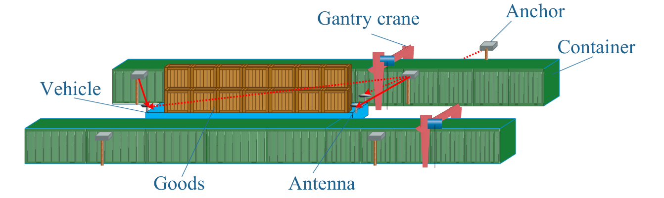
There are $M$ anchors and $N$ antennas in this positioning system. We take the output time of each set of TOA measurements at the antennas as an epoch. Let $\mathcal{N}$ be the set of antennas with $\mathrm{card(\mathcal{N})}=N$, $\mathcal{M}$ be the set of anchors with $\mathrm{card(\mathcal{M})}=M$, and $\mathcal{M}_{i(k)}$ be the set of visible anchors of antenna $i$ at epoch $k$ with $\mathrm{card}\left(\mathcal{M}_{i(k)}\right)=M_{i(k)}$ , $\mathcal{M}_{i(k)}\subseteq\mathcal{M}$.

Without loss of generality, we assume that the vehicle runs on a flat area without changing the height, roll angle and pitch angle. Therefore, the height $h$, roll angle $\gamma$ and pitch angle $\phi$ are regarded as known constants.

The known positions of the anchors and the unknown position of the vehicle are all expressed in the navigation frame, denoted by frame $\mathrm{n}$. We define the body frame with the center of the vehicle platform as the origin, denoted by frame $\mathrm{b}$, which changes with the movement of the vehicle and is expressed as $\mathrm{b}_{(k)}$ at epoch $k$.

We denote the unknown position of the reference point on the vehicle by $\bm{p}_{\mathrm{c}(k)}$, the unknown position of antenna $i$ by $\bm{p}_{i(k)}$, and the known position of anchor $j$ by $\bm{p}_{(k)}^{(j)}$, respectively in frame $\mathrm{n}$. The subscript “$(k)$” represents the epoch index $k$. For simplicity, we do not specify frame $\mathrm{n}$ in the notations. Since the known local positions of the antennas in frame $\mathrm{b}_{(k)}$ do not change when the vehicle moves, we denote it by $\bm{l}_{i}$ without specifying frame $\mathrm{b}$ and epoch $k$.

The relation between the antenna position $\bm{p}_{i(k)}$ in frame $\mathrm{n}$, the position of the reference point of the vehicle $\bm{p}_{\mathrm{c}{(k)}}$ in frame $\mathrm{n}$, and the antenna position $\bm{l}_{i}$ in frame $\mathrm{b}$ is [39]

where $\bm{R}_{(k)}$ is the rotation matrix from frame $\mathrm{b}_{(k)}$ to frame $\mathrm{n}$. See Appendix A for the detailed definition of the rotation matrix.

In this two-dimensional (2D) case, $\bm{R}_{(k)}$ is a function of the yaw angle, denoted by $\psi_{(k)}$, and $\bm{p}_{\mathrm{c}{(k)}}=\left[x_{(k)},\ y_{(k)},\ h\right]^{T}$. The parameter to be estimated, denoted by $\bm{\theta}_{(k)}$, is

In this paper, we consider only the TOA measurements from LOS paths and ignore the non-LOS measurements, which can be identified and eliminated [50, 51, 52, 53]. Following the model of the singe-epoch and single-antenna TOA measurement in [32], we extend it to the multi-epoch and multi-antenna case as

where $\rho_{i(k)}^{(j)}$ is the TOA measurement for antenna $i$ from its $j$-th visible anchor at epoch $k$, $\delta t_{(k)}$ is the common clock bias between all the synchronous antennas and all the synchronous anchors at epoch $k$, and $\varepsilon^{(j)}_{i(k)}$ is the measurement noise, which is independent and identically distributed Gaussian white noise, i.e., $\varepsilon^{(j)}_{i(k)}\sim\mathrm{N}(0,\sigma^{2})$.

The changes of the vehicle position and attitude relative to the previous epochs can be measured by sensors such as the inertial measurement unit (IMU) and odometer in practice [3]. We employ this information as a constraint for the vehicle position.

We model the inter-epoch position and attitude change constraint as

where $\Delta\bm{\theta}_{(k,k-1)}^{\mathrm{b}_{(k-1)}}=\left[\Delta x_{(k,k-1)}^{\mathrm{b}_{(k-1)}},\ \Delta y_{(k,k-1)}^{\mathrm{b}_{(k-1)}},\ \Delta\psi_{(k,k-1)}^{\mathrm{b}_{(k-1)}}\right]^{T}$ is the position and attitude change at epoch $k$ relative to epoch $(k-1)$ in frame $\mathrm{b}_{(k-1)}$, $\Delta\tilde{\bm{\theta}}_{(k,k-1)}^{\mathrm{b}_{(k-1)}}$ is the measurement of $\Delta\bm{\theta}_{(k,k-1)}^{\mathrm{b}_{(k-1)}}$. A number of sensors such as odometer, magnetometer or encoder disk can be adopted to provide the measurements of inter-epoch position and attitude change constraint. We model the measurement errors as Gaussian noises since we do not specify any particular sensor and the characteristics of the sensor are not exactly known. $\bm{\varepsilon}_{\mathrm{IP}(k)}=\left[\varepsilon_{x_{(k)}},\ \varepsilon_{y_{(k)}},\ \varepsilon_{\psi_{(k)}}\right]^{T}$ denotes the noise vector, in which the noises of the inter-epoch position change are modeled as independent and identically distributed Gaussian random variables as $\varepsilon_{x_{(k)}},\varepsilon_{y_{(k)}}\sim\mathrm{N}(0,\sigma_{p}^{2})$, and the inter-epoch yaw angle change noise is modeled as a Gaussian random variable as $\varepsilon_{\psi_{(k)}}\sim\mathrm{N}(0,\sigma_{\psi}^{2})$ [54].

The positioning problem is to estimate $\bm{\theta}_{(k)}$ at each epoch by using the multi-epoch and multi-antenna TOA and inter-epoch constraints. The difficulties of solving this problem lie in the initialization and the location ambiguity removal.

Firstly, the positioning problem is a nonlinear and non-convex optimization problem. Solving this problem based on the iterative MLE achieves the asymptotic optimality, on the condition that it has an accurate initial guess to start the iteration. Otherwise, the iteration may not converge or will be trapped at a local minimum [37, 31].

In addition, ambiguity of locations may appear when the number of TOA measurements is insufficient or the geometry of the observed anchors is inappropriate in harsh environments. These ambiguous solutions are also feasible solutions to the problem, but will lead to unacceptable errors if they are mistaken as the positioning results. For a regional positioning system, the difference between feasible solutions may be very small, sometimes only at meter level or even decimeter level. Therefore, it is difficult to identify the wrong solutions [33, 34].

Fig. 2 gives an example of location ambiguity. Four ambiguous but feasible solutions for the position of the center of the rectangle can be obtained by using the 6 TOA measurements from 4 anchors obtained by 3 antennas. As we can see in Fig. 2, the 4 solutions are so close to each other that it is difficult to identify the correct one without extra information. Therefore, we introduce measurements of multiple epochs to solve this problem, such that a unique solution can be determined without increasing the number of anchors.

To tackle the initialization and location ambiguity issue in the position determination problem, a new MEMA-TOA method, which estimates the parameter $\bm{\theta}_{(k)}$ using the MEMA TOA along with inter-epoch constraints, is proposed in the next section.

We first eliminate the influence of clock bias, by selecting one of the TOA measurements as reference for each epoch (e.g., the measurement between the 1st antenna and its 1st visible anchor is chosen as the reference here, without loss of generality). We subtract (2) plugged with $i=1$ and $j=1$, from (2) with other $i$ and $j$, and come to the time difference of arrival (TDOA) measurement with respect to this reference as written by

where $\Delta\rho_{i1(k)}^{(j1)}$ is the TDOA measurement and the noise term $\Delta\varepsilon^{(j1)}_{i1(k)}=\varepsilon^{(j)}_{i(k)}-\varepsilon^{(1)}_{1(k)}$.

All measurement equations of epoch $k$ as given by (III-A) are written in the collective form as

where

and $\bm{g}_{(k)}\left(\bm{\theta}_{(k)}\right)$ and $\Delta\bm{\varepsilon}_{(k)}$ are the corresponding vectors of the TDOA measurement function and noise at epoch $k$, respectively. The covariance matrix of $\Delta\bm{\varepsilon}_{(k)}$ is $\bm{Q}_{\Delta\bm{\varepsilon}_{(k)}}=\bm{E}_{(k)}\left(\sigma^{2}\bm{I}_{L_{(k)}+1}\right)\bm{E}_{(k)}^{T}$, where $\bm{E}_{(k)}=\left[-\bm{1}_{{L}_{(k)}},\ \bm{I}_{{L}_{(k)}}\right]$, $L_{(k)}=\sum_{i=1}^{N}M_{i(k)}-1$ is the total number of TDOA measurements for $N$ antennas at epoch $k$, $\bm{1}_{{L}_{(k)}}$ is an ${L}_{(k)}$-element column vector with all-one elements, and $\bm{I}_{{L}_{(k)}}$ is an ${{L}_{(k)}}\times{{L}_{(k)}}$ identity matrix.

In order to employ the inter-epoch position and attitude change constraint, we conduct the transformation from frame $\mathrm{n}$ to frame $\mathrm{b}$ for the vehicle position change as given by

By plugging (III-A), the inter-epoch constraints given by (3) are then rewritten as

To simplify the expression, we rewrite (7) into the collective form as

where the subscript “$\mathrm{IP}$” stands for inter-epoch constraints, $\bm{g}_{\mathrm{IP(k)}}$ is a vector of the functions of $\bm{\theta}_{(k)}$ and $\bm{\theta}_{(k-1)}$ as presented in (7), $\Delta\tilde{\bm{\theta}}_{(k,k-1)}^{\mathrm{b}_{(k-1)}}$ and $\bm{\varepsilon}_{\mathrm{IP}(k)}$ are the vectors of the inter-epoch constraints and the corresponding noise at epoch $k$, respectively, and the covariance matrix of $\bm{\varepsilon}_{\mathrm{IP}(k)}$ is $\bm{Q}_{\bm{\varepsilon}_{\mathrm{IP}(k)}}=\operatorname{diag}\left({\sigma_{p}^{2}},{\sigma_{p}^{2}},{\sigma_{\psi}^{2}}\right)$.

As shown in Fig. 3, the MEMA-TOA method utilizes TOAs from multiple recent epochs by introducing the inter-epoch constraints on the changes of position and attitude. The measurements of $K$ epochs and their inter-epoch constraints are collected, resembling a $K$-length sliding window moving forward one epoch at a time.

For $K$ epochs, we denote the parameters to be estimated by

We then construct the MLE for the MEMA problem, utilizing the TOA measurements (5) and inter-epoch constraints (8), as

where the cost function $\mathtt{J}$ for $K$ epochs is given by (11), in which $\bm{W}_{\mathrm{TOA}(k)}$ and $\bm{W}_{\mathrm{IP}(k)}$ are the weights for the TOA measurements and inter-epoch constraints, respectively, and both are determined by their noise covariance as $\bm{W}_{\mathrm{TOA(k)}}=\bm{Q}_{\Delta\bm{\varepsilon}_{(k)}}^{-1}$ and $\bm{W}_{\mathrm{IP}(k)}=\bm{Q}_{\bm{\varepsilon}_{\mathrm{IP}(k)}}^{-1}$.

Note that the cost function $\mathtt{J}$ consists of two parts: $\mathtt{J}_{\mathrm{TOA}}$ relating to the TOA measurements and $\mathtt{J}_{\mathrm{IP}}$ relating to the inter-epoch constraints, corresponding to the two summation terms in (11). Different $N$ and $K$ correspond to different cases. When $K=1$ and $N=1$, $\mathtt{J}_{\mathrm{IP}}$ vanishes, and the positioning problem then degenerates to the traditional case, which uses only the single-epoch and single-antenna measurements. This type of positioning problem is suitable for the application with sufficient measurements and no demand on attitude estimate, and has already been covered extensively in many researches such as [32, 55, 56]. When $K=1$ and $N>1$, $\mathtt{J}_{\mathrm{IP}}$ also vanishes. It is a positioning problem based on single-epoch and multi-antenna TOA measurements, and was discussed in [30]. Finally, when $K>1$ and $N>1$, the MEMA TOA measurements and inter-epoch constraints are used for positioning, and the corresponding problem is studied in this paper.

The proposed MEMA-TOA method is divided into two steps. Firstly, we develop an initialization method, namely MEMA-SDP, to obtain an initial guess. Secondly, we develop an iterative algorithm to refine the estimates based on the initial guess.

Due to the non-convexity of the original optimization problem in (10), finding the exactly optimal solution is challenging. In general, although an MLE is asymptotically efficient and does not depend on the initial guess, its iterative implementation for this positioning problem requires an accurate initial guess to avoid being trapped at a local minimum [57, 31, 37].

SDP can achieve the global optimal solution of an approximate convex problem [58, 59, 31, 38], which is transformed from the original positioning problem by SDR and other approximations. To obtain a proper initialization, we transform and relax $\mathtt{J}_{\mathrm{TOA}}$ and $\mathtt{J}_{\mathrm{IP}}$ to form an SDP problem and then achieve the global optimal solution as an initial guess for the next step.

References

- [1] T. Le-Anh and M. Koster, “A review of design and control of automated guided vehicle systems,” Eur.j.oper.res, vol. 171, no. 1, pp. 1–23, 2006.
- [2] Z. Chen, X. He, Z. Cao, Y. Jin, and J. Li, “Position estimation of automatic-guided vehicle based on MIMO antenna array,” Electronics, vol. 7, no. 9, p. 193, 2018.
- [3] S. A. Mohamed, M.-H. Haghbayan, T. Westerlund, J. Heikkonen, H. Tenhunen, and J. Plosila, “A survey on odometry for autonomous navigation systems,” IEEE Access, vol. 7, pp. 97 466–97 486, 2019.
- [4] A. B. Chatfield, Fundamentals of high accuracy inertial navigation. Aiaa, 1997, vol. 174.
- [5] B. Wang, Z. Deng, C. Liu, Y. Xia, and M. Fu, “Estimation of information sharing error by dynamic deformation between inertial navigation systems,” IEEE Trans. Ind. Electron., vol. 61, no. 4, pp. 2015–2023, 2013.
- [6] W. Li, W. Li, X. Cui, S. Zhao, and M. Lu, “A tightly coupled RTK/INS algorithm with ambiguity resolution in the position domain for ground vehicles in harsh urban environments,” Sensors, vol. 18, no. 7, p. 2160, 2018.
- [7] T. Taketomi, H. Uchiyama, and S. Ikeda, “Visual SLAM algorithms: a survey from 2010 to 2016,” IPSJ T Comput Vis Appl, vol. 9, no. 1, pp. 1–11, 2017.
- [8] C. Cadena, L. Carlone, H. Carrillo, Y. Latif, D. Scaramuzza, J. Neira, I. Reid, and J. J. Leonard, “Past, present, and future of simultaneous localization and mapping: Toward the robust-perception age,” IEEE Trans. Robot., vol. 32, no. 6, pp. 1309–1332, 2016.
- [9] H. Durrant-Whyte and T. Bailey, “Simultaneous localization and mapping: Part I,” IEEE Robot Autom Mag, vol. 13, no. 2, pp. 99–110, 2006.
- [10] A. Y. Hata and D. F. Wolf, “Feature detection for vehicle localization in urban environments using a multilayer LIDAR,” IEEE Transactions on Intelligent Transportation Systems, vol. 17, no. 2, pp. 420–429, 2016.
- [11] L. Zamora-Cadenas, I. Velez, and J. E. Sierra-Garcia, “UWB-based safety system for autonomous guided vehicles without hardware on the infrastructure,” IEEE Access, pp. 1–1, 2021.
- [12] I. Guvenc, S. Gezici, and Z. Sahinoglu, “Ultra-wideband range estimation: Theoretical limits and practical algorithms,” in 2008 IEEE International Conference on Ultra-Wideband (ICUWB), vol. 3. IEEE, 2008, pp. 93–96.
- [13] Y. Shen and M. Z. Win, “Fundamental limits of wideband localization—Part I: A general framework,” IEEE Trans. Inf. Theory, vol. 56, no. 10, pp. 4956–4980, 2010.
- [14] S. Zhao, X.-P. Zhang, X. Cui, and M. Lu, “Optimal two-way TOA localization and synchronization for moving user devices with clock drift,” IEEE Trans. Veh. Technol., 2021.
- [15] S. Zhao, Z. Yao, X. Zhuang, and M. Lu, “Analysis on coverage ability of BeiDou navigation satellite system for manned spacecraft,” Acta Astronautica, vol. 105, no. 2, pp. 487–494, 2014.
- [16] S. Zhao, X.-P. Zhang, X. Cui, and M. Lu, “Optimal localization with sequential pseudorange measurements for moving users in a time-division broadcast positioning system,” IEEE Internet Things J., vol. 8, no. 11, pp. 8883–8896, 2021.
- [17] P. Fan, X. Cui, S. Zhao, G. Liu, and M. Lu, “A two-step stochastic hybrid estimation for GNSS carrier phase tracking in urban environments,” IEEE Trans. Instrum. Meas., 2021.
- [18] C. M. Zhang, M. Kuhn, B. Merkl, A. E. Fathy, and M. Mahfouz, “Accurate UWB indoor localization system utilizing time difference of arrival approach,” in Radio & Wireless Symposium, 2006.
- [19] V. Djaja-Josko, J. Kolakowski, and J. Modelski, “TDOA estimation using a pair of synchronized DW1000 based anchor nodes,” in 2018 22nd International Microwave and Radar Conference (MIKON), 2018, pp. 57–60.
- [20] Q. Shi, X. Cui, S. Zhao, S. Xu, and M. Lu, “BLAS: Broadcast relative localization and clock synchronization for dynamic dense multi-agent systems,” IEEE Trans. Aerosp. Electron. Syst., pp. 1–1, 2020.
- [21] H. Matsumoto, H. Kusano, T. Morokuma, and K. Sakamura, “Numerical and experimental investigation of TDOA-based positioning system by ultra-wideband impulse radio,” in 2011 IEEE Topical Conference on Wireless Sensors and Sensor Networks, 2011, pp. 25–28.
- [22] J. Sidorenko, V. Schatz, N. Scherer-Negenborn, M. Arens, and U. Hugentobler, “Error corrections for ultrawideband ranging,” IEEE Trans. Instrum. Meas., vol. 69, no. 11, pp. 9037–9047, 2020.
- [23] J. Tiemann, F. Eckermann, and C. Wietfeld, “ATLAS - an open-source TDOA-based ultra-wideband localization system,” in 2016 International Conference on Indoor Positioning and Indoor Navigation (IPIN), 2016.
- [24] G. Soatti, M. Nicoli, N. Garcia, B. Denis, R. Raulefs, and H. Wymeersch, “Implicit cooperative positioning in vehicular networks,” IEEE Trans. Intell. Transp. Syst., vol. 19, no. 12, pp. 3964–3980, 2018.
- [25] H. Wymeersch, J. Lien, and M. Z. Win, “Cooperative localization in wireless networks,” Proc. IEEE, vol. 97, no. 2, pp. 427–450, 2009.
- [26] T. V. Nguyen, Y. Jeong, H. Shin, and M. Z. Win, “Least square cooperative localization,” IEEE Trans. Veh. Technol., vol. 64, no. 4, pp. 1318–1330, 2015.
- [27] B. Huang, Z. Yao, X. Cui, and M. Lu, “Dilution of precision analysis for GNSS collaborative positioning,” IEEE Trans. Veh. Technol., vol. 65, no. 5, pp. 3401–3415, 2015.
- [28] F. Lobo, D. Grael, H. Oliveira, L. Villas, A. Almehmadi, and K. El-Khatib, “Cooperative localization improvement using distance information in vehicular ad hoc networks,” Sensors, vol. 19, no. 23, p. 5231, 2019.
- [29] S. Wang and X. Jiang, “Three-dimensional cooperative positioning in vehicular ad-hoc networks,” IEEE Trans. Intell. Transp. Syst., vol. 22, no. 2, pp. 937–950, 2021.
- [30] X. An, S. Zhao, X. Cui, Q. Shi, and M. Lu, “Distributed multi-antenna positioning for automatic-guided vehicle,” Sensors, vol. 20, no. 4, p. 1155, 2020.
- [31] S. Zhao, X.-P. Zhang, X. Cui, and M. Lu, “Semidefinite programming two-way TOA localization for user devices with motion and clock drift,” IEEE Signal Process. Lett., vol. 28, pp. 578–582, 2021.
- [32] E. Kaplan and C. Hegarty, Understanding GPS: principles and applications. Artech house, 2005.
- [33] A. A. Kannan, B. Fidan, and G. Mao, “Analysis of flip ambiguities for robust sensor network localization,” IEEE Trans. Veh. Technol., vol. 59, no. 4, pp. 2057–2070, 2010.
- [34] P. Moravek, D. Komosny, M. Simek, and J. Muller, “Multilateration and flip ambiguity mitigation in ad-hoc networks,” Przeglad Elektrotechniczny, vol. 2012, no. 05b, pp. 222–229, 2012.
- [35] S. Chen and K. C. Ho, “Accurate localization of a rigid body using multiple sensors and landmarks,” IEEE Trans. Signal Process., vol. 63, no. 24, pp. 6459–6472, 2015.
- [36] J. Jiang, G. Wang, and K. C. Ho, “Accurate rigid body localization via semidefinite relaxation using range measurements,” IEEE Signal Process. Lett., vol. 25, no. 3, pp. 378–382, 2018.
- [37] ——, “Sensor network-based rigid body localization via semi-definite relaxation using arrival time and Doppler measurements,” IEEE Trans. Wirel. Commun., vol. 18, no. 2, pp. 1011–1025, 2019.
- [38] X. Ke, Y. Wang, and L. Huang, “Three-dimensional rigid body localization in the presence of clock offsets,” IEEE Signal Process. Lett., vol. 27, pp. 96–100, 2020.
- [39] J. Farrell, Aided navigation: GPS with high rate sensors. McGraw-Hill, Inc., 2008.
- [40] S. V. S. Chauhan and G. X. Gao, “Joint GPS and vision estimation using an adaptive filter,” in Proceedings of the 30th International Technical Meeting of the Satellite Division of the Institute of Navigation (ION GNSS+ 2017), 2017, pp. 808–812.
- [41] G. Ding, H. Lu, J. Bai, and X. Qin, “Development of a high precision UWB/vision-based AGV and control system,” in 2020 5th International Conference on Control and Robotics Engineering (ICCRE), 2020, pp. 99–103.
- [42] E. I. Laftchiev, C. M. Lagoa, and S. N. Brennan, “Vehicle localization using in-vehicle pitch data and dynamical models,” IEEE Trans. Intell. Transp. Syst., vol. 16, no. 1, pp. 206–220, 2015.
- [43] Y. Wang, X. Zhao, C. Pang, B. Feng, and L. Zhang, “The influence of attitude dilution of precision on the observable degree and observability analysis with different numbers of visible satellites in a multi-antenna GNSS/INS attitude determination system,” IEEE Access, pp. 1–1, 2018.
- [44] H. Fang, M. A. Haile, and Y. Wang, “Robust extended Kalman filtering for systems with measurement outliers,” IEEE Trans. Control Syst. Technol., vol. 30, no. 2, pp. 795–802, 2022.
- [45] A. H. Chughtai, U. Akram, M. Tahir, and M. Uppal, “Dynamic state estimation in the presence of sensor outliers using MAP-based EKF,” IEEE Sensors Letters, vol. PP, no. 99, pp. 1–1, 2020.
- [46] J. Brembeck, “Nonlinear constrained moving horizon estimation applied to vehicle position estimation,” Sensors, vol. 19, no. 10, p. 2276, 2019.
- [47] S. Zhao, Y. Chen, and J. A. Farrell, “High-precision vehicle navigation in urban environments using an MEM’s IMU and single-frequency GPS receiver,” IEEE Trans. Intell. Transp. Syst., vol. 17, no. 10, pp. 2854–2867, 2016.
- [48] K. Yu, I. Sharp, and Y. J. Guo, Ground‐Based Wireless Positioning. Wiley-IEEE Press., 2009.
- [49] S. Zhao, X.-P. Zhang, X. Cui, and M. Lu, “A new TOA localization and synchronization system with virtually synchronized periodic asymmetric ranging network,” IEEE Internet Things J., vol. 8, no. 11, pp. 9030–9044, 2021.
- [50] P. D. Groves, Z. Jiang, B. Skelton, P. A. Cross, L. Lau, Y. Adane, and I. Kale, “Novel multipath mitigation methods using a dual-polarization antenna,” in Proceedings of the 23rd International Technical Meeting of The Satellite Division of the Institute of Navigation (ION GNSS 2010), 2010, pp. 140–151.
- [51] B. Xu, Q. Jia, and L.-T. Hsu, “Vector tracking loop-based GNSS NLOS detection and correction: Algorithm design and performance analysis,” IEEE Trans. Instrum. Meas., vol. 69, no. 7, pp. 4604–4619, 2020.
- [52] K. Yu, K. Wen, Y. Li, S. Zhang, and K. Zhang, “A novel NLOS mitigation algorithm for UWB localization in harsh indoor environments,” IEEE Trans. Veh. Technol., vol. 68, no. 1, pp. 686–699, 2019.
- [53] L. Cong and W. Zhuang, “Nonline-of-sight error mitigation in mobile location,” IEEE Trans. Wireless Commun., vol. 4, no. 2, pp. 560–573, 2005.
- [54] Q. Chen, Q. Zhang, and X. Niu, “Estimate the pitch and heading mounting angles of the IMU for land vehicular GNSS/INS integrated system,” IEEE Trans. Intell. Transp. Syst., pp. 1–13, 2020.
- [55] Z. Sahinoglu, S. Gezici, and I. Gvenc, Ultra-Wideband Positioning Systems: Theoretical Limits, Ranging Algorithms, and Protocols. USA: Cambridge University Press, 2011.
- [56] J. Shen, A. F. Molisch, and J. Salmi, “Accurate passive location estimation using TOA measurements,” IEEE Trans. Wireless Commun., vol. 11, no. 6, pp. 2182–2192, 2012.
- [57] S. M. Kay, Fundamentals of Statistical Signal Processing: Estimation Theory. PTR Prentice-Hall, 1993.
- [58] G. Wang, A. M.-C. So, and Y. Li, “Robust convex approximation methods for TDOA-based localization under NLOS conditions,” IEEE Trans. Signal Process., vol. 64, no. 13, pp. 3281–3296, 2016.
- [59] Z. Su, G. Shao, and H. Liu, “Semidefinite programming for NLOS error mitigation in TDOA localization,” IEEE Commun. Lett., vol. 22, no. 7, pp. 1430–1433, 2017.
- [60] R. A. Horn and C. R. Johnson, Matrix analysis. Cambridge university press, 2012.
- [61] S. Boyd and L. Vandenberghe, Convex Optimization. Cambridge university press, 2004.
- [62] D. P. Bertsekas, Nonlinear Programming 2nd edn. Belmont, Mass. : Athena Scientific, 1999.
- [63] A. Ben-Tal and A. Nemirovski, Lectures on modern convex optimization: analysis, algorithms, and engineering applications. SIAM, 2001.
- [64] P. Biswas, T.-C. Lian, T.-C. Wang, and Y. Ye, “Semidefinite programming based algorithms for sensor network localization,” ACM Trans. Sen. Netw., vol. 2, no. 2, p. 188–220, may 2006. [Online]. Available: https://doi.org/10.1145/1149283.1149286
- [65] E. S. Quintana, G. Quintana, X. Sun, and R. van de Geijn, “A note on parallel matrix inversion,” SIAM Journal on Scientific Computing, vol. 22, no. 5, pp. 1762–1771, 2001.
- [66] M. Grant and S. Boyd, “CVX: Matlab software for disciplined convex programming, version 2.1,” http://cvxr.com/cvx, Mar. 2014.
- [67] J. F. Sturm, “Using SeDuMi 1.02, a MATLAB toolbox for optimization over symmetric cones,” Optim. Methods Softw., vol. 11, no. 1-4, 1999.
- [68] DW1000 User Manual, Decawave Ltd., Dublin, Ireland, 2015.
- [69] S. Pala, S. Jayan, and D. G. Kurup, “An accurate UWB based localization system using modified leading edge detection algorithm,” Ad Hoc Networks, vol. 97, p. 102017, 2020.