跳到论文正文
W Papers独立论文阅读器 arXiv:2207.07542 论文正文 计算阅读时间 · 0%
引用这篇论文根据当前论文元数据生成,正式投稿前建议核对。


License: arXiv.org perpetual non-exclusive license
arXiv:2207.07542v2 [math.NA] 01 Jun 2023

Least squares solvers for ill-posed PDEs that are conditionally stableThanks: This research has been supported in part by the NSF Grant DMS ID 2012469, by the SmartState and Williams-Hedberg Foundation, by the SFB 1481, funded by the German Research Foundation, and by the Netherlands Organization for Scientific Research (NWO) under contract. no. SH-208-11. We acknowledge the support of SURF (www.surf.nl) in using the National Supercomputer Snellius.

Wolfgang Dahmen Address: Mathematics Department, University of South Carolina, Columbia SC 29208 Email address: wolfgang.anton.dahmen@googlemail.com , Harald Monsuur and Rob Stevenson Address: Korteweg-de Vries (KdV) Institute for Mathematics, University of Amsterdam, P.O. Box 94248, 1090 GE Amsterdam, The Netherlands. Email address: h.monsuur@uva.nl, rob.p.stevenson@gmail.com
Date: August 11, 2026
Abstract.

This paper is concerned with the design and analysis of least squares solvers for ill-posed PDEs that are conditionally stable. The norms and the regularization term used in the least squares functional are determined by the ingredients of the conditional stability assumption. We are then able to establish a general error bound that, in view of the conditional stability assumption, is qualitatively the best possible, without assuming consistent data. The price for these advantages is to handle dual norms which reduces to verifying suitable inf-sup stability. This, in turn, is done by constructing appropriate Fortin projectors for all sample scenarios. The theoretical findings are illustrated by numerical experiments.

Key words and phrases: 
Tikhonov regularization, least squares methods, conditional stability, dual norms, inf-sup stability, Fortin projectors, mixed formulations, a posteriori bounds for residuals
2020 Mathematics Subject Classification
35B30 35B35 35B45, 35R25, 65F08, 65J20, 65M12, 65N12

1. Introduction

In this paper a general approach is developed for the numerical solution of ill-posed boundary value problems A​u=fAu=f, where A∈ℒ⁡(X,V)A\in\mathcal{L}(X,V) for Hilbert spaces XX and VV, that are conditionally stable. The latter means that for all u∈Xu\in X that satisfy an a priori bound of the form ‖L​u‖H≤C\|Lu\|_{H}\leq C, for some L∈ℒ⁡(X,H)L\in\mathcal{L}(X,H) and a Hilbert space HH, there is a continuous dependency of the solution on the data in the sense that, for some η=ηC:ℝ+→ℝ+\eta=\eta_{C}\colon\mathbb{R}^{+}\rightarrow\mathbb{R}^{+} with limt↓0η⁡(t)=0\lim_{t\downarrow 0}\eta(t)=0, it holds that j⁡(u)≤η⁡(‖A​u‖V)j(u)\leq\eta\big(\|Au\|_{V}\big) for some j:X→ℝ+j\colon X\rightarrow\mathbb{R}_{+}. In applications j⁡(⋅)j(\cdot) is a (semi-) norm that is weaker than the norm on XX, and, e.g., η⁡(t)=ts\eta(t)=t^{s} or even only η(t)=(−1/logt)s\eta(t)=(-1/\log t)^{s} for some s∈(0,1]s\in(0,1]. Conditional stability has been established for various ill-posed PDEs including data-assimilation and Cauchy boundary data problems for Poisson’s, heat and wave equations.

For finite dimensional subspaces Xδ⊂XX^{\delta}\subset X (‘δ\delta’ refers to ‘discrete’), we approximate uu by the minimizer uεδu_{\varepsilon}^{\delta} over XδX^{\delta} of the regularized least-squares functional z↦‖A​z−f‖V2+ε2​‖L​z‖H2z\mapsto\sqrt{\|Az-f\|_{V}^{2}+\varepsilon^{2}\|Lz\|_{H}^{2}}. For a suitable selection of ε\varepsilon, it will be shown that both ‖L⁡(u−uεδ)‖H\|L(u-u_{\varepsilon}^{\delta})\|_{H} is uniformly bounded, so that j⁡(u−uεδ)≤η⁡(‖f−A​uεδ‖V)j(u-u_{\varepsilon}^{\delta})\leq\eta\big(\|f-Au_{\varepsilon}^{\delta}\|_{V}\big), and ‖f−A​uεδ‖V\|f-Au_{\varepsilon}^{\delta}\|_{V} is bounded by an absolute multiple of ‖f−A​u‖V+minz∈Xδ⁡‖u−z‖X\|f-Au\|_{V}+\min_{z\in X^{\delta}}\|u-z\|_{X}, being the sum of the consistency error and the error of best approximation. Consequently, we will achieve qualitatively the best possible bound on the error quantity j⁡(u−uεδ)j(u-u_{\varepsilon}^{\delta}) that can be expected for uεδ∈Xδu_{\varepsilon}^{\delta}\in X^{\delta} in view of the conditional stability estimate.

In applications often VV is of product form ∏iVi\prod_{i}V_{i}, and so A=(Ai)A=(A_{i}) and f=(fi)f=(f_{i}), with one or more ViV_{i} being a Sobolev space with negative smoothness index, which is a natural space for a forcing term of a PDE, or a fractional Sobolev space on (a part of) the boundary of the computational domain, which is a natural space for a boundary datum. The norms on such spaces cannot be evaluated exactly.

An option to deal with a Sobolev norm of negative smoothness index is to replace it by an L2L_{2}-norm. This, however, requires more smoothness of the data and more regularity of XδX^{\delta}, e.g., a C1C^{1}- instead of a C0C^{0}-finite element space, whereas it is not ensured that the error benefits from smallness of the residual in a stronger norm. Similar disadvantages are connected to the replacement of fractional Sobolev norms by (weighted) L2L_{2}-norms.

Our approach to deal with ViV_{i} being a Sobolev space with negative smoothness index, i.e., a ViV_{i} being of the form Yi′Y_{i}^{\prime}, is to replace ∥⋅∥Yi′\|\cdot\|_{Y_{i}^{\prime}} in the least-squares functional by a discrete dual norm ∥⋅∥Yiδ′\|\cdot\|_{{Y^{\delta}_{i}}^{\prime}}, where Yiδ=Yiδ​(Xδ)⊂YiY_{i}^{\delta}=Y_{i}^{\delta}(X^{\delta})\subset Y_{i} is such that ∥Ai⋅∥Yi′\|A_{i}\cdot\|_{Y_{i}^{\prime}} is equivalent to ∥Ai⋅∥Yiδ′\|A_{i}\cdot\|_{{Y^{\delta}_{i}}^{\prime}} on XδX^{\delta}, and dimYiδ\dim Y_{i}^{\delta} is proportional to dimXδ\dim X^{\delta}. The first property is known to be equivalent to existence of a (uniformly bounded) Fortin projector Yi→YiδY_{i}\rightarrow Y_{i}^{\delta}.

By introducing the Riesz lift of the corresponding residual fi−Ai​uεδ∈Yiδ′f_{i}-A_{i}u^{\delta}_{\varepsilon}\in{Y_{i}^{\delta}}^{\prime} as an independent variable, the resulting least squares problem has an equivalent formulation as a mixed system, which does not involve the dual norm ∥⋅∥Yiδ′\|\cdot\|_{{Y^{\delta}_{i}}^{\prime}}, and which is Ladyshenskaja-Babus̆ka-Brezzi (LBB) stable by virtue of the existence of the Fortin projector. In many cases, one can construct a GYiδ:Yiδ′→YiδG^{\delta}_{Y_{i}}\colon{Y^{\delta}_{i}}^{\prime}\rightarrow Y^{\delta}_{i} (known as a preconditioner) with (GYiδ−1​v)​(v)({G^{\delta}_{Y_{i}}}^{-1}v)(v) equivalent to ‖v‖Yi2\|v\|_{Y_{i}}^{2}, and whose application can be performed in linear complexity, in which case one can efficiently eliminate the additional variable and so retrieves a symmetric positive definite system.

We handle fractional Sobolev norms in the same manner. Viewing a fractional Sobolev space ViV_{i}, with either a positive or negative smoothness index, as the dual of Yi:=Vi′Y_{i}:=V_{i}^{\prime}, first we construct a (uniformly bounded) Fortin projector Yi→YiδY_{i}\rightarrow Y_{i}^{\delta}, and second, to avoid having to compute fractional norms with opposite index of arguments from YiδY_{i}^{\delta}, we use a preconditioner GYiδ:Yiδ′→YiδG^{\delta}_{Y_{i}}\colon{Y^{\delta}_{i}}^{\prime}\rightarrow Y^{\delta}_{i} with (GYiδ−1​v)​(v)({G^{\delta}_{Y_{i}}}^{-1}v)(v) equivalent to ‖v‖Yi2\|v\|_{Y_{i}}^{2}.

The steps to handle dual or fractional norms, mentioned above, make our approach practically feasible without compromizing its attractive theoretical properties. Indeed, still one obtains a bound on the error quantity j⁡(u−uεδ)j(u-u_{\varepsilon}^{\delta}) that is qualitatively the best possible.

We exemplify our approach by constructing Fortin interpolators and preconditioners for the examples of the Cauchy problem for Poisson’s equation, and data-assimilation problems for wave- and heat-equations. Furthermore, for those examples we illustrate our theoretical findings with numerical results.

Our approach to minimize a regularized least squares functional is of course not new. Not making use of conditional stability, in [BBFD15, BR18, BC20] this method was analyzed for a regularizing term ε2​‖z‖X2\varepsilon^{2}\|z\|_{X}^{2}, instead of our choice ε2​‖L​z‖H2\varepsilon^{2}\|Lz\|_{H}^{2} suggested by the conditional stability condition. By replacing the test function from XX by minus this test function, a non-symmetric mixed system on X×VX\times V is obtained that is coercive, with a coercivity constant that is, however, proportional to ε2\varepsilon^{2}. With this formulation the notion of stability is fully due to the stabilization term. By our approach to guarantee LBB-stability, the operator AA contributes to the stability of the least-squares problem. It results in a proof of convergence rates in the error quantity associated to the conditional stability estimate that seems new.

The use of conditional stability estimates for the numerical solution of various ill-posed PDEs has been advocated in series of papers [Bur16, BFO20, BFMO21a, BO18, BIHO18, BHL18, Bur17, BFMO21b, BDE22]. In those works a control functional is minimized under the constraint that the state satisfies the PDE. Instead of adding Tikhonov stabilization at the continuous level, mesh-dependent stabilization terms tailored to the application at hand are added to the finite element discretization.

1.1. Layout

In Sect. 2 we recall the concept of conditional stability for ill–posed problems A​u=fAu=f. Under the provision that approximations uεδu_{\varepsilon}^{\delta} to uu from finite dimensional spaces XδX^{\delta} are available that satisfy a certain quasi-optimal error bound in an ε\varepsilon-dependent energy norm, it will be demonstrated that, for a judiciously chosen regularization parameter ε\varepsilon, a qualitatively best possible upper bound holds for the error quantity j⁡(u−uεδ)j(u-u_{\varepsilon}^{\delta}). In Sect. 3 we present several classical examples to which the theory applies. In Sect. 4 the aforementioned quasi-optimal error bound will be demonstrated for uεδ∈Xδu_{\varepsilon}^{\delta}\in X^{\delta} being the minimizer of a regularized least squares functional, in which, under inf-sup conditions, dual norms are replaced by discrete dual norms. The resulting least-squares problem has an equivalent formulation as a mixed system. Sect. 5 is devoted to a reformulation of the mixed problem as a symmetric positive definite variational problem, based on uniform preconditioners that serve as approximate Riesz lifters in those Hilbert space components that require the use of dual norms. In Sect. 6 we discuss a posteriori residual estimators. In Sect. 7 we verify the validity of the critical inf-sup conditions for all sample problems, the results in preceding sections hinge upon. Here the central work horse are suitable Fortin operators. Finally, in Sect. 8 we present numerical results for our three sample problems.

1.2. Notation

In this work, by C≲DC\lesssim D we will mean that CC can be bounded by a multiple of DD, independently of parameters which CC and DD may depend on, as the discretisation index δ\delta, the tolerance τ\tau for the consistency error, and the regularization parameters ε\varepsilon and ζ\zeta. Obviously, C≳DC\gtrsim D is defined as D≲CD\lesssim C, and C≂DC\eqsim D as C≲DC\lesssim D and C≳DC\gtrsim D.

For normed linear spaces EE and FF, by ℒ⁡(E,F)\mathcal{L}(E,F) we will denote the normed linear space of bounded linear mappings E→FE\rightarrow F, and by ℒ​is​(E,F)\mathcal{L}\mathrm{is}(E,F) its subset of boundedly invertible linear mappings E→FE\rightarrow F. We write E↪FE\hookrightarrow F to denote that EE is continuously embedded into FF. For convenience only, we exclusively consider linear spaces over the scalar field ℝ\mathbb{R}.

The set [0,∞)[0,\infty) will be denoted by ℝ+\mathbb{R}^{+}.

2. Problem setting and main result

For Hilbert spaces XX and VV, we consider operators A∈ℒ⁡(X,V)A\in\mathcal{L}(X,V) which are neither assumed to be injective nor to have a dense range in VV. We study the problem of the (approximate) reconstruction of u∈Xu\in X from its image A​uAu assuming we are only given a perturbation ff of A​uAu for which

(2.1) ‖f−A​u‖V≤τ\|f-Au\|_{V}\leq\tau

holds for some tolerance τ≥0\tau\geq 0 which we assume to be known. Since in particular we do not assume bounded invertibility of AA our problem is ill-posed, even for τ=0\tau=0. Although for convenience we refer in the following to uu as the solution of our recovery problem, one should bear in mind that for τ>0\tau>0 there may be multiple u∈Xu\in X that satisfy (2.1). Our results will be valid uniformly in those uu.

Since Tikhonov ([Tik43]) with stability for ill-posed problems, usually called conditional stability, one understands some continuous dependency of the solution upon the data, typically with respect to a weaker metric than that induced by ∥⋅∥X\|\cdot\|_{X}, under the assumption that a bound on the solution itself is available. More specifically, similar to [Bur16], we assume existence of an L∈ℒ⁡(X,H)L\in\mathcal{L}(X,H), where HH is some additional Hilbert space, such that the following assumption is valid:

Assumption 2.1 (Conditional stability).

The pair

(A,L)∈ℒ⁡(X,V×H)​ is injective,(A,L)\in\mathcal{L}(X,V\times H)\,\,\text{ is injective,}

and there exists a j:X→ℝ+j\colon X\rightarrow\mathbb{R}^{+}, and for any 𝒞>0\mathcal{C}>0, a non-decreasing η=η𝒞:ℝ+→ℝ+\eta=\eta_{\mathcal{C}}\colon\mathbb{R}^{+}\rightarrow\mathbb{R}^{+} with limt↓0η⁡(t)=0\lim_{t\downarrow 0}\eta(t)=0, such that for z∈Xz\in X with ‖L​z‖H≤𝒞\|Lz\|_{H}\leq{\mathcal{C}}, it holds that

(2.2) j⁡(z)≤η𝒞​(‖A​z‖V).j(z)\leq\eta_{\mathcal{C}}\big(\|Az\|_{V}\big).

Typically, jj is a norm or a semi-norm on a Hilbert space H~↩X\widetilde{H}\hookleftarrow X. In the first case, AA is injective. Several examples will be given in Sect. 3.

For ε>0\varepsilon>0, we set

(2.3) |||⋅|||ε:=∥A⋅∥V2+ε2∥L⋅∥H2.|\!|\!|\cdot|\!|\!|_{\varepsilon}:=\sqrt{\|A\cdot\|_{V}^{2}+\varepsilon^{2}\|L\cdot\|_{H}^{2}}.

To use precisely the ingredients of the conditional stability condition in the definition of |||⋅|||ε|\!|\!|\cdot|\!|\!|_{\varepsilon} will be seen to be essential in what follows. Moreover, notice that |||⋅|||ε|\!|\!|\cdot|\!|\!|_{\varepsilon} is a norm on XX by our assumption of (A,L)(A,L) being injective. Thinking of ε\varepsilon being small, tacitly we will always assume that ε​‖L‖ℒ⁡(X,H)≲1\varepsilon\|L\|_{\mathcal{L}(X,H)}\lesssim 1 so that, since AA is bounded, |||⋅|||ε≲∥⋅∥X|\!|\!|\cdot|\!|\!|_{\varepsilon}\lesssim\|\cdot\|_{X}.

Given a finite dimensional subspace XδX^{\delta} of XX, in Sect. 4-5 we show how to compute for each ε>0\varepsilon>0 a uεδ∈Xδu_{\varepsilon}^{\delta}\in X^{\delta} satisfying

(2.4) ‖|u−uεδ|‖ε≲τ+minz∈Xδ⁡‖|u−z|‖ε+ε​‖L​u‖H.|\!|\!|u-u_{\varepsilon}^{\delta}|\!|\!|_{\varepsilon}\lesssim\tau+\min_{z\in X^{\delta}}|\!|\!|u-z|\!|\!|_{\varepsilon}+\varepsilon\|Lu\|_{H}.

If (2.2) is valid for L=0L=0, and thus η𝒞≡η\eta_{\mathcal{C}}\equiv\eta is independent of 𝒞{\mathcal{C}}, then one speaks about unconditional stability of (2.1).11 1 Not to be confused with well-posedness, with which we mean A∈ℒ​is​(X,V)A\in\mathcal{L}\mathrm{is}(X,V). An unconditionally stable problem where ran⁡A\ran A is closed is also benign in the sense that then, by an application of the open mapping theorem, (2.1) is well-posed in least-squares sense, i.e., A∗​A∈ℒ​is​(X,X)A^{*}A\in\mathcal{L}\mathrm{is}(X,X), and thus is also not of our primary interest. In this case |||⋅|||ε=∥A⋅∥V|\!|\!|\cdot|\!|\!|_{\varepsilon}=\|A\cdot\|_{V} is ε\varepsilon-independent, and so will be uεδu_{\varepsilon}^{\delta}.

Theorem 2.2.

Assume (2.4) and recall Assumption 2.1. For L≠0L\neq 0, let ε=ε⁡(τ,δ)>0\varepsilon=\varepsilon(\tau,\delta)>0 be such that for some 𝒞≥‖L​u‖H{\mathcal{C}}\geq\|Lu\|_{H},

(2.5) τ+minz∈Xδ⁡‖|u−z|‖ε≲ε​𝒞 and ε​‖L​u‖H≲τ+minz∈Xδ⁡‖u−z‖X.\tau+\min_{z\in X^{\delta}}|\!|\!|u-z|\!|\!|_{\varepsilon}\lesssim\varepsilon{\mathcal{C}}\quad\text{ and }\quad\varepsilon\|Lu\|_{H}\lesssim\tau+\min_{z\in X^{\delta}}\|u-z\|_{X}.

Then

(2.6) j⁡(u−uεδ)≤η𝒞​(‖A⁡(u−uεδ)‖V),j(u-u_{\varepsilon}^{\delta})\leq\eta_{\mathcal{C}}\big(\|A(u-u_{\varepsilon}^{\delta})\|_{V}\big),

and

(2.7) ‖A⁡(u−uεδ)‖V≲τ+minz∈Xδ⁡‖u−z‖X.\|A(u-u_{\varepsilon}^{\delta})\|_{V}\lesssim\tau+\min_{z\in X^{\delta}}\|u-z\|_{X}.
Proof.

When L=0L=0, (2.6) holds unconditionally, and |||⋅|||ε=∥A⋅∥V≲∥⋅∥X|\!|\!|\cdot|\!|\!|_{\varepsilon}=\|A\cdot\|_{V}\lesssim\|\cdot\|_{X} so that (2.7) follows directly from (2.4). So let L≠0L\neq 0. From (2.4) and the lower bound from (2.5) on ε\varepsilon, one derives ‖L⁡(u−uεδ)‖H≤ε−1​‖|u−uεδ|‖ε≲𝒞\|L(u-u_{\varepsilon}^{\delta})\|_{H}\leq\varepsilon^{-1}|\!|\!|u-u_{\varepsilon}^{\delta}|\!|\!|_{\varepsilon}\lesssim{\mathcal{C}}. Conditional stability then ensures

j⁡(u−uεδ)≤η𝒞​(‖A⁡(u−uεδ)‖V).j(u-u_{\varepsilon}^{\delta})\leq\eta_{\mathcal{C}}\big(\|A(u-u_{\varepsilon}^{\delta})\|_{V}\big).

Again (2.4), and the upper bound on ε\varepsilon from (2.5) show that

‖A⁡(u−uεδ)‖V≤‖|u−uεδ|‖ε≲τ+minz∈Xδ⁡‖u−z‖X,\|A(u-u_{\varepsilon}^{\delta})\|_{V}\leq|\!|\!|u-u_{\varepsilon}^{\delta}|\!|\!|_{\varepsilon}\lesssim\tau+\min_{z\in X^{\delta}}\|u-z\|_{X},

which completes the proof.∎

Notice that when minz∈Xδ⁡‖u−z‖X\min_{z\in X^{\delta}}\|u-z\|_{X} in (2.5) is replaced by an upper bound, then one arrives at (2.7) with minz∈Xδ⁡‖u−z‖X\min_{z\in X^{\delta}}\|u-z\|_{X} replaced by that upper bound.

In the examples given in Sect. 3, η𝒞​(t)\eta_{\mathcal{C}}(t) will be of the form 𝒪⁡((t+𝒞)1−σ​tσ){\mathcal{O}}((t+\mathcal{C})^{1-\sigma}t^{\sigma}) or 𝒪⁡((t+𝒞)​(log⁡(1+𝒞t))−σ){\mathcal{O}}((t+\mathcal{C})(\log(1+\frac{{\mathcal{C}}}{t}))^{-\sigma}) for some σ∈(0,1)\sigma\in(0,1), or 𝒪⁡(t){\mathcal{O}}(t).

2.3Optimality of estimates.

The bound (2.7) on ‖A⁡(u−uεδ)‖V\|A(u-u_{\varepsilon}^{\delta})\|_{V}, (valid because of the upper bound on ε\varepsilon), by a multiple of the sum of the (maximal) consistency error τ\tau and the approximation error minz∈Xδ⁡‖u−z‖X\min_{z\in X^{\delta}}\|u-z\|_{X}, is qualitatively the best that can be expected for a numerical approximation from XδX^{\delta}. Since, thanks to the lower bound on ε\varepsilon, at the same time ‖L⁡(u−uεδ)‖H≲𝒞\|L(u-u_{\varepsilon}^{\delta})\|_{H}\lesssim{\mathcal{C}}, we obtain the generally qualitatively best possible upper bound for j⁡(u−uεδ)j(u-u_{\varepsilon}^{\delta}) that is permitted by the conditional stability estimate.

That being said, inserting the upper bound in (2.7) into (2.6) can nevertheless provide a pessimistic bound. The reason is that perturbations in the data enter the approximation by solving a discretized problem, whose conditioning is for coarser and coarser meshes usually increasingly better than that of the infinite dimensional problem whose behaviour is captured by the conditional stability estimate.

2.4Selection of ε\varepsilon when L≠0L\neq 0.

Let (Xδ)(X^{\delta}) be a family of finite dimensional subspaces of XX such that for some s>0s>0 for general, sufficiently smooth u∈Xu\in X it holds minz∈Xδ⁡‖u−z‖X≂(dimXδ)−s\min_{z\in X^{\delta}}\|u-z\|_{X}\eqsim(\dim X^{\delta})^{-s}. Then, in view of (2.5), an obvious choice is to take ε≂τ+(dimXδ)−s\varepsilon\eqsim\tau+(\dim X^{\delta})^{-s}. Because of a lacking smoothness of uu, it might be, however, that this ε\varepsilon decays too fast for dimXδ→∞\dim X^{\delta}\rightarrow\infty which then would manifest itself by an increase of ‖L​uεδ‖H\|Lu_{\varepsilon}^{\delta}\|_{H}. Indeed, recall that the sole reason for imposing the lower bound on ε\varepsilon in (2.5) is to prevent an unbounded growth of ‖L​uεδ‖H\|Lu_{\varepsilon}^{\delta}\|_{H}, and thus of ‖L⁡(u−uεδ)‖H\|L(u-u_{\varepsilon}^{\delta})\|_{H}, which would jeopardize a meaningful application of the conditional stability estimate. The value of ‖L​uεδ‖H\|Lu_{\varepsilon}^{\delta}\|_{H}, however, can be monitored and so the choice of ε\varepsilon can be adapted when such a growth of ‖L​uεδ‖H\|Lu_{\varepsilon}^{\delta}\|_{H} is observed.

In various numerical experiments we observed that regularization is actually not needed at all, whereas for other data ε\varepsilon equal to τ\tau was close to the experimentally found best regularization parameter. In our tests, where uu was smooth, we did not encounter an example where it was helpful to take ε\varepsilon equal to τ\tau plus a ‘mesh-dependent’ term that approximates minz∈Xδ⁡‖u−z‖X\min_{z\in X^{\delta}}\|u-z\|_{X}. A probable explanation is the better conditioning of the discretized problems on coarser meshes.

2.5The case that (A,L)(A,L) is only closed.

This section started by assuming a pair (A,L)∈ℒ⁡(X,V×H)(A,L)\in\mathcal{L}(X,V\times H). If for some Hilbert space X~\tilde{X}, (A,L):X~⊃dom⁡(A,L)→V×H(A,L)\colon\tilde{X}\supset\dom(A,L)\rightarrow V\times H is only linear and closed, then by defining X:={z∈X~:(A​z,L​z)∈V×H}X:=\{z\in\tilde{X}\colon(Az,Lz)\in V\times H\} equipped with the graph norm, we are back in the situation required for Assumption 2.1.

2.6About closedness of ran⁡(A,L)\ran(A,L).

By injectivity of (A,L)(A,L) from Assumption 2.1, the open mapping theorem shows that for any ε>0\varepsilon>0, closedness of ran⁡(A,ε​L)⊂V×H\ran(A,\varepsilon L)\subset V\times H is equivalent to (A,ε​L)∈ℒ​is​(X,ran⁡(A,ε​L))(A,\varepsilon L)\in\mathcal{L}\mathrm{is}(X,\ran(A,\varepsilon L)), being equivalent to |||⋅|||ε≂∥⋅∥X|\!|\!|\cdot|\!|\!|_{\varepsilon}\eqsim\|\cdot\|_{X} (obviously generally dependent on ε\varepsilon). The latter shows that closedness of ran⁡(A,ε​L)\ran(A,\varepsilon L) implies that (X,|||⋅|||ε)(X,|\!|\!|\cdot|\!|\!|_{\varepsilon}) is a Hilbert space, as well as that closedness of ran⁡(A,ε​L)\ran(A,\varepsilon L) is equivalent to closedness of ran⁡(A,L)\ran(A,L).

Conversely, if ran⁡(A,L)\ran(A,L) is not closed, so that |||⋅|||ε|\!|\!|\cdot|\!|\!|_{\varepsilon} is not equivalent ∥⋅∥X\|\cdot\|_{X}, then from |||⋅|||ε≲∥⋅∥X|\!|\!|\cdot|\!|\!|_{\varepsilon}\lesssim\|\cdot\|_{X} and the open mapping theorem it follows that (X,|||⋅|||ε)(X,|\!|\!|\cdot|\!|\!|_{\varepsilon}) is not a Hilbert space.

An advantage offered by a pair (A,L)(A,L) with closed ran⁡(A,L)\ran(A,L) is that one can bound the condition number of the linear system that determines this approximation (see Remark 5.3). In that context note that if Assumption 2.1 holds for some (A,L)∈ℒ⁡(X,V×H)(A,L)\in\mathcal{L}(X,V\times H), then it holds also for (A,Id)∈ℒ⁡(X,V×X)(A,\mathrm{Id})\in\mathcal{L}(X,V\times X) with jnew:=jj^{\rm new}:=j and η𝒞new:=η𝒞​‖L‖ℒ⁡(V,H)\eta_{\mathcal{C}}^{\rm new}:=\eta_{{\mathcal{C}}\|L\|_{\mathcal{L}(V,H)}}, where now ran⁡(A,Id)\ran(A,\mathrm{Id}) is closed. Despite this advantage we will not insist on closedness of ran⁡(A,L)\ran(A,L) in what follows. One argument for that is the following. If unconditional stability holds, then for computing uεδu_{\varepsilon}^{\delta} using (A,0)(A,0) no regularization will be needed.

3. Applications

3.1Cauchy problem for Poisson’s equation.

Let Ω⊂ℝd\Omega\subset\mathbb{R}^{d} be a Lipschitz domain, and let Σ\Sigma and Σc\Sigma^{c} be open, measurable subsets of ∂Ω\partial\Omega with Σ∩Σc=∅\Sigma\cap\Sigma^{c}=\emptyset, Σ¯∪Σc¯=∂Ω\overline{\Sigma}\cup\overline{\Sigma^{c}}=\partial\Omega, and |Σ|>0|\Sigma|>0. Informally, the Cauchy problem asks for finding a solution to

(3.1) −△​u=fI​ on ​Ω,u=fD​ on ​Σ,∂u∂n=fN​ on ​Σ,-\triangle u=f_{I}\text{ on }\Omega,\quad u=f_{D}\text{ on }\Sigma,\quad\tfrac{\partial u}{\partial n}=f_{N}\text{ on }\Sigma,

i.e., Dirichlet and Neumann conditions are imposed on the same boundary portion of non-vanishing measure. To avoid unnecessarily restrictive assumptions on the data under which the formulation (3.1) would be meaningful, and to identify an appropriate least squares functional we employ the following rigorous weak formulation. Given f=(fI,fD,fN)∈H0,Σc1​(Ω)′×H12​(Σ)×H−12​(Σ)f=(f_{I},f_{D},f_{N})\in H^{1}_{0,\Sigma^{c}}(\Omega)^{\prime}\times H^{\frac{1}{2}}(\Sigma)\times H^{-\frac{1}{2}}(\Sigma), with gfI,fN:=v↦fI​(v)+∫ΣfN​v​𝑑s∈H0,Σc1​(Ω)′g_{f_{I},f_{N}}:=v\mapsto f_{I}(v)+\int_{\Sigma}f_{N}v\,ds\in H^{1}_{0,\Sigma^{c}}(\Omega)^{\prime}, we search a solution of

(3.2) A​u=(B1​u,B2​u)=(gfI,fN,fD),Au=(B_{1}u,B_{2}u)=(g_{f_{I},f_{N}},f_{D}),

where (B1,B2)∈ℒ(H1​(Ω)⏟X:=,H0,Σc1​(Ω)′×H12​(Σ)⏟V:=)(B_{1},B_{2})\in\mathcal{L}\big(\underbrace{H^{1}(\Omega)}_{X:=},\underbrace{H^{1}_{0,\Sigma^{c}}(\Omega)^{\prime}\times H^{\frac{1}{2}}(\Sigma)}_{V:=}\big) is defined by B2:=γΣB_{2}:=\gamma_{\Sigma}, being the trace operator on Σ\Sigma, and B1B_{1} represents the negative Laplacian as a mapping from XX to 𝑂𝑃𝐸𝑁H0,Σc1​(Ω))′H^{1}_{0,\Sigma^{c}}(\Omega))^{\prime}

(B1​z)​(v):=∫Ω∇z⋅∇v​𝑑x(z∈X,v∈H0,Σc1​(Ω)).(B_{1}z)(v):=\int_{\Omega}\nabla z\cdot\nabla v\,dx\qquad(z\in X,\,v\in H^{1}_{0,\Sigma^{c}}(\Omega)).

Here H0,Σc1​(Ω)H^{1}_{0,\Sigma^{c}}(\Omega) is the closure in H1​(Ω)H^{1}(\Omega) of the smooth functions on Ω∪Σ\Omega\cup\Sigma with compact support, and H−12​(Σ)H^{-\frac{1}{2}}(\Sigma) is the dual of H~12​(Σ)\widetilde{H}^{\frac{1}{2}}(\Sigma), the latter in the literature also denoted by H0012​(Σ)H_{00}^{\frac{1}{2}}(\Sigma). The dual of H12​(Σ)H^{\frac{1}{2}}(\Sigma) is denoted by H~−12​(Σ)\widetilde{H}^{-\frac{1}{2}}(\Sigma).

For this problem it is known that ker⁡A=0\ker A=0 and, when |Σc|>0|\Sigma^{c}|>0, ran⁡A⊊ran⁡A¯=V\ran A\subsetneq\overline{\ran A}=V (e.g. [BR18, Prop. 3.2]). In [ARRV09, Thm. 1.7, Rem. 1.8, and Thm. 1.9], the following conditional interior and conditional global stability results have been established:

  1. (i)

    For ω⊂Ω\omega\subset\Omega with dist⁡(ω,Σc)>0\dist(\omega,\Sigma^{c})>0, there exists a σ∈(0,1)\sigma\in(0,1) such that

    ‖z‖L2​(ω)≲(‖A​z‖V+‖z‖L2​(Ω))1−σ​‖A​z‖Vσ(z∈X).\|z\|_{L_{2}(\omega)}\lesssim(\|Az\|_{V}+\|z\|_{L_{2}(\Omega)})^{1-\sigma}\|Az\|_{V}^{\sigma}\qquad(z\in X).
  2. (ii)

    There exists a σ∈(0,1)\sigma\in(0,1) such that for z≠0z\neq 0

    ‖z‖L2​(Ω)≲(‖A​z‖V+‖z‖H1​(Ω))​(log⁡(1+‖z‖H1​(Ω)‖A​z‖V))−σ(z∈X).\|z\|_{L_{2}(\Omega)}\lesssim(\|Az\|_{V}+\|z\|_{H^{1}(\Omega)})\Big(\log\big(1+\frac{\|z\|_{H^{1}(\Omega)}}{\|Az\|_{V}}\big)\Big)^{-\sigma}\qquad(z\in X).

Notice that (i) and (ii) are of the form as in Assumption 2.1 where ‖L​z‖H\|Lz\|_{H} and η𝒞​(t)\eta_{\mathcal{C}}(t) read as ‖z‖L2​(Ω)\|z\|_{L_{2}(\Omega)} and 𝒪⁡((t+𝒞)1−σ​tσ)\mathcal{O}\big((t+{\mathcal{C}})^{1-\sigma}t^{\sigma}\big), or ‖z‖H1​(Ω)\|z\|_{H^{1}(\Omega)} and 𝒪⁡((t+𝒞)​(log⁡(1+𝒞/t))−σ)\mathcal{O}\big((t+\mathcal{C})\big(\log(1+\mathcal{C}/t)\big)^{-\sigma}\big), respectively.

3.2Data-assimilation for the heat equation.

Let Ω⊂ℝd\Omega\subset\mathbb{R}^{d} be a domain, 0<T1<T2<T0<T_{1}<T_{2}<T, and ∅≠ω⊂Ω\emptyset\neq\omega\subset\Omega open. With I:=(0,T)I:=(0,T), given (f,g)∈L2​(I,H−1​(Ω))×L2​(I×ω)(f,g)\in L_{2}(I;H^{-1}(\Omega))\times L_{2}(I\times\omega), the data-assimilation problem reads as finding uu with ∂tu−△x​u=f\partial_{t}u-\triangle_{x}u=f on I×ΩI\times\Omega, and u|I×ω=gu|_{I\times\omega}=g, or, more precisely, A​u=(f,g)Au=(f,g), where A=(B,ΓI×ω)∈ℒ(L2​(I,H1​(Ω))∩H1​(I,H−1​(Ω))⏟X:=,L2​(I,H−1​(Ω))×L2​(I×ω)⏟V:=)A=(B,\Gamma_{I\times\omega})\in\mathcal{L}\big(\underbrace{L_{2}(I;H^{1}(\Omega))\cap H^{1}(I;H^{-1}(\Omega))}_{X:=},\underbrace{L_{2}(I;H^{-1}(\Omega))\times L_{2}(I\times\omega)}_{V:=}\big) is defined by ΓI×ω​z=z|I×ω\Gamma_{I\times\omega}z=z|_{I\times\omega}, and (B​z)​(v):=∫I∫Ω∂tz​v+∇xz⋅∇xv​𝑑x​𝑑t(Bz)(v):=\int_{I}\int_{\Omega}\partial_{t}z\,v+\nabla_{x}z\cdot\nabla_{x}v\,dx\,dt.

The following conditional stability estimates can be found in [BO18]:

  1. (a)

    For a bounded ω˘⋐Ω\breve{\omega}\Subset\Omega, there exists a σ∈(0,1)\sigma\in(0,1) such that

    ‖z‖L2​((T1,T2),H1​(ω˘))≲(‖A​z‖V+‖z‖L2​(I×Ω))1−σ​‖A​z‖Vσ(z∈X).\|z\|_{L_{2}((T_{1},T_{2});H^{1}(\breve{\omega}))}\lesssim\big(\|Az\|_{V}+\|z\|_{L_{2}(I\times\Omega)}\big)^{1-\sigma}\|Az\|_{V}^{\sigma}\qquad(z\in X).
  2. (b)

    When one has the additional information that u=0u=0 on I×∂ΩI\times\partial\Omega, then XX should be redefined as X:=L2​(I,H01​(Ω))∩H1​(I,H−1​(Ω))X:=L_{2}(I;H_{0}^{1}(\Omega))\cap H^{1}(I;H^{-1}(\Omega)). For Ω\Omega being a bounded convex polytope, now it holds that

    ‖z‖L2​((T1,T),H1​(Ω))∩H1​((T1,T),H−1​(Ω))≲‖A​z‖V(z∈X).\|z\|_{L_{2}((T_{1},T);H^{1}(\Omega))\cap H^{1}((T_{1},T);H^{-1}(\Omega))}\lesssim\|Az\|_{V}\qquad(z\in X).

In Case (a), Assumption 2.1 is valid with ‖L​z‖H\|Lz\|_{H} and η𝒞​(t)\eta_{\mathcal{C}}(t) reading as ‖z‖L2​(I×Ω)\|z\|_{L_{2}(I\times\Omega)} and 𝒪⁡((t+𝒞)1−σ​tσ)\mathcal{O}\big((t+\mathcal{C})^{1-\sigma}t^{\sigma}\big), whilst Case (b) concerns unconditional (Lipschitz) stability, i.e., L=0L=0 and η⁡(t)=𝒪⁡(t)\eta(t)=\mathcal{O}(t). To show the latter, it remains to verify that AA is injective in Case (b). Suppose it is not, and let 0≠z∈X0\neq z\in X with ‖A​z‖V=0\|Az\|_{V}=0. From X↪C⁡([0,T],L2​(Ω))X\hookrightarrow C([0,T];L_{2}(\Omega)) ([LM72, Ch. 1, Thm.  3.1]), there exists an open interval J⊂(0,T)J\subset(0,T) such that for any t∈Jt\in J, ‖z⁡(t,⋅)‖L2​(Ω)≠0\|z(t,\cdot)\|_{L_{2}(\Omega)}\neq 0. On the other hand, the above estimate shows that ‖z‖L2​((T1,T),H01​(Ω))∩H1​((T1,T),H−1​(Ω))=0\|z\|_{L_{2}((T_{1},T);H^{1}_{0}(\Omega))\cap H^{1}((T_{1},T);H^{-1}(\Omega))}=0 for any T1∈(0,T)T_{1}\in(0,T). From L2​((T1,T),H01​(Ω))∩H1​((T1,T),H−1​(Ω))↪C⁡([T1,T],L2​(Ω))L_{2}((T_{1},T);H^{1}_{0}(\Omega))\cap H^{1}((T_{1},T);H^{-1}(\Omega))\hookrightarrow C([T_{1},T];L_{2}(\Omega)) we arrive at a contradiction.

3.3Data-assimilation for the wave equation, [BFMO21b, Remark A.5].

Let Ω⊂ℝd\Omega\subset\mathbb{R}^{d} be a domain with a smooth boundary, and, for some T>0T>0, let I:=(0,T)I:=(0,T). Let ω⊂Ω¯\omega\subset\overline{\Omega}, and assume that I×ωI\times\omega satisfies the Geometric Control Condition [Bar70, BLR92]. Roughly speaking, it means that all geometric optic rays in I×ΩI\times\Omega, taking into account their reflections at the lateral boundary, intersect the set I×ωI\times\omega.

Given (f,g,h)∈V:=H−1​(I×Ω)×L2​(I×∂Ω)×L2​(I×ω)(f,g,h)\in V:=H^{-1}(I\times\Omega)\times L_{2}(I\times\partial\Omega)\times L_{2}(I\times\omega), the data assimilation problem reads as finding uu that satisfies

(□u)(v):=∫I∫Ω−∂tu∂tv+∇xu⋅∇xvdxdt=f(v)(v∈H01(I×Ω)),\displaystyle(\Box u)(v):=\int_{I}\int_{\Omega}-\partial_{t}u\,\partial_{t}v+\nabla_{x}u\cdot\nabla_{x}v\,dx\,dt=f(v)\quad(v\in H_{0}^{1}(I\times\Omega)),
γI×∂Ω​u:=u|I×∂Ω=g, and ​ΓI×ω​u:=u|I×ω=h.\displaystyle\gamma_{I\times\partial\Omega}u:=u|_{I\times\partial\Omega}=g,\text{ and }\Gamma_{I\times\omega}u:=u|_{I\times\omega}=h.

With A:=(□,γI×∂Ω,ΓI×ω)A:=(\Box,\gamma_{I\times\partial\Omega},\Gamma_{I\times\omega}) and X={z∈L2​(I×Ω):A​z∈V}X=\{z\in L_{2}(I\times\Omega)\colon Az\in V\} equipped with the graph norm, or its completion when A:L2​(I×Ω)⊃DA→VA\colon L_{2}(I\times\Omega)\supset D_{A}\rightarrow V is not closed, the following unconditional (Lipschitz) stability is valid:

(3.3) ‖z‖L∞​(I,L2​(Ω))+‖∂tz‖L2​(I,H−1​(Ω))≲‖A​z‖V(z∈X).\|z\|_{L_{\infty}(I;L_{2}(\Omega))}+\|\partial_{t}z\|_{L_{2}(I;H^{-1}(\Omega))}\lesssim\|Az\|_{V}\qquad(z\in X).
3.4The condition of ∂Ω\partial\Omega being smooth.

For finite element computations, for d>1d>1 a problem with the setting of Example 3.3 is the condition of ∂Ω\partial\Omega being smooth. It is used in the derivation of both the Distributed Observability Estimate ‖z⁡(0,⋅)‖L2​(Ω)+‖∂tz⁡(0,⋅)‖L2​(Ω)≲‖ΓI×ω​z‖L2​(I×ω)\|z(0,\cdot)\|_{L_{2}(\Omega)}+\|\partial_{t}z(0,\cdot)\|_{L_{2}(\Omega)}\lesssim\|\Gamma_{I\times\omega}z\|_{L_{2}(I\times\omega)} for functions zz that satisfy □​z=0\Box z=0 and γI×∂Ω​z=0\gamma_{I\times\partial\Omega}z=0, see e.g. [LRLTT17], and the Energy Estimate

‖z‖\displaystyle\|z\| L∞​(I,L2​(Ω))+∥∂tz∥L2​(I,H−1​(Ω))≲{}_{L_{\infty}(I;L_{2}(\Omega))}+\|\partial_{t}z\|_{L_{2}(I;H^{-1}(\Omega))}\lesssim
‖z⁡(0,⋅)‖L2​(Ω)+‖∂tz⁡(0,⋅)‖H−1​(Ω)+‖γI×∂Ω​z‖L2​(I×∂Ω)+‖□​z‖H−1​(I×Ω),\displaystyle\|z(0,\cdot)\|_{L_{2}(\Omega)}+\|\partial_{t}z(0,\cdot)\|_{H^{-1}(\Omega)}+\|\gamma_{I\times\partial\Omega}z\|_{L_{2}(I\times\partial\Omega)}+\|\Box z\|_{H^{-1}(I\times\Omega)},

see [BFMO21b, Prop. A.1], which builds on [LLT86, Thm. 2.1 and 2.3]. From both these estimates, one easily derives (3.3) (cf. [BFO20, proof of Thm. 2.2] (see however [BFMO21b, Rem. 2.6])). In [BFO20] it is claimed that under stronger conditions on ω\omega, the Distributed Observability Estimate can also be valid for polytopal Ω\Omega. See also [Bur98] for the related boundary controllability of the wave equation on domains with corners. Assuming that on such domains also an energy estimate is valid, possibly with weaker norms on the left-hand side, in the case that these norms do control ‖z‖OPENL2​(I×Ω))\|z\|_{L_{2}(I\times\Omega))}, [BFO20, proof of Thm. 2.2] will give an unconditional stability estimate (3.3) with those norms on the left-hand side.

Notice that only in Example 3.1(ii), ran⁡(A,L)\ran(A,L) is closed.

Other examples of conditional stability include, e.g., data-assimilation for the Poisson equation ([BHL18]), the backward heat equation ([IY14]), and the heat and wave equations with lateral Cauchy data ([Kli06] and [Isa06, Thm. 3.4.1]).

4. Least squares approximation

We adhere to the assumptions in Section 2. For a given suitable finite dimensional space XδX^{\delta}, we propose, as an approximate “solution” to (2.1), the unique minimizer uεδ∈Xδu_{\varepsilon}^{\delta}\in X^{\delta} of the regularized least-squares functional

z↦‖A​z−f‖V2+ε2​‖L​z‖H2.z\mapsto\sqrt{\|Az-f\|_{V}^{2}+\varepsilon^{2}\|Lz\|_{H}^{2}}.

As we have seen in applications, however, the space VV, or one or more components of VV when it is a product space, are equipped with a norm that cannot be evaluated. For example it can be either a dual norm, i.e., a norm of type sup0≠v∈Y|⋅(v)|‖v‖Y\sup_{0\neq v\in Y}\frac{|\cdot(v)|}{\|v\|_{Y}}, or a fractional Sobolev norm, the latter which typically arises with the enforcement of boundary conditions.

For the dual norm case we will see that under an inf-sup or Ladyshenskaja-Babus̆ka-Brezzi (LBB) condition, for minimizing the least-squares functional over XδX^{\delta} the supremum over YY can be replaced by a supremum over a suitable finite dimensional space, which makes it computable assuming ∥⋅∥Y\|\cdot\|_{Y} can be evaluated.

Dealing with reflexive spaces, any norm can be viewed as a dual norm. Applying this to a fractional Sobolev norm, the space YY is a fractional Sobolev space with smoothness index of opposite sign. At a first glance this might not seem to be helpful, but we saw that under an LBB condition the norm on the latter space needs to be evaluated for arguments from a finite dimensional subspace only. Moreover, as we will see, it suffices to compute a norm on this finite dimensional subspace that is only (uniformly) equivalent to the norm on YY.

In view of above comments, we consider our least squares problem in the following setting that covers all envisioned scenarios. Specifically, VV may be the product of a dual space and a space whose norm is easy to evaluate. So, for some Hilbert spaces YY and WW, let V=Y′×WV=Y^{\prime}\times W, A=(B,C)A=(B,C), so that (2.3) takes the form

(4.1) |||⋅|||ε:=∥B⋅∥Y′2+∥C⋅∥W2+ε2∥L⋅∥H2,|\!|\!|\cdot|\!|\!|_{\varepsilon}:=\sqrt{\|B\cdot\|_{Y^{\prime}}^{2}+\|C\cdot\|_{W}^{2}+\varepsilon^{2}\|L\cdot\|_{H}^{2}}\,,

and let f=(g,h)f=(g,h), so that the aforementioned least-squares functional reads as z↦‖B​z−g‖Y′2+‖C​z−h‖W2+ε2​‖L​z‖H2z\mapsto\sqrt{\|Bz-g\|_{Y^{\prime}}^{2}+\|Cz-h\|_{W}^{2}+\varepsilon^{2}\|Lz\|_{H}^{2}}. We assume that the ∥⋅∥W\|\cdot\|_{W}-norm can be evaluated, ignoring possible quadrature issues. The analysis of cases where the triple (V,A,f)(V,A,f) has none or multiple components of type either (Y′,B,g)(Y^{\prime},B,g) or (W,C,h)(W,C,h) causes no additional problems.

To avoid the exact evaluation of the ∥⋅∥Y′\|\cdot\|_{Y^{\prime}}-norm, given a family (Xδ)δ∈Δ(X^{\delta})_{\delta\in\Delta} of finite dimensional subspaces of XX, let (Yδ)δ∈Δ(Y^{\delta})_{\delta\in\Delta} be a family of finite dimensional subspaces of YY such that

(4.2) ϱ:=infδ∈Δinf{z∈Xδ:B​z≠0}sup0≠v∈Yδ|(B​z)​(v)|‖B​z‖Y′​‖v‖Y>0,\varrho:=\inf_{\delta\in\Delta}\inf_{{\{z\in X^{\delta}\colon Bz\neq 0\}}}\sup_{0\neq v\in Y^{\delta}}\frac{|(Bz)(v)|}{\|Bz\|_{Y^{\prime}}\|v\|_{Y}}>0,

and let ⟨⋅,⋅⟩Yδ\langle\cdot,\cdot\rangle_{Y^{\delta}} be an inner product on YδY^{\delta} with associated norm ∥⋅∥Yδ\|\cdot\|_{Y^{\delta}} that satisfies

(4.3) ∥⋅∥Yδ≂∥⋅∥Yon Yδ\|\cdot\|_{Y^{\delta}}\eqsim\|\cdot\|_{Y}\quad\text{on }Y^{\delta}

(uniformly in δ∈Δ\delta\in\Delta). A choice ∥⋅∥Yδ≠∥⋅∥Y\|\cdot\|_{Y^{\delta}}\neq\|\cdot\|_{Y} is useful when also the ∥⋅∥Y\|\cdot\|_{Y}-norm cannot be (easily) evaluated. As we will see in Sect. 5, another reason for taking a suitable ∥⋅∥Yδ≠∥⋅∥Y\|\cdot\|_{Y^{\delta}}\neq\|\cdot\|_{Y} is when the stiffness matrix corresponding to ⟨⋅,⋅⟩Yδ\langle\cdot,\cdot\rangle_{Y^{\delta}} can be efficiently inverted in which case the approximation uεδu_{\varepsilon}^{\delta} defined in the next theorem can be found as the solution of a symmetric positive definite system instead of a saddle-point system.

Theorem 4.1.

Let (4.2)-(4.3) be valid. For uεδu_{\varepsilon}^{\delta} being the unique solution of

(4.4) uεδ:=argminz∈Xδ{sup0≠v∈Yδ|(B​z−g)​(v)|2‖v‖Yδ2+‖C​z−h‖W2+ε2​‖L​z‖H2},u_{\varepsilon}^{\delta}:=\argmin_{z\in X^{\delta}}\Big\{\sup_{0\neq v\in Y^{\delta}}\frac{|(Bz-g)(v)|^{2}}{\|v\|_{Y^{\delta}}^{2}}+\|Cz-h\|_{W}^{2}+\varepsilon^{2}\|Lz\|_{H}^{2}\Big\},

it holds that

(4.5) ‖|u−uεδ|‖ε≲‖B​u−g‖Y′+‖C​u−h‖W+minz∈Xδ⁡‖|u−z|‖ε+ε​‖L​u‖H,|\!|\!|u-u_{\varepsilon}^{\delta}|\!|\!|_{\varepsilon}\lesssim\|Bu-g\|_{Y^{\prime}}+\|Cu-h\|_{W}+\min_{z\in X^{\delta}}|\!|\!|u-z|\!|\!|_{\varepsilon}+\varepsilon\|Lu\|_{H},

i.e., (2.4) is valid.

Proof.

Initially we assume that ∥⋅∥Yδ=∥⋅∥Y\|\cdot\|_{Y^{\delta}}=\|\cdot\|_{Y} on YδY^{\delta}, and postpone the discussion about the case where we have only a uniform equivalence (4.3) until the end of the proof.

The basic idea behind the proof is to use a suitable intermediary uε∈Xu_{\varepsilon}\in X to estimate then ‖|u−uε|‖ε|\!|\!|u-u_{\varepsilon}|\!|\!|_{\varepsilon} and ‖|uε−uεδ|‖ε|\!|\!|u_{\varepsilon}-u_{\varepsilon}^{\delta}|\!|\!|_{\varepsilon}. Ideally, uεu_{\varepsilon} should be the minimizer over z∈Xz\in X of ‖B​z−g‖Y′2+‖C​z−h‖W2+ε2​‖L​z‖H2\|Bz-g\|^{2}_{Y^{\prime}}+\|Cz-h\|^{2}_{W}+\varepsilon^{2}\|Lz\|^{2}_{H}. Since we are not insisting of ran⁡(B,C,L)\ran(B,C,L) being closed (cf. Remark 2.6), this minimizer would not necessarily exist. Therefore, more work is required to identify such uniform intermediaries via a perturbation that ensures closedness. To that end, for ζ≥0\zeta\geq 0 we equip XX with the additional norm

|||⋅|||ε,ζ:=∥B⋅∥Y′2+∥C⋅∥W2+ε2∥L⋅∥H2+ζ2∥⋅∥X2.|\!|\!|\cdot|\!|\!|_{\varepsilon,\zeta}:=\sqrt{\|B\cdot\|_{Y^{\prime}}^{2}+\|C\cdot\|_{W}^{2}+\varepsilon^{2}\|L\cdot\|_{H}^{2}+\zeta^{2}\|\cdot\|_{X}^{2}}.

Since ran⁡(B,C,L,Id)\ran(B,C,L,\mathrm{Id}) is closed, for ζ>0\zeta>0 the minimizer uε,ζu_{\varepsilon,\zeta} over z∈Xz\in X of

Gε,ζ​(z):=‖B​z−g‖Y′2+‖C​z−h‖W2+ε2​‖L​z‖H2+ζ2​‖z‖X2G_{\varepsilon,\zeta}(z):=\|Bz-g\|_{{Y}^{\prime}}^{2}+\|Cz-h\|_{W}^{2}+\varepsilon^{2}\|Lz\|_{H}^{2}+\zeta^{2}\|z\|_{X}^{2}

does exist uniquely as the solution of the Euler-Lagrange equations

⟨B​z~,B​uε,ζ−g⟩Y′+⟨C​z~,C​uε,ζ−h⟩W+ε2​⟨L​z~,L​uε,ζ⟩H+ζ2​⟨z~,uε,ζ⟩X=0(z~∈X).\langle B\tilde{z},Bu_{\varepsilon,\zeta}-g\rangle_{Y^{\prime}}+\langle C\tilde{z},Cu_{\varepsilon,\zeta}-h\rangle_{W}+\varepsilon^{2}\langle L\tilde{z},Lu_{\varepsilon,\zeta}\rangle_{H}+\zeta^{2}\langle\tilde{z},u_{\varepsilon,\zeta}\rangle_{X}=0\quad(\tilde{z}\in X).

To deal with the inner product in Y′Y^{\prime} we employ the Riesz lifter (== inverse Riesz map) RY:Y′→YR_{Y}\colon Y^{\prime}\rightarrow Y, defined for f∈Y′f\in Y^{\prime} by

⟨z~,RY​f⟩Y=f⁡(z~),∀z~∈Y,\langle\tilde{z},R_{Y}f\rangle_{Y}=f(\tilde{z}),\quad\forall\,\tilde{z}\in Y,

and introduce the lifted residual

(4.6) vε,ζ:=RY​(g−B​uε,ζ).v_{\varepsilon,\zeta}:=R_{Y}(g-Bu_{\varepsilon,\zeta}).

We can then write

⟨B​z~,B​uε,ζ−g⟩Y′=−⟨vε,ζ,RY​B​z~⟩Y=−(B​z~)​(vε,ζ),\langle B\tilde{z},Bu_{\varepsilon,\zeta}-g\rangle_{Y^{\prime}}=-\langle v_{\varepsilon,\zeta},R_{Y}B\tilde{z}\rangle_{Y}=-(B\tilde{z})(v_{\varepsilon,\zeta}),

from which one infers that (uε,ζ,vε,ζ)∈X×Y(u_{\varepsilon,\zeta},v_{\varepsilon,\zeta})\in X\times Y is the (unique) solution of

(B​z~)​(vε,ζ)+(B​uε,ζ)​(v~)+⟨v~,vε,ζ⟩Y−⟨C​z~,C​uε,ζ⟩W−ε2​⟨L​z~,L​uε,ζ⟩H−ζ2​⟨z~,uε,ζ⟩X⏟dε,ζ​((uε,ζ,vε,ζ),(z~,v~)):=\displaystyle\underbrace{(B\tilde{z})(v_{\varepsilon,\zeta})+(Bu_{\varepsilon,\zeta})(\tilde{v})+\langle\tilde{v},v_{\varepsilon,\zeta}\rangle_{Y}-\langle C\tilde{z},Cu_{\varepsilon,\zeta}\rangle_{W}-\varepsilon^{2}\langle L\tilde{z},Lu_{\varepsilon,\zeta}\rangle_{H}-\zeta^{2}\langle\tilde{z},u_{\varepsilon,\zeta}\rangle_{X}}_{d_{\varepsilon,\zeta}((u_{\varepsilon,\zeta},v_{\varepsilon,\zeta}),(\tilde{z},\tilde{v})):=\hskip 163.88947pt}
=ℓ(z~,v~):=g(v~)−⟨Cz~,h⟩W((z~,v~)∈X×Y).\displaystyle\hskip 150.00023pt=\ell(\tilde{z},\tilde{v}):=g(\tilde{v})-\langle C\tilde{z},h\rangle_{W}\quad((\tilde{z},\tilde{v})\in X\times Y).

The symmetric bilinear form dε,ζd_{\varepsilon,\zeta} on ((X,|||⋅|||ε,ζ)×Y)×((X,|||⋅|||ε,ζ)×Y)((X,|\!|\!|\cdot|\!|\!|_{\varepsilon,\zeta})\times Y)\times((X,|\!|\!|\cdot|\!|\!|_{\varepsilon,\zeta})\times Y) is bounded (uniformly in ε>0\varepsilon>0 and ζ≥0\zeta\geq 0).

Similarly as in the continuous case, for δ∈Δ\delta\in\Delta the minimizer uε,ζδu^{\delta}_{\varepsilon,\zeta} over XδX^{\delta} of

Gε,ζδ​(z):=sup0≠v∈Yδ|(B​z−g)​(v)|2‖v‖Y2+‖C​z−h‖W2+ε2​‖L​z‖H2+ζ2​‖z‖X2G^{\delta}_{\varepsilon,\zeta}(z):=\sup_{0\neq v\in Y^{\delta}}\frac{|(Bz-g)(v)|^{2}}{\|v\|_{Y}^{2}}+\|Cz-h\|_{W}^{2}+\varepsilon^{2}\|Lz\|_{H}^{2}+\zeta^{2}\|z\|_{X}^{2}

exists uniquely. Thanks to dimXδ<∞\dim X^{\delta}<\infty, this holds even true for ζ=0\zeta=0 (where uε,0δ=uεδu^{\delta}_{\varepsilon,0}=u^{\delta}_{\varepsilon} is the solution of (4.4))

Defining in analogy to (4.6),

⟨z~,vε,ζδ⟩Y=(g−B​uε,ζδ)​(z~),z~∈Yδ,\langle\tilde{z},v^{\delta}_{\varepsilon,\zeta}\rangle_{Y}=(g-Bu^{\delta}_{\varepsilon,\zeta})(\tilde{z}),\quad\tilde{z}\in Y^{\delta},

the pair (uε,ζδ,vε,ζδ)∈Xδ×Yδ(u^{\delta}_{\varepsilon,\zeta},v^{\delta}_{\varepsilon,\zeta})\in X^{\delta}\times Y^{\delta} solves the Galerkin system

(4.7) dε,ζ​((uε,ζδ,vε,ζδ),(z~,v~))=ℓ⁡(z~,v~)((z~,v~)∈Xδ×Yδ).d_{\varepsilon,\zeta}\big((u^{\delta}_{\varepsilon,\zeta},v^{\delta}_{\varepsilon,\zeta}),(\tilde{z},\tilde{v})\big)=\ell(\tilde{z},\tilde{v})\quad((\tilde{z},\tilde{v})\in X^{\delta}\times Y^{\delta}).

We will demonstrate later below that

(4.8) infδ∈Δ,ε>0,ζ≥0inf0≠(z,v)∈Xδ×Yδsup0≠(z~,v~)∈Xδ×Yδdε,ζ​((z,v),(z~,v~))‖|z|‖ε,ζ2+‖v‖Y2​‖|z~|‖ε,ζ2+‖v~‖Y2>0.\inf_{\delta\in\Delta,\,\varepsilon>0,\,\zeta\geq 0}\inf_{0\neq(z,v)\in X^{\delta}\times Y^{\delta}}\sup_{0\neq(\tilde{z},\tilde{v})\in X^{\delta}\times Y^{\delta}}\frac{d_{\varepsilon,\zeta}\big((z,v),(\tilde{z},\tilde{v})\big)}{\sqrt{|\!|\!|z|\!|\!|_{\varepsilon,\zeta}^{2}+\|v\|_{Y}^{2}}\sqrt{|\!|\!|\tilde{z}|\!|\!|_{\varepsilon,\zeta}^{2}+\|\tilde{v}\|_{Y}^{2}}}>0.

Assuming the validity of (4.8) for the moment, the symmetry and boundedness of dε,ζd_{\varepsilon,\zeta}, then shows that for ζ>0\zeta>0,

(4.9) ‖vε,ζ−vε,ζδ‖Y+‖|uε,ζ−uε,ζδ|‖ε,ζ≲min(z~,v~)∈Xδ×Yδ⁡{‖vε,ζ−v~‖Y+|‖uε,ζ−z~‖|ε,ζ}.\|v_{\varepsilon,\zeta}-v^{\delta}_{\varepsilon,\zeta}\|_{Y}+|\!|\!|u_{\varepsilon,\zeta}-u^{\delta}_{\varepsilon,\zeta}|\!|\!|_{\varepsilon,\zeta}\lesssim\min_{(\tilde{z},\tilde{v})\in X^{\delta}\times Y^{\delta}}\big\{\|v_{\varepsilon,\zeta}-\tilde{v}\|_{Y}+|\!|\!|u_{\varepsilon,\zeta}-\tilde{z}|\!|\!|_{\varepsilon,\zeta}\big\}.

uniformly in ε\varepsilon (see e.g., [SW21b, Thm. 3.1]).

Now, for any u∈Xu\in X we simply estimate ‖|u−uε,ζδ|‖ε,ζ≤‖|u−uε,ζ|‖ε,ζ+|‖uε,ζ−uε,ζδ‖|ε,ζ|\!|\!|u-u^{\delta}_{\varepsilon,\zeta}|\!|\!|_{\varepsilon,\zeta}\leq|\!|\!|u-u_{\varepsilon,\zeta}|\!|\!|_{\varepsilon,\zeta}+|\!|\!|u_{\varepsilon,\zeta}-u^{\delta}_{\varepsilon,\zeta}|\!|\!|_{\varepsilon,\zeta} and deduce first from (4.9) that we have for the second term

‖|uε,ζ−uε,ζδ|‖ε,ζ\displaystyle|\!|\!|u_{\varepsilon,\zeta}-u^{\delta}_{\varepsilon,\zeta}|\!|\!|_{\varepsilon,\zeta} ≲‖vε,ζ‖Y+minz~∈Xδ⁡‖|uε,ζ−z~|‖ε,ζ\displaystyle\lesssim\|v_{\varepsilon,\zeta}\|_{Y}+\min_{\tilde{z}\in X^{\delta}}|\!|\!|u_{\varepsilon,\zeta}-\tilde{z}|\!|\!|_{\varepsilon,\zeta}
≤‖g−B​uε,ζ‖Y′+‖|u−uε,ζ|‖ε,ζ+minz~∈Xδ|‖u−z~‖|ε,ζ\displaystyle\leq\|g-Bu_{\varepsilon,\zeta}\|_{Y^{\prime}}+|\!|\!|u-u_{\varepsilon,\zeta}|\!|\!|_{\varepsilon,\zeta}+\min_{\tilde{z}\in X^{\delta}}|\!|\!|u-\tilde{z}|\!|\!|_{\varepsilon,\zeta}
(4.10) ≤‖g−B​u‖Y′+2​‖|u−uε,ζ|‖ε,ζ+minz~∈Xδ|‖u−z~‖|ε,ζ.\displaystyle\leq\|g-Bu\|_{Y^{\prime}}+2|\!|\!|u-u_{\varepsilon,\zeta}|\!|\!|_{\varepsilon,\zeta}+\min_{\tilde{z}\in X^{\delta}}|\!|\!|u-\tilde{z}|\!|\!|_{\varepsilon,\zeta}.

Regarding the first term, an application of the triangle inequality and optimality of uε,ζu_{\varepsilon,\zeta} give

‖|u−uε,ζ|‖ε,ζ\displaystyle|\!|\!|u-u_{\varepsilon,\zeta}|\!|\!|_{\varepsilon,\zeta} ≤Gε,ζ​(u)+Gε,ζ​(uε,ζ)\displaystyle\leq\sqrt{G_{\varepsilon,\zeta}(u)}+\sqrt{G_{\varepsilon,\zeta}(u_{\varepsilon,\zeta})}
≤2​Gε,ζ​(u)=2​‖B​u−g‖Y′2+‖C​u−h‖W2+ε2​‖L​u‖H2+ζ2​‖u‖X2,\displaystyle\leq 2\sqrt{G_{\varepsilon,\zeta}(u)}=2\sqrt{\|Bu-g\|_{Y^{\prime}}^{2}+\|Cu-h\|_{W}^{2}+\varepsilon^{2}\|Lu\|_{H}^{2}+\zeta^{2}\|u\|_{X}^{2}},

which together with (4) yields

(4.11) ‖|u−uε,ζδ|‖ε,ζ≲‖B​u−g‖Y′+‖C​u−h‖W+minz∈Xδ⁡‖|u−z|‖ε,ζ+ε​‖L​u‖H+ζ​‖u‖X|\!|\!|u-u_{\varepsilon,\zeta}^{\delta}|\!|\!|_{\varepsilon,\zeta}\lesssim\|Bu-g\|_{Y^{\prime}}\!+\!\|Cu-h\|_{W}\!+\!\min_{z\in X^{\delta}}|\!|\!|u-z|\!|\!|_{\varepsilon,\zeta}\!+\!\varepsilon\|Lu\|_{H}\!+\!\zeta\|u\|_{X}

(uniformly in δ∈Δ\delta\in\Delta, ε,ζ>0\varepsilon,\zeta>0).

Now fixing δ∈Δ\delta\in\Delta and ε>0\varepsilon>0, the norms |||⋅|||ε,ζ|\!|\!|\cdot|\!|\!|_{\varepsilon,\zeta} on XδX^{\delta} are equivalent uniformly in ζ∈[0,1]\zeta\in[0,1], and limζ↓0minz∈Xδ⁡‖|u−z|‖ε,ζ=minz∈Xδ|‖u−z‖|ε\lim_{\zeta\downarrow 0}\min_{z\in X^{\delta}}|\!|\!|u-z|\!|\!|_{\varepsilon,\zeta}=\min_{z\in X^{\delta}}|\!|\!|u-z|\!|\!|_{\varepsilon}. Introducing the operator Dε,ζδ∈ℒ⁡(Xδ×Yδ,(Xδ×Yδ)′)D^{\delta}_{\varepsilon,\zeta}\in\mathcal{L}(X^{\delta}\times Y^{\delta},(X^{\delta}\times Y^{\delta})^{\prime}), defined by

(Dε,ζδ​(uε,ζδ,vε,ζδ))​(z~,v~):=dε,ζ​((uε,ζδ,vε,ζδ),(z~,v~)),(D^{\delta}_{\varepsilon,\zeta}(u^{\delta}_{\varepsilon,\zeta},v^{\delta}_{\varepsilon,\zeta}))(\tilde{z},\tilde{v}):=d_{\varepsilon,\zeta}\big((u^{\delta}_{\varepsilon,\zeta},v^{\delta}_{\varepsilon,\zeta}),(\tilde{z},\tilde{v})\big),

and writing (Dε,ζδ)−1=(Dε,0δ)−1+(Dε,ζδ)−1​(Dε,0δ−Dε,ζδ)​(Dε,0δ)−1(D^{\delta}_{\varepsilon,\zeta})^{-1}=(D^{\delta}_{\varepsilon,0})^{-1}+(D^{\delta}_{\varepsilon,\zeta})^{-1}(D^{\delta}_{\varepsilon,0}-D^{\delta}_{\varepsilon,\zeta})(D^{\delta}_{\varepsilon,0})^{-1}, the uniform stability (4.8) and limζ↓0Dε,ζδ=Dε,0δ\lim_{\zeta\downarrow 0}D^{\delta}_{\varepsilon,\zeta}=D^{\delta}_{\varepsilon,0} show that limζ↓0uε,ζδ=uεδ\lim_{\zeta\downarrow 0}u_{\varepsilon,\zeta}^{\delta}=u_{\varepsilon}^{\delta}. We conclude that by taking the limit for ζ↓0\zeta\downarrow 0 in (4.11) the proof of (4.5) for the case that ∥⋅∥Yδ=∥⋅∥Y\|\cdot\|_{Y^{\delta}}=\|\cdot\|_{Y} is completed as soon as we have confirmed the validity of (4.8).

The latter statement (4.8) left to be shown is equivalent to uniform stability of the variational problem (4.7), i.e.,

(4.12) |||uε,ζδ|||ε,ζ+∥vε,ζδ∥Y≲∥ℓ∥(Xδ,|||⋅|||ε,ζ)×Yδ)′|\!|\!|u_{\varepsilon,\zeta}^{\delta}|\!|\!|_{\varepsilon,\zeta}+\|v_{\varepsilon,\zeta}^{\delta}\|_{Y}\lesssim\|\ell\|_{(X^{\delta},|\!|\!|\cdot|\!|\!|_{\varepsilon,\zeta})\times Y^{\delta})^{\prime}}

(uniformly in δ\delta, ε>0\varepsilon>0, and ζ≥0\zeta\geq 0) which requires utilizing (4.2). To that end, we introduce as additional variables θ=−C​uε,ζδ\theta=-Cu_{\varepsilon,\zeta}^{\delta}, μ=−ε​L​uε,ζδ\mu=-\varepsilon Lu_{\varepsilon,\zeta}^{\delta}, and χ=−ζ​uε,ζδ\chi=-\zeta u_{\varepsilon,\zeta}^{\delta} and the bilinear form

(4.13) e⁡(z,(v~,θ~,μ~,χ~)):=(B​z)​(v~)+⟨θ~,C​z⟩W+ε​⟨μ~,L​z⟩H+ζ​⟨χ~,z⟩Xe(z,(\tilde{v},\tilde{\theta},\tilde{\mu},\tilde{\chi})):=(Bz)(\tilde{v})+\langle\tilde{\theta},Cz\rangle_{W}+\varepsilon\langle\tilde{\mu},Lz\rangle_{H}+\zeta\langle\tilde{\chi},z\rangle_{X}

over Xδ×(Yδ×W×H×X)X^{\delta}\times(Y^{\delta}\times W\times H\times X). Then, (4.7) is equivalent to finding (uε,ζδ,vε,ζδ,θ,μ,χ)∈Xδ×Yδ×W×H×X(u^{\delta}_{\varepsilon,\zeta},v^{\delta}_{\varepsilon,\zeta},\theta,\mu,\chi)\in X^{\delta}\times Y^{\delta}\times W\times H\times X such that

(4.14) ⟨(v~,θ~,μ~,χ~),(vε,ζδ,θ,μ,χ)⟩Y×W×H×X+e⁡(uε,ζδ,(v~,θ~,μ~,χ~))+e⁡(z~,(vε,ζδ,θ,μ,χ))=ℓ⁡(z~,v~)\begin{split}&\langle(\tilde{v},\tilde{\theta},\tilde{\mu},\tilde{\chi}),(v^{\delta}_{\varepsilon,\zeta},\theta,\mu,\chi)\rangle_{Y\times W\times H\times X}+e(u_{\varepsilon,\zeta}^{\delta},(\tilde{v},\tilde{\theta},\tilde{\mu},\tilde{\chi}))\\ &\hskip 170.71652pt+e(\tilde{z},(v_{\varepsilon,\zeta}^{\delta},\theta,\mu,\chi))=\ell(\tilde{z},\tilde{v})\end{split}

for all (z~,v~,θ~,μ~,χ~)∈Xδ×Yδ×W×H×X(\tilde{z},\tilde{v},\tilde{\theta},\tilde{\mu},\tilde{\chi})\in X^{\delta}\times Y^{\delta}\times W\times H\times X.

Recall from (4.2) that for any σ∈(0,1)\sigma\in(0,1), given z∈Xδz\in X^{\delta} we can find v~∈Yδ\tilde{v}\in Y^{\delta} with ‖v~‖Y=‖B​z‖Y′\|\tilde{v}\|_{Y}=\|Bz\|_{Y^{\prime}} and (B​z)​(v~)≥σ​ρ​‖B​z‖Y′2(Bz)(\tilde{v})\geq\sigma\rho\|Bz\|_{Y^{\prime}}^{2}. Then take (θ~,μ~,χ~)=(C​z,ε​L​z,ζ​z)(\tilde{\theta},\tilde{\mu},\tilde{\chi})=(Cz,\varepsilon Lz,\zeta z), to conclude that

e⁡(z,(v~,θ~,μ~,χ~))\displaystyle e(z,(\tilde{v},\tilde{\theta},\tilde{\mu},\tilde{\chi})) ≥σ​ρ​‖B​z‖Y′2+‖C​z‖W2+ε2​‖L​z‖H2+ζ2​‖z‖X2\displaystyle\geq\sigma\rho\|Bz\|_{Y^{\prime}}^{2}+\|Cz\|_{W}^{2}+\varepsilon^{2}\|Lz\|_{H}^{2}+\zeta^{2}\|z\|_{X}^{2}
≥σ​ϱ​‖|z|‖ε,ζ​‖v~‖Y2+‖θ~‖W2+‖μ~‖H2+‖χ~‖X2.\displaystyle\geq\sigma\varrho|\!|\!|z|\!|\!|_{\varepsilon,\zeta}\sqrt{\|\tilde{v}\|_{Y}^{2}+\|\tilde{\theta}\|_{W}^{2}+\|\tilde{\mu}\|_{H}^{2}+\|\tilde{\chi}\|_{X}^{2}}.

From this LBB stability we conclude that (4.14) is indeed uniformly stable, i.e., that |||uδε,ζ|||ε,ζ+∥vδε,ζ∥Y+∥θ∥W+∥μ∥H+∥χ∥X≲∥ℓ∥(Xδ,|||⋅|||ε,ζ)×Yδ)′|\!|\!|u^{\delta}_{\varepsilon,\zeta}|\!|\!|_{\varepsilon,\zeta}+\|v^{\delta}_{\varepsilon,\zeta}\|_{Y}+\|\theta\|_{W}+\|\mu\|_{H}+\|\chi\|_{X}\lesssim\|\ell\|_{(X^{\delta},|\!|\!|\cdot|\!|\!|_{\varepsilon,\zeta})\times Y^{\delta})^{\prime}}, which implies (4.12).

Finally, we discuss the case that ∥⋅∥Yδ≠∥⋅∥Y\|\cdot\|_{Y^{\delta}}\neq\|\cdot\|_{Y}. We write Y=Yδ⊕(Yδ)⟂Y≃Yδ×(Yδ)⟂YY=Y^{\delta}\oplus(Y^{\delta})^{\perp_{Y}}\simeq Y^{\delta}\times(Y^{\delta})^{\perp_{Y}}, and replace for the YδY^{\delta}-component the inner product ⟨⋅,⋅⟩Y\langle\cdot,\cdot\rangle_{Y} by ⟨⋅,⋅⟩Yδ\langle\cdot,\cdot\rangle_{Y^{\delta}}. Then we are back in the case that ∥⋅∥Yδ=∥⋅∥Y\|\cdot\|_{Y^{\delta}}=\|\cdot\|_{Y} on YδY^{\delta}, and the proof so far shows that uεδu_{\varepsilon}^{\delta} defined in (4.4) satisfies (4.5) with the Y′Y^{\prime}-norm at its right-hand side and in the definition of |||⋅|||ε|\!|\!|\cdot|\!|\!|_{\varepsilon} at its left- and right-hand side being defined in terms of the so modified YY-norm. Since by our assumption (4.3) this modified YY-norm, and so its resulting dual norm, is equivalent to the original norm, uniformly in δ∈Δ\delta\in\Delta, the proof is completed. ∎

In view of (4.7) and the last paragraph in the above proof, note that the least squares approximation uεδu_{\varepsilon}^{\delta} defined in (4.4) can be computed as the first component of the pair (uεδ,vεδ)∈Xδ×Yδ(u_{\varepsilon}^{\delta},v_{\varepsilon}^{\delta})\in X^{\delta}\times Y^{\delta} that solves the mixed system

(4.15) (B​z~)​(vεδ)+(B​uεδ)​(v~)+⟨v~,vεδ⟩Yδ−⟨C​z~,C​uεδ⟩W−ε2​⟨L​z~,L​uεδ⟩H=g⁡(v~)−⟨C​z~,h⟩W((z~,v~)∈Xδ×Yδ).\framebox{$\begin{aligned} &(B\tilde{z})(v_{\varepsilon}^{\delta})+(Bu_{\varepsilon}^{\delta})(\tilde{v})+\langle\tilde{v},v_{\varepsilon}^{\delta}\rangle_{Y^{\delta}}\\ &-\langle C\tilde{z},Cu_{\varepsilon}^{\delta}\rangle_{W}-\varepsilon^{2}\langle L\tilde{z},Lu_{\varepsilon}^{\delta}\rangle_{H}=g(\tilde{v})-\langle C\tilde{z},h\rangle_{W}\quad((\tilde{z},\tilde{v})\in X^{\delta}\times Y^{\delta}).\end{aligned}$}

For a suitable choice of ⟨⋅,⋅⟩Yδ\langle\cdot,\cdot\rangle_{Y^{\delta}}, in Sect. 5 we will reduce this system to a symmetric positive definite system for the primal variable uεδu_{\varepsilon}^{\delta}.

4.2Relation to existing work.

Suppose that the norm ∥⋅∥X\|\cdot\|_{X} is computable (which is not the case in Example 3.2) and assume for simplicity that ∥⋅∥Yδ=∥⋅∥Y\|\cdot\|_{Y^{\delta}}=\|\cdot\|_{Y}. Then by replacing ε2​‖L​z‖H2\varepsilon^{2}\|Lz\|_{H}^{2} by the stronger regularizing term ε2​‖z‖X2\varepsilon^{2}\|z\|_{X}^{2}, instead of minimizing (4.4) as in Theorem 4.1 one may minimize the least-squares functional

u^εδ:=argminz∈Xδ{sup0≠v∈Yδ|(B​z−g)​(v)|2‖v‖Y2+‖C​z−h‖W2+ε2​‖z‖X2}.\hat{u}_{\varepsilon}^{\delta}:=\argmin_{z\in X^{\delta}}\Big\{\sup_{0\neq v\in Y^{\delta}}\frac{|(Bz-g)(v)|^{2}}{\|v\|_{Y}^{2}}+\|Cz-h\|_{W}^{2}+\varepsilon^{2}\|z\|_{X}^{2}\Big\}.

Upon replacing ε2⟨L⋅,L⋅⟩H\varepsilon^{2}\langle L\cdot,L\cdot\rangle_{H} by ε2​⟨⋅,⋅⟩X\varepsilon^{2}\langle\cdot,\cdot\rangle_{X} in (4.7), and the test function z~\tilde{z} by −z~-\tilde{z}, this amounts to solving for (u^εδ,v^εδ)∈Xδ×Yδ(\hat{u}_{\varepsilon}^{\delta},\hat{v}_{\varepsilon}^{\delta})\in X^{\delta}\times Y^{\delta} from

(4.16) −(B​z~)(v^εδ)+(B​u^εδ)​(v~)+⟨v~,v^εδ⟩Y+⟨C​z~,C​u^εδ⟩W+ε2​⟨z~,u^εδ⟩X=g⁡(v~)+⟨C​z~,h⟩W((z~,v~)∈Xδ×Yδ).\begin{split}-(B\tilde{z})&(\hat{v}_{\varepsilon}^{\delta})+(B\hat{u}_{\varepsilon}^{\delta})(\tilde{v})+\langle\tilde{v},\hat{v}_{\varepsilon}^{\delta}\rangle_{Y}\\ &+\langle C\tilde{z},C\hat{u}_{\varepsilon}^{\delta}\rangle_{W}+\varepsilon^{2}\langle\tilde{z},\hat{u}_{\varepsilon}^{\delta}\rangle_{X}=g(\tilde{v})+\langle C\tilde{z},h\rangle_{W}\quad((\tilde{z},\tilde{v})\in X^{\delta}\times Y^{\delta}).\end{split}

The bilinear form on X×YX\times Y on the left-hand side of (4.16) is bounded, uniformly in δ∈Δ\delta\in\Delta. Moreover, already without assuming (4.2), it is also coercive, although with the unfavorable coercivity constant ≂ε2\eqsim\varepsilon^{2}. With (u^ε,v^ε)∈X×Y(\hat{u}_{\varepsilon},\hat{v}_{\varepsilon})\in X\times Y denoting the solution of (4.16) under testing with all (z~,v~)∈X×Y(\tilde{z},\tilde{v})\in X\times Y, one arrives at the estimate

(4.17) ‖v^ε−v^εδ‖Y+‖u^ε−u^εδ‖X≲ε−2​inf(z~,v~)∈Xδ×Yδ{‖v^ε−v~‖Y+‖u^ε−z~‖X}.\|\hat{v}_{\varepsilon}-\hat{v}^{\delta}_{\varepsilon}\|_{Y}+\|\hat{u}_{\varepsilon}-\hat{u}^{\delta}_{\varepsilon}\|_{X}\lesssim\varepsilon^{-2}\inf_{(\tilde{z},\tilde{v})\in X^{\delta}\times Y^{\delta}}\{\|\hat{v}_{\varepsilon}-\tilde{v}\|_{Y}+\|\hat{u}_{\varepsilon}-\tilde{z}\|_{X}\}.

This approach to solve (4.16) without ensuring the LBB stability (4.2) has been suggested in [BBFD15, BR18]. In [BR18, Thm. 2.7] it was shown that limε↓0(u^ε,v^ε)=(u,0)\lim_{\varepsilon\downarrow 0}(\hat{u}_{\varepsilon},\hat{v}_{\varepsilon})=(u,0) in X×YX\times Y, where uu is the minimal norm solution of (B​u,C​u)=(g,h)(Bu,Cu)=(g,h), under the assumption that a solution exists. To conclude from (4.17) convergence of numerical approximations uεδu_{\varepsilon}^{\delta} towards uu requires making assumptions on the behavior of higher order norms of (u^ε,v^ε)(\hat{u}_{\varepsilon},\hat{v}_{\varepsilon}) as functions of ε↓0\varepsilon\downarrow 0 (cf. [BBFD15, Thm. 4.1]). On the other hand, this approach does not assume any conditional stability, and it concerns convergence in norm instead of convergence in the functional jj associated to a conditional stability assumption.

Notice, however, that if conditional stability is available and the weaker notion of convergence in the associated functional is relevant, then the difference between (4.17) and the quasi-optimal bound (4.9) shows that is indeed very rewarding to select YδY^{\delta} dependent on XδX^{\delta} such that (4.2) is valid.

Uniform discrete inf-sup stability (4.2) plays a pivotal role in our approach. We recall that it is equivalent to the existence of uniformly bounded ‘Fortin operators’. Precisely, the following statement holds.

Theorem 4.3 ([SW21a, Prop. 5.1]).

For general B∈ℒ⁡(X,Y′)B\in\mathcal{L}(X,Y^{\prime}), and closed subspaces XδX^{\delta} and YδY^{\delta} of Hilbert spaces XX and YY with B​Xδ≠{0}BX^{\delta}\neq\{0\} and Yδ≠{0}Y^{\delta}\neq\{0\}, let

(4.18) Qδ∈ℒ⁡(Y,Yδ)​ with ​(B​Xδ)​((Id−Qδ)​Y)=0.Q^{\delta}\in\mathcal{L}(Y,Y^{\delta})\text{ with }(BX^{\delta})\big((\mathrm{Id}-Q^{\delta})Y\big)=0.

Then ξδ:=inf{z∈Xδ:B​z≠0}sup0≠v∈Yδ|(B​z)​(v)|‖B​z‖Y′​‖v‖Y≥∥Qδ∥ℒ⁡(Y,Y)−1\xi^{\delta}:=\inf_{\{z\in X^{\delta}\colon Bz\neq 0\}}\sup_{0\neq v\in Y^{\delta}}\frac{|(Bz)(v)|}{\|Bz\|_{Y^{\prime}}\|v\|_{Y}}\geq\|Q^{\delta}\|_{\mathcal{L}(Y,Y)}^{-1}.

Conversely, when ξδ>0\xi^{\delta}>0, and ran⁡B\ran B is closed or dimXδ<∞\dim X^{\delta}<\infty, then there exists a QδQ^{\delta} as in (4.18), being even a projector, with ‖Qδ‖ℒ⁡(Y,Y)=1/ξδ\|Q^{\delta}\|_{\mathcal{L}(Y,Y)}=1/\xi^{\delta}.

Using this theorem, in Section 7 we will verify condition (4.2) for the examples from Section 3.

Finally, we note that the condition (4.2) may be slightly relaxed:

4.4Slight relaxation of inf-sup condition (4.2).

By an application of Young’s inequality, it is not difficult to show that the reasoning that provided the LBB stability of the bilinear form ee from (4.13), and consequently the proof of Theorem 4.1, still applies when, for some constant μ<2​ϱ\mu<2\sqrt{\varrho}, (4.2) is relaxed to sup0≠v∈Yδ|(B​z)​(v)|‖v‖Y≥ϱ​‖B​z‖Y′−μ​‖C​z‖W2+ε2​‖L​z‖H2\sup_{0\neq v\in Y^{\delta}}\frac{|(Bz)(v)|}{\|v\|_{Y}}\geq\varrho\|Bz\|_{Y^{\prime}}-\mu\sqrt{\|Cz\|_{W}^{2}+\varepsilon^{2}\|Lz\|_{H}^{2}}.

5. Choice of ⟨⋅,⋅⟩Yδ\langle\cdot,\cdot\rangle_{Y^{\delta}}, and the reformulation of (4.15) as a symmetric positive definite system

Let GYδ=GYδ′∈ℒ​is​(Yδ′,Yδ)G_{Y}^{\delta}={G_{Y}^{\delta}}^{\prime}\in\mathcal{L}\mathrm{is}({Y^{\delta}}^{\prime},Y^{\delta}) be such that

(5.1) ‖GYδ​f‖Y2≂f⁡(GYδ​f)(f∈Yδ′,δ∈Δ).\|G_{Y}^{\delta}f\|_{Y}^{2}\eqsim f(G_{Y}^{\delta}f)\quad(f\in{Y^{\delta}}^{\prime},\,\delta\in\Delta).

Assuming its application can be computed ‘efficiently’, such an operator GYδG_{Y}^{\delta} is often called a (uniform) preconditioner. See Remark 5.2 below for scenarios where such preconditioners are available. This GYδG_{Y}^{\delta} can be employed to define

(5.2) ⟨v,v~⟩Yδ:=((GYδ)−1​v~)​(v)(v,v~∈Yδ),\langle v,\tilde{v}\rangle_{Y^{\delta}}:=((G_{Y}^{\delta})^{-1}\tilde{v})(v)\quad(v,\tilde{v}\in Y^{\delta}),

which, in view of (5.1), yields ∥⋅∥Yδ≂∥⋅∥Y\|\cdot\|_{Y^{\delta}}\eqsim\|\cdot\|_{Y} on YδY^{\delta}, i.e., (4.3). The definition of ⟨⋅,⋅⟩Yδ\langle\cdot,\cdot\rangle_{Y^{\delta}} shows that GYδG_{Y}^{\delta} is the Riesz lifter associated to the Hilbert space (Yδ,⟨⋅,⋅⟩Yδ)(Y^{\delta},\langle\cdot,\cdot\rangle_{Y^{\delta}}). Since a Riesz lifter is an isometry, it follows that

sup0≠v∈Yδ|f⁡(v)|2‖v‖Yδ2=‖GYδ​f‖Yδ2=f⁡(GYδ​f)(f∈Yδ′).\sup_{0\neq v\in Y^{\delta}}\frac{|f(v)|^{2}}{\|v\|_{Y^{\delta}}^{2}}=\|G_{Y}^{\delta}f\|_{Y^{\delta}}^{2}=f(G_{Y}^{\delta}f)\quad(f\in{Y^{\delta}}^{\prime}).

We conclude that for ⟨⋅,⋅⟩Yδ\langle\cdot,\cdot\rangle_{Y^{\delta}} as in (5.2), uεδu_{\varepsilon}^{\delta} defined in (4.4) satisfies

uεδ=argminz∈Xδ{(B​z−g)​(GYδ​(B​z−g))+‖C​z−h‖W2+ε2​‖L​z‖H2},u_{\varepsilon}^{\delta}=\argmin_{z\in X^{\delta}}\Big\{(Bz-g)(G_{Y}^{\delta}(Bz-g))+\|Cz-h\|_{W}^{2}+\varepsilon^{2}\|Lz\|_{H}^{2}\Big\},

meaning that uεδ∈Xδu_{\varepsilon}^{\delta}\in X^{\delta} solves the Euler-Lagrange equations

(5.3) (B​uεδ)​(GYδ​B​z~)+⟨C​z~,C​uεδ⟩W+ε2​⟨L​z~,L​uεδ⟩H=g⁡(GYδ​B​z~)+⟨C​z~,h⟩W(z~∈Xδ).\framebox{$(Bu_{\varepsilon}^{\delta})(G_{Y}^{\delta}B\tilde{z})+\langle C\tilde{z},Cu_{\varepsilon}^{\delta}\rangle_{W}+\varepsilon^{2}\langle L\tilde{z},Lu_{\varepsilon}^{\delta}\rangle_{H}=g(G_{Y}^{\delta}B\tilde{z})+\langle C\tilde{z},h\rangle_{W}\quad(\tilde{z}\in X^{\delta}).$}

When GYδG_{Y}^{\delta} can be applied in linear complexity, the iterative solution of this symmetric positive definite system can be expected to be more efficient than the iterative solution of the mixed system (4.15) with ⟨⋅,⋅⟩Yδ=⟨⋅,⋅⟩Y\langle\cdot,\cdot\rangle_{Y^{\delta}}=\langle\cdot,\cdot\rangle_{Y}. So even in the case that ⟨⋅,⋅⟩Y\langle\cdot,\cdot\rangle_{Y} can be efficiently evaluated, it can be helpful to replace ∥⋅∥Y\|\cdot\|_{Y} by the above ∥⋅∥Yδ\|\cdot\|_{Y^{\delta}} in the definition (4.4) of the regularized least squares approximation uεδu_{\varepsilon}^{\delta}.

5.1.

We arrived at (5.3) without introducing the Riesz lift of g−B​uεδ∈Yδ′g-Bu_{\varepsilon}^{\delta}\in{Y^{\delta}}^{\prime} as a separate variable. Alternatively, eliminating this variable vεδv^{\delta}_{\varepsilon} from the mixed system (4.15) using the definition (5.2) of ⟨⋅,⋅⟩Yδ\langle\cdot,\cdot\rangle_{Y^{\delta}} also results in (5.3).

5.2Some scenarios where uniform preconditioners are available.

Continuing the discussion preceding Theorem 4.1, uniform preconditioners GYδG_{Y}^{\delta} of linear complexity are for example available when YY is a Sobolev space of either positive or negative possibly non-integer smoothness index, and the YδY^{\delta} are common finite element spaces. Wavelet preconditioners can be applied, but also multi-level preconditioners that make solely use of nodal bases as the BPX preconditioner ([BPX90]) for positive smoothness indices, and the preconditioner from [Füh21] for negative smoothness indices. Another option for negative smoothness indices is given by the preconditioner from [SvV21] based on the ‘operator preconditioning’ framework where the ‘opposite order’ operator of linear complexity uses a multi-level hierarchy.

5.3Conditioning of (5.3).

In the case that ran⁡(B,C,L)\ran(B,C,L) is closed, then one has ε2≲(B⋅)(GYδB⋅)+⟨C⋅,C⋅⟩W+ε2⟨L⋅,L⋅⟩H∥⋅∥X2≲1\varepsilon^{2}\lesssim\frac{(B\cdot)(G_{Y}^{\delta}B\cdot)+\langle C\cdot,C\cdot\rangle_{W}+\varepsilon^{2}\langle L\cdot,L\cdot\rangle_{H}}{\|\cdot\|_{X}^{2}}\lesssim 1 on XδX^{\delta} (cf. Remark 2.6). So for GXδ=GXδ′∈ℒ​is​(Xδ′,Xδ)G_{X}^{\delta}={G_{X}^{\delta}}^{\prime}\in\mathcal{L}\mathrm{is}({X^{\delta}}^{\prime},X^{\delta}) with ∥GXδ⋅∥X2≂⋅(GXδ⋅)\|G_{X}^{\delta}\cdot\|_{X}^{2}\eqsim\cdot(G_{X}^{\delta}\cdot) on Xδ′{X^{\delta}}^{\prime}, the condition number of the system matrix corresponding to (5.3) preconditioned by GXδG_{X}^{\delta} is ≲ε−2\lesssim\varepsilon^{-2}, directly tying solver efficiency to regularization.

6. A posteriori residual estimation

In view of Theorem 2.2, and the inequality ‖A⁡(u−uεδ)‖V≤τ+‖f−A​uεδ‖V\|A(u-u_{\varepsilon}^{\delta})\|_{V}\leq\tau+\|f-Au_{\varepsilon}^{\delta}\|_{V}, it is desirable to have an a posteriori estimate for ‖f−A​uεδ‖V\|f-Au_{\varepsilon}^{\delta}\|_{V}. Indeed, for suitable ε\varepsilon it will give rise to a computable upper bound for j⁡(u−uεδ)j(u-u_{\varepsilon}^{\delta}).

Considering V=Y′×WV=Y^{\prime}\times W, A=(B,C)A=(B,C), and f=(g,h)f=(g,h), the issue is to approximate ‖g−B​uεδ‖Y′\|g-Bu_{\varepsilon}^{\delta}\|_{Y^{\prime}}. This is where Fortin operators again come into play. Recall from Theorem 4.3 that (4.2) guarantees the existence of a family of uniformly bounded Fortin operators (Qδ)δ∈Δ(Q^{\delta})_{\delta\in\Delta}. We can then write g−B​uεδ=Qδ′​(g−B​uεδ)+(Id−Qδ)′​gg-Bu_{\varepsilon}^{\delta}={Q^{\delta}}^{\prime}(g-Bu_{\varepsilon}^{\delta})+(\mathrm{Id}-Q^{\delta})^{\prime}g, and obtain

‖g−B​uεδ‖Y′\displaystyle\|g-Bu_{\varepsilon}^{\delta}\|_{Y^{\prime}} ≤∥Qδ∥ℒ⁡(Y,Y)sup0≠v∈Yδ|(g−B​uεδ)​(v)|‖v‖Y+‖(Id−Qδ)′​g‖Y′⏟oscδ​(g):=\displaystyle\leq\|Q^{\delta}\|_{\mathcal{L}(Y,Y)}\sup_{0\neq v\in Y^{\delta}}\frac{|(g-Bu_{\varepsilon}^{\delta})(v)|}{\|v\|_{Y}}+\underbrace{\|(\mathrm{Id}-Q^{\delta})^{\prime}g\|_{Y^{\prime}}}_{{\rm osc}^{\delta}(g):=}
≂(4.3)sup0≠v∈Yδ|(g−B​uεδ)​(v)|‖v‖Yδ+oscδ​(g)\displaystyle\stackrel{{\scriptstyle\eqref{equiv}}}{{\eqsim}}\sup_{0\neq v\in Y^{\delta}}\frac{|(g-Bu_{\varepsilon}^{\delta})(v)|}{\|v\|_{Y^{\delta}}}+{\rm osc}^{\delta}(g)

Neglecting the term oscδ​(g){\rm osc}^{\delta}(g), known as data oscillation, as well as the factor ‖Qδ‖ℒ⁡(Y,Y)\|Q^{\delta}\|_{\mathcal{L}(Y,Y)}, and using that sup0≠v∈Yδ|(g−B​uεδ)​(v)|‖v‖Y≂sup0≠v∈Yδ|(g−B​uεδ)​(v)|‖v‖Yδ\sup_{0\neq v\in Y^{\delta}}\frac{|(g-Bu_{\varepsilon}^{\delta})(v)|}{\|v\|_{Y}}\eqsim\sup_{0\neq v\in Y^{\delta}}\frac{|(g-Bu_{\varepsilon}^{\delta})(v)|}{\|v\|_{Y^{\delta}}}, we will use

sup0≠v∈Yδ|(g−B​uεδ)​(v)|2‖v‖Yδ2+‖h−C​uεδ‖W2\sqrt{\sup_{0\neq v\in Y^{\delta}}\frac{|(g-Bu_{\varepsilon}^{\delta})(v)|^{2}}{\|v\|^{2}_{Y^{\delta}}}+\|h-Cu_{\varepsilon}^{\delta}\|_{W}^{2}}

to estimate ‖f−A​uεδ‖V\|f-Au_{\varepsilon}^{\delta}\|_{V}.

Having solved uεδu_{\varepsilon}^{\delta} from either (4.15) or (5.3), this estimator can be computed at the expense of computing only a few inner products. Indeed with vεδ∈Yδv^{\delta}_{\varepsilon}\in Y^{\delta} defined by ⟨vεδ,v⟩Yδ=(g−B​uεδ)​(v)\langle v^{\delta}_{\varepsilon},v\rangle_{Y^{\delta}}=(g-Bu_{\varepsilon}^{\delta})(v) (v∈Yδv\in Y^{\delta}), the supremum under the square root equals ‖vεδ‖Yδ2\|v^{\delta}_{\varepsilon}\|_{Y^{\delta}}^{2}. When uεδu_{\varepsilon}^{\delta} is determined by solving the mixed system (4.15), this vεδv^{\delta}_{\varepsilon} is the second component of the solution. When uεδu_{\varepsilon}^{\delta} is determined by solving the symmetric positive definite system (5.3), it holds that vεδ:=GYδ​(g−B​uεδ)v^{\delta}_{\varepsilon}:=G_{Y}^{\delta}(g-Bu_{\varepsilon}^{\delta}) and ‖vεδ‖Yδ2=(g−B​uεδ)​(GYδ​(g−B​uεδ))\|v^{\delta}_{\varepsilon}\|_{Y^{\delta}}^{2}=(g-Bu_{\varepsilon}^{\delta})(G_{Y}^{\delta}(g-Bu_{\varepsilon}^{\delta})).

Since (Id−Qδ)′​B​Xδ=0(\mathrm{Id}-Q^{\delta})^{\prime}BX^{\delta}=0, it holds that

oscδ​(g)≤‖Qδ‖ℒ⁡(Y,Y)​minz∈Xδ​‖g−B​z‖Y′,{\rm osc}^{\delta}(g)\leq\|Q^{\delta}\|_{\mathcal{L}(Y,Y)}\min_{z\in X^{\delta}}\|g-Bz\|_{Y^{\prime}},

so that the term that we have ignored is in any case 𝒪⁡(minz∈Xδ⁡‖g−B​z‖Y′){\mathcal{O}}(\min_{z\in X^{\delta}}\|g-Bz\|_{Y^{\prime}}). Of course this is not completely satisfactory, because it does not ensure that our estimator of ‖f−A​uεδ‖V\|f-Au_{\varepsilon}^{\delta}\|_{V} is reliable. In many cases for a suitable choice of (Yδ)δ∈Δ(Y^{\delta})_{\delta\in\Delta}, the Fortin interpolators can be constructed such that, in any case for smooth uu and gg, oscδ​(g){\rm osc}^{\delta}(g) is of higher order than minz∈Xδ⁡‖u−z‖X\min_{z\in X^{\delta}}\|u-z\|_{X}, in which case it can be expected that oscδ​(g){\rm osc}^{\delta}(g) is asymptotically negligible. We do not discuss this issue further.

7. Verification of the inf-sup condition

In this section we establish the validity of the inf-sup condition (4.2) for the examples discussed earlier.

7.1. Verification of (4.2) for the Cauchy problem for Poisson’s equation (Example 3.1)

Let Ω⊂ℝd\Omega\subset\mathbb{R}^{d} be a polytope, and recall that A=(B1,B2)∈ℒ⁡(H1​(Ω),(H0,Σc1​(Ω)×H~−12​(Σ))′)A=(B_{1},B_{2})\in\mathcal{L}\big(H^{1}(\Omega),(H^{1}_{0,\Sigma^{c}}(\Omega)\times\widetilde{H}^{-\frac{1}{2}}(\Sigma))^{\prime}\big) where (B1​z)​(v)=∫Ω∇z⋅∇v​𝑑x(B_{1}z)(v)=\int_{\Omega}\nabla z\cdot\nabla v\,dx, and B2=γΣB_{2}=\gamma_{\Sigma} (see notations introduced around eq. (4.1)). By viewing B2B_{2} here as an operator in ℒ⁡(H1​(Ω),(H~−12​(Σ))′)\mathcal{L}\big(H^{1}(\Omega),(\widetilde{H}^{-\frac{1}{2}}(\Sigma))^{\prime}\big), i.e., by using that (H~−12​(Σ))′=H12​(Σ)(\widetilde{H}^{-\frac{1}{2}}(\Sigma))^{\prime}=H^{\frac{1}{2}}(\Sigma), we will avoid having to evaluate H12​(Σ)H^{\frac{1}{2}}(\Sigma)-norms of residuals.

Let (𝒯δ)δ∈Δ({\mathcal{T}}^{\delta})_{\delta\in\Delta} being a family of conforming, uniformly shape regular partitions of Ω¯\overline{\Omega} into (closed) dd-simplices, with ℱ⁡(𝒯δ)\mathcal{F}({\mathcal{T}}^{\delta}) denoting the set of the (closed) faces of 𝒯δ{\mathcal{T}}^{\delta}, and ∂𝒯δ:=∪ℱ⁡(𝒯δ)\partial{\mathcal{T}}^{\delta}:=\cup\mathcal{F}({\mathcal{T}}^{\delta}) its skeleton. Assuming Σ¯\overline{\Sigma} to be the union of some e∈ℱ⁡(𝒯δ)e\in\mathcal{F}({\mathcal{T}}^{\delta}), we take

Xδ=𝒮𝒯δ0,1:={z∈C⁡(Ω¯):z|T∈𝒫1​(T)​(T∈𝒯δ)},X^{\delta}=\mathcal{S}_{{\mathcal{T}}^{\delta}}^{0,1}:=\{z\in C(\overline{\Omega})\colon z|_{T}\in{\mathcal{P}}_{1}(T)\,(T\in{\mathcal{T}}^{\delta})\},

but expect that similar results can be shown for higher order finite element spaces.

We will approximate the solution of the Cauchy problem by the minimizer over XδX^{\delta} of the regularized least-squares functional that, in an abstract setting, was introduced and analyzed in Sect. 4. To show the inf-sup condition (4.2) for the triple BB, (Xδ)δ∈Δ(X^{\delta})_{\delta\in\Delta}, and a suitable family of test spaces (Y1δ×Y2δ)δ∈Δ⊂Y1×Y2:=H0,Σc1​(Ω)×H~−12​(Σ)(Y_{1}^{\delta}\times Y_{2}^{\delta})_{\delta\in\Delta}\subset Y_{1}\times Y_{2}:=H^{1}_{0,\Sigma^{c}}(\Omega)\times\widetilde{H}^{-\frac{1}{2}}(\Sigma), it suffices to show such inf-sup conditions for (Bi,(Xδ)δ∈Δ,(Yiδ)δ∈Δ)(B_{i},(X^{\delta})_{\delta\in\Delta},(Y_{i}^{\delta})_{\delta\in\Delta}) and i∈{1,2}i\in\{1,2\} separately, which will be done in Propositions 7.1-7.2. Indeed, uniformly bounded Qiδ∈ℒ⁡(Yi,Yiδ)Q_{i}^{\delta}\in\mathcal{L}(Y_{i},Y_{i}^{\delta}) with (Bi​Xδ)​((Id−Qiδ)​Yi)=0(B_{i}X^{\delta})((\mathrm{Id}-Q_{i}^{\delta})Y_{i})=0 give uniformly bounded Qδ:=Q2δ×Q2δ∈ℒ⁡(Y1×Y2,Y1δ×Y2δ)Q^{\delta}:=Q_{2}^{\delta}\times Q_{2}^{\delta}\in\mathcal{L}(Y_{1}\times Y_{2},Y_{1}^{\delta}\times Y_{2}^{\delta}) with (B​Xδ)​((Id−Qδ)​(Y1×Y2))=0(BX^{\delta})((\mathrm{Id}-Q^{\delta})(Y_{1}\times Y_{2}))=0.

Proposition 7.1.

For each δ∈Δ\delta\in\Delta, let 𝒯sδ{\mathcal{T}}_{s}^{\delta} be a refinement of 𝒯δ{\mathcal{T}}^{\delta} such that33 3 Obviously, 𝒯sδ{\mathcal{T}}_{s}^{\delta} can be a further refinement of a partition that satisfies the listed requirements. Indeed, such a further refinement renders a Y1δY_{1}^{\delta} that is only larger. each T∈𝒯δT\in{\mathcal{T}}^{\delta} is subdivided into a uniformly bounded number of uniformly shape regular dd-simplices, and, when d>1d>1, 𝒯sδ{\mathcal{T}}_{s}^{\delta} has a vertex interior to each e∈ℱ⁡(𝒯δ)e\in\mathcal{F}({\mathcal{T}}^{\delta}) with e⊄Σ¯e\not\subset\overline{\Sigma}. Then for

Y1δ:=𝒮𝒯sδ0,1∩H0,Σc1​(Ω),Y_{1}^{\delta}:=\mathcal{S}_{{\mathcal{T}}_{s}^{\delta}}^{0,1}\cap H^{1}_{0,\Sigma^{c}}(\Omega),

it holds that

infδ∈Δinf{z∈Xδ:B1​z≠0}sup{0≠v∈Y1δ}|(B1​z)​(v)|‖B1​z‖H0,Σc1​(Ω)′​‖v‖H1​(Ω)>0.\inf_{\delta\in\Delta}\inf_{\{z\in X^{\delta}\colon B_{1}z\neq 0\}}\sup_{\{0\neq v\in Y_{1}^{\delta}\}}\frac{|(B_{1}z)(v)|}{\|B_{1}z\|_{H^{1}_{0,\Sigma^{c}}(\Omega)^{\prime}}\|v\|_{H^{1}(\Omega)}}>0.
Proof.

For d>1d>1, let JδJ^{\delta} denote a Scott-Zhang quasi-interpolator (cf. [SZ90]) mapping into Xδ∩H0,Σc1​(Ω)⊂Y1δX^{\delta}\cap H^{1}_{0,\Sigma^{c}}(\Omega)\subset Y_{1}^{\delta}, i.e., one that preserves homogeneous boundary conditions on Σc\Sigma^{c}. Using the technique applied in [BR85], for v∈H0,Σc1​(Ω)v\in H^{1}_{0,\Sigma^{c}}(\Omega) we define

vδ=Q1δv:=Jδv+∑{e∈ℱ⁡(𝒯δ):e⊄Σ¯}∫e(Id−Jδ)​v​𝑑s∫eϕe​𝑑sϕe∈Y1δ,v^{\delta}=Q_{1}^{\delta}v:=J^{\delta}v+\sum_{\{e\in\mathcal{F}({\mathcal{T}}^{\delta})\colon e\not\subset\overline{\Sigma}\}}\frac{\int_{e}(\mathrm{Id}-J^{\delta})v\,ds}{\int_{e}\phi_{e}ds}\phi_{e}\,\,\in Y_{1}^{\delta},

where ϕe∈Y1δ\phi_{e}\in Y_{1}^{\delta} is such that ϕe\phi_{e} has values in [0,1][0,1], ϕe\phi_{e} is 11 at a vertex of 𝒯sδ{\mathcal{T}}_{s}^{\delta} interior to ee, and ϕe\phi_{e} vanishes outside ∪ωe\cup\omega_{e}, where ωe:={T∈𝒯δ:e⊂∂T}\omega_{e}:=\{T\in{\mathcal{T}}^{\delta}\colon e\subset\partial T\}. Then for each e∈ℱ⁡(𝒯δ)e\in\mathcal{F}({\mathcal{T}}^{\delta}), it holds that ∫ev−vδ​𝑑s=0\int_{e}v-v^{\delta}\,ds=0, and so for z∈Xδz\in X^{\delta},

(B1z)(v−vδ)=∑T∈𝒯δ{−∫T△z(v−vδ)dx+∫∂T∂z∂n(v−vδ)ds}=0.(B_{1}z)(v-v^{\delta})=\sum_{T\in{\mathcal{T}}^{\delta}}\big\{-\int_{T}\triangle z(v-v^{\delta})\,dx+\int_{\partial T}\tfrac{\partial z}{\partial n}(v-v^{\delta})\,ds\big\}=0.

So Q1δQ_{1}^{\delta} is a Fortin interpolator into Y1δY_{1}^{\delta}. In view of Theorem 4.3 we need to show supδ∈Δ‖Q1δ‖ℒ⁡(H0,Σc1​(Ω),H0,Σc1​(Ω))<∞\sup_{\delta\in\Delta}\|Q_{1}^{\delta}\|_{\mathcal{L}(H^{1}_{0,\Sigma^{c}}(\Omega),H^{1}_{0,\Sigma^{c}}(\Omega))}<\infty.

By an application of the trace theorem and a homogeneity argument, the construction of a Scott-Zhang quasi-interpolator shows that for arbitrary Te∈𝒯δT_{e}\in{\mathcal{T}}^{\delta} with Te⊂ωeT_{e}\subset\omega_{e}, with he:=diam⁡(e)h_{e}:=\diam(e) it holds that

‖(Id−Jδ)​v‖L2​(e)≲he−12​‖(Id−Jδ)​v‖L2​(Te)+he12​‖(Id−Jδ)​v‖H1​(Te)≲he12​|v|H1​(ωTe),\|(\mathrm{Id}-J^{\delta})v\|_{L_{2}(e)}\lesssim h_{e}^{-\frac{1}{2}}\|(\mathrm{Id}-J^{\delta})v\|_{L_{2}(T_{e})}+h_{e}^{\frac{1}{2}}\|(\mathrm{Id}-J^{\delta})v\|_{H^{1}(T_{e})}\lesssim h_{e}^{\frac{1}{2}}|v|_{H^{1}(\omega_{T_{e}})},

where ωT:=∪{T′∈𝒯δ:|T∩T′|>0}\omega_{T}:=\cup\{T^{\prime}\in{\mathcal{T}}^{\delta}\colon|T\cap T^{\prime}|>0\}. From ∫eϕe​𝑑s≳hed−1\int_{e}\phi_{e}ds\gtrsim h_{e}^{d-1}, ‖ϕe‖H1​(Ω)≲hed2−1\|\phi_{e}\|_{H^{1}(\Omega)}\lesssim h_{e}^{\frac{d}{2}-1}, and |e|12≲hed−12|e|^{\frac{1}{2}}\lesssim h_{e}^{\frac{d-1}{2}}, we conclude

‖Q1δ​v‖H1​(Ω)\displaystyle\|Q_{1}^{\delta}v\|_{H^{1}(\Omega)} ≤∥Jδv∥H1​(Ω)+∑{e∈ℱ⁡(𝒯δ):e⊄Σ¯}|∫e(Id−Jδ)​v​𝑑s||∫eϕe​𝑑s|∥ϕe∥H1​(Ω)\displaystyle\leq\|J^{\delta}v\|_{H^{1}(\Omega)}+\sum_{\{e\in\mathcal{F}({\mathcal{T}}^{\delta})\colon e\not\subset\overline{\Sigma}\}}\frac{|\int_{e}(\mathrm{Id}-J^{\delta})v\,ds|}{|\int_{e}\phi_{e}ds|}\|\phi_{e}\|_{H^{1}(\Omega)}
≲∥v∥H1​(Ω)+∑{e∈ℱ⁡(𝒯δ):e⊄Σ¯}he1−dhed2−1hed−12he12|v|H1​(ωTe)≲∥v∥H1​(Ω).\displaystyle\lesssim\|v\|_{H^{1}(\Omega)}+\sum_{\{e\in\mathcal{F}({\mathcal{T}}^{\delta})\colon e\not\subset\overline{\Sigma}\}}h_{e}^{1-d}h_{e}^{\frac{d}{2}-1}h_{e}^{\frac{d-1}{2}}h_{e}^{\frac{1}{2}}|v|_{H^{1}(\omega_{T_{e}})}\lesssim\|v\|_{H^{1}(\Omega)}.

∎

Proposition 7.2.

For δ∈Δ\delta\in\Delta, let ℰsδ\mathcal{E}_{s}^{\delta} be a red-refinement of the partition ℰδ:={e∈ℱ⁡(𝒯δ):e⊂Σ¯}\mathcal{E}^{\delta}:=\{e\in\mathcal{F}({\mathcal{T}}^{\delta})\colon e\subset\overline{\Sigma}\} of Σ\Sigma, i.e., in ℰsδ\mathcal{E}_{s}^{\delta} each (d−1)(d-1)-simplex e∈ℰδe\in\mathcal{E}^{\delta} has been split into 2d−12^{d-1} subsimplices that are similar to ee. Then with

Y2δ=𝒮ℰsδ−1,0:={v∈L2​(Σ):v|e~∈𝒫0​(e~)​(e~∈ℰsδ)},Y_{2}^{\delta}=\mathcal{S}^{-1,0}_{\mathcal{E}_{s}^{\delta}}:=\{v\in L_{2}(\Sigma)\colon v|_{\tilde{e}}\in{\mathcal{P}}_{0}(\tilde{e})\,(\tilde{e}\in\mathcal{E}_{s}^{\delta})\},

it holds that

infδ∈Δinf{z∈Xδ:γΣ​z≠0}sup{0≠v∈Y2δ}|∫Σz​v​𝑑s|‖γΣ​z‖H12​(Σ)​‖v‖H~−12​(Σ)>0.\inf_{\delta\in\Delta}\inf_{\{z\in X^{\delta}\colon\gamma_{\Sigma}z\neq 0\}}\sup_{\{0\neq v\in Y_{2}^{\delta}\}}\frac{|\int_{\Sigma}zv\,ds|}{\|\gamma_{\Sigma}z\|_{H^{\frac{1}{2}}(\Sigma)}\|v\|_{\widetilde{H}^{-\frac{1}{2}}(\Sigma)}}>0.
Proof.

Although formulated differently, a proof of this statement can be found in [SvV20b, Thm. 4.1 & Lem. 5.6]. We summarize the main steps. With Φδ={ϕν}\Phi^{\delta}=\{\phi_{\nu}\} denoting the nodal basis for 𝒮ℰδ0,1\mathcal{S}^{0,1}_{\mathcal{E}^{\delta}}, there exists a collection Ψδ={ψν}⊂Y2δ\Psi^{\delta}=\{\psi_{\nu}\}\subset Y_{2}^{\delta} for which ⟨ϕν,ψν′⟩L2​(Σ)≂δν​ν′​‖ϕν‖L2​(Σ)​‖ψν′‖L2​(Σ)\langle\phi_{\nu},\psi_{\nu^{\prime}}\rangle_{L_{2}(\Sigma)}\eqsim\delta_{\nu\nu^{\prime}}\|\phi_{\nu}\|_{L_{2}(\Sigma)}\|\psi_{\nu^{\prime}}\|_{L_{2}(\Sigma)} and supp⁡ψν⊆supp⁡ϕν\supp\psi_{\nu}\subseteq\supp\phi_{\nu}. The resulting biorthogonal Fortin projector Q2δQ_{2}^{\delta} with ran⁡Q2δ=span⁡Ψδ\ran Q_{2}^{\delta}=\Span\Psi^{\delta} and ran(Id−Q2δ)=(𝒮ℰδ0,1)⟂L2​(Σ)\ran(\mathrm{Id}-Q_{2}^{\delta})=(\mathcal{S}^{0,1}_{\mathcal{E}^{\delta}})^{\perp_{L_{2}(\Sigma)}} is uniformly bounded w.r.t. L2​(Σ)L_{2}(\Sigma), and, thanks to the approximation properties of 𝒮ℰδ0,1\mathcal{S}^{0,1}_{\mathcal{E}^{\delta}}, its adjoint is uniformly bounded w.r.t. H1​(Σ)H^{1}(\Sigma), and therefore also w.r.t. H12​(Σ)H^{\frac{1}{2}}(\Sigma). We conclude that supδ∈Δ‖Q2δ‖ℒ⁡(H~−12​(Σ),H~−12​(Σ))<∞\sup_{\delta\in\Delta}\|Q_{2}^{\delta}\|_{\mathcal{L}(\widetilde{H}^{-\frac{1}{2}}(\Sigma),\widetilde{H}^{-\frac{1}{2}}(\Sigma))}<\infty as required. ∎

7.3.

The proof of the above proposition hinges on the construction of a (uniformly locally supported) basis dual to Φδ\Phi^{\delta} from the span of piecewise constants w.r.t. some refined partition. Such a construction is not restricted to red-refinement, and obviously it applies when a deeper than red-refinement is applied as with the application of the bisect(5) refinement rule for two-dimensional Σ\Sigma (see e.g., [PP13, Rem. 1]).

Next, in order to avoid the evaluation of the H~−12​(Σ)\widetilde{H}^{-\frac{1}{2}}(\Sigma)-norm of arguments from Y2δY_{2}^{\delta}, let G2δ=G2δ′∈ℒ​is​(Y2δ′,Y2δ)G_{2}^{\delta}={G_{2}^{\delta}}^{\prime}\in\mathcal{L}\mathrm{is}({Y_{2}^{\delta}}^{\prime},Y_{2}^{\delta}) be such that ‖G2δ​f‖H~−12​(Σ)2≂f⁡(G2δ​f)\|G_{2}^{\delta}f\|_{\widetilde{H}^{-\frac{1}{2}}(\Sigma)}^{2}\eqsim f(G_{2}^{\delta}f) (f∈Y2δ′f\in{Y_{2}^{\delta}}^{\prime}), and whose application can be performed in linear complexity (examples in [Füh21, SvV21]). We equip Y2δY_{2}^{\delta} with ((G2δ)−1⋅)(⋅))12≂∥⋅∥H~−12​(Σ)((G_{2}^{\delta})^{-1}\cdot)(\cdot))^{\frac{1}{2}}\eqsim\|\cdot\|_{\widetilde{H}^{-\frac{1}{2}}(\Sigma)}.

In conclusion we have that the least squares approximation uεδu_{\varepsilon}^{\delta} from (4.4) of the solution of (3.2) is given as the minimizer over z∈Xδz\in X^{\delta} of

(7.1) sup0≠(v1,v2)∈Y1δ×Y2δ|∫Ω∇z⋅∇v1​𝑑x+∫ΣγΣ​z​v2​𝑑s−(fI​(v1)+∫ΣfN​v1+fD​v2​𝑑s)|2‖v1‖H1​(Ω)2+((G2δ)−1​v2)​(v2)+ε2​‖z‖H2,\sup_{0\neq(v_{1},v_{2})\in Y_{1}^{\delta}\times Y_{2}^{\delta}}\hskip-15.00002pt\frac{|\int_{\Omega}\nabla z\cdot\nabla v_{1}\,dx+\int_{\Sigma}\gamma_{\Sigma}zv_{2}\,ds-\big(f_{I}(v_{1})+\int_{\Sigma}f_{N}v_{1}+f_{D}v_{2}\,ds\big)|^{2}}{\|v_{1}\|_{H^{1}(\Omega)}^{2}+((G_{2}^{\delta})^{-1}v_{2})(v_{2})}+\varepsilon^{2}\|z\|_{H}^{2},

where H=L2​(Ω)H=L_{2}(\Omega) or H=H1​(Ω)H=H^{1}(\Omega) for Case (i) or Case (ii), of Example 3.1 in Section 3, respectively. According to (4.15) this uεδu_{\varepsilon}^{\delta} can be computed as the first component of the solution (uεδ,vε,1δ,vε,2δ)∈Xδ×Y1δ×Y2δ(u_{\varepsilon}^{\delta},v_{\varepsilon,1}^{\delta},v_{\varepsilon,2}^{\delta})\in X^{\delta}\times Y_{1}^{\delta}\times Y_{2}^{\delta} of

∫Ω∇z~⋅∇vε,1δ​𝑑x+∫ΣγΣ​z~​vε,2δ​𝑑s+∫Ω∇uεδ⋅∇v~1​𝑑x+∫ΣγΣ​uεδ​v~2​𝑑s+⟨v~1,vε,1δ⟩H1​(Ω)\displaystyle\int_{\Omega}\nabla\tilde{z}\cdot\nabla v_{\varepsilon,1}^{\delta}\,dx+\int_{\Sigma}\gamma_{\Sigma}\tilde{z}v_{\varepsilon,2}^{\delta}\,ds+\int_{\Omega}\nabla u_{\varepsilon}^{\delta}\cdot\nabla\tilde{v}_{1}\,dx+\int_{\Sigma}\gamma_{\Sigma}u_{\varepsilon}^{\delta}\tilde{v}_{2}\,ds+\langle\tilde{v}_{1},v_{\varepsilon,1}^{\delta}\rangle_{H^{1}(\Omega)}
+((G2δ)−1​v~2)​(vε,2)−ε2​⟨z~,uεδ⟩H=fI​(v~1)+∫ΣfN​v~1+fD​v~2​𝑑s\displaystyle+((G_{2}^{\delta})^{-1}\tilde{v}_{2})(v_{\varepsilon,2})-\varepsilon^{2}\langle\tilde{z},u_{\varepsilon}^{\delta}\rangle_{H}=f_{I}(\tilde{v}_{1})+\int_{\Sigma}f_{N}\tilde{v}_{1}+f_{D}\tilde{v}_{2}\,ds

for all (z~,v~1,v~2)∈Xδ×Y1δ×Y2δ(\tilde{z},\tilde{v}_{1},\tilde{v}_{2})\in X^{\delta}\times Y_{1}^{\delta}\times Y_{2}^{\delta}, which after elimination of vε,2δv_{\varepsilon,2}^{\delta} reads as finding (uεδ,vε,1δ)∈Xδ×Y1δ(u_{\varepsilon}^{\delta},v_{\varepsilon,1}^{\delta})\in X^{\delta}\times Y_{1}^{\delta} that satisfies

(7.2) ∫Ω∇z~⋅∇vε,1δdx+∫Ω∇uεδ⋅∇v~1​𝑑x+⟨v~1,vε,1δ⟩H1​(Ω)−∫ΣγΣ​uεδ​G2δ​γΣ​z~​𝑑s−ε2​⟨uεδ,z~⟩H=fI(v~1)+∫ΣfNv~1−fDG2δγΣz~ds((z~,v~1)∈Xδ×Y1δ).\begin{split}\int_{\Omega}\nabla\tilde{z}\cdot\nabla v_{\varepsilon,1}^{\delta}\,dx+\int_{\Omega}&\nabla u_{\varepsilon}^{\delta}\cdot\nabla\tilde{v}_{1}\,dx+\langle\tilde{v}_{1},v_{\varepsilon,1}^{\delta}\rangle_{H^{1}(\Omega)}-\int_{\Sigma}\gamma_{\Sigma}u_{\varepsilon}^{\delta}G_{2}^{\delta}\gamma_{\Sigma}\tilde{z}\,ds-\varepsilon^{2}\langle u_{\varepsilon}^{\delta},\tilde{z}\rangle_{H}\\ &=f_{I}(\tilde{v}_{1})+\int_{\Sigma}f_{N}\tilde{v}_{1}-f_{D}G_{2}^{\delta}\gamma_{\Sigma}\tilde{z}\,ds\qquad((\tilde{z},\tilde{v}_{1})\in X^{\delta}\times Y_{1}^{\delta}).\end{split}

For this uεδu_{\varepsilon}^{\delta} the bound on ‖|u−uεδ|‖ε|\!|\!|u-u_{\varepsilon}^{\delta}|\!|\!|_{\varepsilon} from Theorem 4.1 applies, and, with the specification of jj and η\eta according to the estimates in Example 3.1 (i) or (ii), so does Theorem 2.2.

7.4.

For completeness, we recall that in order to enhance the efficiency of an iterative solution process, additionally in (7.1) one may replace ‖v1‖H1​(Ω)2\|v_{1}\|_{H^{1}(\Omega)}^{2} by an equivalent expression ((G1δ)−1​v1)​(v1)((G_{1}^{\delta})^{-1}v_{1})(v_{1}), where G1δ=G1δ′∈ℒ​is​(Y1δ′,Y1δ)G_{1}^{\delta}={G_{1}^{\delta}}^{\prime}\in\mathcal{L}\mathrm{is}({Y_{1}^{\delta}}^{\prime},Y_{1}^{\delta}) is such that ‖G1δ​f‖H1​(Ω)2≂f⁡(G1δ​f)\|G_{1}^{\delta}f\|_{H^{1}(\Omega)}^{2}\eqsim f(G_{1}^{\delta}f) (f∈Y1δ′f\in{Y_{1}^{\delta}}^{\prime}), and whose application can be performed in linear complexity (e.g., a multigrid preconditioner). With this change, ⟨v~1,vε,1δ⟩H1​(Ω)\langle\tilde{v}_{1},v_{\varepsilon,1}^{\delta}\rangle_{H^{1}(\Omega)} in (7.2) reads as ((G1δ)−1​v~1)​(vε,1)((G_{1}^{\delta})^{-1}\tilde{v}_{1})(v_{\varepsilon,1}), and the unknown vε,1δv_{\varepsilon,1}^{\delta} can be eliminated which results in the symmetric positive definite system of finding uεδ∈Xδu_{\varepsilon}^{\delta}\in X^{\delta} that satisfies

(B1​uεδ)​(G1δ​B1​z~)\displaystyle(B_{1}u_{\varepsilon}^{\delta})(G_{1}^{\delta}B_{1}\tilde{z}) +∫ΣγΣuεδG2δγΣz~ds+ε2⟨uεδ,z~⟩H\displaystyle+\int_{\Sigma}\gamma_{\Sigma}u_{\varepsilon}^{\delta}G_{2}^{\delta}\gamma_{\Sigma}\tilde{z}\,ds+\varepsilon^{2}\langle u_{\varepsilon}^{\delta},\tilde{z}\rangle_{H}
=fI(G1δB1z~)+∫ΣfNG1δB1z~+fDG2δγΣz~ds(z~∈Xδ),\displaystyle=f_{I}(G_{1}^{\delta}B_{1}\tilde{z})+\int_{\Sigma}f_{N}G_{1}^{\delta}B_{1}\tilde{z}+f_{D}G_{2}^{\delta}\gamma_{\Sigma}\tilde{z}\,ds\quad(\tilde{z}\in X^{\delta}),

cf. (5.3).

7.5Other approaches.

In [Bur17], the Dirichlet boundary condition was enforced by the so-called Nitsche method, which avoids the treatment of fractional Sobolev norms. Under the additional regularity condition that u∈H2​(Ω)u\in H^{2}(\Omega), an error estimate was derived based on the conditional stability estimates (i) or (ii).

In [BG09], B2=γΣB_{2}=\gamma_{\Sigma} was viewed as a map in ℒ⁡(H1​(Ω),L2​(Σ))\mathcal{L}(H^{1}(\Omega),L_{2}(\Sigma)), i.e., the discrepancy between the Dirichlet data and the trace of the approximate solution was measured in the weaker L2​(Σ)L_{2}(\Sigma)-norm. For data such that the Cauchy problem has a (unique) solution, the solution of the resulting regularized least squares problem with Xδ=H1​(Ω)X^{\delta}=H^{1}(\Omega) (so without discretization) was shown to converge to the exact solution for ε→0\varepsilon\rightarrow 0.

7.2. Verification of (4.2) for the data-assimilation problem for the heat equation (Example 3.2)

Let Ω⊂ℝd\Omega\subset\mathbb{R}^{d} be a polytope, and recall that A=(B,ΓI×ω)∈ℒ⁡(X,V)A=(B,\Gamma_{I\times\omega})\in\mathcal{L}(X,V), where I=(0,T)I=(0,T), X=L2​(I,H1​(Ω))∩H1​(I,H−1​(Ω))X=L_{2}(I;H^{1}(\Omega))\cap H^{1}(I;H^{-1}(\Omega)) (Case (a)) or X=L2​(I,H01​(Ω))∩H1​(I,H−1​(Ω))X=L_{2}(I;H_{0}^{1}(\Omega))\cap H^{1}(I;H^{-1}(\Omega)) (Case (b)), V=Y′×L2​(I×ω)V=Y^{\prime}\times L_{2}(I\times\omega), Y=L2​(I,H01​(Ω))Y=L_{2}(I;H_{0}^{1}(\Omega)), ΓI×ω​u=u|I×ω\Gamma_{I\times\omega}u=u|_{I\times\omega}, and

(B​u)​(v)=∫I∫Ω∂tu​v+∇xu⋅∇xv​𝑑x​𝑑t.(Bu)(v)=\int_{I}\int_{\Omega}\partial_{t}u\,v+\nabla_{x}u\cdot\nabla_{x}v\,dx\,dt.
Proposition 7.6.

Let (𝒯δ)δ∈Δ({\mathcal{T}}^{\delta})_{\delta\in\Delta} be a family of conforming, uniformly shape regular partitions of Ω¯\overline{\Omega} into dd-simplices. For each δ∈Δ\delta\in\Delta, let 𝒯sδ{\mathcal{T}}_{s}^{\delta} be a refinement of 𝒯δ{\mathcal{T}}^{\delta} such that each T∈𝒯δT\in{\mathcal{T}}^{\delta} is subdivided into a uniformly bounded number of uniformly shape regular dd-simplices and

  1. (1)

    when d>1d>1, 𝒯sδ{\mathcal{T}}_{s}^{\delta} has a vertex interior to each e∈ℱ⁡(𝒯δ)e\in\mathcal{F}({\mathcal{T}}^{\delta}) with e⊄∂Ωe\not\subset\partial\Omega,

  2. (2)

    infδ∈Δ,T∈𝒯δinf0≠p∈𝒫1​(T)sup{0≠p~∈H01​(T):p~|T~∈𝒫1​(T~)​(T~∈𝒯sδ,T~⊂T)}⟨p,p~⟩L2​(T)‖p‖L2​(T)​‖p~‖L2​(T)>0{\displaystyle\inf_{\delta\in\Delta,\,T\in{\mathcal{T}}^{\delta}}\inf_{0\neq p\in{\mathcal{P}}_{1}(T)}\sup_{\{0\neq\tilde{p}\in H^{1}_{0}(T)\colon\tilde{p}|_{\tilde{T}}\in{\mathcal{P}}_{1}(\tilde{T})(\tilde{T}\in{\mathcal{T}}_{s}^{\delta},\,\tilde{T}\subset T)\}}}\frac{\langle p,\tilde{p}\rangle_{L_{2}(T)}}{\|p\|_{L_{2}(T)}\|\tilde{p}\|_{L_{2}(T)}}>0,

or 𝒯sδ{\mathcal{T}}_{s}^{\delta} is a further refinement of such a partition (cf. footnote 3). With (Iδ)δ∈Δ(I^{\delta})_{\delta\in\Delta} being a partition of I¯\overline{I}, let

Xδ:=X∩(𝒮Iδ0,1⊗𝒮𝒯δ0,1),Yδ:=𝒮Iδ−1,1⊗(𝒮𝒯sδ0,1∩H01​(Ω)).X^{\delta}:=X\cap(\mathcal{S}_{I^{\delta}}^{0,1}\otimes\mathcal{S}_{{\mathcal{T}}^{\delta}}^{0,1}),\quad Y^{\delta}:=\mathcal{S}_{I^{\delta}}^{-1,1}\otimes(\mathcal{S}_{{\mathcal{T}}_{s}^{\delta}}^{0,1}\cap H^{1}_{0}(\Omega)).

Then

infδ∈Δinf{z∈Xδ:B​z≠0}sup{0≠v∈Yδ}|(B​z)​(v)|‖B​z‖Y′​‖v‖Y>0,\inf_{\delta\in\Delta}\inf_{\{z\in X^{\delta}\colon Bz\neq 0\}}\sup_{\{0\neq v\in Y^{\delta}\}}\frac{|(Bz)(v)|}{\|Bz\|_{Y^{\prime}}\|v\|_{Y}}>0,

i.e., (4.2) is valid.

7.7.

When 𝒯sδ{\mathcal{T}}_{s}^{\delta} is generated from 𝒯δ{\mathcal{T}}^{\delta} by recursive either red-refinement or newest vertex bisection, for d∈{1,2,3}d\in\{1,2,3\} condition (2) is satisfied as soon as the refinement is sufficiently deep such that 𝒯sδ{\mathcal{T}}_{s}^{\delta} contains a (closed) dd-simplex in the interior of each T∈𝒯δT\in{\mathcal{T}}^{\delta} as can be verified by a direct computation on a reference dd-simplex (see [DSW22, §5.1]).

Proof.

It suffices to prove the statement for XX that corresponds to Case (a), so that Xδ:=𝒮Iδ0,1⊗𝒮𝒯δ0,1X^{\delta}:=\mathcal{S}_{I^{\delta}}^{0,1}\otimes\mathcal{S}_{{\mathcal{T}}^{\delta}}^{0,1}.

Let Q1,xδ:H01​(Ω)→𝒮𝒯sδ0,1∩H01​(Ω)Q_{1,x}^{\delta}\colon H^{1}_{0}(\Omega)\rightarrow\mathcal{S}_{{\mathcal{T}}_{s}^{\delta}}^{0,1}\cap H^{1}_{0}(\Omega) be the Fortin operator Q1Q_{1} introduced in the proof of Proposition 7.1 (for Σ=∂Ω\Sigma=\partial\Omega). It has the properties

supδ∈Δ‖Q1,xδ‖ℒ⁡(H01​(Ω),H01​(Ω))<∞,∫e(Id−Q1,xδ)​v​𝑑s=0​(v∈H01​(Ω),e∈ℱ⁡(𝒯δ)),\displaystyle\sup_{\delta\in\Delta}\|Q_{1,x}^{\delta}\|_{\mathcal{L}(H^{1}_{0}(\Omega),H^{1}_{0}(\Omega))}<\infty,\,\,\int_{e}(\mathrm{Id}-Q_{1,x}^{\delta})v\,ds=0\,\,(v\in H^{1}_{0}(\Omega),\,e\in\mathcal{F}({\mathcal{T}}^{\delta})),
‖(Id−Q1,xδ)​v‖L2​(T)≲diam⁡(T)​|v|H1​(ωT)​(v∈H01​(Ω),T∈𝒯δ),\displaystyle\|(\mathrm{Id}-Q_{1,x}^{\delta})v\|_{L_{2}(T)}\lesssim\diam(T)|v|_{H^{1}(\omega_{T})}\,\,(v\in H^{1}_{0}(\Omega),\,T\in{\mathcal{T}}^{\delta}),

which also implies ‖(Id−Q1,xδ′)​g‖H−1​(Ω)≲∑T∈𝒯δdiam⁡(T)2​‖g‖L2​(T)2\|(\mathrm{Id}-{Q_{1,x}^{\delta}}^{\prime})g\|_{H^{-1}(\Omega)}\lesssim\sum_{T\in{\mathcal{T}}^{\delta}}\diam(T)^{2}\|g\|_{L_{2}(T)}^{2} (g∈L2​(Ω)g\in L_{2}(\Omega)).

Thanks to (2), Theorem 4.3 shows that there exists a projector Q2,xδ:L2​(Ω)→{v∈𝒮𝒯sδ0,1:v|∂𝒯δ=0}Q_{2,x}^{\delta}\colon L_{2}(\Omega)\rightarrow\{v\in\mathcal{S}^{0,1}_{{\mathcal{T}}_{s}^{\delta}}\colon v|_{\partial{\mathcal{T}}^{\delta}}=0\}, where, for T∈𝒯δT\in{\mathcal{T}}^{\delta}, (Q2,xδ​v)|T(Q_{2,x}^{\delta}v)|_{T} only depends on v|Tv|_{T}, with

supδ∈Δ∥Q2,xδ∥ℒ⁡(L2​(Ω),L2​(Ω))<∞,ran(Id−Q2,xδ)⟂L2​(Ω)𝒮𝒯δ−1,1,\sup_{\delta\in\Delta}\|Q_{2,x}^{\delta}\|_{\mathcal{L}(L_{2}(\Omega),L_{2}(\Omega))}<\infty,\quad\ran(\mathrm{Id}-Q_{2,x}^{\delta})\perp_{L_{2}(\Omega)}\mathcal{S}^{-1,1}_{{\mathcal{T}}^{\delta}},

so that Q2,xδ′{Q_{2,x}^{\delta}}^{\prime} reproduces 𝒮𝒯δ−1,1\mathcal{S}^{-1,1}_{{\mathcal{T}}^{\delta}}, and so

‖(Id−Q2,xδ′)​g‖L2​(T)≲diam⁡(T)​|g|H1​(T)​(g∈H1​(Ω),T∈𝒯δ)\|(\mathrm{Id}-{Q_{2,x}^{\delta}}^{\prime})g\|_{L_{2}(T)}\lesssim\diam(T)|g|_{H^{1}(T)}\,\,(g\in H^{1}(\Omega),\,T\in{\mathcal{T}}^{\delta})

With Qxδ:=Q1,xδ+Q2,xδ−Q2,xδ​Q1,xδ:H01​(Ω)→𝒮𝒯sδ0,1∩H01​(Ω)Q_{x}^{\delta}:=Q_{1,x}^{\delta}+Q_{2,x}^{\delta}-Q_{2,x}^{\delta}Q_{1,x}^{\delta}\colon H^{1}_{0}(\Omega)\rightarrow\mathcal{S}_{{\mathcal{T}}_{s}^{\delta}}^{0,1}\cap H^{1}_{0}(\Omega), and QtδQ_{t}^{\delta} being the L2​(I)L_{2}(I)-orthogonal projector onto 𝒮Iδ−1,1\mathcal{S}_{I^{\delta}}^{-1,1}, we take Qδ:=Qtδ⊗QxδQ^{\delta}:=Q_{t}^{\delta}\otimes Q_{x}^{\delta}. From

‖Q2,x​(Id−Q1,x)​v‖H1​(T)≲diam⁡(T)−1​‖(Id−Q1,x)​v‖H1​(T)≲|v|H1​(ωT)​(T∈𝒯δ),\|Q_{2,x}(\mathrm{Id}-Q_{1,x})v\|_{H^{1}(T)}\lesssim\diam(T)^{-1}\|(\mathrm{Id}-Q_{1,x})v\|_{H^{1}(T)}\lesssim|v|_{H^{1}(\omega_{T})}\,\,(T\in{\mathcal{T}}^{\delta}),

one infers that supδ∈Δ‖Qδ‖ℒ⁡(Y,Y)<∞\sup_{\delta\in\Delta}\|Q^{\delta}\|_{\mathcal{L}(Y,Y)}<\infty.

For z∈Xδz\in X^{\delta} and v∈Yv\in Y, by writing (B​z)​((Id−Qδ)​v)=(B​z)​((Id−Qtδ)⊗Id​v)+(B​z)​(Qtδ⊗(Id−Qxδ)​v)(Bz)((\mathrm{Id}-Q^{\delta})v)=(Bz)((\mathrm{Id}-Q_{t}^{\delta})\otimes\mathrm{Id}\,v)+(Bz)(Q_{t}^{\delta}\otimes(\mathrm{Id}-Q_{x}^{\delta})v), and by realizing that the second term equals

∑J∈Iδ∫J∑T∈𝒯δ{\displaystyle\sum_{J\in I^{\delta}}\int_{J}\sum_{T\in{\mathcal{T}}^{\delta}}\Big\{ ∫T∂tz​Qtδ⊗(Id−Q2,xδ)​(Id−Q1,xδ)​v​𝑑x+\displaystyle\int_{T}\partial_{t}z\,Q_{t}^{\delta}\otimes(\mathrm{Id}-Q_{2,x}^{\delta})(\mathrm{Id}-Q_{1,x}^{\delta})v\,dx+
∫∂T∂z∂nQtδ⊗(Id−Q1,xδ+Q2,xδQ1,xδ)vds}dt\displaystyle\int_{\partial T}\frac{\partial z}{\partial n}Q_{t}^{\delta}\otimes(\mathrm{Id}-Q_{1,x}^{\delta}+Q_{2,x}^{\delta}Q_{1,x}^{\delta})v\,ds\Big\}dt

one infers that both terms vanish, so that QδQ^{\delta} is a valid Fortin operator. ∎

7.8.

For Case (b) and assuming Ω\Omega being convex, in [DSW22, Thm. 5.7] the statement of Proposition 7.6 was proven without Condition (2), which upon assuming Condition (1), is, however, harmless.

7.9Different meshes in different time-slabs.

The result of Proposition 7.6 directly extends to the situation that

Xδ\displaystyle X^{\delta} :={z∈X:z|J×T∈𝒫1​(J)⊗𝒫1​(T)​(J∈Iδ,T∈𝒯δ​(J))},\displaystyle:=\{z\in X\colon z|_{J\times T}\in{\mathcal{P}}_{1}(J)\otimes{\mathcal{P}}_{1}(T)\,(J\in I^{\delta},\,T\in{\mathcal{T}}^{\delta}(J))\},
Yδ\displaystyle Y^{\delta} :={v∈Y:v|J×T~∈𝒫1​(J)⊗𝒫1​(T~)​(J∈Iδ,T~∈𝒯sδ​(J))},\displaystyle:=\{v\in Y\colon v|_{J\times\tilde{T}}\in{\mathcal{P}}_{1}(J)\otimes{\mathcal{P}}_{1}(\tilde{T})\,\,(J\in I^{\delta},\,\tilde{T}\in{\mathcal{T}}_{s}^{\delta}(J))\},

i.e., when the spatial meshes underlying XδX^{\delta} and YδY^{\delta} possibly depend on the time interval J∈IδJ\in I^{\delta}. Notice that the global continuity of functions in XδX^{\delta} implies that nonconformities between spatial meshes in adjacent time-slabs result in ‘hanging nodes’.

7.10.

To end up with really general partitions of the time-space cilinder into prismatic elements, it would be necessary to allow elements J×TJ\times T and J^×T^\widehat{J}\times\widehat{T} with T∩T^T\cap\widehat{T} being a (d−1)(d-1)-simplex and J⊊J^J\subsetneq\widehat{J}, i.e., to allow hanging nodes on interfaces perpendicular to the plane {0}×Ω\{0\}\times\Omega. Uniform boundedness in ℒ⁡(Y,Y)\mathcal{L}(Y,Y) of Fortin interpolators, needed to prove inf-sup stability, requires essentially that they map functions that are constant in xx to functions that are constant in xx. For such general partitions, unfortunately we do not see how this can be done.

The kind of partitions for which we are able to prove inf-sup stability do not allow local (adaptive) refinements. To circumvent this problem, in the next section we consider a reformulation of the data assimilation problem for the heat equation as a first order system.

Concluding, we have that the least squares approximation uεδu_{\varepsilon}^{\delta} from (4.4) of the solution of the data-assimilation problem for the heat equation is given as the minimizer

uεδ:=argminz∈Xδ{sup0≠v∈Yδ|(B​z−g)​(v)|2‖v‖L2​(I,H1​(Ω))2+‖ΓI×ω​z−h‖L2​(I×ω)2+ε2​‖z‖L2​(I×Ω)2},u_{\varepsilon}^{\delta}:=\argmin_{z\in X^{\delta}}\Big\{\sup_{0\neq v\in Y^{\delta}}\frac{|(Bz-g)(v)|^{2}}{\|v\|_{L_{2}(I;H^{1}(\Omega))}^{2}}+\|\Gamma_{I\times\omega}z-h\|_{L_{2}(I\times\omega)}^{2}+\varepsilon^{2}\|z\|_{L_{2}(I\times\Omega)}^{2}\Big\},

where in Case (b) the regularizing term ε2​‖z‖L2​(I×Ω)2\varepsilon^{2}\|z\|_{L_{2}(I\times\Omega)}^{2} can be omitted. By replacing the nominator ‖v‖L2​(I,H1​(Ω))2\|v\|_{L_{2}(I;H^{1}(\Omega))}^{2} by ((GYδ)−1​v)​(v)((G_{Y}^{\delta})^{-1}v)(v) for some uniform preconditioner GYδ=GYδ′∈ℒ​is​(Yδ′,Yδ)G_{Y}^{\delta}={G_{Y}^{\delta}}^{\prime}\in\mathcal{L}\mathrm{is}({Y^{\delta}}^{\prime},Y^{\delta}), the resulting system can be reduced to a symmetric positive definite system. For YδY^{\delta} as in tensor product setting from Proposition 7.2 or in the time-slab setting from Remark 7.9, such preconditioners are easily constructed using multi-grid preconditioners in the spatial direction. For the resulting uεδu_{\varepsilon}^{\delta}, the bound on ‖|u−uεδ|‖ε|\!|\!|u-u^{\delta}_{\varepsilon}|\!|\!|_{\varepsilon} from Theorem 4.1 applies, and so do the bounds from Theorem 2.2 with the specification of jj and η\eta corresponding to Example 3.2.

7.3. Data-assimilation for the heat equation as a first order system

We reconsider the data assimilation problem A​u=(B,ΓI×ω)​u=(g,h)Au=(B,\Gamma_{I\times\omega})u=(g,h) from Example 3.2. Writing here uu as u1u_{1}, following [FK21, GS21] for the well-posed forward heat problem we rewrite this data-assimilation problem as a first order system for 𝐮=(u1,𝐮2){\bf u}=(u_{1},{\bf u}_{2}), where 𝐮2=−∇xu1{\bf u}_{2}=-\nabla_{x}u_{1}. To that end restricting (f,g)(f,g) to L2​(I×Ω)×L2​(I×ω)⊊L2​(I,H−1​(Ω))×L2​(I×ω)L_{2}(I\times\Omega)\times L_{2}(I\times\omega)\subsetneq L_{2}(I;H^{-1}(\Omega))\times L_{2}(I\times\omega), we consider the system

(7.3) A~​𝐮:=(𝐮2+∇xu1,div⁡𝐮,ΓI×ω​u1)=(0,f,g),\widetilde{A}{\bf u}:=({\bf u}_{2}+\nabla_{x}u_{1},\divv{\bf u},\Gamma_{I\times\omega}u_{1})=(0,f,g),

where div⁡𝐮:=∂tu1+divx⁡𝐮2\divv{\bf u}:=\partial_{t}u_{1}+\divv_{x}{\bf u}_{2}. With

X~:={𝐮=(u1,𝐮2)∈L2​(I,H1​(Ω))×L2​(I×Ω)d:div⁡𝐮∈L2​(I×Ω)}\widetilde{X}:=\big\{{\bf u}=(u_{1},{\bf u}_{2})\in L_{2}(I;H^{1}(\Omega))\times L_{2}(I\times\Omega)^{d}\colon\divv{\bf u}\in L_{2}(I\times\Omega)\big\}

equipped with the graph norm, where for Case (b) the space L2​(I,H1​(Ω))L_{2}(I;H^{1}(\Omega)) should be read as L2​(I,H01​(Ω))L_{2}(I;H_{0}^{1}(\Omega)), it holds that

A~∈ℒ(X~,L2​(I×Ω)d×L2​(I×Ω)×L2​(I×ω)⏟V~:=).\widetilde{A}\in\mathcal{L}\big(\widetilde{X},\underbrace{L_{2}(I\times\Omega)^{d}\times L_{2}(I\times\Omega)\times L_{2}(I\times\omega)}_{\widetilde{V}:=}\big).

We are going to derive (un)conditional stability estimates for the first order system (7.3).

For any 𝐳=(z1,𝐳2)∈X~{\bf z}=(z_{1},{\bf z}_{2})\in\widetilde{X} and v∈L2​(I,H01​(Ω))v\in L_{2}(I;H_{0}^{1}(\Omega)), integration-by-parts gives

(B​z1)​(v)=∫I∫Ω∂tz1​v+∇xz1⋅∇xv​𝑑x​𝑑t=∫I∫Ωdiv⁡𝐳​v+(𝐳2+∇xz1)⋅∇xv​𝑑x​𝑑t,(Bz_{1})(v)=\int_{I}\int_{\Omega}\partial_{t}z_{1}v+\nabla_{x}z_{1}\cdot\nabla_{x}v\,dx\,dt=\int_{I}\int_{\Omega}\divv{\bf z}\,v+({\bf z}_{2}+\nabla_{x}z_{1})\cdot\nabla_{x}v\,dx\,dt,

so that, thanks to max⁡(‖v‖L2​(I×Ω),‖∇xv‖L2​(I×Ω)d)≤‖v‖L2​(I,H1​(Ω))\max\big(\|v\|_{L_{2}(I\times\Omega)},\|\nabla_{x}v\|_{L_{2}(I\times\Omega)^{d}}\big)\leq\|v\|_{L_{2}(I;H^{1}(\Omega))},

‖B​z1‖L2​(I,H−1​(Ω))\displaystyle\|Bz_{1}\|_{L_{2}(I;H^{-1}(\Omega))} =sup0≠v∈L2​(I,H01​(Ω))∫I∫Ω∂tz1​v+∇xz1⋅∇xv​𝑑x​𝑑t‖v‖L2​(I,H1​(Ω))\displaystyle=\sup_{0\neq v\in L_{2}(I;H_{0}^{1}(\Omega))}\frac{\int_{I}\int_{\Omega}\partial_{t}z_{1}v+\nabla_{x}z_{1}\cdot\nabla_{x}v\,dx\,dt}{\|v\|_{L_{2}(I;H^{1}(\Omega))}}
(7.4) ≤‖div⁡𝐳‖L2​(I×Ω)+‖𝐳2+∇xz1‖L2​(I×Ω)d,\displaystyle\leq\|\divv{\bf z}\|_{L_{2}(I\times\Omega)}+\|{\bf z}_{2}+\nabla_{x}z_{1}\|_{L_{2}(I\times\Omega)^{d}},

and so ‖A​z1‖V=‖B​z1‖L2​(I,H−1​(Ω))2+‖ΓI×ω​z1‖L2​(I×ω)2≲‖A~​𝐳‖V~\|Az_{1}\|_{V}=\sqrt{\|Bz_{1}\|^{2}_{L_{2}(I;H^{-1}(\Omega))}+\|\Gamma_{I\times\omega}z_{1}\|_{L_{2}(I\times\omega)}^{2}}\,\lesssim\|\tilde{A}{\bf z}\|_{\tilde{V}}. From the conditional or unconditional stability estimates for the second order formulation from (a) and (b), respectively, we infer that

(7.5) ‖z1‖L2​((T1,T2),H1​(ω˘))≲(‖A~​𝐳‖V~+‖z1‖L2​(I×Ω))1−σ​‖A~​𝐳‖V~σ\displaystyle\|z_{1}\|_{L_{2}((T_{1},T_{2});H^{1}(\breve{\omega}))}\lesssim\big(\|\widetilde{A}{\bf z}\|_{\widetilde{V}}+\|z_{1}\|_{L_{2}(I\times\Omega)}\big)^{1-\sigma}\|\widetilde{A}{\bf z}\|_{\widetilde{V}}^{\sigma}
or
(7.6) ‖z1‖L2​((T1,T),H1​(Ω))∩H1​((T1,T),H−1​(Ω))≲‖A~​𝐳‖V~,\displaystyle\|z_{1}\|_{L_{2}((T_{1},T);H^{1}(\Omega))\cap H^{1}((T_{1},T);H^{-1}(\Omega))}\lesssim\|\widetilde{A}{\bf z}\|_{\widetilde{V}},

in Case (a) and (b), respectively.

To conclude (un)conditional stability for the first order system formulation in both cases, it remains to check injectivity of (A~,L~)(\widetilde{A},\widetilde{L}) where L~∈ℒ⁡(X~,L2​(I×Ω))\widetilde{L}\in\mathcal{L}(\widetilde{X},L_{2}(I\times\Omega)) is given by L~​𝐳:=z1\widetilde{L}{\bf z}:=z_{1} in Case (a), and L~:=0\widetilde{L}:=0 in Case (b). In Case (a), (A~,L~)​𝐳=0(\widetilde{A},\widetilde{L}){\bf z}=0 implies z1=0z_{1}=0 and thus 𝐳2=−∇xz1=0{\bf z}_{2}=-\nabla_{x}z_{1}=0; and in Case (b), A~​𝐳=0\widetilde{A}{\bf z}=0 implies A​z1=0Az_{1}=0, which gives z1=0z_{1}=0, and so 𝐳2=−∇xz1=0{\bf z}_{2}=-\nabla_{x}z_{1}=0.

Given a finite dimensional subspace Xδ⊂X~X^{\delta}\subset\widetilde{X}, the regularized least squares approximation 𝐮εδ∈Xδ{\bf u}_{\varepsilon}^{\delta}\in X^{\delta} of the solution of (7.3) is given by

argmin𝐳=(z1,𝐳2)∈Xδ‖𝐳2+∇xz1‖L2​(I×Ω)d2+‖div⁡𝐳−g‖L2​(I×Ω)2+‖ΓI×ω​z1−h‖L2​(I×ω)2+ε2​‖z1‖L2​(I×Ω)2,\hskip-16.99998pt\argmin_{\mbox{}\hskip 16.38895pt{\bf z}=(z_{1},{\bf z}_{2})\in X^{\delta}}\hskip-20.00003pt\|{\bf z}_{2}\!+\!\nabla_{x}z_{1}\|_{L_{2}(I\times\Omega)^{d}}^{2}\!+\!\|\!\divv{\bf z}\!-\!g\|^{2}_{L_{2}(I\times\Omega)}\!+\!\|\Gamma_{I\times\omega}z_{1}\!-\!h\|_{L_{2}(I\times\omega)}^{2}\!+\!\varepsilon^{2}\|z_{1}\|_{L_{2}(I\times\Omega)}^{2},

where in Case (b) the regularizing term ε2​‖z1‖L2​(I×Ω)2\varepsilon^{2}\|z_{1}\|_{L_{2}(I\times\Omega)}^{2} can be omitted. The bound on ‖|𝐮−𝐮εδ|‖ε|\!|\!|{\bf u}-{\bf u}^{\delta}_{\varepsilon}|\!|\!|_{\varepsilon} from Theorem 4.1 applies, and so do the bounds from Theorem 2.2 with the specification of jj and η\eta corresponding to (7.5) or (7.6) in Case (a) and Case (b), respectively.

The main advantage of this regularized first order system least squares (FOSLS) formulation is that all components of the residual are measured in L2L_{2}-type norms, so that there is no need to introduce one or more of these components as independent variables, and to ensure inf-sup stability by a careful selection of ‘trial’ and ‘test’ spaces. As a consequence any finite dimensional subspace Xδ⊂X~X^{\delta}\subset\widetilde{X} can be applied. A potential disadvantage is that to arrive at this formulation, in (7.4) the norm ‖div⁡𝐮‖L2​(I,H−1​(Ω))\|\divv{\bf u}\|_{L_{2}(I;H^{-1}(\Omega))} was estimated on the stronger norm ‖div⁡𝐮‖L2​(I×Ω)\|\divv{\bf u}\|_{L_{2}(I\times\Omega)}, which may result in reduced convergence rates for solutions that have singularities. Experiments reported on in [FK21] for the well-posed forward heat equation show that the risk of getting very low rates is not imaginary.

7.4. Verification of (4.2) for the data-assimilation problem for the wave equation (Example 3.3)

Let Ω⊂ℝd\Omega\subset\mathbb{R}^{d} be a polytope (cf. Remark 3.4), and recall that A=(□,γI×∂Ω,ΓI×ω)∈ℒ⁡(X,H−1​(I×Ω)×L2​(I×∂Ω)×L2​(I×ω))A=(\Box,\gamma_{I\times\partial\Omega},\Gamma_{I\times\omega})\in\mathcal{L}(X,H^{-1}(I\times\Omega)\times L_{2}(I\times\partial\Omega)\times L_{2}(I\times\omega)). We have to verify (4.2) for B=□∈ℒ⁡(H1​(I×Ω),H−1​(I×Ω))B=\Box\in\mathcal{L}(H^{1}(I\times\Omega),H^{-1}(I\times\Omega)).

For (𝒯δ)δ∈Δ({\mathcal{T}}^{\delta})_{\delta\in\Delta} being a family of conforming, uniformly shape regular partitions of I×ΩI\times\Omega into (d+1)(d+1)-simplices, we take

Xδ:=𝒮𝒯δ0,1.X^{\delta}:=\mathcal{S}_{{\mathcal{T}}^{\delta}}^{0,1}.
Proposition 7.11.

For each δ∈Δ\delta\in\Delta, let 𝒯sδ{\mathcal{T}}_{s}^{\delta} be a refinement of 𝒯δ{\mathcal{T}}^{\delta} such that3 each T∈𝒯δT\in{\mathcal{T}}^{\delta} is subdivided into a uniformly bounded number of uniformly shape regular (d+1)(d+1)-simplices, and 𝒯sδ{\mathcal{T}}_{s}^{\delta} has a vertex interior to each e∈ℱ⁡(𝒯δ)e\in\mathcal{F}({\mathcal{T}}^{\delta}) with e⊄∂(I×Ω)e\not\subset\partial(I\times\Omega). Then for

Yδ:=𝒮𝒯sδ0,1∩H01​(I×Ω),Y^{\delta}:=\mathcal{S}_{{\mathcal{T}}_{s}^{\delta}}^{0,1}\cap H^{1}_{0}(I\times\Omega),

it holds that

infδ∈Δinf{z∈Xδ:□​z≠0}sup{0≠v∈Yδ}|(□​z)​(v)|‖□​z‖H−1​(I×Ω)​‖v‖H1​(I×Ω)>0.\inf_{\delta\in\Delta}\inf_{\{z\in X^{\delta}\colon\Box z\neq 0\}}\sup_{\{0\neq v\in Y^{\delta}\}}\frac{|(\Box z)(v)|}{\|\Box z\|_{H^{-1}(I\times\Omega)}\|v\|_{H^{1}(I\times\Omega)}}>0.

The proof of this proposition is similar to the proof of Proposition 7.1. The fact that the current result concerns the wave operator on I×ΩI\times\Omega instead of the Laplacian on Ω\Omega does not make any difference.

Concluding, the least squares approximation uεδ≡uδu^{\delta}_{\varepsilon}\equiv u^{\delta} from (4.4) of the solution of the data-assimilation problem for the wave equation is given as the minimizer

uδ:=argminz∈Xδ{sup0≠v∈Yδ|(□​z−f)​(v)|2‖v‖H1​(I×Ω)2+‖γI×∂Ω​z−g‖L2​(I×∂Ω)2+‖ΓI×ω​z−h‖L2​(I×ω)2}.u^{\delta}:=\argmin_{z\in X^{\delta}}\Big\{\sup_{0\neq v\in Y^{\delta}}\frac{|(\Box z-f)(v)|^{2}}{\|v\|_{H^{1}(I\times\Omega)}^{2}}+\|\gamma_{I\times\partial\Omega}z-g\|_{L_{2}(I\times\partial\Omega)}^{2}+\|\Gamma_{I\times\omega}z-h\|_{L_{2}(I\times\omega)}^{2}\Big\}.

By replacing the denominator ‖v‖H1​(I×Ω)2\|v\|_{H^{1}(I\times\Omega)}^{2} by ((GYδ)−1​v)​(v)((G_{Y}^{\delta})^{-1}v)(v) for some uniform preconditioner GYδ=GYδ′∈ℒ​is​(Yδ′,Yδ)G_{Y}^{\delta}={G_{Y}^{\delta}}^{\prime}\in\mathcal{L}\mathrm{is}({Y^{\delta}}^{\prime},Y^{\delta}), the resulting system can be reduced to a symmetric positive definite system. For the resulting uδu^{\delta}, the bound on ‖|u−uδ|‖ε|\!|\!|u-u^{\delta}|\!|\!|_{\varepsilon} from Theorem 4.1 applies (where |||⋅|||ε|\!|\!|\cdot|\!|\!|_{\varepsilon} is ε\varepsilon-independent because L=0L=0) , and so do the bounds from Theorem 2.2 with the specification of jj and η\eta corresponding to Example 3.3.

8. Numerical Experiments

The package P1-FEM from [FPW11] was adjusted to implement the problems in Matlab. The finite element library NGSolve from [Sch14] was used to implement the data assimilation problem for the heat equation in two dimensions.

We consider finite element spaces w.r.t. uniformly shape regular partitions 𝒯δ{\mathcal{T}}^{\delta} of nn-dimensional bounded domains (e.g. Ω\Omega, I×ΩI\times\Omega, or Γ⊂∂Ω\Gamma\subset\partial\Omega) into nn-simplices, where we restrict ourselves to partitions that are quasi-uniform. In view of the latter, we can speak of the mesh size hδh_{\delta}, which number raised to the power −n-n is proportional to #​𝒯\#{\mathcal{T}} and thus to the dimension of the finite element space (of fixed order).

In this section the relative error with respect to some j:X→ℝ+j\colon X\to\mathbb{R}_{+} in a numerical approximation uεδu^{\delta}_{\varepsilon} to the prescribed solution uu is defined as j⁡(u−uεδ)j⁡(u)\frac{j(u-u_{\varepsilon}^{\delta})}{j(u)}.

8.1. Cauchy problem for Poisson’s equation

For Ω=(0,π)×(0,1)\Omega=(0,\pi)\times(0,1), Σ=(0,π)×{0}\Sigma=(0,\pi)\times\{0\}, and Σc=∂Ω∖Σ¯\Sigma^{c}=\partial\Omega\setminus\overline{\Sigma}, given f=(fI,fD,fN)∈(H0,Σc1​(Ω))′×H12​(Σ)×H−12​(Σ)f=(f_{I},f_{D},f_{N})\in(H^{1}_{0,\Sigma^{c}}(\Omega))^{\prime}\times H^{\frac{1}{2}}(\Sigma)\times H^{-\frac{1}{2}}(\Sigma) we consider the problem of finding u∈H1​(Ω)u\in H^{1}(\Omega) that solves

(8.1) −△​u=fI​ on ​Ω,u=fD​ on ​Σ,∂u∂n=fN​ on ​Σ,-\triangle u=f_{I}\text{ on }\Omega,\quad u=f_{D}\text{ on }\Sigma,\quad\tfrac{\partial u}{\partial n}=f_{N}\text{ on }\Sigma,

or, more precisely, its variational formulation (B1​u,B2​u)=(gfI,fN,fD)(B_{1}u,B_{2}u)=(g_{f_{I},f_{N}},f_{D}) from (3.2).

We consider a sequence of uniform triangulations (𝒯δ)δ∈Δ({\mathcal{T}}^{\delta})_{\delta\in\Delta} of Ω¯\overline{\Omega}, where each next triangulation is created from its predecessor by one uniform newest vertex bisection starting from an initial triangulation that consists of 12 triangles created from a subdivision of Ω¯\overline{\Omega} into 3 rectangles of size π3×1\frac{\pi}{3}\times 1 by cutting each of these rectangles along their diagonals. The three interior vertices in this initial triangulation are labelled as the ‘newest vertices’ of all 4 triangles that contain them.

Following Sect. 7.1, we take Xδ=𝒮𝒯δ0,1​(Ω)X^{\delta}=\mathcal{S}^{0,1}_{{\mathcal{T}}^{\delta}}(\Omega), and with 𝒯sδ{\mathcal{T}}^{\delta}_{s} denoting the second successor of 𝒯δ{\mathcal{T}}^{\delta} in the sequence of triangulations, we set Y1δ=𝒮𝒯sδ0,1∩H0,Σc1​(Ω)Y_{1}^{\delta}=\mathcal{S}^{0,1}_{{\mathcal{T}}_{s}^{\delta}}\cap H^{1}_{0,\Sigma^{c}}(\Omega) and Y2δ=𝒮ℰsδ−1,0Y_{2}^{\delta}=\mathcal{S}^{-1,0}_{\mathcal{E}_{s}^{\delta}}, where ℰsδ\mathcal{E}_{s}^{\delta} is the set of edges on Σ¯\bar{\Sigma} of T∈𝒯sδT\in{\mathcal{T}}^{\delta}_{s}.

Considering the conditional stability estimate from Case (ii) in Example 3.1 (we did not test Case (i)), we recall that the idea behind our approach is to compute the minimizer uεδu_{\varepsilon}^{\delta} over XδX^{\delta} of the regularized least squares functional z↦‖B1​z−gfI,fN‖H0,Σc1​(Ω)′2+‖γΣ​z−fD‖H~−12​(Σ)′2+ε2​‖z‖H1​(Ω)2z\mapsto\|B_{1}z-g_{f_{I},f_{N}}\|_{H^{1}_{0,\Sigma^{c}}(\Omega)^{\prime}}^{2}+\|\gamma_{\Sigma}z-f_{D}\|_{\tilde{H}^{-\frac{1}{2}}(\Sigma)^{\prime}}^{2}+\varepsilon^{2}\|z\|_{H^{1}(\Omega)}^{2}. To make this method feasible without compromizing its qualitative properties, we replace the suprema over H0,Σc1​(Ω)H^{1}_{0,\Sigma^{c}}(\Omega) and H~−12​(Σ)\tilde{H}^{-\frac{1}{2}}(\Sigma) in the dual norms in the first two terms by suprema over Y1δY_{1}^{\delta} and Y2δY_{2}^{\delta}, respectively (see Proposition 7.1-7.2). At the same time we replace the norms on H1​(Ω)H^{1}(\Omega) and H~−12​(Σ)\tilde{H}^{-\frac{1}{2}}(\Sigma) in the denominators by ((GY1δ)−1⋅)(⋅)12((G_{Y_{1}}^{\delta})^{-1}\cdot)(\cdot)^{\frac{1}{2}} and ((GY2δ)−1⋅)(⋅)12((G_{Y_{2}}^{\delta})^{-1}\cdot)(\cdot)^{\frac{1}{2}} for preconditioners GYiδ=GYiδ′∈ℒ​is​(Yiδ′,Yiδ)G_{Y_{i}}^{\delta}={G_{Y_{i}}^{\delta}}^{\prime}\in\mathcal{L}\mathrm{is}({Y_{i}^{\delta}}^{\prime},Y_{i}^{\delta}) with ‖GY1δ​f‖H1​(Ω)2≂f⁡(GY1δ​f)\|G_{Y_{1}}^{\delta}f\|_{H^{1}(\Omega)}^{2}\eqsim f(G_{Y_{1}}^{\delta}f) (f∈Y1δ′f\in{Y_{1}^{\delta}}^{\prime}) and ‖GY2δ​f‖H~−12​(Ω)2≂f⁡(GY2δ​f)\|G_{Y_{2}}^{\delta}f\|_{\tilde{H}^{-\frac{1}{2}}(\Omega)}^{2}\eqsim f(G_{Y_{2}}^{\delta}f) (f∈Y2δ′f\in{Y_{2}^{\delta}}^{\prime}). Then the resulting approximation uεδu_{\varepsilon}^{\delta} can be computed as the unique solution in XδX^{\delta} of the symmetric positive definite system

(B1​uεδ−gfI,fN)​(GY1δ​B1​z~)+∫Σ(γΣ​uεδ−fD)​GY2δ​γΣ​z~​𝑑s+ε2​⟨uεδ,z~⟩H1​(Ω)=0​(z~∈Xδ).(B_{1}u_{\varepsilon}^{\delta}-g_{f_{I},f_{N}})(G_{Y_{1}}^{\delta}B_{1}\tilde{z})+\int_{\Sigma}(\gamma_{\Sigma}u_{\varepsilon}^{\delta}-f_{D})G_{Y_{2}}^{\delta}\gamma_{\Sigma}\tilde{z}\,ds+\varepsilon^{2}\langle u_{\varepsilon}^{\delta},\tilde{z}\rangle_{H^{1}(\Omega)}=0\,\,\,\,(\tilde{z}\in X^{\delta}).

For GY2δG_{Y_{2}}^{\delta} we take the (additive) multi-level preconditioner introduced in [Füh21], and for GY1δG_{Y_{1}}^{\delta} we use a common (multiplicative) multi-level preconditioner. Both preconditioners have linear computational complexity.

In all our experiments, we prescribe the solution

u⁡(x,y)=sin⁡x​sinh⁡y+19​x2,u(x,y)=\sin x\sinh y+{\textstyle\frac{1}{9}}x^{2},

which corresponds to (exact) data

(8.2) f=(fI,fD,fN)=(−29,x↦19x2,x↦−sinx).{\textstyle f=(f_{I},f_{D},f_{N})=(-\frac{2}{9},x\mapsto\frac{1}{9}x^{2},x\mapsto-\sin x).}

We measure the errors of numerical solutions in the relative L2​(Ω)L_{2}(\Omega)-norm, i.e., the L2​(Ω)L_{2}(\Omega)-norm divided by the L2​(Ω)L_{2}(\Omega)-norm of the exact solution.

8.1.1. Unperturbed data

For the case of unperturbed data, we consider two strategies for choosing the regularization parameter, viz., ε=hδ\varepsilon=h_{\delta}, the latter being the mesh-size, and ε=0\varepsilon=0, and compare the results with those obtained with the experimentally found ε\varepsilon that minimizes ‖u−uεδ‖L2​(Ω)\|u-u_{\varepsilon}^{\delta}\|_{L_{2}(\Omega)}. Note that since uu is smooth, the choice ε=hδ\varepsilon=h_{\delta} satisfies the conditions in (2.5).

Refer to caption
Figure 1. Poisson’s equation. Meshsize vs. relative L2​(Ω)L_{2}(\Omega)-error in case of unperturbed data. The asymptotic convergence rate in terms of #\# DoFs indicated by the solid straight lines is close to 0.150.15.

The numerical results presented in Figure 1 indicate, however, that regularization is not helpful, although it somewhat improves the conditioning of the system.

Likely the oscillations in the curves from Figure 1 are due to the different geometry of the triangulations after an even or odd number of uniform refinements. The Hölder continuous behaviour, with exponent 0.150.15, of the error as function of the residual, the latter being of order hδh_{\delta}, is better than the logarithmic dependence provided by the conditional stability estimate. That estimate, however, covers the case of a residual of most ‘nasty’ type (and an infinitely fine mesh), whereas in our test, the residual is some specific function dependent on the partition and the prescribed solution.

8.1.2. Randomly perturbed data

We now perturb the Neumann datum fNf_{N} with a random piecewise constant g∈𝒮ℰsδ−1,0g\in\mathcal{S}^{-1,0}_{\mathcal{E}_{s}^{\delta}} with ‖g‖H−12​(Σ)≂τ\|g\|_{H^{-\frac{1}{2}}(\Sigma)}\eqsim\tau. We achieved this by normalizing a random function in 𝒮ℰsδ−1,0\mathcal{S}^{-1,0}_{\mathcal{E}_{s}^{\delta}}, taking values in [0,1][0,1], in a discrete H−12​(Σ)H^{-\frac{1}{2}}(\Sigma)-norm, that is uniformly equivalent to the true H−12​(Σ)H^{-\frac{1}{2}}(\Sigma)-norm, and then multiplying the result with τ\tau. We used the discrete H−12​(Σ)H^{-\frac{1}{2}}(\Sigma)-norm constructed in [Füh21, p211] using results from [AL09].

8.1.

An alternative for the latter is to construct a refinement ℰs​sδ\mathcal{E}_{ss}^{\delta} of ℰsδ\mathcal{E}_{s}^{\delta} such that for g∈𝒮ℰsδ−1,0g\in\mathcal{S}^{-1,0}_{\mathcal{E}_{s}^{\delta}}, ‖g‖H−12​(Σ)≂sup0≠v∈𝒮ℰs​sδ0,1∩H01​(Σ)∫Σg​v​𝑑s‖v‖H0012​(Σ)\|g\|_{H^{-\frac{1}{2}}(\Sigma)}\eqsim\sup_{0\neq v\in\mathcal{S}_{\mathcal{E}_{ss}^{\delta}}^{0,1}\cap H^{1}_{0}(\Sigma)}\frac{\int_{\Sigma}gv\,ds}{\|v\|_{H_{00}^{\frac{1}{2}}(\Sigma)}} (see [SvV20a, §3.1-2]), after which an expression equivalent to the right-hand side can be computed using a standard multi-level preconditioner.

We compare the results obtained with the regularization strategies ε=τ+hδ\varepsilon=\tau+h_{\delta}, which satisfies the conditions in (2.5), and ε=τ\varepsilon=\tau, with those obtained with the experimentally found ε\varepsilon that minimizes ‖u−uεδ‖L2​(Ω)\|u-u_{\varepsilon}^{\delta}\|_{L_{2}(\Omega)}, which also here turns out to be ε=0\varepsilon=0. The results are presented in Figure 2.
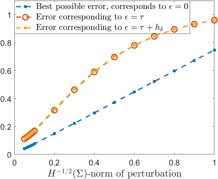
Refer to caption
Refer to caption
Figure 2. Poisson’s equation. Norm of perturbation vs. relative L2​(Ω)L_{2}(\Omega)-error in case of randomly perturbed Neumann data for different choices of ε\varepsilon. Left: Random perturbations of varying H−1/2(Σ)H^{-1/2}(\Sigma)-norm and fixed mesh with #​DoFs≈105\#\mbox{DoFs}\approx 10^{5}. Right: Random perturbations with H−1/2(Σ)H^{-1/2}(\Sigma)-norm equal to 0.1, and varying mesh-size.

We conclude that, for this problem, apparently such random perturbations are harmless, because without any regularization, for hδ↓0h_{\delta}\downarrow 0, which results in an increasingly ill-posed problem, their effect on the error hardly increases.

8.1.3. ‘Difficult’ perturbations

From [ARRV09] we know that for m∈ℕm\in\mathbb{N}, the solution u=u(m)u=u^{(m)} of the Cauchy problem (8.1) with data f=f(m)=(0,0,fN(m))f=f^{(m)}=(0,0,f_{N}^{(m)}) where fN(m)​(x):=−2​mπ​sin⁡m​xf_{N}^{(m)}(x):=-\sqrt{\frac{2m}{\pi}}\sin mx, is given by u(m)​(x,y)=2m​π​sin⁡m​x​sinh⁡m​yu^{(m)}(x,y)=\sqrt{\frac{2}{m\pi}}\sin mx\sinh my. It holds that ‖fN(m)‖H−12​(Σ)=1\|f_{N}^{(m)}\|_{H^{-\frac{1}{2}}(\Sigma)}=1, ‖u(m)‖H1​(Ω)≂|u(m)|H1​(Ω)=12​sinh⁡2​m∼12​em\|u^{(m)}\|_{H^{1}(\Omega)}\eqsim|u^{(m)}|_{H^{1}(\Omega)}=\sqrt{\frac{1}{2}\sinh 2m}\sim\frac{1}{2}e^{m} (m→∞m\rightarrow\infty), and ‖u(m)‖L2​(Ω)∼em2​2​m\|u^{(m)}\|_{L_{2}(\Omega)}\sim\frac{e^{m}}{2\sqrt{2}m} (m→∞m\rightarrow\infty), illustrating the strong ill-posedness of the Cauchy problem.

We investigate our numerical solver when we perturb the exact Neumann datum from (8.2) with 0.1∗f(m)0.1*f^{(m)}. We compare the same regularization strategies as with random perturbations. The results given in Figure 3 show that both for m=1,3m=1,3 as well as for m=16m=16 regularization at most slightly improves the results. For m=1,3m=1,3 this can be understood because the perturbation has an only modest effect on the solution. An explanation why for m=16m=16 regularization is hardly helpful is that on the meshes that we employed apparently the best representation of u(16)u^{(16)} has a much smaller norm than u(16)u^{(16)} itself. For the intermediate value m=6m=6, however, we clearly see that regularization is helpful.

Refer to caption
(a) For m=1m=1.
Refer to caption
(b) For m=3m=3.
Refer to caption
(c) For m=6m=6.
Refer to caption
(d) For m=16m=16.
Figure 3. Poisson’s equation. Meshsize vs. relative L2​(Ω)L_{2}(\Omega)-error for different choices of ε\varepsilon and perturbation with 0.1​2​mπ​sin⁡m​x0.1\sqrt{\frac{2m}{\pi}}\sin mx of the Neumann datum for m=1,3,6,16m=1,3,6,16.

8.2. Data-assimilation for the wave equation

For Ω=(0,1)\Omega=(0,1), I=(0,1)I=(0,1) and ω=(12,34)\omega=(\tfrac{1}{2},\tfrac{3}{4}), given (f,g,h)∈H−1​(I×Ω)×L2​(I×∂Ω)×L2​(I×ω)(f,g,h)\in H^{-1}(I\times\Omega)\times L_{2}(I\times\partial\Omega)\times L_{2}(I\times\omega), we consider the problem of finding uu that solves

∂2u∂t2−△x​u=f​ on ​I×Ω,u=g​ on ​I×∂Ω,u=h​ on ​I×ω,\frac{\partial^{2}u}{\partial t^{2}}-\triangle_{x}u=f\text{ on }I\times\Omega,\quad u=g\text{ on }I\times\partial\Omega,\quad u=h\text{ on }I\times\omega,

or, more precisely its variational formulation A​u=(f,g,h)Au=(f,g,h) with A:=(□,γI×∂Ω,ΓI×ω)A:=(\Box,\gamma_{I\times\partial\Omega},\Gamma_{I\times\omega}) given in Example 3.3.

We consider a sequence of uniform triangulations (𝒯δ)δ∈Δ({\mathcal{T}}^{\delta})_{\delta\in\Delta} of I×Ω¯\overline{I\times\Omega}, where each next triangulation is created from its predecessor by one uniform newest vertex bisection starting from an initial triangulation that is created by cutting I×ΩI\times\Omega along both diagonals. The interior vertex in this initial triangulation is labelled as the ‘newest vertex’ of all four triangles.

Following Sect. 7.4, we take Xδ:=𝒮𝒯δ0,1​(I×Ω)X^{\delta}:=\mathcal{S}_{{\mathcal{T}}^{\delta}}^{0,1}(I\times\Omega), and with 𝒯sδ{\mathcal{T}}^{\delta}_{s} denoting the second successor of 𝒯δ{\mathcal{T}}^{\delta} in the sequence of triangulations, we set Yδ:=𝒮𝒯sδ0,1∩H01​(I×Ω)Y^{\delta}:=\mathcal{S}^{0,1}_{{\mathcal{T}}_{s}^{\delta}}\cap H^{1}_{0}(I\times\Omega).

Considering the unconditional stability estimate  (3.3) in Example 3.3, our approach is to minimize the least squares functional ‖□​z−f‖H−1​(I×Ω)2+‖γI×∂Ω​z−g‖L2​(I×∂Ω)2+‖ΓI×ω​z−h‖L2​(I×ω)2\|\Box z-f\|_{H^{-1}(I\times\Omega)}^{2}+\|\gamma_{I\times\partial\Omega}z-g\|_{L_{2}(I\times\partial\Omega)}^{2}+\|\Gamma_{I\times\omega}z-h\|_{L_{2}(I\times\omega)}^{2} over z∈Xδz\in X^{\delta}, so without regularization term. To make this method feasible without comprimizing its qualitative properties, first we replace the supremum from the first term by the supremum over YδY^{\delta} (see Proposition 7.11). Second, to make the computation of the resulting dual norm efficient, we introduce a preconditioner GYδ∈ℒ​is​(Yδ′,Yδ)G_{Y}^{\delta}\in\mathcal{L}\mathrm{is}({Y^{\delta}}^{\prime},Y^{\delta}) with ‖GYδ​f‖H1​(Ω)2≂f⁡(GYδ​f)\|G_{Y}^{\delta}f\|_{H^{1}(\Omega)}^{2}\eqsim f(G_{Y}^{\delta}f) (f∈Yδ′f\in{Y^{\delta}}^{\prime}), and compute our approximation uδu^{\delta} as the unique solution in XδX^{\delta} of the symmetric positive definite system

(□​uδ−f)​(GYδ​□​z~)\displaystyle(\Box u^{\delta}-f)(G_{Y}^{\delta}\Box\tilde{z}) +⟨γI×∂Ω​uδ−g,γI×∂Ω​z~⟩L2​(I×∂Ω)\displaystyle+\langle\gamma_{I\times\partial\Omega}u^{\delta}-g,\gamma_{I\times\partial\Omega}\tilde{z}\rangle_{L_{2}(I\times\partial\Omega)}
+⟨ΓI×ω​uδ−h,ΓI×ω​z~⟩L2​(I×ω)=0​(z~∈Xδ).\displaystyle+\langle\Gamma_{I\times\omega}u^{\delta}-h,\Gamma_{I\times\omega}\tilde{z}\rangle_{L_{2}(I\times\omega)}=0\,\,\,\,(\tilde{z}\in X^{\delta}).

For GYδG_{Y}^{\delta} we use a common (multiplicative) multi-level preconditioner.

In our experiments, we prescribe the solution

u⁡(t,x)=cos⁡(π​t)​sin⁡(π​x),u(t,x)=\cos(\pi t)\sin(\pi x),

which corresponds to (exact) data

(f,g,h)=(0,0,u|I×ω).(f,g,h)=\big(0,0,u|_{I\times\omega}\big).

We perform experiments with unperturbed and perturbed data. Instead of the error in the hard to evaluate norm ∥⋅∥L∞​(I,L2​(Ω))+∥∂t⋅∥L2​(I,H−1​(Ω))\|\cdot\|_{L_{\infty}(I;L_{2}(\Omega))}+\|\partial_{t}\cdot\|_{L_{2}(I;H^{-1}(\Omega))} from the unconditional stability estimate (3.3), we provide the a posteriori residual estimator from Section 6 given by

(f−□​uδ)​(GYδ​(f−□​uεδ)+‖γI×∂Ω​uεδ−g‖L2​(I×∂Ω)2+‖ΓI×ω​uεδ−h‖L2​(I×ω)2CLOSE,\sqrt{(f-\Box u^{\delta})(G_{Y}^{\delta}(f-\Box u_{\varepsilon}^{\delta})+\|\gamma_{I\times\partial\Omega}u_{\varepsilon}^{\delta}-g\|_{L_{2}(I\times\partial\Omega)}^{2}+\|\Gamma_{I\times\omega}u_{\varepsilon}^{\delta}-h\|_{L_{2}(I\times\omega)}^{2}},

which provides, modulo a constant factor, an upper bound for the aforementioned norm of the error up to data oscillations. We additionally provide the relative errors in the easily evaluable L2​(I×Ω)L_{2}(I\times\Omega)- and H1​(I×Ω)H^{1}(I\times\Omega)-norms (i.e., these norms divided by the corresponding norm of the exact solution).

For the perturbed case we add to hh either a constant perturbation with L2​(I×ω)L_{2}(I\times\omega)-norm equal to τ\tau, or a random perturbation of the form p=τ​p^‖p^‖L2​(I×ω)p=\tau\frac{\hat{p}}{\|\hat{p}\|_{L_{2}(I\times\omega)}}, where p^\hat{p} is a random function in XδX^{\delta} with values in [0,1][0,1]. We take τ=0.01\tau=0.01. Figure 4 shows the numerical results.

Refer to caption
(a) Unperturbed data.
Refer to caption
(b) Perturbations, with L2​(I×ω)L_{2}(I\times\omega)-norm equal to 0.010.01, of datum hh.
Figure 4. Data assimilation for the wave equation. Meshsize vs. relative error (or residual estimator).

In the unperturbed cases, the rates for L2​(I×Ω)L_{2}(I\times\Omega)- and H1​(I×Ω)H^{1}(I\times\Omega)-norms are equal to the best approximation rates in these norms.

8.3. Data-assimilation for the heat equation

For Ω=(0,1)d\Omega=(0,1)^{d}, I=(0,1)I=(0,1) and ω=(14,34)d\omega=(\frac{1}{4},\frac{3}{4})^{d}, given (f,g)∈L2​(I,H−1​(Ω))×L2​(I×ω)(f,g)\in L_{2}(I;H^{-1}(\Omega))\times L_{2}(I\times\omega), we consider the problem of finding uu that solves the problem

∂tu−△x​u=f​ on ​I×Ω,u|I×ω=g,\partial_{t}u-\triangle_{x}u=f\text{ on }I\times\Omega,\quad u|_{I\times\omega}=g,

which was discussed in Example 3.2. We consider the formulation of this problem as a first order system as analyzed in Sect. 7.3. Assuming f∈L2​(I×Ω)f\in L_{2}(I\times\Omega), for 𝐮=(u1,𝐮2)=(u,−∇xu){\bf u}=(u_{1},{\bf u}_{2})=(u,-\nabla_{x}u), it reads as A~​𝐮:=(𝐮2+∇xu1,div⁡𝐮,ΓI×ω​u1)=(0,f,g)\widetilde{A}{\bf u}:=({\bf u}_{2}+\nabla_{x}u_{1},\divv{\bf u},\Gamma_{I\times\omega}u_{1})=(0,f,g), where div⁡𝐮:=∂tu1+divx⁡𝐮2\divv{\bf u}:=\partial_{t}u_{1}+\divv_{x}{\bf u}_{2} and 𝐮∈X~:={𝐮=(u1,𝐮2)∈L2​(I,H1​(Ω))×L2​(I×Ω)d:div⁡𝐮∈L2​(I×Ω)}{\bf u}\in\widetilde{X}:=\big\{{\bf u}=(u_{1},{\bf u}_{2})\in L_{2}(I;H^{1}(\Omega))\times L_{2}(I\times\Omega)^{d}\colon\divv{\bf u}\in L_{2}(I\times\Omega)\big\}. Recall that we study this problem in two cases. Either we have no knowledge of uu on I×∂ΩI\times\partial\Omega (Case  (a)), or uu is required to vanish on this lateral boundary (Case  (b)). The latter problem is unconditionally stable. In this Case  (b), the space L2​(I,H1​(Ω))L_{2}(I;H^{1}(\Omega)) should be read as L2​(I,H01​(Ω))L_{2}(I;H_{0}^{1}(\Omega)).

In view of the conditional or unconditional stability estimates (7.5) or (7.6), respectively, given a finite dimensional subspace Xδ⊂X~X^{\delta}\subset\widetilde{X}, with V~:=L2​(I×Ω)d×L2​(I×Ω)×L2​(I×ω)\widetilde{V}:=L_{2}(I\times\Omega)^{d}\times L_{2}(I\times\Omega)\times L_{2}(I\times\omega) our approach is to minimize the least squares functional ‖A~​𝐮−(0,f,g)‖V~2+ε2​‖u1‖L2​(I×Ω)2\|\widetilde{A}{\bf u}-(0,f,g)\|_{\widetilde{V}}^{2}+\varepsilon^{2}\|u_{1}\|_{L_{2}(I\times\Omega)}^{2} over 𝐮∈Xδ{\bf u}\in X^{\delta}, where in Case (b) the regularization term ε2​‖u1‖L2​(I×Ω)2\varepsilon^{2}\|u_{1}\|_{L_{2}(I\times\Omega)}^{2} is omitted.

In our experiments, we prescribe the solution

u⁡(t,x)=(t3+1)​∏i=1dsin⁡(π​xi),u(t,x)=(t^{3}+1)\prod_{i=1}^{d}\sin(\pi x_{i}),

and define the data (f,g)(f,g) correspondingly. For Case (a) the errors are measured in the relative L2​((T1,T2),H1​(ω˘))L_{2}((T_{1},T_{2});H^{1}(\breve{\omega}))-norm, where we take T1=18T_{1}=\frac{1}{8}, T2=78T_{2}=\frac{7}{8} and ω˘=(18,78)d\breve{\omega}=(\frac{1}{8},\frac{7}{8})^{d}. Instead of recording the error in the L2​((T1,T),H01​(Ω))∩H1​((T1,T),H−1​(Ω))L_{2}((T_{1},T);H^{1}_{0}(\Omega))\cap H^{1}((T_{1},T);H^{-1}(\Omega))-norm, which is hard to evaluate, we make use of the unconditional stability estimate (7.6) for Case (b), and provide the residual ‖A~​𝐮−(0,f,g)‖V~\|\widetilde{A}{\bf u}-(0,f,g)\|_{\widetilde{V}} which, modulo a constant factor, is an upper bound for the aforementioned norm of the error. In addition we measure relative errors in the L2​((T1,T),H1​(Ω))L_{2}((T_{1},T);H^{1}(\Omega))-norm for T1=18T_{1}=\frac{1}{8} which is easy to evaluate.

8.3.1. Unperturbed data, and Ω=(0,1)\Omega=(0,1)

We consider a sequence of uniform triangulations (𝒯δ)δ∈Δ({\mathcal{T}}^{\delta})_{\delta\in\Delta} of I×Ω¯\overline{I\times\Omega}, where each next triangulation is created from its predecessor by one uniform newest vertex bisection starting from an initial triangulation that is created by cutting I×ΩI\times\Omega along both diagonals. The interior vertex in this initial triangulation is labelled as the ‘newest vertex’ of all four triangles. We set Xδ:=𝒮𝒯δ0,1​(I×Ω)×𝒮𝒯δ0,1​(I×Ω)dX^{\delta}:=\mathcal{S}_{{\mathcal{T}}^{\delta}}^{0,1}(I\times\Omega)\times\mathcal{S}_{{\mathcal{T}}^{\delta}}^{0,1}(I\times\Omega)^{d} in Case (a), and Xδ:=(𝒮𝒯δ0,1​(I×Ω)∩L2​(I,H01​(Ω)))×𝒮𝒯δ0,1​(I×Ω)dX^{\delta}:=(\mathcal{S}_{{\mathcal{T}}^{\delta}}^{0,1}(I\times\Omega)\cap L_{2}(I;H_{0}^{1}(\Omega)))\times\mathcal{S}_{{\mathcal{T}}^{\delta}}^{0,1}(I\times\Omega)^{d} in Case (b).

Taking unperturbed data, we consider two strategies for choosing the regularization parameter ε\varepsilon in Case (a), namely ε=0\varepsilon=0 and ε=hδ\varepsilon=h_{\delta}, the latter being the mesh-size. Since uu is smooth, the choice ε=hδ\varepsilon=h_{\delta} satisfies the conditions in (2.5). In Figure 5, we give the relative errors for both these choices of ε\varepsilon, and also give the relative error and residual estimator in Case (b). In the latter unconditionally stable case no regularization is applied.

As in the case of the Cauchy problem for Poisson’s equation, the numerical results in Figure 5 indicate that with unperturbed data regularization is not helpful. The rates for L2​((18,78),H1​((18,78)d))L_{2}((\frac{1}{8},\frac{7}{8});H^{1}((\frac{1}{8},\frac{7}{8})^{d}))- or L2​((18,1),H1​(0,1))L_{2}((\frac{1}{8},1);H^{1}(0,1))-norms are equal to the best approximation rates in these norms.

Refer to caption
Figure 5. Data assimilation for the heat equation, and Ω=(0,1)\Omega=(0,1). Meshsize vs. relative error (or residual estimator) in case of unperturbed data. Note that the norms in which the errors are measured are different for Case (a) and Case (b). The asymptotic convergence rate in terms of #\# DoFs, indicated by the solid straight lines, is 0.50.5.

8.3.2. Randomly perturbed data, Ω=(0,1)\Omega=(0,1)

For (Xδ)δ∈Δ(X^{\delta})_{\delta\in\Delta} as in Sect. 8.3.1, we now perturb the observational datum gg with a random piecewise constant p∈𝒮𝒯δ−1,0p\in\mathcal{S}^{-1,0}_{\mathcal{T}^{\delta}} with ‖p‖L2​(ω)=τ||p||_{L_{2}(\omega)}=\tau. This pp is constructed by normalizing a random function p^∈𝒮𝒯δ−1,0\hat{p}\in\mathcal{S}^{-1,0}_{\mathcal{T}^{\delta}} and multiplying with τ\tau. We considered the cases where p^\hat{p} takes values in either [0,1][0,1] or [−12,12][-\frac{1}{2},\frac{1}{2}].

For Case (a), we compare the results obtained with the regularization strategies ε=τ\varepsilon=\tau, and ε=τ+hδ\varepsilon=\tau+h_{\delta}, where the latter choice satisfies the conditions in (2.5), with those obtained with the experimentally found ε\varepsilon that minimizes ‖u−uεδ‖L2​(I,H1​(Ω))||u-u_{\varepsilon}^{\delta}||_{L_{2}(I;H^{1}(\Omega))}. In addition, we present the results obtained for Case (b). The results are shown in Figure 6.

Refer to caption
Refer to caption
Figure 6. Data assimilation for the heat equation, and Ω=(0,1)\Omega=(0,1). Norm of perturbation vs. relative error (or residual estimator). Results for random perturbation of the observational datum gg, for a fixed mesh with #\# DoFs ≈106\approx 10^{6} for different choices of ε\varepsilon and τ\tau. Left: the case where p^\hat{p} takes values in [0,1][0,1]. Right: the case where p^\hat{p} takes values in [−1/2,1/2][-1/2,1/2].

For both Case (a) and (b), the solution is much more sensitive to random perturbations with mean τ/2\tau/2 than to those with mean 00. In Case (a) regularization is helpful for perturbations with mean τ/2\tau/2, but it is not when the mean is 00.

8.3.3. Unperturbed data, and Ω=(0,1)2\Omega=(0,1)^{2}

We now consider the data-assimilation problem described in Sect. 8.3 for unperturbed data and the two-dimensional spatial domain Ω=(0,1)2\Omega=(0,1)^{2}. We consider a sequence of conforming partitions (𝒯δ)δ∈Δ({\mathcal{T}}^{\delta})_{\delta\in\Delta} of I×Ω¯\overline{I\times\Omega} into tetrahedra, where each partition consists of hδ−3h_{\delta}^{-3} cubes with sidelength hδh_{\delta} that are decomposed into 6 tetrahedra using the Kuhn splitting. Since with our mesh-sizes and linear finite elements we could not clearly observe convergence in Case (a), we take quadratic elements, i.e., we set Xδ:=𝒮𝒯δ0,2​(I×Ω)×𝒮𝒯δ0,2​(I×Ω)2X^{\delta}:=\mathcal{S}_{{\mathcal{T}}^{\delta}}^{0,2}(I\times\Omega)\times\mathcal{S}_{{\mathcal{T}}^{\delta}}^{0,2}(I\times\Omega)^{2} in Case (a), and Xδ:=(𝒮𝒯δ0,2​(I×Ω)∩L2​(I,H01​(Ω)))×𝒮𝒯δ0,2​(I×Ω)2X^{\delta}:=(\mathcal{S}_{{\mathcal{T}}^{\delta}}^{0,2}(I\times\Omega)\cap L_{2}(I;H_{0}^{1}(\Omega)))\times\mathcal{S}_{{\mathcal{T}}^{\delta}}^{0,2}(I\times\Omega)^{2} in Case (b).

We consider regularization parameters ε=0\varepsilon=0 and ε=hδ2\varepsilon=h_{\delta}^{2} for Case (a), where the latter satisfies the conditions in (2.5), and for Case (b) apply no regularization. The results are given in Figure 7.

Refer to caption
Figure 7. Data assimilation for the heat equation, and Ω=(0,1)2\Omega=(0,1)^{2}. Meshsize vs. relative error (or residual estimator) in case of unperturbed data. The asymptotic convergence rate in terms of #\# DoFs indicated by the dashed straight lines is 11.

9. Conclusion

We have constructed a least squares solver for general conditionally stable ill-posed PDEs. For this solver it was demonstrated that, for a suitable regularization parameter, the error in the numerical approximation is qualitatively the best that can be expected in view of the conditional stability estimate. In applications the least squares functional to be minimized involves negative and/or fractional Sobolev norms of residuals. It was shown that these norms can be replaced by computable quantities without compromizing any of the attractive theoretical properties of the method.

The theoretical results were illustrated by numerical experiments for Poisson’s equation with Cauchy data, and data-assimilation problems for both heat and wave-equation. In several examples the bounds on the error in the numerical approximation that were derived using the conditional stability estimates were pessimistic, which is not surprising since these estimates cover worst case settings. Similarly, it turns out that in many cases better results were obtained by applying a smaller regularization parameter than predicted by the theoretical estimates.

References

  • [AL09] M. Arioli and D. Loghin. Discrete interpolation norms with applications. SIAM J. Numer. Anal., 47(4):2924–2951, 2009. doi:10.1137/080729360.
  • [ARRV09] G. Alessandrini, L. Rondi, E. Rosset, and S. Vessella. The stability for the Cauchy problem for elliptic equations. Inverse Problems, 25(12):123004, 47, 2009. doi:10.1088/0266-5611/25/12/123004.
  • [Bar70] C. Bardos. Problèmes aux limites pour les équations aux dérivées partielles du premier ordre à coefficients réels; théorèmes d’approximation; application à l’équation de transport. Ann. Sci. École Norm. Sup. (4), 3:185–233, 1970.
  • [BBFD15] El. Bécache, L. Bourgeois, L. Franceschini, and J. Dardé. Application of mixed formulations of quasi-reversibility to solve ill-posed problems for heat and wave equations: the 1D case. Inverse Probl. Imaging, 9(4):971–1002, 2015. doi:10.3934/ipi.2015.9.971.
  • [BC20] L. Bourgeois and L. Chesnel. On quasi-reversibility solutions to the Cauchy problem for the Laplace equation: regularity and error estimates. ESAIM Math. Model. Numer. Anal., 54(2):493–529, 2020. doi:10.1051/m2an/2019073.
  • [BDE22] E. Burman, G. Delay, and A. Ern. The unique continuation problem for the heat equation discretized with a high-order space-time nonconforming method. hal 03720960, 2022.
  • [BFMO21a] E. Burman, A. Feizmohammadi, A. Münch, and L. Oksanen. Space time stabilized finite element methods for a unique continuation problem subject to the wave equation. ESAIM Math. Model. Numer. Anal., 55(suppl.):S969–S991, 2021. doi:10.1051/m2an/2020062.
  • [BFMO21b] E. Burman, A. Feizmohammadi, A. Münch, and L. Oksanen. Spacetime finite element methods for control problems subject to the wave equation, 2021. arXiv:2109.07890.
  • [BFO20] E. Burman, A. Feizmohammadi, and L. Oksanen. A finite element data assimilation method for the wave equation. Math. Comp., 89(324):1681–1709, 2020. doi:10.1090/mcom/3508.
  • [BG09] P. B. Bochev and M. D. Gunzburger. Least-squares finite element methods, volume 166 of Applied Mathematical Sciences. Springer, New York, 2009. doi:10.1007/b13382.
  • [BHL18] E. Burman, P. Hansbo, and M.G. Larson. Solving ill-posed control problems by stabilized finite element methods: an alternative to Tikhonov regularization. Inverse Problems, 34(3):035004, 36, 2018. doi:10.1088/1361-6420/aaa32b.
  • [BIHO18] E. Burman, J. Ish-Horowicz, and L. Oksanen. Fully discrete finite element data assimilation method for the heat equation. ESAIM Math. Model. Numer. Anal., 52(5):2065–2082, 2018. doi:10.1051/m2an/2018030.
  • [BLR92] C. Bardos, G. Lebeau, and J. Rauch. Sharp sufficient conditions for the observation, control, and stabilization of waves from the boundary. SIAM J. Control Optim., 30(5):1024–1065, 1992. doi:10.1137/0330055.
  • [BO18] E. Burman and L. Oksanen. Data assimilation for the heat equation using stabilized finite element methods. Numer. Math., 139(3):505–528, 2018. doi:10.1007/s00211-018-0949-3.
  • [BPX90] J.H. Bramble, J.E. Pasciak, and J. Xu. Parallel multilevel preconditioners. Math. Comp., 55:1–22, 1990.
  • [BR85] C. Bernardi and G. Raugel. Analysis of some finite elements for the Stokes problem. Math. Comp., 44(169):71–79, 1985. doi:10.2307/2007793.
  • [BR18] L. Bourgeois and A. Recoquillay. A mixed formulation of the Tikhonov regularization and its application to inverse PDE problems. ESAIM Math. Model. Numer. Anal., 52(1):123–145, 2018. doi:10.1051/m2an/2018008.
  • [Bur98] N. Burq. Contrôle de l’équation des ondes dans des ouverts comportant des coins. Bull. Soc. Math. France, 126(4):601–637, 1998. Appendix B written in collaboration with Jean-Marc Schlenker. URL: http://www.numdam.org/item?id=BSMF_1998__126_4_601_0.
  • [Bur16] E. Burman. Stabilised finite element methods for ill-posed problems with conditional stability. In Building bridges: connections and challenges in modern approaches to numerical partial differential equations, volume 114 of Lect. Notes Comput. Sci. Eng., pages 93–127. Springer, [Cham], 2016.
  • [Bur17] E. Burman. The elliptic Cauchy problem revisited: control of boundary data in natural norms. C. R. Math. Acad. Sci. Paris, 355(4):479–484, 2017. doi:10.1016/j.crma.2017.02.014.
  • [DSW22] W. Dahmen, R. Stevenson, and J. Westerdiep. Accuracy controlled data assimilation for parabolic problems. Math. Comp., 91(334):557–595, 2022. doi:10.1090/mcom/3680.
  • [Füh21] Th. Führer. Multilevel decompositions and norms for negative order Sobolev spaces. Math. Comp., 91(333):183–218, 2021. doi:10.1090/mcom/3674.
  • [FK21] Th. Führer and M. Karkulik. Space-time least-squares finite elements for parabolic equations. Comput. Math. Appl., 92:27–36, 2021. doi:10.1016/j.camwa.2021.03.004.
  • [FPW11] S. Funken, D. Praetorius, and P. Wissgott. Efficient implementation of adaptive P1-FEM in Matlab. Comput. Methods Appl. Math., 11(4):460–490, 2011. doi:10.2478/cmam-2011-0026.
  • [GS21] G. Gantner and R.P. Stevenson. Further results on a space-time FOSLS formulation of parabolic PDEs. ESAIM Math. Model. Numer. Anal., 55(1):283–299, 2021. doi:10.1051/m2an/2020084.
  • [Isa06] V. Isakov. Inverse problems for partial differential equations, volume 127 of Applied Mathematical Sciences. Springer, New York, second edition, 2006.
  • [IY14] O. Imanuvilov and M. Yamamoto. Conditional stability in a backward parabolic system. Appl. Anal., 93(10):2174–2198, 2014. doi:10.1080/00036811.2013.873412.
  • [Kli06] M.V. Klibanov. Estimates of initial conditions of parabolic equations and inequalities via lateral Cauchy data. Inverse Problems, 22(2):495–514, 2006. doi:10.1088/0266-5611/22/2/007.
  • [LLT86] I. Lasiecka, J.-L. Lions, and R. Triggiani. Nonhomogeneous boundary value problems for second order hyperbolic operators. J. Math. Pures Appl. (9), 65(2):149–192, 1986.
  • [LM72] J.-L. Lions and E. Magenes. Non-homogeneous boundary value problems and applications. Vol. I. Springer-Verlag, New York-Heidelberg, 1972. Translated from the French by P. Kenneth, Die Grundlehren der mathematischen Wissenschaften, Band 181.
  • [LRLTT17] J. Le Rousseau, G. Lebeau, P. Terpolilli, and E. Trélat. Geometric control condition for the wave equation with a time-dependent observation domain. Anal. PDE, 10(4):983–1015, 2017. doi:10.2140/apde.2017.10.983.
  • [PP13] M. Page and D. Praetorius. Convergence of adaptive FEM for some elliptic obstacle problem. Appl. Anal., 92(3):595–615, 2013. doi:10.1080/00036811.2011.631916.
  • [Sch14] J. Schöberl. C++11 implementation of finite elements in ngsolve. Technical report, Institute for Analysis and Scientific Computing. Vienna University of Technology, 2014.
  • [SvV20a] R.P. Stevenson and R. van Venetië. Uniform preconditioners for problems of negative order. Math. Comp., 89(322):645–674, 2020. doi:10.1090/mcom/3481.
  • [SvV20b] R.P. Stevenson and R. van Venetië. Uniform preconditioners for problems of positive order. Comput. Math. Appl., 79(12):3516–3530, 2020. doi:10.1016/j.camwa.2020.02.009.
  • [SvV21] R.P. Stevenson and R. van Venetië. Uniform Preconditioners of Linear Complexity for Problems of Negative Order. Comput. Methods Appl. Math., 21(2):469–478, 2021. doi:10.1515/cmam-2020-0052.
  • [SW21a] R.P. Stevenson and J. Westerdiep. Minimal residual space-time discretizations of parabolic equations: asymmetric spatial operators. Comput. Math. Appl., 101:107–118, 2021. doi:10.1016/j.camwa.2021.09.014.
  • [SW21b] R.P. Stevenson and J. Westerdiep. Stability of Galerkin discretizations of a mixed space-time variational formulation of parabolic evolution equations. IMA J. Numer. Anal., 41(1):28–47, 2021. doi:10.1093/imanum/drz069.
  • [SZ90] L. R. Scott and S. Zhang. Finite element interpolation of nonsmooth functions satisfying boundary conditions. Math. Comp., 54(190):483–493, 1990.
  • [Tik43] A. N. Tikhonov. On the stability of inverse problems. C. R. (Doklady) Acad. Sci. URSS (N.S.), 39:176–179, 1943.