Transverse-momentum-dependent wave functions and Soft functions at one-loop in Large Momentum Effective Theory

The exploration of underlying structures of hadrons has always been one of the most important frontiers in particle and nuclear physics. The one-dimensional and three-dimensional light-front wave functions (LFWFs) are important physical quantities describing the distributions of constituents’ momentum in the hadron, and reflect the non-perturbative internal structure of hadrons Lepage:1979zb; Lepage:1980fj; Brodsky:1997de. As for a light Nambu-Goldstone boson, the LFWFs also help us to understand the chiral symmetry breaking Politzer:1982mf; Miransky:1985wzx; Alkofer:2008tt; Serna:2018dwk.

It was firstly noticed that in an exclusive process Lepage:1979zb; Lepage:1980fj the non-perturbative LFWFs for a given Fock state are required. As an inevitable input, LFWFs also play an important role in theoretical analyses of $B$ meson weak decays Li:1994iu; Keum:2000wi; Keum:2000ph; Lu:2000em; Beneke:2001ev, which are of great values for the test of the standard model (SM) and the search for new physics beyond the SM. The unprecedented high precision of measurements at the current and forthcoming experimental facilities strongly request the improvement of the accuracy of these non-perturbative physical quantities from quantum chromodynamics (QCD).

In 1970s, the formation of one-dimensional hadronic wave function, namely, light-cone distribution amplitudes (LCDAs) was established in the large momentum limit under light-front quantization Lepage:1979zb. Results for a few lowest moments of the LCDAs were firstly obtained from QCD sum rules Shifman:1978bx; Chernyak:1983ej, and since then many progresses have been made in extracting the moments of LCDAs in the past decades. Despite of these progresses, a complete knowledge of meson wave functions from the first principle is not well-established yet.

An obvious difficulty in calculating LCDAs lies in the fact that it is inherently non-perturbative and needs to be treated by methods such as lattice QCD (LQCD). However, LCDAs belong to light-cone correlations of quark/gluon field operators, and thus contain explicit time dependence, which cannot be directly calculated by lattice field theory defined in the Euclidean spacetime. In this respect, only the moments of LCDAs, namely matrix elements of the local operators, can be performed in the traditional LQCD approach Gockeler:2005jz; Braun:2006dg; Boyle:2006pw; Arthur:2010xf; Braun:2015axa; Bali:2017ude; RQCD:2019osh.

A remarkable approach to circumvent the above problem is proposed in Ref. Ji:2013dva; Ji:2014gla, which is now systematically formulated as large momentum effective theory (LaMET). In LaMET, one can construct the directly computable hadron matrix elements with non-local operators, named as quasi-distributions, on the lattice. Through a perturbative matching, the corresponding LCDAs can be accessed Ji:2013dva; Ji:2014gla; Cichy:2018mum; Ji:2020ect. Many inspiring results on LCDAs were reported in recent years, and reviews of recent developments can be found in Refs. Cichy:2018mum; Ji:2020ect.

Compared with LCDAs and parton distribution functions (PDFs), transverse-momentum-dependent wave functions (TMDWFs) and TMD parton distribution functions (TMDPDFs) provide more versatile information on the internal three-dimensional structure of hadrons, which are also relevant for observables with transverse momentum dependent (TMD) distributions of final-state particles in high-energy experiments. For instance, TMDWFs have been applied to calculate various transition form factors such as the pion electromagnetic form factor Li:1992nu; Efremov:1979qk, the proton form factors  Aznaurian:1979zz; Li:1992ce; Duncan:1979hi; Lepage:1979za and exclusive $B$ decays Li:1994iu; Li:2012nk. Therefore, it is highly prerequisite to further investigate the three-dimensional LFWFs from the first-principle QCD.

A very important progress in LaMET is that TMD distributions can be accessible through the Euclidean equal-time correlations Ebert:2019okf; Ebert:2019tvc; Ji:2019sxk; Ji:2019ewn; Ji:2021znw. In Ref. Ji:2019sxk, it has been demonstrated that the form factor of a bi-local four-quark operator, calculable on the lattice, can be factorized into TMDWFs, a universal soft factor (function) and the matching kernel through QCD factorization at large momentum transfer. A combined analysis of quasi-TMDWFs on lattice allows a direct extraction of the universal soft function and TMDWFs. Based on these proposals, Lattice determinations of the rapidity evolution anomalous dimension, namely Collins-Soper (CS) kernel Collins:1981va, can be found in Refs. Shanahan:2020zxr; LatticeParton:2020uhz; Schlemmer:2021aij; Li:2021wvl; Shanahan:2021tst; LPC:2022ibr.

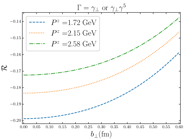
It is anticipated that in the large momentum limit, the form factor can be expressed as a convolution of TMDWFs, soft functions and a hard kernel. In this work, we aim to present a complete one-loop analysis of these quantities and provide the necessary details to the proposal in Refs. Ji:2019sxk; Ji:2021znw. We use the expansion by regions and provide a proof of the TMD factorization for the form factor. In the explicit calculation factor, we adopt a modern technique based on the integration by part (IBP). With these results, we will demonstrate the cancellation of the infrared divergences, and explicitly validate the TMD factorization. Finally, we extract the hard kernels for the form factor and quasi-TMDWFs through the factorization, which will be useful for a precision determination of TMDWFs and soft functions. We also make use of the lattice data from Lattice Parton Collaboration on quasi-TMDWFs LPC:2022ibr and show that the perturbative corrections to soft functions depend on the Lorentz structures, and the magnitude can reach the order $(10-30)\%$. The results are found to be less sensitive to the transverse separation, which may imply a factorized form for the quasi-TMDWFs. As a comparison, we also give a phenomenological parametrization which contains explicit dependence on the transverse separation.

The rest of this work is organized as follows. In Sec. II we will briefly introduce the concept of TMDWFs. In Sec. III, the one-loop perturbative results for TMDWFs, soft functions, form factors and Wilson loops will be presented in order. To regularize the rapidity divergence in TMDWFs and soft function, the delta regulator will be used in the calculation. Based on these results, we will explicitly validate the TMD factorization of four quark form factors and extract the short-distance hard kernel at one-loop level. In Sec.  IV, the one-loop perturbative results for quasi-TMDWFs will be presented. In Sec. V, we use the hard kernel and calculate the effects to extract the soft functions. We conclude this work in Sec. VI. In the appendix, we collect some details in the calculation.

In this section, we will follow the spirit of Ref. Ji:2021znw and give a self-contained description of TMDWFs.

An intuitive identification of LFWFs is the light front correlation functions between hadron state and QCD vacuum, in which light-like gauge links extending to infinities are required to maintain the gauge invariance. This allows the identification of LF divergences as rapidity divergences, known in the literature of TMD physics.

In high energy limit, light quarks and gluons inside a hadron move on the lightcone, and are generally named as partons. In parton physics, light-front quantization (LFQ) is a useful formalism to handle the hadron states. It provides a Hamiltonian description of QCD similar with the diagonalized Hamiltonian in non-relativistic quantum mechanics as

where $|\Psi_{n}\rangle$ denotes a QCD bound state Brodsky:1997de, and $P^{+}=(P^{0}+P^{z})/\sqrt{2}$. The wave functions obtained in this picture can in principle be used to calculate all partonic densities and correlations functions.

In the infinity momentum frame (IMF), making an IR cut-off on the longitudinal momentum scale $k^{+}=\epsilon$ and taking all physics below it into renormalization constants, one can get an effective Hilbert space and obtain an effective LF theory with trivial vacuum,

Here $|0\rangle$ is the vacuum of LFQ, and $a_{i}$ denotes the annihilation operator of all kinds of possible partons. Therefore, in the LF gauge $A^{+}=0$ the hadron can be expanded in terms of the superposition of all kinds of possible Fock states Brodsky:1997de,

where $a^{\dagger}_{i}$ is the creation operator of partons on the light-front, and the phase-space integral takes a light-core decomposition $d\Gamma_{n}=\prod\frac{dk^{+}d^{2}k_{\perp}}{2k^{+}(2\pi)^{3}}$. The $\psi_{n}(x_{i},\vec{k}_{i\perp})$ is the LFWF, where $x_{i}$ denotes the set of momentum fractions of each parton, and $k_{i\perp}$ is the corresponding transverse momentum. The summation over index $n$ sums all possible partons of hadron state, and the multiplication over index $i$ multiplies all partons which that in the state.

With the truncation $k^{+}\geq\epsilon$, we can write the above expansion in form of invariant matrix elements,

With the inclusion of gauge-invariance and regularizations, this invariant matrix element will become the correlator matrix elements.

To get the correlations, we define the hardon momentum $P^{\mu}=(P^{z},0,0,P^{z})$. The light-cone unit vector $n^{\mu}=(1,0,0,-1)/\sqrt{2}$ is anti-collinear with the hardon momentum, and $\bar{n}^{\mu}=(1,0,0,1)/\sqrt{2}$ is the collinear light-cone unit vector. The covariant derivative is $D_{\mu}=\partial_{\mu}-igA_{\mu}$.

For a generic notation $\phi_{i}$ denotes all kinds of partons including the quark fields $\psi$ and gluon fields $A^{\mu}$, with the index ‘$i$’ to label the field. We introduce a gauge-invariant field $\Phi_{i}$ which contains gauge-link along the light-cone direction $n$, pointing to positive or negative infinity:

with the light-like Wilson line $W_{n}^{\pm}(\xi)$

where ${\cal P}$ is a path order. Then the generic naive three-dimensional LFWFs, namely TMDWFs, are written as

In the above $\sum_{k=0}^{N}x_{k}=1$, $\sum_{k=0}^{N}\lambda_{k}=0$, and each $x_{i\geq 1}$ are longitudinal momentum fractions carried by partons satisfying $0<x_{k}<1$. Likewise, when $P$ has no transverse component, the transverse coordinate $\vec{b}_{\perp}$ can be shifted by an overall constant without any effect.

The ultraviolet and infrared divergences from these amplitudes can be regulated in dimensional regularization (DR) with modified minimal subtraction ($\overline{\rm MS}$)-scheme. However, in TMDWFs, there is a new type of divergence from light-like gauge-links extending to infinities, which is called rapidity divergence. It arises from the collinear gluons radiation with the momentum fraction approaching zero but cannot be regulated by dimensional regularization. There are multiple methods to regulate the rapidity divergence, and an option is the so-called $\delta$ regulator Echevarria:2015usa; Echevarria:2015byo. In this scheme, the gauge-link is modified as Ji:2021znw

where $\delta^{-}$ is a positive quantity to characterize the rapidity divergence. It breaks the gauge-invariance, but the breaking effects approach zero when $\delta^{-}\rightarrow 0$. The regularization for the other light-cone direction is similar with the regulator $\delta^{+}$. Then the TMDWFs are written as

where the fields $\Phi_{i}$ are now defined as

As $\delta^{-}\rightarrow 0$, TMDWFs and TMDPDFs diverge logarithmically, and the remanent finite part also depends on the rapidity regulator. Therefore, the naive TMDWFs in Eq. (II) can not solely absorb all nonperturbative dynamics in the factorization for physical observables. One must remove all divergences and rapidity regularization scheme dependencies in $\psi$, in a way similar with removing UV divergences in physical quantities. These are accomplished with the help of soft functions to be introduced in the next section.

For a pseudoscalar pion, the TMDWF is defined as

where $b^{\mu}=(0,\vec{b}_{\perp},0)$ is the transverse space coordinate of the light-quark field, $f_{\pi}$ is the decay constant of pion. The factor $\frac{1}{-if_{\pi}P^{+}}$ comes from a normalization in terms of a hadronic local operator matrix element,

$\Psi_{n}^{\pm}(\xi)|_{\delta^{-}}$ is the field with a delta regulator $\delta^{-}$

At present, a most systematic approach to solve non-perturbative QCD is lattice field theory Wilson:1974sk. Though quantities on the lightcone can not be straightforwardly implemented on the lattice, LaMET offers a practical way to carry out the program of light-front quantization (LFQ) Ji:2021znw. In a certain sense, the quantization using tilted light-cone coordinates Lenz:1991sa is similar to the spirit of LaMET Ji:2021znw. Therefore, a practical implementation of LaMET can be done through lattice calculations. While LFQ may provide an attractive physical picture for the proton, the Euclidean equal-time formulation is more practical for carrying out the calculations, and LaMET serves to bridge them.

The relation between partonic observables on the LF and the properties of a hadron with a large momentum is not one to one. There are infinite possible Euclidean operators in the large-momentum proton that generate the same LF observable. This is because the large-momentum physical states have built-in collinear (as well as soft) parton modes, and upon acting on a Euclidean operator they help to project out the leading LF physics. All operators projecting out the same LF physics form a universality class. In the operator formulation for parton physics such as soft collinear effctive theory (SCET) Bauer:2000yr, one uses LF operators to project out parton physics off the external states of any momentum, including $P=0$. Concepts such as the universality class have been explored in critical phenomena in condensed matter physics, where systems with different microscopic Hamiltonians can have the same scaling properties near their critical points. Critical phenomena correspond to the infrared fixed points of the scale transformation and are dominated by physics at long-distance scales. In this case, parton physics arises from the infinite momentum limit, which is a ultraviolet fixed point of the momentum renormalization equations (RGEs). It is the longitudinal short-distance physics that is relevant at the fixed point. However, the short distance here does not mean that everything is perturbative. The part that is nonperturbative characterizes the partonic structure of the meson. The critical region $P\to\infty$ acts as a filter to select only the physics that is relevant, so universality classes emerge.

It has been pointed out that the soft function can be obtained from a form factor of a pseudoscalar light-meson state Ji:2019sxk:

where $\psi_{a,b,c,d}$ are light quark fields of different flavors. The factor $\frac{1}{f^{2}_{\pi}P_{1}\cdot P_{2}}$ comes from the normalization of two local hadronic operator matrix elements:

where $P_{1}^{\mu}=(P^{z},0,0,P^{z})$ and $P_{2}^{\mu}=(P^{z},0,0,-P^{z})$ are two momenta which approach two opposite light-like directions in the limit $P^{z}\to\infty$. It should be warned that this choice of normalization is not equivalent with the local matrix element $\left\langle P_{2}\left|\left(\bar{\psi}_{a}\Gamma\psi_{b}\right)\left(\bar{\psi}_{c}\Gamma^{\prime}\psi_{d}\right)(0)\right|P_{1}\right\rangle$. $\Gamma$ and $\Gamma^{\prime}$ are Dirac gamma matrices, which can be chosen as $\Gamma=\Gamma^{\prime}=I$, $\gamma_{5}$ or $\gamma_{\perp}$ and $\gamma_{\perp}\gamma_{5}$, so that the quark fields have leading power components on the respective light-cones. Here $\gamma_{\perp}=\gamma_{x}$ or $\gamma_{y}$. In principle, the combination $\Gamma=\sigma_{\mu\nu\perp}$ and $\Gamma^{\prime}=\sigma^{\mu\nu}_{\perp}$ also gives the leading power contribution, but their matrix elements between the pion state vanish.

At large momentum transfer, the form factor factorizes through TMD factorization into TMDWFs. To motivate the factorization, one needs to consider the leading region of IR divergences in a similar way with SIDIS and Drell-Yan Ji:2004wu; Collins:2011ca, and the leading reduced diagram is shown in Fig. 2. There are two collinear sub-diagrams responsible for collinear modes in $+$ and $-$ directions, and a soft sub-diagram responsible for soft contributions. Besides, there are two IR-free hard cores localized around $(0,0,0,0)$ and $(0,\vec{b}_{\perp},0)$. In the covariant gauge, there are arbitrary numbers of longitudinally-polarized collinear and soft gluons that can connect to hard and collinear sub-diagrams, respectively. Based on the region decomposition, we now follow the standard procedure for the factorization Collins:2011ca .

The soft divergences can be incorporated into the soft function $S(b_{\perp},\mu,\delta^{+},\delta^{-})$. It resums the soft gluon radiations from fast-moving color-charges. Intuitively, soft gluons have no impact on the velocity of the fast-moving color charged partons, and the propagators of partons eikonalize to straight gauge links along their moving trajectory.

For the incoming hadron, the collinear divergences are captured by the TMDWFs for the incoming parton $\psi_{\bar{q}q}(x,b_{\perp},\mu,\delta^{{}^{\prime}-})$. However, the naive TMDWFs contain soft divergences as well, and to avoid double counting, one must subtract the soft contribution from the bare collinear amplitude with the soft function $S(b_{\perp},\mu,\delta^{+},\delta^{{}^{\prime}-})$. This leads to the collinear function for the incoming direction: $\psi_{\bar{q}q}(x,b_{\perp},\mu,\delta^{{}^{\prime}-})/S(b_{\perp},\mu,\delta^{+},\delta^{{}^{\prime}-})$. Similarly, for the out-going direction one obtains the collinear function $\psi^{\dagger}(x^{\prime},b_{\perp},\mu,\delta^{{}^{\prime}+})/S(b_{\perp},\mu,\delta^{{}^{\prime}+},\delta^{-})$.

Thus the explicit factorization form is conjectured as

Here $H_{F}(Q^{2},\bar{Q}^{2},\mu^{2})$ is the hard kernel, $\psi^{\pm}_{\bar{q}q}$ is the TMDWF, $S$ is the TMD soft function, $Q^{2}=x_{1}x_{2}P_{1}\cdot P_{2}$, $\bar{Q}^{2}=\bar{x}_{1}\bar{x}_{2}P_{1}\cdot P_{2}$. An integral over the momentum fractions $x_{1}$,$x_{2}$ is assumed.

Here we briefly comment on the gauge-link directions in soft functions and TMDWFs. The gauge-links along the $n$ direction can be past-pointing. However, similar with the arguments in Collins:2004nx for the SIDIS process, based on the space-time picture of collinear divergences, one can choose future-pointing gauge-links along $n$ direction as well. With all the gauge-links being future pointing, the soft function equals to $S^{-}$ which is manifestly real, and the TMDWFs for the incoming and outgoing hadrons are in complex conjugation with each other. All rapidity regulators in TMDWFs and the soft functions are cancelled.

In the following, we will perform the one-loop perturbative calculation of TMDWFs, soft function, and form factor at the partonic level, and the results are presented in order.

References

• (1) G. P. Lepage and S. J. Brodsky, Phys. Lett. B 87, 359-365 (1979) doi:10.1016/0370-2693(79)90554-9.
• (2) G. P. Lepage and S. J. Brodsky, Phys. Rev. D 22, 2157 (1980) doi:10.1103/PhysRevD.22.2157.
• (3) S. J. Brodsky, H. C. Pauli and S. S. Pinsky, Phys. Rept. 301, 299-486 (1998) doi:10.1016/S0370-1573(97)00089-6 [arXiv:hep-ph/9705477 [hep-ph]].
• (4) H. D. Politzer, Phys. Lett. B 116, 171-174 (1982) doi:10.1016/0370-2693(82)91002-4.
• (5) V. A. Miransky, Phys. Lett. B 165, 401-404 (1985) doi:10.1016/0370-2693(85)91254-7.
• (6) R. Alkofer, C. S. Fischer, F. J. Llanes-Estrada and K. Schwenzer, Annals Phys. 324, 106-172 (2009) doi:10.1016/j.aop.2008.07.001 [arXiv:0804.3042 [hep-ph]].
• (7) F. E. Serna, C. Chen and B. El-Bennich, Phys. Rev. D 99, no.9, 094027 (2019) doi:10.1103/PhysRevD.99.094027 [arXiv:1812.01096 [hep-ph]].
• (8) H. n. Li and H. L. Yu, Phys. Rev. D 53, 2480-2490 (1996) doi:10.1103/PhysRevD.53.2480 [arXiv:hep-ph/9411308 [hep-ph]].
• (9) Y. Y. Keum, H. N. Li and A. I. Sanda, Phys. Rev. D 63, 054008 (2001) doi:10.1103/PhysRevD.63.054008 [arXiv:hep-ph/0004173 [hep-ph]].
• (10) Y. Y. Keum, H. n. Li and A. I. Sanda, Phys. Lett. B 504, 6-14 (2001) doi:10.1016/S0370-2693(01)00247-7 [arXiv:hep-ph/0004004 [hep-ph]].
• (11) C. D. Lu, K. Ukai and M. Z. Yang, Phys. Rev. D 63, 074009 (2001) doi:10.1103/PhysRevD.63.074009 [arXiv:hep-ph/0004213 [hep-ph]].
• (12) M. Beneke, G. Buchalla, M. Neubert and C. T. Sachrajda, Nucl. Phys. B 606, 245-321 (2001) doi:10.1016/S0550-3213(01)00251-6 [arXiv:hep-ph/0104110 [hep-ph]].
• (13) M. A. Shifman, A. I. Vainshtein and V. I. Zakharov, Nucl. Phys. B 147, 385-447 (1979) doi:10.1016/0550-3213(79)90022-1
• (14) V. L. Chernyak and A. R. Zhitnitsky, Phys. Rept. 112, 173 (1984) doi:10.1016/0370-1573(84)90126-1
• (15) M. Gockeler, R. Horsley, D. Pleiter, P. E. L. Rakow, A. Schafer, G. Schierholz, W. Schroers and J. M. Zanotti, Nucl. Phys. B Proc. Suppl. 161, 69-74 (2006) doi:10.1016/j.nuclphysbps.2006.08.064 [arXiv:hep-lat/0510089 [hep-lat]].
• (16) V. M. Braun, M. Gockeler, R. Horsley, H. Perlt, D. Pleiter, P. E. L. Rakow, G. Schierholz, A. Schiller, W. Schroers and H. Stuben, et al. Phys. Rev. D 74, 074501 (2006) doi:10.1103/PhysRevD.74.074501 [arXiv:hep-lat/0606012 [hep-lat]].
• (17) P. A. Boyle et al. [UKQCD], Phys. Lett. B 641, 67-74 (2006) doi:10.1016/j.physletb.2006.07.033 [arXiv:hep-lat/0607018 [hep-lat]].
• (18) R. Arthur, P. A. Boyle, D. Brommel, M. A. Donnellan, J. M. Flynn, A. Juttner, T. D. Rae and C. T. C. Sachrajda, Phys. Rev. D 83, 074505 (2011) doi:10.1103/PhysRevD.83.074505 [arXiv:1011.5906 [hep-lat]].
• (19) V. M. Braun, S. Collins, M. Göckeler, P. Pérez-Rubio, A. Schäfer, R. W. Schiel and A. Sternbeck, Phys. Rev. D 92, no.1, 014504 (2015) doi:10.1103/PhysRevD.92.014504 [arXiv:1503.03656 [hep-lat]].
• (20) G. S. Bali et al. [RQCD], Phys. Lett. B 774, 91-97 (2017) doi:10.1016/j.physletb.2017.08.077 [arXiv:1705.10236 [hep-lat]].
• (21) G. S. Bali et al. [RQCD], JHEP 08, 065 (2019) doi:10.1007/JHEP08(2019)065 [arXiv:1903.08038 [hep-lat]].
• (22) X. Ji, Phys. Rev. Lett. 110, 262002 (2013) doi:10.1103/PhysRevLett.110.262002 [arXiv:1305.1539 [hep-ph]].
• (23) X. Ji, Sci. China Phys. Mech. Astron. 57, 1407-1412 (2014) doi:10.1007/s11433-014-5492-3 [arXiv:1404.6680 [hep-ph]].
• (24) K. Cichy and M. Constantinou, Adv. High Energy Phys. 2019, 3036904 (2019) doi:10.1155/2019/3036904 [arXiv:1811.07248 [hep-lat]].
• (25) X. Ji, Y. S. Liu, Y. Liu, J. H. Zhang and Y. Zhao, Rev. Mod. Phys. 93, no.3, 035005 (2021) doi:10.1103/RevModPhys.93.035005 [arXiv:2004.03543 [hep-ph]].
• (26) H. n. Li and G. F. Sterman, Nucl. Phys. B 381, 129-140 (1992) doi:10.1016/0550-3213(92)90643-P
• (27) A. V. Efremov and A. V. Radyushkin, Phys. Lett. B 94, 245-250 (1980) doi:10.1016/0370-2693(80)90869-2
• (28) I. G. Aznaurian, S. V. Esaibegian and N. L. Ter-Isaakian, Phys. Lett. B 90, 151 (1980) [erratum: Phys. Lett. B 92, 371-371 (1980)] doi:10.1016/0370-2693(80)90072-6
• (29) H. n. Li, Phys. Rev. D 48, 4243-4254 (1993) doi:10.1103/PhysRevD.48.4243
• (30) A. Duncan and A. H. Mueller, Phys. Rev. D 21, 1636 (1980) doi:10.1103/PhysRevD.21.1636
• (31) G. P. Lepage and S. J. Brodsky, Phys. Rev. Lett. 43, 545-549 (1979) [erratum: Phys. Rev. Lett. 43, 1625-1626 (1979)] doi:10.1103/PhysRevLett.43.545
• (32) H. n. Li, Y. L. Shen and Y. M. Wang, Phys. Rev. D 85, 074004 (2012) doi:10.1103/PhysRevD.85.074004 [arXiv:1201.5066 [hep-ph]].
• (33) M. A. Ebert, I. W. Stewart and Y. Zhao, JHEP 09, 037 (2019) doi:10.1007/JHEP09(2019)037 [arXiv:1901.03685 [hep-ph]].
• (34) M. A. Ebert, I. W. Stewart and Y. Zhao, JHEP 03, 099 (2020) doi:10.1007/JHEP03(2020)099 [arXiv:1910.08569 [hep-ph]].
• (35) X. Ji, Y. Liu and Y. S. Liu, Nucl. Phys. B 955, 115054 (2020) doi:10.1016/j.nuclphysb.2020.115054 [arXiv:1910.11415 [hep-ph]].
• (36) X. Ji, Y. Liu and Y. S. Liu, Phys. Lett. B 811, 135946 (2020) doi:10.1016/j.physletb.2020.135946 [arXiv:1911.03840 [hep-ph]].
• (37) X. Ji and Y. Liu, Phys. Rev. D 105, no.7, 076014 (2022) doi:10.1103/PhysRevD.105.076014 [arXiv:2106.05310 [hep-ph]].
• (38) J. C. Collins and D. E. Soper, Nucl. Phys. B 197, 446-476 (1982) doi:10.1016/0550-3213(82)90453-9
• (39) P. Shanahan, M. Wagman and Y. Zhao, Phys. Rev. D 102, no.1, 014511 (2020) doi:10.1103/PhysRevD.102.014511 [arXiv:2003.06063 [hep-lat]].
• (40) Q. A. Zhang et al. [Lattice Parton], Phys. Rev. Lett. 125, no.19, 192001 (2020) doi:10.22323/1.396.0477 [arXiv:2005.14572 [hep-lat]].
• (41) M. Schlemmer, A. Vladimirov, C. Zimmermann, M. Engelhardt and A. Schäfer, JHEP 08, 004 (2021) doi:10.1007/JHEP08(2021)004 [arXiv:2103.16991 [hep-lat]].
• (42) Y. Li, S. C. Xia, C. Alexandrou, K. Cichy, M. Constantinou, X. Feng, K. Hadjiyiannakou, K. Jansen, C. Liu and A. Scapellato, et al. Phys. Rev. Lett. 128, no.6, 062002 (2022) doi:10.1103/PhysRevLett.128.062002 [arXiv:2106.13027 [hep-lat]].
• (43) P. Shanahan, M. Wagman and Y. Zhao, Phys. Rev. D 104, no.11, 114502 (2021) doi:10.1103/PhysRevD.104.114502 [arXiv:2107.11930 [hep-lat]].
• (44) M. H. Chu et al. [LPC], [arXiv:2204.00200 [hep-lat]].
• (45) M. G. Echevarria, I. Scimemi and A. Vladimirov, Phys. Rev. D 93, no.1, 011502 (2016) [erratum: Phys. Rev. D 94, no.9, 099904 (2016)] doi:10.1103/PhysRevD.93.011502 [arXiv:1509.06392 [hep-ph]].
• (46) M. G. Echevarria, I. Scimemi and A. Vladimirov, Phys. Rev. D 93, no.5, 054004 (2016) doi:10.1103/PhysRevD.93.054004 [arXiv:1511.05590 [hep-ph]].
• (47) K. G. Wilson, Phys. Rev. D 10, 2445-2459 (1974) doi:10.1103/PhysRevD.10.2445
• (48) F. Lenz, M. Thies, K. Yazaki and S. Levit, Annals Phys. 208, 1-89 (1991) doi:10.1016/0003-4916(91)90342-6
• (49) C. W. Bauer, S. Fleming, D. Pirjol and I. W. Stewart, Phys. Rev. D 63, 114020 (2001) doi:10.1103/PhysRevD.63.114020 [arXiv:hep-ph/0011336 [hep-ph]].
• (50) X. d. Ji, J. p. Ma and F. Yuan, Phys. Rev. D 71, 034005 (2005) doi:10.1103/PhysRevD.71.034005 [arXiv:hep-ph/0404183 [hep-ph]].
• (51) J. Collins, Int. J. Mod. Phys. Conf. Ser. 4, 85-96 (2011) doi:10.1142/S2010194511001590 [arXiv:1107.4123 [hep-ph]].
• (52) J. C. Collins and A. Metz, Phys. Rev. Lett. 93, 252001 (2004) doi:10.1103/PhysRevLett.93.252001 [arXiv:hep-ph/0408249 [hep-ph]].
• (53) M. G. Echevarría, A. Idilbi and I. Scimemi, Phys. Lett. B 726, 795-801 (2013) doi:10.1016/j.physletb.2013.09.003 [arXiv:1211.1947 [hep-ph]].
• (54) M. G. Echevarria, A. Idilbi and I. Scimemi, JHEP 07, 002 (2012) doi:10.1007/JHEP07(2012)002 [arXiv:1111.4996 [hep-ph]].
• (55) A. V. Kotikov, Phys. Lett. B 254, 158-164 (1991) doi:10.1016/0370-2693(91)90413-K
• (56) A. V. Kotikov, Phys. Lett. B 267, 123-127 (1991) [erratum: Phys. Lett. B 295, 409-409 (1992)] doi:10.1016/0370-2693(91)90536-Y
• (57) E. Remiddi, Nuovo Cim. A 110, 1435-1452 (1997) doi:10.1007/BF03185566 [arXiv:hep-th/9711188 [hep-th]].
• (58) T. Gehrmann and E. Remiddi, Nucl. Phys. B 580, 485-518 (2000) doi:10.1016/S0550-3213(00)00223-6 [arXiv:hep-ph/9912329 [hep-ph]].
• (59) M. Argeri and P. Mastrolia, Int. J. Mod. Phys. A 22, 4375-4436 (2007) doi:10.1142/S0217751X07037147 [arXiv:0707.4037 [hep-ph]].
• (60) J. M. Henn, Phys. Rev. Lett. 110, 251601 (2013) doi:10.1103/PhysRevLett.110.251601 [arXiv:1304.1806 [hep-th]].
• (61) J. M. Henn, A. V. Smirnov and V. A. Smirnov, JHEP 03, 088 (2014) doi:10.1007/JHEP03(2014)088 [arXiv:1312.2588 [hep-th]].
• (62) M. Argeri, S. Di Vita, P. Mastrolia, E. Mirabella, J. Schlenk, U. Schubert and L. Tancredi, JHEP 03, 082 (2014) doi:10.1007/JHEP03(2014)082 [arXiv:1401.2979 [hep-ph]].
• (63) J. M. Henn, J. Phys. A 48, 153001 (2015) doi:10.1088/1751-8113/48/15/153001 [arXiv:1412.2296 [hep-ph]].
• (64) Kai Yan, to appear.
• (65) J. Collins and T. C. Rogers, Phys. Rev. D 96, no.5, 054011 (2017) doi:10.1103/PhysRevD.96.054011 [arXiv:1705.07167 [hep-ph]].
• (66) Harry B. and Arthur E. , Higher Transcendental Functions, Vol. I. New York: McGraw–Hill.
• (67) J. Collins, Camb. Monogr. Part. Phys. Nucl. Phys. Cosmol. 32, 1-624 (2011)
• (68) C. D. Lu, W. Wang and Y. M. Wang, Phys. Rev. D 75, 094020 (2007) doi:10.1103/PhysRevD.75.094020 [arXiv:hep-ph/0702085 [hep-ph]].
• (69) A. P. Bakulev, S. V. Mikhailov and N. G. Stefanis, Phys. Lett. B 508, 279-289 (2001) [erratum: Phys. Lett. B 590, 309-310 (2004)] doi:10.1016/S0370-2693(01)00517-2 [arXiv:hep-ph/0103119 [hep-ph]].