Path Integral Quantum Monte Carlo Method for Light Nuclei
Abstract
I describe the first continuous space nuclear path integral quantum Monte Carlo method, and calculate the ground state properties of light nuclei including Deuteron, Triton, Helium-3 and Helium-4, using both local chiral interaction up to next-to-next-to-leading-order and the Argonne interaction. Compared with diffusion based quantum Monte Carlo methods such as Green’s function Monte Carlo and auxiliary field diffusion Monte Carlo, path integral quantum Monte Carlo has the advantage that it can directly calculate the expectation value of operators without tradeoff, whether they commute with the Hamiltonian or not. For operators that commute with the Hamiltonian, e.g., the Hamiltonian itself, the path integral quantum Monte Carlo light-nuclei results agree with Green’s function Monte Carlo and auxiliary field diffusion Monte Carlo results. For other operator expectations which are important to understand nuclear measurements but do not commute with the Hamiltonian and therefore cannot be accurately calculated by diffusion based quantum Monte Carlo methods without tradeoff, the path integral quantum Monte Carlo method gives reliable results. I show root-mean-square radii, one-particle number density distributions, and Euclidean response functions for single-nucleon couplings. I also systematically describe all the sampling algorithms used in this work, the strategies to make the computation efficient, the error estimations, and the details of the implementation of the code to perform calculations. This work can serve as a benchmark test for future calculations of larger nuclei or finite temperature nuclear matter using path integral quantum Monte Carlo.
Flowers may bloom over and over again, but people can never be young again.
花有重开日,人无再少年。
To my parents Chen Wei and Yuan Mao-Ying.
向我的老爸老妈陈伟和袁茂英致意。
ACKNOWLEDGMENTS
I am grateful to my advisor prof. Kevin E. Schmidt not only for his transcendental tolerance, extraordinary patience, sagacious guidance, but also for his kindly accepting me at the stage I was at and assigning me an awesome PhD project which enlightened my life. From him I learned not only delicate and creative physics ideas, but more importantly, the hardcore independent American spirit. To me he is the high seas Caesar who always tries to train me to be like captain Jack Sparrow who adventures on the seven seas under any whimsical conditions with the Black Pearl. It was destiny that lead me overseas from Shanghai to Tempe, and eventually brought me the honor to work with prof. Schmidt doing nuclear physics in an ab initio way using state of the art quantum Monte Carlo methods. I thank the United States and prof. Ralph V. Chamberlin for bringing me the Bifröst. I thank prof. Francesco Pederiva, too.
I am honored to have profs. Alarcón, Beckstein, Comfort and Shovkovy as my PhD committee. I also thank profs. Quan Qin, Kong-Thon Tsen, Peter Rez, Cecilia Lunardini, Tanmay Vachaspati, Maulik Parikh, and Damien A. Easson. I thank Drs. Darya Dolenko and Iwonna Rzanek for teaching assistant instructions. I thank Lucas Madeira, Cody L. Petrie, and Jie Zhang for discussions. I thank Zhi-Yu Huang, too.
I am indebted to my MS degree advisor prof. Lie-Wen Chen for laying me a crucial foundation and beyond. I thank prof. Bao-An Li for collaborations and help. I thank prof. Dean Lee for beneficial suggestions and kindness. I thank Bao-Jun Cai, Jing-Jing Yang, Yi-Hua Huang, Bo-Wen Lian, Jie Gu and Jia-Xin Li for long friendship.
Ultimately, I thank my parents for their unmatched love and unconditional support all those years. These are truly in extra dimensions beyond the Standard Model.
This work was supported by the National Science Foundation Grant No. PHY-1404405. The High-Performance Computing and storage resources were provided by Research Computing at Arizona State University.
TABLE OF CONTENTS
Page
section*.1section*.2CHAPTER
chapter.1section.1.1subsection.1.1.1section*.4section*.5subsection.1.1.2section*.6section*.7section.1.2section.1.3chapter.2section.2.1section.2.2section.2.3section.2.4section.2.5section.2.6section.2.7subsection.2.7.1subsection.2.7.2subsection.2.7.3subsection.2.7.4section.2.8chapter.3section.3.1section.3.2subsection.3.2.1subsection.3.2.2subsection.3.2.3subsection.3.2.4section.3.3section.3.4chapter.4section.4.1subsection.4.1.1subsection.4.1.2subsection.4.1.3section.4.2section.4.3section.4.4section.4.5chapter.5section.5.1section.5.2section*.8APPENDIX
appendix.Aappendix.Bsection.B.1section.B.2section*.10section*.11section.B.3section*.12section*.13section*.14section.B.4appendix.Csection.C.1section.C.2section.C.3section.C.4section.C.5appendix.Dappendix.Esection.E.1section.E.2section*.15
LIST OF TABLES
Table Page
table.4.1table.4.2table.4.3table.4.4table.D.1
LIST OF FIGURES
Figure Page
figure.1.1figure.2.1figure.2.2figure.2.3figure.2.4figure.2.5figure.2.6figure.3.1figure.3.2figure.3.3figure.3.4figure.4.1figure.4.2figure.4.3figure.4.4figure.4.5figure.4.6figure.4.7figure.4.8figure.4.9figure.4.10figure.4.11figure.4.12figure.4.13figure.4.14figure.B.1figure.E.1
Chapter 1 INTRODUCTION
1.1 Background
In nuclear physics, most of the questions simply cannot be convincingly answered without answering the following two perhaps ultimate questions in the first place:
- 1.
What is the interaction between nucleons?
- 2.
How to solve the many-body problem?
In fact, these two questions are more like big challenges than problems or troubles. Today, in the beginning of the second decade of the 21st century, which is nearly a century since Erwin Schrödinger in 1925 wrote down the equation that rules the quantum world, with discoveries and development in both theory and computation aspects made by several generations of people, the answers to the two questions are on the horizon.
1.1.1 Evolution of the Nucleon-Nucleon Interaction
In regards to the first question, what is the interaction between nucleons? We already know that nucleons are made of quarks and gluons, and quantum chromodynamics (QCD) (Gross and Wilczek 1973; Politzer 1973) describes the strong interaction between quarks and gluons within the framework of quantum field theory (QFT) by using the QCD Lagrangian. The interactions between quarks are made by exchanging the gluons which are the ‘messengers’. Nucleons, i.e. protons and neutrons are actually the bound states of quarks and gluons. Consequently, in principle we should calculate the interaction between nucleons from QCD, using the degrees of freedom of the quarks and gluons. However, QCD features asymptotic freedom. Namely quarks are weakly interacting at small distance which corresponds to high energies. But the interaction is strong at long distance which corresponds to the low energy region. This causes the confinement of quarks within hadrons like nucleons and mesons. Therefore, in the high energy region we can perform perturbation calculations but not so easily in the low energy region where hadrons form. This is mainly why it is so difficult to do ab initio calculations at the hadronic level directly from QCD. Lattice QCD methods (Davies 2002) are working toward calculating the nucleon many-body problem from quark and gluons degrees of freedom, however the current simulations are not capable of a system beyond two nucleons (Beane et al. 2008; Savage 2015).
In fact, in the low energy region, we may not have to directly include quark and gluon degrees of freedom, because, the nucleons are in the non-relativistic regime and they are stable; the quarks and gluons hardly ever get excited in the nucleons. In this case, we can treat a nucleon as an elementary particle (nucleons have form factors which can be thought of as the internal structure) with protons and neutrons only distinguished from each other by their isospin. We can treat the interactions between nucleons as instantaneous and therefore we can use a potential to describe the nucleon-nucleon interaction. Of course, the nucleon-nucleon interaction has to be the residual interactions of the strong interaction described by QCD, just like the van der Waals potential is the residual interaction of the Coulomb interaction at large distance.
Meson exchange theory
The earliest version of nucleon-nucleon (NN) interaction is the Yukawa potential (Yukawa 1935) which is where is the coupling constant, is the mass of the meson and is the distance between two nucleons. Yukawa theory was pioneering in the 1930s because it first predicted that the interactions between nucleons are made by exchanging a new particle called a meson. The interaction range between nucleons, which is about 1 fm, can determine the mass of the meson by the uncertainty principle so MeV. And such a meson called the pion with mass about 140 MeV was discovered in 1947 (Lattes et al. 1947). Since then, nuclear and high energy physics has entered a golden age, and there was time where a discovery of a new particle meant a Nobel Prize.
Over the decades, we have more understanding of what the interaction between nucleons looks like. We at least know that the interactions between nucleons should have momentum dependence. The simplest interaction with momentum dependence is the spin-orbit interaction which is nonlocal, and in fact a realistic nucleon-nucleon interaction cannot be built without it. Also, there are not only two-nucleon forces (2NF), but also three-nucleon forces (3NF), and even four-nucleon forces (4NF), and even more. Since the 1990s, several high-precision NN interactions (Machleidt and Slaus 2001) mostly based on meson exchange theory have been developed. Among them, the Nijmegen potentials (Stoks et al. 1994), the CD-Bonn potential (Machleidt et al. 1996), the Argonne series (Wiringa et al. 1995; Wiringa and Pieper 2002; Veerasamy and Polyzou 2011) of interactions together with Tucson-Melbourne (Coon and Glöckle 1981) and Urbana and the modern Illinois series of 3NF (Carlson et al. 1983; Wiringa and Pieper 2002) are widely used. These meson-exchange based models have achieved great success in explaining the experimental data. In these potentials, the 2NF includes one-pion exchange (OPE) as well as heavier meson exchange and the 3NF contains terms from two and/or more pion exchange. However, the parameters in the 3NF models need be adjusted for the chosen 2NF model to fit the binding energy for nuclei (Nogga et al. 2000). This situation raises a simple question, how do we choose the 2NF and 3NF? Apparently these models are lacking a fundamental theory which can guide us to find or choose the form of 2NF and 3NF within a consistent framework. From today’s point of view, we know that those models are lacking the guidance of the (broken) symmetry from QCD, the chiral symmetry.
Chiral effective field theory
Since the 1990s, the importance of NN interactions derived from chiral effective field theory (ChEFT) has been realized by more and more people. The idea of ChEFT was proposed in 1979 by Steven Weinberg (Weinberg 1979) and after his proposal about how to treat the nuclear interaction at the chiral limit (Weinberg 1990; Weinberg 1991) ChEFT has been rapidly developed in nuclear physics (Epelbaum et al. 2009; Machleidt and Entem 2011). The nuclear interactions derived from ChEFT are connected with the fundamental theory of QCD by the broken chiral symmetry. This is an example of ‘symmetry dictates interaction’ (Yang 1980). To derive the nuclear interaction from ChEFT, one has to identify the relevant symmetries of low-energy QCD first. Then, one needs to construct the most general Lagrangian including those symmetries and symmetry breakings. After that, one needs to do a low momentum expansion and design the scheme to collect the important contributions. The scheme is called chiral perturbation theory (ChPT). Finally, one calculates those Feynman diagrams of the important contributions order by order, in terms of an expansion in the small external momenta over the large scale, . Here Q means the nucleon three-momentum or pion four-momentum or a pion mass which is around 140 MeV, is the chiral symmetry breaking scale (hadronic scale) which is about 1 GeV, is the power of the order. Determining the power is called power counting. terms are the called the leading order (LO) which contributes the most to the nuclear interaction. There are no terms due to parity and time-reversal invariance, so the next-to-leading order (NLO) terms are for . The next-to-next-to-leading order (N2LO) terms are for , and this is where a nonvanishing 3NF occurs (van Kolck 1994; Epelbaum et al. 2002). The next-to-next-to-next-to-leading order (N3LO) are for and that is where a 4NF occurs. Note that , and the 2NF occurs at , the 3NF occurs at , and the 4NF occurs at . , therefore ChPT explains the hierarchy of nuclear force which we knew empirically before. Because the Chiral interaction are based on momentum expansion , it naturally carries the momentum dependence. It is worth mentioning that (Gezerlis et al. 2013) up to N2LO (beginning from N3LO, non-local operators cannot be avoided however their effects should be negligible and can be treated perturbatively), one can write down a mostly local version of the chiral interaction11 1 That is, the momentum dependence is predominantly determined by the momentum transfer which Fourier transforms to a local in space potential. The local chiral interaction will be particularly useful for any quantum Monte Carlo (QMC) method in continuous space which includes the method used in this work.
1.1.2 Methods of Solving the Many-Body Problem
Phenomenological approaches
For the second main question: how do we solve for the many-body problem given the interactions between the particles? There are some approaches developed in the past several decades. Some of them are based on mean field theory and the phenomenological NN interactions. For example, models based on non-relativistic mean field like Skyrme-Hartree-Fock (Skyrme 1958), Gogny-Hartree-Fock (Dechargé and Gogny 1980) models22 2 Those are the methods I was mainly using in my master degree career (Chen et al. 2012). , relativistic mean field theory (RMF) (Reinhard 1989; Ring 1996), etc. In those methods, for bulk matter people assume that the each particle is in the mean field of the others and so the wave function of the particles is approximately plane wave and it obeys a Fermi-Dirac distribution in phase space. The energy per nucleon or energy density can be calculated by integrating over phase space and by using a phenomenological nuclear interaction such as Skyrme or Gogny interaction specially designed for this mean field approximation. Those methods have been successful in many aspects, in particular, they are computationally cheap so it is easy to reach a high density region for either isospin symmetric or asymmetric nuclear matter and to do finite temperature calculations. Also, they can give analytic expression for the equation of state (EOS) of nuclear matter. Therefore a lot of quantities, like the symmetry energy, single nucleon potential, pressure, incompressibility coefficient, etc., can be conveniently calculated from the EOS. However, the mean field assumption and phenomenological interaction are not given from first principles, and different sets of parameters in the models can give different results for physical quantities especially at high nucleon density (Li et al. 2008). So, one may argue that those methods may not be among the most reliable methods in predicting the properties of nuclear matter or nuclei at high density and/or finite temperature. Therefore, people may prefer to seek the answers from first-principle calculations.
First principle approaches
First principle, or ab initio calculations are referring to those methods which are aiming at directly solving the Schrödinger equation of the system. The no-core shell-model (NCSM) (Navrátil et al. 2009; Barrett et al. 2013), coupled cluster theory (Hagen et al. 2014), and quantum Monte Carlo method (QMC) (Carlson et al. 2015) are by far the three most successful and most mentioned methods. Each of them have their own advantages in their ability to approach specific problems.
NCSM is basically a method for solving for the eigenvalues of the Hamiltonian matrix in the time-independent Schrödinger equation, by adding the truncated Jacobi-coordinate and/or the single-nucleon Slater determinant Harmonic oscillator (HO) Hamiltonian to the original NCSM Hamiltonian, and therefore use a truncated HO basis to calculate the modified Hamiltonian matrix. The effects from HO Hamiltonian are subtracted in order to get correct results. The number of HO basis has to be truncated to make NCSM calculable. However that raises a problem. If the potential is hard instead of soft33 3 By ‘soft’ we mean the potential remain relatively small when the distance between the nucleons and it varies not too abruptly with . ‘Hard’ is the opposite., then the truncated momentum for the HO basis may not be high enough for the hard potential and the calculation will not converge. Usually NCSM works best with a soft potential.
Coupled cluster method is mostly used to calculate the properties of closed-shell or nearly closed-shell nuclei. It defines a similarity-transformed Hamiltonian where is a normal ordered Hamiltonian derived from the original Hamiltonian , and is the cluster operator. It finds the ground state by using a variational method to minimize the energy functional , where is the de-excitation operator and is a trial state. The variation of with respect to the truncated operator yields a set of so called coupled clusters with singles and doubles (excitations) approximation (CCSD) equations. Solving for the cluster amplitudes from in those CCSD equations, one can show that they give the ground state energy . We can also do variations with respect to the cluster amplitudes in , that will yield other sets of equations. The solved coefficients from in those equations can be used to solve for the excited energies or other physics quantities. In coupled cluster calculations, needs to be expanded by using the Baker-Campbell-Hausdorff (BCH) expansion and this can be represented by diagrams just like the Feynman diagrams in high energy physics. For ground state calculations, the diagrams with three or more body nature will vanish so one only needs to calculate those with two-body nature. This feature makes the coupled cluster method computationally attractive. The computational cost in coupled cluster are mainly in solving those non-linear CCSD equations, and the number of the equations depends on the size of the basis. So, with the current technique, it must truncate the basis (usually HO basis) in its model space, especially for medium and large nuclei calculations. Consequently, like NCSM, it works best with soft potentials, otherwise one needs to modify the potential in some way to make it soft.
Unlike NCSM which aims at solving for the eigenvalues of the effective Hamiltonian matrix and the coupled-cluster method which requires solving for many non-linear equations, QMC methods seeks the solution of many-body system from the stochastic process called the Monte Carlo (MC) method (Kalos and Whitlock 1986), and so QMC codes can naturally be made highly parallel and therefore particularly suited for modern high performance computing. QMC methods are among the most trusted methods since approximations, if any, can be well characterized. In the last 30 years, significant progress has been made either in continuous space time (Carlson et al. 2015) or on the lattice (Lee 2009; Epelbaum et al. 2012). Nuclear QMC methods have achieved wide success in accurately calculating the properties of light nuclei and neutron matter using realistic nuclear interactions such as the Argonne potentials (Wiringa et al. 1995; Wiringa and Pieper 2002) and the ChEFT potentials (Lynn et al. 2014; Gezerlis et al. 2014; Lynn et al. 2017; Lonardoni et al. 2018a; Lonardoni et al. 2018b).
QMC methods in continuous space are called continuum QMC. In this work, we focus on continuum QMC. These methods are mainly variational Monte Carlo44 4 Brief introductions to VMC is in Appendix A. (VMC), Diffusion Monte Carlo (DMC)55 5 Brief introductions to DMC is in Appendix B. (Hammond et al. 1994) and path integral Monte Carlo (Ceperley 1995). DMC and PIMC both project out the ground state from the trial wave function by applying the short imaginary time propagator repeatedly until all the excited states are removed, but in a different way which will be introduced in chapter 2. Usually one begins from VMC to find some optimized parameters in the trial wave function that minimize the expectation value of the energy. One starts the DMC or PIMC from the optimized trial wave function to project out the ground state.
Green’s function Monte Carlo (GFMC) (Carlson 1987) and auxiliary field diffusion Monte Carlo66 6 Brief introductions to AFDMC is in Appendix C. (AFDMC) (Schmidt and Fantoni 1999) are both DMC methods, and they are among the most successful ones in nuclear physics. GFMC for bosons was introduced by Malvin Kalos (Kalos et al. 1974), nowadays the GFMC for nuclear physics is the one introduced in late 1980s by Joseph Carlson (Carlson 1987) who included the spin and isospin degrees of freedom for nucleons.
In GFMC, for a system of nucleons with protons, charge conservation gives isospin states, and spin states, so the trial wave function is composed of spin/isospin basis states. GFMC yields very accurate results because it sums over all the spin isospin states, but the number of basis states for the wave function will be too big for heavy nuclei to be calculable. For this reason, at the current stage, GFMC calculations are not able to go far beyond 12C because the computational cost is too high77 7 For 12C, GFMC cost about 130 million core hours (Lovato et al. 2020) on the MIRA supercomputer at Argonne National Laboratory located in Lemont, Illinois, USA..
AFDMC in nuclear physics was invented in late 1990s by Kevin E. Schmidt and Stefano Fantoni (Schmidt and Fantoni 1999). The idea was to use a trial wave function that scales better than GFMC’s, and sample the spin isospin states by introducing auxiliary variables (fields) using a Hubbard-Stratonovich (HS) transformation (Carlson et al. 2015) of the operators in the potential. A convenient form of wave functions in AFDMC is a Slater determinant which has single-particle orbitals, so the wave function is a determinant of an matrix and the computational cost is the order of operations (Wikipedia contributors 2020a) which is significantly cheaper than GFMC’s. Another choice can be the Pfaffian pairing wave function (Bajdich et al. 2006) which also scales as . Currently, including 3NF from ChEFT, AFDMC was able to accurately calculate nuclei up to (Lonardoni et al. 2018a), and it has calculated systems with up to 100 nucleons interacting with a 2NF.
1.2 Motivation
All the current continuous space nuclear QMC calculations (such as GFMC and AFDMC) are performed within the framework of DMC. Due to the nature of DMC, when we perform ground state calculations, the operators will typically be sandwiched between the trial wave function and the ground state wave function . Therefore, DMC based methods can accurately calculate the ground state expectation values of the operators which commute with the Hamiltonian, e.g., the ground state energy itself. However, if the operators do not commute with the Hamiltonian, the ground state expectation values cannot be obtained without tradeoff88 8 Diffusion based QMC methods typically use a technique called ‘future walking’ (Hammond et al. 1994) or ‘forward walking’ (Runge 1992; Casulleras and Boronat 1995; Samaras and Hamer 1999) to deal with operators which do not commute with . This technique is sensitive to the quality of the trial wave function . . In fact, there are a lot of operators which do not commute with the Hamiltonian, such as the root-mean-square (rms) radius, the particle number density, response functions, etc. Therefore, if we want to accurately calculate the ground state properties beyond the energy itself, we may want to use methods other than DMC.
Path integral Monte Carlo (PIMC) method (Ceperley 1995) can be a natural choice for such calculations. Unlike DMC methods, in PIMC, the operator can indeed be sandwiched easily between the ground states. So, whether the operator commutes with the Hamiltonian or not, we can always naturally calculate its ground state expectation value. This is the most attractive feature of PIMC.
There were important applications of PIMC in calculating the properties of condensed Helium atoms (Ceperley 1995) before. There are also PIMC calculations of nuclei on the lattice (Lee 2009; Epelbaum et al. 2012). However, there are no PIMC with the realistic NN potentials such as Argonne potential or ChEFT potentials to calculate the properties of any nuclei in continuous space time before this work.

One of the main reasons is that continuous space PIMC calculations can be computationally expensive (even more expensive than GFMC). As illustrated in Fig. 1.1, for a PIMC walker, just like in the path integral, we need to separate the total imaginary time of the path into slices, insert a complete basis at each slice, and form a bead which contains the spatial configuration of the nucleus. Computing the beads one by one will be more and more time consuming as increases, especially considering that the realistic nuclear interactions contain spin and isospin structure. As a rough estimation, the amount of work a PIMC walker does is about times more than a GFMC walker does. However, due to the nature of DMC, a GFMC walker needs to evolve steps to reach which is half of the total imaginary time a PIMC walk does, in order to project out the ground state. Besides, for a given amount of computation time, the GFMC walkers can be more uncorrelated with each other than PIMC walkers. That is to say, PIMC actually needs more than twice the computation time to have equally uncorrelated walkers as GFMC walkers. So, overall the cost of a PIMC walker can be more than twice the cost of a GFMC walker. Therefore PIMC can be more expensive than GFMC. The storage space a PIMC walker requires is also times bigger than a GFMC walker, because the configurations of all the nucleons in the nucleus at each of beads need to be stored.
Nonetheless, ever since the early nuclear QMC simulation such as GFMC performed in 1987 (Carlson 1987), in the last more than three decades, human beings have witnessed an impressive increase in supercomputers’ power. A typical CRAY system in the 1980s could do about floating point operations per second (FLOPS) (Chodosh 2017), and today’s most powerful supercomputer Fugaku99 9 As of June 2020 (Wikipedia contributors 2020b), the most powerful supercomputer in the world is Fugaku (peak performance is around 0.54 exaFLOPS) which is installed at RIKEN Center for Computational Science in Kobe, Japan. It is preceded by the Summit (peak performance is around 0.2 exaFLOPS) which is located at the Oak Ridge National Laboratory in Tennessee, USA. can do more than FLOPS. With a magnitude of increase in computing power as well as the better understanding of NN interaction such as those from ChEFT, we have seen more and more ChEFT based GFMC and AFDMC calculations (Lynn et al. 2014; Gezerlis et al. 2014; Lynn et al. 2017; Lonardoni et al. 2018a; Lonardoni et al. 2018b). Therefore, we will naturally ask, what can PIMC do in nuclear physics?
The motivation of this work is to show that (as a benchmark test to begin with), it is now possible to perform a reliable continuous space PIMC calculation of light nuclei, by using modern realistic NN interactions (particularly the chiral interaction).
1.3 Outline
The dissertation is organized as follows.
In chapter 2, I introduce the framework of PIMC first, then I introduce the detailed form of the Hamiltonian we used and its model (Hilbert) space, the trial wave function, the short-time approximation of the propagator and the time step error structure of our calculation. After writing down the details of all the calculations and equations which are suitable for PIMC simulations first, I then describe how the path is calculated and efficiently updated. Particularly, I describe how the path is efficiently calculated by introducing the path diagrams, which visualize the path and make the calculation more accessible than merely the equations alone. The sign problem is discussed, too.
In chapter 3, I describe the Monte Carlo sampling techniques used in the PIMC. I begin by introducing the Markov chain Monte Carlo and the Metropolis algorithm. I introduce how they are connected to several sampling methods used in PIMC calculations, particularly the multi-level sampling which is efficient and is mostly used. Other sampling methods are introduced, too. I describe how the path is efficiently updated and the sampling strategies implemented in the code.
In chapter 4, I show the results of the ground state PIMC calculations of the light nuclei up to 4He. I introduce how I choose the total imaginary time , time step and the cost of the computation. I show the PIMC results of ground state energy which is in agreement with GFMC and AFDMC results. I also show how to verify if the ground state has been really reached. After presenting the results of the ground state energy, I show results of the operators which do not commute with the Hamiltonian but are also important, such as root-mean-square radii, particle number density and angle averaged Euclidean response functions for single-nucleon couplings.
The summary and outlook of this work are finally given in chapter 5.
Chapter 2 Path Integral Quantum Monte Carlo
2.1 Theoretical Framework
PIMC directly calculates the expectation value of an operator as
| (2.1) |
where is an imaginary time and the total imaginary time . is a trial wave function and it can serve as the initial state of the system. is the Hamiltonian of the system,
| (2.2) |
where and are kinetic and potential energy operators. Since the operator is Hermitian, the numerator and denominator in Eq.(2.1) are real, so in PIMC it is actually calculated as,
| (2.3) |
On the one hand, if , Eq.(2.1) becomes,
| (2.4) |
so PIMC becomes VMC which gives an upper bound to the true ground state energy.
On the other hand, the trial state can be written as the linear combination of the eigenstates of the Hamiltonian whose eigenvalues are , and with corresponding amplitude such that,
| (2.5) |
After operating with the propagator , becomes,
| (2.6) |
Therefore, if is big enough, the factor will make all the excited states negligible compared with the ground state , and we find that,
| (2.7) |
So, project out the ground state . In this case Eq.(2.1) will become the ground state expectation value of ,
| (2.8) |
In all kinds of calculations, however, it is usually not easy to directly sample the whole exact propagator . Instead, we break into pieces of time step such that , and the whole propagator can be written as a product of short-time propagator ,
| (2.9) |
Typically we approximate using a Trotter breakup (Schmidt and Lee 1995),
| (2.10) |
where each of the terms and can be calculated exactly or well approximated, as shown later.
If we want to calculate ground state properties, we need to use a sufficiently large first such that can project out the ground state , then we choose a proper to make sure is small enough such that time step error are negligible for the quantity we want to calculate. However, if is too small it can cost an unnecessary large amount of computational resources, because then we need a very big which means many short-time propagators . Therefore, time step should be set at a reasonable point between accuracy and computational cost.
Once , and are chosen, then we apply Eq.(2.9) in Eq.(2.3) such that we accurately multiply the short-time propagators together to replace , and therefore the sampling of Eq.(2.3) will be equivalent with Eq.(2.8) the ground state calculation. So we calculate Eq.(2.3) by choosing a sufficiently large and first (usually we set ), then replacing and with corresponding and such that,
| (2.11) |
Eq.(2.11) is basically how PIMC works. As we can see from Eq.(2.11), a PIMC calculation not only depends on the operator , but also depends on the Hamiltonian , the trial wave function and the short-time propagator . All of them will be introduced one by one in the following sections.
As to the operator , on the one hand, it may commute with the Hamiltonian. In this case, can be moved to the leftmost or the rightmost position, and Eq.(2.3) can then be written as the average of the two,
| (2.12) |
This is useful when the application of the operator on the trial wave function is simpler than its application directly on the propagator , or has lower variance.
On the other hand, however, the operator can also be other operators which do not commute with . In fact, a big advantage of PIMC is that it can directly deal with operators which do not commute with , while diffusion based QMC methods like GFMC and AFDMC cannot easily do so without tradeoff.
Because, fundamentally speaking, unlike Eq.(2.3), all the diffusion based QMC are trying to use a large enough total imaginary time in to project out the ground state and calculate the following quantity,
| (2.13) |
which is called mixed estimator11 1 It can be seen from Eq.(2.13) that the DMC total imaginary time can be just half of the PIMC total imaginary time , , because DMC project out the ground state only from one side while PIMC does so from both sides.. It works fine as long as commutes with . However if does not commute with , diffusion based QMC cannot directly calculate the ground state of , and often the mixed estimator along with extrapolation of the errors (Hammond et al. 1994) are used instead. However, the extrapolated mixed estimator is not as accurate as the true ground state estimator Eq.(2.3). And in fact, a lot of operators do not commute with , and they can only be accurately and directly calculated by PIMC (or higher variance forward walking additions to diffusion methods). That is one of the main reasons to choose PIMC.

Fig. 2.1 is an example to illustrate the advantage of PIMC. The one-particle number density operator whose definition is Eq.(4.32) does not commute with , therefore straightforward DMC can only calculate the mixed estimator of which is different from the exact . As one can see from Fig. 2.1, in the 4-particle system, using three different trial wave function marked as Nr.1, Nr.2 and Nr.3, the extrapolated estimator from DMC are different with each other and none of them is the true ground state expectation value22 2 the DMC results are obtained by using the extrapolated estimator Eq.(B.48).. However, no matter which of the 3 trial wave functions are used, the projected out by PIMC are the same within error bar, which means they are the true ground state . Obviously the PIMC results are more reliable than the DMC in this case.
It needs to be pointed out that, due to the fact that and do not commute with each other as well as is usually non-trivial, we use approximated short-time propagator in the calculation instead of . And and are different by a time step error,
| (2.14) |
where different choices of will give different integer , and the error between the approximate short-time propagator and exact short-time propagator is of order.
Therefore, what we really calculate in PIMC is , which is an approximation of the true expectation value in Eq.(2.11),
| (2.15) |
In the limit of the time step becomes zero, will be the same as ,
| (2.16) |
So we need to calculate for different time step , then extrapolate the at in order to find the true expectation value . If the operator in Eq.(2.15) is placed exactly at the middle of the path such that , the PIMC will essentially be equivalent with VMC whose trial function is , in this case will be the upper bound of the true expectation .
2.2 Hamiltonian
In this work, the Hamiltonian of our light nuclei calculations is non-relativistic. It can be written as,
| (2.17) |
where is total number of nucleons in the system, is the momentum of particle in real space. The complete two body interaction for a given pair of particles, , is composed of the nucleon-nucleon interaction and the electric magnetic force ,
| (2.18) |
By using both the local chiral interaction with N2LO (Gezerlis et al. 2014; Lynn et al. 2017; Lonardoni et al. 2018b) and the Argonne (AV6’) interaction (Wiringa and Pieper 2002), we use PIMC to calculate the ground state properties of light nuclei such as 2H, 3H, 3He and 4He. The nucleon-nucleon interaction is written as,
| (2.19) |
where is the length of , is the radial function for the operator, and they are different for chiral and AV6’ interactions. The first 6 of the operators are 1, , , , and , where and are spin and isospin operators. The tensor force which comes from one-pion-exchange (OPE) is ,
| (2.20) |
where is the unit vector of . Note that the spin term and isospin term where and are spin and isospin exchange operators. The tensor force flips the spins of nucleons.
The AV6’ is a local interaction, which is a six operator truncation of the full Argonne AV18 NN interaction (Wiringa et al. 1995) which consists of 18 operators. The prime symbol means that the parameters in AV6’ are refitted and therefore they are different from those in AV18. The AV6’ only contain the first 6 operators, it does not have the 7th operator , so its .
When we say a potential is local, the word ‘local’ means the operators can be determined once the positions of particles are given. If an interaction contains mostly local operators, it is a local interaction. If an interaction contains some non-local operators, usually like momentum operator and/or powers of , it is ‘non-local’. This is because momentum operator in real space is a differential operator, if it operates on a function then we need to calculate the derivative of the function . The value of is not enough to determine , we need to know the value of at so that we can calculate , so the information at the local point is not enough, information at is needed, so it is called ‘non-local’. If an interaction contains , then in order to compute at , we need to know all the non-local information of , , …, , so as the integer increase, the interaction will become more and more ‘non-local’.
Chiral interactions from ChEFT are obtained based on a momentum expansion so they are naturally non-local, so computing them is usually not easy for real space QMC methods. However, it was shown that up to N2LO, we are able to obtain a mostly local version of chiral interaction (Gezerlis et al. 2013) which is suitable for QMC calculations (Lynn et al. 2014; Gezerlis et al. 2014; Lynn et al. 2017; Lonardoni et al. 2018a; Lonardoni et al. 2018b). For chiral local N2LO interaction, it has the same 6 local operators as AV6’, just with different radial functions. However it has the 7th operator in the in Eq.(2.19), and it is the spin-orbit term (Lonardoni et al. 2018b) which is
| (2.21) |
where is the relative angular momentum operator and is the total spin operator,
| (2.22) | ||||
| (2.23) |
With the radial function , the spin-orbit interaction is,
| (2.24) |
The complete chiral N2LO interaction also has a three body interaction (Lonardoni et al. 2018b), , which to the linear order approximation in the propagator can be straightforwardly added in light nuclei PIMC calculations. Since our PIMC calculation is mainly a benchmark test, we did not include three body interaction in this work.
For the electromagnetic (EM) force , here we only consider the Coulomb force between proton and proton (pp) which contains the proton charge form factor,
| (2.25) |
where is the proton projection operator and is the isospin z operator of particle. Coulomb interaction is long range and the NN interaction is short range (typically less than 2 fm).
The total potential energy operator is,
| (2.26) |

Fig. 2.2 shows the radial function of each operator in AV6’ and chiral N2LO interaction. For the chiral N2LO interactions, their spectral-function-regularization (SFR) cutoff is chosen to be 1000 MeV, and we list the radial functions for coordinate-space cutoff fm and fm cases (Gezerlis et al. 2014). We find that the chiral N2LO interactions are much softer than AV6’ interaction. Usually a soft potential is computationally more easy to simulate than hard ones. Because for soft potentials the chance that we meet with very big or very small values of potentials are much lower than hard ones, and this may lead to less variance (smaller error bar) in the results.
2.3 Model Space
The interaction used in this work will not change the total number of protons and neutrons33 3 The AV6’ and local chiral N2LO we use in this work conserve the number of isospin states. For example, for 4He we begin with different isospin states, the interaction we use always generate isospin states within these 6 states, they do not generate isospin states other than these 6 states., so the number of possible isospin states is . However the tensor part can flip spin, so the possible number of spin states is . Therefore, as stated before, the total number of spin-isospin basis states is,
| (2.27) |
Take 4He as an example, it has spin-isospin basis states. In other words, our Hilbert space is constructed by the 96 basis states and therefore a general state is the linear combination of these basis states. We mark these basis states as and can be labeled from 1 to 96,
| (2.28) |
where means the spin isospin state of particle i, it can be any state from neutron spin up , neutron spin down , proton spin up , proton spin down . In Eq.(2.28), we implicitly mean particle 1 is at state, particle 2 is at state, particle 3 is at state and particle 4 is at state. To be clear, it is really,
| (2.29) |
where the subscript (the state label) 1 to 4 represents state 1 to state 4, and the superscript (particle label) from 1 to 4 represents particle 1 to particle 4.
We denote the spatial configuration of a system with particles as ,
| (2.30) |
where is the coordinates of particle i. The coordinate space configuration of 4He can also be written as a state ,
| (2.31) |
Similar with Eq.(2.29), Eq.(2.31) really means,
| (2.32) |
Taking and the spin isospin state in to account, our basis state can finally be written as,
| (2.33) |
The correspondingly identity operators for our basis are,
| (2.34) | ||||
| (2.35) | ||||
| (2.36) |
In fact, without the Coulomb interaction, for 4He it is possible to use two states (T is the total isospin quantum number) to couple with 16 spin states to form 32 basis. And due to the fact that the Hamiltonian has time-reversal symmetry, only 16 of the 32 basis states are independent, therefore we can use 16 states to form the Hilbert space instead of 96. However the Coulomb interaction does not commute with the total isospin operator, it does not conserve total isospin and can generate states, therefore the 16 spin/isospin states with cannot be used when the Coulomb interaction was present. And this is why we use the 96 states in this work.
2.4 Wave Function
From Eq.(2.1) we know that an initial trial wave function is needed. Like all QMC calculations, the closer the trial wave function is to the ground state, the faster and the lower variance the calculation will become. In fact, obtaining a high quality trial wave function is always an important task for QMC.
The state of the trial wave function in this work takes the following form (Carlson et al. 2015),
| (2.37) |
where is the model state, and is the correlation operator.
Since nucleons are fermions, the model state has to be antisymmetric under the exchange of the labels between any of the two particles. For it can be decomposed as a spatial part and a spin isospin part,
| (2.38) |
The spatial part is symmetrized which can be chosen as,
| (2.39) |
such that
| (2.40) |
Since the spatial part is symmetric, the spin-isospin part has to be antisymmetric under the exchanges of labels between any of the two particles. For light nuclei with , we can pick a basis state from any one of the spin-isospin basis , then construct using by Slater determinant of single particle states in such a form,
| (2.41) |
where the number is either -1, 1 or 0 depends on whether a certain spin-isospin state from the states has odd permutation (exchanging the particle labels between two particles), even permutation or any overlap with the chosen under any permutation or not.
The projection of on state is the amplitude which is calculated by,
where the overlap between the spin-isospin state of particle and of particle is,
| (2.47) |
Note that is a fermion wave function and it is antisymmetric under the particle label exchange between two particles. If is obtained from by exchanging the and particle labels, then is the determinant in Eq.(2.4) with and columns exchanged, which obviously becomes .
Again, take 4He as an example, we can pick any one of the states from the 96 basis, and then antisymmetrize it to form the spin isospin part which will then be a linear combination of non-zero basis states. We can pick a basis state from the basis, then antisymmetrize it to form of 4He,
| (2.49) |
where is either or depending on the antisymmetrization for each of the 24 basis states, and 0 for the rest 72 basis states. For example, using Eq.(2.4) one can find if then is 1, if then is -1, if then is 0, etc.
The correlation operator is represented by the products of two-body correlation operators ,
| (2.50) |
where is the symmetrization operator, and is,
| (2.51) |
where are the same AV6’ operators, and is the corresponding correlation function operator (Lomnitz-Adler et al. 1981). After operating on , will become a function which only depends on the distance between particle and .
The trial wave function with correlation operators Eq.(2.51) enriches the structure of the wave function, especially, it has the important tensor structure (Carlson et al. 2015), and thus is an improvement over those without operators.
However, such a trial wave function is usually expensive to calculate. Even if are just 1, it will take at least operations for a given pair. And we have 4 particles so 6 pairs, so operations. Then there is a symmetrizer which contribute another factor of . So totally at least operations for computing just one . In general, for a nuclei, without further simplifying , brute force calculation for AV6’ can take at least operations. This is computationally too expensive. Because of that, in this work, as well as in most other QMC methods like AFDMC (Schmidt and Fantoni 1999), it is sampled instead of summing over all the symmetrized terms.
In our calculation, we use ‘’ to denote a sampled order from , and use ‘’ to denote a sampled order from . So, it is,
| (2.53) | ||||
| (2.54) |
We can write and as,
| (2.55) | ||||
| (2.56) |
and and are,
| (2.57) | ||||
| (2.58) |
where we use symbols and to denote a particular chosen ‘’ and ‘’ order from . This and order sampling totally reduces the cost by the factor of . For 4He that is . Since the operator commutators are relatively small, so all the terms from either or are almost the same, therefore the variance increase from sampling this operator order is also small.
It needs to be pointed that, (and therefore ) does not have to be just one Slater determinant, it can be (sometime it better be) a linear combination of several different Slater determinants formed from different antisymmetrized basis states. Overall, that is to say, using a linear combination of Slater determinant to form may be required to obtain the correct quantum numbers for a nucleus. To say the least, the deuteron ground state must have (Siemens and Jensen 2018).
For the system, merely the four spin-isospin states , , and are not enough to form the antisymmetric state in Eq.(2.37). If we were to use single-particle states to form by Slater determinants, they have to contain some orbital quantum number information. For example we can use single particle orbital (Zeng 2013; Xu 2009) inspired from shell model (Mayer 1964).

We can mark such a shell-model-like single-particle state as as illustrated in Fig. 2.3. The symbol means it is the state of particle . Letter can be from 0 to 4 and they denote spin-isospin state , , , accordingly. Quantum number is the radial quantum number, is the orbit angular momentum quantum number, is the total angular momentum quantum number and is the projection quantum number. For simplicity, we can use to denote ,
| (2.59) |
where symbol contains all the spin-isospin information and orbital information ,
| (2.60) |
and the amplitude between and particle ’s basis is which can be written as,
| (2.61) |
The function is usually called an orbital and it can be written as,
| (2.62) |
where is a radial function which can be found from the solution of some central potential such as Woods-Saxon potential (Lonardoni et al. 2018b), and is a simultaneous eigenfunction of , and called spin-angular function (Sakurai 1993). is a spin spherical harmonic multiplied by some coefficients which are functions of , and . ,
Assuming there are ways to pick suitable single-particle states which can produce the correct total angular momentum , parity and total isospin quantum number of a give A-nucleon nucleus, and the state can be written as a linear combination of Slater determinants ,
| (2.63) |
where is some coefficient and the amplitude can be calculated by using Eq.(2.61) as,

For example, consider 16O whose total angular momentum quantum number and parity is and isospin quantum number is . From the knowledge of shell model, as illustrated in Fig. 2.4, we know that 16O is a closed shell nucleus. All the 16 particles fully occupy the and shells. Among them, 4 occupy the states, 4 occupy the states and 8 occupy the states. So totally 16 particles occupy 16 different orbital. So we can form one 16 by 16 Slater determinant to describe the wave function of 16O.
However, for open-shell nuclei, there are more single-particle orbital states than the number of nucleons . Therefore in order to form the in Eq.(2.63), all the possible orbital states may need to be picked to form the accordingly total number of Slater determinants. E.g., 6He needs 9 Slater determinants, 6Li needs 32 and C needs 119 (Lonardoni et al. 2018b). Also, considering each Slater determinants needs to be operated by the correlation operator in Eq.(2.50) in order to form in Eq.(2.37), the computational cost of calculating open-shell nuclei is much higher than closed-shell nuclei.
Last but not least, it needs to be pointed out that, the wave function does not have to be formed by the Slater determinants using single-particle orbital. We can also use paired states to form the antisymmetrized fermion wave functions in the Pfaffian form (Bouchaud et al. 1988; Bajdich et al. 2006). In fact, making the wave function relatively cheap to calculate while making it containing as much of ground state information as possible is one of the most important tasks in QMC calculations.
2.5 Propagator
Efficiently sampling the imaginary time propagator by using a short-time approximated propagator is important for PIMC. Due to the fact that the local chiral N2LO interaction contains the spin-orbit term in Eq.(2.24), the approximated short-time propagator for is calculated as,
| (2.70) |
where is the NN potential only with the first 6 operators in Eq.(2.19) plus the EM force in Eq.(2.25),
| (2.71) |
For , we pick an order of each pair and calculate it using the following approximation,
| (2.72) |
where the terms are due to do not commute with each other for different pairs, and is the Hermitian conjugate of the approximation which is the reverse order of Eq.(2.72). Note that the first 6 operators in in Eq.(2.19), commutes with the , so we have,
| (2.73) |
The first 6 operators in are the same AV6’ operators and they form a group. in Eq.(2.73) can be linearized by the original 6 operators in the following way,
| (2.74) |
where the six coefficients can be solved once is given44 4 See Appendix D for details about linearizing the AV6’ operators in the propagator. In order to save time, in the code all the are tabulated for the relevant range of before performing the Monte Carlo simulations. And the interpolations of the table are done by Lagrange 4-point interpolation polynomials..
The symbol is the approximated short-time propagator for the spin-orbit term to the linear order55 5 The three body interaction may be added in the same way as the spin-orbit term in Eq.(2.70) to the linear order, such that (2.75) For light nuclei this linear approximation may be sufficient because the three-body force and the spin-orbit force usually have opposite sign and similar strength, so is close to 1 and the fluctuation in the propagator will not be too big. Better approximations for the 3-body propagator are straightforward since they do not contain derivatives. ,
| (2.76) |
The approximated short-time propagator in our basis is calculated as,
| (2.77) |
The symbol in Eq.(2.77) means the products of the free particle propagator of each particle in the system,
| (2.78) |
and is calculated as,
| (2.79) |
The symbol in Eq.(2.77) is the effective which is written as,
| (2.80) |
where is the distance between particle and in configuration , in , and where and , and the symbol simply means the in configuration . Note that Eq.(2.80) does not explicitly contain anymore. However, as will be shown in chapter 3, will essentially have the order of because will be effectively sampled around from a gaussian function whose variance is the order of .
2.6 Time Step Error Structure
For the AV6’ interaction, there are only the first 6 operators in Eq.(2.19), so is 1, and Eq.(2.70) becomes the high-accuracy Trotter formula66 6 All the error structures of the propagator can be found by repeatedly using Campbell-Baker-Hausdorff (CBH) formula (Reinsch 2000), (2.81) where A and B are operators or matrices. From Eq.(2.81) we can further find that, (2.82) and that is how we can write down (Apaja 2009) Eq.(2.83). (Feynman 1948; Schmidt and Lee 1995) which has accuracy and can be denoted as ,
| (2.83) |
where the subscript letter means symmetric because . Note that although the approximation of which is Eq.(2.72) alone has error, when written the form of Eq.(2.83), the cancels and one is left with only error. Furthermore, we find
| (2.84) |
this ensures the error in the exponential of only contains odd orders of ,
| (2.85) |
where are functions of operators which do not depend on .
For the AV6’ interaction, in the PIMC calculation, we use short-time propagator instead of in calculating Eq.(2.11), and the total imaginary time , so . Considering Eq.(2.85), this means that for a given , the error of only contain the even orders of ,
| (2.86) |
and this means in Eq.(2.15) and the true expectation value of Eq.(2.11) are related by the following equation,
| (2.87) |
For small , in order to extrapolate the expectation value , we need to use,
| (2.88) |
where are the fitting parameters for even orders of , and is the cutoff integer for . The theoretical value of depends on the trial wave function and the total imaginary time . In principle, a general extrapolation formula which suits a wide range of should have the same form as Eq.(2.87).
For the local chiral N2LO interaction, we use the in Eq.(2.70) as the short-time propagator and it has errors , so when the total imaginary time , we multiply the short-time propagator times we have error of which is ,
| (2.89) |
this means that the error of in Eq.(2.15) has error,
| (2.90) |
Similar with the Taylor expansion of requires to converge, when the error in the denominator in Eq.(2.90) is less than one, Eq.(2.90) can be written as,
| (2.91) |
So, usually, for a given total time and small , in order to get the true expectation value of Eq.(2.11), we need to calculate for difference time step and error bar, and then use the following polynomial equation to extrapolate and its error bar,
| (2.92) |
where are fitting parameters and the theoretical value of depends on the trial wave function and the total imaginary time . In principle a general extrapolation expression should be Eq.(2.90).
From the error structure Eq.(2.87) or Eq.(2.90) we can see that, even if itself is not very small, as long as the errors (especially the leading order errors) in the numerator and the denominator of Eq.(2.87) or Eq.(2.90) are comparable, can still be close to the true expectation value . That is to say the results of PIMC is robust because they may not be very sensitive to the time step .
2.7 Computational Details
2.7.1 Recast
We need to recast Eq.(2.11) into a form that is suitable for PIMC calculations. We set the total time as , and we insert short-time propagators in Eq.(2.11) as well as inserting corresponding identity operators in Eqs.(2.36) at each of them, then Eq.(2.11) with short-time propagator becomes,
|
|
(2.93) |
where and in the numerator means and , and and in the denominator means and .
For any local operator in Eq.(2.93), we can write down,
| (2.94) |
where means operator with spatial configuration . Note that Eq.(2.94) allows us to remove from the integral in the numerator of Eq.(2.93). So the configurations to in the numerator can finally be reduced to configurations from to after relabeling. So the actual number of beads in the numerator is the same as in the denominator.
For the propagator in Eq.(2.93) we insert in Eq.(2.35) and we can write down,
| (2.95) |
where means the potential operator with spatial configuration , and is calculated by Eq.(2.72). The free particle propagator can be calculated by Eq.(2.78). By repeatedly using Eq.(2.95) in Eq.(2.93) we can remove any sandwiched between two short-time propagators . Finally we are left with 2 spin-isospin symbols in the trial wave functions to be summed over, we label them and , where is for the trial wave function on the left , and is for the trial wave function on the right .
Furthermore, consider the and order picked from the trial wave function as shown in Eqs.(2.55,2.56), the approximated expectation value in Eq.(2.93) for PIMC calculations can finally be written as a general form,
| (2.96) |
where we use symbol to denote all the spatial configurations ,
| (2.97) |
and its integral is the spatial integral over all the configurations ,
| (2.98) |
In Eq.(2.96), is the probability distribution,
| (2.101) |
which is normalized to one in the following way,
| (2.102) |
and its normalization factor is .
2.7.2 Path Diagrams
Function corresponds to the denominator of Eq.(2.93) and it does not depend on where the operator is placed,
| (2.103) |
Function corresponds to the numerator of Eq.(2.93), and it depends on defined in Eq.(2.94) which means the operator is placed at bead (its spatial configuration is ),
| (2.104) |
Function in Eqs.(2.103,2.104) is the total free particle propagator,
| (2.105) |
where the free particle propagator in Eq.(2.105) is defined as77 7 For any and on the time line which is represented by the long horizontal lines in Fig. 2.5 on which there are black points (beads), the general form of the free particle propagator can be written as, (2.106) ,
| (2.107) |
and each of these free particle propagator is represented by the black curved line from below in Fig. 2.5, it carries and it connects configuration and (or we can say it connects beads and ). Actually, We can see that the in functions and actually canceled out because they exist in both the denominators and the numerators.
Note that in and in Eqs.(2.99,2.100), both and contain , therefore and can be simplified as,
| (2.108) | ||||
| (2.109) |
The superscript in and means the potential propagators are involved.

Fig. 2.5 is a visualization of in Eq.(2.103) and in Eq.(2.104). The calculations of functions in Eq.(2.108) and in Eq.(2.109) can be more clear with the help of Fig. 2.5 which contains diagrams that visualize the path. By inserting complete basis marked by the black dots and labeling them from 0 to , the total time is split into small time step so . We call each black dot a bead. For a given whole spatial configuration defined by Eq.(2.97), each of the beads carries its own spatial configuration. For example, the bead has spatial configuration . The long black horizontal line represents the total imaginary time of the path and we can call it time line, and it has been split into pieces and occupied by beads. Each of the black curved lines from the bottom represents the corresponding free particle propagator, e.g., if the black curved line connects beads and , the black curved line just represents the free particle propagator in Eq.(2.105). The red curved line from the upper, on the other hand, represents the accordingly potential part of the propagator, e.g., we use to denote the red curved line as the corresponding where is defined in Eq.(2.71) and it has spatial configuration while is the Hermitian conjugate of which gives the reverse order of Eq.(2.72). The symbol means the additional propagator inserted when needed. For the AV6’ interaction, means 1, for the local chiral N2LO interaction it means the effective which is Eq.(2.80).
For a given and order in the trial wave function , and a given of all the beads, the calculations of and are straightforward. Here we describe the computation rule which is basically a two-step process.
- Step one
-
First of all, we just need to follow the order of beads in Fig. 2.5 and replace all the red curves and symbols above the black time line with corresponding or and the effective . We next replace all of the black curve under the black time line with corresponding which are gaussian functions.
- Step two
-
Then, for in the upper part in Fig. 2.5, we just need to sandwich all the ordered operators above the black time line between and to give a (complex) number. This number is the corresponding . We multiply by which is the product of all the black curved lines under the time line to find .
The calculations of and are similar. The difference is that when calculating , the additional operator needs to be placed at the appropriate imaginary time as illustrated in the lower panel in Fig. 2.5.
2.7.3 Calculating the Path
In order to write down the expressions for and , as illustrated in Fig. 2.5, we define states and along the path for computational convenience. Following the computation rule described in chapter. 2.7.2, the states and are defined as
| (2.110) | |||||
| (2.111) | |||||
Both and can be expanded by the spin isospin basis states with accordingly probability amplitude and ,
| (2.112) | ||||
| (2.113) |
So that,
| (2.114) | ||||
| (2.115) |
Function depends on which bead the operator is placed at. For a given , it is calculated as
| (2.116) |
In particular, if the operator commutes with Hamiltonian, then can be moved to leftmost or the rightmost position, and the result Eq.(2.3) can then be written as Eq.(2.12), and the corresponding becomes,
| (2.117) |
This is for example how we calculate the ground state energy .
For the AV6’ interaction which does not have a spin-orbit term, the in Eq.(2.116) is just 1. Note that the integer in is usually set at the middle between 0 and N, such that is exactly placed in the middle of all the beads, so we make sure operator is truly sandwiched between the same state which is the ground state if total imaginary time is big enough.
The function does not depend on . Its value is the same as long as the left and right order , , and are the same. For any integer from 0 to , it can be calculated as,
| (2.118) |
where
| (2.119) |
and the definitions of , and are the same form as for , and used in Eq.(2.77). The and simply mean the configurations and . For the AV6’ interaction we have so is simplified to the following form,
| (2.120) |
In our PIMC code, the spin, isospin states are written in binary representation (Carlson and Wiringa 1991) and we label the particles from 0 to . In the code, we use 0 for neutron and spin down, 1 for proton and spin up. We use a 2 dimensional complex array to represent a state. For example, in Eq.(2.115), a certain basis state is , if , then this basis state can be stored as . Integer for the isospin in binary is 0011 which, from right to left, means 0th and 1st particles are protons, 2nd and 3rd particles are neutrons, so it is . Integer for the spin in binary is 1011, means that the 0th and 1st particles are spin up, 2nd particles is spin down, 3rd one is spin up, so it is . All those and states defined in Eqs.(2.114,2.115) for each bead, are represented by their coefficients and defined in Eqs.(2.114,2.115), and therefore stored in those 2 dimensional complex arrays like . All the quantities can be calculated from and .
It will be slow if we calculate and by first calculating all the by matrices of and along all the beads in Fig. 2.5, then multiplying all of them. This is because these matrices are sparse. Any 2-body charge conserving operator will only have either 4 or 8 nonzero entries in a row or column.
We can instead from right to left directly calculate from , then from , …, until from . Also, from left to right, we can calculate from , then from , …, until from . The recursion relations from Eqs.(2.110) and (2.111), can be written as,
| (2.121) |
| (2.122) |

Once we have the corresponding and calculated, we can use Eqs.(2.118) and (2.116) to calculate and and then and and thus . This updating strategy for and is much faster than direct by sparse matrix multiplication method. This is why we define states and and use Eqs. (2.121) and (2.122) to calculate them and then finally calculate and by using Eqs.(2.118) and (2.116).
Fig. 2.6 illustrates the right to left direct calculation of from . In the direct calculation and are always treated as column vectors, we directly operate the , and on the column vector and get new column vectors each time until we get the next column vector . By doing that we prevent writing each of the operators as by sparse matrix and doing the slow matrix multiplications.
2.7.4 Calculating the Samples
The reason to recast Eq.(2.15) into the form of Eq.(2.96) is because once we have the detailed form of Eq.(2.101), the normalized probability distribution , we can sample it by using suitable algorithms. And then after we take enough uncorrelated samples of and in Eq.(2.96) from the probability distribution in Eq.(2.101), we have the corresponding average values for and for and their errors and , finally and its error bar can be estimated by,
| (2.123) |
| (2.124) |
Alternatively, we can also find and its error bar from the block average of and . For example we can arrange all the samples of and into much smaller blocks. Each block contain samples of and . So there are blocks. We can mark each of the block average as and . And the average of block average is the average value, namely
| (2.125) | ||||
| (2.126) |
The standard deviation of the samples of and are and . According to central limit theorem (Negele and Orland 1998; Apaja 2009), the independent block averages of and each forms a gaussian distribution and with average value and and their corresponding standard deviations are
| (2.127) | ||||
| (2.128) |
Then we find that,
| (2.129) |
Note that when is small, the gaussian distribution becomes a function , so Eq.(2.129) in this case becomes,
| (2.130) |
and we can take the standard deviation of the mean of as the error bar . In all cases we ensure that the number of samples is large enough that any bias from dividing two stochastic quantities is smaller than the statistical error.
2.8 Sign Problem
Since wave functions for fermions are antisymmetric under interchange of the particles, they necessarily can change sign. Except for a few special cases where the Monte Carlo sampling can be arranged so that sign changes for two types of fermions occur together, fermion quantum Monte Carlo has a sign or phase problem (Umrigar et al. 2007; Alhassid et al. 1994; Li and Yao 2019). This means that for a long enough path it is possible to propagate from a region where the wave function is positive to one where it is negative (or has a different phase). In such a case as the total imaginary time for the path increases, these sign changes make the signal to noise ratio decay exponentially, or, for a fixed amount of computer time, the variance increases exponentially with the total imaginary time.
For the light nuclei here, there would be no sign problem if the potential were spin-isospin independent. In that case, the four spin-isospin states proton up, proton down, neutron up, neutron down would not be mixed by the interaction, and can be interpreted as different kinds of particles. The spatial part of the wave function would be positive definite.
Realistic interactions change the spin and isospin, but the fact that the wave function is still predominantly in this ‘‘s-shell’’ means that the fermion sign problem is weak. As shown in this work, for imaginary times that converge the system to the ground state, the fraction of negative paths is small and we simply ignore the sign problem. That is, our calculations need no approximations to deal with the fermion sign problem88 8 In PIMC calculation, the sign problem is equivalent to say that the in Eq.(2.109) we sampled may frequently oscillate between 1 and -1, which can make the in Eq.(2.96) close to zero and therefore lead to a big error bar. However, In our light nuclei PIMC calculation, e.g. the 4He calculation, we find which means there are only about of the samples flip their signs from 1 to -1. So we do not have any serious sign problems in this work, partially because our total imaginary time is not big, and also we are summing over all the spin isospin states and this makes the sign flipping less likely to happen..
Extensions of this method to larger systems will necessary require dealing with a stronger sign or phase problem. We expect that the approximate methods developed for GFMC and AFDMC can be applied. Those methods include fixed node approximation (Moskowitz et al. 1982; Anderson 1995), constrained-path approximation (Zhang and Krakauer 2003; Gandolfi et al. 2009; Motta and Zhang 2018), fixed-phase approximation (Carlson 1987), eigenvector continuation method (Frame et al. 2018), etc.
Chapter 3 Monte Carlo Algorithms
In this chapter, we introduce how we sample the probability distribution in Eq.(2.101) and also our algorithm for performing the other parts of the PIMC calculations, the sampling is based on a Markov chain process (Ceperley 1995; Hammond et al. 1994) along with the Metropolis algorithm (Metropolis et al. 1953; Kalos and Whitlock 1986).
3.1 Metropolis Algorithm
In general, for a normalized probability distribution such that , the expectation value of function is,
| (3.1) |
where the letter means a set of variables which can describe a state. In the Monte Carlo method, if we can sample states which effectively explore the state space of and are distributed according to , denoting those states as , then the expectation value can be calculated by,
| (3.2) |
So it is clear that we need to make a process which can continuously generate a series of states {…} such that they distributed according to a target distribution . In order to do so, we need a transition probability which is the probability for state to transit to . Once this process reaches its equilibrium status, it must satisfy,
| (3.3) |
We can require the number of states that make transition from any to equals that transit from back to ,
| (3.4) |
Eq.(3.4) is the detailed balance condition (Ceperley 1995). Note that , so once we reach the detailed balance, Eq.(3.3) the equilibrium status will automatically become valid and therefore the states we generated will indeed be distributed according to .
The transition probability can be written as,
| (3.5) |
where is a proposed transition probability and is the acceptance probability which will be used to judge if the proposed transition is accepted or not. With Eq.(3.5), the detailed balance equation Eq.(3.4) can be further written as,
| (3.6) |
A common choice of the acceptance probability which can satisfy Eq.(3.6) and thus the detailed balance condition is (Kalos and Whitlock 1986),
| (3.7) |
As we can see, the normalization factors in and and that in and will be canceled out in Eqs.(3.6,3.7) so those factors are irrelevant in calculating . In order to make the value of larger, we can try to make similar with , and similar with , such that the numerator and denominator in Eq.(3.7) can largely cancel. That will usually make the calculation efficient. In the ideal case, if we can make and , then so we just need to always accept the new proposed states, but this is normally not possible, and if possible the Metropolis method would be unnecessary.
The basic procedure for the Monte Carlo method is described as follows.
- Step 1
-
For the current state , propose a new state according to the proposed transition probability .
- Step 2
-
For the proposed new state , use Eq.(3.7) to calculate the acceptance rate .
- Step 3
-
Generate a uniform random number which ranges from 0 to 1. If , the new state is accepted, so set the accepted state as the current state , namely , and keep as a sample, then go to step 1 and continue. Else, the new state is rejected which means the state is accepted and kept as the sample, so set the accepted state as our current state , then go to step 1 and continue.
After looping over the procedure for enough times, all those ‘current state’ in step 1 will eventually be distributed according to the desired distribution .
Note that the choice of and therefore are not unique. In order to make the algorithm more robust, we usually include different types of moves with correspondingly proposed transition probability , and acceptance rate , and this will still lead to the target distribution , as long as the detailed balance condition Eq.(3.6) holds for each type of move. Any such choice that has transitions between any two allowed states by a series of moves and has some rejections will converge to samples of . Also, the choice of determines how efficient the Monte Carlo procedure is. A poorly chosen can make the code run for a very long time but still not able to form . So is crucial in the algorithm, we will discuss our choice of in the next section.
3.2 Methods of Sampling
In this section, we apply the Monte Carlo method described in section 3.1 to our PIMC algorithm. The in Eq.(2.101) is exactly the in section 3.1. State in means a particular choice of {}, and in Eq.(3.1) is the same as in Eq.(2.96). We have
| (3.8) | ||||
| (3.9) | ||||
| (3.10) |
The proposed transition probability can be decomposed into two parts. First we propose a transition for the left and right order of the trial wave function to transit to a new pair , mark it . Then, based on the new , we choose a new configuration based on the new proposed transition probability . In such a way we have
| (3.11) |
We can just randomly pick so that equal to its inverse transition probability , so they are canceled in Eq.(3.7). Considering Eqs.(2.101,2.103,2.104), we can write down,
| (3.12) |
and we can judge if we accept the new state by Eq.(3.7) which now becomes,
| (3.13) |
In the program, we do an equivalent two-stage judgement. At stage one, we randomly pick , and judge if we accept the new order by
| (3.14) |
No matter is accepted or not (the acceptance rate for ), we mark the left and right order after the judgement as . At the stage two, we propose the new configuration and judge if it is accepted or not by
| (3.15) |
Since and are sandwiched between the trial wave functions, there is no obvious ways to cancel them out in the numerator and denominator, so we leave them alone. However, the proposed probability is something we can deal with. There can usually be two choices.
- Choice 1
-
Make the proposed probability as,
(3.16) and by doing this, Eq.(3.12) can be simplified as,
(3.17) and then we can judge if we accept the new state by,
(3.18) - Choice 2
In our work, different methods of sampling means different choices of proposed transition probability and . No matter what the choice is, they all correspond to the same target distribution . However, different choices of proposed transition probability will lead to different convergence speed. So in order to achieve the target distribution efficiently and quickly, we need to mainly use efficient proposed transition probabilities.
3.2.1 Single-Bead Sampling
From , we can propose to move just one bead, bead , we move to , then . This is single bead sampling.
For the or case, the in Eq.(2.105) becomes,
| (3.22) | ||||
| (3.23) |
where and are as defined in Eq.(2.107) and can be calculated by Eq.(2.78),
| (3.24) | ||||
| (3.25) |
We can just set the proposed transition probability as,
| (3.26) | ||||
| (3.27) |
and then Eq.(3.12) becomes Eq.(3.20) and we use Eq.(3.21) to judge if we accept and thus or not.
For the or case, the corresponding becomes,
| (3.28) |
where and are the free propagators calculated by Eq.(2.107) or Eq.(2.78).
In order to proceed, we introduce a useful relation in our calculation. For any coefficients and and any configuration , and ,
| (3.29) |
where each square can be calculated by using Eq.(2.79). In particular, if , Eq.(3.29) just becomes,
| (3.30) |
We set the proposed transition probability from Eq.(3.31) as,
| (3.32) |
The corresponding reverse transition probability can be written as,
| (3.33) |
Now we can see that , so Eq.(3.12) becomes Eq.(3.20) and we use Eq.(3.21) to judge if we accept and thus or not.
For particle i at bead , we define its spatial coordinates as , and its new proposed coordinates as . So for the A-nucleon nuclei, and . We also define a 3 dimensional vector for particle ,
| (3.34) |
where are all independent gaussian random numbers with average value 0 and variance 1.
The basic procedures of the algorithm is described as follows.
- Step 1
-
Randomly pick an integer from 0 to .
- Step 2
-
For particle at bead ,
- Step 3
-
Loop over step 2 for all the particles, from 1 to A. Then we have the new configuration .
- Step 4
-
Use Eq.(3.21) to judge if we accept the proposed configurations or not. Then go to step 1 and continue.
In the program, we store all the probability amplitudes in Eq.(2.112) and in Eq.(2.113) for from 0 to . Once any is accepted, we need to update all the for and for . This means we need to do about updates for just one accepted (which is not economical), and therefore totally about updates for all the beads if they are accepted. Besides, single bead sampling usually has a very high acceptance rate, this indicates that the beads may not be moved far enough in the configuration space. Therefore it should not be used often in the program. It is however simple, and can be used as a check for more complicated algorithms.
3.2.2 Multi-level Sampling
Due to the disadvantage of single bead sampling, for a given amount of computation time, we have to sample multiple beads at a time instead of just one in order to make the sampling efficient. For example, if we propose to move portion of the beads, so about beads will be proposed to move at a time, and the acceptance rate is . Then in order for all the beads to be moved, we need at least trials. For each trial, in order to calculate acceptance rate , we need to do updates for either in Eq.(2.112) or in Eq.(2.113) with accordingly range of . So for the proposed moves there are updates. Besides, among all the trials, only about are accepted, for those accepted moves, we need to update some beads for the and some for the . This will actually results in updating about beads. So for the accepted moved, there will be updates. So totally, there will be updates. And the factor is usually much smaller than , for example, N=500, when , could be around 0.1 so , so which is much smaller than . So updates much more cheaper than updates needed for the single beads sampling.
In order to find some ways to sample multiple beads at a time, we need to make full use of Eq.(3.30). From the total beads on the time line from bead to bead , we randomly pick contingent beads from bead to bead , where is a positive integer. To make the notations easier, here we temporarily mark the configurations from bead to bead as to , and we mark their configurations as,
| (3.38) |
The configurations to in Eq.(3.38) are just the relabeling of the original to among the total beads on the path.
The product of the free particle propagators can be written as,
| (3.39) |
We can group the beads in into levels as the following,
We can then use Eq.(3.31) to rearrange Eq.(3.39) level by level and Eq.(3.39) becomes,
| (3.41) |
where is defined as the product of gaussian functions at level ,
| (3.42) |
For any non negative integer , , , , , the is calculated by Eq.(2.106), and the in Eq.(3.42) is,
| (3.43) |
Given Eqs.(3.42) and (3.43), we can propose to move multiple beads, from bead to such that the new configuration is
| (3.44) |
where and remain the same although they are marked as and in Eq.(3.44). The product of the new free particle propagators can be written as,
| (3.45) |
We can set the proposed transition probability as,
| (3.46) |
Eq.(3.46) means that we can set the proposed transition probability at each level as such that
| (3.47) |
and can be just written as
| (3.48) |
The reverse transition probability can be written as,
| (3.49) |
We can call this multi-level or n-level sampling, because we can propose to move the beads level by level from level 0 to level , by using at each level. By doing proposed moves in this way, we implement Eq.(3.48). This makes and it enables Eq.(3.12) to become Eq.(3.20), and we can use Eq.(3.21) to judge if accept or not. Fig. 3.1 is the illustration of 3-level sampling.

The algorithm can be described as follows.
- Step 1
-
For the total beads on the time line as shown in Fig. 2.5, select a proper integer , randomly pick contingent beads from to (note that in the program, does not need to be a fixed number, we can pick different each time when we are at step 1). For notational convenience, temporarily call them to instead of to , and we use to denote the group, .
For example, in Fig. 3.1, it is so . We randomly pick to beads from the total beads, we temporarily mark them as to .
- Step 2
-
- 1.
- 2.
Else, if we keep unchanged and just propose (so ), then according to Eq.(3.42), , we propose
(3.51) for from 1 to , and we have and go to step 3 for the rest .
- 3.
Else, if we keep unchanged and just propose (so ), then according to Eq.(3.42), , we propose
(3.52) for from 1 to , and we have and go to step 3 for the rest .
- 4.
Else, we can also use the one bead sampling algorithm described in section 3.2.1, propose according to and according to and then judge and go to step 1.
For example, in Fig. 3.1, we keep and unchanged, so and .
- Step 3
-
According to the product of gaussian functions of in Eq.(3.42), we propose the moves level by level, so from to . At level , beads need be to moved, which means from to , each need to be proposed to a new configuration . And we propose according to the in in Eq.(3.46), such that (the new coordinates of particle ) in is proposed according to,
(3.53) For from 1 to , we propose to move particle according to Eq.(3.53) in each configuration in each level.
Note that the level beads are only proposed based on the beads of previous levels, so this allow us to propose the new beads level by level. After we propose the new configurations level by level, we have . For example, in Fig. 3.1, level 1, 2 and 3 are,
- Level 1
-
, , , each bead needs to be moved, so is the only bead that needs to be moved, and we propose based on and according to Eq.(3.53), and each particle is moved as
(3.54) After looping over all the particles, go to level 2.
- Level 2
-
, , so , each bead needs to be moved, so and are the two beads that need to be moved, and according to Eq.(3.53), we propose based on , and based on and . E.g., each particle in is moved as
(3.55) and that in is moved as
(3.56) After looping over all the particles, go to level 3.
- Level 3
-
, , so , each beads need to be moved, and so , ,, need to be proposed according to Eq.(3.53) similarly as described before.
- Step 4
-
Now we need to look at the whole set of beads on the time line, and use consistent notations in the work. The in step 3 are in fact as mentioned in step 1, really on the time line. So overall, the proposed configuration is,
(3.57) The original configuration is just Eq.(2.97) for the whole original beads.
For example, in Fig. 3.1, once we have the new , we change their labels to the original ones . So finally is the same as except that to are replaced by to .
- Step 5
-
Use Eq.(3.21) to judge if we accept the proposed configurations or not. Then go to step 1 and continue.
It should be pointed out that, the proposed trial moves at each level in the multi-level sampling are the same as in the bisection method (Ceperley 1995). But the two are not the same. We propose all the n-level new configurations and then do an overall acceptance or rejection. However in the bisection method, we accept or reject at each level, and if the proposed configuration is rejected at level , then the whole proposed configurations from level 1 to will be completely rejected and discarded.
In the bisection method, the lower the level, the less time consuming it is to do the rejection. In other words, ‘if you want to reject, reject early.’ It works best if the first level’s acceptance rate is highly distinct from the rest levels’.
For example, consider a 3-level bisection, if the first level acceptance rate is , the second and third levels’ are and , then the total acceptance rate is . But since the first level acceptance rate is significantly lower than the rest, actually most trial moves are quickly rejected at the first level and there is no need to spend time to go to 2nd and 3rd level, and those trial moves which get to the 2nd and 3rd level are mostly be accepted. Therefore, not much time is wasted at the 2nd and 3rd levels. In this case, bisection method will be faster than multi-level sampling simply because it can reject early. Bisection works well for systems with potentials with highly repulsive cores where core overlap can be deleted early and rejected.
However, if the three levels’ acceptance rate are similar, then the bisection method does not have an advantage over multi-level sampling. If the 1st, 2nd and 3rd level’s acceptance rate are , and , then the total acceptance is still similarly . Nonetheless, more moves will go to level 2 and 3 and be judged and then be rejected. This slows down the bisection method. We have tested the bisection method and find it lack of efficiency in our calculations. In the bisection method we need to accept or reject using an effective Eq.(3.21) at each level which involves the calculation of an effective and . They contain the sum over all the spin and isospin states. This is different from the situations in most bisection method calculations which mostly deal with central interaction which does not have spin isospin structure. This spin and isospin sum makes each level’s acceptance rate not too much different from each other, just like the , and example above.
Therefore, we find the bisection method does not have a computational advantage over multi-level sampling. As expected, multi-level sampling has a slightly higher acceptance rate than bisection method. This is because the bisection method can reject early. For example, say the total acceptance rate is for a 2-level sampling. In bisection method it decomposes the acceptance rate in to for level 1 and for level 2, and theoretically . If and are both less than then the acceptance rate of bisection and 2-level sampling are the same, both are . But, in bisection it sometimes happens that and (when it is bigger than it simply means always accepting the moves), so theoretically is still , but actually since , of the moves have already been rejected at the 1st level. The real total acceptance is around instead of the for 2-level sampling. We use multi-level sampling in our calculations, because it allows us to take more samples of new configurations per unit time.
3.2.3 Regular Sampling
In section 3.2.1 and section 3.2.2, we showed how to sample the free particle propagator for single bead and multiple beads. We proposed the transition probabilities according to the free particle propagator part , so we have Eq.(3.19) which is , therefore we can use a simple version of acceptance rate which is Eq.(3.21), to judge if we accept the new state or not. Those moves can simplify the acceptance rate , but they can make the spatial configurations of involved beads more or less correlated.
So, In order to make the algorithm more robust, we can add some moves such that the new configuration of each bead does not depend on other beads. For example, as is used in most Monte Carlo simulations, we can add moves with proposed transition probabilities obeying Eq.(3.16) which is , and use Eq.(3.18) to judge if we accept the new state or not. In these cases, the common choices for can be a constant over an interval or independent gaussian functions. We can randomly select beads from bead to bead , can be at least and at most , we put the label of the beads into a group call it , e.g., if we select bead , , , then , etc.
The proposed transition probability can be written as,
| (3.58) |
where is the proposed transition probability for particle in bead , and it is normalized to 1,
| (3.59) |
There can usually be two choices.
- Choice 1
-
For constant , we can choose as,
(3.60) In this case the new position of particle in a bead can be proposed from its current position by,
(3.61) where is a 3 dimensional random number and each of its components , , ranges from to uniformly. is a number which controls the step size of proposed move, it can be chosen to make the correspondingly acceptance rate around .
- Choice 2
-
For independent gaussian function , we can choose as,
(3.62) In this case the new position of particle in a bead can be proposed from its current position by,
(3.63) where is the gaussian random number defined in Eq.(3.34), and is the standard deviation of the gaussian function, which can control the corresponding acceptance rate .
In the above two choices, , and the new configuration is proposed from the current , with a dimensional vector which can be either composed of or for each particle,
| (3.64) |
If we propose new configurations for all the beads with the same dimensional random vector at the same time, namely,
| (3.65) |
it will still obey Eq.(3.16), . We can this kind of move as a ‘shift’.
The regular sampling methods mentioned in this section are useful to guarantee uncorrelated samples but we do not perform them very often. This is because they are not as efficient as the multi-level sampling. If we just move few beads a time, it is not computationally efficient since we need to update the whole path anyway. If we move the same number of or more beads than the multi-level sampling method, we need to use very small , or values in order to achieve similar acceptance rates as the multi-level sampling. This means they are not able to explore the configuration space as efficiently as multi-level sampling does.
3.2.4 Directional Importance Sampling
In this section, we discuss a special case of the importance sampling method. Sometimes, the proposed transition probability has a certain symmetry along directions in the state space, so there are always unique states which share the same proposed transition probability ,
| (3.66) |
So, from the current state , there is the same chance of proposing any of the states from to . Similarly, for a given state , there can be several states which have the same proposed transition probability . For the reverse proposed transition probability we have,
| (3.67) |
The summation of the proposed transition probability alone each direction is the same,
| (3.68) |
The total summation of the proposed transition probability is,
| (3.69) |

For example, Fig. 3.2 is an illustration for case. In this case, in the configuration space, a particle located at can be described as in state . We can propose to move it to a new state with according to,
| (3.70) |
On each axis there are 2 choices which correspond to the same value of . They are and , and , and . That means there are in total directions and unique states correspond to the same . We can label these 8 states from to . E.g., set as the state, and if , and , we can simply denote . Set as the state, we can denote , etc. Finally set as the state, we can denote . So now, to simply mean the unique directions in the state space. Similarly, for each of the 8 possible with , there are 8 possible (denoted by the light circles for each ). Their coordinates are and , and , and .
For the summations over , we have . For example, the summation over all the states is,
| (3.71) |
The summation over all the states is which has the same integrand as Eq.(3.71) but with a different integral range , and is also . The summation over all the states is which has the same integrand as Eq.(3.71) and again with a different integral range , and is , too. The summation for all the other states are similar and are all . Therefore Eq.(3.68) and Eq.(3.69) are valid.
If has directional symmetry, we can mark the current state as because it implicitly carries the directional notation . When we proposed a new state from such a , then we can temporarily mark as . However, we do not immediately pick this state as the new trial state. Because from , each of the to states has the same chance to be picked, we want to further pick the ‘best’ state from to . We can pick a state according to such that,
| (3.72) |
This can be called directional importance sampling. In this way, the correspondingly proposed transition probability for directional importance sampling can be written as,
| (3.73) |
The reverse directional importance sampling transition probability can be similarly written as,
| (3.74) |
where states to all have the same proposed transition probability 11 1 Note that is a valid proposed transition probability. Because for Eq.(3.74), with the help of Eq.(3.66) and Eq.(3.68), we can see that, (3.75) So based on the importance sampling algorithm is a valid proposed transition probability because it is non-negative and its summation over all the possible states is 1. Actually Eq.(3.75) may not really need to be required. As long as the normalization factors of can be canceled in acceptance rate it will be correct. .
Therefore after picking from we further pick by Eq.(3.72). Finally we judge if is accepted or not by the acceptance probability ,
| (3.76) |
If , Eq.(3.76) simply becomes,
| (3.77) |
If there are with bigger than the from the initially chosen by , then the directional importance sampling acceptance rate of Eq.(3.77) can be higher than acceptance rate from gaussian sampling of Eq.(3.21) or regular sample of Eq.(3.18). In other words, with this additional importance sampling, we can move more beads in gaussian sampling with a larger step size in regular sampling than those without importance sampling, with the same acceptance rate as without importance sampling. Adding importance sampling can enable us to explore the configuration space more efficiently. The tradeoff is that we need to evaluate all the relevant and which can be time-consuming.
As long as the number is an even number, and each state can find its opposite direction among the directions, it can be reduced to a simple 2-directional case. We can pick directions and combine them into one generalized direction, and combine the rest opposite directions into the other generalized direction. Once we picked from one direction, there is always a state in exactly the opposite direction. For example, in the case illustrated by Fig. 3.2, as indicated by the red arrows and lines, we can denote as , and we group to into one generalized direction. And, since is at the opposite direction of , is the opposite of , is the opposite of , and is the opposite of , so we group to into the other generalized direction. By doing this, we reduced the case into an case. Every time we proposed , we take in the opposite direction of as the only alternative state. We can just mark as . For the chosen or , there is a corresponding such that . In our PIMC, usually one can find an ‘opposite direction’ of which can be marked as such that , and then we can use directional importance sampling to further pick either or .
As a concrete example, we can apply the importance sampling to the single bead sampling in Sections 3.2.1. The algorithm is described as follows.
- Step 1
-
For the current state , randomly pick bead , we propose to move its configuration from to according to Eq.(3.32).
- Step 2
-
It is 3 dimensional space and the particle number is , each particle along one dimension has 2 different choices of coordinates, so there are different which give the same value of Eq.(3.32). For any proposed , we only pick , because it not only corresponds to the same value of Eq.(3.32) but also the opposite direction of . Call the state with total configuration as , and call the state with as or . We now calculate,
(3.78) Generate a random number ranging uniformly from 0 to 1. If Eq.(3.78) we choose which means , otherwise we choose which means .
- Step 3
-
Denote the original state as . According to Eq.(3.33), no matter which is selected, there are only two choices for and . Since we denote the original state with as , must include a another choice of call it such that . Similar with , we have = for . We denote as the opposite position of , and we denote as or . The left part of Fig. 3.3 illustrates the , , , and . For the picked new state , use Eq.(3.76) to calculate the acceptance probability and we find that
(3.79) - Step 4
-
Generate a uniform random number which ranges from 0 to 1. If , the new state is accepted, so set it as the current state , namely , then go to step 1 and continue. Else, the new state is rejected (in other words the new state is just the current state ), then go to step 1 and continue.

The importance sampling can also be applied on the regular single bead sampling in sections 3.2.3. The algorithm is very similar. The difference is that, in step 1, we propose a move for the selected bead according to Eq.(3.64). In step 2, so , and denote the new state with as , with as . In step 3, denote the current state as , if is chosen, so . If is chosen, so . Based on the chosen or , denote the corresponding as . The right part of Fig. 3.3 illustrates the relevant states and the coordinates. Since , the is simply Eq.(3.77) and we have,
| (3.80) | |||||
The or appear at the or subscript in means or in the corresponding place in Eq.(2.106).
3.3 Path Updating Strategy
In each type of sampling, after we judge whether to accept the new and order in the trial wave function or not, we mark the order after judgement as and . In order to make the computation fast, as illustrated in Fig. 3.4 by the blue and yellow bands with texture, we store all the states from to and to , by storing all the coefficients from to and from to in the arrays. We also store which is calculated by Eq.(2.118).

Then, we propose new moves as . In order to judge if the new spatial configuration is accepted or not, we need to calculate . For the , it is usually the same as except for several contiguous beads. For example in the multi-level sampling with level , for a chosen integer , we only propose new configurations from bead to bead in , and the rest of the beads remain the same as those in . When we propose new moves from bead to bead , we only need to calculate from right to left, from until , by using the recursion relations Eq.(2.121) starting from which is already stored. Then we calculate , and since is also already stored, we can readily calculate . If the proposed new moves are accepted, we update all the rest beads. From right to left we update from until , and from left to right we update from until . In Fig. 3.4, the corresponding updated parts of the path from left to right are marked as green band, and those updated from right to left are marked as the red band.
The path updating process is the most time-consuming part, especially if the number of beads is large. So we find a proper in multi-level sampling to make sure is big enough to ensure the acceptance rate is relatively low, in order to optimize the decorrelation of the path within the computer time.
3.4 Sampling Strategies
We have tested all the algorithms described in this chapter. We have also tested the bisection method (Ceperley 1995), as well as the reptation Monte Carlo method (Baroni and Moroni 1999; Carleo et al. 2010) for our calculation. For our light nuclei PIMC calculation, as pointed out in section 3.2.2, we did not find any advantage for bisection over the multi-level sampling method. The reptation method basically samples the spatial configuration of the path by adding some beads at one end of the path, and removing some beads to the other end of the path. However, since we have spin and isospin sums in the path, the removing and adding of beads, even if just one bead is involved, requires the recalculation of the whole path . Therefore it is not economical to perform reptation moves. After initial testing we did not pursue reptation moves further.
The multi-level sampling is efficient so we do not do regular sampling described in section 3.2.3 very often. The importance sampling also does not make much difference. Considering that the importance sampling at least needs to calculate the two possibilities and and an additional , we did not find it particularly increase the efficiency. Again we turned off the importance sampling in our calculations. So when performing our calculations, about moves are proposed by multi-level sampling described in section 3.2.2, and the other are proposed by different kinds of regular sampling described in section 3.2.3.
For multi-level sampling, for the total beads along the path, we pick two lengths, and . And, of the moves are proposed for beads and the others are for beads. The acceptance rate for sampling beads is about , for beads is about . The reason for sampling beads is mainly to include the 0th and the beads. For example, if we have a total of 400 beads, we can pick and . moves are proposed for the beads with acceptance rate around , and the other of the moves among the total multi-level samplings are for beads with an acceptance rate around .
For the different kinds of regular sampling which make the samples more uncorrelated than applying multi-level sampling alone, we include moving beads one by one, moving all the beads at the same time, and shifting all the beads at the same time, according to section 3.2.3. By moving beads one by one, we randomly pick a direction, either propose moves from bead to bead , or propose moves from bead to bead . For each bead, we move each particle in it and we choose the step parameter to make the acceptance rate around . By moving all the beads at the same time, we move all the particles in each bead, the step parameter needs to be smaller than when moving beads one by one, in order to make the acceptance rate of moving all the beads at the same time around again. By shifting all the beads at the same time, we propose to move each of the beads by using Eq.(3.65). The step parameter in the common vector is again adjusted to make the acceptance rate of shifting all the beads around . The overall efficiency of the algorithm is not substantially affected by these acceptance rates as long as they are in the 20% to 80% range.
Chapter 4 Ground state calculations of light nuclei
4.1 Ground State Energies
4.1.1 Preparations
The exact PIMC expectation value of operator is calculated by Eq.(2.3) and therefore Eq.(2.11), and we need to choose a proper total imaginary time and time step to project out the ground state . In this section, we discuss the choice of and and use 4He as an example.
From Eq.(2.6) we can see that, the residual amount of excited states depends on the ratio and the factor . We have to make sure that the coefficient of the first excited state is negligible compared with the ground state .
The experimental ground state energy of 4He is about -28.3 MeV and the first excited state energy is the energy of a separated nucleon and triton, -8 MeV (Tilley et al. 1992). The energy difference is about -20 MeV. If we choose then will be . If there is only and in , and if is small enough, then the percentage of the first excited state in will be greatly suppressed by , therefore is dominated by the ground state . In fact, if there are other excited states in , the ground state will be projected out even sooner, because will be smaller for a good trial wave function and other excited states will die out faster than due to the factor . So, even a less than imaginary time may still be adequate.
The analysis above suggests that should be enough for our PIMC to project out the ground state. Since we usually put operator in the middle of two propagators as as shown in Eq.(2.3), and we usually set , so we can conclude that the total imaginary time for our PIMC calculations can be set as . In our PIMC calculations, besides using , and we also show results with and for comparisons. The total imaginary time for chiral N2LO interaction has a similar range and should be enough as well.
Given a total imaginary time , for the time step , we need to consider the computational cost and the accuracy. In GFMC (Carlson 1987), is usually chosen to be . In our PIMC calculation, we find that a time step works reasonably well. Depending on and , the number of beads for PIMC ranges from 41 to 1501. In the most time consuming case, for and , we need 1500 short-time propagators and therefore 1501 beads. Such a calculation (all the calculations are performed at the Agave Cluster at Research Computing at Arizona State University), in order to reach a less than error in the ground state energy calculation, takes about 20 thousand core hours for the chiral N2LO interaction and 13 thousand core hours for the AV6’ interaction. For 41 beads it takes about 240 core hours to reach less than error, which means it can be done on a modern laptop in few days or less.
4.1.2 Calculations
The calculation of the ground state energy can be recast into the form of Eq.(2.96) as discussed in section 2.7.1, with the operator being the Hamiltonian . And we calculate the ground state energy by
| (4.1) |
which in the limit of becomes the true expectation as shown in Eq.(2.12),
| (4.2) |
The the corresponding takes the form of Eq.(2.117) which can be written as,
| (4.3) |
and the corresponding is,
| (4.4) |
All the other functions are the same as discussed in section 2.7.1.
The calculations of and are straightforward. First, they can be calculated as,
| (4.5) | ||||
| (4.6) |
Then, with the help of Eqs.(2.71) and (2.57), taking 4He as an example, the potential energy part becomes,
|
, |
(4.7) | ||
|
. |
(4.8) |
For the kinetic energy operator we have,
|
, |
(4.9) | ||
|
|
(4.10) |
The 2nd order derivatives in Eqs.(4.9) and (4.10) are calculated numerically by using the 2nd order central finite difference formula (Fornberg 1988)11 1 For example, for the x coordinate of particle i, it is calculated as, (4.11) (4.12) where is the spatial finite difference which is set as about fm in our calculations. means keeping all the other coordinates in the configuration of the system the same and just change to , and means change to ..
In our PIMC calculations for 4He, we include 2000 steps in one block. A step means any one of the trial moves described in section 3.2, it can be either accepted or rejected. We adjusted the number of beads for multi-level sampling as well as the step parameters for regular sampling, and find out the samples are uncorrelated after 125 steps so that each block is uncorrelated with the others (we make sure the samples of the root mean square radius at the middle bead are uncorrelated). We typically calculate the ground-state energy , , potential along the beads, and one-particle number density . We begin to take samples after running several blocks from the initial condition in order to reach the equilibrium.


In Fig. 4.1, we show the calculation of the 4He ground state energy for different total imaginary time , and , with various time steps . As discussed in section 4.1.1, at , we can expect the true ground state energy for 4He to be located within our calculated ground state energy within its error bar. We added and for comparison. Particularly, we can see that for , for and , all of the calculated are almost the same within their error bars. For , the smallest we use is which means 1000 short-time propagators and 1001 beads, and its is MeV. For , the smallest we use is which means 1333 short-time propagators and 1334 beads, and its is MeV. For , the smallest we use is which means 1500 short-time propagators and 1501 beads, and its is MeV.
Also, as pointed out in section 2.5 and by Eq.(2.88), for the AV6’ interaction, our PIMC results should contain even orders of error comparing with the true ground state results for small time step . Usually we do an extrapolation at order,
| (4.13) |
In order to do extrapolation by using Eq.(4.13), we need to find the range of where the error of dominates, so that we can observe a clear dependence of . As a rough estimation, by looking at Eq.(2.88) we would require . There are combinations of commutator terms of kinetic energy and potential in coefficients and . For example there can be in and in and we can roughly estimate as . For the AV6’ interaction, the magnitude of and are MeV order, so may be roughly estimated as . In order to make sure , we may expect to be around .
We find that in Fig. 4.1 we can observe a clear dependence when , and by using Eq.(4.13), the true ground state energy is extrapolated to MeV. This is consistent with GFMC result (Wiringa and Pieper 2002) which is MeV. This is reasonable because in this work, we are summing over all the spin and isospin states like GFMC does. So our results should be comparable with GFMC’s. The difference is that GFMC is a DMC method based on Eq.(2.13), and we are doing a PIMC calculation based on Eq.(2.3).
In Fig. 4.3 we show the results of 4He based on the local chiral N2LO two-body interaction. We choose the coordinate space cutoff (Gezerlis et al. 2014) as fm. As discussed in section 2.5 and Eq.(2.92), due to the existence of the spin-orbit operator, a error will exist in evaluating . We do observe the error dominates when . So we do a linear extrapolation in this range for the chiral interaction,
| (4.14) |
and the extrapolated ground-state energy is found to be MeV.
Fig. 4.2 shows a wider range of than Fig. 4.1, and we use Eq.(2.87) up to in both the numerator and the denominator to do the fitting for all the data points. In Fig. 4.4 we fit the wide range of the data by using Eq.(2.92) up to .
| AZ | (MeV) | (MeV-1) | (MeV) | (MeV) |
|---|---|---|---|---|
| 2H | 0.5 | -2.22 | ||
| 3H | 0.4 | -8.48 | ||
| 3He | 0.5 | -7.72 | ||
| 4He | 0.2 | -28.30 |
| AZ | (MeV) | (MeV-1) | (MeV) | (MeV) | (MeV) |
|---|---|---|---|---|---|
| 2H | 0.5 | -2.22 | |||
| 3H | 0.4 | -8.48 | |||
| 3He | 0.5 | -7.72 | |||
| 4He | 0.2 | -28.30 |
The ground state energy for all the nuclei are listed in Table 4.1 for the AV6’ interaction and in Table 4.2 for the chiral N2LO interaction. The GFMC and AFDMC results (Lonardoni et al. 2018b) are listed for comparison. Overall, all the PIMC, GFMC and AFDMC results are consistent with each other within error. We also listed the experimental value of the binding energies (Wiringa and Pieper 2002; Lee 2020; Wikipedia contributors 2020c) for comparison. The difference between the experimental values and our results is mainly due to the absence of the three body interactions in our calculations.
4.1.3 Verifications
In order to further support our conclusion that indeed projected out the ground state and therefore our PIMC results are reliable, we calculate the potential along all the beads on the path. This is a typical quantity to calculate in PIMC calculations (Sarsa et al. 2000). The calculation is done in the same way as introduced in section 2.7.1. We just need to use the potential operator as the operator , and we place the at each imaginary time position from bead 0 to the last bead on the path. In other words, the in Eq.(2.116) needs to be calculated from to . In this way, we are actually calculating which is,
| (4.15) |
where ranges from 0 MeV-1 to as we put the operator from bead 0 to bead . is symmetric around . When is big enough to project out the ground state, is the ground state potential energy.


In Fig. 4.522 2 Note that the potential operators and the Hamiltonian do not commute, so the eigenstates of the potential operators and the Hamiltonian are not the same. So even when the system reaches the ground state of its Hamiltonian, this ground state is not an eigenstate of the potential operators. So has larger fluctuations than . So in order to make Fig. 4.5 look ‘smooth’, we need to take a longer computation time than computing the ground state energy., we show the results of as a functions of for MeV-1 and MeV-1. On the upper panel of Fig. 4.5, we show for different time step how change as from 0 MeV-1 to the total imaginary time MeV-1. As expected, since PIMC is projecting out the Hamiltonian’s ground state, and the Hamiltonian’s ground state is not the same as the potential operator’s eigenstate, the time step error introduced by will have noticeable impact on . That is why the curve of vs. are different for different . However, as decreases, time step error will become smaller and smaller. And indeed, as we can see, the result for MeV-1 almost coincides with that of MeV-1. is about MeV. It looks like has converged when MeV-1. This is a clear signal that a stable eigenstate of the Hamiltonian for MeV-1 has been reached, and smaller and therefore more beads will not improve the convergence. Furthermore, in order to verify if this eigenstate is truly the ground state, we calculate for a larger total imaginary time of MeV-1 with a similar time step MeV-1, i.e. 1501 beads. The result is in the lower panel of Fig. 4.5. Indeed, the curve of vs. is almost the same as the MeV-1 and MeV-1 cases. This means further increasing the total time will not change the state, so the stable state reached for MeV-1 must be the ground state.
Therefore, the ground state of the Hamiltonian is indeed reached when MeV-1, and around MeV-1 is small enough. Besides, from Fig. 4.5 we can see that in the area when for MeV-1, and the area when for MeV-1, the curves of vs. are almost flat. So that even MeV-1 may be sufficient to project out the ground state. Fig. 4.6 is a similar graph for the local chiral interaction which also indicates MeV-1 is sufficient33 3 In order to save computation time, we did not include spin-orbit interaction, but it does not alter the conclusion. Fig. 4.6 is not as smooth as Fig. 4.5 simply because we used fewer core hours for it than we did for Fig. 4.5. .

Besides checking the potential along the beads, the robustness of the ground state energy PIMC calculation can be understood as follows.
The trial state , after operating with , can be expanded by the eigenstates of the Hamiltonian,
| (4.16) |
where are the coefficients which depend on and for . We know that and we also notice from Eq.(2.6) that,
| (4.17) |
So, comparing Eq.(4.16) and Eq.(4.17) we find that for ,
| (4.18) | ||||
| (4.19) |
We calculate the ground state energy by using Eq.(4.1), the two parts in it are essentially the same and we pick one of them to take a closer look. We find
| (4.20) |
since Eq.(4.20) is real, we define a real function as our PIMC error structure function,
| (4.21) |
and we can define its cutoff functions such that
| (4.22) |
Considering Eq.(4.19), and will converge to 1 when is big enough and is small enough, and the energy will converge to . We find that the structure Eq.(4.20) may be much less sensitive to than one may expect. We can assume the errors in Eq.(4.20) are mostly coming from the leading order errors in its denominator and the numerator. If the leading order error is from the first excited state, Eq.(4.20) can be approximated as
| (4.23) |
and since Eq.(4.20) is real, we can assume in Eq.(4.23) is mostly real and we can define a real function as
| (4.24) |
such that
| (4.25) |
Therefore, our result in Eq.(4.1) will be very close to the true expectation , as long as Eq.(4.25) is close to 1. In Fig. 4.7 we plot the contour graph and show how the value of the leading order structure function changes as and change. We find as long as (which is a reasonable range for a proper ), will be close to 1 (the green area), it fluctuates from 0.9 to 1.1 so will be around with at most error or so. In fact, our results in section 4.1.2 shows that in PIMC works even better. From Figs. 4.2 and 4.4 we see that even with a wide range of , the difference between and is less than which is well below . The robust value also indicates the ground state path is robust, so the expectation values of other operators should be reliable too.
4.2 Radii
The root mean square (rms) radius can be interpreted as the average distance between any one of the particles and the system’s center of mass. The label of the nucleon does not matter, so we can just take nucleon number 1 as reference. The operator can be written as44 4 In the code, we calculate the averaged operator ,
| (4.26) |
and we calculate for its ground state expectation value as
| (4.27) |
Note that does not commute with , so PIMC is well suited to calculate it. Eq.(4.27) can be recast into the form of Eq.(2.96) in section 2.7.1. We put the operator at the middle bead M, the corresponding can be written as,
| (4.28) |
while other functions remain the same as in section 2.7.1. Once we calculated , the rms value is simply . Note that these are point nucleon radii.
Similarly, we can define the proton(neutron) radii operator as55 5 In the code, we calculate the averaged operator where is the number of protons (neutrons).,
| (4.29) |
where and are the proton and neutron projection operator respectively for nucleon whose label is 1.
| AZ | (fm) | (fm) | (fm) |
| 2H | |||
| 3H | 1.6240(4) | ||
| 3He | 1.7962(6) | 1.6289(5) | |
| 4He | 1.4736(2) | 1.4693(2) |
| AZ | (fm) | (fm) | (fm) |
| 2H | |||
| 3H | 1.6430(6) | ||
| 3He | 1.8292(9) | 1.6520(7) | |
| 4He | 1.4882(4) | 1.4834(4) |
In Tables 4.3 and 4.4, we list our PIMC ground state point nucleon rms radii of light nuclei based on the AV6’ interaction and the N2LO local chiral interaction. For 2H, since there is no Coulomb interaction, . For other nuclei however, due to the isospin dependent NN interaction (mainly due to the part in the NN interaction) and the Coulomb interaction, , and are not the same. E.g., for 3H, the only proton is more likely in the center and the two neutrons are likely on the two sides, so the proton is more closer to the center of the mass of the system, so . 3He is the opposite. The small difference between and for 4He is caused by the Coulomb interaction.
4.3 Density Distributions
The ground state of 4He is an angular momentum state and is spherically symmetric. We can use the one-particle number density to describe the probability density for one particle to be at distance from the nuclei’s center of mass. With this convention we normalize it as
| (4.30) |
The distribution can be extracted from high energy electron-nucleus scattering experiments, and is related with the electric form factor by Fourier transform (Xu 2009; Lynn et al. 2019). The label of a particle does not matter, so we can just take particle 1 as the reference particle, and the operator can be written as66 6 In the code, we actually calculate the averaged operator (Lynn et al. 2019), (4.31) We use Eq.(4.32) for illustration purpose.,
| (4.32) |
Note that due to the kinetic energy operator in the Hamiltonian , does not commute with . Therefore it cannot be calculated very accurately by diffusion based QMC method. But it can be calculated directly by PIMC. The ground state expectation value for the one-particle number density is,
| (4.33) |
Eq.(4.33) can be recast into the form of Eq.(2.96) in section 2.7.1. We put the operator at the middle bead M, the corresponding can be written as,
| (4.34) |
while the other functions remain the same as in section 2.7.1.
The function in cannot be directly sampled. However it can be integrated. We can expand in a histogram basis and the width of each bin is , and can be represented by when and is an integer. The basis of the histogram can be represented by which is 1 when and 0 otherwise. can be represented by a number such that,
| (4.35) |
Considering Eq.(4.33) and Eq.(2.96) in section 2.7.1, can be written as,
| (4.36) |
so we just need to sample to get . Note that , and Eq.(4.34) of contain the function, so the integral becomes,
| (4.37) |
Note that is either 1 or -1, so just becomes either , or 0.


The sampling of histogram value is then straightforward. We define a one-dimensional array and initialize it to zero. We sample according to as described in chapter 3, and each time when we take a sample, we look at the configuration of the middle bead . At bead , there always exists an integer such that . At the same time, the th element in takes a sample of , so . For any other element in array , they each take a sample of 0 and so remain the same. We continue sampling according to and continue. Once we have enough samples, then each of the can be evaluated by with corresponding error bar. As shown in Fig. 4.8, are given by these values. We can see from Fig. 4.8 for AV6’ interaction and Fig. 4.9 for the local chiral N2LO interaction that for different total imaginary time, the particle number density distribution of 4He are almost identical. These are further evidence that we have reached the ground state.
From Eq.(4.31) and Eq.(4.32), we can further define the single-proton number density and the single-neutron number density as
| (4.38) |
where and are the proton and neutron projection operator for nucleon with label . Since , we have
| (4.39) |
The sampling method of and is similar with that of . In Fig. 4.8 and Fig. 4.9, and are also presented. As expected from the rms radii results, in 4He the two protons and the two neutrons are distributed evenly, and and are almost identical.

In Fig. 4.10 all the density distributions for light nuclei are presented. For 2H the and are identical, and as decreases, the density distributions based on the AV6’ interaction decrease rapidly which are different from those based on the local chiral N2LO interaction. This is because, as shown in Fig. 2.2, for the two-nucleon system the central part becomes the dominant part as decreases, and the AV6’ interaction has a much more repulsive central radial function than the chiral one, this makes the proton and the neutron highly unlikely to be very close to each other and the center of mass, which means density distributions will rapidly decrease as decreases. For 3H there is one proton and two neutrons, and at a given , it is reasonable that the probability of finding a neutron is always higher than that of finding a proton . 3H and its mirror nuclei 3He shows nearly the same distribution, however their and distributions are as if they are exchanged, i.e., 3H’s is like the 3He’s and 3H’s is like 3He’s .
4.4 Euclidean Response Functions
Response functions are important quantities (Carlson and Schiavilla 1992; Benhar et al. 1994; Carlson and Schiavilla 1994; Carlson et al. 2002; Sick 2003; Lovato et al. 2013; Lovato et al. 2015) and the related operators do not commute with . Using PIMC to calculate the response functions thus has a natural advantage over diffusion methods.
In an electron-nucleus scattering experiment, the response of a weakly coupled external probe can be written as the function which can be expanded in the energy eigenstates (Carlson and Schiavilla 1994), as
| (4.40) |
where is the momentum transfer between the final and initial momentum of the nucleus, and is the energy transfer which is the difference between the final and initial energy of the nucleus. is the four-momentum carried by the virtual photon (Bacca and Pastore 2014) which is exchanged between the electron and the nucleus. is eigenenergy of the excited states , and the is the coupling operator.
The in Eq.(4.40) is called the response function. It is useful because it is related with the scattering cross section therefore directly connects theory and experiment. For different scattering processes the couplings of the probe to the nucleus gives different operators. However, it is not easy to directly calculate the response function itself. Instead, we calculate the Euclidean response function of by using QMC, and then find ways (Shen et al. 2012; Lovato et al. 2015) to invert to .
The Euclidean response function is related to by the following Laplace transform,
| (4.41) |
where is the quasielastic energy transfer (Lovato et al. 2020) and is chosen to be large enough to project out the ground state .
In this work, we calculate the 4He Euclidean response functions that correspond to several different single-nucleon couplings , which are similar to those in Carlson and Schiavilla’s 1994 paper (Carlson and Schiavilla 1994). Those include the nucleon coupling , proton coupling , isovector coupling , spin-longitudinal coupling and spin-transverse coupling . They are defined as,
| (4.42) | ||||
| (4.43) | ||||
| (4.44) | ||||
| (4.45) | ||||
| (4.46) |
Note that is the difference between the proton and neutron projection operators, so it is related with the difference between protons and neutrons. and can be related with different mesons including pion, EM scattering, magnetic fields, etc (Carlson and Schiavilla 1998).
In diffusion QMC such as GFMC and AFDMC, it is often that is calculated. Since the operator does not commute with the Hamiltonian, is mostly a mixed estimator (although forward walking extrapolation can improve this) instead of the true ground state estimator . This disadvantage of diffusion QMC is exactly the advantage of PIMC method, because PIMC can project out the ground state from both and by using the projection operator with the short-time approximation. PIMC really calculates the ground state estimator , whether commutes with the Hamiltonian or not.

The calculations of in PIMC is straightforward. Eq.(4.41) can be recast into the form of Eq.(2.96) in section 2.7.1. As illustrated in Fig. 4.11, we can denote the total imaginary time as , and , , . We just need to place the operator at bead , and place at bead , and can be written as,
| (4.47) |
where is defined as,
| (4.48) |
All the other functions and calculations are the same as those in section 2.7.1.
The ground state of 4He has total isospin and its z component both 0, and it is a spherically symmetric object. Therefore the response functions do not depend on the direction of . So when calculating the , the momentum can be averaged over all the directions. The angle averaged response functions are not calculated on the fly because they are relatively more time-consuming comparing with other quantities, so they are calculated after we have enough paths stored on the storage systems. For a given amount of computation time, the angle averaged have less variance than the non angle averaged . The angle averaged is calculated as,
| (4.49) |
so that the correspondingly is calculated as77 7 The detailed angle averaged calculations of for each response function can be found in Appendix E.1.,
| (4.50) |
where is defined in Eq.(4.48). For any operator which is independent of , e.g., can be or as defined in Eq.(4.48).


Fig. 4.12 and Fig 4.13 shows all the angle averaged Euclidean response functions for each defined in this work. Fig. 4.12 is for the AV6’ interaction and Fig 4.13 is for the local chiral N2LO interaction. Each of the has been normalized such that . Our calculations are done in the center of mass frame, but we have converted our results to the lab frame88 8 See Appendix E.2 for the conversion process.. We calculate our response functions in the center of mass frame first because it can give lower variance compare with lab frame. We then multiply our results by (the 16.3 MeV is the center of mass energy for this ) in order to compare with the results in Carlson and Schiavilla’s paper (Carlson and Schiavilla 1994) which are digitized as the red dots in Figs. 4.12 and 4.13. The small difference between ours and theirs comes from several sources. First, we use PIMC, they use GFMC. Second, the interactions are somewhat different, they used the Argonne interaction combined with the Urbana model-VIII. Third, we use in stead of for the isovector, spin-longitudinal and spin-transverse couplings, this is suggested in their paper when dealing with an isoscalar target like the ground state 4He, and with interactions that conserve the number of protons and neutrons. The small difference can also indicate our results are more accurate because in PIMC we do not need forward walking as DMC does.
4.5 Parallel Scalability of the Code

Our code is parallel and uses the Message Passing Interface (MPI). Each CPU core is assigned the same amount of blocks of steps. At every about 125 steps, all the cores collect the values of the samples and send them to the rank 0 core. They also send the information about the current state to rank 0 for it to write them to a file which includes all the information of all these independent paths99 9 Depending on the number of CPU cores, the number of beads in the PIMC calculation and the total computation time involved, a complete path file can take from tens of GB to several TB storage space. In the future we may use MPI/IO which can further improve the parallel scaling. . The information of a state (path) as shown in Eq.(3.8), includes the spatial configuration of all the beads and and order of the trial wave functions. The calculations are stopped when we have enough samples to make the error bar of each quantity smaller than the desired values.
Since the code is parallel, we checked the scaling of our PIMC code1010 10 All the calculations in this work are performed at the Agave cluster at Research Computing at Arizona State University during 2019 and 2020. The Cluster is mostly configured with Intel Xeon E5-2680v4 CPUs (CPU Architecture Broadwell) running at 2.40GHz at each node. Each node has 28 cores. Each core is configured with about 4.5GB of RAM. There are 297 nodes so there are 8316 cores ( FP64 TFLOPS) and 4.5PB storage space. Sometimes we also use some Intel Xeon Gold 6230 and Intel Xeon Gold 6252 (CPU Architectures are both CascadeLake). Occasionally, we use several AMD EPYC 7551 (CPU Architecture is Naples) too. Our code currently does not run on coprocessors such as Intel Xeon Phi 7210 (CPU Architecture Knights Landing), because although each Xeon Phi CPU has hundreds of cores, each core is slow and does not have enough RAM. We checked the scaling only up to 500 cores simply because it is difficult to request much more than that number of cores to actually run the code on the Agave cluster. which is shown in Fig. 4.14. We plot the inverse of the total time it takes vs. the number of CPU cores involved. We expect that based on doing the same amount of work, the inverse of the total time it takes should be proportional to the number of the CPU cores. The labels on the right y-axis is the corresponding speedup, i.e., ideally the speedup for CPU cores should be . The dotted line is the prediction based on the time 50 CPU cores takes. We can conclude from Fig. 4.14 that our scaling is in the linear range so our MPI code is efficient.
Chapter 5 Conclusion
5.1 Summary
This work is mainly to answer one of the questions in section 1.1: how to solve the many-body problem? Our answer is, using the path integral quantum Monte Carlo method. In nuclear physics, although continuous space light nuclei calculations for have been studied before by GFMC (Carlson 1988; Wiringa and Pieper 2002), this is the first work using PIMC. The code is now publicly available and open source (Chen and Schmidt 2020).
By using multiple sampling algorithms, multi-level sampling most of the time, and occasionally the regular sampling described in section 3.2, as well as the optimized calculation and updating strategies described in section 2.7.3 and section 3.3, we successfully performed our ground state nuclear PIMC calculation of light nuclei, based on the local chiral N2LO interaction and the AV6’ interaction. From our analysis in section 4.1.1 and as well as calculation of the potential along the beads shown in Fig. 4.5, we can conclude that our choice of the total imaginary time MeV-1 indeed projected out the ground state, so our results are reliable. As discussed in section 4.1.1, the time step we use is which are about 5 times bigger than GFMC calculations. This indicates that PIMC calculations are less sensitive to than GFMC is, due to the time step error structure of the PIMC expectation value such as Eq.(2.87) or Eq.(2.90).
Our PIMC ground state energies of light nuclei are consistent with the results from GFMC and AFDMC as shown in Tables 4.1 and 4.2. For operators which do not commute with Hamiltonian and therefore usually cannot be obtained from DMC based methods such as GFMC and AFDMC without tradeoffs, we calculated the particle number density distribution , rms radii, and the angle averaged response functions. Our results are comparable with the GFMC results.
5.2 Outlook
We hope our 4He calculation may be served as a benchmark test for future PIMC calculations of larger nuclei. The reason to do larger nuclei is because we can first test how good the nucleon-nucleon interaction is, then we can try to predict the properties of neutron rich nuclei which are most likely generated in supernovae, or in the laboratories11 1 Such as the Facility for Rare Isotope Beams (FRIB) at Michigan State University.. However, larger nuclei PIMC calculations will be more complicated and computational expensive than the light nuclei calculations presented in this work. We estimate that without significant improvement, our PIMC may take similar computational cost as GFMC does. We can try to do several things to make the calculations more accessible.
We can try to increase the time step and reduce the beads needed in PIMC and therefore save computation time. In fact, in our PIMC calculations, the time step are about an order of magnitude larger than those used in DMC based methods. If a pair-product propagator (Ceperley 1995; Schmidt and Lee 1995; Pudliner et al. 1997; Carlson et al. 2015) is used, it may enable us to use even bigger time steps, this can reduce the number of beads in PIMC calculation and save computation time.
We can try to reduce the size of the spin-isospin basis. We may separate the interaction into two parts, one part conserves total isospin such as the AV6’ NN operators, and other part includes isospin breaking terms, such as the Coulomb interaction. We can first use a good isospin basis for the Hamiltonian with these nuclear interactions only, because the number of isospin basis states can be somewhat smaller than the charge basis we use now. We can save the spatial and other relevant configurations, and then, we can use them to calculate the isospin breaking parts perturbatively (Lonardoni et al. 2018b).
We may also try to combine AFDMC ideas to efficiently sample the spin isospin states instead of summing over them. If this can be made possible it will significantly reduce the computation time for PIMC calculations of larger nuclei.
A nuclear PIMC finite temperature calculation of 4He or neutron matter including three-body interactions is also possible. That can be a pioneering step towards QMC calculations in continuous space for a finite temperature nuclear equation of state (Li et al. 2008; Chen et al. 2010).
However, large nuclei and finite temperature nuclear matter PIMC calculations will inevitably lead to large variance due to sign problem unless approximate methods like adding fixed phase or fixed node constraints are used. The sign problem has no known general fix yet. Improving the trial wave function and the short-time propagator, and constraining the path can somewhat make the sign problem less severe or eliminate it giving an approximate result.
Last but not least, even though we will face sign problem, and, even with the most powerful supercomputers today, there are still problems in QMC that seem to make calculating large nuclei or the equation of state at finite temperature not accessible at the current stage, those messes simply mean there are big opportunities. I simply cannot imagine human beings cannot go far beyond the current situation (Laughlin and Pines 2000). And I would like to use Steven Weinberg’s advice (Weinberg 2003) to end my dissertation, which is also what I learned from my advisor professor Kevin E. Schmidt these years:
“ … go for the messes — that’s where the action is. ”
References
- Abramowitz and Stegun (1964) Abramowitz, M. and I. A. Stegun, Handbook of Mathematical Functions with Formulas, Graphs, and Mathematical Tables (Dover, New York, 1964), ninth dover printing, tenth gpo printing edn.
- Alhassid et al. (1994) Alhassid, Y., D. J. Dean, S. E. Koonin, G. Lang and W. E. Ormand, “Practical solution to the Monte Carlo sign problem: Realistic calculations of ”, Physical Review Letters 72, 613–616, URL https://link.aps.org/doi/10.1103/PhysRevLett.72.613 (1994).
- Anderson (1995) Anderson, J. B., “Fixed-node quantum Monte Carlo”, International Reviews in Physical Chemistry 14, 1, 85–112, URL https://doi.org/10.1080/01442359509353305 (1995).
- Apaja (2009) Apaja, V., “Monte Carlo methods version 2.23”, URL http://users.jyu.fi/˜veapaja/Monte_Carlo/MC.lecture.vesa.pdf (2009).
- Bacca and Pastore (2014) Bacca, S. and S. Pastore, “Electromagnetic reactions on light nuclei”, Journal of Physics G: Nuclear and Particle Physics 41, 12, 123002, URL https://doi.org/10.1088%2F0954-3899%2F41%2F12%2F123002 (2014).
- Bajdich et al. (2006) Bajdich, M., L. Mitas, G. Drobný, L. K. Wagner and K. E. Schmidt, “Pfaffian pairing wave functions in electronic-structure quantum Monte Carlo simulations”, Physical Review Letters 96, 130201, URL https://link.aps.org/doi/10.1103/PhysRevLett.96.130201 (2006).
- Baroni and Moroni (1999) Baroni, S. and S. Moroni, “Reptation quantum Monte Carlo: A method for unbiased ground-state averages and imaginary-time correlations”, Physical Review Letters 82, 24, 4745–4748, URL http://link.aps.org/doi/10.1103/PhysRevLett.82.4745 (1999).
- Barrett et al. (2013) Barrett, B. R., Navrátil and J. P. Vary, “Ab initio no core shell model”, Progress in Particle and Nuclear Physics 69, 131 – 181, URL http://www.sciencedirect.com/science/article/pii/S0146641012001184 (2013).
- Beane et al. (2008) Beane, S. R., K. Orginos and M. J. Savage, “Hadronic interactions from lattice QCD”, International Journal of Modern Physics E 17, 07, 1157–1218, URL https://doi.org/10.1142/s0218301308010404 (2008).
- Benhar et al. (1994) Benhar, O., A. Fabrocini and R. Schiavilla, Electron-nucleus Scattering (WORLD SCIENTIFIC, 1994), URL https://www.worldscientific.com/doi/abs/10.1142/2278.
- Bouchaud et al. (1988) Bouchaud, J., A. Georges and C. Lhuillier, “Pair wave functions for strongly correlated fermions and their determinantal representation”, Journal de Physique 49, 4, 553–559, URL https://doi.org/10.1051/jphys:01988004904055300 (1988).
- Carleo et al. (2010) Carleo, G., F. Becca, S. Moroni and S. Baroni, “Reptation quantum Monte Carlo algorithm for lattice Hamiltonians with a directed-update scheme”, Physical Review E 82, 046710, URL https://link.aps.org/doi/10.1103/PhysRevE.82.046710 (2010).
- Carlson (1987) Carlson, J., “Green’s function Monte Carlo study of light nuclei”, Physical Review C 36, 2026–2033, URL https://link.aps.org/doi/10.1103/PhysRevC.36.2026 (1987).
- Carlson (1988) Carlson, J., “Alpha particle structure”, Physical Review C 38, 4, 1879–1885, URL https://doi.org/10.1103/PhysRevC.38.1879 (1988).
- Carlson et al. (2015) Carlson, J., S. Gandolfi, F. Pederiva, S. C. Pieper, R. Schiavilla, K. E. Schmidt and R. B. Wiringa, “Quantum Monte Carlo methods for nuclear physics”, Reviews of Modern Physics 87, 1067–1118, URL https://link.aps.org/doi/10.1103/RevModPhys.87.1067 (2015).
- Carlson et al. (2002) Carlson, J., J. Jourdan, R. Schiavilla and I. Sick, “Longitudinal and transverse quasielastic response functions of light nuclei”, Physical Review C 65, 024002, URL https://link.aps.org/doi/10.1103/PhysRevC.65.024002 (2002).
- Carlson et al. (1983) Carlson, J., V. Pandharipande and R. Wiringa, “Three-nucleon interaction in 3-, 4- and -body systems”, Nuclear Physics A 401, 1, 59 – 85, URL http://www.sciencedirect.com/science/article/pii/0375947483903366 (1983).
- Carlson and Schiavilla (1992) Carlson, J. and R. Schiavilla, “Euclidean proton response in light nuclei”, Physical Review Letters 68, 3682–3685, URL https://link.aps.org/doi/10.1103/PhysRevLett.68.3682 (1992).
- Carlson and Schiavilla (1994) Carlson, J. and R. Schiavilla, “Inclusive electron scattering and pion degrees of freedom in light nuclei”, Physical Review C 49, R2880–R2884, URL https://link.aps.org/doi/10.1103/PhysRevC.49.R2880 (1994).
- Carlson and Schiavilla (1998) Carlson, J. and R. Schiavilla, “Structure and dynamics of few-nucleon systems”, Reviews of Modern Physics 70, 743–841, URL https://link.aps.org/doi/10.1103/RevModPhys.70.743 (1998).
- Carlson and Wiringa (1991) Carlson, J. and R. B. Wiringa, “Variational Monte-Carlo techniques in nuclear physics”, in “Computational Nuclear Physics 1: Nuclear Structure”, edited by K. Langanke, J. A. Maruhn and S. E. Koonin, chap. 9, pp. 171–187 (Springer-Verlag, 1991), URL https://www.springer.com/gp/book/9783642763588.
- Casulleras and Boronat (1995) Casulleras, J. and J. Boronat, “Unbiased estimators in quantum Monte Carlo methods: Application to liquid ”, Physical Review B 52, 3654–3661, URL https://link.aps.org/doi/10.1103/PhysRevB.52.3654 (1995).
- Ceperley (1995) Ceperley, D. M., “Path integrals in the theory of condensed helium”, Reviews of Modern Physics 67, 2, 279–355, URL https://doi.org/10.1103/RevModPhys.67.279 (1995).
- Chen et al. (2010) Chen, L.-W., C. M. Ko, B.-A. Li and J. Xu, “Density slope of the nuclear symmetry energy from the neutron skin thickness of heavy nuclei”, Physical Review C 82, 024321, URL https://link.aps.org/doi/10.1103/PhysRevC.82.024321 (2010).
- Chen et al. (2012) Chen, R., B.-J. Cai, L.-W. Chen, B.-A. Li, X.-H. Li and C. Xu, “Single-nucleon potential decomposition of the nuclear symmetry energy”, Physical Review C 85, 024305, URL https://link.aps.org/doi/10.1103/PhysRevC.85.024305 (2012).
- Chen and Schmidt (2020) Chen, R. and K. E. Schmidt, “Project v6pimc1”, https://gitlab.com/CRquantum/v6pimcmpi, GitLab repository (2020).
- Chin (1990) Chin, S. A., “Quadratic diffusion Monte Carlo algorithms for solving atomic many-body problems”, Physical Review A 42, 6991–7005, URL https://link.aps.org/doi/10.1103/PhysRevA.42.6991 (1990).
- Chodosh (2017) Chodosh, S., “The incredible evolution of supercomputers’ powers, from 1946 to today”, URL https://www.popsci.com/supercomputers-then-and-now/ (2017).
- Coon and Glöckle (1981) Coon, S. A. and W. Glöckle, “Two-pion-exchange three-nucleon potential: Partial wave analysis in momentum space”, Physical Review C 23, 1790–1802, URL https://link.aps.org/doi/10.1103/PhysRevC.23.1790 (1981).
- Davies (2002) Davies, C., “Lattice QCD”, arXiv e-prints URL https://arxiv.org/abs/hep-ph/0205181 (2002).
- Dechargé and Gogny (1980) Dechargé, J. and D. Gogny, “Hartree-Fock-Bogolyubov calculations with the effective interaction on spherical nuclei”, Physical Review C 21, 1568–1593, URL https://link.aps.org/doi/10.1103/PhysRevC.21.1568 (1980).
- Epelbaum et al. (2009) Epelbaum, E., H.-W. Hammer and U.-G. Meißner, “Modern theory of nuclear forces”, Reviews of Modern Physics 81, 1773–1825, URL https://link.aps.org/doi/10.1103/RevModPhys.81.1773 (2009).
- Epelbaum et al. (2012) Epelbaum, E., H. Krebs, T. A. Lähde, D. Lee and U.-G. Meißner, “Structure and rotations of the Hoyle state”, Physical Review Letters 109, 252501, URL https://link.aps.org/doi/10.1103/PhysRevLett.109.252501 (2012).
- Epelbaum et al. (2002) Epelbaum, E., A. Nogga, W. Glöckle, H. Kamada, U.-G. Meißner and H. Witała, “Three-nucleon forces from chiral effective field theory”, Physical Review C 66, 064001, URL https://link.aps.org/doi/10.1103/PhysRevC.66.064001 (2002).
- Feynman (1948) Feynman, R. P., “Space-time approach to non-relativistic quantum mechanics”, Reviews of Modern Physics 20, 367–387, URL https://link.aps.org/doi/10.1103/RevModPhys.20.367 (1948).
- Fornberg (1988) Fornberg, B., “Generation of finite difference formulas on arbitrarily spaced grids”, Mathematics of Computation 51, 699–706, URL https://www.ams.org/journals/mcom/1988-51-184/S0025-5718-1988-0935077-0/ (1988).
- Frame et al. (2018) Frame, D., R. He, I. Ipsen, D. Lee, D. Lee and E. Rrapaj, “Eigenvector continuation with subspace learning”, Physical Review Letters 121, 032501, URL https://link.aps.org/doi/10.1103/PhysRevLett.121.032501 (2018).
- Gandolfi (2007) Gandolfi, S., “The auxiliary field diffusion Monte Carlo method for nuclear physics and nuclear astrophysics”, arXiv e-prints URL https://arxiv.org/abs/0712.1364 (2007).
- Gandolfi et al. (2009) Gandolfi, S., A. Y. Illarionov, K. E. Schmidt, F. Pederiva and S. Fantoni, “Quantum Monte Carlo calculation of the equation of state of neutron matter”, Physical Review C 79, 054005, URL https://link.aps.org/doi/10.1103/PhysRevC.79.054005 (2009).
- Gezerlis et al. (2014) Gezerlis, A., I. Tews, E. Epelbaum, M. Freunek, S. Gandolfi, K. Hebeler, A. Nogga and A. Schwenk, “Local chiral effective field theory interactions and quantum Monte Carlo applications”, Physical Review C 90, 054323, URL https://link.aps.org/doi/10.1103/PhysRevC.90.054323 (2014).
- Gezerlis et al. (2013) Gezerlis, A., I. Tews, E. Epelbaum, S. Gandolfi, K. Hebeler, A. Nogga and A. Schwenk, “Quantum Monte Carlo calculations with chiral effective field theory interactions”, Physical Review Letters 111, 032501, URL https://link.aps.org/doi/10.1103/PhysRevLett.111.032501 (2013).
- Gross and Wilczek (1973) Gross, D. J. and F. Wilczek, “Ultraviolet behavior of non-abelian gauge theories”, Physical Review Letters 30, 1343–1346, URL https://link.aps.org/doi/10.1103/PhysRevLett.30.1343 (1973).
- Hagen et al. (2014) Hagen, G., T. Papenbrock, M. Hjorth-Jensen and D. J. Dean, “Coupled-cluster computations of atomic nuclei”, Reports on Progress in Physics 77, 9, 096302, URL https://doi.org/10.1088%2F0034-4885%2F77%2F9%2F096302 (2014).
- Hammond et al. (1994) Hammond, B. L., W. A. Lester and P. J. Reynolds, Monte Carlo Methods in Ab Initio Quantum Chemistry (WORLD SCIENTIFIC, 1994), URL https://www.worldscientific.com/doi/abs/10.1142/1170.
- Jackson (1999) Jackson, J. D., Classical electrodynamics (Wiley, New York, NY, 1999), 3rd ed. edn., URL http://cdsweb.cern.ch/record/490457.
- Kalos et al. (1974) Kalos, M. H., D. Levesque and L. Verlet, “Helium at zero temperature with hard-sphere and other forces”, Physical Review A 9, 2178–2195, URL https://link.aps.org/doi/10.1103/PhysRevA.9.2178 (1974).
- Kalos and Whitlock (1986) Kalos, M. H. and P. A. Whitlock, Monte Carlo Methods. Vol. 1: Basics (Wiley-Interscience, New York, NY, USA, 1986), URL https://onlinelibrary.wiley.com/doi/abs/10.1002/bbpc.198800128.
- Kalos and Whitlock (2008) Kalos, M. H. and P. A. Whitlock, Monte Carlo Methods (Wiley, 2008), URL https://doi.org/10.1002/9783527626212.
- Lattes et al. (1947) Lattes, C. M. G., H. Muirhead, G. P. S. Occhialini and C. F. Powell, “Processes involving charged mesons”, Nature 159, 4047, 694–697, URL https://doi.org/10.1038/159694a0 (1947).
- Laughlin and Pines (2000) Laughlin, R. B. and D. Pines, “The theory of everything”, Proceedings of The National Academy of Sciences 97, 1, 28–31, URL https://www.pnas.org/content/97/1/28 (2000).
- Lee (2009) Lee, D., “Lattice simulations for few- and many-body systems”, Progress in Particle and Nuclear Physics 63, 1, 117 – 154, URL http://www.sciencedirect.com/science/article/pii/S014664100800094X (2009).
- Lee (2020) Lee, D., “Recent progress in nuclear lattice simulations”, Frontiers in Physics 8, 174, URL https://www.frontiersin.org/article/10.3389/fphy.2020.00174 (2020).
- Li et al. (2008) Li, B.-A., L.-W. Chen and C. M. Ko, “Recent progress and new challenges in isospin physics with heavy-ion reactions”, Physics Reports 464, 4, 113 – 281, URL http://www.sciencedirect.com/science/article/pii/S0370157308001269 (2008).
- Li and Yao (2019) Li, Z.-X. and H. Yao, “Sign-problem-free fermionic quantum Monte Carlo: Developments and applications”, Annual Review of Condensed Matter Physics 10, 1, 337–356, URL https://doi.org/10.1146/annurev-conmatphys-033117-054307 (2019).
- Lomnitz-Adler et al. (1981) Lomnitz-Adler, J., V. Pandharipande and R. Smith, “Monte Carlo calculations of triton and 4He nuclei with the Reid potential”, Nuclear Physics A 361, 2, 399 – 411, URL http://www.sciencedirect.com/science/article/pii/0375947481906424 (1981).
- Lonardoni et al. (2018a) Lonardoni, D., J. Carlson, S. Gandolfi, J. E. Lynn, K. E. Schmidt, A. Schwenk and X. B. Wang, “Properties of nuclei up to using local chiral interactions”, Physical Review Letters 120, 122502, URL https://link.aps.org/doi/10.1103/PhysRevLett.120.122502 (2018a).
- Lonardoni et al. (2018b) Lonardoni, D., S. Gandolfi, J. E. Lynn, C. Petrie, J. Carlson, K. E. Schmidt and A. Schwenk, “Auxiliary field diffusion Monte Carlo calculations of light and medium-mass nuclei with local chiral interactions”, Physical Review C 97, 044318, URL https://link.aps.org/doi/10.1103/PhysRevC.97.044318 (2018b).
- Lovato et al. (2020) Lovato, A., J. Carlson, S. Gandolfi, N. Rocco and R. Schiavilla, “Ab initio study of and inclusive scattering in 12C: confronting the MiniBooNE and T2K CCQE data”, arXiv e-prints URL https://arxiv.org/abs/2003.07710 (2020).
- Lovato et al. (2013) Lovato, A., S. Gandolfi, R. Butler, J. Carlson, E. Lusk, S. C. Pieper and R. Schiavilla, “Charge form factor and sum rules of electromagnetic response functions in ”, Physical Review Letters 111, 092501, URL https://link.aps.org/doi/10.1103/PhysRevLett.111.092501 (2013).
- Lovato et al. (2015) Lovato, A., S. Gandolfi, J. Carlson, S. C. Pieper and R. Schiavilla, “Electromagnetic and neutral-weak response functions of and ”, Physical Review C 91, 062501, URL https://link.aps.org/doi/10.1103/PhysRevC.91.062501 (2015).
- Lynn et al. (2019) Lynn, J., I. Tews, S. Gandolfi and A. Lovato, “Quantum Monte Carlo methods in nuclear physics: Recent advances”, Annual Review of Nuclear and Particle Science 69, 1, 279–305, URL https://doi.org/10.1146/annurev-nucl-101918-023600 (2019).
- Lynn et al. (2014) Lynn, J. E., J. Carlson, E. Epelbaum, S. Gandolfi, A. Gezerlis and A. Schwenk, “Quantum Monte Carlo calculations of light nuclei using chiral potentials”, Physical Review Letters 113, 192501, URL https://link.aps.org/doi/10.1103/PhysRevLett.113.192501 (2014).
- Lynn et al. (2017) Lynn, J. E., I. Tews, J. Carlson, S. Gandolfi, A. Gezerlis, K. E. Schmidt and A. Schwenk, “Quantum Monte Carlo calculations of light nuclei with local chiral two- and three-nucleon interactions”, Physical Review C 96, 054007, URL https://link.aps.org/doi/10.1103/PhysRevC.96.054007 (2017).
- Machleidt and Entem (2011) Machleidt, R. and D. Entem, “Chiral effective field theory and nuclear forces”, Physics Reports 503, 1, 1 – 75, URL http://www.sciencedirect.com/science/article/pii/S0370157311000457 (2011).
- Machleidt et al. (1996) Machleidt, R., F. Sammarruca and Y. Song, “Nonlocal nature of the nuclear force and its impact on nuclear structure”, Physical Review C 53, R1483–R1487, URL https://link.aps.org/doi/10.1103/PhysRevC.53.R1483 (1996).
- Machleidt and Slaus (2001) Machleidt, R. and I. Slaus, “The nucleon-nucleon interaction”, Journal of Physics G: Nuclear and Particle Physics 27, 5, R69–R108, URL https://doi.org/10.1088%2F0954-3899%2F27%2F5%2F201 (2001).
- Malfliet and Tjon (1969) Malfliet, R. and J. Tjon, “Solution of the Faddeev equations for the triton problem using local two-particle interactions”, Nuclear Physics A 127, 1, 161 – 168, URL http://www.sciencedirect.com/science/article/pii/0375947469907751 (1969).
- Mayer (1964) Mayer, M. G., “The shell model”, Science 145, 3636, 999–1006, URL https://science.sciencemag.org/content/145/3636/999 (1964).
- Messiah (2014) Messiah, A., Quantum Mechanics (Dover Publications, City, 2014).
- Metropolis et al. (1953) Metropolis, N., A. W. Rosenbluth, M. N. Rosenbluth, A. H. Teller and E. Teller, “Equation of state calculations by fast computing machines”, Journal of Chemical Physics 21, 6, 1087–1092, URL https://aip.scitation.org/doi/abs/10.1063/1.1699114 (1953).
- Moskowitz et al. (1982) Moskowitz, J. W., K. E. Schmidt, M. A. Lee and M. H. Kalos, “A new look at correlation energy in atomic and molecular systems. II. the application of the Green’s function Monte Carlo method to LiH”, Journal of Chemical Physics 77, 1, 349–355, URL https://doi.org/10.1063/1.443612 (1982).
- Motta and Zhang (2018) Motta, M. and S. Zhang, “Ab initio computations of molecular systems by the auxiliary-field quantum Monte Carlo method”, WIREs Computational Molecular Science 8, 5, e1364, URL https://onlinelibrary.wiley.com/doi/abs/10.1002/wcms.1364 (2018).
- Navrátil et al. (2009) Navrátil, P., S. Quaglioni, I. Stetcu and B. R. Barrett, “Recent developments in no-core shell-model calculations”, Journal of Physics G: Nuclear and Particle Physics 36, 8, 083101, URL https://doi.org/10.1088%2F0954-3899%2F36%2F8%2F083101 (2009).
- Negele and Orland (1998) Negele, J. W. and H. Orland, Quantum Many-particle Systems (Westview Press, 1998), URL http://www.worldcat.org/isbn/0738200522.
- Nogga et al. (2000) Nogga, A., H. Kamada and W. Glöckle, “Modern nuclear force predictions for the particle”, Physical Review Letters 85, 944–947, URL https://link.aps.org/doi/10.1103/PhysRevLett.85.944 (2000).
- Politzer (1973) Politzer, H. D., “Reliable perturbative results for strong interactions?”, Physical Review Letters 30, 1346–1349, URL https://link.aps.org/doi/10.1103/PhysRevLett.30.1346 (1973).
- Pudliner et al. (1997) Pudliner, B. S., V. R. Pandharipande, J. Carlson, S. C. Pieper and R. B. Wiringa, “Quantum Monte Carlo calculations of nuclei with ”, Physical Review C 56, 1720–1750, URL https://link.aps.org/doi/10.1103/PhysRevC.56.1720 (1997).
- Reinhard (1989) Reinhard, P. G., “The relativistic mean-field description of nuclei and nuclear dynamics”, Reports on Progress in Physics 52, 4, 439–514, URL https://doi.org/10.1088%2F0034-4885%2F52%2F4%2F002 (1989).
- Reinsch (2000) Reinsch, M. W., “A simple expression for the terms in the Baker-Campbell-Hausdorff series”, Journal of Mathematical Physics 41, 4, 2434–2442, URL https://doi.org/10.1063/1.533250 (2000).
- Ring (1996) Ring, P., “Relativistic mean field theory in finite nuclei”, Progress in Particle and Nuclear Physics 37, 193 – 263, URL http://www.sciencedirect.com/science/article/pii/0146641096000543 (1996).
- Runge (1992) Runge, K. J., “Quantum Monte Carlo calculation of the long-range order in the Heisenberg antiferromagnet”, Physical Review B 45, 7229–7236, URL https://link.aps.org/doi/10.1103/PhysRevB.45.7229 (1992).
- Sakurai (1993) Sakurai, J. J., Modern Quantum Mechanics (Revised Edition) (Addison Wesley, 1993), URL https://www.xarg.org/ref/a/0201539292/.
- Samaras and Hamer (1999) Samaras, M. and C. J. Hamer, “Forward-walking Green’s function Monte Carlo method for correlation functions”, Australian Journal of Physics 52, 637–657, URL https://doi.org/10.1071/PH98092 (1999).
- Sarsa et al. (2000) Sarsa, A., K. E. Schmidt and W. R. Magro, “A path integral ground state method”, Journal of Chemical Physics 113, 4, 1366–1371, URL https://doi.org/10.1063/1.481926 (2000).
- Savage (2015) Savage, M. J., “Nuclear physics from lattice quantum chromodynamics”, arXiv e-prints URL https://arxiv.org/abs/1510.01787 (2015).
- Schmidt and Fantoni (1999) Schmidt, K. and S. Fantoni, “A quantum Monte Carlo method for nucleon systems”, Physics Letters B 446, 2, 99 – 103, URL http://www.sciencedirect.com/science/article/pii/S0370269398015226 (1999).
- Schmidt and Lee (1995) Schmidt, K. E. and M. A. Lee, “High-accuracy Trotter-formula method for path integrals”, Physical Review E 51, 5495–5498, URL https://link.aps.org/doi/10.1103/PhysRevE.51.5495 (1995).
- Shen et al. (2012) Shen, G., L. E. Marcucci, J. Carlson, S. Gandolfi and R. Schiavilla, “Inclusive neutrino scattering off the deuteron from threshold to GeV energies”, Physical Review C 86, 035503, URL https://link.aps.org/doi/10.1103/PhysRevC.86.035503 (2012).
- Sick (2003) Sick, I., “Meson exchange currents in quasi-elastic electron-nucleus scattering”, in “Nuclear Dynamics: From Quarks to Nuclei”, edited by M. T. Peña, A. Stadler, A. M. Eiró and J. Adam, pp. 1–12 (Springer Vienna, Vienna, 2003), URL https://link.springer.com/chapter/10.1007/978-3-7091-6014-5_1.
- Siemens and Jensen (2018) Siemens, P. J. and A. S. Jensen, Elements of Nuclei (CRC Press, 2018), URL https://doi.org/10.1201/9780429493904.
- Skyrme (1958) Skyrme, T., “The effective nuclear potential”, Nuclear Physics 9, 4, 615 – 634, URL http://www.sciencedirect.com/science/article/pii/0029558258903456 (1958).
- Stoks et al. (1994) Stoks, V. G. J., R. A. M. Klomp, C. P. F. Terheggen and J. J. de Swart, “Construction of high-quality NN potential models”, Physical Review C 49, 2950–2962, URL https://link.aps.org/doi/10.1103/PhysRevC.49.2950 (1994).
- Tilley et al. (1992) Tilley, D., H. Weller and G. Hale, “Energy levels of light nuclei A = 4”, Nuclear Physics A 541, 1, 1 – 104, URL http://www.sciencedirect.com/science/article/pii/037594749290635W (1992).
- Umrigar et al. (2007) Umrigar, C. J., J. Toulouse, C. Filippi, S. Sorella and R. G. Hennig, “Alleviation of the fermion-sign problem by optimization of many-body wave functions”, Physical Review Letters 98, 110201, URL https://link.aps.org/doi/10.1103/PhysRevLett.98.110201 (2007).
- van Kolck (1994) van Kolck, U., “Few-nucleon forces from chiral Lagrangians”, Physical Review C 49, 2932–2941, URL https://link.aps.org/doi/10.1103/PhysRevC.49.2932 (1994).
- Veerasamy and Polyzou (2011) Veerasamy, S. and W. N. Polyzou, “Momentum-space Argonne v18 interaction”, Physical Review C 84, 034003, URL https://link.aps.org/doi/10.1103/PhysRevC.84.034003 (2011).
- Weinberg (1979) Weinberg, S., “Phenomenological Lagrangians”, Physica A: Statistical Mechanics and its Applications 96, 1, 327 – 340, URL http://www.sciencedirect.com/science/article/pii/0378437179902231 (1979).
- Weinberg (1990) Weinberg, S., “Nuclear forces from chiral lagrangians”, Physics Letters B 251, 2, 288 – 292, URL http://www.sciencedirect.com/science/article/pii/0370269390909383 (1990).
- Weinberg (1991) Weinberg, S., “Effective chiral lagrangians for nucleon-pion interactions and nuclear forces”, Nuclear Physics B 363, 1, 3 – 18, URL http://www.sciencedirect.com/science/article/pii/055032139190231L (1991).
- Weinberg (2003) Weinberg, S., “Four golden lessons”, Nature 426, 6965, 389–389, URL https://doi.org/10.1038/426389a (2003).
- Wikipedia contributors (2020a) Wikipedia contributors, “Computational complexity of mathematical operations — Wikipedia, the free encyclopedia”, https://en.wikipedia.org/w/index.php?title=Computational_complexity_of_mathematical_operations&oldid=944589767, [Online; accessed 15-May-2020] (2020a).
- Wikipedia contributors (2020b) Wikipedia contributors, “Fugaku (supercomputer) — Wikipedia, the free encyclopedia”, https://en.wikipedia.org/w/index.php?title=Fugaku_(supercomputer)&oldid=964639636, [Online; accessed 26-June-2020] (2020b).
- Wikipedia contributors (2020c) Wikipedia contributors, “Nuclear binding energy — Wikipedia, the free encyclopedia”, https://en.wikipedia.org/w/index.php?title=Nuclear_binding_energy&oldid=957017239, [Online; accessed 10-July-2020] (2020c).
- Wiringa and Pieper (2002) Wiringa, R. B. and S. C. Pieper, “Evolution of nuclear spectra with nuclear forces”, Physical Review Letters 89, 182501, URL https://link.aps.org/doi/10.1103/PhysRevLett.89.182501 (2002).
- Wiringa et al. (1995) Wiringa, R. B., V. G. J. Stoks and R. Schiavilla, “Accurate nucleon-nucleon potential with charge-independence breaking”, Physical Review C 51, 38–51, URL https://link.aps.org/doi/10.1103/PhysRevC.51.38 (1995).
- Xu (2009) Xu, Z.-Z., 核与粒子物理导论(中国科学技术大学出版社, 2009).
- Yang (1980) Yang, C.-N., “Einstein’s impact on theoretical physics”, Physics Today 33, 6, 42–49, URL https://doi.org/10.1063/1.2914117 (1980).
- Yukawa (1935) Yukawa, H., “On the interaction of elementary particles. I”, Proceedings of the Physico-Mathematical Society of Japan. 3rd Series 17, 48–57, URL https://doi.org/10.11429/ppmsj1919.17.0_48 (1935).
- Zabolitzky and Kalos (1981) Zabolitzky, J. and M. Kalos, “Solution of the four-nucleon Schrödinger equation”, Nuclear Physics A 356, 1, 114 – 128, URL http://www.sciencedirect.com/science/article/pii/0375947481901214 (1981).
- Zeng (2013) Zeng, J.-Y., 量子力学:卷(科学出版社, 2013).
- Zhang and Krakauer (2003) Zhang, S. and H. Krakauer, “Quantum Monte Carlo method using phase-free random walks with Slater determinants”, Physical Review Letters 90, 136401, URL https://link.aps.org/doi/10.1103/PhysRevLett.90.136401 (2003).
APPENDIX A Variational Monte Carlo Brief
The time-independent Schrödinger equation can be written as if the system is at its lowest energy with wave function . We are interested in the ground state energy because a system will naturally go to its lowest energy state . The question is how to find and .
Variational Monte Carlo(VMC), based on a trial wave function (usually not normalized) with parameters, provides a way to find the upper limit of . Its foundation is
| (A.1) |
where the local energy is defined as
| (A.2) |
the probability density is given by
| (A.3) |
The closer is to , the closer is to from above. For bosons has to be symmetric while for fermions has to be anti-symmetric. For example, a possible trial wave function for the system of bosons might be written in the form of
| (A.4) |
where denotes the correlation function between particles, and denotes the correlation between the position of one particle () and the system’s center of mass(). For fermions, the following form (Kalos and Whitlock 2008) may be used as a simple example,
| (A.5) |
where is momentum of the particle in three dimensional space.
The VMC trial wave function usually contains some parameters which can be adjusted to minimize , so that can be optimized as close to the ground state as its structure allows. Then DMC and PIMC can be performed based on this optimized trial wave function.
APPENDIX B Diffusion Monte Carlo Brief
Diffusion quantum Monte Carlo (DMC) method (Negele and Orland 1998; Kalos and Whitlock 2008; Hammond et al. 1994; Apaja 2009) is based on the time-dependent Green’s function. Beginning with a trial wave function which is non-orthogonal to the true ground state, by treating the imaginary time as a real number, it provides a way to project out the true ground state wave function through diffusion and branching process. Unlike VMC which uses trail wave function with adjustable parameters, DMC is able to numerically find the true ground state wave function and the corresponding ground state energy with time step error.
B.1 Time-Dependent Green’s Function
The solution of the time-dependent Schrödinger equation in natural units can be written as the superposition of the eigenstates with time evolution,
| (B.1) |
In Monte Carlo method, we care more about the energy shifted Schrödinger equation,
| (B.2) |
and the solution can be written as
| (B.3) |
where are the coefficients which only depend on the initial condition.
In DMC, we want to find connections between Eq.(B.2) and the diffusion equation. In order to do this, we use imaginary time and rewrite Eq.(B.2) as
| (B.4) |
with the solution
| (B.5) |
If we merely look at Eq.(B.4) and Eq.(B.5) and take as a real number, as , there are three situations. First, if , then . Second, if , then . Third, if , then , which means if , then only the ground state contributes. However if happen to be zero, then with proper we should be left with the first excited state .
Eq.(B.4) tells us that
| (B.6) |
acting on both side leads to
| (B.7) |
where
| (B.8) |
is the Green’s function. It only depends on the time difference , so, for the small step , Eq.(B.7) can be written as
| (B.9) |
The Green’s function can be expanded as
| (B.10) |
Assuming and substitute Eq.(B.10) into Eq.(B.9) we have
| (B.11) |
After iterations we have
| (B.12) |
As , and as long as , the final state will be dominated by the ground state . Furthermore, if we set , the exponential term will be just a constant.
It needs to pointed out that since we treat as a real number, for finite , does not have the physical meaning as the time-dependent wave function anymore.
B.2 Diffusion Monte Carlo
The exact Green’s function is usually hard to obtain. But we can use short-time approximation to obtain an approximated analytic Green’s function. The Green’s function tells us how to make the configurations (walkers) evolve into the desired distribution.
Theoretical foundation
Let us begin with a system of particles with mass . The energy shifted imaginary time Schrödinger equation is
| (B.13) |
where is called the diffusion constant, which is in atomic unit. One can see from Eq.(B.13) that, if , we have a diffusion equation
| (B.14) |
If , we have a rate equation which can be simulated by the branching process,
| (B.15) |
By using short-time approximation, we can decompose the operator of the Green’s function into a diffusion part operator and a branching part operator . We know that, as an operator,
| (B.16) |
where . However, if is very small, doing Taylor expansion around for , we obtain . Therefore we can write down the approximation
| (B.17) |
According to Trotter formula (Kalos and Whitlock 2008), we can further write it in a symmetrical way such that
| (B.18) | |||||
The diffusion part has the form of the free particle propagator,
| (B.19) |
Note that and are Gaussian integrals. So, actually is a probability density which tells us that for a given or ,
| (B.20) |
where is a Gaussian random number with zero mean value and variance , and the subscript means the x, y or z component of the particle. Eq.(B.20) already tells us how to move the particle from () to () for fixed (), as long as we have a gaussian random number generator. We can denote as the transition probability from to as . is called diffusion part because it satisfies the diffusion equation
| (B.21) |
The solution of the branching part is
| (B.22) |
It is called branching part because
| (B.23) |
which is a rate equation. The branching part serves as a weight which can be denoted as . If , we delete the new configuration with the probability . If , we replicate the new configuration with copies, and with the probability to replicate it once more.
Now, the short-time evolution of can be written as
| (B.24) |
this expression provides the foundation for the simulation.
Interpretation
A walker means a configuration, , for the N-particle system. If M walkers are distributed according , the number of them around the configuration is . In other words the normalized probability (density) for a walker to be around is . Notice that now means a distribution, so it must be non-negative.
Assuming there are walkers in the first generation, denoted as , , …, , and are distributed according to . For a short-time , we move each configuration according to and branch them according to the weight . The number of walkers around a particular configuration is,
If is large enough, this sum becomes the following estimator of the integral,
On the other hand, summing over all the weight, we obtain the number of the second generation of walkers, . We denote the probability that they are around as , so the number of them is , and we have
In other words,
So, the ratio of number of walkers between any two configurations in the next generation and is . This means that the walkers will indeed be distributed according to . This is remarkable because now an integral with high dimensions can be equivalently done through a stochastic process! In the spirit of Eq.(B.12), by repeating the short-time diffusion process for sufficient number of generations, finally the configurations will be distributed according to ground state wave function (not ).
B.3 Diffusion Monte Carlo with Importance Sampling
DMC with constant short-time step without importance sampling is seldom used. Because the walkers may explore regions in which the short-time approximation is poor. When this happens, the branch term can become abnormally large, and more and more walkers (configurations) will sink into such regions, the walkers will not evolve into the desired distribution, and the variance of estimators can be too big. Therefore we have to use importance sampling to guide the movement of walkers and thus reduce the variance.
Theoretical foundation
We use an analytical function as the importance sampling function for the -particle system. We define a new distribution function ,
| (B.25) |
The key is, we want to find the short-time Green’s function for the distribution , such that after many time steps, the distribution will evolve into (not ), which will be convenient for further calculations.
By multiplying to both sides of Eq.(B.13), we have Fokker-Planck equation,
| (B.26) |
where , and the local energy is defined as . In particular, the so called quantum force for particle is defined as
| (B.27) |
We notice that by using the property , the drifting part in the right-hand side (RHS) of Eq.(B.26) can be rewritten as
| (B.28) |
where
| (B.29) |
is the modified kinetic energy operator. So, Eq.(B.26) can be further written as
| (B.30) |
which means the short-time evolution operator is just . Consider that is very small, we further have . Therefore
| (B.31) |
By sandwiching Eq.(B.31) between and , we have
| (B.32) |
By doing integral over on both sides of Eq.(B.32) we have
| (B.33) |
satisfies the diffusion equation , which means that if we set the branch part as zero, the distribution will evolve into , and will just be variational energy. Assuming the quantum force is constant between and , the solution is
| (B.34) |
note that which is a Gaussian integral. So, can be treat as a probability density.
The branch part is usually written symmetrically (Hammond et al. 1994; Kalos and Whitlock 2008) as
| (B.35) |
Now the short-time approximated Green’s function for can be written as
| (B.36) |
such that,
| (B.37) |
Similar with the non-importance sampling DMC, Eq.(B.26) is the combination of drifting and branching terms. The entire simulation can be achieved by drifting and branching process described in Sec.B, just use the modified Green’s function instead. Finally will converge to . This is because that we are actually still solving Eq.(B.13), but just by using Eq.(B.26). The in Eq.(B.13) converges to , which exactly means that solution of Eq.(B.26) will converge to . Moreover, if we neglect the branch part, the diffusion process will evolve the distribution into , and DMC then just becomes VMC.
Time step error estimating
If all the configurations are taken from the final distribution
| (B.38) |
the expectation value of the local energy then becomes
| (B.39) |
Clearly, the local energy serves as the estimator for the ground state energy , and is called the variational estimator.
However, the Green’s function we use is short-time approximated, so time-step error is always there. We need to do extrapolation. Just say the local energy , what equation do we use to extrapolate the true ? A closer look at Eq.(B.18) reveals that the short-time approximated Green’s function (now call it , neglect the constant ) to the 3rd order of can be written as (by using CBH formula)
| (B.40) |
compare this with the exact Green’s function , we find that
| (B.41) |
This result seems indicating that . However, since we are actually using importance sampling, the linear term still exists (Apaja 2009; Chin 1990). So, full second order extrapolation
| (B.42) |
should be used. As pointed out in (Apaja 2009), any extrapolation with higher than second order must be based on different decompositions from Eq.(B.18).
Approximated pure estimator
Let us denote an operator as in the coordinate space which does not commute with the Hamiltonian. Just consider the ground state, now we have three Monte Carlo estimators for the expectation value of . Namely the pure estimator , the variational estimator and mixed estimator (Hammond et al. 1994),
| (B.43) | ||||
| (B.44) | ||||
| (B.45) |
We define a function , and rewrite and by functional Taylor expansion series in . Now we have
| (B.46) | ||||
| (B.47) |
combining them we have
| (B.48) |
Eq.(B.48) the approximated estimator provides a better way to evaluate the pure estimator than just the mixed or the variational estimators, as long as is small.
B.4 Diffusion Monte Carlo Algorithm
The algorithm for -particle system as illustrated by Fig. B.1 mainly consists the following steps (Hammond et al. 1994; Apaja 2009).
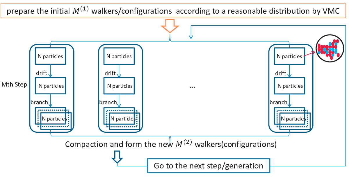
- Initialization
-
For the -particle system, first we need to choose the short-time step and M configurations (walkers) as the first generation, let us denote the M as . We then use M(RT)2 algorithm to make this configurations distributed according to the importance sampling wave function . In other words, we set the initial wave function as the importance sampling function . This step is carried out by the VMC procedure in which we also calculate the , and take this as the trial energy for the first generation.
- Drifting
-
Then, let us begin with the first walker in the initial configurations. In this walker, we drift all the particles in this walker one by one. The diffusion part of the Green’s function tells us that, for the particle, we can drift it from the old position to its possible new position according to
(B.49) where is a Gaussian random number with zero mean value and as variance, the subscript means the x, y or z component of the particle. The acceptance probability in the M(RT)2 algorithm should have . Now we use to judge if this move is accepted. In principle we should move all the particles (not one by one) in a walker at the same time, then judge if the new walker is accept. If the time step is small, the acceptance ratio of a good DMC run should be close to . In principle we should make sure the drift force is a constant during the time step (however this condition is actually violated, and that is why there is a linear term of time-step error in the extrapolation function). Anything violating the short-time approximation should be well-treated.
- Branching
-
Until here, the old walker with particles has been ‘drifted’ to the new walker . Now we need to do branching. Namely, we need judge how many of the new walkers do we need, zero (means we destroy the new walker), one, two, three or more? We judge this by first calculating
(B.50) and then
(B.51) here RAN means a uniform random number and INT means the integer part. Here the 2 is put by hand, we can use other values. This upper limit is to prevent more and more walkers sinking into abnormal regions where MB is very big which may cause incorrect distributions. If MB is 0, we destroy this walker. If MB is 1, we keep the walker. If , we keep MB copies of the new walker. Usually MB is around 1.
- Ergodicity
-
Until here, in the first generation of walkers, we have drifted and branched the first walker. Now we need to drift and branch all the rest of the walkers in the first generation. So we do it in this stage. Once we finished this, we go to compaction.
- Compaction
-
Now, all the walkers in the first generation has been drifted and branched. Some were killed, some remain, some were replicated. In this procedure we just remove those dead walkers and form the new number of walkers for the second generation.
- Population control
-
Once we obtain the walkers, we need to keep the number of walkers in each generations almost the same as the initial . The feedback mechanism I use is direct shrinking.
- Loop
-
Now we have the new generation of walkers, we then go to the loop, DriftingBranchingErgodicityCompactionPopulation controlDrifting, and the number of the loops is the number of the total generations. The number of generations is large enough such that all the excited states are removed, and the distribution of walkers are stabilized and is .
- Calculations
-
After enough generations of diffusion for the given time step , we sample from the stabilized generations. We take the average of those and find its error. We then do extrapolation to obtain the ground state energy with error bar.
APPENDIX C Auxiliary Field Diffusion Monte Carlo Brief
C.1 Formalism
DMC with or without importance sampling mentioned previously, can be taken as a special case of AFDMC (Schmidt and Fantoni 1999; Gandolfi 2007; Carlson et al. 2015). In general, in DMC simulations, the evolution of a state can be cast into such a form,
| (C.1) |
where X are a series of variables called auxiliary fields. Note that X are not necessarily coordinates. is the normalized probability density. is an operator acting on , it basically tells us how to move the walkers which form the state . As , we expect that the propagator is given by
| (C.2) |
We can think of as a linear combination of walker states with corresponding weight such that
| (C.3) |
where and denote the spatial and spinor (spin-isospin) part in a walker. Here the amplitude of different walkers are related by Kronecker delta .
The key is that, we sample from , then use to move each walker into the new walker with its weight ,
| (C.4) |
With importance sampling, we denote as a state such that we define
| (C.5) |
and that
| (C.6) |
In other words, it is
| (C.7) |
Consider that actually , the mixed average of operator can be written as
| (C.8) |
Putting Eq.(C.7) into Eq.(C.1) we have
| (C.9) |
Note that
| (C.10) |
Now we need a normalized distribution
| (C.11) |
in which the normalization factor
| (C.12) |
so that we can collect all the new walkers with less fluctuation. Neglecting , we have
| (C.13) |
where the local energy is given by
| (C.14) |
Now Eq.(C.9) can be written as
| (C.15) |
C.2 Hubbard-Stratonovich Transformation
The key of AFDMC is to reduce the quadratic dependence of operators to linear, with the Hubbard-Stratonovich transformation,
| (C.16) |
such that the interaction between nucleons can be conveniently cast into the form of DMC.
If possible, we can find ways to write a Hamiltonian into operators with quadratic dependence, that is
| (C.17) |
and then the DMC propagator(neglecting ) can be written as
| (C.18) |
neglecting , the normalized distribution can be written as
| (C.19) |
which means that is a gaussian random number with unit variance. In other words, we choose each auxiliary field by
| (C.20) |
We move each walker by such an operation
| (C.21) |
and the weight of the new walker is given by .
C.3 AFDMC and the Standard DMC with Importance Sampling
Let us consider the Hamiltonian
| (C.27) |
the approximated propagator after Hubbard-Stratonovich transformation is
| (C.28) |
For the importance sampling case,
| (C.29) |
and therefore the sampled auxiliary field are
| (C.30) |
the new walker with weight is moved by the translation operator,
| (C.31) |
which means that and
| (C.32) |
This is exactly the standard DMC with importance sampling introduced in Sec.B.3.
C.4 Quadratic Form of the AV6’ Interaction
The Hamiltonian with the AV6’ interaction for A-particle system can be written as
| (C.33) |
where the matrices are defined as
| (C.34) |
Here , , refer to , and components and , refer to the corresponding unit vector, and their eigenvectors and eigenvalues can be written as
| (C.35) |
We define the following operators,
| (C.36) |
such that the Hamiltonian can now be written in a quadratic form
| (C.37) |
which can be conveniently used in AFDMC.
C.5 Trial Wave Function
The trial wave function used in AFDMC for the -particle system has the following form,
| (C.38) |
where are the spatial coordinates and are the spin-isospin part of the system. For example can be written as
| (C.39) |
where , , and are complex coefficients for each basis.
The is composed of the Jastrow two-particle correlation functions and is given by
| (C.40) |
where is taken from the scalar component of the correlation operator in the Fermi-Hyper-Netted-Chain in the Single Operator Chain approximation (FHNC/SOC). The antisymmetric part of the trial wave function depends on the particular system to be studied. The general form is given by the non-interacting fermion wave functions in the Slater determinant,
| (C.41) |
where is a set of quantum numbers of single-particle wave function. It can be label as such that
| (C.42) |
where is a radial function, are spherical harmonics and are spinor part.
For uniform infinite nuclear matter, we can simulate the system by putting the particles in the periodic box of volume , and the single-particle function is given by the plane wave,
| (C.43) |
with integers , and the quantized momentum vector is given by
| (C.44) |
APPENDIX D AV6’ Linearizing Trick
Here I follow the note written by my advisor, and present how the six AV6’ operators in the propagator are linearized. First of all, notice that for non-negative integer , can still be express by the linear combination of the same 6 operators (just with different coefficients in front of the each operator). The 6 operators form a group. This is the foundation.
We then follow my advisor’s way of labeling the order of the operators. For a given pair, label them 1 and 2, we wish to calculate the AV6’ propagator linear in the 6 of its operators such that,
| (D.1) | |||||
where is the tensor operator in Eq.(2.20). We need to solve for the coefficients . We choose axis to be along in , and for the 6 operators we can find 6 states in terms of the total isospin quantum number and spin quantum number and its z component . We list the states and the corresponding eigenvalues for certain operators in Table D.1.
| Label | State | Degeneracy | |||
|---|---|---|---|---|---|
| 1 | 1 | 1 | 2 | 6 | |
| 2 | 1 | 1 | -4 | 3 | |
| 3 | -3 | 1 | 2 | 2 | |
| 4 | -3 | 1 | -4 | 1 | |
| 5 | 1 | -3 | 0 | 3 | |
| 6 | -3 | -3 | 0 | 1 |
Next, we sandwich between each of the 6 labeled states listed in Table D.1, and we get the 6 equations correspondingly,
From Eq.(D.1), we know that we need to solve for the coefficients from the already obtained values of ,
which can be written in the matrix form,
| (D.2) |
The coefficients can be solved by matrix inversion,
| (D.3) |
In other words, once we know , the coefficients are written as,
The six coefficients are the corresponding six in Eq.(2.74).
APPENDIX E Additional Calculations of the Response Functions
E.1 Angle Averaged Euclidean Response Functions
For any operator which is independent of the momentum , e.g., can be or defined in Eq.(4.48), we show how to take the angle average of momentum in calculating in the response functions.
In order to proceed, we first set up the coordinates as shown in Fig. E.1. The polar angle is , the azimuthal angle is , and . The length of is , its unit vector is , the , and components of are
| (E.1) | ||||
| (E.2) | ||||
| (E.3) |
The vector between particle and is defined as . Its length is , and its unit vector is and its components are , and .

Note that the plane wave can be expanded by spherical harmonics (Jackson 1999),
| (E.4) |
where are spherical Bessel functions (Abramowitz and Stegun 1964), and the spherical harmonics . In this calculation we only need those functions with .
For the spherical Bessel functions we need and ,
| (E.5) | ||||
| (E.6) |
For , the spherical harmonics of and are the same and they can be written as,
| (E.7) |
For , the spherical harmonics of can be written in terms of and as,
| (E.8) | ||||
| (E.9) | ||||
| (E.10) | ||||
| (E.11) | ||||
| (E.12) |
The spherical harmonics of for can be written in terms of , and as,
| (E.13) | ||||
| (E.14) | ||||
| (E.15) | ||||
| (E.16) | ||||
| (E.17) |
The Spherical harmonics are orthogonal such that
| (E.18) |
and they satisfy,
| (E.19) |
The following derived relations for spherical harmonics will be used,
| (E.20) | ||||
| (E.21) | ||||
| (E.22) | ||||
| (E.23) | ||||
| (E.24) | ||||
| (E.25) |
Before calculating the angle averaged response functions, we need to calculate several relevant angle averaged functions.
- 1.
Angle averaged function can be calculated as,
(E.26) - 2.
Angle averaged function can be calculated as,
(E.27) - 3.
Angle averaged function can be calculated as,
(E.28) - 4.
Angle averaged function can be calculated as,
(E.29) - 5.
Angle averaged function can be calculated as,
(E.30) - 6.
Angle averaged function can be calculated as,
(E.31) - 7.
Angle averaged function can be calculated as,
(E.32)
With the help of Eqs.(E.26) to (E.32), the 5 angle averaged response functions can be conveniently calculated.
- 1.
For the angle averaged nucleon coupling we have,
(E.33) - 2.
For the angle averaged proton coupling we have,
(E.34) - 3.
For the angle averaged isovector coupling we have,
(E.35) - 4.
For the angle averaged spin-longitudinal coupling we have,
(E.36) - 5.
For the angle averaged spin-transverse coupling we have,
(E.37)
E.2 Euclidean Response Functions in Different Coordinates
In all the , we can choose to be particle ’s absolute position, we can also choose to be particle ’s relative position in the center of mass frame. The response functions calculated using the center of mass multiply by a factor of will be those calculated using the absolute coordinate , where is the total mass of system. This can be explained by decomposing the separable Hamiltonian into the center of mass part , where is the total momentum, and a relative part first (Messiah 2014), then make use of the momentum translation operators.
The relevant part in Eq.(4.41) in absolute coordinate is
| (E.38) |
The total momentum of the ground state is 0, and the momentum translation operator will move particle ’s momentum by , therefore will change the system’s total momentum from 0 to and we have
| (E.39) |
Also consider that the Hamiltonian is translational invariant, so and therefore , so and commute, then Eq.(E.38) becomes,
| (E.40) |
The relevant part in Eq.(4.41) in the center of mass coordinate is
| (E.41) |
where is the center of the mass operator. Note that is also a momentum translation operator which changes the system’s total momentum by ,
| (E.42) |
So, the combined operator does not change the system’s total momentum. Therefore, the ground state’s total momentum remains zero after being operated by . Also, commutes with so and commute with each other. Taking all these into consideration, Eq.(E.41) becomes,
| (E.43) |
Comparing Eq.(E.40) and Eq.(E.43), we see that the center of mass result Eq.(E.43) need to multiply by the factor of to match the result in absolute coordinate Eq.(E.40). Take 4He as an example, in our plots, MeV/c, MeV/, , so the factor becomes . We calculate our response functions in the center of mass frame first because it will give lower variance compared with absolute coordinate (laboratory frame). We then multiply our results by in order to compare with the results in Carlson and Schiavilla 1994’s 1994 paper which are marked as the red dots in Figs. 4.12 and 4.13.
BIOGRAPHICAL SKETCH
Born in Shanghai, China on Feb 22, 1987, Rong Chen received his bachelor’s degree from Shanghai University in June, 2009. With postgraduate recommendation, he was directly admitted by Shanghai Jiao Tong University as a master degree student in August 2009, where he worked with prof. Lie-Wen Chen on various topics of infinite nuclear matter with isospin-dependent phenomenological nucleon-nucleon effective interactions. He received the Master of Science degree in June 2012 from Shanghai Jiao Tong University. In August 2012, he entered Arizona State University to pursue his PhD degree, and he worked as teaching and research assistant thereafter. He did research rotations with profs. Cecilia Lunardini during fall 2012 about neutrino physics and Tanmay Vachaspati during spring 2013 about cosmology. Then he worked with prof. Lunardini again from fall 2013. However the cooperation reached an end in early 2014, due to some reason which may only be fully understood after many years. Therefore his PhD career was once entwined with neutrinos, but never joined. At that time the chair of the graduate program committee prof. Ralph V. Chamberlin introduced him to prof. Kevin E. Schmidt, who kindly accept him as one of his graduate students without too much hesitations. He started to worked with prof. Schmidt since mid 2014 on quantum Monte Carlo calculations. The first project from mid 2014 to late 2016 about the inclusion of the full three-body interactions in the approximated propagator in auxiliary field diffusion Monte Carlo was not successful enough to lead to a PhD project. During summer 2016, he attended the TALENT School on Nuclear Quantum Monte Carlo Methods held in North Carolina State University, which was mainly organized by prof. Dean Lee. Late 2016 was the turning point, with prof. Schmidt’s suggestion and patient guidance, he began to work on the first continuous space path integral quantum Monte Carlo calculations of light nuclei, which became his Ph.D project and publishable results were obtained. He gave a talk about it at 2019 Annual Meeting of the APS Four Corners Section. He successfully defended his PhD dissertation on July 9, 2020.