Analyzing Planar Galactic Halo Distributions with Fuzzy/Cold Dark Matter Models
Sangnam Park, Dongsu Bak, Jae-Weon Lee, Inkyu Park
a) Natural Science Research Institute, University of Seoul, Seoul 02504, Korea
b) Physics Department, University of Seoul, Seoul 02504, Korea
c) Department of Electrical and Electronic Engineering, Jungwon University
85 Munmuro, Goesan, Chungbuk 28024, Korea
(u98parksn@gmail.com, dsbak@uos.ac.kr, scikid@jwu.ac.kr, icpark@uos.ac.kr)
ABSTRACT
We perform a numerical comparison between the fuzzy dark matter model and the cold dark matter model, focusing on formation of satellite galaxy planes around massive galaxies. Such galactic dynamics with controlled initial subhalo configurations are investigated using GADGET2 for the cold dark matter and PyUltraLight for the fuzzy dark matter, respectively. We demonstrate that satellite galaxies in the fuzzy dark matter side have a tendency to form more flattened and corotating satellite systems than in the cold dark matter side mainly due to the dissipation by the gravitational cooling effect of the fuzzy dark matter. Our simulations with the fuzzy dark matter typically show the minor-to-major axis ratio of the satellite galaxy planes to be ; This well matches the current observed value for the Milky Way.
1 Introduction
Numerical simulations based on the cold dark matter (CDM) model successfully reproduce the observed large-scale structures of the universe. However, it encounters difficulties in explaining small-scale structures around galactic scales. For example, the CDM model predicts a cusped central halo density which is not observed and too many dwarf galaxies around massive host galaxies than the observed [1, 2, 3, 4].
On the other hand, the satellite-plane problem is another serious small-scale challenge for the CDM model (see [5, 6] for a review). Observations indicate that a substantial fraction of satellite galaxies around the Milky Way, Andromeda and Centaurus A co-orbit in flattened planar structures [7, 8]. At least 10 highly flattened planes of dwarf galaxies have been discovered [9]. This is in sharp contrast with cosmological simulations with the CDM, which show much more random distributions and motions of satellite galaxies. The probability of finding such flattened co-rotating satellite systems with the CDM is very low [5, 7] although the statistic is controversial.
It is not easy to explain these satellite planes theoretically in the CDM model. Disks in astronomical objects such as a protoplanetary disk or a black hole accretion disk form when falling matter such as gas loses its energy by a dissipation (cooling) mechanism while keeping the angular momentum of the matter. For a given angular momentum, the lowest energy state is a disk orthogonal to the rotation axis [10]. Similarly, to form a flat disk-like structure small galactic halos should lose their gravitational energy by some dissipation mechanism when they fall towards heavy central galaxies. However, the typical collisionless CDM model lacks an efficient mechanism for this to happen. Due to the large scales baryonic processes could not strongly affect the satellite planes.
As an alternative to the CDM, there is a growing interest in the fuzzy dark matter (FDM) [11, 12, 13, 14, 15], also known as ultra-light axion or scalar field dark matter. In this model, dark matter (DM) particles satisfying the Schrödinger-Poisson equation have an ultra-light mass and a long de Broglie wavelength , where is the velocity of the dark matter particles. (See [16, 17] for more references.) Unlike CDM particles, condensed FDM particles behave as a coherent wave, and due to the quantum uncertainty principle the FDM has a typical length scale which suppresses the formation of DM structures smaller than a galaxy core and helps resolve the aforementioned small-scale issues [16].
While the CDM model has no efficient dissipation mechanism to make the observed satellite systems, a gravitational cooling effect in the FDM model provides a unique and efficient dissipation mechanism for them. The gravitational cooling [18, 19, 20] is a mechanism for relaxation by ejecting part of the FDM density and carrying out excessive kinetic energy and momentum. In this mechanism colliding FDM halos can have interfering wave profiles which contain high momentum modes. These modes can easily escape the gravitational potential of the halos carrying out energy.
The main aim of this paper is to show that halos in the FDM model have a tendency to form a more flattened and corotating satellite plane than in the standard collision-less CDM model11 1 Mixed state solutions of the Schrödinger-Poisson equation were suggested to be a cause of the anisotropic concentration of satellite galaxies [21], which is different from our proposal.. To show this tendency we perform numerical simulations of formation of toy galactic systems using Gadget2 for the CDM and PyUltraLight for the FDM, respectively. Since it is challenging to simulate a full-fledged cosmological structure formation with the FDM due to the wave nature of the model, we restrict ourselves to studying the differences in structure formation at galactic scales with controlled initial conditions for seed satellite galaxies in the two models. (There are cosmological scale hydrodynamical simulations with FDM and baryon matter for structure formation [22].)
In Section 2 we describe our numerical simulation setup for formation of galactic systems in the FDM and the CDM models. We shall apply the numerical results to find the motion of satellite galaxies using the so called Mulguisin halo finder. Section 3 contains the results of our numerical study. We analyze and compare resulting satellite distributions of the two DM models. In Section 4 we compare our results with the observed astronomical data. The last section is devoted to concluding remarks.
2 Simulation Setup
In this section, we would like to describe our simulation setup for the above two DM models. As was mentioned already, we are not trying to do a full-fledged cosmological simulation, which is certainly beyond scope of our current study. Rather, we setup specific initial configurations for the late-time formation of galactic satellite systems, focusing on the purely gravitational dynamics in a fixed flat background. Our primary aim is to see the resulting differences between the FDM and the CDM dynamics.
2.1 FDM subhalo seeds
Our FDM dynamics are governed by the Schrödinger-Poisson equations
| (2.1) | ||||
| (2.2) |
where is the mass of ultralight scalar particles, for the Newton constant, and denotes the total mass of the galactic system of interest. The wave function is a complex function of spacetime normalized as , the corresponding FDM mass density then given by , and for the gravitational potential produced by the density . The value is the fiducial mass suggested to solve the small scale problems such as the missing satellite problem. If we use a much larger value for we expect the wave nature of FDM becomes less relevant and the difference of FDM from CDM becomes less prominent.
As an initial subhalo configuration, we shall use the ground state solution (see e.g. [16]) of the Schrödinger-Poisson system with a mass , which will be called a ‘soliton’ below for simplicity [23]. Let us denote this soliton wave function centered at by , whose explicit functional form is known numerically22 2 We take this to be real without introducing any extra phase at this stage. In [24], an approximate fit function of this soliton configuration was introduced as where is the half mass radius. This form will not be used in our simulation below.. It is also known that the half mass radius of the soliton is given by [16]. This soliton configuration is spherically symmetric, stable under a small perturbation, and may work as a seed for late-time satellite galaxies in our simulation. Although we are not explicitly presenting it in this note, a moving soliton solution with a constant velocity is rather well known in terms of the above wave function [25]. Using this, one may obtain an initial wave function [25]
| (2.3) |
describing an initial condition for a soliton with an initial velocity centered at an initial position . The phase will be assigned randomly for each soliton below. In this note, we shall take the initial subhalo mass to be leading to kpc. This choice, which is slightly larger than the typical satellite mass of nearby galaxies, was made because, through interactions with the rest, the seeds generically lose their mass in the formation of their satellite system.
For our FDM simulation, we shall use the python pseudo-spectral solver, PyUltraLight, developed in [25], which is publicly available. In this package, the whole system is placed in a box of size with a periodic boundary condition . We shall take the box size to be kpc and the number of the grid points () in each direction is set to . Hence our spatial resolution becomes kpc. We choose the simulation time-step, Myr, which is slightly smaller than the default value of the python code, Myr. See [20] for a detailed explanation of a similar choice. In PyUltraLight, the full initial wave function is prepared by a simple superposition of the initial soliton wave functions describing initial subhalo seeds with given velocities. To avoid any significant overlap contributions, we separate initial positions such that one may ignore their overlap contributions. With this initial configuration, the Schrödinger-Poisson equations are solved with the above specified boundary condition, which produces time-series sets of wave-function maps leading to an evaluation of relevant physical quantities such as density maps.
2.2 CDM subhalo seeds
We now turn to our simulation setup in the CDM side. Here we shall basically perform a gravitational -body simulation using Gadget2 [26] which is also publicly available and we would like to imitate our initial FDM halo configurations as much as possible. Specifically, we set the mass of the initial subhalo to be as before and use the same sets of initial positions and velocities as the FDM counterparts. However, a stable solitonic configuration is not available in the CDM side. We instead prepare an initial CDM subhalo based on the NFW profile [2] whose mass density function is given by
| (2.4) |
where is the length scale of the profile. In particular we generate () CDM particles with a mass , whose initial positions are randomly allocated following the NFW profile with a cut-off scale set by . The two parameters, and are fixed by the conditions
| (2.5) | ||||
| (2.6) |
where will be further adjusted in the following way. We set these particles to move only in angular directions, selected randomly, and their speed to with a judicious choice of where denotes the total mass of particles within a radius . Now performing a separate -body simulation, we let the subhalo system evolve for Gyr such that the subhalo particle system is relaxed into a dynamical equilibrium. We adjust the initial parameter such that the resulting half mass radius agrees with that of the FDM soliton (). In fact we found that with the above choice of . We then use the resulting particle positions and velocities as our actual initial subhalo configuration. This relaxed configuration slightly differs from the original NFW profile we began with. However we view that this does not matter due to the following two reasons; First the NFW profile would not be that precise configuration that follows from the CDM simulations [27, 28]. Second we tried other models such as the Plummer and the above soliton and found that the resulting differences are rather negligible.
Gadget2 is a cosmological -body simulation code based on the so-called TreeSPH code, by which one may compute the nonlinear regime of gravitational dynamics and hydrodynamics. In the simulation, with particles, we first assign their initial positions and velocities, and evaluate their gravitational time evolution by computing the gravitational force on each particle using a TreePM algorithm (see [26] for the details).
In our CDM simulation, we again put the -body system inside a box with a size together with the spatially periodic boundary condition. In the simulation with Gadget2, we also set the particle mesh grid (PMG) scale to kpc. This choice may offer a computational efficiency without much loss of the accuracy in the calculation of forces based on the purely Tree algorithm. We set the softening length (SL) scale to value . This requirement (SL ) is needed to prevent any strong discreteness effects where plays a role of setting the upper limit of acceleration in two-body encounters by the mean-field value of a subhalo [29]. We have also tested more smaller scale SL′ , which ensures preventing large-angle deflections in two-body encounters [29]. We have tried various such choices and found that there are no significant differences in their performances.
We make our resulting datasets of CDM density fields with the same resolution as those of the FDM side for an unbiased comparison of the two sides. In this analysis, we use the Pynbody package [30] which is an open source code especially suitable for astrophysical -body and smoothed-particle hydrodynamics (SPH) problems. We down-size the datasets of three dimensional density fields from original 900 cells along each side of the simulation box to 450 cells, which is mainly for our computational convenience while keeping the accuracy needed for an identification of the satellite galaxies. These satellites, in the present case, as small clusters of DM distribution will be identified with Mulguisin halo finder, whose details are described below.
2.3 Initial halo configuration
In order to prepare our initial configuration for seed subhalos, we use the Plummer model [31] whose density profile is described by
| (2.7) |
where denotes the half light radius. This model is chosen to simply provide enough randomness for our initial halo configuration. We shall set kpc, which seems an appropriate choice compared to the size of our simulation box. Including the velocity dependence, the distribution function becomes
| (2.8) |
if and otherwise, where . Our initial halo configuration will be consisting of seed subhalos. In each set of this initial configuration, we begin by randomly generating subhalo positions and velocities following the above distribution function. In order to prepare an out-of-equilibrium configuration, we shall then multiply an overall factor to the above generated velocity for each seed subhalo. For the smaller (and also for introduced right below), the initial halo configuration becomes the more tightly bound gravitationally and, of course, the more subhalos are then infalling to the central region.
Now in order to provide an overall angular momentum for our initial halo configuration, we proceed as follows. With the above prepared initial set for total 200 subhalos, we randomly select subhalos and add an angular velocity to each of them where is the rotation velocity with denoting the sum of masses within the radius from the center of the box. To the remaining subhalos, we add . Thus the resulting initial velocity becomes
| (2.9) |
for the or the remaining subhalos, respectively. Finally we translate, rotate and boost the above halo system such that it has a vanishing center of mass position and velocity involving only a component of total angular momentum. The parameters and are introduced to obtain an appropriate spin of our halo. Of course, the random choice of the subhalos may provide an extra randomness for our initial subhalo configuration. In order to consider a well-bound system, one has to restrict the parameter regime to where is roughly characterizing the kinetic energy contribution of the initial halo system.
In measuring the spin of our halo system, we shall adopt the dimensionless spin parameter [32]
| (2.10) |
where denotes the magnitude of total angular momentum and the total energy of the system. From the CDM-based Millennium simulation [33], the average value of the spin parameter for its field halos is estimated as [34].
In this note, we shall consider five cases of . The parameter will be fixed to be . Then, for each choice of and , we shall adjust to match the initial spin parameter of our initial halo configuration with the above value approximately within % errors. In this manner, one finds for respectively. Finally we repeat our simulation times for each choice of where initial subhalo positions and part of velocities () are fully randomly generated for each simulation. Below we shall refer the resulting initial condition specified by to “initial condition ” since, with specified, and are fully fixed in the above choices of initial conditions. In our CDM simulations below, these choices of initial parameters will lead to a typical CDM flattening of satellite distributions derived from full cosmological simulations under CDM (see Section 4 for the details). One may try larger values of such as or even larger. The resulting initial configurations are no longer gravitationally bound; With , one indeed finds that part of subhalos go out of the simulation box and also that the late-time relaxation of the system is hardly achieved due to the relatively large kinetic energy. Therefore such choices will be inappropriate as our proper initial setup.
We set our total simulation time to be Myr, which corresponds to a total of 2400 time steps (in ). However, we find that some of the subhalos after initial collisions may go out of the box through one side and reappear through its opposite side, which is basically due to the periodic boundary condition imposed in this note. To avoid such instances with enough margin, we shall take the validity limit of our simulation time to be Myr.
2.4 Halo reconstruction
Given the initial halo configuration, the simulations using PyUltraLight for FDM and Gadget2 for CDM are performed. For each time step, we save both FDM and CDM density maps for further halo reconstruction and data analysis. Galaxies and halos are the gravitationally bound objects and they appear as clusters in the density map data. A cluster can be defined as a large collection of points or cells in a small area or a localized volume. Cluster finding has been a popular topic in computational science. Many different clustering algorithms are available which have been developed and maintained by many different groups. As each clustering algorithm has its own strength and weakness, one should carefully choose the right algorithm for their own research purpose.
In this study, we have adopted the Mulguisin clustering algorithm, which has been used in particle physics for finding jet structures from the collection of particle tracks [35]. The algorithm was modified to find clusters out of input cells in 3D space. It first finds the most massive cell in the input data and name it a seed. Then it looks for the next massive cell which will be used as a test cell. If the test cell is close enough to the seed, we then attach the cell to the seed and these two cells become a group. A group can therefore be regarded as a list of cells. If the distance between the test cell and the seed is longer than a certain cut length, then it becomes a new seed. In this study we use 1.4 kpc as out distance cut length.
Now the same procedure is repeated for the next massive cell. The cell will be attached to a group when the minimum distance between the test cell and the group is shorter than the cut length. For this we calculate all distances between the test cell and the cells in the group and choose the minimum value. Once again, if the test cell does not join to any existing groups then it becomes a new seed. The algorithm keeps doing this simple process until there are no test cells left. At this stage, cells are all converted to groups. Some groups are big, i.e. have many cells, and some are not. There are also single-cell groups that are isolated from other groups.
At this stage a group is called a when its mass is larger than a certain mass cut. Clusters are then further tested to see whether they form a super-cluster. A super-cluster can therefore be regarded as a pack of clusters that are attached with each other. The minimum distance between two clusters is calculated from the whole combinations of cells from each cluster and it is used to decide whether the two clusters are to be merged or not. We use the same distance cut of kpc for the merging process.
All these procedures are implemented in our Mulguisin halo finder software. Figure 2 shows the results from cluster finding by the Mulguisin algorithm. The clusters that were found by the halo finder are marked with black circles.
3 Numerical Results
In this section we shall present the outcome of our numerical study. In Figure 1 we depict the time evolution of DM density during the formation of sample galactic halos (either in the CDM or the FDM model) as a time series of projected DM density maps in the unit of . To make these projected maps, the mass density fields of each halo system are integrated over the range along -direction (the left two columns) or -direction (the right two columns) of the simulation box. Also for these maps, we used the samples from the simulations for the initial condition. Note that both the CDM and the FDM halo density maps shown in the figure are from simulations with the same initial positions and velocities of subhalos.

The CDM and the FDM halo system look quite similar at the early stages of the evolution process. But after the collapse of initial subhalo systems as illustrated in the second row of Figure 1, their difference becomes clear as will be further described below: In the CDM side, there appear far more surviving subhalos, especially around the central region, than the FDM counterpart, and so is more substructure on the smallest scales. On the length scales of the whole parent halo, however, the tentacle-like structure found at late times is more prominent in the FDM than the CDM side.
Among clusters found by the Mulguisin algorithm, we shall identify objects with mass greater than 33 3 This mass-cut is introduced to eliminate too small clusters such as globular clusters. as satellites, which were all marked with small black circles on the projected maps in Figure 2. We find that the CDM system has roughly eight times more satellites than the FDM side. While there are many satellites in the central region of the CDM halos, the FDM halos involve almost none in that region. One may also see that the FDM satellite distributions appear more flattened than the CDM counterparts, even before analyzing any details. One can also see the outgoing waves from the gravitational cooling in the FDM side.

To be more concrete, we shall focus on the following three choices of initial conditions, , particularly for Figures 3–6 and their discussions.
First let us introduce the ratio of the semi-minor to the semi-major axis (denoted as ) of an ellipsoid derived from a satellite distribution [36, 37, 38] in the following manner. Its principal axes are defined using the mass tensor of satellites
| (3.1) |
where refers to the position of the -th satellite and denotes the total number of satellites in each halo system. Note here that the origin of the position is defined by the center of mass in each halo system where its density peak is also located approximately. In fact, with our choice of initial halo configuration, this center of mass was set to agree with the center of the simulation box, and shall be simply called the center below. The eigenvalues of the tensor (ordered by ) define the corresponding principal semi-axes respectively by , , and .

In Figure 3, we depict the time evolution of , i.e. the average of for the 30 simulation samples prescribed in Section 2.3, from the initial time to Myr. In each plot, the black dash-dotted line is for the of satellites system in the CDM halo model, the red solid for that of the FDM, the green dashed for their difference, and the blue dotted for the ratio of the latter over the former. The error bars in each plot represent the estimation for the standard deviation of the 30 simulation samples. It is clear that the FDM satellite profiles lead to a smaller than their CDM counterparts. In addition, for both the FDM and the CDM, one finds that gets larger as becomes larger. This is because, as becomes larger, the average strength of each random velocity in our initial halo configuration increases.

The rms height is the rms of vertical distances of satellites from their best-fit-plane [38] that is determined by minimizing
| (3.2) |
with respect to where is a unit normal vector to the would-be best-fit-plane. In other words the best-fit-plane is obtained with all satellites in the whole simulation box. In fact, the corresponding unit normal vector determined in this manner almost agrees with the eigenvector given above. One further introduces the rms height calculated only with the satellites within the horizontal distance from the center, in which the best-fit-plane and unit normal vector are in advance fixed by the minimization procedure of in (3.2). In Figure 4, we depict the rms height of satellites as a function of the horizontal distance from the center at Myr, where we have taken kpc because we would like to avoid the centroid residing in the region within kpc. We may confirm that the FDM systems have thinner satellite planes than the CDM counterparts. In particular, one finds that, for kpc, the FDM rms height grows while the CDM counterpart does not change appreciably for the same range. This happens because, in the CDM side, for the above range of already many satellites are found with a significantly build-up value of the rms height. On the other hand, in the FDM side, there are not many satellites in that region and their rms height is building up from relatively small values.
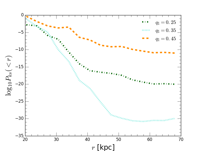
An alternative to the ratio is the -dependent cumulative distribution function (CDF) 44 4 Slightly abusing notation, we shall denote the full CDF including the whole satellites simply by . of a satellite system where one includes only satellites within the radius from the center and is given by with being the position of a satellite and denoting the unit eigenvector corresponding to the eigenvalue . We shall use the Kolmogorov-Smirnov probability by comparing CDF samples of the FDM/CDM satellite systems where each CDF denoted by is drawn from the angular positions of satellites in all 30 samples for each choice of initial condition55 5 In general this quantity represents the probability that any two sets of samples were drawn from the same cumulative probability distribution, where the probability is determined by the so-called Kolmogorov CDF whose argument is given by with denoting the size of the -th sample and the Kolmogorov-Smirnov statistic characterizing the maximal difference of two CDF’s.. With the CDF’s as well as , we may deduce the main underlying factors that make the FDM halo system have a more flattened satellite system than its CDM counterpart.

In Figure 5 we illustrate the CDF for the three initial conditions of our main interest. For each initial condition, this CDF with a subscript is made by merging all the data points in each set of the 30 samples as explained in Section 2.3. The black dash-dotted line is for the CDM, the red solid for the FDM, and the blue dashed corresponds to the reference spherically symmetric distribution. These plots clearly show that, for both the FDM and CDM models, the CDF’s are quite distinguished from the spherically symmetric distribution. They also imply that the FDM model leads to more anisotropic satellite systems than their CDM counterpart. Figure 6 shows the -dependent Kolmogorov-Smirnov probability where one includes those satellites within the radius from the center in order to build . From Figure 4, one may easily guess that the Kolmogorov-Smirnov statistic may decrease as a function of especially for the region of near the centroid. However, the number of satellites increases as grows. Indeed the latter growth effect becomes dominant, which leads to the monotonically decreasing behaviors of as a function of as illustrated in Figure 6.
In Table 1, our measures for the flattening of satellite planes are summarized including the Kolmogorov-Smirnov probabilities between the CDM and the FDM distribution. All data are drawn from the samples at Myr. All of our initial conditions with are included in this table. These results show that the FDM and the CDM satellite system behave differently from each other.
| IC | c/a (meanstd) | (meanstd) [kpc] | |||
|---|---|---|---|---|---|
| CDM | FDM | CDM | FDM | ||
| 0.25 | 0.4060.044 | 0.2230.073 | 9.3010.770 | 6.8721.987 | 1.243 |
| 0.30 | 0.4150.049 | 0.2220.063 | 9.2300.791 | 6.7371.789 | 1.135 |
| 0.35 | 0.4660.053 | 0.2360.067 | 9.9610.811 | 6.8321.875 | 1.047 |
| 0.40 | 0.4950.068 | 0.2670.108 | 10.4051.226 | 7.5482.676 | 2.069 |
| 0.45 | 0.5320.071 | 0.2950.120 | 10.6891.237 | 8.0682.735 | 4.574 |
As mentioned in Introduction, all the satellites systems in our FDM halo models result in more flattened planes than those in the CDM counterparts with respect to all measures in this work. This trend may also be seen from the Kolmogorov-Smirnov probability given in the Table 1 for various initial conditions. Roughly speaking, the more similar the two distributions come to be, the larger is the corresponding Kolmogorov-Smirnov probability . As becomes smaller, the initial collapse gets stronger, more subhalos are colliding into the central region, and the resulting satellite system becomes more flattened. Notice that these collisions mostly occur at an early stage of the evolution processes. The relatively stronger flattening in the FDM side is closely tied to the gravitational cooling effect, which is especially effective around the central region of the halos. It should be commented that should be correlated with the parameter but, in Table 1, it does not increase monotonically nor does it show any clear trend with . This is simply because concerns about the difference between the two CDF’s and the flattening trends of FDM and CDM may differ from each other.
We now turn to the corotation ratio where denotes the number of satellites involving a positive/negative -component respectively. With the initial condition, one begins with both for the FDM and the CDM halo. At Myr, we find the FDM corotation ratio , which is bigger than the CDM value . The resulting FDM ratio appears to be more consistent with observational data, but this requires further studies.
Finally let us comment upon satellite orbital poles, and in particular their standard deviation [39] defined by
| (3.3) |
where is the normalized mean vector of orbital poles given by with . Note that this definition is somewhat different from the usual one in literature where the value from 7 or 8 best aligned angular momenta of the most massive satellites is taken.
We find a narrower distribution of FDM satellite orbital poles with than the CDM side with ; these numbers are drawn from the samples with the initial condition at Myr.
4 Comparison with observational data
For a thorough understanding of the galaxy formation problem, one has to perform a full-fledged cosmological simulation from the very early universe as was mentioned before. Since our results in this note are based on the simplified toy galaxy models of typical size kpc while adopting specific initial conditions, it is hard to compare our numerical results directly to observational data from real galaxies. Nonetheless, it is interesting to see that our toy galaxy models in the FDM side much resemble the observed at least qualitatively as discussed right below.
According to observations, the satellite planes of the Milky Way typically possess an rms height kpc, axis ratio , standard deviation of orbital poles 66 6 As previously mentioned, the definition of in the references is different from ours. and inclination angle [5, 40] depending on the sample. Similarly, the Centaurus A satellite system has kpc, and [41].
Our simulations in the FDM side typically show and (with the initial condition), which well agree with the above observed values for the Milky Way. Our simulations in the CDM side, on the contrary, exhibit typically and (with the initial condition), which are larger than the observed ones. These values for the CDM are consistent with those of the planes of satellite galaxies in the EAGLE simulation with the CDM [36]. Thus one may say that the FDM model works better at reproducing the observed satellite plane structures than the CDM counterpart.
On the other hand, the rms heights for the both DM models are around kpc, which appears smaller than the observed. This discrepancy may be attributed to the relatively smaller size of the simulated centroid (carrying a typical mass ) than that of the observed central galaxies possessing a heavier typical mass . Assuming a similar average DM density for all galaxies, the spatial size of the heavier galaxies may become [ ] times larger than the simulated value. Therefore, we expect kpc for the heavier galaxies, which is indeed comparable to the observed. To confirm this we need a simulation with a larger box, which is beyond the scope of this paper.
We interpret our numerical results in the following way. Energy loss with a conserved angular momentum during a collapse usually leads to a formation of a highly flattened astronomical structure. In both dark matter models, during the collapse satellites gravitationally exchange their energy and momentum with others and experience a kind of an averaging process. Those satellites getting a relatively large angular momentum during the process may escape the central region and easily survive, while satellites with a small angular momentum tend to fall into the central region.
In the FDM side satellites which get small angular momentum and fall into the central region can be absorbed into the centroid by losing their energy via the gravitational cooling effect. Apparently, in our simulations a large portion of the falling satellites in the FDM side are tidally disrupted and lose their cores and disperse completely. As a result surviving satellites in the FDM side have a tendency to form corotating planar structures orthogonal to the total angular momentum vector. Note that this effect is clearly seen in Figure 1.
On the other hand, a large portion of similar falling satellites in the CDM side may survive the crossing through the centroid in the same situation, mainly due to the particle nature of the CDM model. Thus, we expect satellites in the CDM model without an efficient energy loss mechanism redistribute themselves more spherically than in the FDM model as seen in Figure 2.
In our scenario we also expect that the width of a satellite plane in the FDM side could be roughly related to the size of the centroid, because the spatial size of the centroid provides a typical length scale for the satellite absorption process near the centroid which is responsible for the energy loss and the formation of the satellite planes as previously mentioned.
Another interesting observation is that, even with the same initial conditions, there are less FDM satellites surviving compared to the CDM side due to the same effects making satellite planes. This hints yet another route in the FDM model to solve the missing satellite problem of the CDM model, because the typical solution in the FDM model to the problem is usually attributed to the suppression of the initial matter spectrum [11] compared to the CDM model.
For more conclusive results we need more realistic simulations for larger galaxies, which is beyond the scope of this work. Since our simulations are DM-only simulations, they do not provide information of inclination angles of the satellite planes with respect to the galactic disks.
5 Conclusions
In this note, we have numerically shown that galactic satellite systems in the FDM model are more flattened and corotating than their CDM counterpart. This is basically due the gravitational cooling effect in the FDM side especially near the central part of galaxies. This energy loss mechanism is a unique feature of the FDM which is absent in other alternatives of the CDM such as warm dark matter. Our toy galaxies in the FDM model seem to reproduce the observational features such as axis ratios of the satellite planes.
Our work implies that the FDM model could be a way to solve the problem of the satellite-galaxy planes as well as other small scale tensions. Thus the galactic satellite planes could serve as a good test bed for dark matter model discrimination. For more conclusive results, cosmological simulations with baryons starting from more realistic initial conditions are certainly required, which we leave for our future studies.
Acknowledgement
We would like to thank the referee for very constructive suggestions and Andreas Gustavsson for careful reading of the manuscript. Sangnam Park was supported in part by Basic Science Research Program through National Research Foundation funded by the Ministry of Education (2018R1A6A1A06024977). Dongsu Bak was supported in part by NRF Grant 2020R1A2B5B01001473, and by Basic Science Research Program through National Research Foundation funded by the Ministry of Education (2018R1A6A1A06024977). Jae-Weon Lee was supported by NRF-2020R1F1A1061160. Inkyu Park was supported by the 2021 Research Fund of the University of Seoul. This work was also supported by the UBAI computing resources at the University of Seoul.
References
- [1] P. Salucci, F. Walter and A. Borriello, Astron. Astrophys. 409, 53-56 (2003).
- [2] J. F. Navarro, C. S. Frenk and S. D. M. White, Astrophys. J. 462, 563-575 (1996).
- [3] W. J. G. de Blok, A. Bosma, and S. S. McGaugh, astro-ph/0212102 (2002).
- [4] A. Tasitsiomi, International Journal of Modern Physics D 12, 1157 (2003).
- [5] M. S. Pawlowski, Mod. Phys. Lett. A 33, no.06, 1830004 (2018).
- [6] M. S. Pawlowski, Galaxies 9, no.3, 66 (2021).
- [7] O. Müller, M. S. Pawlowski, F. Lelli, et al., 645, L5. Astron. Astrop. (2021).
- [8] I. M. Santos-Santos,R. Dominguez-Tenreiro, M. S. Pawlowski, Mon. Not. Roy. Astron. Soc., 499, 3755. (2020).
- [9] Libeskind N. I., et al., 2019, MNRAS, 490, 3786 (2019).
- [10] J. E. Pringle Annual Review of Astronomy and Astrophysics, 19:1, 137 (1981).
- [11] W. Hu, R. Barkana, and A. Gruzinov, Phys. Rev. Lett. 85, 1158 (2000).
- [12] M.R. Baldeschi, G.B. Gelmini, R. Ruffini, Physics Letters B 122, 221 (1983).
- [13] M. Membrado, A.F. Pacheco, J. Sañudo, Phys. Rev. A 39, 4207 (1989).
- [14] S.J. Sin, Phys. Rev. D50, 3650 (1994).
- [15] J.W. Lee, I.G. Koh, Phys. Rev. D53, 2236 (1996).
- [16] L. Hui, J. P. Ostriker, S. Tremaine and E. Witten, Phys. Rev. D 95, no. 4, 043541 (2017).
- [17] J. W. Lee, EPJ Web Conf. 168, 06005 (2018). [arXiv:1704.05057].
- [18] F. S. Guzman and L. A. Urena-Lopez, Astrophys. J. 645, 814 (2006).
- [19] D. Bak, S. Kim, H. Min and J. P. Song, J. Korean Phys. Soc. 74, no. 8, 756 (2019).
- [20] D. Bak, J. W. Lee and S. Park, J. Korean Phys. Soc. 79, no.6, 582-588 (2021).
- [21] J. Solis-Lopez, F. S. Guzman, T. Matos, V. H. Robles and L. A. Urena-Lopez,’ Phys. Rev. D 103, no.8, 083535 (2021).
- [22] P. Mocz, A. Fialkov, M. Vogelsberger, F. Becerra, M. A. Amin, S. Bose, M. Boylan-Kolchin, P. H. Chavanis, L. Hernquist and L. Lancaster, et al. Phys. Rev. Lett. 123, no.14, 141301 (2019).
- [23] P. Chavanis, Phys. Rev. D 100, no.8, 083022 (2019).
- [24] H. Y. Schive, M. H. Liao, T. P. Woo, S. K. Wong, T. Chiueh, T. Broadhurst and W. Y. P. Hwang, Phys. Rev. Lett. 113, no.26, 261302 (2014).
- [25] F. Edwards, E. Kendall, S. Hotchkiss and R. Easther, JCAP 10, 027 (2018).
- [26] V. Springel, Mon. Not. Roy. Astron. Soc. 364, 1105-1134 (2005).
- [27] J. S. B. Wyithe, E. L. Turner and D. N. Spergel, Astrophys. J. 555, 504 (2001).
- [28] A. A. Dutton and A. V. Macciò, Mon. Not. Roy. Astron. Soc. 441, no.4, 3359-3374 (2014).
- [29] C. Power, et al., Mon. Not. Roy. Astron. Soc. 338, 14-34 (2003).
- [30] A. Pontzen et al., Astrophysics Source Code Library, ascl:1305.002 (2013).
- [31] H. C. Plummer, Mon. Not. Roy. Astron. Soc. 71, 460-470 (1911).
- [32] P. J. E. Peebles, Astrophys. J. 155, 393 (1969).
- [33] V. Springel, S. D. M. White, A. Jenkins, C. S. Frenk, N. Yoshida, L. Gao, J. Navarro, R. Thacker, D. Croton and J. Helly, et al. Nature 435, 629-636 (2005).
- [34] P. Bett, V. Eke, C. S. Frenk, A. Jenkins, J. Helly and J. Navarro, Mon. Not. Roy. Astron. Soc. 376, 215-232 (2007).
- [35] M. Bosman et al., ATLAS-SOFT-98-038 (1998).
- [36] S. Shao, M. Cautun and C. S. Frenk, Mon. Not. Roy. Astron. Soc. 488, no.1, 1166-1179 (2019).
- [37] S. Shao, et al., Mon. Not. Roy. Astron. Soc. 460, no.4, 3772-3783 (2016).
- [38] A. R. Zentner, A. V. Kravtsov, O. Y. Gnedin and A. A. Klypin, Astrophys. J. 629, 219 (2005).
- [39] M. S. Pawlowski, et al., Mon. Not. Roy. Astron. Soc. 442, no.3, 2362-2380 (2014).
- [40] M. S. Pawlowski, & P., Kroupa, Mon. Not. Roy. Astron. Soc. 491,3042 (2020).
- [41] R. B. Tully, et al., Astrophys. J. Lett. 802, L25 (2015).