Current Trends in Deep Learning for Earth Observation:
An Open-source Benchmark Arena for Image Classification
Abstract
We present AiTLAS: Benchmark Arena – an open-source benchmark suite for evaluating state-of-the-art deep learning approaches for image classification in Earth Observation (EO). To this end, we present a comprehensive comparative analysis of more than 500 models derived from ten different state-of-the-art architectures and compare them to a variety of multi-class and multi-label classification tasks from 22 datasets with different sizes and properties. In addition to models trained entirely on these datasets, we benchmark models trained in the context of transfer learning, leveraging pre-trained model variants, as it is typically performed in practice. All presented approaches are general and can be easily extended to many other remote sensing image classification tasks not considered in this study. To ensure reproducibility and facilitate better usability and further developments, all of the experimental resources including the trained models, model configurations, and processing details of the datasets (with their corresponding splits used for training and evaluating the models) are publicly available on the repository: https://github.com/biasvariancelabs/aitlas-arena.
Keywords:
Deep learning (DL), Earth observation (EO), Image Classification, Benchmark study1 Introduction
Recent trends in machine learning (ML) have ushered in a new era of image-data analyses, repeatedly achieving great performance across a variety of computer-vision tasks in different domains [1, 2]. Deep learning (DL) approaches have been at the forefront of these efforts – leveraging novel, modular and scalable deep neural network (DNN) architectures able to process large amounts of data. The inherent capabilities of these approaches also extend to various areas of remote sensing, in particular Earth Observation (EO), employed for analyzing different types of large-scale satellite data [3]. Many of these contributions are instances of image-scene classification, such as land-use and/or land-cover (LULC) identification tasks, focusing on image-scene analyses, characterizations, and classifications of changes in the landscape caused either by human activities or by the elements.
Historically, from the perspective of ML, many of these tasks have been addressed mostly through the paradigms of either pixel-level [4, 5] or object-level classification tasks [6]. The former refers to classification tasks focusing on each pixel in the image, associating it with the appropriate semantic label. Such approaches typically do not scale well on high-resolution images, but more importantly, many times struggle to capture more high-level patterns in the image that can span over many pixels [7]. The latter, object-level classification methods, focus on analyzing distinguishable and meaningful objects in the image (as a collection of pixels) rather than independent pixels. This generally allows for better scalability and performance; however, such approaches may struggle with images containing more diverse and hardly-distinguishable objects, which prevail in most high-resolution remote-sensing data. Methods based on pixel-level and object-level paradigms have shown decent performance and are still actively researched, mostly as instances of image segmentation and object detection tasks. More recently, however, methods based on a new paradigm of scene-level classification [8, 9] have shown significant performance improvements, focusing on learning semantically meaningful representations of more sophisticated patterns in an image by leveraging the capabilities of deep learning.
Deep learning approaches have been successfully applied in various remote-sensing scenarios, be it learning models from scratch or via transfer learning[10, 11], in a fully supervised or self-supervised setting [12, 13], exploiting the heterogeneity [14] and temporal properties [15] of the available data. As a result, this synergy of accurate DL approaches, on the one hand, and accessible high-resolution aerial/satellite imagery, on the other, has led to important contributions in various domains ranging from agriculture [16, 17, 18], ecology [19, 20], geology [21] and meteorology [22, 23, 11] to urban mapping/planning[24, 25, 26] and archaeology [27].
Nevertheless, most of these efforts typically focus on very narrow tasks stemming from domain-specific and/or spatially constrained datasets. As a result, models have been evaluated in different settings and under different conditions [28] – hardly reproducible and comparable. These persistent challenges, akin to a lack of standardized and consistent validation and evaluation of novel approaches, have also been identified by the community [29]. Citing the lack of available documentation on the design and evaluation of the employed machine learning approaches, the community highlights the urgent need for standardized benchmarks that will not only enable proper and fair model comparison across datasets and similar tasks but will also facilitate faster progress in designing better and more accurate modeling approaches.
Motivated by this, in this work, we introduce AiTLAS: Benchmark Arena – an open-source EO benchmark suite for evaluating state-of-the-art DL approaches for EO image classification. To this end, we present extensive comparative analyses of models derived from ten different state-of-the-art architectures, comparing them on a variety of multi-class and multi-label classification tasks from 22 datasets with different sizes and properties. We benchmark models trained from scratch and in the context of transfer learning, leveraging pre-trained model variants as it is typically performed in practice. While in this work, we mainly focus on EO-image classification tasks, such as LULC, all presented approaches are general and easily extendable to other remote-sensing image classification tasks. More importantly, to ensure reproducibility, facilitate better usability, and further exploitation of the results from our work, we provide all of the experimental resources - freely available on our repository11 1 https://github.com/biasvariancelabs/aitlas-arena. The repository includes the complete study details, such as the trained models, model parameters, train/evaluation configurations, and measured performance scores, as well as the details on all of the datasets and their prepossessed versions (with the appropriate train/validation/test splits) used for training and evaluating the models.
To our knowledge, we present a unique systematic review and evaluation of different state-of-the-art DL methods in the context of EO image classification across many classification problems – benchmarked in the same conditions and using the same hardware. Related efforts, while relevant, have mainly focused on evaluating approaches on particular datasets [8, 28, 30, 31]; evaluating different aspects of method-design [32, 14] relevant to remote-sensing classification tasks; or providing a more general overview of the common tasks at hand [33, 34]. In particular, Cheng et al. 2017 introduce a dataset and surveys several ML representation-learning approaches commonly used for remote-sensing classification tasks, comparing their performance when combined with traditional convolutional neural network (CNN) architectures. Xia et al. 2017 also introduce a benchmark dataset for aerial-image classification, providing a comparison similar to Cheng et al. 2017 of representation-learning approaches combined with three deep networks. Another, more recent study [28], discusses and compares more recent DL approaches and surveys several applications on three different datasets. In particular, the authors showcase the performance of the different methods for each dataset, as reported in the respective papers. The underlying, persistent conclusions from these studies show that model performances are associated with a particular dataset and study design, presenting difficulties for fair and general model comparisons. This is expected, but in our work, we seek to remedy this issue by training and evaluating all models under the same conditions.
In this context, our work is related to one of Zhai et al. 2019, which presents a large-scale study on more recent representation-learning approaches, benchmarking different aspects of method design and model parameters. However, Zhai et al. 2019 considers a relatively broad scope of different datasets with only a few relevant to remote-sensing and LULC classification. Neumann et al. 2020 present a large-scale study on five different benchmark datasets; however, they investigate the effect of transfer learning on these tasks. More specifically, they evaluate different variants of the same model architecture, trained under different circumstances, rather than comparing different model architectures. Another related study by Stewart et al. 2021 reports on the comparison of different variants of ResNets on EO-image classification tasks from four datasets. More recently, and arguably most related to our work in terms of the number of evaluated models, Papoutsis et al. 2022 present an extensive empirical evaluation of different state-of-the-art DL architectures suitable for EO-image classification tasks, specifically LULC tasks, focusing exclusively on the BigEarthNet [36] dataset. Namely, the authors benchmark different classes of model architectures across different criteria and introduce an efficient and well-performing model tailored specifically for BigEarthNet.
In this work, we go beyond all the aforementioned studies, significantly extending the scope of research in two directions: the number of model architectures (and model variants) being evaluated and the datasets being considered. This results in assessing more than 500 different models with different architectures, varying designs, and learning paradigms across 22 datasets. We provide essential study-design principles and model training details that will aid in more systematic and rigorous experiments in future work. The proposed AiTLAS: Benchmark Arena builds on the AiTLAS toolbox [37]22 2 https://aitlas.bvlabs.ai – a recent open-source library for exploratory and predictive analysis of satellite imaginary pertaining to different remote-sensing tasks. AiTLAS implements various methods and libraries for data handling, processing, and analysis, with PyTorch [38] as a backbone for constructing and learning DL models. By having all of the methods and datasets under the same umbrella, we provide the means for a fair, unbiased, and reproducible comparison of approaches across different criteria that include: overall model performance, data- and task-dependent model performance, model size, and learning efficiency as well as the effect of transfer learning via model pre-training.
The results, summarized in Figure 1, show that many of the current state-of-the-art architectures for vision tasks can lead to decent predictive performance when applied to EO image classification tasks. While, in some cases, training models from scratch can lead to satisfactory performance, using pre-trained models and fine-tuning them on each dataset leads to the best performance overall. We observed this in all cases, regardless of the dataset properties, the type of classification tasks, or the model architecture. We found more considerable performance gains on tasks from smaller datasets, which, as expected, benefited more from the pre-training process than models trained on larger datasets. In terms of model architectures, our experiments showed that pre-trained Transformer models, i.e. both Vision Transformer [39] and Swin Transformer [40] models, were, in general, able to achieve the best performance. Specifically, Vision Transformer models showed the best performance on various multi-classification tasks, while Swin Transformer models led to much better performance on multi-label tasks, albeit at the cost of much longer training time. Throughout the paper, we further evidence and discuss these findings.
In summary, in this paper, we make several contributions. Specifically, we:
- 1.
Introduce AiTLAS: Benchmark Arena – an open-source benchmark suite that enables standardized evaluation of machine learning models for Earth Observation (EO) applications;
- 2.
Provide study-design principles for training and evaluating state-of-the-art deep learning models on various supervised EO image classification tasks from 22 datasets with different sizes and properties;
- 3.
Implement and benchmark more than 500 models stemming from 10 state-of-the-art architectures, including models trained from scratch and their pre-trained variants;
- 4.
Investigate models’ generalization abilities to unseen in-domain datasets;
- 5.
Evaluate different pre-training strategies that relate to pre-training models from in-domain EO datasets and investigate their effect on the downstream predictive performance;
- 6.
Discuss common issues that typically affect the models’ performance, specifically in the context of EO tasks.
- 7.
Provide open-source access to all experimental details, including trained models, dataset details, train/evaluation configurations, and detailed performance scores.
2 Data & models
2.1 Data description
With the ever-growing availability of remote sensing data, there has been a significant effort by many research groups to prepare, label, and provide proper datasets that will support the development and evaluation of sophisticated machine learning methods. While there are many such datasets, both proprietary and publicly available, in this work, we focus on the latter – open-access publicly available dataset. Given this criterion, we select 22 open-access datasets usually considered in different EO studies for benchmarking DL approaches. The selected datasets have varying sizes (number of images), varying image types, image sizes, and formats, and, more importantly, related to different classification tasks.
Namely, we consider datasets related to multi-class and multi-label classification tasks, mainly addressing LULC applications. The objective of multi-class classification tasks is to predict one (and only one) class (label) from a set of predefined classes for each image in a dataset. Multi-label classification, on the other hand, refers to predicting multiple labels from a predefined set of labels for each image in the dataset [41] (e.g., an image can belong to more than one class simultaneously). In our experimental study, we consider 15 multi-class and seven multi-label datasets.
Name Image type #Images Image size Spatial resolution #Labels Predefined splits Image format UC Merced [9] Aerial RGB 2100 256×256 0.3m 21 No tif WHU-RS19 [42] Aerial RGB 1005 600×600 0.5m 19 No jpg AID [31] Aerial RGB 10000 600×600 0.5m - 8m 30 No jpg Eurosat [43] Sat. Multispectral 27000 64×64 10m 10 No jpg/tif PatternNet [44] Aerial RGB 30400 256×256 0.06m - 4.69m 38 No jpg Resisc45 [8] Aerial RGB 31500 256×256 0.2m - 30m 45 No jpg RSI-CB256 [45] Aerial RGB 24747 256×256 0.3 - 3m 35 No tif RSSCN7 [46] Aerial RGB 2800 400×400 n/a 7 No jpg SAT6 [47] RGB + NIR 405000 28×28 1m 6 Yes mat Siri-Whu [48] Aerial RGB 2400 200×200 2m 12 No tif CLRS [49] Aerial RGB 15000 256×256 0.26m - 8.85m 25 No tif RSD46-WHU [50] Aerial RGB 116893 256×256 0.5m - 2m 46 Yes jpg Optimal 31 [51] Aerial RGB 1860 256×256 n/a 31 No jpg Brazilian Coffee Scenes (BSC) [52] Aerial RGB 2876 64×64 10m 2 No jpg So2Sat [53] Sat. Multispectral 400673 32×32 10m 17 Yes h5
Name Image type #Images Image size Spatial resolution #Labels #Labels per image Predefined splits Image format UC Merced (mlc) [54] Aerial RGB 2100 256×256 0.3m 17 3.3 No tif MLRSNet [55] Aerial RGB 109161 256×256 0.1m - 10m 60 5.0 No jpg DFC15 [56] Aerial RGB 3342 600×600 0.05m 8 2.8 Yes png AID (mlc)[57] Aerial RGB 3000 600×600 0.5m - 8m 17 5.2 Yes jpg PlanetUAS [58] Aerial RGB 40479 256×256 3m 17 2.9 No jpg/tiff BigEarthNet 19 [36] Sat. Multispectral 519284 20×20 60x60 120x120 60m 20m 10m 19 2.9 Yes tif, json BigEarthNet 43 [59] Sat. Multispectral 519284 20×20 60x60 120x120 60m 20m 10m 43 3.0 Yes tif, json
Tables 1 and 2 summarizes the properties of the considered multi-class (MCC) and multi-label (MLC) classification datasets, respectively. The number of images across datasets is quite diverse, ranging from datasets with images to datasets with images. This also extends toward the number of labels per image, ranging from to . Figure 1(a) visualizes the datasets with respect to their sizes, with the x-axis denoting the number of images (on a log scale) and the y-axis indicating the number of labels (with marker size denoting the number of labels per image) for each of the different datasets. Most of the datasets consist of Aerial RGB images (with only a few comprised of satellite multi-spectral data) that are different in spatial resolution, size, and format. Finally, we note the datasets that include predefined splits (for training, validation, and testing) given by the original authors and provide the splits for the ones that are missing, as further discussed in Section 3.1. An extended description of each dataset is given in Appendix D.
2.2 Model architectures
Current trends in EO image classification leverage the capabilities of DL architectures for computer vision, learning data representations that often lead to superior predictive performance. We recognize that there are many different approaches stemming from different model architectures and model variants. These can differ in various ’finer’ details (e.g., number and width of layers, hyper-parameter values, and learning regimes), often developed for a particular task. Rather than seeking a state-of-the-art performance for each EO problem/dataset, in this study, we are interested in providing a more general evaluation framework and benchmarking models by analyzing their characteristics and unique properties through the lens of their predictive performance and learning efficiency across all datasets.
Therefore, our model-architecture (and parameter) choices are motivated by different architecture ’classes’, such as the traditional convolutional architectures and the more recent attentional and multilayer-perceptron (MLP) architectures. This renders models with different sizes, training/inference time, different abilities in a transfer-learning setting, etc. More specifically, we investigate several architectures which have been traditionally used for EO image classification tasks, such as: AlexNet [60], VGG16 [61], ResNet [62] and DenseNet [63]. Moreover, we investigate more recent architectures, which include EfficientNet [64], ConvNeXt [65], Vision Transformer [39], Swin Transformer [40] and MLPMixer [66], that have shown state-of-the-art performance in various vision tasks. In the following, we provide a brief overview of these architectures, highlighting their properties in Table 3.
Model Year #Layers #Parameters FLOPS Based on AlexNet [60] 2012 8 57 0.72 G [67] VGG16 [61] 2014 16 134.2 15.47 G [67] ResNet50 [62] 2015 50 23.5 4.09 G [67] ResNet152 [62] 2015 152 58.1 11.52 G [67] DenseNet161 [63] 2017 161 26.4 7.73 G [67] EfficientNet B0 [64] 2019 237 5.2 0.39 G [67] version: B0 Vision Transformer (ViT) [39] 2020 12 86.5 17.57 G [68] version: b_16_224 MLPMixer [66] 2021 12 59.8 12.61 G [68] version: b_16_224 ConvNeXt [65] 2022 174 28 4.46 G [67] version: tiny Swin Transformer [40] 2022 24 49.7 11.55 G [67] version: v2 small
The first class of models we consider relies on convolutional architectures, which, in recent years, have driven many of the advances in computer vision. The architecture of convolutional neural networks (CNN) consists of many (hidden) layers stacked together, designed to process (image) data in the form of multiple arrays. Most typically, CNNs consist of a series of convolutional layers, which apply convolution operation (passing the data through a kernel/filter), forwarding the output to the next layer. This serves as a mechanism for constructing feature maps, with former layers typically learning low-level features (such as edges and contours), subsequently increasing the complexity of the learned features with deeper layers in the network. Convolutional layers are typically followed by pooling operations, which serve as a downsampling mechanism by aggregating the feature maps through local non-linear operations. In turn, these feature maps are fed to fully-connected layers, which perform the ML task at hand – in this case, classification. All the layers in a network employ an activation function. In practice, the intermediate, hidden layers employ a non-linear function such as rectified linear unit (ReLU) or Gaussian Error Linear Unit (GELU) as common choices. The choice of activation function in the final layer relates to the tasks at hand, typically a sigmoid function in the case of classification. CNN architectures can also include different normalization and/or dropout operators embedded among the different layers, which can further improve the network’s performance.
CNN architectures have been widely researched, with models applied in many contexts of remote sensing, and in particular EO image classification [11, 69, 70, 30]. This includes AlexNet [60], a pioneering architecture that introduced and successfully demonstrated the utility of the CNN blueprint, mentioned earlier, for computer vision tasks. Namely, even though the architecture of AlexNet has a modest depth (relative to more recent architectures) consisting of eight layers, it remains an efficient baseline approach for a variety of EO tasks [8, 10], leading to decent performance, especially when pre-trained with large image datasets [71]. We also consider the more sophisticated VGG [61], which employs a deeper architecture inspired by AlexNet. VGG has shown great performance in a variety of vision tasks, including EO-image classification problems [72, 73, 44]. There are two variants of VGG in practice, VGG16 and VGG19; both extend AlexNet mainly by increasing the depth of the network with 13 and 16 convolutional layers, respectively. In this study, we evaluate the performance of the former VGG16. VGGs employ kernels with smaller sizes than the ones typically used in AlexNet, demonstrating that stacking multiple smaller kernels are better able to extract more complex representations than one larger filter. While, in general, increasing the network depth by adding convolutional layers helps for learning more complex and more informative representations thereof, in practice, this can lead to several issues, such as the vanishing gradient problem [74], which impairs the network training.
The Residual neural networks (ResNets) [62, 75] tackle this issue explicitly by employing skip connections between blocks, therefore enabling better backprop gradient flow, better training, and, in general, better predictive performance. ResNet architecture follows a typical CNN blueprint: Stacking residual blocks (typically same-size CNN layers) and convolutional blocks (typically introducing a bottleneck via different-size CNN layers) together, followed by fully-connected layers. By employing skip connections, the ResNet architecture allows stacking multiple layers in a block, therefore training models with much deeper architectures. Here we investigate two variants with varying depths, ResNet50 and ResNet152, with 50 and 152 layers, respectively. Since their inception, ResNets have been a prevalent choice in practice. This also extends towards their utility for EO tasks, applied in the context of image classification and semantic segmentation [8, 76, 35, 30]. Dense Convolutional Networks (DenseNets) [63] are another well-performing architecture variant of ResNets that has demonstrated state-of-the-art results on many classification tasks, including applications in the domain of remote sensing [77, 78, 79]. As the name suggests, DenseNets consist of dense blocks, where each layer is connected to every preceding layer, taking an additional (channel-wise) concatenated input of the feature maps learned in the former layers. This differs from the ResNets, which propagate (element-wise) aggregated feature maps through the network layers. The architecture of DenseNets encourages feature reuse throughout the network, leading to well-performing and more compact models (with fewer trainable parameters than a ResNet of equivalent size), albeit at the cost of increased memory during training.
EfficientNets [64] are a recent class of lightweight architecture that alleviate such common computational difficulties, typical when scaling deep architectures on larger and/or harder problems. Namely, rather than scaling the architecture in one aspect of increasing the depth (number of layers) [62], width (number of channels) [75] or (input image) resolution [80]; EfficientNets implement compound scaling, that uniformly scales the architecture along the three dimensions simultaneously. Compound scaling seeks an optimal balance between these three dimensions, given the available resources and the task at hand. In turn, such an approach leads to substantially smaller models (than CNN variants of equivalent performance) while retaining state-of-the-art predictive performance. In the context of EO tasks, (variants of) EfficentNets have been successfully applied in different settings [81, 82, 83, 79], and have also been thoroughly investigated in the context of multi-label image classification tasks from BigEarthNet [30]. While there are eight variants of EfficientNets, differing in the size and complexity of the architectures, here we investigate the performance of the baseline EfficientB0 architecture with 5.2M parameters, substantially lower than any of the other competing model architectures. Most recently, [65] introduce ConvNeXt, a novel class of convolutional architectures that leverage various successful design decisions of preceding convolutional and attentional architectures typically applied for vision tasks. Namely, ConvNeXt models implement various techniques at different levels: from reconfiguring details like activation functions and normalization layers, to redesigning more general architecture details related to residual/convolutional blocks, to modifications in the training strategies. This, in turn, leads to models that achieve good predictive performance, not only better than popular models from the class of convolutional architectures but also better than the more recent attentional architectures, such as transformers, discussed next. While there are several variants of the ConvNeXt architecture that mainly differ in their size, in this study, we evaluate the performance of the smallest variant, ConvNeXt_tiny. Note that, to our knowledge, this is the first application of ConvNeXt on EO-image classification tasks.
We next take the notion of the recent success of the class of attentional network architectures and study the performance of Vision Transformers (ViT) [39] in the context of EO-image classification tasks. Namely, ViTs inspire by the popular NLP (natural language processing) Transformer architecture [84], leveraging an attention mechanism for vision tasks. Much like the original Transformer that seeks to learn implicit relationships in sequences of word-tokens via multi-head self-attention, ViTs focus on learning such relationships between image patches. Typically they employ a standard transformer encoder that takes a lower-dimensional (linear) representation of these image patches together with additional positional embedding from each, in turn, feeding the encoder-output to a standard MLP head. ViTs have shown excellent performance on various vision tasks, particularly when combined with pre-training from large datasets. This also includes several applications in remote sensing [85, 30, 86].
More recent and sophisticated, attentional network architectures such as the Swin Transformers (SwinT) [87, 40] rely on additional visual inductive biases by introducing hierarchy, translation invariance, and locality in the attention mechanism. Like ViTs, SwinT architectures also attempt to learn relationships between image patches but operate on image windows (a group of neighboring image patches). SwinTs focus on computing attention between patches within a window (locality), in turn shifting these windows to allow learning of cross-window attention (translation invariance). Starting with windows with smaller patches and increasing their size at each subsequent stage, SwinTs also allow for learning representations at different granularity (hierarchy). All this leads to SwinTs performing well in practice on a variety of vision tasks, including in the domain of remote sensing [88, 89, 90], often outperforming ViTs and other convolutional architectures. In this study, we evaluate the ’small’ architecture variant of the latest version of Swin Transformers V2 [40].
In the context of vision tasks, an attention mechanism can be achieved differently (e.g., attending over channels and/or spatial information, etc.) and even employed with typically convolutional architectures[81, 91, 83]. One alternative that builds only on the classical MLP architecture is the MLPMixer [66]. Namely, similar to a transformer architecture, an MLPMixer operates on image patches; and contains two main components: A block of MLP layers for ’mixing’ the spatial, patch-level information on every channel; and a block of MLP layers for ’mixing’ the channel-information of an image. This renders lightweight models, with performance on par with many much more sophisticated architectures, on a variety of vision problems, both more general as well as specific EO tasks [92, 30, 86]. We employ an MLPMixer with an input size of 224x224 and a patch resolution of 16×16 pixels.
From each of the ten highlighted architectures, we evaluate two model versions: trained entirely on a given dataset and fine-tuned models that have been pre-trained on a different image dataset. This results in comparing 20 models on each predictive task, which are available on our repository.
3 Experimental design
3.1 Training and evaluation protocol
To establish a unified evaluation framework and support the results’ reproducibility, we generated train, validation, and test splits using 60%, 20%, and 20% fractions, respectively. All of the data splits were obtained using stratified sampling. This technique ensures that the distribution of the target variable(s) among the different splits remains the same [93]. We performed such stratification for all datasets except the ones which include predefined splits provided by the original authors. More specifically, for the BigEarthNet and So2Sat datasets, we use the train, validation, and test splits as provided in [59, 36, 53]. Since SAT6, RSD46-WHU, DFC15 and AID datasets consist only of predefined train and test splits, we further take 20% from the train part for validation. Finally, note that the PlanetUAS dataset was part of a competition, and as such, the test data is not publicly available. Therefore, we generated train, validation, and test splits from the original train data using the 60%, 20%, and 20% fractions, respectively.
All the models were trained using the same train splits, with parameters selection/search performed using the same validation splits. Additionally, to overcome over-fitting, we perform early stopping on the validation split for each dataset; the best checkpoint/model found (with the lowest validation loss) is saved and then applied to the original test split to obtain the final assessment of the predictive performance. All the train/validation/test splits for each dataset are available on our repository.
To better assess the generalization capabilities of the trained models, we evaluate their performance on different (in-domain) datasets not used for training. Specifically, we present two schemes of this evaluation: (1) performance measured on a holdout set compiled of test images with the same labels but from different datasets; (2) an exhaustive cross-dataset evaluation between pairs of datasets that contain the same labels. The former variant refers to a new test set consisting of 3216 images from the test splits of seven datasets (RESISC45, UC Merced, CLRS, PatternNet, AID, RSI-CB256 and WHU-RS19) with labels present in all datasets (in our experiments, this results in five common labels: ’Forest’, ’Parking’, ’River’, ’Harbor’ and ’Beach’). We employ this evaluation setting only for multi-class classification tasks. In the latter variant, in a pairwise fashion, we evaluate every model on test splits from other datasets not used for training it. We measure the performance only on images with labels shared between the pairs of source (used for training the model) and target (used for evaluating the model) datasets. We employ this setting in both multi-class and multi-label classification scenarios. Note that in all cases, the models are only evaluated on the unseen datasets without additional fine-tuning. These configurations are also available on our repository.
During training, we perform data augmentation for each dataset by first resizing all the images to 256x256, followed by selecting a random crop of size 224x224. We then perform random horizontal and/or vertical flips. During evaluation/testing, we first resize the images to 256×256, followed by a central crop of size 224×224. We believe that this, in general, helps our models to generalize better on a given dataset. Also note that in the study, we are using only RGB images. In the case of the multispectral datasets (Eurosat, So2Sat and BigEarthNet), we computed the images in the RGB color space by combining the red (B04), green (B03), and blue (B02) bands. For the Brazilian Coffee Scenes dataset, we use images in green, red, and near-infrared spectral bands since these are most useful and representative for distinguishing vegetation areas, as suggested by the authors.
Since we train models on 22 datasets with a different number of classes, different training samples, and class distributions (as shown in Tables 1 and 2), we perform a hyperparameters search for each model and each dataset, to account for these variations. Namely, we search over different learning-rate values: , , and . We use ReduceLROnPlateau as a learning scheduler which reduces the learning rate when the loss has stopped improving. Models often benefit from reducing the learning rate by a factor once learning stagnates. This scheduler tracks the values of the loss measure, reducing the learning rate by a given factor when there is no improvement for a certain number of epochs (denoted as ‘patience’). In our experiments, we track the value of the validation loss with patience set to 5 and a reduction factor set to 0.1 (the new learning rate will be ). The maximum number of epochs is set to . Additionally, we also apply early stop criteria if no improvements in the validation loss are observed over epochs. We use fixed values for some of the hyperparameters, such as batch size, which we set to . For optimization, we use RAdam optimizer [94] without weight decay. RAdam is a variant of the standard Adam [95], with a mechanism that rectifies the variance from the adaptive learning rate. This, in turn, allows for an automated warm-up tailored to the particular dataset at hand.
For each model architecture, we train two variants: (i) models trained entirely on a given dataset and (2) fine-tuned models previously trained on a different (and larger) image dataset. The former, which we refer to as models ’trained from scratch’, refer to models trained only on the dataset at hand and initialized with random weights in the training procedure. The latter leverages transfer learning via model pre-training. The next section provides further details on how we use and fine-tune these pre-trained models. All models were trained on NVIDIA A100-PCIe GPUs with 40 GB of memory running CUDA version 11.5. We used the AiTLAS toolbox 33 3 https://github.com/biasvariancelabs/aitlas to configure and run the experiments. All configuration files for each experiment are also available in our repository, along with the trained models. We believe this provides a standardized evaluation framework for EO image classification tasks.
3.2 Transfer learning strategy
In this study, we take the notion of transfer learning as a strategy that can lead to performance improvements of vision models on image classification tasks [32], in particular in EO domains [96]. In our problem setting, transfer learning allows downstream, task-specific models to leverage learned representations from model architectures pre-trained on much larger image datasets. This, in turn, often leads to (fine-tuned) models with much better generalization power using fewer training data (and training iterations), which is especially useful for tasks that stem from smaller datasets. In the case of DL models for image classification, two strategies are often used for performing transfer learning: (1) fine-tuning the model weights only for the last classifier layer or (2) fine-tuning the model weights of all layers in the network. The former approach retains the values of all but the last layer’s weights of the model from the pre-training, keeping them ’frozen’ during fine-tuning. The latter, on the other hand, allows the weights to change throughout the entire network during fine-tuning. In practice, this can lead to better generalization [97, 98] and higher accuracy.
In our experiments, we implement the latter approach. Starting with a pre-train model, we fine-tune each network entirely (the entire parameter set) for each specific dataset. Note that the choice of the pre-training dataset, and its relation to the domain of the downstream task, may also influence the predictive performance of the fine-tuned model [14]. Since here we are interested in a more general evaluation that considers 22 different datasets, we evaluate a standard approach for transfer learning using pre-trained model architectures on the ImageNet-1K [60] dataset (version V1). More specifically, we use implementations from the PyTorch vision catalog [67] for most models, except ViT and MLPMixer, for which we base the implementations on [68].
Furthermore, to evaluate the effect of the pre-training dataset on the performance of the downstream model, in a set of smaller-scale experiments, we benchmark architectures that have been pre-trained using different ’in-domain’ EO datasets. In particular, we evaluate two strategies: (i) models pre-trained entirely on an EO dataset and (ii) models pre-trained on both ImageNet-1K and an EO dataset. The latter relates to a two-stage pre-training strategy, where models are first pre-trained on ImageNet-1K, followed by intermediate tuning on an in-domain EO dataset, and finally, fine-tuning them on the target EO dataset. We evaluate these pre-training strategies by comparing models from two architectures (ViT and DenseNet) using four in-domain EO datasets for pre-training.
3.3 Evaluation measures
Evaluating the performance of machine learning models is a non-trivial task that is specific to the learning task at hand and dependent on the general objectives of the model being learned. Different evaluation metrics capture different aspects of the models’ behavior and their predictive capabilities measured on image samples not used for training. Since the goal of this study analyzing the predictive performance of different DL models across different datasets on multi-class and multi-label classification tasks – we examine the experimental work through the lens of evaluation measures most suitable for these two tasks.
More specifically, for multi-class classification tasks, we report the following measures: Accuracy, Macro Precision, Weighted Precision, Macro Recall, Weighted Recall, Macro F1 score, and Weighted F1 score. Note that, since for these tasks, the micro-averaged measures such as F1 score, Micro Precision, and Micro Recall have values equal to accuracy, we do not report them. Note that, for image classification tasks, it is customary to report top-n accuracy (typically is set to 1 or 5) [60], where the score is computed based on the correct label being among the most probable labels outputted by the model. In this paper, we report top-1 accuracy, denoted as ’Accuracy’ unless stated otherwise. For multi-label classification tasks, we report Micro Precision, Macro Precision, Weighted Precision, Micro Recall, Macro Recall, Weighted Recall, Micro F1 score, Macro F1 score, Weighted F1 score, and mean average precision (mAP). Since all measures, but mAP, require setting a threshold on the predictions, we choose a threshold value of for all models and settings. Further details and definitions of the evaluation measures used in the study are given in Appendix A. We also provide additional performance details in terms of confusion matrices of each experiment, allowing for a more detailed (per class/label) analysis of model performance (reported in Appendix D).
4 Results
We present the results of a large-scale study comparing different DL models for multi-class (MCC) and multi-label classification (MLC) tasks from 22 datasets. To this end, we evaluate models from 10 architectures: AlexNet, VGG16, ResNet50, ResNet152, DenseNet162, EfficientNetB0, ConvNeXt, Vision Transformer (ViT), Swin Transformer (SwinT) and MLPMixer. For each model architecture, we evaluate two variants: (i) models trained from scratch and (2) fine-tuned models previously trained on the ImageNet-1K dataset. We additionally assess the performance of models pre-trained using in-domain EO datasets. In the remainder, we outline and discuss the following:
- 1.
Performance of models trained from scratch with respect to the two types of tasks
- 2.
Benefits of pre-training models of different architectures and their effect in view of the dataset properties
- 3.
Models’ ability to generalize on unseen in-domain datasets
- 4.
The choice of the pre-trained dataset and its effect on the performance of the downstream model
- 5.
The ’performance vs. cost of model training’ trade-off between the considered modeling approaches
- 6.
Common issues that affect the models’ predictive performance in the context of EO applications.
Detailed results of each experiment, with additional performance measures, are given in Appendices B, C and D.
4.1 Training models from scratch
We begin by analyzing the performance of models trained from scratch, i.e., models initialized with random weights during training. Tables 4 and 5 present these results for the MCC and MLC tasks, respectively. Table 4 reports the accuracy (%) of the models learned from scratch for the 15 MCC datasets. It also reports the rank of the models, estimated based on their performance and averaged over the 15 datasets. The results show that, in general, convolutional architectures, especially the DenseNet, the EfficientNet, and the two ResNets, consistently perform well. This is even more evident for datasets such as PatternNet, RSI-CB256, and SAT6, where the DenseNet (and the other top-ranked models) lead to near-perfect results (accuracy greater than 99%). More specifically, DenseNet is the best-performing model in more than half of the tasks (9 out of 15) and achieves accuracy greater than 90% in 8 tasks. These performances are generally much lower for smaller datasets, such as WHU-RS19, Optimal31, UC Merced, SIRI-WHU, RSSCN7, and CLRS. However, the most challenging task is So2SAT, where EfficientNetB0 achieves the highest accuracy of 65.17%, while many of the models trail behind with a performance of 55-60%. These results are consistent with previous findings [35], suggesting clear signs of over-fitting, influenced by the quality and size of the images in the dataset. The two transformer architectures (SwinT and ViT), the MLPMixer, and the latest ConvNeXt models are ranked at the bottom (only better than AlexNet), with lower, but, in many cases, still practically comparable performance to the leading DenseNets.
| Dataset \Model | AlexNet | VGG16 | ResNet50 | ResNet152 | DenseNet161 | EfficientNetB0 | ViT | MLPMixer | ConvNeXt | SwinT |
|---|---|---|---|---|---|---|---|---|---|---|
| WHU-RS19 | 66.169 | 68.657 | 79.602 | 80.597 | 80.597 | 75.622 | 74.627 | 69.652 | 72.139 | 78.607 |
| Optimal31 | 55.108 | 56.720 | 67.204 | 62.903 | 71.237 | 68.548 | 62.634 | 59.140 | 58.871 | 66.129 |
| UC Merced | 81.190 | 78.571 | 85.238 | 84.048 | 86.190 | 84.286 | 83.095 | 82.381 | 84.286 | 81.429 |
| SIRI-WHU | 83.750 | 84.792 | 88.958 | 88.750 | 86.667 | 86.042 | 86.250 | 82.5 | 84.167 | 85.833 |
| RSSCN7 | 80.536 | 81.607 | 82.679 | 82.679 | 87.321 | 83.929 | 86.071 | 83.214 | 83.036 | 82.5 |
| BCS | 89.410 | 89.410 | 89.236 | 88.542 | 90.799 | 85.417 | 87.847 | 86.285 | 84.375 | 89.236 |
| AID | 81.350 | 81.950 | 89.050 | 89.9 | 93.300 | 90.050 | 79.350 | 71.750 | 81.1 | 87.700 |
| CLRS | 71.4 | 76.067 | 85.567 | 82.3 | 86.167 | 82.267 | 65.467 | 61.133 | 69.167 | 80 |
| RSI-CB256 | 97.354 | 98.828 | 98.828 | 99.152 | 99.131 | 99.111 | 98.121 | 98.424 | 98.444 | 99.091 |
| Eurosat | 96.167 | 97.185 | 97 | 97.407 | 97.630 | 97.796 | 95.037 | 95.5 | 95.426 | 95.722 |
| PatternNet | 97.829 | 97.911 | 99.063 | 98.882 | 99.243 | 98.832 | 96.694 | 98.832 | 97.829 | 98.520 |
| RESISC45 | 82.159 | 83.889 | 92.333 | 90.683 | 93.460 | 91.365 | 81.016 | 69.413 | 85.937 | 88.730 |
| RSD46-WHU | 86.032 | 88.625 | 90.549 | 89.944 | 92.211 | 90.612 | 86.466 | 81.253 | 88.693 | 91.806 |
| So2Sat | 56.511 | 62.271 | 59.587 | 61.477 | 55.428 | 65.173 | 55.333 | 53.580 | 60.154 | 57.128 |
| SAT6 | 99.272 | 99.564 | 100 | 99.998 | 99.995 | 99.998 | 99.985 | 99.984 | 99.998 | 99.980 |
| Avg. Rank | 8.13 | 6.60 | 3.27 | 3.47 | 2.00 | 3.33 | 7.33 | 8.07 | 6.60 | 5.47 |
| Dataset \Model | AlexNet | VGG16 | ResNet50 | ResNet152 | DenseNet161 | EfficientNetB0 | ViT | MLPMixer | ConvNeXt | SwinT |
|---|---|---|---|---|---|---|---|---|---|---|
| AID (mlc) | 68.780 | 69.206 | 70.867 | 69.646 | 71.218 | 72.889 | 65.581 | 64.235 | 65.595 | 69.548 |
| UC Merced (mlc) | 75.516 | 76.797 | 79.867 | 73.657 | 85.414 | 79.874 | 87.142 | 75.677 | 72.271 | 81.071 |
| DFC15 | 88.099 | 89.871 | 94.675 | 94.188 | 95.848 | 93.973 | 94.164 | 91.663 | 89.564 | 94.349 |
| Planet UAS | 60.282 | 60.682 | 64.192 | 64.956 | 64.738 | 63.868 | 59.414 | 58.550 | 61.277 | 65.229 |
| MLRSNet | 90.850 | 91.524 | 95.259 | 93.982 | 94.745 | 94.395 | 87.250 | 85.281 | 90.710 | 94.099 |
| BigEarthNet 19 | 75.711 | 77.989 | 78.726 | 78.519 | 79.725 | 79.211 | 75.871 | 77.005 | 77.909 | 80.586 |
| BigEarthNet 43 | 56.082 | 58.969 | 64.343 | 62.736 | 63.390 | 62.173 | 57.410 | 58.772 | 60.472 | 67.487 |
| Avg. Rank | 8.57 | 6.57 | 3.00 | 4.71 | 2.14 | 3.86 | 7.29 | 8.57 | 7.71 | 2.57 |
Next, we shift our focus to MLC tasks. Table 5 reports the mean average precision (%) of the models learned from scratch across the 7 MLC datasets. While DenseNets rank the best, they achieve the best result in only 1 out of 7 tasks. The second-ranked SwinT models achieve the best performance in 3 tasks with comparable performance in the remaining 4. Unlike the MCC tasks, the performance difference to other convolutional models (i.e., the two ResNets and the EfficientNetB0) here is much smaller. Moreover, most models were only able to achieve high performance (above 90%) on two tasks, DFC15 and MLRSNet, with DenseNet and ResnNet50 achieving the best results. However, this is an expected result, as MLC tasks are generally more challenging than MCC tasks. This can be attributed to two things in particular: First, in many cases, the semantic labels can be very similar, which makes many of the models struggle. Second, MLC datasets tend to have a more significant class/label imbalance, in contrast to MCC datasets’ more uniform class distribution. In this context, the most challenging MLC tasks overall are PlanetUAS and BigEarthNet43, where the best performing SwinT models achieve mAP od 65.229% and 67.487%, respectively. Finally, similar to the previous MCC analysis, ViT, MLPMixer, and ConvNeXt remain only better ranked than AlexNet. Nevertheless, their performance on these MLC tasks is much more competitive, for instance, in the case of ViT, which is the best model on the UC Merced task.
4.2 The benefits of model pre-training
While training models from scratch leads to decent performance, in practice, leveraging pre-trained models can lead to significant performance improvements on image classification tasks [32], and in particular on tasks in EO domains [96].
This is also the general conclusion from our analysis. When using models that were first pre-trained on ImageNet-1K and then fine-tuned on the specific datasets, we found that: Pre-trained models lead to substantial performance improvements compared to models trained from scratch. Figure 2 illustrates this performance-improvement trend for different models across the 22 MCC and MLC tasks. We find that pre-training significantly improves the performance of all the evaluated models. Notably, we observe that the transformer models, based on either ViT or SwinT architectures, benefit the most from pre-training, followed by MLPMixer and ConvNeXt models. This is a significant improvement over the models trained from scratch. These results, especially for the case of ViT, are consistent with previously reported findings [39, 30].
| Dataset\Model | AlexNet | VGG16 | ResNet50 | ResNet152 | DenseNet161 | EfficientNetB0 | ViT | MLPMixer | ConvNeXt | SwinT |
|---|---|---|---|---|---|---|---|---|---|---|
| WHU-RS19 | 93.532 | 99.005 | 99.502 | 98.01 | 100 | 99.502 | 99.502 | 98.507 | 99.005 | 99.502 |
| Optimal31 | 80.914 | 88.71 | 92.204 | 92.473 | 94.355 | 91.667 | 94.624 | 92.742 | 93.011 | 92.473 |
| UC Merced | 92.143 | 95.476 | 98.571 | 98.810 | 98.333 | 98.571 | 98.333 | 98.333 | 97.857 | 98.571 |
| SIRI-WHU | 92.292 | 93.958 | 95 | 96.25 | 95.625 | 95 | 95.625 | 95.208 | 96.25 | 95.625 |
| RSSCN7 | 91.964 | 93.929 | 95 | 95 | 94.821 | 95.536 | 95.893 | 95.179 | 94.643 | 95.179 |
| BCS | 89.583 | 90.972 | 92.014 | 92.361 | 92.708 | 91.319 | 92.014 | 93.056 | 91.493 | 93.403 |
| AID | 92.9 | 96.1 | 96.55 | 97.2 | 97.25 | 96.25 | 97.750 | 96.7 | 96.95 | 97.4 |
| CLRS | 84.1 | 89.9 | 91.567 | 91.9 | 92.2 | 90.5 | 93.200 | 90.1 | 91.1 | 92.533 |
| RSI-CB256 | 99.354 | 99.051 | 99.677 | 99.859 | 99.737 | 99.717 | 99.758 | 99.657 | 99.596 | 99.677 |
| Eurosat | 97.574 | 98.148 | 98.833 | 99 | 98.889 | 98.907 | 98.722 | 98.741 | 98.778 | 98.944 |
| PatternNet | 99.161 | 99.424 | 99.737 | 99.49 | 99.737 | 99.539 | 99.655 | 99.704 | 99.671 | 99.688 |
| RESISC45 | 90.492 | 93.905 | 96.46 | 96.54 | 96.508 | 94.873 | 97.079 | 95.952 | 96.27 | 96.587 |
| RSD46-WHU | 90.646 | 92.422 | 94.158 | 94.404 | 94.507 | 93.387 | 94.238 | 93.673 | 93.627 | 93.536 |
| So2Sat | 59.203 | 65.375 | 61.903 | 65.169 | 65.756 | 65.801 | 68.551 | 67.066 | 66.169 | 65.950 |
| SAT6 | 99.98 | 99.993 | 100 | 100 | 100 | 99.988 | 99.998 | 99.995 | 99.999 | 99.999 |
| Avg. Rank | 9.93 | 8.67 | 4.67 | 3.80 | 3.13 | 5.87 | 3.07 | 5.33 | 5.47 | 3.20 |
Tables 6 and 7 present the detailed results of these analyses for MCC and MLC tasks, respectively. Similar to the analyses in the previous section, we report model accuracy (%) in the case of MCC tasks and mean average precision (%) in the case of MLC tasks. We also report the rank of the models, averaged over the respective datasets. Considering MCC tasks (Table 6), most models achieve very good performance (accuracy over 90%) on 14 (out of 15) tasks, with (almost) perfect results in five of those. Notably, we observed significant performance improvements, compared to model counterparts trained from scratch, on smaller datasets (such as WHU-RS19, Optimal31, UC Merced, SIRI-WHU, RSSCN7, and CLRS), reaffirming the utility of transfer learning from large datasets in the context of EO image classification tasks. In terms of model architectures, the ViT ranks at the top among the model architectures, achieving the best performance in 6 out of 15 cases, followed by DenseNet161, SwinT, and ResNet152 with lower but comparable performance. Transformer architectures, and ViTs in particular, typically require large amounts of training data [39, 99] for learning robust, good performing models. As a result, using pre-trained models and fine-tuning them leads to substantial performance improvements, compared to training them from scratch. The performance of ViTs is further highlighted for the case of the challenging So2SAT task, where the ViT model leads to an accuracy of 68.55%, in contrast to the next ranked DenseNet and SwinT with an accuracy of 65.75% and 65.95%, respectively. In this specific case of So2SAT, we observed that over-fitting remains an issue, even for pre-trained models. Our further investigation of the train/validation loss trends showed that, regardless of the model at hand, with the training loss decreasing, the validation errors increase almost instantly (after 1-2 epochs) - a typical trend observed in over-fitting models (see Figure 46 that illustrates such behavior in a ViT model). This, fortunately, is not the case for the remaining tasks, where we observed a decent performance overall. Most models, especially the top half ranked, achieved stable and mostly comparable performance.
| Dataset \Model | AlexNet | VGG16 | ResNet50 | ResNet152 | DenseNet161 | EfficientNetB0 | ViT | MLPMixer | ConvNeXt | SwinT |
|---|---|---|---|---|---|---|---|---|---|---|
| AID (mlc) | 75.906 | 79.893 | 80.758 | 80.942 | 81.708 | 78.002 | 81.539 | 80.879 | 82.298 | 82.254 |
| UC Merced (mlc) | 92.638 | 92.848 | 95.665 | 96.01 | 96.056 | 95.384 | 96.699 | 96.34 | 96.431 | 96.831 |
| DFC15 | 94.057 | 96.566 | 97.662 | 97.6 | 97.529 | 96.787 | 97.617 | 97.941 | 97.994 | 98.111 |
| Planet UAS | 64.048 | 65.584 | 65.528 | 64.825 | 66.339 | 64.157 | 66.804 | 67.330 | 66.447 | 67.837 |
| MLRSNet | 93.399 | 94.633 | 96.272 | 96.432 | 96.306 | 95.391 | 96.41 | 95.049 | 95.807 | 96.620 |
| BigEarthNet 19 | 77.147 | 78.418 | 79.983 | 79.776 | 79.686 | 80.221 | 77.31 | 77.288 | 80.283 | 81.384 |
| BigEarthNet 43 | 58.554 | 61.205 | 66.256 | 64.066 | 64.229 | 64.589 | 58.997 | 59.648 | 66.166 | 67.733 |
| Avg. Rank | 10.00 | 7.86 | 5.14 | 5.43 | 5.00 | 6.86 | 4.86 | 5.71 | 3.00 | 1.14 |
The benefits of pre-training models also extend to MLC tasks (Table 7), in several cases with significant performance gains, compared to model counterparts trained from scratch. In particular, we found that pre-training can lead to minor improvements (1%-2%) on challenging tasks such as PlanetUAS and BigEarthNet43 (mAP of 67.837% and 67.733% achieved by SwinTs); to more considerable improvements (up to 15%) in some cases such as AID and UCMerced (mAP of 82.298% and 96.83% obtained by ConvNeXt and SwinT, respectively). Also, in this case, we found that the transformer models benefited the most from pre-training. This is in line with studies[87, 40] that highlight the significance of pre-training to the generalization performance of these types of models. Notably, SwinT models ranked the best overall and achieved the best performance on 6 (out of the 7) tasks. They are followed by ViT and ConvNeXt, with comparable performance on most tasks.
4.3 Generalization capabilities to unseen data
We further investigate the generalization ability of the trained models by evaluating their performance across datasets not used during training. In particular, we present results from two evaluation settings: (1) performance measured on a holdout set compiled of test images with shared labels and (2) an exhaustive cross-dataset evaluation between pairs of datasets with overlapping labels. First, we analyze the predictive performance of all models when applied to the same holdout set with 3216 images sampled from the test splits from seven MCC datasets (RESISC45, UC Merced, CLRS, PatternNet, AID, RSI-CB256 and WHU-RS19) using only images with labels shared among the seven datasets: ’Forest’, ’Parking’, ’River’, ’Harbor’, and ’Beach’. Figure 1 (in Appendix C) presents further details of the distribution of images in the holdout set w.r.t. source datasets and labels. We evaluate and report the predictive performance of pre-trained models from all ten architectures. Note that here we only evaluate the models on the holdout set without additional fine-tuning. Table 8 reports the predictive performance assessed using accuracy (%) as an evaluation measure.
| Dataset \Model | AlexNet | VGG16 | ResNet50 | ResNet152 | DenseNet161 | EfficientNetB0 | ViT | MLPMixer | ConvNeXt | SwinT |
|---|---|---|---|---|---|---|---|---|---|---|
| RESISC45 | 66.853 | 78.514 | 81.063 | 84.08 | 84.111 | 77.985 | 86.007 | 82.121 | 84.422 | 83.706 |
| UC Merced | 63.371 | 67.04 | 76.057 | 73.01 | 74.254 | 74.44 | 75.995 | 79.478 | 75.902 | 72.326 |
| CLRS | 80.037 | 83.427 | 89.801 | 88.557 | 89.024 | 86.07 | 92.6 | 89.646 | 89.303 | 90.299 |
| PatternNet | 43.501 | 52.332 | 56.965 | 54.54 | 56.716 | 60.044 | 64.739 | 62.687 | 59.391 | 65.205 |
| AID | 71.393 | 69.714 | 79.384 | 80.1 | 66.169 | 77.892 | 83.862 | 77.954 | 79.851 | 79.789 |
| RSI-CB256 | 56.872 | 61.412 | 58.893 | 63.65 | 64.832 | 61.723 | 66.014 | 66.791 | 64.677 | 66.294 |
| WHU-RS19 | 61.101 | 62.624 | 71.953 | 73.321 | 72.388 | 68.284 | 72.917 | 74.036 | 74.876 | 71.144 |
| Avg. Rank | 9.71 | 8.71 | 5.43 | 5.29 | 5.86 | 6.86 | 2.14 | 3.29 | 3.57 | 4.14 |
The results show that ViT models are able to generalize well to unseen images from other in-domain datasets. Namely, in many cases, ViT models perform better than the competitors, further supporting previous results regarding their performance on MCC tasks. The performance of ViTs is followed by models based on more recent architectures, such as SwinT, MLPMixer, and ConvNeXt, which show worse but, in many cases, practically comparable performance. With respect to specific datasets, our experiments show that models fine-tuned on the CLRS and RESISC45 datasets were able to achieve much better performance than the others (with ViT models achieving 92.6% in the case of CLRS). We hypothesize that such performance may be related to the particular properties of these datasets: Both CLRS and RESISC45 are multi-resolution datasets (containing images at different spatial resolutions) with a large number of diverse labels. However, this is not the case for models fine-tuned on PatternNet and RSI-CB256. While models trained and evaluated on these datasets separately show great performance ( 99% accuracy), this performance decreases significantly when evaluated on a holdout set (down to 66.79% and 65.2% for RSI-CB256 and PatternNet, respectively). These results, along with results from models learned from scratch (Table 4), are indicative of both datasets being easily learned, producing models that are not able to generalize well to other unseen images and classification tasks.

In the second experimental setup, we employ the following pairwise evaluation scheme. We consider pairs of source and target datasets: We take pre-trained models that have been fine-tuned on a source dataset and evaluate them on test images from a target dataset. Note that we only evaluate the models on the target dataset without additional fine-tuning. We measure the performance only on a subset of images with shared labels between the source and target datasets. Therefore, for this experiment, we selected datasets with at least 0.15 IoU44 4 Intersection over Union (IoU), measures the overlap between two sets. Values range from 0 to 1, where 0 indicates no overlap and 1 indicates complete overlap between the sets overlap of labels with at least one other dataset. This resulted in pairs from 12 (out of 15) MCC datasets and 4 (out of 7) MLC datasets, yielding 256 comparisons of pre-trained models from each of the ten considered architectures. Figures 3 and 4 present the performance of the best model for each MCC and MLC comparison in terms of accuracy (%) and mAP (%), respectively. They also provide a summary of the overlap between each pair of datasets in terms of IoU. Detailed results of all comparisons, per architecture, are given in Appendix C.
The results support our earlier findings that the transformer-based models, in particular the ViT models (on MCC tasks) and the SwinT models (on MLC tasks), perform best when applied to other in-domain datasets. More specifically, when considering MCC tasks, the transformer-based models perform best in almost 2/3 of the comparisons, with the ViT models alone performing best in 40% of them. ViTs are followed by SwinT, ConvNeXt, and MLPMixer models that, in many cases, showed practically comparable performance. We observed that convolutional models such as DenseNets, which exhibited good performance in our previous analyses (when evaluated on test images from the same dataset), generally lead to worse performance than models from more recent architectures. The dominance of the transformer-based models also extends to MLC tasks, with SwinT models producing the best overall performance, followed closely by ViT models. Note that these empirical results are also consistent with other studies [100, 99, 101], that highlight the robustness and good generalization capabilities of transformer-based models for general-domain images.

4.4 Domain-adaptive transfer learning
Having demonstrated the practical benefits and generalization capabilities of using pre-trained models, we further investigate the impact of the pre-trained dataset on the performance of the downstream model. As we focus on particular domains of interest that leverage satellite imagery, we evaluate whether and how choosing more appropriate in-domain EO pre-training datasets (and strategies) affects downstream predictive performance. Our experimental setup aims to investigate two different strategies for such in-domain pre-training: (i) in-domain only, where models are pre-trained entirely on an EO dataset (ii) two-stage pre-training, where models are pre-trained on a combination of ImageNet-1K and an EO dataset. The former strategy is analogous to the ImageNet-1K pre-training strategy but uses a different EO dataset. In the second strategy, on the other hand, the models are first pre-trained on ImageNet-1K, followed by intermediate tuning on an in-domain EO dataset, before fine-tuning the models on the target EO dataset.
In-domain dataset Pre-training strategy Target dataset CLRS %Acc. Optimal31 %Acc. So2Sat %Acc. AID (mlc) %mAP Planet UAS %mAP BigEarthNet 19 %mAP SAT6 In-domain only 60.767 58.065 54.672 62.2 59.538 74.618 ImageNet-1K + In-domain 71.2 68.011 64.284 67.595 62.356 76.009 RSD46-WHU In-domain only 72.267 75.269 57.859 71.209 61.015 75.529 ImageNet-1K + In-domain 91.067 92.204 65.322 80.102 66.46 76.809 MLRSNet In-domain only 71.7 77.688 54.746 72.915 60.985 74.827 ImageNet-1K + In-domain 91.033 95.430 64.321 83.069 64.574 77.308 RESISC45 In-domain only 68.7 86.022 57.446 69.552 61.457 75.345 ImageNet-1K + In-domain 92.533 98.925 66.876 82.888 66.654 76.682 / ImageNet-1K only 93.2 94.624 68.551 81.539 66.804 77.31
In-domain dataset Pre-training strategy Target dataset CLRS %Acc. Optimal31 %Acc. So2Sat %Acc. AID (mlc) %mAP Planet UAS %mAP BigEarthNet 19 %mAP SAT6 In-domain 65.467 55.914 58.455 59.363 59.419 76.745 ImageNet-1K + In-domain 89.467 85.215 65.334 74.653 64.918 79.773 RSD46-WHU In-domain 89.267 86.559 60.89 77.056 65.101 79.374 ImageNet-1K + In-domain 91.8 93.280 65.152 82.339 66.161 79.867 MLRSNet In-domain 89.7 92.742 61.03 80.144 64.53 79.646 ImageNet-1K + In-domain 91.367 96.505 62.808 84.07 64.859 79.945 RESISC45 In-domain 86.433 93.011 60.009 73.199 63.532 78.309 ImageNet-1K + In-domain 91.267 98.387 64.011 82.936 66.276 79.695 / ImageNet-1K only 92.2 94.355 65.756 81.708 66.339 79.686
Rather than evaluating all architectures, in this set of experiments, we evaluate two types of architectures: a ViT and a DenseNet161, as representatives of transformer and convolutional architectures that have shown overall good performance in our previous experiments. Specifically, we analyze their performance on six tasks (3 MCC and 3 MLC) that proved somewhat challenging for these models: CLRS, Optimal31, So2SAT, AID (mlc), PlanetUAS, and BigEarthNet 19. We select four different in-domain datasets for our pre-training: SAT6, RSD46-WHU, MLRSNet and RESISC45; based on the overall performance achieved in the previous analyses, their size (number of images), and their heterogeneity (in terms of semantic labels). Table 9(b) reports the results of these experiments.
Our general conclusion regarding pre-training remains: Pre-trained models based entirely on EO datasets can still outperform their counterparts trained from scratch. However, we find that the choice of the pre-training dataset has a significant impact on the downstream performance and is not necessarily related to the quality of the pre-training dataset (measured as stand-alone performance) or solely to its size. For instance, we found that models pre-trained entirely using SAT6 (a dataset on which most models performed very well) performed much worse than the other pre-trained counterparts and, in some cases, even worse than models trained from scratch. This is not the case when pre-traning models on RSD46-WHU, MLRSNet, and RESISC45, which led to better performance, compared to their counterparts trained from scratch (in both cases of ViT and DenseNets), albeit worse than models pre-trained on ImageNet-1K.
Importantly, we found that using a combined pre-training procedure, with ImageNet-1K followed by an in-domain dataset, can lead to improvements (up to 5%), especially when combined with MLRSNet or RESISC45 datasets. This is specifically the case for Optimal31 and AID (mlc), where models from both ViT and DenseNet161 architectures were able to outperform their counterparts pre-trained only on ImageNet-1K. These results suggest that using datasets for intermediate fine-tuning that contain images at different resolutions with heterogeneous (but potentially semantically similar) labels, in addition to ImageNet-1K, can lead to performance improvements. However, in most cases, we did not observe neither practical nor significant benefits for using a combined pre-training procedure with an additional in-domain dataset that would justify the additional computational overhead for training such models.
4.5 The ’performance vs. training cost’ trade-off
Having established the performance of our evaluated models and demonstrated the clear benefits of using pre-trained models, we focus here on another line of comparison - the cost of model training. Recall from Section 2.2, and in particular Table 3, that we study model architectures that differ significantly in the number of learnable parameters. Typically, larger models require more computing resources and much more training time than smaller models. In our experimental setup, we train all models on the same computing infrastructure, under the same conditions, and with the same training/evaluation setup (in terms of hyperparameters and data partitioning). Therefore we can directly analyze the ’performance vs. training cost’ (in terms of total training time) trade-off for each model variant from the ten different architectures (either pre-trained or trained from scratch) across the 22 datasets. This way, we can explicitly measure the benefits of each model and make further modeling decisions based on the performance of the models and the ’cost’ of training them.
Figure 5 illustrates the trade-off for the top-3 best performing model architectures overall (as shown in Tables 6 and 7), DenseNet, ViT, and SwinT; applied to the 22 MCC and MLC tasks. While the performance analyses showed many similarities between these models, the difference between them in terms of training times is much more pronounced. In general, ViT requires less training time than both DenseNets and SwinTs. DenseNets have nearly a quarter of the number of parameters of ViT but achieve almost half fewer FLOPS (floating-point operations per second) than them. For MCC tasks, ViT models generally result in comparable/better predictive performance than DenseNet models and, in many cases, require half the training time. SwinT models, on the other hand, are much more demanding. In almost all cases, training SwinT models takes up to 2-3 times longer than training ViTs and DenseNets. This is also true for MLC tasks, where SwinT models perform the best performance but at the cost of significant training time. These findings further support previous results [87], which point out that Swin transformers (the ’small’ variant) have slower training and inference performance than Vision Transformers, which have significantly more parameters but achieve considerably more FLOPS. For an extended illustration of these trade-offs, covering all 10 model architectures, see Figure 1 in the Appendix B.
We can further analyze these trends in training time trends for each model and dataset, as presented in Figure 6. In particular, Figure 6 illustrates the training (fine-tuning) times of each pre-trained model as a fraction of the cumulative training time of all models summed across all (a) multi-class and (b) multi-label datasets. This shows that, in many cases, ViT models can be trained almost twice as fast as the models of the other best-performing architectures, such as DenseNet and SwinT. The training cost of ViT models is similar to that of EfficientNetB0, ConvNeXt, and MLPMixer, which are efficient but generally perform worse on these tasks. We can also observe that these variants of SwinT models are the slowest to train on all 22 tasks compared to the other architectures. This is also evident when comparing the time for each epoch (see Appendix B), with SwinT models taking twice longer to train compared to DenseNet161 models, the next slowest architecture. We also observed that fine-tuning pre-trained models almost halves the training time compared to training models from scratch, even though they take about the same time per epoch. Note, however, that we have not accounted for the time required to pre-train each model, which certainly increases the overall training times significantly. This is generally expected behavior but may help in the design and planning of DL pipelines for similar EO. Additional results presenting models’ training costs can be found in Appendix B.
4.6 A closer look on several tasks
To better understand the performance of the learned models on the various MCC and MLC tasks, we examine the model decisions in detail, focusing on datasets (and classes) where the models tend to perform poorly. We hypothesize that these cases are related to several overarching issues that often affect the performance of the models:
- 1.
High inter-class similarity between images from different classes;
- 2.
Many EO image-classification tasks, which are formulated as MCC, are, in fact, MLC problems. In many cases, an image has a single label, but there are more than one classes/concepts present;
- 3.
Presence of abstract/complex/compound classes within the datasets, can cause many difficulties in detecting useful and consistent patterns;
- 4.
Absence of additional spatio-temporal data which captures the dynamics of land-cover changes
To investigate these issues, we simultaneously analyze the models’ confusion matrices and visualizations of localized activation maps that highlight the distinguishing parts of the image responsible for the model decision. To generate such visualizations, we use Gradient-weighted Class Activation Mapping (GradCAM) [102], which is typically used to diagnose model predictions for various deep learning architectures [103], including Earth Observation applications [30, 104]. GradCAM uses the gradients of the target classes from the last convolutional layer and produces a coarse localization map highlighting important regions in the image for class prediction. In this set of analyses, we select several cases from the datasets considered datasets, especially those containing classes/land types for which the models perform poorly (based on the various evaluation scores, as reported in Appendix D), and calculate/visualize the corresponding GradCAM maps.
We start by investigating the inter-class similarities between images assigned to different classes. This is a common problem in practice in many similar EO applications, caused by the presence of visually similar (often indistinguishable) objects in an image. Figure 7 illustrates this problem using GradCAM activation maps of some sample images with their respective classes/labels from the different datasets.

Our qualitative analyses show that the predictive models are generally able to focus on the correct parts of the images (with distinguishable patterns) but cannot identify the correct object. This is the case, for example, when distinguishing between a ’church’ and a ’palace’ or a ’terrace’ and a ’rectangular farmland’, which are visually very similar but semantically different. As expected, the models also struggle with cases where the image labels are also semantically similar, such as in the distinction between ’railway’ and ’railway station’ or ’river’ and ’harbor,’ which even a human expert would have difficulty classifying. Similar cases can be further analyzed by examining the confusion matrices. For example, the most challenging dataset, So2Sat, contains many such examples (see Figure 45 in Appendix D.15), which are the reason for the poor overall performance of the models.
The second issue that we highlight is related to the fact that, in many cases, multiple land-cover classes/concepts are present in a single image, but the image itself is assigned to only one class - making it a multi-class instead of a multi-label problem. Figure 8 shows several activation maps illustrating this issue. For example, consider the image-pair on the far left: The image is labeled only as ’river’, but we can also see an ’overpass’ (a label also present in the dataset) that causes the model to make an ’incorrect’ prediction, albeit with a probability of 0.54. Similar situations can be observed for the remaining images: Objects from other classes that are substantially present in an image are detected, thus confusing the models. This, however, shows that the models have been trained well and are performing as expected, but instead of outputting multiple labels (as in a typical MLC setting), they have to choose a single one - which can lead to errors and lower performance.

To evaluate the third issue, which relates to complex/compound classes, we examine samples with lower F1 scores. Complex/compound classes refer to classes that consist of objects with different physical properties and spatial distribution, making it very difficult to detect useful and consistent patterns. This is also true for abstract classes, where the semantic gap (in terms of labels) is challenging to overcome, which is typically the case when the features learned from the models differ from human interpretation.

Figure 9 illustrates these problems using the respective activation maps. In particular, in the case of AID (the two pairs of images on the far left), the model confuses ’school’ with ’commercial’, the latter being quite vague, for which the semantic gap is not easily dealt with. In the second case, the model has difficulty distinguishing between ’park’ and ’resort’ (which is also evident in the confusion matrix in Figure 9 in Appendix D.3). This could be because these classes consist of common objects but have different spatial distributions. Similar problems can be seen in the cases of CLRS and SIRI-WHU (the last three image pairs), where labels such as ’industrial’ or ’meadow’ are confused with labels such as ’commercial/residential/park’, which are visually and semantically almost indistinguishable from the ground truth. Similar problems exist in MLC datasets, such as BigEarthNet, that contain multiple complex/compound classes. From the evaluation details (see Appendix D.17), we can see that complex/compound classes such as ’Complex cultivation patterns’, ’Land principally occupied by agriculture, with significant areas of natural vegetation’, and ’Industrial and commercial units’ have lower F1 scores.
Finally, our analysis shows that for some tasks (such as So2Sat), one needs additional and more sophisticated (spatio-temporal) data to improve the performance of the predictive models. For example, the So2Sat dataset is very challenging, not only because of the high inter-class similarity but also because of the relatively low spatial resolution of the images. Images labeled ’Open high rise’ or ’Compact low rise’ are often confused with ’Open middle rise’ or ’Lightweight low rise’, respectively, which is hardly surprising without additional data that can capture such subtle and often subjective differences. Moreover, in the case of BigEarthNet, classes such as ’Permanent crops’, ’Coastal wetlands’, and ’Natural grassland and sparsely vegetated areas’ require additional spatio-temporal data that capture the dynamics caused by frequent land cover changes, making the process of classification more reliable and thus more accurate.
5 Conclusions
We present a systematic review and evaluation of several modern DL architectures applied in Earth Observation. Specifically, we introduce AiTLAS: Benchmark Arena – an open-source EO benchmark suite and demonstrate its utility with a comprehensive comparative analysis of models from ten different state-of-the-art DL architectures, comparing them to a variety of multi-class and multi-label image classification tasks from 22 datasets. We compare models trained from scratch and pre-trained models under the same conditions and with the same hardware. We evaluate more than 500 models with different architectures and learning paradigms across tasks from 22 datasets with different sizes and properties. To our knowledge, the evaluation of these different setups (in terms of machine learning tasks, model setups, model architectures, and datasets) makes this the largest and most comprehensive empirical study of deep learning methods applied to EO datasets to date. All of the important details about the study design, the results, and the trained models are freely available. This will contribute to more systematic and rigorous experiments in future work and, more importantly, will enable better usability and faster development of novel approaches. We believe that both this study and the associated repository can serve as a starting point and a guiding design principle for evaluating and documenting machine learning approaches in the different domains of EO. More importantly, we hope that with further involvement from the community, AiTLAS: Benchmark Arena can become a reference point for further studies in this highly active research area.
More broadly, we believe that this work, along with the developed resources, will strongly impact the AI and EO research communities. First, such ready-to-use resources containing trained models, clear experimental designs, and detailed results will facilitate better adoption of sophisticated modeling approaches in the EO community - bringing the EO and AI communities closer together. Second, it demonstrates the FAIRification process of AI4EO resources, i.e., making resources adhere to the FAIR principles (Findable, Accessible, Interoperable, and Reusable [105]). Finally, it contributes to the ’Green AI’ initiative by saving additional computational overhead. Since all experimental details, especially the trained models, are publicly available – other experts and researchers can compare, reproduce, and reuse these resources - reducing the need to (repeatedly) run unnecessary experiments.
Reproducibility
All the necessary details, in terms of the trained models, model parameters and implementations as well as details on all of the used datasets and their prepossessed versions are available at https://github.com/biasvariancelabs/aitlas-arena. All the models were trained/fine-tuned on NVIDIA A100-PCIE-40GB GPUs, running CUDA Version 11.5 (www.nvidia.com/en-gb/data-center/a100/). Note that, we do not host the datasets. To obtain them, please refer to each of the respective studies (referenced in Tables 1 and 2) or follow the links provided in our repository. The study was performed using the AiTLAS Toolbox [37], a library for exploratory and predictive analysis of satellite imaginary pertaining to different remote-sensing tasks, available at https://aitlas.bvlabs.ai.
Acknowledgements
We acknowledge the support of the European Space Agency ESA through the activity AiTLAS - AI4EO rapid prototyping environment. We thank Sofija Dimitrovska for her thoughtful feedback.
References
- Khan et al. [2020] A. Khan, A. Sohail, U. Zahoora, A. S. Qureshi, A survey of the recent architectures of deep convolutional neural networks, Artificial Intelligence Review 53 (2020) 5455–5516.
- Khan et al. [2021] S. Khan, M. Naseer, M. Hayat, S. W. Zamir, F. S. Khan, M. Shah, Transformers in vision: A survey, ACM Comput. Surv. (2021). doi:10.1145/3505244.
- Ball et al. [2017] J. E. Ball, D. T. Anderson, C. S. Chan Sr., Comprehensive survey of deep learning in remote sensing: theories, tools, and challenges for the community, Journal of Applied Remote Sensing 11 (2017) 1 – 54.
- Tuia et al. [2009] D. Tuia, F. Ratle, F. Pacifici, M. F. Kanevski, W. J. Emery, Active learning methods for remote sensing image classification, IEEE Transactions on Geoscience and Remote Sensing 47 (2009) 2218–2232. doi:10.1109/TGRS.2008.2010404.
- Li et al. [2014] M. Li, S. Zang, B. Zhang, S. Li, C. Wu, A review of remote sensing image classification techniques: the role of spatio-contextual information, European Journal of Remote Sensing 47 (2014) 389–411. doi:10.5721/EuJRS20144723.
- Blaschke [2010] T. Blaschke, Object based image analysis for remote sensing, Isprs Journal of Photogrammetry and Remote Sensing 65 (2010) 2–16.
- Blaschke and Strobl [2001] T. Blaschke, J. Strobl, What’s wrong with pixels? some recent developments interfacing remote sensing and gis, in: GIS – Zeitschrift für Geoinformationssysteme, 2001.
- Cheng et al. [2017] G. Cheng, J. Han, X. Lu, Remote sensing image scene classification: Benchmark and state of the art, Proceedings of the IEEE 105 (2017) 1865–1883. doi:10.1109/JPROC.2017.2675998.
- Yang and Newsam [2010] Y. Yang, S. Newsam, Bag-of-visual-words and spatial extensions for land-use classification, in: Proceedings of the 18th SIGSPATIAL International Conference on Advances in Geographic Information Systems, Association for Computing Machinery, 2010, p. 270–279.
- Marmanis et al. [2016] D. Marmanis, M. Datcu, T. Esch, U. Stilla, Deep learning earth observation classification using imagenet pretrained networks, IEEE Geoscience and Remote Sensing Letters 13 (2016) 105–109. doi:10.1109/LGRS.2015.2499239.
- Chen et al. [2019] H. Chen, V. Chandrasekar, H. Tan, R. Cifelli, Rainfall estimation from ground radar and trmm precipitation radar using hybrid deep neural networks, Geophysical Research Letters 46 (2019) 10669–10678. doi:https://doi.org/10.1029/2019GL084771.
- Castillo-Navarro et al. [2022] J. Castillo-Navarro, B. Le Saux, A. Boulch, S. Lefèvre, Energy-based models in earth observation: From generation to semisupervised learning, IEEE Transactions on Geoscience and Remote Sensing 60 (2022) 1–11. doi:10.1109/TGRS.2021.3126428.
- Wang et al. [2022] Y. Wang, C. M. Albrecht, N. A. A. Braham, L. Mou, X. X. Zhu, Self-supervised learning in remote sensing: A review, CoRR (2022). doi:10.48550/ARXIV.2206.13188.
- Neumann et al. [2020] M. Neumann, A. S. Pinto, X. Zhai, N. Houlsby, Training general representations for remote sensing using in-domain knowledge, in: IGARSS 2020 - 2020 IEEE International Geoscience and Remote Sensing Symposium, 2020, pp. 6730–6733. doi:10.1109/IGARSS39084.2020.9324501.
- Ienco et al. [2017] D. Ienco, R. Gaetano, C. Dupaquier, P. Maurel, Land cover classification via multitemporal spatial data by deep recurrent neural networks, IEEE Geoscience and Remote Sensing Letters 14 (2017) 1685–1689. doi:10.1109/LGRS.2017.2728698.
- Chlingaryan et al. [2018] A. Chlingaryan, S. Sukkarieh, B. Whelan, Machine learning approaches for crop yield prediction and nitrogen status estimation in precision agriculture: A review, Computers and Electronics in Agriculture 151 (2018) 61–69. doi:https://doi.org/10.1016/j.compag.2018.05.012.
- Johnson et al. [2016] M. D. Johnson, W. W. Hsieh, A. J. Cannon, A. Davidson, F. Bédard, Crop yield forecasting on the canadian prairies by remotely sensed vegetation indices and machine learning methods, Agricultural and Forest Meteorology 218-219 (2016) 74–84. doi:https://doi.org/10.1016/j.agrformet.2015.11.003.
- Xu et al. [2021] J. Xu, J. Yang, X. Xiong, H. Li, J. Huang, K. Ting, Y. Ying, T. Lin, Towards interpreting multi-temporal deep learning models in crop mapping, Remote Sensing of Environment 264 (2021) 112599. doi:https://doi.org/10.1016/j.rse.2021.112599.
- Ayhan et al. [2020] B. Ayhan, C. Kwan, B. Budavari, L. Kwan, Y. Lu, D. Perez, J. Li, D. Skarlatos, M. Vlachos, Vegetation detection using deep learning and conventional methods, Remote Sensing 12 (2020). doi:10.3390/rs12152502.
- Jo et al. [2018] Y.-H. Jo, D.-W. Kim, H. Kim, Chlorophyll concentration derived from microwave remote sensing measurements using artificial neural network algorithm, Journal of Marine Science and Technology 26 (2018). doi:10.6119/JMST.2018.02_(1).0004.
- Shirmard et al. [2022] H. Shirmard, E. Farahbakhsh, R. D. Müller, R. Chandra, A review of machine learning in processing remote sensing data for mineral exploration, Remote Sensing of Environment 268 (2022) 112750. doi:https://doi.org/10.1016/j.rse.2021.112750.
- Zhang et al. [2018] X. Zhang, Q. Zhang, G. Zhang, Z. Nie, Z. Gui, H. Que, A novel hybrid data-driven model for daily land surface temperature forecasting using long short-term memory neural network based on ensemble empirical mode decomposition, International Journal of Environmental Research and Public Health 15 (2018).
- Sadeghi et al. [2019] M. Sadeghi, A. A. Asanjan, M. Faridzad, P. Nguyen, K. Hsu, S. Sorooshian, D. Braithwaite, Persiann-cnn: Precipitation estimation from remotely sensed information using artificial neural networks–convolutional neural networks, Journal of Hydrometeorology 20 (2019) 2273 – 2289. doi:10.1175/JHM-D-19-0110.1.
- Longbotham et al. [2012] N. Longbotham, C. Chaapel, L. Bleiler, C. Padwick, W. J. Emery, F. Pacifici, Very high resolution multiangle urban classification analysis, IEEE Transactions on Geoscience and Remote Sensing 50 (2012) 1155–1170. doi:10.1109/TGRS.2011.2165548.
- Lv et al. [2022] Z. Lv, T. Liu, J. A. Benediktsson, N. Falco, Land cover change detection techniques: Very-high-resolution optical images: A review, IEEE Geoscience and Remote Sensing Magazine 10 (2022) 44–63. doi:10.1109/MGRS.2021.3088865.
- Huang et al. [2018] B. Huang, B. Zhao, Y. Song, Urban land-use mapping using a deep convolutional neural network with high spatial resolution multispectral remote sensing imagery, Remote Sensing of Environment 214 (2018) 73–86. doi:https://doi.org/10.1016/j.rse.2018.04.050.
- Somrak et al. [2020] M. Somrak, S. Dzeroski, Z. Kokalj, Learning to classify structures in als-derived visualizations of ancient maya settlements with CNN, Remote. Sens. 12 (2020) 2215. doi:10.3390/rs12142215.
- Cheng et al. [2020] G. Cheng, X. Xie, J. Han, L. Guo, G.-S. Xia, Remote sensing image scene classification meets deep learning: Challenges, methods, benchmarks, and opportunities, IEEE Journal of Selected Topics in Applied Earth Observations and Remote Sensing 13 (2020) 3735–3756. doi:10.1109/JSTARS.2020.3005403.
- Schneider et al. [2022] R. Schneider, M. Bonavita, A. Geer, R. Arcucci, P. Dueben, C. Vitolo, B. Le Saux, B. Demir, P.-P. Mathieu, Esa-ecmwf report on recent progress and research directions in machine learning for earth system observation and prediction, npj Climate and Atmospheric Science 5 (2022) 51. doi:10.1038/s41612-022-00269-z.
- Papoutsis et al. [2022] I. Papoutsis, N.-I. Bountos, A. Zavras, D. Michail, C. Tryfonopoulos, Efficient deep learning models for land cover image classification, arXiv:2111.09451 (2022).
- Xia et al. [2017] G.-S. Xia, J. Hu, F. Hu, B. Shi, X. Bai, Y. Zhong, L. Zhang, X. Lu, AID: A benchmark data set for performance evaluation of aerial scene classification, IEEE Transactions on Geoscience and Remote Sensing 55 (2017) 3965–3981.
- Zhai et al. [2019] X. Zhai, J. Puigcerver, A. Kolesnikov, P. Ruyssen, C. Riquelme, M. Lucic, J. Djolonga, A. S. Pinto, M. Neumann, A. Dosovitskiy, L. Beyer, O. Bachem, M. Tschannen, M. Michalski, O. Bousquet, S. Gelly, N. Houlsby, A large-scale study of representation learning with the visual task adaptation benchmark, arXiv:1910.04867 (2019).
- Zhang et al. [2016] L. Zhang, L. Zhang, B. Du, Deep learning for remote sensing data: A technical tutorial on the state of the art, IEEE Geoscience and Remote Sensing Magazine 4 (2016) 22–40. doi:10.1109/MGRS.2016.2540798.
- Zhu et al. [2017] X. X. Zhu, D. Tuia, L. Mou, G.-S. Xia, L. Zhang, F. Xu, F. Fraundorfer, Deep learning in remote sensing: A comprehensive review and list of resources, IEEE Geoscience and Remote Sensing Magazine 5 (2017) 8–36. doi:10.1109/MGRS.2017.2762307.
- Stewart et al. [2021] A. J. Stewart, C. Robinson, I. A. Corley, A. Ortiz, J. M. L. Ferres, A. Banerjee, Torchgeo: deep learning with geospatial data, CoRR abs/2111.08872 (2021). arXiv:2111.08872.
- Sumbul et al. [2021] G. Sumbul, A. de Wall, T. Kreuziger, F. Marcelino, H. Costa, P. Benevides, M. Caetano, B. Demir, V. Markl, BigEarthNet-MM: A large-scale, multimodal, multilabel benchmark archive for remote sensing image classification and retrieval [software and data sets], IEEE Geoscience and Remote Sensing Magazine 9 (2021) 174–180.
- Dimitrovski et al. [2022] I. Dimitrovski, I. Kitanovski, P. Panov, N. Simidjievski, D. Kocev, Aitlas: Artificial intelligence toolbox for earth observation, CoRR abs/2201.08789 (2022). arXiv:2201.08789.
- Paszke et al. [2019] A. Paszke, S. Gross, F. Massa, A. Lerer, J. Bradbury, G. Chanan, T. Killeen, Z. Lin, N. Gimelshein, L. Antiga, A. Desmaison, A. Kopf, E. Yang, Z. DeVito, M. Raison, A. Tejani, S. Chilamkurthy, B. Steiner, L. Fang, J. Bai, S. Chintala, Pytorch: An imperative style, high-performance deep learning library, in: Advances in Neural Information Processing Systems 32, Curran Associates, Inc., 2019, pp. 8024–8035.
- Dosovitskiy et al. [2020] A. Dosovitskiy, L. Beyer, A. Kolesnikov, D. Weissenborn, X. Zhai, T. Unterthiner, M. Dehghani, M. Minderer, G. Heigold, S. Gelly, et al., An image is worth 16x16 words: Transformers for image recognition at scale, arXiv preprint arXiv:2010.11929 (2020).
- Liu et al. [2022] Z. Liu, H. Hu, Y. Lin, Z. Yao, Z. Xie, Y. Wei, J. Ning, Y. Cao, Z. Zhang, L. Dong, F. Wei, B. Guo, Swin transformer v2: Scaling up capacity and resolution, in: 2022 IEEE/CVF Conference on Computer Vision and Pattern Recognition (CVPR), 2022, pp. 11999–12009. doi:10.1109/CVPR52688.2022.01170.
- Tsoumakas and Katakis [2009] G. Tsoumakas, I. Katakis, Multi-label classification: An overview, International Journal of Data Warehousing and Mining 3 (2009) 1–13.
- Xia et al. [2010] G.-S. Xia, W. Yang, J. Delon, Y. Gousseau, H. Sun, H. Maître, Structural high-resolution satellite image indexing, International Archives of the Photogrammetry, Remote Sensing and Spatial Information Sciences - ISPRS Archives 38 (2010).
- Helber et al. [2019] P. Helber, B. Bischke, A. Dengel, D. Borth, Eurosat: A novel dataset and deep learning benchmark for land use and land cover classification, IEEE Journal of Selected Topics in Applied Earth Observations and Remote Sensing (2019).
- Zhou et al. [2018] W. Zhou, S. Newsam, C. Li, Z. Shao, Patternnet: A benchmark dataset for performance evaluation of remote sensing image retrieval, ISPRS journal of photogrammetry and remote sensing 145 (2018) 197–209.
- Li et al. [2020] H. Li, X. Dou, C. Tao, Z. Wu, J. Chen, J. Peng, M. Deng, L. Zhao, Rsi-cb: A large-scale remote sensing image classification benchmark using crowdsourced data, Sensors 20 (2020) 1594. doi:doi.org/10.3390/s20061594.
- Zou et al. [2015] Q. Zou, L. Ni, T. Zhang, Q. Wang, Deep learning based feature selection for remote sensing scene classification, IEEE Geoscience and Remote Sensing Letters 12 (2015) 2321–2325. doi:10.1109/LGRS.2015.2475299.
- Basu et al. [2015] S. Basu, S. Ganguly, S. Mukhopadhyay, R. DiBiano, M. Karki, R. Nemani, Deepsat: A learning framework for satellite imagery, in: Proceedings of the 23rd SIGSPATIAL International Conference on Advances in Geographic Information Systems, SIGSPATIAL ’15, Association for Computing Machinery, 2015.
- Zhu et al. [2016] Q. Zhu, Y. Zhong, B. Zhao, G.-S. Xia, L. Zhang, Bag-of-visual-words scene classifier with local and global features for high spatial resolution remote sensing imagery, IEEE Geoscience and Remote Sensing Letters 13 (2016) 747–751.
- Li et al. [2020] H. Li, H. Jiang, X. Gu, J. Peng, W. Li, L. Hong, C. Tao, Clrs: Continual learning benchmark for remote sensing image scene classification, Sensors 20 (2020).
- Long et al. [2017] Y. Long, Y. Gong, Z. Xiao, Q. Liu, Accurate object localization in remote sensing images based on convolutional neural networks, IEEE Transactions on Geoscience and Remote Sensing 55 (2017) 2486–2498.
- Wang et al. [2019] Q. Wang, S. Liu, J. Chanussot, X. Li, Scene classification with recurrent attention of vhr remote sensing images, IEEE Transactions on Geoscience and Remote Sensing 57 (2019) 1155–1167.
- Penatti et al. [2015] O. A. Penatti, K. Nogueira, J. A. Dos Santos, Do deep features generalize from everyday objects to remote sensing and aerial scenes domains?, in: Proceedings of the IEEE conference on computer vision and pattern recognition workshops, 2015, pp. 44–51.
- Zhu et al. [2020] X. X. Zhu, J. Hu, C. Qiu, Y. Shi, J. Kang, L. Mou, H. Bagheri, M. Haberle, Y. Hua, R. Huang, L. Hughes, H. Li, Y. Sun, G. Zhang, S. Han, M. Schmitt, Y. Wang, So2sat lcz42: A benchmark data set for the classification of global local climate zones [software and data sets], IEEE Geoscience and Remote Sensing Magazine 8 (2020) 76–89.
- Chaudhuri et al. [2018] B. Chaudhuri, B. Demir, S. Chaudhuri, L. Bruzzone, Multilabel remote sensing image retrieval using a semisupervised graph-theoretic method, IEEE Transactions on Geoscience and Remote Sensing 56 (2018) 1144–1158.
- Qi et al. [2020] X. Qi, P. Zhu, Y. Wang, L. Zhang, J. Peng, M. Wu, J. Chen, X. Zhao, N. Zang, P. T. Mathiopoulos, Mlrsnet: A multi-label high spatial resolution remote sensing dataset for semantic scene understanding, ISPRS Journal of Photogrammetry and Remote Sensing 169 (2020) 337–350.
- Hua et al. [2019] Y. Hua, L. Mou, X. X. Zhu, Recurrently exploring class-wise attention in a hybrid convolutional and bidirectional LSTM network for multi-label aerial image classification, ISPRS Journal of Photogrammetry and Remote Sensing 149 (2019) 188–199.
- Hua et al. [2020] Y. Hua, L. Mou, X. X. Zhu, Relation network for multilabel aerial image classification, IEEE Transactions on Geoscience and Remote Sensing 58 (2020) 4558–4572.
- Kaggle [2022] Kaggle, Planet: Understanding the amazon from space, 2022. URL: https://www.kaggle.com/competitions/planet-understanding-the-amazon-from-space, last accessed 21 May 2022.
- Sumbul et al. [2019] G. Sumbul, M. Charfuelan, B. Demir, V. Markl, Bigearthnet: A large-scale benchmark archive for remote sensing image understanding, IGARSS 2019 - 2019 IEEE International Geoscience and Remote Sensing Symposium (2019) 5901–5904.
- Krizhevsky et al. [2012] A. Krizhevsky, I. Sutskever, G. E. Hinton, Imagenet classification with deep convolutional neural networks, Advances in neural information processing systems 25 (2012) 1097–1105.
- Simonyan and Zisserman [2014] K. Simonyan, A. Zisserman, Very deep convolutional networks for large-scale image recognition, arXiv preprint arXiv:1409.1556 (2014).
- He et al. [2016] K. He, X. Zhang, S. Ren, J. Sun, Deep residual learning for image recognition, in: Proceedings of the IEEE conference on computer vision and pattern recognition, 2016, pp. 770–778.
- Huang et al. [2017] G. Huang, Z. Liu, L. Van Der Maaten, K. Q. Weinberger, Densely connected convolutional networks, in: Proceedings of the IEEE conference on computer vision and pattern recognition, 2017, pp. 4700–4708.
- Tan and Le [2019] M. Tan, Q. Le, Efficientnet: Rethinking model scaling for convolutional neural networks, in: International conference on machine learning, PMLR, 2019, pp. 6105–6114.
- Liu et al. [2022] Z. Liu, H. Mao, C.-Y. Wu, C. Feichtenhofer, T. Darrell, S. Xie, A convnet for the 2020s, arXiv preprint arXiv:2201.03545 (2022).
- Tolstikhin et al. [2021] I. O. Tolstikhin, N. Houlsby, A. Kolesnikov, L. Beyer, X. Zhai, T. Unterthiner, J. Yung, A. Steiner, D. Keysers, J. Uszkoreit, et al., Mlp-mixer: An all-mlp architecture for vision, Advances in Neural Information Processing Systems 34 (2021).
- Marcel and Rodriguez [2010] S. Marcel, Y. Rodriguez, Torchvision the machine-vision package of torch, in: Proceedings of the 18th ACM international conference on Multimedia, 2010, pp. 1485–1488.
- Wightman [2019] R. Wightman, Pytorch image models, https://github.com/rwightman/pytorch-image-models, 2019. doi:10.5281/zenodo.4414861.
- Weng et al. [2017] Q. Weng, Z. Mao, J. Lin, W. Guo, Land-use classification via extreme learning classifier based on deep convolutional features, IEEE Geoscience and Remote Sensing Letters 14 (2017) 704–708. doi:10.1109/LGRS.2017.2672643.
- Castelluccio et al. [2015] M. Castelluccio, G. Poggi, C. Sansone, L. Verdoliva, Land use classification in remote sensing images by convolutional neural networks, CoRR (2015). doi:10.48550/ARXIV.1508.00092.
- Han et al. [2017] X. Han, Y. Zhong, L. Cao, L. Zhang, Pre-trained alexnet architecture with pyramid pooling and supervision for high spatial resolution remote sensing image scene classification, Remote Sensing 9 (2017). doi:10.3390/rs9080848.
- Kang et al. [2018] J. Kang, M. Körner, Y. Wang, H. Taubenböck, X. X. Zhu, Building instance classification using street view images, ISPRS journal of photogrammetry and remote sensing 145 (2018) 44–59.
- Hu et al. [2015] F. Hu, G.-S. Xia, J. Hu, L. Zhang, Transferring deep convolutional neural networks for the scene classification of high-resolution remote sensing imagery, Remote Sensing 7 (2015) 14680–14707. doi:10.3390/rs71114680.
- Goodfellow et al. [2016] I. Goodfellow, Y. Bengio, A. Courville, Deep Learning, MIT Press, 2016. http://www.deeplearningbook.org.
- Zagoruyko and Komodakis [2016] S. Zagoruyko, N. Komodakis, Wide residual networks, CoRR (2016). doi:10.48550/ARXIV.1605.07146.
- Audebert et al. [2018] N. Audebert, B. Le Saux, S. Lefèvre, Beyond rgb: Very high resolution urban remote sensing with multimodal deep networks, ISPRS Journal of Photogrammetry and Remote Sensing 140 (2018) 20–32.
- Zhang et al. [2019] J. Zhang, C. Lu, X. Li, H.-J. Kim, J. Wang, A full convolutional network based on densenet for remote sensing scene classification, Mathematical Biosciences and Engineering 16 (2019) 3345–3367. doi:10.3934/mbe.2019167.
- Tong et al. [2020] W. Tong, W. Chen, W. Han, X. Li, L. Wang, Channel-attention-based densenet network for remote sensing image scene classification, IEEE Journal of Selected Topics in Applied Earth Observations and Remote Sensing 13 (2020) 4121–4132. doi:10.1109/JSTARS.2020.3009352.
- Chen and Tsou [2021] F. Chen, J. Y. Tsou, Drsnet: Novel architecture for small patch and low-resolution remote sensing image scene classification, International Journal of Applied Earth Observation and Geoinformation 104 (2021) 102577. doi:https://doi.org/10.1016/j.jag.2021.102577.
- Lin et al. [2017] T.-Y. Lin, P. Dollár, R. Girshick, K. He, B. Hariharan, S. Belongie, Feature pyramid networks for object detection, in: 2017 IEEE Conference on Computer Vision and Pattern Recognition (CVPR), 2017, pp. 936–944. doi:10.1109/CVPR.2017.106.
- Liu et al. [2020] S. Liu, C. He, H. Bai, Y. Zhang, J. Cheng, Light-weight attention semantic segmentation network for high-resolution remote sensing images, in: IGARSS 2020-2020 IEEE International Geoscience and Remote Sensing Symposium, IEEE, 2020, pp. 2595–2598.
- Tian et al. [2020] Z. Tian, W. Wang, B. Tian, R. Zhan, J. Zhang, Resolution-aware network with attention mechanisms for remote sensing object detection., ISPRS Annals of Photogrammetry, Remote Sensing & Spatial Information Sciences 5 (2020).
- Alhichri et al. [2021] H. Alhichri, A. S. Alswayed, Y. Bazi, N. Ammour, N. A. Alajlan, Classification of remote sensing images using efficientnet-b3 cnn model with attention, IEEE Access 9 (2021) 14078–14094. doi:10.1109/ACCESS.2021.3051085.
- Devlin et al. [2018] J. Devlin, M.-W. Chang, K. Lee, K. Toutanova, Bert: Pre-training of deep bidirectional transformers for language understanding, arXiv preprint arXiv:1810.04805 (2018).
- Bazi et al. [2021] Y. Bazi, L. Bashmal, M. M. A. Rahhal, R. A. Dayil, N. A. Ajlan, Vision transformers for remote sensing image classification, Remote Sensing 13 (2021). doi:10.3390/rs13030516.
- Gong et al. [2022] N. Gong, C. Zhang, H. Zhou, K. Zhang, Z. Wu, X. Zhang, Classification of hyperspectral images via improved cycle-mlp, IET Computer Vision 16 (2022) 468–478. doi:https://doi.org/10.1049/cvi2.12104.
- Liu et al. [2021] Z. Liu, Y. Lin, Y. Cao, H. Hu, Y. Wei, Z. Zhang, S. Lin, B. Guo, Swin transformer: Hierarchical vision transformer using shifted windows, in: 2021 IEEE/CVF International Conference on Computer Vision (ICCV), 2021, pp. 9992–10002. doi:10.1109/ICCV48922.2021.00986.
- Scheibenreif et al. [2022] L. Scheibenreif, J. Hanna, M. Mommert, D. Borth, Self-supervised vision transformers for land-cover segmentation and classification, in: 2022 IEEE/CVF Conference on Computer Vision and Pattern Recognition Workshops (CVPRW), 2022, pp. 1421–1430. doi:10.1109/CVPRW56347.2022.00148.
- Zhang et al. [2022] C. Zhang, L. Wang, S. Cheng, Y. Li, Swinsunet: Pure transformer network for remote sensing image change detection, IEEE Transactions on Geoscience and Remote Sensing 60 (2022) 1–13. doi:10.1109/TGRS.2022.3160007.
- Wang et al. [2022] D. Wang, J. Zhang, B. Du, G.-S. Xia, D. Tao, An empirical study of remote sensing pretraining, IEEE Transactions on Geoscience and Remote Sensing (2022) 1–1. doi:10.1109/TGRS.2022.3176603.
- Xu et al. [2021] Z. Xu, W. Zhang, T. Zhang, Z. Yang, J. Li, Efficient transformer for remote sensing image segmentation, Remote Sensing 13 (2021). doi:10.3390/rs13183585.
- Meng et al. [2021] Z. Meng, F. Zhao, M. Liang, Ss-mlp: A novel spectral-spatial mlp architecture for hyperspectral image classification, Remote Sensing 13 (2021). doi:10.3390/rs13204060.
- Sechidis et al. [2011] K. Sechidis, G. Tsoumakas, I. Vlahavas, On the stratification of multi-label data, in: Proceedings of the 2011 European Conference on Machine Learning and Knowledge Discovery in Databases - Volume Part III, Springer-Verlag, 2011, p. 145–158.
- Liu et al. [2020] L. Liu, H. Jiang, P. He, W. Chen, X. Liu, J. Gao, J. Han, On the variance of the adaptive learning rate and beyond, in: Proceedings of the Eighth International Conference on Learning Representations (ICLR 2020), 2020.
- Kingma and Ba [2014] D. P. Kingma, J. Ba, Adam: A method for stochastic optimization, arXiv preprint arXiv:1412.6980 (2014).
- Risojevic and Stojnic [2021] V. Risojevic, V. Stojnic, Do we still need ImageNet pre-training in remote sensing scene classification?, arXiv abs/2111.03690 (2021). arXiv:2111.03690.
- Yosinski et al. [2014] J. Yosinski, J. Clune, Y. Bengio, H. Lipson, How transferable are features in deep neural networks?, in: Proceedings of the 27th International Conference on Neural Information Processing Systems - Volume 2, 2014, p. 3320–3328.
- Kornblith et al. [2019] S. Kornblith, J. Shlens, Q. V. Le, Do better imagenet models transfer better?, in: 2019 IEEE/CVF Conference on Computer Vision and Pattern Recognition (CVPR), 2019, pp. 2656–2666.
- Paul and Chen [2022] S. Paul, P.-Y. Chen, Vision transformers are robust learners, Proceedings of the AAAI Conference on Artificial Intelligence 36 (2022) 2071–2081.
- Bhojanapalli et al. [2021] S. Bhojanapalli, A. Chakrabarti, D. Glasner, D. Li, T. Unterthiner, A. Veit, Understanding robustness of transformers for image classification, in: 2021 IEEE/CVF International Conference on Computer Vision (ICCV), IEEE Computer Society, Los Alamitos, CA, USA, 2021, pp. 10211–10221.
- Zhang et al. [2022] C. Zhang, M. Zhang, S. Zhang, D. Jin, Q. feng Zhou, Z. Cai, H. Zhao, S. Yi, X. Liu, Z. Liu, Delving deep into the generalization of vision transformers under distribution shifts, 2022 IEEE/CVF Conference on Computer Vision and Pattern Recognition (CVPR) (2022) 7267–7276.
- Selvaraju et al. [2017] R. R. Selvaraju, M. Cogswell, A. Das, R. Vedantam, D. Parikh, D. Batra, Grad-cam: Visual explanations from deep networks via gradient-based localization, in: 2017 IEEE International Conference on Computer Vision (ICCV), 2017, pp. 618–626.
- Gildenblat and contributors [2021] J. Gildenblat, contributors, Pytorch library for cam methods, https://github.com/jacobgil/pytorch-grad-cam, 2021.
- Li et al. [2020] J. Li, D. Lin, Y. Wang, G. Xu, Y. Zhang, C. Ding, Y. Zhou, Deep discriminative representation learning with attention map for scene classification, Remote Sensing 12 (2020).
- Wilkinson et al. [2016] M. D. Wilkinson, M. Dumontier, I. J. Aalbersberg, G. Appleton, M. Axton, A. Baak, N. Blomberg, J.-W. Boiten, L. B. da Silva Santos, P. E. Bourne, et al., The FAIR guiding principles for scientific data management and stewardship, Scientific Data 3 (2016) 1–9.
Current Trends in Deep Learning for Earth Observation:
An Open-source Benchmark Arena for Image Classification
Ivica Dimitrovski, Ivan Kitanovski, Dragi Kocev, Nikola Simidjievski
Supplementary Material
Appendix A Evaluation metrics
The predictive performance of machine learning models is typically assessed using different evaluation measures that capture different aspects of the models’ behavior. Selecting the proper evaluation measures requires knowledge of the task and problem at hand. In order to have an unbiased and fair view of the performance, one needs to consider the models’ performance along several measures and then compare their performance. In this study, we assess the performance of the models using a variety of different measures available for the machine learning tasks studied here: multi-class and multi-label classification.
Multi-class classification refers to the task where a sample can be assigned to exactly one class/label selected from a predefined set of possible classes/labels. Here, we overview several evaluation measures used for this task. Most widely used evaluation measure is accuracy due to its intuitive interpretation and straightforward calculation. It denotes the percentage of correctly labeled samples. Precision and Recall are defined for binary tasks (two classes, often called positive and negative class) by default. To extend the binary measures to multi-class classification tasks, we adopt the One-vs-Rest (One-vs-All) approach which converts a multi-class task into a series of binary tasks for each class/label in the target. Within this approach the sample from given class/label is treated as positive, and the samples from all the other classes/labels are treated as negative.
To calculate most of the evaluation measures, we need to define the following concepts: True Positives (TP), True Negatives (TN), False Positives (FP) and False Negatives (FN). These concepts combined together form the confusion matrix for the performance of a given model over a given dataset. The TP, TN, FP and FN are defined as follows:
- 1.
TP: the label is positive and the prediction is also positive
- 2.
TN: the label is negative and the prediction is also negative
- 3.
FP: the label is negative but the prediction is positive
- 4.
FN: the label is positive but the prediction is negative
Precision is then calculated as the fraction of correctly predicted positive observations from the total predicted positive observations:
Recall is calculated as the fraction of correctly predicted positive observations from the available positive observations:
F1 score is also a common evaluation measure used in machine learning tasks, basically it combines precision and recall through a weighted average. Therefore, this score takes both false positives and false negatives into account and is very useful, especially if we have an imbalanced class/label distribution. The F1 score can be calculated as:
These evaluation measures can then be aggregated across multiple classes using three strategies:
- 1.
Macro averaging: calculate the evaluation measures for each class/label separately and then average the individual values,
- 2.
Micro averaging: calculate the class wise confusion matrices and then aggregate the confusion matrices into a single one (i.e., add together the TP, FP, FN and FP values for each class). The aggregated confusion matrix is then used to calculate the values for the different evaluation measures, and
- 3.
Weighted averaging: based on macro averaging but using the frequency of the class/label as a weight in the average calculation.
Using these aggregation strategies, we then obtain macro-averaged, micro-averaged and weighted-averaged precision, recall and F1 score. Note that micro F1 score, micro precision and micro recall yield the same values as accuracy for the multi-class classification task. Taking into account this, for the multi-class classification tasks we report the following evaluation measures: Accuracy, Macro Precision, Weighted Precision, Macro Recall, Weighted Recall, Macro F1 score and Weighted F1 score.
Multi-label classification refers to the task where a sample can be assigned to multiple class/label from a predefined set of possible classes/labels. To transform the multi-label classification task to binary classification and apply the same metrics previously defined, we adopt the binary relevance method [41] that considers each label as an independent binary problem. In our case, in each node from the output layer, we use the sigmoid activation function to obtain a probability of the input image being labeled with each of the classes/labels. To use these probabilities to predict the classes/labels of the image, we need to define a threshold value. The model predicts whether an image contains the classes/labels with a probability that exceed the given threshold. The threshold value controls the rate of false positives v.s false negatives. Increasing the threshold reduces the number of false positives, whereas decreasing it reduces the number of false negatives. In our experiments, we use threshold value of 0.5. Taking into account this transformation, we can apply the formulas from above to calculate the same evaluation measures for multi-label classification tasks. While these evaluation measures are threshold dependent, we additionally use the the mean average precision (mAP) - a threshold independent evaluation measure widely used in image classification tasks. mAP is calculated as the mean over the average precision values of the individual labels. Average precision summarizes a precision-recall curve as the weighted mean of the precision values obtained at each threshold, with the increase in recall from the previous threshold used as the weight:
Where and are the precision and recall at the n-th threshold. It is a useful metric to compare how well models are ordering the predictions, without considering any specific decision threshold.
For the multi-label classification task, we report the following evaluation measures: Micro Precision, Macro Precision, Weighted Precision, Micro Recall, Macro Recall, Weighted Recall, Micro F1 score, Macro F1 score, Weighted F1 score and mean average precision (mAP). For all measures but mAP, that require a threshold on the predictions, we set it to 0.5 for all the models and settings.
For both tasks, we provide the means to perform even more detailed analysis of the performance by reporting the confusion matrices as a performance summary of the models. The confusion matrices provide detailed per class/label view of the models’ performance.
Appendix B Training Time Details
AlexNet VGG16 ResNet50 RestNet152 DenseNet161 EfficientNetB0 ViT MLPMixer ConvNeXt SwinT Pt. Sc. Pt. Sc. Pt. Sc. Pt. Sc. Pt. Sc. Pt. Sc. Pt. Sc. Pt. Sc. Pt. Sc. Eurosat Avg time/epoch (sec.) 8.88 8.02 33.69 33.62 26.56 26.45 56 56.21 61.12 62.5 23.47 24.19 43.19 44.22 30.41 31.45 40.38 40.03 124.17 122.44 Total training time (sec.) 426 802 977 2622 1912 2619 1904 4328 2078 5125 1056 2032 1123 2963 669 2327 1050 2642 2980 12244 Best epoch 38 95 19 63 62 84 24 62 24 67 35 69 16 52 12 59 16 51 14 90 UCMerced Avg time/epoch (sec.) 1.29 1.3 3.16 4.66 2.85 2.54 5.05 5.02 5.41 5.46 2.46 2.53 4 4.44 3.1 3.06 3.68 3.75 10.28 10.36 Total training time (sec.) 44 126 101 466 111 178 202 467 357 415 214 253 112 413 130 269 173 375 370 984 Best epoch 24 82 22 85 29 55 30 78 56 61 77 93 18 78 32 73 37 92 26 80 AID Avg time/epoch (sec.) 21.32 19.46 21.35 19.65 20.29 19.66 22.2 22.25 24.36 24.48 20 19.33 20.45 19.63 19.78 19.06 23.06 19.15 46.65 46.94 Total training time (sec.) 725 1927 854 1356 1035 1514 1132 1513 1072 2228 800 1121 1145 1060 811 953 807 1915 1213 4647 Best epoch 24 84 30 54 41 62 41 53 34 76 30 43 46 39 31 35 25 96 16 84 RSSCN7 Avg time/epoch (sec.) 3.19 6.97 4.68 6.74 3.9 3.76 7.09 6.9 7.59 8.5 3.79 3.65 5.54 5.52 4.3 4.08 5.23 5.43 13.42 13.78 Total training time (sec.) 118 697 159 526 121 316 241 407 220 595 163 365 227 453 86 408 183 543 416 951 Best epoch 27 85 24 63 21 69 24 44 19 55 33 93 31 67 10 100 25 87 21 54 WHU-RS19 Avg time/epoch (sec.) 2.78 2.53 3 4.79 2.85 3.85 4.02 4.29 4.04 4.04 2.76 2.78 3.4 3.44 2.84 3.86 3.2 3.03 5.98 6.08 Total training time (sec.) 142 223 144 479 285 300 253 343 400 271 276 189 102 303 247 386 211 303 263 608 Best epoch 41 73 38 96 96 63 53 65 89 52 100 53 20 73 77 89 56 90 34 86 SIRI-WHU Avg time/epoch (sec.) 4.28 3.54 4.98 7.32 4.66 3.81 6.65 6.54 7.3 7.49 4.57 3.61 5.37 5.08 4.55 3.92 5.64 11.99 11.87 12.1 Total training time (sec.) 197 326 214 732 191 305 226 608 365 749 329 238 322 503 150 392 203 1007 534 1113 Best epoch 36 77 33 93 31 65 24 78 40 94 62 51 50 84 23 98 26 69 35 77 RSI-CB256 Avg time/epoch (sec.) 34.84 34.99 34.04 34.9 33.69 36.39 51.9 51.86 56.6 56.75 33.5 26.5 41.18 41.08 35.29 29 40.35 36.93 113.14 113.6 Total training time (sec.) 1568 2414 885 2757 1078 3166 1609 4472 2717 4029 1340 2123 1400 3204 1235 2900 1977 2622 4752 7157 Best epoch 35 54 16 64 22 72 21 72 38 56 30 71 24 63 25 86 39 56 32 48 RESISC45 Avg time/epoch (sec.) 12.03 10.91 39.87 38.37 30.61 31.31 65.11 64.83 72.05 71.22 27.12 27.66 51.19 50.21 35.62 35.69 46.79 46.51 143.57 144.87 Total training time (sec.) 385 633 1196 2993 1163 1941 2409 4084 3098 5484 678 2102 2713 2611 1033 1285 1778 2279 4020 14487 Best epoch 22 43 20 63 28 47 27 48 33 62 15 61 43 37 19 21 28 34 18 85 PatternNet Avg time/epoch (sec.) 15.17 13.75 37.74 37.47 29.1 35.65 62.94 69.05 68.87 71.08 25.86 27.54 48.5 49.05 33.8 34.54 45.93 45.06 138.65 138.59 Total training time (sec.) 637 1141 1321 2061 1193 3030 1070 6905 3168 5260 569 2286 1067 3237 1521 2038 1378 4326 2357 12612 Best epoch 32 68 25 40 31 70 7 88 36 59 12 68 12 51 35 44 20 81 7 76 CLRS Avg time/epoch (sec.) 20.48 20.35 20.23 19.33 18.6 19.43 31.96 32.05 35.46 35.81 19.73 20.71 25.32 24.96 19.75 17.98 23.62 23.09 68.93 69.19 Total training time (sec.) 635 2035 607 1450 279 1788 799 2373 993 2757 513 1512 785 1173 316 809 496 2309 1861 5535 Best epoch 21 92 20 60 15 77 15 60 18 62 16 58 21 32 6 30 11 96 17 65 RSD46-WHU Avg time/epoch (sec.) 58.03 58.84 158.32 162.89 123.27 127.53 269.45 272.7 297.7 301.16 111.55 113.93 210.37 211.93 148.25 148.42 196.2 194.93 599.42 588.25 Total training time (sec.) 2031 3707 4433 8796 3205 8672 7814 19907 6847 15318 2231 6446 3997 9325 3558 4149 3924 11891 11389 41766 Best epoch 25 48 18 39 16 53 19 58 13 36 10 40 9 29 14 12 10 46 9 56 SAT6 Avg time/epoch (sec.) 92.48 107.26 550.04 579.1 410.33 457.04 872.87 987.21 970.39 956.03 363 420.37 692.5 687.12 476.34 479.37 630.78 627.69 2,003.62 1,973.44 Total training time (sec.) 5364 10726 29702 57910 37340 45704 61974 98721 55312 95603 8712 42037 42935 61841 15243 47937 42262 62769 106192 197344 Best epoch 48 98 44 98 81 99 61 94 47 85 14 95 52 75 22 95 57 97 43 99 Optimaml31 Avg time/epoch (sec.) 1.1 1.23 2.97 4.81 2.58 2.6 4.62 5.92 5.02 5.16 2.25 2.36 3.71 3.79 2.82 3.26 3.5 3.59 9.19 9.51 Total training time (sec.) 45 101 95 409 129 161 217 314 306 330 187 156 126 235 141 326 203 330 340 951 Best epoch 31 67 22 70 40 47 37 38 51 49 73 51 24 47 40 98 48 77 27 89 BCS Avg time/epoch (sec.) 1.48 1.53 4.17 5.95 3.45 4.55 6.61 7.95 7.33 7.31 3.17 3.26 5.07 5.55 3.94 4.47 5.08 5.09 13.88 13.59 Total training time (sec.) 43 115 121 440 76 296 119 469 176 373 133 326 76 322 67 201 132 509 222 1169 Best epoch 19 60 19 59 12 50 8 44 14 36 32 98 5 43 7 30 16 95 6 71 So2Sat Avg time/epoch (sec.) 158.09 174.74 716.09 723.72 565.55 558.79 1200.64 1198.37 1324.1 1325.67 510.45 499.21 925.09 926.5 643.91 651.31 853.91 851.06 2,636.45 2,631.44 Total training time (sec.) 1790 3320 7877 13027 6221 10617 13207 22769 14784 23862 5615 11981 10176 14824 7278 10421 9393 15319 29001 42103 Best epoch 1 4 1 3 1 4 1 4 1 3 1 9 1 1 1 1 1 3 1 1
AlexNet VGG16 ResNet50 ResNet152 DenseNet161 EfficientNetB0 ConvNeXt ViT MLPMixer SwinT Pt. Sc. Pt. Sc. Pt. Sc. Pt. Sc. Pt. Sc. Pt. Sc. Pt. Sc. Pt. Sc. Pt. Sc. Pt. Sc. AID Avg time/epoch (sec.) 5.55 5.82 6.33 6.28 5.94 5.74 7.97 8.08 8.71 8.47 6.15 5.94 6.63 6.4 6.95 6.82 6.35 6.41 15.9 15.87 Total training time (sec.) 172 524 190 490 190 379 239 477 366 449 381 398 345 576 146 627 165 506 477 1238 Best epoch 21 75 20 63 22 51 20 44 32 38 52 52 42 75 11 77 16 64 20 63 UCMerced Avg time/epoch (sec.) 1.31 1.03 3.3 3.24 2.76 2.76 5.04 5.06 5.64 5.6 2.54 2.23 3.92 3.81 4.13 4.12 3.25 3.11 10.22 10.12 Total training time (sec.) 71 103 132 324 124 276 227 506 468 487 254 252 259 381 132 412 182 311 552 1012 Best epoch 44 91 30 99 35 99 35 86 73 72 98 99 56 100 22 95 46 99 44 99 DFC15 Avg time/epoch (sec.) 7.74 7.83 8.94 8.5 8.49 8.92 9.45 9.66 9.54 9.89 8.33 8.47 8.72 8.8 8.76 8.85 8.18 8.31 17.59 17.09 Total training time (sec.) 325 783 286 799 331 464 444 647 544 613 583 686 471 880 219 743 229 831 686 1709 Best epoch 32 99 22 79 29 37 37 52 47 47 60 66 44 91 15 69 18 100 29 95 MLRSNet Avg time/epoch (sec.) 34.09 34.92 132.2 132.22 101.67 102.26 214.11 214.47 237.35 237.96 86.8 89.34 155.65 159.35 170.9 170.71 121.38 123.2 496.72 482.72 Total training time (sec.) 1125 2549 3306 7272 1726 6238 5781 14155 6171 11422 2604 8934 3580 5896 3589 5975 1942 3080 12418 42962 Best epoch 23 58 15 40 16 46 17 51 16 33 20 87 13 22 11 20 6 10 15 74 PlanetUAS Avg time/epoch (sec.) 17.45 18.65 50.38 50.68 37 37.57 81.83 80.86 90.4 90.11 33.52 33.47 59.63 59.35 65.71 65.52 45.94 45.93 180.89 181.93 Total training time (sec.) 576 1865 1058 2889 740 2592 1964 6792 1808 4866 771 2711 1431 5935 920 4128 735 2572 3256 16365 Best epoch 23 87 11 42 10 54 14 69 10 39 13 66 14 90 4 48 6 41 8 75 BigEarthNet 19 Avg time/epoch (sec.) 90.43 84.18 537.9 544.28 413.24 409.87 874.56 878 976.93 982.63 366.35 364.13 631.67 645.51 698.5 709.86 488.68 500.77 1990 2011.29 Total training time (sec.) 5245 5051 10758 15784 7025 18854 13993 32486 14654 29479 6228 11288 9475 26466 15367 20586 12217 15524 35820 96542 Best epoch 48 45 10 14 7 31 6 22 5 15 7 16 5 26 12 14 15 16 8 33 BigEarthNet 43 Avg time/epoch (sec.) 89.85 86.78 542.3 542.24 414.18 413.89 881.69 875.2 969.67 975.34 365.4 359.16 642.81 643.66 702 702.53 492.84 495.88 2016 2031.64 Total training time (sec.) 7188 5120 12473 18436 9112 26489 14107 43760 14545 31211 7308 11493 10285 24459 14742 21076 12321 15868 34272 113772 Best epoch 70 44 13 19 12 49 6 35 5 17 10 17 6 23 11 15 15 17 7 41
Appendix C Extended results on model generalization performance
C.1 Evaluation on a same holdout set
| Dataset \Model | AlexNet | VGG16 | ResNet50 | ResNet152 | DenseNet161 | EfficientNetB0 | ViT | MLPMixer | ConvNeXt | SwinT |
|---|---|---|---|---|---|---|---|---|---|---|
| RESISC45 | 66.853 | 78.514 | 81.063 | 84.08 | 84.111 | 77.985 | 86.007 | 82.121 | 84.422 | 83.706 |
| UC Merced | 63.371 | 67.04 | 76.057 | 73.01 | 74.254 | 74.44 | 75.995 | 79.478 | 75.902 | 72.326 |
| CLRS | 80.037 | 83.427 | 89.801 | 88.557 | 89.024 | 86.07 | 92.6 | 89.646 | 89.303 | 90.299 |
| PatternNet | 43.501 | 52.332 | 56.965 | 54.54 | 56.716 | 60.044 | 64.739 | 62.687 | 59.391 | 65.205 |
| AID | 71.393 | 69.714 | 79.384 | 80.1 | 66.169 | 77.892 | 83.862 | 77.954 | 79.851 | 79.789 |
| RSI-CB256 | 56.872 | 61.412 | 58.893 | 63.65 | 64.832 | 61.723 | 66.014 | 66.791 | 64.677 | 66.294 |
| WHU-RS19 | 61.101 | 62.624 | 71.953 | 73.321 | 72.388 | 68.284 | 72.917 | 74.036 | 74.876 | 71.144 |
| Avg. Rank | 9.71 | 8.71 | 5.43 | 5.29 | 5.86 | 6.86 | 2.14 | 3.29 | 3.57 | 4.14 |
C.2 Results from pairwise comparisons
Source \Target dataset RESISC45 UC Merced CLRS Optimal31 PatternNet AID RSI-CB256 WHU-RS19 SIRI-WHU RSD46-WHU Eurosat SAT6 RSSCN7 RESISC45 90.492 57.368 49.053 96.505 76.217 70.802 57.793 67.717 43.333 30.377 0.704 0.0 39.167 UC Merced 51.729 92.143 37.583 62.222 74.522 50.94 75.182 56.604 9.375 20.656 0.438 0.57 46.875 CLRS 67.64 60.5 84.1 71.875 72.135 79.601 67.363 72.024 54.643 53.717 16.963 0.0 51.0 Optimal31 74.654 65.333 44.635 80.914 77.656 65.704 59.596 66.142 35.0 27.216 1.045 0.0 33.333 PatternNet 39.248 47.059 20.278 57.292 99.161 31.322 33.952 23.81 11.667 16.095 30.062 0.0 11.875 AID 67.107 57.778 54.298 78.846 62.125 92.9 57.5 98.333 27.5 37.144 1.312 7.437 45.0 RSI-CB256 45.13 70.0 32.833 50.833 71.319 50.469 99.354 61.644 29.167 36.944 29.821 10.597 16.25 WHU-RS19 54.702 74.0 42.396 60.417 63.125 72.968 64.938 93.532 26.429 42.055 0.0 0.0 48.25 SIRI-WHU 59.167 26.25 59.167 63.333 58.542 57.735 29.446 51.316 92.292 63.991 28.875 8.481 26.25 RSD46-WHU 35.714 35.625 44.896 54.167 44.062 49.643 38.433 59.615 60.0 90.646 97.0 2.379 48.75 Eurosat 24.286 15.0 39.667 27.083 37.083 25.714 37.092 46.512 67.5 26.108 97.574 0.017 57.083 SAT6 0.0 7.5 14.167 0.0 0.0 31.25 5.053 0.0 5.0 6.528 13.333 99.98 88.75 RSSCN7 73.095 70.0 59.833 69.444 68.125 75.357 43.833 84.615 92.5 45.268 2.529 0.032 91.964
Source \Target dataset RESISC45 UC Merced CLRS Optimal31 PatternNet AID RSI-CB256 WHU-RS19 SIRI-WHU RSD46-WHU Eurosat SAT6 RSSCN7 RESISC45 93.905 76.579 65.227 98.656 81.941 78.752 67.052 76.378 48.333 43.589 0.407 0.0 52.083 UC Merced 55.94 95.476 40.417 67.222 79.449 58.464 83.577 67.925 3.75 26.019 0.125 0.223 41.25 CLRS 76.615 68.0 89.9 81.771 75.781 86.273 73.392 82.143 66.429 65.137 14.259 0.012 52.75 Optimal31 79.378 71.333 53.229 88.71 80.977 67.09 59.091 63.78 50.5 36.299 6.0 0.0 37.917 PatternNet 45.263 55.588 29.306 61.458 99.424 41.379 52.293 31.746 25.0 23.98 29.0 0.0 26.25 AID 70.071 61.111 62.105 79.487 67.062 96.1 61.083 97.778 42.0 45.984 1.188 0.12 47.188 RSI-CB256 47.922 74.375 35.083 57.5 74.931 58.75 99.051 69.863 24.167 39.985 23.143 1.621 35.0 WHU-RS19 55.179 72.0 44.01 61.111 68.125 78.69 66.183 99.005 23.571 47.469 0.0 0.0 43.25 SIRI-WHU 53.452 11.25 61.429 68.333 36.667 56.906 27.988 61.842 93.958 74.734 30.375 18.881 25.833 RSD46-WHU 41.319 44.375 50.938 54.167 40.562 40.893 31.946 57.692 48.75 92.422 97.5 3.569 50.417 Eurosat 35.571 23.333 55.667 43.75 50.0 74.286 25.272 55.814 76.667 45.32 98.148 3.958 55.417 SAT6 81.429 37.5 52.083 58.333 100.0 63.393 7.979 90.909 0.0 18.62 0.167 99.993 31.25 RSSCN7 78.81 90.0 75.5 77.778 86.562 86.429 63.188 94.231 75.833 66.911 7.059 0.143 93.929
Source \Target dataset RESISC45 UC Merced CLRS Optimal31 PatternNet AID RSI-CB256 WHU-RS19 SIRI-WHU RSD46-WHU Eurosat SAT6 RSSCN7 RESISC45 96.46 72.105 67.083 99.194 84.178 79.941 72.377 81.89 56.25 42.872 9.185 0.021 56.667 UC Merced 63.496 98.571 49.25 75.0 88.088 68.182 91.241 86.792 20.0 34.753 4.75 7.073 46.25 CLRS 80.435 73.5 91.567 86.979 85.573 88.574 79.984 87.5 71.071 67.582 33.407 0.427 51.25 Optimal31 86.636 73.333 63.906 92.204 87.07 82.91 75.337 77.953 60.0 37.291 5.955 2.806 43.333 PatternNet 46.128 54.412 27.847 65.104 99.737 39.224 64.847 44.444 17.5 23.73 29.938 0.0 26.25 AID 75.321 64.444 66.886 80.769 73.75 96.55 72.167 99.444 42.0 47.474 17.938 3.662 50.0 RSI-CB256 49.545 68.75 36.583 56.667 74.931 58.125 99.677 60.274 29.167 39.985 37.036 0.743 17.812 WHU-RS19 71.905 89.0 56.198 78.472 69.375 86.816 66.805 99.502 44.643 48.221 0.364 30.899 53.25 SIRI-WHU 55.0 20.0 60.476 61.667 42.083 52.762 27.697 55.263 95.0 71.901 47.562 41.35 22.917 RSD46-WHU 41.374 45.0 45.833 56.25 42.688 35.714 36.475 44.231 42.5 94.153 98.833 10.93 44.167 Eurosat 32.571 10.0 45.333 25.0 7.292 42.381 32.473 62.791 78.333 87.438 98.833 1.999 55.417 SAT6 0.714 7.5 17.083 8.333 0.0 37.5 5.053 0.0 0.0 7.196 0.167 100.0 68.75 RSSCN7 79.048 97.5 74.333 77.778 92.5 82.143 57.306 88.462 71.667 68.379 4.765 0.008 95.0
Source \Target dataset RESISC45 UC Merced CLRS Optimal31 PatternNet AID RSI-CB256 WHU-RS19 SIRI-WHU RSD46-WHU Eurosat SAT6 RSSCN7 RESISC45 96.54 72.895 68.485 98.656 85.066 80.684 73.38 83.465 59.583 47.194 18.63 0.331 52.5 UC Merced 61.729 98.81 46.417 73.889 89.743 63.95 89.173 69.811 22.5 34.018 15.188 13.09 47.5 CLRS 81.553 70.0 91.933 84.896 80.469 88.42 79.984 85.119 70.0 71.065 46.259 2.62 51.75 Optimal31 87.972 72.667 65.99 92.473 86.797 82.217 82.071 78.74 56.5 38.252 6.273 18.893 42.5 PatternNet 51.053 49.412 33.681 63.542 99.49 35.776 61.463 28.571 30.0 30.013 24.875 0.0 15.0 AID 79.143 61.667 69.298 80.769 73.125 97.2 73.083 98.889 36.5 45.045 11.438 17.338 44.688 RSI-CB256 53.312 73.125 37.75 62.5 78.472 58.438 99.859 64.384 27.5 44.325 27.643 19.238 20.625 WHU-RS19 72.798 87.0 57.708 79.167 66.25 86.567 73.755 98.01 40.0 51.83 10.409 0.141 49.5 SIRI-WHU 66.19 50.0 67.262 73.333 74.375 66.298 40.233 57.895 96.25 84.061 55.062 18.092 27.083 RSD46-WHU 44.396 43.75 49.062 56.25 45.438 43.929 39.045 51.923 46.25 94.404 95.5 1.968 40.0 Eurosat 28.857 6.667 38.167 27.083 3.75 50.476 29.62 27.907 71.667 85.222 99.0 1.034 47.083 SAT6 0.0 10.0 26.25 0.0 0.0 46.429 19.681 0.0 15.0 6.825 2.833 100.0 68.75 RSSCN7 76.19 87.5 73.167 83.333 83.75 86.786 55.977 94.231 88.333 52.311 36.176 0.087 95.0
Source \Target dataset RESISC45 UC Merced CLRS Optimal31 PatternNet AID RSI-CB256 WHU-RS19 SIRI-WHU RSD46-WHU Eurosat SAT6 RSSCN7 RESISC45 96.508 75.0 69.015 98.925 87.862 78.975 76.543 81.89 60.0 49.385 10.111 29.235 56.25 UC Merced 63.271 98.333 50.917 73.889 87.059 68.025 92.214 75.472 16.875 31.995 12.25 5.067 55.0 CLRS 80.994 72.5 92.2 88.021 81.146 88.344 79.502 86.31 72.857 71.199 38.519 1.229 49.75 Optimal31 88.641 77.0 65.469 94.355 87.461 83.603 78.283 78.74 55.5 40.67 6.409 30.969 44.167 PatternNet 52.105 60.294 32.083 69.792 99.737 41.236 63.1 39.683 20.833 25.006 19.5 0.021 26.25 AID 66.25 39.444 45.175 76.923 58.75 88.85 49.083 93.333 24.5 26.295 3.125 20.976 38.125 RSI-CB256 52.208 68.75 41.75 55.833 72.292 63.125 99.737 71.233 30.833 45.03 39.464 0.145 23.75 WHU-RS19 74.821 91.0 59.167 79.861 69.167 87.396 69.295 100.0 45.0 53.233 1.591 0.007 55.5 SIRI-WHU 55.833 33.75 65.714 55.0 53.333 59.945 34.111 56.579 95.625 76.269 26.188 82.087 35.833 RSD46-WHU 41.758 44.375 49.271 50.0 41.25 47.5 36.353 53.846 38.75 94.507 96.0 0.711 48.75 Eurosat 5.857 1.667 20.5 0.0 5.417 2.381 39.402 25.581 57.5 76.601 98.889 0.2 30.417 SAT6 0.0 5.0 32.083 0.0 0.0 50.893 33.511 0.0 0.0 0.89 0.0 100.0 63.75 RSSCN7 85.0 97.5 80.5 80.556 93.125 91.429 59.013 92.308 81.667 63.316 11.941 0.921 94.821
Source \Target dataset RESISC45 UC Merced CLRS Optimal31 PatternNet AID RSI-CB256 WHU-RS19 SIRI-WHU RSD46-WHU Eurosat SAT6 RSSCN7 RESISC45 94.873 71.053 65.303 98.656 81.316 76.003 68.364 74.016 53.333 45.576 3.185 0.0 45.417 UC Merced 63.571 98.571 48.333 75.0 89.338 63.95 87.47 71.698 11.25 36.163 10.75 33.058 41.25 CLRS 80.373 71.0 90.5 83.333 82.604 87.807 76.206 82.738 68.929 67.716 11.37 0.541 56.5 Optimal31 86.06 74.333 64.583 91.667 85.469 78.984 74.327 72.441 61.0 41.538 4.864 0.804 35.0 PatternNet 50.338 58.824 35.833 69.271 99.539 42.529 65.611 49.206 17.5 25.732 22.75 1.17 34.375 AID 75.286 65.556 63.377 80.769 73.25 96.25 73.75 98.333 44.5 43.102 4.875 1.346 44.062 RSI-CB256 49.481 75.625 38.75 55.833 76.458 58.281 99.717 71.233 27.5 43.731 31.893 2.586 18.75 WHU-RS19 70.774 89.0 51.771 74.306 67.188 85.489 79.357 99.502 47.5 47.268 0.0 0.0 48.0 SIRI-WHU 61.548 40.0 60.833 65.0 65.625 52.21 36.735 55.263 95.0 74.262 11.188 4.447 25.833 RSD46-WHU 42.418 43.75 47.812 46.875 44.562 41.786 38.433 51.923 31.25 93.399 95.0 4.666 41.25 Eurosat 8.857 13.333 8.5 10.417 0.0 8.571 13.315 6.977 5.833 50.493 98.907 54.596 2.5 SAT6 6.429 10.0 5.417 8.333 1.875 12.5 13.298 0.0 0.0 7.196 0.0 99.988 30.0 RSSCN7 84.762 85.0 75.833 86.111 93.125 87.143 56.546 90.385 72.5 63.023 8.176 0.079 95.536
Source \Target dataset RESISC45 UC Merced CLRS Optimal31 PatternNet AID RSI-CB256 WHU-RS19 SIRI-WHU RSD46-WHU Eurosat SAT6 RSSCN7 RESISC45 97.079 87.368 71.553 98.118 90.461 83.804 81.096 88.189 62.5 54.015 15.519 5.992 51.667 UC Merced 65.038 98.333 51.333 75.556 89.007 69.436 88.2 83.019 25.625 41.404 24.375 28.516 41.875 CLRS 82.484 83.5 93.2 86.979 88.177 91.411 86.897 85.714 74.643 73.543 45.741 7.806 56.75 Optimal31 89.055 87.667 69.844 94.624 87.344 86.374 85.017 81.89 68.0 47.892 4.5 54.036 45.0 PatternNet 55.038 70.882 42.639 74.479 99.655 51.724 70.197 63.492 49.167 36.496 30.875 0.0 38.75 AID 81.393 81.111 74.342 87.821 78.5 97.75 70.083 98.333 55.5 54.145 37.875 33.276 46.562 RSI-CB256 57.857 81.25 48.25 67.5 84.236 68.75 99.758 83.562 27.5 54.117 33.821 11.852 27.812 WHU-RS19 66.369 81.0 60.729 77.083 77.396 87.313 71.473 99.502 43.214 56.391 5.455 23.313 52.0 SIRI-WHU 70.119 60.0 72.262 76.667 81.667 62.155 34.111 67.105 95.625 88.548 31.062 7.107 24.167 RSD46-WHU 47.637 47.5 52.708 60.417 50.875 57.857 43.819 73.077 81.25 94.238 99.0 10.62 51.25 Eurosat 51.857 48.333 70.167 56.25 58.958 93.333 55.435 83.721 77.5 70.936 98.722 2.132 62.5 SAT6 90.714 30.0 55.0 91.667 80.625 57.143 7.181 90.909 0.0 4.599 1.833 99.998 86.25 RSSCN7 81.429 85.0 82.833 83.333 90.625 90.0 69.829 86.538 45.0 65.297 20.412 56.78 95.893
Source \Target dataset RESISC45 UC Merced CLRS Optimal31 PatternNet AID RSI-CB256 WHU-RS19 SIRI-WHU RSD46-WHU Eurosat SAT6 RSSCN7 RESISC45 95.952 81.842 65.947 98.925 86.25 78.455 78.164 83.465 52.5 47.255 11.926 1.255 47.5 UC Merced 64.474 98.333 52.417 72.778 91.471 68.966 93.187 86.792 27.5 36.929 29.75 27.488 53.75 CLRS 80.373 67.0 90.1 83.333 80.365 88.42 80.305 84.524 69.286 68.252 34.37 3.88 49.25 Optimal31 87.12 74.667 65.938 92.742 86.797 82.679 80.303 86.614 64.0 39.678 8.364 6.486 41.667 PatternNet 52.481 68.529 39.792 67.708 99.704 51.868 67.686 49.206 48.333 29.662 26.312 0.233 24.375 AID 77.929 68.333 67.544 78.205 71.688 96.7 68.417 99.444 49.5 46.179 34.438 21.946 45.312 RSI-CB256 56.169 82.5 45.5 67.5 80.139 65.312 99.657 80.822 32.5 45.438 36.179 13.455 20.938 WHU-RS19 68.452 84.0 59.167 77.778 69.896 86.816 84.44 98.507 47.143 58.095 2.5 6.472 55.25 SIRI-WHU 67.262 38.75 72.024 80.0 77.292 66.575 34.694 65.789 95.208 82.999 40.25 0.978 33.333 RSD46-WHU 41.264 41.25 49.375 50.0 49.25 54.821 43.696 65.385 50.0 93.667 96.833 7.126 53.75 Eurosat 53.857 35.0 63.5 54.167 60.208 93.333 56.929 81.395 70.0 68.473 98.741 0.685 60.833 SAT6 97.143 50.0 55.833 100.0 100.0 61.607 6.117 90.909 0.0 9.125 0.0 99.995 77.5 RSSCN7 84.286 95.0 81.333 86.111 91.562 92.857 65.844 96.154 95.833 62.362 13.588 2.358 95.179
Source \Target dataset RESISC45 UC Merced CLRS Optimal31 PatternNet AID RSI-CB256 WHU-RS19 SIRI-WHU RSD46-WHU Eurosat SAT6 RSSCN7 RESISC45 96.27 82.895 71.136 98.656 90.099 81.798 78.318 81.89 56.25 52.253 11.444 0.049 55.0 UC Merced 64.436 97.857 52.667 72.778 91.066 66.928 91.971 73.585 18.125 38.737 5.438 2.732 50.625 CLRS 81.056 71.5 91.1 86.458 86.875 92.101 79.26 88.095 71.071 72.907 33.111 0.184 52.75 Optimal31 87.581 82.667 65.521 93.011 89.18 84.527 81.145 86.614 63.5 47.861 6.773 3.807 50.417 PatternNet 53.947 72.059 40.208 70.312 99.671 53.879 59.716 52.381 39.167 31.79 7.062 0.0 45.0 AID 76.143 63.889 68.158 82.051 73.812 96.95 71.583 99.444 51.5 52.85 21.375 18.89 42.188 RSI-CB256 53.701 82.5 42.75 60.833 79.028 66.094 99.596 76.712 25.0 50.408 27.786 14.977 29.688 WHU-RS19 63.75 80.0 53.958 70.139 76.354 88.723 70.539 99.005 38.571 51.579 0.0 0.0 56.75 SIRI-WHU 68.214 41.25 69.524 80.0 76.458 60.773 33.819 64.474 96.25 86.423 48.812 8.474 27.917 RSD46-WHU 49.121 46.875 51.562 62.5 48.125 47.321 39.168 55.769 62.5 93.627 97.333 7.778 51.25 Eurosat 56.286 55.0 69.167 54.167 64.792 94.762 48.641 93.023 80.833 39.655 98.778 0.479 75.833 SAT6 86.429 50.0 45.0 91.667 65.0 42.857 3.723 90.909 0.0 10.015 1.833 99.999 47.5 RSSCN7 82.857 100.0 80.833 83.333 89.375 88.929 63.188 94.231 68.333 59.501 8.118 1.953 94.643
Source \Target dataset RESISC45 UC Merced CLRS Optimal31 PatternNet AID RSI-CB256 WHU-RS19 SIRI-WHU RSD46-WHU Eurosat SAT6 RSSCN7 RESISC45 96.587 86.316 71.742 99.462 88.355 82.987 79.398 88.976 62.5 50.942 11.704 4.357 59.167 UC Merced 60.714 98.571 46.0 72.778 89.779 64.734 88.2 60.377 10.0 40.239 11.875 51.12 55.625 CLRS 82.453 77.0 92.533 86.979 87.865 91.948 83.601 89.881 72.857 74.079 31.704 4.285 53.0 Optimal31 86.29 84.0 64.844 92.473 84.492 82.217 82.828 81.89 66.5 44.513 9.591 20.367 40.0 PatternNet 49.925 71.765 37.847 67.188 99.688 51.006 74.017 53.968 40.833 31.364 22.375 0.987 36.25 AID 79.286 74.444 71.579 83.974 76.312 97.4 72.0 100.0 50.5 51.133 27.875 20.957 47.188 RSI-CB256 55.519 83.75 44.333 61.667 78.472 67.812 99.677 83.562 30.0 46.254 42.286 13.953 27.812 WHU-RS19 66.667 75.0 52.5 75.694 77.083 84.577 58.506 99.502 47.857 50.727 11.182 0.0 56.25 SIRI-WHU 64.405 61.25 68.095 85.0 77.917 60.497 33.819 67.105 95.625 84.298 42.812 18.724 26.25 RSD46-WHU 45.604 45.625 53.333 52.083 45.938 51.25 44.553 59.615 43.75 93.536 94.833 6.06 63.75 Eurosat 59.286 56.667 72.333 62.5 79.375 92.857 62.908 79.07 78.333 80.542 98.944 5.963 56.667 SAT6 97.143 37.5 52.083 91.667 95.0 50.893 3.723 36.364 0.0 12.982 0.0 99.999 50.0 RSSCN7 82.381 97.5 80.333 88.889 88.125 88.214 70.209 90.385 91.667 56.713 19.647 0.016 95.179
Source \Target dataset MLRSNet AID (mlc) UC merced (mlc) DFC15 MLRSNet 93.399 74.226 74.63 39.901 AID (mlc) 53.989 75.908 43.061 35.914 UC merced (mlc) 45.323 46.986 92.638 37.287 DFC15 52.787 69.946 46.843 94.058
Source \Target dataset MLRSNet AID (mlc) UC merced (mlc) DFC15 MLRSNet 94.633 76.237 76.619 45.813 AID (mlc) 57.292 79.892 53.055 41.056 UC merced (mlc) 46.068 48.009 92.848 49.281 DFC15 51.959 71.354 58.691 96.565
Source \Target dataset MLRSNet AID (mlc) UC merced (mlc) DFC15 MLRSNet 96.271 77.441 77.751 50.581 AID (mlc) 59.084 80.755 50.511 36.098 UC merced (mlc) 52.307 52.015 95.665 51.553 DFC15 48.23 67.506 55.907 97.664
Source \Target dataset MLRSNet AID (mlc) UC merced (mlc) DFC15 MLRSNet 96.432 76.818 81.111 48.062 AID (mlc) 62.899 80.943 53.994 48.793 UC merced (mlc) 51.062 51.454 96.007 48.286 DFC15 53.242 73.216 56.132 97.606
Source \Target dataset MLRSNet AID (mlc) UC merced (mlc) DFC15 MLRSNet 96.306 77.359 80.212 52.007 AID (mlc) 62.522 81.709 55.913 43.452 UC merced (mlc) 55.494 54.165 96.057 52.486 DFC15 52.947 73.871 53.681 97.532
Source \Target dataset MLRSNet AID (mlc) UC merced (mlc) DFC15 MLRSNet 95.391 76.929 77.914 44.973 AID (mlc) 58.154 78.003 50.246 41.025 UC merced (mlc) 49.899 51.137 95.383 49.322 DFC15 46.145 67.706 45.535 96.784
Source \Target dataset MLRSNet AID (mlc) UC merced (mlc) DFC15 MLRSNet 96.408 77.141 82.344 63.666 AID (mlc) 62.51 81.541 52.498 49.896 UC merced (mlc) 57.166 52.044 96.699 63.075 DFC15 63.734 76.698 65.742 97.617
Source \Target dataset MLRSNet AID (mlc) UC merced (mlc) DFC15 MLRSNet 95.048 77.694 78.951 54.953 AID (mlc) 62.023 80.878 53.97 48.563 UC merced (mlc) 53.876 52.737 96.34 52.036 DFC15 55.864 79.241 58.727 97.941
Source \Target dataset MLRSNet AID (mlc) UC merced (mlc) DFC15 MLRSNet 95.807 76.333 80.243 56.256 AID (mlc) 62.766 82.298 57.133 42.201 UC merced (mlc) 56.192 53.227 96.43 50.419 DFC15 55.426 74.261 65.665 97.994
Source \Target dataset MLRSNet AID (mlc) UC merced (mlc) DFC15 MLRSNet 96.62 78.452 81.812 59.951 AID (mlc) 61.463 82.254 58.374 52.293 UC merced (mlc) 58.263 55.748 96.831 63.277 DFC15 60.869 76.023 63.476 98.111
Appendix D Detailed data descriptions & extended results per task
D.1 UC Merced
The UC Merced dataset [9] consists of 2100 images divided into 21 land-use scene classes. Each class has 100 RGB aerial image which are 256x256 pixels and have a spatial resolution of 0.3m per pixel. The images were manually extracted from large images from the United States Geological Survey (USGS) National Map of the following US regions: Birmingham, Boston, Buffalo, Columbus, Dallas, Harrisburg, Houston, Jacksonville, Las Vegas, Los Angeles, Miami, Napa, New York, Reno, San Diego, Santa Barbara, Seattle, Tampa, Tucson, and Ventura. Samples from the datasets can be seen on Figure 1.
The 21 classes are: agricultural, airplane, baseball diamond, beach, buildings, chaparral, dense residential, forest, freeway, golf course, harbor, intersection, medium density residential, mobile home park, overpass, parking lot, river, runway, sparse residential, storage tanks, and tennis courts. The authors have not set predefined train-test splits, so we have made such for our study (Figure 2).
The detailed results for all pre-trained models are shown on Table 1 and for all the models learned from scratch are presented on Table 2. The best performing model is the pre-trained ResNet152. The results on a class level are show on Table 3 along with a confusion matrix on Figure 3.

Model \Metric Accuracy Macro Precision Weighted Precision Macro Recall Weighted Recall Macro F1 score Weighted F1 score Avg. time / epoch (sec.) Total time (sec.) Best epoch AlexNet 92.14 92.24 92.24 92.14 92.14 92.03 92.03 1.29 44 24 VGG16 95.48 95.64 95.64 95.48 95.48 95.48 95.48 3.16 101 22 ResNet50 98.57 98.64 98.64 98.57 98.57 98.59 98.59 2.85 111 29 RestNet152 98.81 98.86 98.86 98.81 98.81 98.80 98.80 5.05 202 30 DenseNet161 98.33 98.40 98.40 98.33 98.33 98.34 98.34 5.41 357 56 EfficientNetB0 98.57 98.61 98.61 98.57 98.57 98.57 98.57 2.46 214 77 ConvNeXt 97.86 97.99 97.99 97.86 97.86 97.87 97.87 3.68 173 37 Vision Transformer 98.33 98.44 98.44 98.33 98.33 98.36 98.36 4.00 112 18 MLP Mixer 98.33 98.40 98.40 98.33 98.33 98.34 98.34 3.10 130 32 Swin Transformer 98.57 98.62 98.62 98.57 98.57 98.58 98.58 10.28 370 26
Model \Metric Accuracy Macro Precision Weighted Precision Macro Recall Weighted Recall Macro F1 score Weighted F1 score Avg. time / epoch (sec.) Total time (sec.) Best epoch AlexNet 81.19 81.30 81.30 81.19 81.19 80.87 80.87 1.30 126 82 VGG16 78.57 78.96 78.96 78.57 78.57 78.30 78.30 4.66 466 85 ResNet50 85.24 85.20 85.20 85.24 85.24 84.75 84.75 2.54 178 55 RestNet152 84.05 84.02 84.02 84.05 84.05 83.68 83.68 5.02 467 78 DenseNet161 86.19 86.42 86.42 86.19 86.19 85.75 85.75 5.46 415 61 EfficientNetB0 84.29 85.27 85.27 84.29 84.29 84.16 84.16 2.53 253 93 ConvNeXt 84.29 84.51 84.51 84.29 84.29 84.14 84.14 3.75 375 92 Vision Transformer 83.10 83.64 83.64 83.10 83.10 82.76 82.76 4.44 413 78 MLP Mixer 82.38 82.12 82.12 82.38 82.38 82.01 82.01 3.06 269 73 Swin Transformer 81.43 81.74 81.74 81.43 81.43 81.14 81.14 10.36 984 80
| Label | Precision | Recall | F1 score |
|---|---|---|---|
| agricultural | 100.00 | 100.00 | 100.00 |
| airplane | 100.00 | 100.00 | 100.00 |
| baseballdiamond | 100.00 | 100.00 | 100.00 |
| beach | 100.00 | 100.00 | 100.00 |
| buildings | 94.74 | 90.00 | 92.31 |
| chaparral | 100.00 | 100.00 | 100.00 |
| denseresidential | 90.91 | 100.00 | 95.24 |
| forest | 100.00 | 100.00 | 100.00 |
| freeway | 100.00 | 100.00 | 100.00 |
| golfcourse | 100.00 | 100.00 | 100.00 |
| harbor | 100.00 | 100.00 | 100.00 |
| intersection | 100.00 | 100.00 | 100.00 |
| mediumresidential | 100.00 | 90.00 | 94.74 |
| mobilehomepark | 100.00 | 95.00 | 97.44 |
| overpass | 100.00 | 100.00 | 100.00 |
| parkinglot | 100.00 | 100.00 | 100.00 |
| river | 100.00 | 100.00 | 100.00 |
| runway | 100.00 | 100.00 | 100.00 |
| sparseresidential | 95.24 | 100.00 | 97.56 |
| storagetanks | 95.24 | 100.00 | 97.56 |
| tenniscourt | 100.00 | 100.00 | 100.00 |

D.2 WHU-RS19
WHU-RS19 is a set of satellite images exported from Google Earth, which provides high-resolution satellite images up to 0.5m and red, green and blue spectral bands [42]. It contains 19 classes of meaningful scenes in high-resolution satellite imagery, including: airport, beach, bridge, commercial area, desert, farmland, football field, forest, industrial area, meadow, mountain, park, parking lot, pond, port, railway station, residential area, river, and viaduct. For each class, there are about 50 samples with a total of 1005 images in the entire dataset. The data does not come with predefined train and test splits, so per standard we have made splits (Figure 5).
The size of images is 600x600 pixel. The image samples of the same class are collected from different regions in satellite images of different resolutions and then might have different scales, orientations and illuminations. This makes the dataset challenging, however, the number of images is relatively small compared to the other datasets. Sample images from the dataset are shown in Figure 4.
Detailed results for all pre-trained models are shown on Table 4 and for all the models learned from scratch are presented on Table 5. The best performing model is the pre-trained DenseNet161. The results on a class level are show on Table 6 along with a confusion matrix on Figure 6.

Model \Metric Accuracy Macro Precision Weighted Precision Macro Recall Weighted Recall Macro F1 score Weighted F1 score Avg. time / epoch (sec.) Total time (sec.) Best epoch AlexNet 93.53 94.44 94.30 93.63 93.53 93.73 93.59 2.78 142 41 VGG16 99.00 99.08 99.09 99.04 99.00 99.01 99.00 3.00 144 38 ResNet50 99.50 99.56 99.54 99.52 99.50 99.52 99.50 2.85 285 96 RestNet152 98.01 98.21 98.22 97.99 98.01 98.01 98.03 4.02 253 53 DenseNet161 100.00 100.00 100.00 100.00 100.00 100.00 100.00 4.04 400 89 EfficientNetB0 99.50 99.56 99.54 99.47 99.50 99.49 99.50 2.76 276 100 ConvNeXt 99.00 99.04 99.05 99.00 99.00 98.99 99.00 3.20 211 56 Vision Transformer 99.50 99.56 99.54 99.52 99.50 99.52 99.50 3.40 102 20 MLP Mixer 98.51 98.64 98.64 98.47 98.51 98.49 98.50 2.84 247 77 Swin Transformer 99.50 99.56 99.54 99.47 99.50 99.49 99.50 5.98 263 34
Model \Metric Accuracy Macro Precision Weighted Precision Macro Recall Weighted Recall Macro F1 score Weighted F1 score Avg. time / epoch (sec.) Total time (sec.) Best epoch AlexNet 66.17 67.93 67.68 66.28 66.17 66.53 66.36 2.53 223 73 VGG16 68.66 70.53 70.25 68.69 68.66 69.02 68.87 4.79 479 96 ResNet50 79.60 82.28 81.91 79.75 79.60 79.88 79.67 3.85 300 63 RestNet152 80.60 82.62 82.27 80.63 80.60 81.08 80.91 4.29 343 65 DenseNet161 80.60 82.75 82.44 80.59 80.60 80.75 80.60 4.04 271 52 EfficientNetB0 75.62 77.50 77.00 76.08 75.62 76.02 75.54 2.78 189 53 ConvNeXt 72.14 73.09 72.63 72.41 72.14 72.36 71.99 3.03 303 90 Vision Transformer 74.63 75.96 75.69 74.89 74.63 75.05 74.78 3.44 303 73 MLP Mixer 69.65 70.70 70.51 69.91 69.65 69.10 68.83 3.86 386 89 Swin Transformer 78.61 78.84 78.66 78.84 78.61 78.53 78.33 6.08 608 86
| Label | Precision | Recall | F1 score |
|---|---|---|---|
| Airport | 100.00 | 100.00 | 100.00 |
| Beach | 100.00 | 100.00 | 100.00 |
| Bridge | 100.00 | 100.00 | 100.00 |
| Commercial | 100.00 | 100.00 | 100.00 |
| Desert | 100.00 | 100.00 | 100.00 |
| Farmland | 100.00 | 100.00 | 100.00 |
| footballField | 100.00 | 100.00 | 100.00 |
| Forest | 100.00 | 100.00 | 100.00 |
| Industrial | 100.00 | 100.00 | 100.00 |
| Meadow | 100.00 | 100.00 | 100.00 |
| Mountain | 100.00 | 100.00 | 100.00 |
| Park | 100.00 | 100.00 | 100.00 |
| Parking | 100.00 | 100.00 | 100.00 |
| Pond | 100.00 | 100.00 | 100.00 |
| Port | 100.00 | 100.00 | 100.00 |
| railwayStation | 100.00 | 100.00 | 100.00 |
| Residential | 100.00 | 100.00 | 100.00 |
| River | 100.00 | 100.00 | 100.00 |
| Viaduct | 100.00 | 100.00 | 100.00 |

D.3 AID
Aerial Image Dataset (AID) is a large-scale aerial image dataset generated by collecting sample images from Google Earth imagery. The goal of AID is to advance the state-of-the-art in scene classification of remote sensing images. For creating AID, more than ten thousands aerial scene images have been collected and annotated. It consists of 10000 RGB images with 600x600 pixels resolution (Figure 7). The dataset is made up of the following 30 classes (aerial scene types): airport, bare land, baseball field, beach, bridge, center, church, commercial, dense residential, desert, farmland, forest, industrial, meadow, medium residential, mountain, park, parking, playground, pond, port, railway station, resort, river, school, sparse residential, square, stadium, storage tanks and viaduct.
All the images were labeled by the specialists in the field of remote sensing image interpretation. All samples from each class are chosen from different countries and regions around the world, but mainly in China, USA, England, France, Italy, Japan, Germany etc. They are extracted at different time and seasons under different image conditions. Although, all images have a 600x600 pixels resolution, their spatial resolution varies from 8 to 0.5 meters.
The dataset has no predefined train-test splits, so for properly conducting the study we have made train, test and validation splits. The distribution of the splits is presented on Figure 8. Detailed results for all pre-trained models are shown on Table 7 and for all the models learned from scratch are presented on Table 8. The best performing model is the pre-trained ViT model. The results on a class level are show on Table 9 along with a confusion matrix on Figure 9.

Model \Metric Accuracy Macro Precision Weighted Precision Macro Recall Weighted Recall Macro F1 score Weighted F1 score Avg. time / epoch (sec.) Total time (sec.) Best epoch AlexNet 92.90 92.90 92.94 92.65 92.90 92.72 92.87 21.32 725 24 VGG16 96.10 95.95 96.11 95.91 96.10 95.90 96.08 21.35 854 30 ResNet50 96.55 96.48 96.56 96.26 96.55 96.30 96.50 20.29 1035 41 RestNet152 97.20 97.14 97.24 97.07 97.20 97.08 97.19 22.20 1132 41 DenseNet161 97.25 97.25 97.30 97.10 97.25 97.12 97.23 24.36 1072 34 EfficientNetB0 96.25 96.24 96.26 96.15 96.25 96.16 96.23 20.00 800 30 ConvNeXt 96.95 96.95 96.97 96.81 96.95 96.85 96.93 23.06 807 25 Vision Transformer 97.75 97.56 97.76 97.53 97.75 97.52 97.73 20.45 1145 46 MLP Mixer 96.70 96.58 96.74 96.52 96.70 96.51 96.69 19.78 811 31 Swin Transformer 97.40 97.43 97.41 97.26 97.40 97.32 97.38 46.65 1213 16
Model \Metric Accuracy Macro Precision Weighted Precision Macro Recall Weighted Recall Macro F1 score Weighted F1 score Avg. time / epoch (sec.) Total time (sec.) Best epoch AlexNet 81.35 81.23 81.32 81.14 81.35 81.07 81.23 19.46 1927 84 VGG16 81.95 81.80 82.04 81.52 81.95 81.50 81.84 19.65 1356 54 ResNet50 89.05 89.09 89.23 88.82 89.05 88.85 89.04 19.66 1514 62 RestNet152 89.90 90.08 90.09 89.60 89.90 89.73 89.88 22.25 1513 53 DenseNet161 93.30 93.32 93.42 93.13 93.30 93.17 93.30 24.48 2228 76 EfficientNetB0 90.05 90.19 90.32 89.88 90.05 89.92 90.08 19.33 1121 43 ConvNeXt 81.10 81.51 81.18 80.87 81.10 81.03 80.98 19.15 1915 96 Vision Transformer 79.35 79.27 79.27 79.51 79.35 79.30 79.21 19.63 1060 39 MLP Mixer 71.75 72.02 71.87 72.01 71.75 71.73 71.52 19.06 953 35 Swin Transformer 87.70 87.96 87.85 87.62 87.70 87.66 87.66 46.94 4647 84
| Label | Precision | Recall | F1 score |
|---|---|---|---|
| Airport | 98.61 | 98.61 | 98.61 |
| BareLand | 98.41 | 100.00 | 99.20 |
| BaseballField | 97.78 | 100.00 | 98.88 |
| Beach | 100.00 | 100.00 | 100.00 |
| Bridge | 100.00 | 100.00 | 100.00 |
| Center | 87.72 | 96.15 | 91.74 |
| Church | 93.48 | 89.58 | 91.49 |
| Commercial | 95.71 | 95.71 | 95.71 |
| DenseResidential | 98.80 | 100.00 | 99.39 |
| Desert | 100.00 | 100.00 | 100.00 |
| Farmland | 100.00 | 100.00 | 100.00 |
| Forest | 100.00 | 100.00 | 100.00 |
| Industrial | 94.94 | 96.15 | 95.54 |
| Meadow | 100.00 | 100.00 | 100.00 |
| MediumResidential | 98.28 | 98.28 | 98.28 |
| Mountain | 100.00 | 100.00 | 100.00 |
| Park | 94.44 | 97.14 | 95.77 |
| Parking | 100.00 | 100.00 | 100.00 |
| Playground | 98.63 | 97.30 | 97.96 |
| Pond | 98.81 | 98.81 | 98.81 |
| Port | 97.44 | 100.00 | 98.70 |
| RailwayStation | 96.23 | 98.08 | 97.14 |
| Resort | 94.12 | 82.76 | 88.07 |
| River | 98.80 | 100.00 | 99.39 |
| School | 91.38 | 88.33 | 89.83 |
| SparseResidential | 98.36 | 100.00 | 99.17 |
| Square | 98.44 | 95.45 | 96.92 |
| Stadium | 96.49 | 94.83 | 95.65 |
| StorageTanks | 100.00 | 100.00 | 100.00 |
| Viaduct | 100.00 | 98.81 | 99.40 |

D.4 Eurosat
EuroSAT [43] is a land use and land cover classification dataset based on Sentinel-2 satellite images covering 13 spectral bands and consisting out of 10 classes with in total 27000 labeled and geo-referenced images. The dataset provides RGB and multi-spectral (MS) version of the data. The spectral bands and their respective spatial resolutions are presented on Table 10. The 10 image classes are the following: Annual Crop, Forest, Herbaceous Vegetation, Highway, Industrial, Pasture, Permanent Crop, Residential, River, Sea/Lake. Some samples from the dataset are presented on Figure 10.The class distrubtion of our train, test and validation splits are provided on Figure 11.
Detailed results for all pre-trained models are shown on Table 11 and for all the models learned from scratch are presented on Table 12. The best performing model is the pre-trained ResNet152 model. The results on a class level are show on Table 13 along with a confusion matrix on Figure 12.

| Band |
Spatial resolution m |
|---|---|
| B01 - Aerosols | 60 |
| B02 - Blue | 10 |
| B03 - Green | 10 |
| B04 - Red | 10 |
| B05 - Red edge 1 | 20 |
| B06 - Red edge 2 | 20 |
| B07 - Red edge 3 | 20 |
| B08 - NIR | 10 |
| B08A - Red edge 4 | 20 |
| B09 - Water vapor | 60 |
| B10 - Cirrus | 60 |
| B11 - SWIR 1 | 20 |
| B12 - SWIR 2 | 20 |
| Model \Metric |
Accuracy |
Macro Precision |
Weighted Precision |
Macro Recall |
Weighted Recall |
Macro F1 score |
Weighted F1 score |
Avg. time / epoch (sec.) |
Total time (sec.) |
Best epoch |
|---|---|---|---|---|---|---|---|---|---|---|
| AlexNet | 97.57 | 97.48 | 97.58 | 97.48 | 97.57 | 97.48 | 97.57 | 8.88 | 426 | 38 |
| VGG16 | 98.15 | 98.14 | 98.15 | 98.06 | 98.15 | 98.09 | 98.15 | 33.69 | 977 | 19 |
| ResNet50 | 98.83 | 98.82 | 98.83 | 98.77 | 98.83 | 98.79 | 98.83 | 26.56 | 1912 | 62 |
| RestNet152 | 99.00 | 99.00 | 99.00 | 98.96 | 99.00 | 98.98 | 99.00 | 56.00 | 1904 | 24 |
| DenseNet161 | 98.89 | 98.88 | 98.89 | 98.82 | 98.89 | 98.85 | 98.89 | 61.12 | 2078 | 24 |
| EfficientNetB0 | 98.91 | 98.91 | 98.91 | 98.86 | 98.91 | 98.88 | 98.91 | 23.47 | 1056 | 35 |
| ConvNeXt | 98.78 | 98.76 | 98.78 | 98.75 | 98.78 | 98.75 | 98.78 | 40.38 | 1050 | 16 |
| Vision Transformer | 98.72 | 98.71 | 98.73 | 98.64 | 98.72 | 98.68 | 98.72 | 43.19 | 1123 | 16 |
| MLP Mixer | 98.74 | 98.73 | 98.74 | 98.65 | 98.74 | 98.68 | 98.74 | 30.41 | 669 | 12 |
| Swin Transformer | 98.94 | 98.94 | 98.95 | 98.89 | 98.94 | 98.91 | 98.94 | 124.17 | 2980 | 14 |
| Model \Metric |
Accuracy |
Macro Precision |
Weighted Precision |
Macro Recall |
Weighted Recall |
Macro F1 score |
Weighted F1 score |
Avg. time / epoch (sec.) |
Total time (sec.) |
Best epoch |
|---|---|---|---|---|---|---|---|---|---|---|
| AlexNet | 96.17 | 96.02 | 96.18 | 96.10 | 96.17 | 96.06 | 96.17 | 8.02 | 802 | 95 |
| VGG16 | 97.19 | 97.17 | 97.19 | 97.04 | 97.19 | 97.10 | 97.18 | 33.62 | 2622 | 63 |
| ResNet50 | 97.00 | 96.93 | 97.01 | 96.85 | 97.00 | 96.88 | 97.00 | 26.45 | 2619 | 84 |
| RestNet152 | 97.41 | 97.36 | 97.41 | 97.27 | 97.41 | 97.31 | 97.40 | 56.21 | 4328 | 62 |
| DenseNet161 | 97.63 | 97.57 | 97.64 | 97.51 | 97.63 | 97.54 | 97.63 | 62.50 | 5125 | 67 |
| EfficientNetB0 | 97.80 | 97.76 | 97.80 | 97.72 | 97.80 | 97.74 | 97.79 | 24.19 | 2032 | 69 |
| ConvNeXt | 95.43 | 95.25 | 95.44 | 95.29 | 95.43 | 95.27 | 95.43 | 40.03 | 2642 | 51 |
| Vision Transformer | 95.04 | 94.86 | 95.02 | 94.80 | 95.04 | 94.82 | 95.02 | 44.22 | 2963 | 52 |
| MLP Mixer | 95.50 | 95.29 | 95.50 | 95.35 | 95.50 | 95.31 | 95.49 | 31.45 | 2327 | 59 |
| Swin Transformer | 95.72 | 95.78 | 95.78 | 95.45 | 95.72 | 95.58 | 95.72 | 122.44 | 12244 | 90 |
| Label | Precision | Recall | F1 score |
|---|---|---|---|
| Annual Crop | 98.66 | 98.33 | 98.50 |
| Forest | 99.17 | 99.50 | 99.33 |
| Herbaceous Vegetation | 98.01 | 98.67 | 98.34 |
| Highway | 99.20 | 98.80 | 99.00 |
| Industrial | 99.40 | 99.00 | 99.20 |
| Pasture | 98.74 | 98.25 | 98.50 |
| Permanent Crop | 98.59 | 97.60 | 98.09 |
| Residential | 99.50 | 100.00 | 99.75 |
| River | 99.20 | 99.60 | 99.40 |
| Sea Lake | 99.50 | 99.83 | 99.67 |

D.5 PatternNet
PatternNet is a large-scale remote sensing dataset that was collected specifically for Remote sensing image retrieval. It contains 38 classes: airplane, baseball field, basketball court, beach, bridge, cemetery, chaparral, christmas tree farm, closed road, coastal mansion, crosswalk, dense residential, ferry terminal, football field, forest, freeway, golf course, harbor, intersection, mobile home park, nursing home, oil gas field, oil well, overpass, parking lot, parking space, railway, river, runway, runway marking, shipping yard, solar panel, sparse residential, storage tank, swimming pool, tennis court, transformer station and wastewater treatment plant. There are a total of 38 classes with 800 images of size 256×256 pixels for each class. The class distribution of the train, test and validation splits we generated is presented on Figure 14, since the dataset does not have predefined ones.
PatternNet dataset has the following main characteristics: It’s the largest publicly available dataset specifically designed for remote sensing image retrieval. It has a higher spatial resolution, so that the classes of interest constitute a larger portion of the image. It has high inter-class similarity and high intra-class diversity. Some sample images are shown on Figure 13.
Detailed results for all pre-trained models are shown on Table 14 and for all the models learned from scratch are presented on Table 15. The best performing models are the pre-trained DenseNet161 and ResNet50 models. The results on a class level are show on Table 16 along with a confusion matrix on Figure 15.
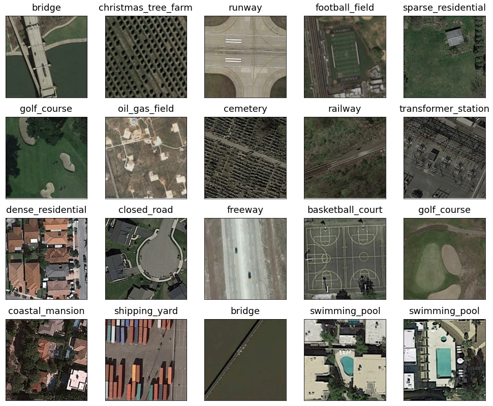
Model \Metric Accuracy Macro Precision Weighted Precision Macro Recall Weighted Recall Macro F1 score Weighted F1 score Avg. time / epoch (sec.) Total time (sec.) Best epoch AlexNet 99.16 99.17 99.17 99.16 99.16 99.16 99.16 15.17 637 32 VGG16 99.42 99.43 99.43 99.42 99.42 99.42 99.42 37.74 1321 25 ResNet50 99.74 99.74 99.74 99.74 99.74 99.74 99.74 29.10 1193 31 RestNet152 99.49 99.49 99.49 99.49 99.49 99.49 99.49 62.94 1070 7 DenseNet161 99.74 99.74 99.74 99.74 99.74 99.74 99.74 68.87 3168 36 EfficientNetB0 99.54 99.54 99.54 99.54 99.54 99.54 99.54 25.86 569 12 ConvNeXt 99.67 99.67 99.67 99.67 99.67 99.67 99.67 45.93 1378 20 Vision Transformer 99.65 99.66 99.66 99.65 99.65 99.65 99.65 48.50 1067 12 MLP Mixer 99.70 99.71 99.71 99.70 99.70 99.70 99.70 33.80 1521 35 Swin Transformer 99.69 99.69 99.69 99.69 99.69 99.69 99.69 138.65 2357 7
| Model \Metric |
Accuracy |
Macro Precision |
Weighted Precision |
Macro Recall |
Weighted Recall |
Macro F1 score |
Weighted F1 score |
Avg. time / epoch (sec.) |
Total time (sec.) |
Best epoch |
|---|---|---|---|---|---|---|---|---|---|---|
| AlexNet | 97.83 | 97.83 | 97.83 | 97.83 | 97.83 | 97.82 | 97.82 | 13.75 | 1141 | 68 |
| VGG16 | 97.91 | 97.93 | 97.93 | 97.91 | 97.91 | 97.91 | 97.91 | 37.47 | 2061 | 40 |
| ResNet50 | 99.06 | 99.07 | 99.07 | 99.06 | 99.06 | 99.06 | 99.06 | 35.65 | 3030 | 70 |
| RestNet152 | 98.88 | 98.89 | 98.89 | 98.88 | 98.88 | 98.88 | 98.88 | 69.05 | 6905 | 88 |
| DenseNet161 | 99.24 | 99.25 | 99.25 | 99.24 | 99.24 | 99.24 | 99.24 | 71.08 | 5260 | 59 |
| EfficientNetB0 | 98.83 | 98.84 | 98.84 | 98.83 | 98.83 | 98.83 | 98.83 | 27.54 | 2286 | 68 |
| ConvNeXt | 97.83 | 97.83 | 97.83 | 97.83 | 97.83 | 97.82 | 97.82 | 45.06 | 4326 | 81 |
| Vision Transformer | 96.69 | 96.69 | 96.69 | 96.69 | 96.69 | 96.68 | 96.68 | 49.05 | 3237 | 51 |
| MLP Mixer | 98.83 | 98.84 | 98.84 | 98.83 | 98.83 | 98.83 | 98.83 | 34.54 | 2038 | 44 |
| Swin Transformer | 98.52 | 98.53 | 98.53 | 98.52 | 98.52 | 98.52 | 98.52 | 138.59 | 12612 | 76 |
| Label | Precision | Recall | F1 score |
|---|---|---|---|
| airplane | 100.00 | 100.00 | 100.00 |
| baseball field | 100.00 | 100.00 | 100.00 |
| basketball court | 99.37 | 98.75 | 99.06 |
| beach | 100.00 | 100.00 | 100.00 |
| bridge | 98.77 | 100.00 | 99.38 |
| cemetery | 100.00 | 100.00 | 100.00 |
| chaparral | 100.00 | 100.00 | 100.00 |
| christmas tree farm | 100.00 | 100.00 | 100.00 |
| closed_road | 99.38 | 100.00 | 99.69 |
| coastal_mansion | 98.73 | 97.50 | 98.11 |
| crosswalk | 100.00 | 100.00 | 100.00 |
| dense_residential | 100.00 | 100.00 | 100.00 |
| ferry terminal | 100.00 | 98.75 | 99.37 |
| football field | 100.00 | 100.00 | 100.00 |
| forest | 100.00 | 100.00 | 100.00 |
| freeway | 100.00 | 100.00 | 100.00 |
| golf course | 100.00 | 100.00 | 100.00 |
| harbor | 100.00 | 100.00 | 100.00 |
| intersection | 99.38 | 100.00 | 99.69 |
| mobile home park | 100.00 | 100.00 | 100.00 |
| nursing home | 100.00 | 99.38 | 99.69 |
| oil gas field | 100.00 | 100.00 | 100.00 |
| oil well | 100.00 | 100.00 | 100.00 |
| overpass | 100.00 | 100.00 | 100.00 |
| parking lot | 100.00 | 100.00 | 100.00 |
| parking space | 100.00 | 100.00 | 100.00 |
| railway | 100.00 | 100.00 | 100.00 |
| river | 100.00 | 100.00 | 100.00 |
| runway | 100.00 | 99.38 | 99.69 |
| runway marking | 99.38 | 100.00 | 99.69 |
| shipping yard | 100.00 | 100.00 | 100.00 |
| solar panel | 100.00 | 100.00 | 100.00 |
| sparse residential | 96.91 | 98.13 | 97.52 |
| storage tank | 99.38 | 99.38 | 99.38 |
| swimming pool | 100.00 | 100.00 | 100.00 |
| tennis court | 100.00 | 99.38 | 99.69 |
| transformer station | 99.38 | 100.00 | 99.69 |
| wastewater treatment plant | 99.38 | 99.38 | 99.38 |

D.6 Resisc45
RESISC45 [8] dataset is a publicly available benchmark for Remote Sensing Image Scene Classification (RESISC), created by Northwestern Polytechnical University (NWPU). This dataset contains 31500 images, covering 45 scene classes with 700 images in each class. The 45 scene classes are as follows: airplane, airport, baseball diamond, basketball court, beach, bridge, chaparral, church, circular farmland, cloud, commercial area, dense residential, desert, forest, freeway, golf course, ground track field, harbor, industrial area, intersection, island, lake, meadow, medium residential, mobile home park, mountain, overpass, palace, parking lot, railway, railway station, rectangular farmland, river, roundabout, runway, sea ice, ship, snowberg, sparse residential, stadium, storage tank, tennis court, terrace, thermal power station, and wetland. Accordingly, these classes contain a variety of spatial patterns, some homogeneous with respect to texture, some homogeneous with respect to color, others not homogeneous at all.
The images are with a size of 256x256 pixels in the RGB color space. The spatial resolution varies from about 30m to 0.2m per pixel for most of the scene classes except for the classes of island, lake, mountain, and snowberg that have lower spatial resolutions. The 31500 images cover more than 100 countries and regions all over the world, including developing, transition, and highly developed economies (Figure 16). Our generated train, test and validation splits distribution is show on Figure 17.
Detailed results for all pre-trained models are shown on Table 17 and for all the models learned from scratch are presented on Table 18. The best performing model is the pre-trained Vision Transformer model. The results on a class level are show on Table 19 along with a confusion matrix on Figure 18.

Model \Metric Accuracy Macro Precision Weighted Precision Macro Recall Weighted Recall Macro F1 score Weighted F1 score Avg. time / epoch (sec.) Total time (sec.) Best epoch AlexNet 90.49 90.56 90.56 90.49 90.49 90.49 90.49 12.03 385 22 VGG16 93.90 93.91 93.91 93.90 93.90 93.89 93.89 39.87 1196 20 ResNet50 96.46 96.50 96.50 96.46 96.46 96.46 96.46 30.61 1163 28 RestNet152 96.54 96.57 96.57 96.54 96.54 96.54 96.54 65.11 2409 27 DenseNet161 96.51 96.53 96.53 96.51 96.51 96.51 96.51 72.05 3098 33 EfficientNetB0 94.87 94.93 94.93 94.87 94.87 94.88 94.88 27.12 678 15 ConvNeXt 96.27 96.28 96.28 96.27 96.27 96.26 96.26 46.79 1778 28 Vision Transformer 97.08 97.10 97.10 97.08 97.08 97.07 97.07 51.19 2713 43 MLP Mixer 95.95 95.99 95.99 95.95 95.95 95.96 95.96 35.62 1033 19 Swin Transformer 96.59 96.60 96.60 96.59 96.59 96.58 96.58 143.57 4020 18
| Model \Metric |
Accuracy |
Macro Precision |
Weighted Precision |
Macro Recall |
Weighted Recall |
Macro F1 score |
Weighted F1 score |
Avg. time / epoch (sec.) |
Total time (sec.) |
Best epoch |
|---|---|---|---|---|---|---|---|---|---|---|
| AlexNet | 82.16 | 82.29 | 82.29 | 82.16 | 82.16 | 82.10 | 82.10 | 10.91 | 633 | 43 |
| VGG16 | 83.89 | 84.00 | 84.00 | 83.89 | 83.89 | 83.84 | 83.84 | 38.37 | 2993 | 63 |
| ResNet50 | 92.33 | 92.40 | 92.40 | 92.33 | 92.33 | 92.33 | 92.33 | 31.31 | 1941 | 47 |
| RestNet152 | 90.68 | 90.79 | 90.79 | 90.68 | 90.68 | 90.69 | 90.69 | 64.83 | 4084 | 48 |
| DenseNet161 | 93.46 | 93.50 | 93.50 | 93.46 | 93.46 | 93.46 | 93.46 | 71.22 | 5484 | 62 |
| EfficientNetB0 | 91.37 | 91.47 | 91.47 | 91.37 | 91.37 | 91.38 | 91.38 | 27.66 | 2102 | 61 |
| ConvNeXt | 85.94 | 86.30 | 86.30 | 85.94 | 85.94 | 86.05 | 86.05 | 46.51 | 2279 | 34 |
| Vision Transformer | 81.02 | 81.18 | 81.18 | 81.02 | 81.02 | 80.98 | 80.98 | 50.21 | 2611 | 37 |
| MLP Mixer | 69.41 | 69.67 | 69.67 | 69.41 | 69.41 | 69.22 | 69.22 | 35.69 | 1285 | 21 |
| Swin Transformer | 88.73 | 88.82 | 88.82 | 88.73 | 88.73 | 88.71 | 88.71 | 144.87 | 14487 | 85 |
| Label | Precision | Recall | F1 score |
|---|---|---|---|
| airplane | 99.28 | 98.57 | 98.92 |
| airport | 95.89 | 100.00 | 97.90 |
| baseball_diamond | 97.89 | 99.29 | 98.58 |
| basketball_court | 97.22 | 100.00 | 98.59 |
| beach | 98.59 | 100.00 | 99.29 |
| bridge | 97.87 | 98.57 | 98.22 |
| chaparral | 97.90 | 100.00 | 98.94 |
| church | 90.85 | 92.14 | 91.49 |
| circular_farmland | 98.59 | 100.00 | 99.29 |
| cloud | 100.00 | 99.29 | 99.64 |
| commercial_area | 95.07 | 96.43 | 95.74 |
| dense_residential | 94.20 | 92.86 | 93.53 |
| desert | 97.86 | 97.86 | 97.86 |
| forest | 97.79 | 95.00 | 96.38 |
| freeway | 99.27 | 97.14 | 98.19 |
| golf_course | 98.58 | 99.29 | 98.93 |
| ground_track_field | 100.00 | 99.29 | 99.64 |
| harbor | 100.00 | 100.00 | 100.00 |
| industrial_area | 94.96 | 94.29 | 94.62 |
| intersection | 97.86 | 97.86 | 97.86 |
| island | 98.59 | 100.00 | 99.29 |
| lake | 93.75 | 96.43 | 95.07 |
| meadow | 95.00 | 95.00 | 95.00 |
| medium_residential | 91.61 | 93.57 | 92.58 |
| mobile_home_park | 97.22 | 100.00 | 98.59 |
| mountain | 95.74 | 96.43 | 96.09 |
| overpass | 99.25 | 94.29 | 96.70 |
| palace | 91.91 | 89.29 | 90.58 |
| parking_lot | 99.28 | 98.57 | 98.92 |
| railway | 93.84 | 97.86 | 95.80 |
| railway_station | 96.30 | 92.86 | 94.55 |
| rectangular_farmland | 91.95 | 97.86 | 94.81 |
| river | 99.24 | 92.86 | 95.94 |
| roundabout | 99.29 | 100.00 | 99.64 |
| runway | 100.00 | 95.71 | 97.81 |
| sea_ice | 100.00 | 98.57 | 99.28 |
| ship | 97.22 | 100.00 | 98.59 |
| snowberg | 98.59 | 100.00 | 99.29 |
| sparse_residential | 96.43 | 96.43 | 96.43 |
| stadium | 97.90 | 100.00 | 98.94 |
| storage_tank | 98.56 | 97.86 | 98.21 |
| tennis_court | 98.54 | 96.43 | 97.47 |
| terrace | 96.21 | 90.71 | 93.38 |
| thermal_power_station | 96.45 | 97.14 | 96.80 |
| wetland | 97.01 | 92.86 | 94.89 |

D.7 RSI-CB256
RSI-CB256 [45] is a large scale remote sensing image classification benchmark via crowdsource data such as Open Street Map (OSM) data, ground objects in remote sensing images etc. It contains 35 categories and more than 24000 images with a size of 256x256 pixels (Figure 19). A strict object category system according to the national standard of land-use classification in China and the hierarchical grading mechanism of ImageNet-1K has been established. Using crowd-source data as a supervisor facilitates machine self-learning through the Internet. The class distribution of the train, test and validation splits is presented in Figure 20.
Detailed results for all pre-trained models are shown on Table 20 and for all the models learned from scratch are presented on Table 21. The best performing model is the pre-trained ResNet152 model. The results on a class level are show on Table 22 along with a confusion matrix on Figure 21.

Model \Metric Accuracy Macro Precision Weighted Precision Macro Recall Weighted Recall Macro F1 score Weighted F1 score Avg. time / epoch (sec.) Total time (sec.) Best epoch AlexNet 99.35 99.13 99.36 99.06 99.35 99.09 99.35 34.84 1568 35 VGG16 99.05 98.93 99.07 98.75 99.05 98.83 99.05 34.04 885 16 ResNet50 99.68 99.53 99.68 99.54 99.68 99.53 99.68 33.69 1078 22 RestNet152 99.86 99.85 99.86 99.82 99.86 99.83 99.86 51.90 1609 21 DenseNet161 99.74 99.68 99.74 99.64 99.74 99.66 99.74 56.60 2717 38 EfficientNetB0 99.72 99.63 99.72 99.65 99.72 99.64 99.72 33.50 1340 30 ConvNeXt 99.60 99.50 99.60 99.55 99.60 99.52 99.60 40.35 1977 39 Vision Transformer 99.76 99.75 99.76 99.71 99.76 99.73 99.76 41.18 1400 24 MLP Mixer 99.66 99.54 99.66 99.61 99.66 99.57 99.66 35.29 1235 25 Swin Transformer 99.68 99.54 99.68 99.62 99.68 99.57 99.68 113.14 4752 32
Model \Metric Accuracy Macro Precision Weighted Precision Macro Recall Weighted Recall Macro F1 score Weighted F1 score Avg. time / epoch (sec.) Total time (sec.) Best epoch AlexNet 97.35 96.55 97.39 96.54 97.35 96.51 97.35 34.99 2414 54 VGG16 98.83 98.51 98.84 98.36 98.83 98.43 98.83 34.90 2757 64 ResNet50 98.83 98.51 98.84 98.36 98.83 98.43 98.83 36.39 3166 72 RestNet152 99.15 98.98 99.15 98.81 99.15 98.89 99.15 51.86 4472 72 DenseNet161 99.13 98.80 99.13 98.71 99.13 98.75 99.13 56.75 4029 56 EfficientNetB0 99.11 98.85 99.12 98.91 99.11 98.87 99.11 26.50 2123 71 ConvNeXt 98.44 97.75 98.45 97.74 98.44 97.73 98.44 36.93 2622 56 Vision Transformer 98.12 97.52 98.13 97.12 98.12 97.31 98.12 41.08 3204 63 MLP Mixer 98.42 97.81 98.43 97.80 98.42 97.79 98.42 29.00 2900 86 Swin Transformer 99.09 98.83 99.09 98.70 99.09 98.76 99.09 113.60 7157 48
| Label | Precision | Recall | F1 score |
|---|---|---|---|
| airplane | 100.00 | 100.00 | 100.00 |
| airport_runway | 100.00 | 100.00 | 100.00 |
| artificial_grassland | 100.00 | 100.00 | 100.00 |
| avenue | 100.00 | 99.08 | 99.54 |
| bare_land | 98.30 | 100.00 | 99.14 |
| bridge | 98.95 | 100.00 | 99.47 |
| city_building | 100.00 | 100.00 | 100.00 |
| coastline | 100.00 | 98.91 | 99.45 |
| container | 100.00 | 99.24 | 99.62 |
| crossroads | 99.11 | 100.00 | 99.55 |
| dam | 100.00 | 100.00 | 100.00 |
| desert | 100.00 | 98.62 | 99.31 |
| dry_farm | 100.00 | 100.00 | 100.00 |
| forest | 100.00 | 100.00 | 100.00 |
| green_farmland | 100.00 | 100.00 | 100.00 |
| highway | 100.00 | 97.73 | 98.85 |
| hirst | 100.00 | 100.00 | 100.00 |
| lakeshore | 100.00 | 100.00 | 100.00 |
| mangrove | 100.00 | 100.00 | 100.00 |
| marina | 100.00 | 100.00 | 100.00 |
| mountain | 100.00 | 100.00 | 100.00 |
| parkinglot | 98.94 | 100.00 | 99.47 |
| pipeline | 100.00 | 100.00 | 100.00 |
| residents | 100.00 | 100.00 | 100.00 |
| river | 100.00 | 100.00 | 100.00 |
| river_protection_forest | 100.00 | 100.00 | 100.00 |
| sandbeach | 100.00 | 100.00 | 100.00 |
| sapling | 100.00 | 100.00 | 100.00 |
| sea | 99.52 | 100.00 | 99.76 |
| shrubwood | 100.00 | 100.00 | 100.00 |
| snow_mountain | 100.00 | 100.00 | 100.00 |
| sparse_forest | 100.00 | 100.00 | 100.00 |
| storage_room | 100.00 | 100.00 | 100.00 |
| stream | 100.00 | 100.00 | 100.00 |
| town | 100.00 | 100.00 | 100.00 |

D.8 RSSCN7
RSSCN7 [46] is a scene classification dataset. The images are obtained from Google Earth. This dataset was collected for academic research. It contains a total of 2800 remote sensing images, which are organized into 7 scene classes: grass land, forest, farm land, parking lot, residential region, industrial region, and river/lake (Figure 22). For each, class there are 400 RGB images that are cropped on four different scales with 100 images per scale. Each image has a 400x400 pixels size. The main challenge of this dataset is the scale variations of the images. The class distribution over the train, test and validation splits is presented on Figure 23.
Detailed results for all pre-trained models are shown on Table 23 and for all the models learned from scratch are presented on Table 24. The best performing model is the pre-trained Vision Transformer model. The results on a class level are show on Table 25 along with a confusion matrix on Figure 24.

Model \Metric Accuracy Macro Precision Weighted Precision Macro Recall Weighted Recall Macro F1 score Weighted F1 score Avg. time / epoch (sec.) Total time (sec.) Best epoch AlexNet 91.96 92.05 92.05 91.96 91.96 91.92 91.92 3.19 118 27 VGG16 93.93 93.95 93.95 93.93 93.93 93.90 93.90 4.68 159 24 ResNet50 95.00 95.08 95.08 95.00 95.00 94.99 94.99 3.90 121 21 RestNet152 95.00 95.07 95.07 95.00 95.00 95.01 95.01 7.09 241 24 DenseNet161 94.82 94.83 94.83 94.82 94.82 94.82 94.82 7.59 220 19 EfficientNetB0 95.54 95.56 95.56 95.54 95.54 95.54 95.54 3.79 163 33 ConvNeXt 94.64 94.76 94.76 94.64 94.64 94.61 94.61 5.23 183 25 Vision Transformer 95.89 95.95 95.95 95.89 95.89 95.91 95.91 5.54 227 31 MLP Mixer 95.18 95.23 95.23 95.18 95.18 95.17 95.17 4.30 86 10 Swin Transformer 95.18 95.23 95.23 95.18 95.18 95.18 95.18 13.42 416 21
Model \Metric Accuracy Macro Precision Weighted Precision Macro Recall Weighted Recall Macro F1 score Weighted F1 score Avg. time / epoch (sec.) Total time (sec.) Best epoch AlexNet 80.54 80.64 80.64 80.54 80.54 80.45 80.45 6.97 697 85 VGG16 81.61 81.50 81.50 81.61 81.61 81.41 81.41 6.74 526 63 ResNet50 82.68 82.65 82.65 82.68 82.68 82.41 82.41 3.76 316 69 RestNet152 82.68 82.65 82.65 82.68 82.68 82.41 82.41 6.90 407 44 DenseNet161 87.32 87.55 87.55 87.32 87.32 87.38 87.38 8.50 595 55 EfficientNetB0 83.93 84.03 84.03 83.93 83.93 83.87 83.87 3.65 365 93 ConvNeXt 83.04 82.84 82.84 83.04 83.04 82.90 82.90 5.43 543 87 Vision Transformer 86.07 86.17 86.17 86.07 86.07 86.00 86.00 5.52 453 67 MLP Mixer 83.21 83.29 83.29 83.21 83.21 83.17 83.17 4.08 408 100 Swin Transformer 82.50 82.59 82.59 82.50 82.50 82.50 82.50 13.78 951 54
| Label | Precision | Recall | F1 score |
|---|---|---|---|
| farm_land | 97.40 | 93.75 | 95.54 |
| forest | 100.00 | 98.75 | 99.37 |
| grass_land | 91.57 | 95.00 | 93.25 |
| industrial_region | 92.59 | 93.75 | 93.17 |
| parking_lot | 94.94 | 93.75 | 94.34 |
| residential_region | 100.00 | 98.75 | 99.37 |
| river_lake | 95.12 | 97.50 | 96.30 |

D.9 SAT6
SAT-6 [47] consists of a total of 405000 image patches each of size 28x28 and covering 6 land cover classes - barren land, trees, grassland, roads, buildings and water bodies (Figure 25). The authors of the dataset selected 324000 images for the training dataset and 81000 were selected as testing dataset. Additionally we have selected 20% of the images from the train dataset to create the validation split. The training and test datasets were selected from disjoint National Agriculture Imagery Program (NAIP) tiles. The specifications for the various land cover classes of SAT-6 were adopted from those used in the National Land Cover Data (NLCD) algorithm. The class distribution of the train, test and validation splits is presented on Figure 25.
Detailed results for all pre-trained models are shown on Table 26 and for all the models learned from scratch are presented on Table 27. All pre-trained model obtained excellent result on the dataset with ResNet50, ResNet152, DenseNet161, ConvNeXt, Vision Transformer, MLPMixer and Swin Transformer achieving 100 % accuracy. The results on a class level are show on Table 28 along with a confusion matrix on Figure 27 for the DenseNet161 model.

Model \Metric Accuracy Macro Precision Weighted Precision Macro Recall Weighted Recall Macro F1 score Weighted F1 score Avg. time / epoch (sec.) Total time (sec.) Best epoch AlexNet 99.98 99.98 99.98 99.97 99.98 99.97 99.98 92.48 5364 48 VGG16 99.99 99.99 99.99 99.99 99.99 99.99 99.99 550.04 29702 44 ResNet50 100.00 100.00 100.00 100.00 100.00 100.00 100.00 410.33 37340 81 RestNet152 100.00 100.00 100.00 100.00 100.00 100.00 100.00 872.87 61974 61 DenseNet161 100.00 100.00 100.00 100.00 100.00 100.00 100.00 970.39 55312 47 EfficientNetB0 99.99 99.99 99.99 99.99 99.99 99.99 99.99 363.00 8712 14 ConvNeXt 100.00 100.00 100.00 99.99 100.00 100.00 100.00 630.78 42262 57 Vision Transformer 100.00 100.00 100.00 100.00 100.00 100.00 100.00 692.50 42935 52 MLP Mixer 100.00 100.00 100.00 100.00 100.00 100.00 100.00 476.34 15243 22 Swin Transformer 100.00 100.00 100.00 100.00 100.00 100.00 100.00 2,003.62 106192 43
Model \Metric Accuracy Macro Precision Weighted Precision Macro Recall Weighted Recall Macro F1 score Weighted F1 score Avg. time / epoch (sec.) Total time (sec.) Best epoch AlexNet 99.27 98.67 99.27 98.65 99.27 98.66 99.27 107.26 10726 98 VGG16 99.56 99.42 99.56 99.42 99.56 99.42 99.56 579.10 57910 98 ResNet50 100.00 100.00 100.00 100.00 100.00 100.00 100.00 457.04 45704 99 RestNet152 100.00 100.00 100.00 100.00 100.00 100.00 100.00 987.21 98721 94 DenseNet161 100.00 100.00 100.00 100.00 100.00 100.00 100.00 956.03 95603 85 EfficientNetB0 100.00 100.00 100.00 100.00 100.00 100.00 100.00 420.37 42037 95 ConvNeXt 100.00 100.00 100.00 100.00 100.00 100.00 100.00 627.69 62769 97 Vision Transformer 99.99 99.98 99.99 99.98 99.99 99.98 99.99 687.12 61841 75 MLP Mixer 99.98 99.98 99.98 99.96 99.98 99.97 99.98 479.37 47937 95 Swin Transformer 99.98 99.96 99.98 99.97 99.98 99.97 99.98 1,973.44 197344 99
| Label | Precision | Recall | F1 score |
|---|---|---|---|
| buildings | 100.00 | 100.00 | 100.00 |
| barren land | 100.00 | 100.00 | 100.00 |
| trees | 100.00 | 100.00 | 100.00 |
| grassland | 100.00 | 100.00 | 100.00 |
| roads | 100.00 | 100.00 | 100.00 |
| water bodies | 100.00 | 100.00 | 100.00 |

D.10 Siri-Whu
The SIRI-WHU [48] is a scene classification dataset comprised of 2400 images organized into 12 classes. Each class contains 200 images with a 2m spatial resolution and a size of 200×200 pixels (Figure 28). It was collected from Google Earth (Google Inc.) by the Intelligent Data Extraction and Analysis of Remote Sensing (RS_IDEA) Group in Wuhan University. The 12 land-use classes contain agriculture, commercial, harbor, idle land, industrial, meadow, overpass, park, pond, residential, river, and water. This dataset mainly covers urban areas in China, which means it lack diversity and is less challenging. The class distribution is presented on Figure 29.
Detailed results for all pre-trained models are shown on Table 29 and for all the models learned from scratch are presented on Table 30. The best performing model is the pre-trained ResNet152 model. The results on a class level are show on Table 31 along with a confusion matrix on Figure 30.

Model \Metric Accuracy Macro Precision Weighted Precision Macro Recall Weighted Recall Macro F1 score Weighted F1 score Avg. time / epoch (sec.) Total time (sec.) Best epoch AlexNet 92.29 92.64 92.64 92.29 92.29 92.31 92.31 4.28 197 36 VGG16 93.96 94.08 94.08 93.96 93.96 93.96 93.96 4.98 214 33 ResNet50 95.00 95.12 95.12 95.00 95.00 95.01 95.01 4.66 191 31 RestNet152 96.25 96.27 96.27 96.25 96.25 96.24 96.24 6.65 226 24 DenseNet161 95.63 95.64 95.64 95.63 95.63 95.61 95.61 7.30 365 40 EfficientNetB0 95.00 95.09 95.09 95.00 95.00 95.01 95.01 4.57 329 62 ConvNeXt 96.25 96.34 96.34 96.25 96.25 96.24 96.24 5.64 203 26 Vision Transformer 95.63 95.73 95.73 95.63 95.62 95.63 95.63 5.37 322 50 MLP Mixer 95.21 95.36 95.36 95.21 95.21 95.23 95.23 4.55 150 23 Swin Transformer 95.63 95.60 95.60 95.63 95.62 95.57 95.57 11.87 534 35
Model \Metric Accuracy Macro Precision Weighted Precision Macro Recall Weighted Recall Macro F1 score Weighted F1 score Avg. time / epoch (sec.) Total time (sec.) Best epoch AlexNet 83.75 83.83 83.83 83.75 83.75 83.66 83.66 3.54 326 77 VGG16 84.79 85.05 85.05 84.79 84.79 84.70 84.70 7.32 732 93 ResNet50 88.96 89.14 89.14 88.96 88.96 88.94 88.94 3.81 305 65 RestNet152 88.75 88.67 88.67 88.75 88.75 88.62 88.62 6.54 608 78 DenseNet161 86.67 87.38 87.38 86.67 86.67 86.56 86.56 7.49 749 94 EfficientNetB0 86.04 86.23 86.23 86.04 86.04 85.94 85.94 3.61 238 51 ConvNeXt 84.17 84.32 84.32 84.17 84.17 84.09 84.09 11.99 1007 69 Vision Transformer 86.25 86.31 86.31 86.25 86.25 86.14 86.14 5.08 503 84 MLP Mixer 82.50 82.40 82.40 82.50 82.50 82.34 82.34 3.92 392 98 Swin Transformer 85.83 86.02 86.02 85.83 85.83 85.62 85.62 12.10 1113 77
| Label | Precision | Recall | F1 score |
|---|---|---|---|
| agriculture | 100.00 | 100.00 | 100.00 |
| commercial | 100.00 | 97.50 | 98.73 |
| harbor | 90.48 | 95.00 | 92.68 |
| idle_land | 97.50 | 97.50 | 97.50 |
| industrial | 100.00 | 97.50 | 98.73 |
| meadow | 92.11 | 87.50 | 89.74 |
| overpass | 95.24 | 100.00 | 97.56 |
| park | 92.31 | 90.00 | 91.14 |
| pond | 100.00 | 100.00 | 100.00 |
| residential | 97.56 | 100.00 | 98.77 |
| river | 92.50 | 92.50 | 92.50 |
| water | 97.50 | 97.50 | 97.50 |

D.11 CLRS
This dataset [49] is a database designed for the task named Continual/Lifelong learning for remote sensing image scene classification. The proposed CLRS dataset consists of 15000 remote sensing images divided into 25 scene classes covering over 100 countries (Figure 31). The images have a spatial resolution between 0.26 8.85 meters. The data is acquired from multiple sources such as: Google Earth, Bing Map, Google Map, and Tianditu. The class distribution of the train, test and validation splits is presented on Figure 32.
Detailed results for all pre-trained models are shown on Table 32 and for all the models learned from scratch are presented on Table 33. The best performing model is the pre-trained Vision Transformer model. The results on a class level are show on Table 34 along with a confusion matrix on Figure 33.

Model \Metric Accuracy Macro Precision Weighted Precision Macro Recall Weighted Recall Macro F1 score Weighted F1 score Avg. time / epoch (sec.) Total time (sec.) Best epoch AlexNet 84.10 84.19 84.19 84.10 84.10 84.03 84.03 20.48 635 21 VGG16 89.90 89.97 89.97 89.90 89.90 89.90 89.90 20.23 607 20 ResNet50 91.57 91.67 91.67 91.57 91.57 91.58 91.58 18.60 279 15 RestNet152 91.90 91.99 91.99 91.90 91.90 91.91 91.91 31.96 799 15 DenseNet161 92.20 92.29 92.29 92.20 92.20 92.20 92.20 35.46 993 18 EfficientNetB0 90.50 90.61 90.61 90.50 90.50 90.49 90.49 19.73 513 16 ConvNeXt 91.10 91.29 91.29 91.10 91.10 91.12 91.12 23.62 496 11 Vision Transformer 93.20 93.29 93.29 93.20 93.20 93.22 93.22 25.32 785 21 MLP Mixer 90.10 90.21 90.21 90.10 90.10 90.05 90.05 19.75 316 6 Swin Transformer 92.53 92.53 92.53 92.53 92.53 92.51 92.51 68.93 1861 17
Model \Metric Accuracy Macro Precision Weighted Precision Macro Recall Weighted Recall Macro F1 score Weighted F1 score Avg. time / epoch (sec.) Total time (sec.) Best epoch AlexNet 71.40 71.59 71.59 71.40 71.40 71.33 71.33 20.35 2035 92 VGG16 76.07 76.20 76.20 76.07 76.07 76.00 76.00 19.33 1450 60 ResNet50 85.57 85.72 85.72 85.57 85.57 85.57 85.57 19.43 1788 77 RestNet152 82.30 82.47 82.47 82.30 82.30 82.19 82.19 32.05 2373 60 DenseNet161 86.17 86.29 86.29 86.17 86.17 86.18 86.18 35.81 2757 62 EfficientNetB0 82.27 82.55 82.55 82.27 82.27 82.31 82.31 20.71 1512 58 ConvNeXt 69.17 69.02 69.02 69.17 69.17 69.01 69.01 23.09 2309 96 Vision Transformer 65.47 66.41 66.41 65.47 65.47 65.49 65.49 24.96 1173 32 MLP Mixer 61.13 62.18 62.18 61.13 61.13 60.87 60.87 17.98 809 30 Swin Transformer 80.00 80.10 80.10 80.00 80.00 79.91 79.91 69.19 5535 65
| Label | Precision | Recall | F1 score |
|---|---|---|---|
| airport | 97.48 | 96.67 | 97.07 |
| bare-land | 92.00 | 95.83 | 93.88 |
| beach | 99.15 | 97.50 | 98.32 |
| bridge | 90.91 | 91.67 | 91.29 |
| commercial | 79.84 | 85.83 | 82.73 |
| desert | 97.50 | 97.50 | 97.50 |
| farmland | 93.70 | 99.17 | 96.36 |
| forest | 100.00 | 100.00 | 100.00 |
| golf-course | 94.96 | 94.17 | 94.56 |
| highway | 92.11 | 87.50 | 89.74 |
| industrial | 88.79 | 85.83 | 87.29 |
| meadow | 96.72 | 98.33 | 97.52 |
| mountain | 99.15 | 97.50 | 98.32 |
| overpass | 89.68 | 94.17 | 91.87 |
| park | 85.60 | 89.17 | 87.35 |
| parking | 98.25 | 93.33 | 95.73 |
| playground | 95.04 | 95.83 | 95.44 |
| port | 94.74 | 90.00 | 92.31 |
| railway | 86.29 | 89.17 | 87.70 |
| railway-station | 88.79 | 85.83 | 87.29 |
| residential | 90.68 | 89.17 | 89.92 |
| river | 90.32 | 93.33 | 91.80 |
| runway | 98.33 | 98.33 | 98.33 |
| stadium | 95.61 | 90.83 | 93.16 |
| storage-tank | 96.55 | 93.33 | 94.92 |

D.12 RSD46-WHU
RSD46-WHU is a large-scale open dataset for scene classification in remote sensing images. The dataset is manually collected from Google Earth and Tianditu. The ground resolution of most classes is 0.5m, and the others are about 2m. There are 500-3000 images in each class. The RSD46-WHU dataset contains around 117000 images with 46 classes (Figure 34). The image are not evenly distributed between classes and each class contains between 428 to 3000 images. The dataset comes with predefined train and test splits. For creating the validation split we used 20% of the images from the train split. The class distribution of the different splits is presented on Figure 35.
Detailed results for all pre-trained models are shown on Table 35 and for all the models learned from scratch are presented on Table 36. The best performing model is the pre-trained DenseNet161 model. The results on a class level are show on Table 37 along with a confusion matrix on Figure 36.

Model \Metric Accuracy Macro Precision Weighted Precision Macro Recall Weighted Recall Macro F1 score Weighted F1 score Avg. time / epoch (sec.) Total time (sec.) Best epoch AlexNet 90.65 90.43 90.61 90.35 90.65 90.36 90.61 58.03 2031 25 VGG16 92.42 92.30 92.38 92.25 92.42 92.22 92.37 158.32 4433 18 ResNet50 94.16 94.07 94.15 94.18 94.16 94.11 94.14 123.27 3205 16 RestNet152 94.40 94.33 94.40 94.41 94.40 94.36 94.39 269.45 7814 19 DenseNet161 94.51 94.36 94.49 94.41 94.51 94.36 94.48 297.70 6847 13 EfficientNetB0 93.39 93.20 93.38 93.39 93.39 93.26 93.35 111.55 2231 10 ConvNeXt 93.63 93.61 93.67 93.47 93.63 93.48 93.60 196.20 3924 10 Vision Transformer 94.24 94.38 94.23 94.08 94.24 94.16 94.20 210.37 3997 9 MLP Mixer 93.67 93.77 93.69 93.47 93.67 93.55 93.65 148.25 3558 14 Swin Transformer 93.54 93.48 93.62 93.62 93.54 93.50 93.52 599.42 11389 9
Model \Metric Accuracy Macro Precision Weighted Precision Macro Recall Weighted Recall Macro F1 score Weighted F1 score Avg. time / epoch (sec.) Total time (sec.) Best epoch AlexNet 86.03 85.83 86.03 85.67 86.03 85.71 85.99 58.84 3707 48 VGG16 88.62 88.37 88.56 88.37 88.62 88.32 88.55 162.89 8796 39 ResNet50 90.55 90.40 90.53 90.26 90.55 90.30 90.52 127.53 8672 53 RestNet152 89.94 89.84 89.99 89.77 89.94 89.78 89.95 272.70 19907 58 DenseNet161 92.21 92.11 92.23 92.03 92.21 92.06 92.21 301.16 15318 36 EfficientNetB0 90.61 90.57 90.61 90.25 90.61 90.37 90.58 113.93 6446 40 ConvNeXt 88.69 88.66 88.67 88.33 88.69 88.46 88.66 194.93 11891 46 Vision Transformer 86.47 86.22 86.45 85.94 86.47 86.02 86.42 211.93 9325 29 MLP Mixer 81.25 81.56 81.59 80.11 81.25 80.51 81.19 148.42 4149 12 Swin Transformer 91.81 91.50 91.79 91.48 91.81 91.47 91.79 588.25 41766 56
| Label | Precision | Recall | F1 score |
|---|---|---|---|
| Airplane | 99.56 | 99.78 | 99.67 |
| Airport | 98.39 | 99.19 | 98.79 |
| Artificial dense forest land | 87.11 | 86.90 | 87.01 |
| Artificial sparse forest land | 87.06 | 82.55 | 84.75 |
| Bare land | 94.12 | 96.00 | 95.05 |
| Basketball court | 90.37 | 92.39 | 91.37 |
| Blue structured factory building | 96.57 | 97.83 | 97.19 |
| Building | 82.44 | 83.40 | 82.92 |
| Construction site | 82.11 | 79.43 | 80.75 |
| Cross river bridge | 99.70 | 99.70 | 99.70 |
| Crossroads | 97.74 | 98.70 | 98.22 |
| Dense tall building | 94.35 | 94.35 | 94.35 |
| Dock | 98.94 | 98.73 | 98.83 |
| Fish pond | 97.52 | 97.93 | 97.72 |
| Footbridge | 99.49 | 99.24 | 99.36 |
| Graff | 98.37 | 93.79 | 96.03 |
| Grassland | 95.07 | 95.52 | 95.29 |
| Low scattered building | 96.15 | 97.49 | 96.82 |
| Lrregular farmland | 97.68 | 98.51 | 98.09 |
| Medium density scattered building | 76.98 | 68.15 | 72.30 |
| Medium density structured building | 89.58 | 92.11 | 90.82 |
| Natural dense forest land | 95.40 | 96.89 | 96.14 |
| Natural sparse forest land | 93.16 | 97.98 | 95.51 |
| Oiltank | 90.66 | 96.68 | 93.57 |
| Overpass | 99.19 | 98.13 | 98.66 |
| Parking lot | 96.49 | 96.07 | 96.28 |
| Plasticgreenhouse | 100.00 | 99.34 | 99.67 |
| Playground | 96.85 | 95.84 | 96.34 |
| Railway | 99.14 | 99.14 | 99.14 |
| Red structured factory building | 97.78 | 98.66 | 98.22 |
| Refinery | 92.84 | 87.72 | 90.21 |
| Regular farmland | 95.20 | 94.80 | 95.00 |
| Scattered blue roof factory building | 94.44 | 96.72 | 95.57 |
| Scattered red roof factory building | 93.28 | 97.73 | 95.45 |
| Sewage plant-type-one | 95.06 | 96.25 | 95.65 |
| Sewage plant-type-two | 88.73 | 98.44 | 93.33 |
| Ship | 99.56 | 99.33 | 99.45 |
| Solar power station | 99.78 | 99.78 | 99.78 |
| Sparse residential area | 91.42 | 88.14 | 89.75 |
| Square | 94.52 | 97.38 | 95.93 |
| Steelsmelter | 90.48 | 90.89 | 90.68 |
| Storage land | 99.03 | 96.52 | 97.76 |
| Tennis court | 95.93 | 91.38 | 93.60 |
| Thermal power plant | 88.95 | 85.19 | 87.03 |
| Vegetable plot | 94.12 | 92.59 | 93.35 |
| Water | 99.02 | 99.51 | 99.26 |

D.13 Brazilian Coffee Scenes
The Brazilian Coffee Scenes dataset [52] consists of only two classes: coffee and non-coffee class. Each class has 1438 images with 64x64 pixels cropped from SPOT satellite images over four counties in the state of Minas Gerais, Brazil: Arceburgo, Guaranesia, Guaxupe, and Monte Santo (Figure 37). The images in the dataset are in green, red and near-infrared spectral bands, since these are most useful and representative for distinguishing vegetation areas. The dataset is manually annotated by agricultural researchers. Images which contain coffee pixels in at least 85% of the image were assigned to the coffee class. Image with less than 10% of coffee pixels are assigned to the non-coffee class. The number of classes and the degree to which the data is tailored, should make this less challenging dataset. The class distribution is presented on Figure 38.
Detailed results for all pre-trained models are shown on Table 38 and for all the models learned from scratch are presented on Table 39. The best performing model is the pre-trained Swin Transformer model. The results on a class level are show on Table 40 along with a confusion matrix on Figure 39.

Model \Metric Accuracy Macro Precision Weighted Precision Macro Recall Weighted Recall Macro F1 score Weighted F1 score Avg. time / epoch (sec.) Total time (sec.) Best epoch AlexNet 89.58 89.59 89.59 89.58 89.58 89.58 89.58 1.48 43 19 VGG16 90.97 91.00 91.00 90.97 90.97 90.97 90.97 4.17 121 19 ResNet50 92.01 92.06 92.06 92.01 92.01 92.01 92.01 3.45 76 12 RestNet152 92.36 92.37 92.37 92.36 92.36 92.36 92.36 6.61 119 8 DenseNet161 92.71 92.81 92.81 92.71 92.71 92.70 92.70 7.33 176 14 EfficientNetB0 91.32 91.32 91.32 91.32 91.32 91.32 91.32 3.17 133 32 ConvNeXt 91.49 91.58 91.58 91.49 91.49 91.49 91.49 5.08 132 16 Vision Transformer 92.01 92.03 92.03 92.01 92.01 92.01 92.01 5.07 76 5 MLP Mixer 93.06 93.07 93.07 93.06 93.06 93.05 93.05 3.94 67 7 Swin Transformer 93.40 93.40 93.40 93.40 93.40 93.40 93.40 13.88 222 6
Model \Metric Accuracy Macro Precision Weighted Precision Macro Recall Weighted Recall Macro F1 score Weighted F1 score Avg. time / epoch (sec.) Total time (sec.) Best epoch AlexNet 89.41 89.62 89.62 89.41 89.41 89.40 89.40 1.53 115 60 VGG16 89.41 89.45 89.45 89.41 89.41 89.41 89.41 5.95 440 59 ResNet50 89.24 89.39 89.39 89.24 89.24 89.23 89.23 4.55 296 50 RestNet152 88.54 88.56 88.56 88.54 88.54 88.54 88.54 7.95 469 44 DenseNet161 90.80 90.80 90.80 90.80 90.80 90.80 90.80 7.31 373 36 EfficientNetB0 85.42 85.71 85.71 85.42 85.42 85.39 85.39 3.26 326 98 ConvNeXt 84.38 84.39 84.39 84.38 84.38 84.37 84.37 5.09 509 95 Vision Transformer 87.85 87.89 87.89 87.85 87.85 87.84 87.84 5.55 322 43 MLP Mixer 86.28 86.29 86.29 86.28 86.28 86.28 86.28 4.47 201 30 Swin Transformer 89.24 89.33 89.33 89.24 89.24 89.23 89.23 13.59 1169 71
| Label | Precision | Recall | F1 score |
|---|---|---|---|
| coffee | 93.10 | 93.75 | 93.43 |
| noncoffee | 93.71 | 93.06 | 93.38 |

D.14 Optimal 31
The Optimal 31 dataset [51] is for remote sensing image scene classification. The dataset contains 31 classes, each class contains 60 images with a size of 256×256 pixels. Totaling 1860 aerial RGB images (Figure 40). These classes include: airplane, airport, basketball court, baseball field, bridge, beach, bushes, crossroads, church, round farmland, business district, desert, harbor, dense houses, factory, forest, freeway, golf field, island, lake, meadow, medium houses, mountain, mobile house area, overpass, playground, parking lot, roundabout, runway, railway, and square farmland. It is considered challenging due to small number of images dispersed across many classes. We have generated train, test and validation spits for our study and their class distribution is presented on Figure 41.
Detailed results for all pre-trained models are shown on Table 41 and for all the models learned from scratch are presented on Table 42. The best performing model is the pre-trained Vision Transformer model. The results on a class level are show on Table 43 along with a confusion matrix on Figure 42.

Model \Metric Accuracy Macro Precision Weighted Precision Macro Recall Weighted Recall Macro F1 score Weighted F1 score Avg. time / epoch (sec.) Total time (sec.) Best epoch AlexNet 80.91 81.90 81.90 80.91 80.91 80.74 80.74 1.10 45 31 VGG16 88.71 89.58 89.58 88.71 88.71 88.79 88.79 2.97 95 22 ResNet50 92.20 92.85 92.85 92.20 92.20 92.25 92.25 2.58 129 40 RestNet152 92.47 92.99 92.99 92.47 92.47 92.47 92.47 4.62 217 37 DenseNet161 94.35 94.92 94.92 94.35 94.35 94.43 94.43 5.02 306 51 EfficientNetB0 91.67 92.04 92.04 91.67 91.67 91.60 91.60 2.25 187 73 ConvNeXt 93.01 93.33 93.33 93.01 93.01 92.99 92.99 3.50 203 48 Vision Transformer 94.62 94.85 94.85 94.62 94.62 94.56 94.56 3.71 126 24 MLP Mixer 92.74 93.17 93.17 92.74 92.74 92.74 92.74 2.82 141 40 Swin Transformer 92.47 92.92 92.92 92.47 92.47 92.51 92.51 9.19 340 27
Model \Metric Accuracy Macro Precision Weighted Precision Macro Recall Weighted Recall Macro F1 score Weighted F1 score Avg. time / epoch (sec.) Total time (sec.) Best epoch AlexNet 55.11 55.61 55.61 55.11 55.11 54.24 54.24 1.23 101 67 VGG16 56.72 58.89 58.89 56.72 56.72 56.58 56.58 4.81 409 70 ResNet50 67.20 69.56 69.56 67.20 67.20 67.17 67.17 2.60 161 47 RestNet152 62.90 64.95 64.95 62.90 62.90 62.78 62.78 5.92 314 38 DenseNet161 71.24 72.01 72.01 71.24 71.24 70.65 70.65 5.16 330 49 EfficientNetB0 68.55 70.59 70.59 68.55 68.55 68.70 68.70 2.36 156 51 ConvNeXt 58.87 60.69 60.69 58.87 58.87 58.92 58.92 3.59 330 77 Vision Transformer 62.63 63.89 63.89 62.63 62.63 62.32 62.32 3.79 235 47 MLP Mixer 59.14 60.36 60.36 59.14 59.14 58.47 58.47 3.26 326 98 Swin Transformer 66.13 67.47 67.47 66.13 66.13 65.62 65.62 9.51 951 89
| Label | Precision | Recall | F1 score |
|---|---|---|---|
| airplane | 100.00 | 100.00 | 100.00 |
| airport | 100.00 | 100.00 | 100.00 |
| baseball_diamond | 92.31 | 100.00 | 96.00 |
| basketball_court | 100.00 | 100.00 | 100.00 |
| beach | 100.00 | 100.00 | 100.00 |
| bridge | 100.00 | 91.67 | 95.65 |
| chaparral | 100.00 | 100.00 | 100.00 |
| church | 100.00 | 91.67 | 95.65 |
| circular_farmland | 92.31 | 100.00 | 96.00 |
| commercial_area | 85.71 | 100.00 | 92.31 |
| dense_residential | 84.62 | 91.67 | 88.00 |
| desert | 100.00 | 91.67 | 95.65 |
| forest | 91.67 | 91.67 | 91.67 |
| freeway | 100.00 | 91.67 | 95.65 |
| golf_course | 91.67 | 91.67 | 91.67 |
| ground_track_field | 92.31 | 100.00 | 96.00 |
| harbor | 85.71 | 100.00 | 92.31 |
| industrial_area | 84.62 | 91.67 | 88.00 |
| intersection | 100.00 | 100.00 | 100.00 |
| island | 100.00 | 100.00 | 100.00 |
| lake | 91.67 | 91.67 | 91.67 |
| meadow | 83.33 | 83.33 | 83.33 |
| medium_residential | 88.89 | 66.67 | 76.19 |
| mobile_home_park | 90.91 | 83.33 | 86.96 |
| mountain | 100.00 | 100.00 | 100.00 |
| overpass | 92.31 | 100.00 | 96.00 |
| parking_lot | 100.00 | 100.00 | 100.00 |
| railway | 92.31 | 100.00 | 96.00 |
| rectangular_farmland | 100.00 | 83.33 | 90.91 |
| roundabout | 100.00 | 100.00 | 100.00 |
| runway | 100.00 | 91.67 | 95.65 |

D.15 So2Sat
This dataset [53] consists of co-registered synthetic aperture radar and multispectral optical image patches acquired by the Sentinel-1 and Sentinel-2 remote sensing satellites, and the corresponding local climate zones (LCZ) label. So2Sat has a total of 400673 images of size 32x32 pixels organized into 17 classes. Sample images are shown on Figure 40.
The dataset is distributed over 42 cities across different continents and cultural regions of the world. The classes include: compact high rise, compact middle rise, compact low rise, open high rise, open middle rise, open low rise, lightweight low rise, large low rise, sparsely built, heavy industry, dense trees, scattered trees, bush scrub, low plants, bare rock or paved, bare soil or sand, and water.
The creators of So2Sat have provided different versions for train, test and validation splits for the dataset. The class distribution of the splits is depicted on Figure 44. We are using Version 2 55 5 available at So2Sat-LCZ42 repo https://github.com/zhu-xlab/So2Sat-LCZ42. with only Sentinel 2 data. Version 2 provides a training set covering 42 cities around the world, a validation set covering western half of 10 other cities covering 10 cultural zones and a test set containing the eastern half of the 10 other cities.
Detailed results for all pre-trained models are shown on Table 44 and for all the models learned from scratch are presented on Table 45. The best performing model is the pre-trained Vision Transformer model. The results on a class level are show on Table 46 along with a confusion matrix on Figure 45.

Model \Metric Accuracy Macro Precision Weighted Precision Macro Recall Weighted Recall Macro F1 score Weighted F1 score Avg. time / epoch (sec.) Total time (sec.) Best epoch AlexNet 59.20 46.01 59.31 42.70 59.20 41.57 57.59 158.09 1790 1 VGG16 65.38 57.30 64.34 50.00 65.38 49.64 63.00 716.09 7877 1 ResNet50 61.90 51.01 60.88 48.45 61.90 48.35 60.41 565.55 6221 1 ResNet152 65.17 56.66 64.48 53.42 65.17 52.93 63.75 1,200.64 13207 1 DenseNet161 65.76 55.47 64.58 48.59 65.76 48.67 63.81 1,324.09 14784 1 EfficientNetB0 65.80 56.30 65.64 53.37 65.80 53.65 64.77 510.45 5615 1 ConvNeXt 66.17 59.11 66.87 54.87 66.17 54.71 65.56 853.91 9393 1 Vision Transformer 68.55 62.95 69.64 57.17 68.55 57.26 67.48 925.09 10176 1 MLP Mixer 67.07 63.74 68.25 51.34 67.07 51.94 65.66 643.91 7278 1 Swin Transformer 65.95 59.11 66.82 53.20 65.95 52.89 64.60 2,636.45 29001 1
Model \Metric Accuracy Macro Precision Weighted Precision Macro Recall Weighted Recall Macro F1 score Weighted F1 score Avg. time / epoch (sec.) Total time (sec.) Best epoch AlexNet 56.51 41.86 54.97 40.70 56.51 39.72 54.65 174.74 3320 4 VGG16 62.27 51.36 61.08 45.40 62.27 45.54 59.78 723.72 13027 3 ResNet50 59.59 46.54 59.35 43.94 59.59 43.37 58.18 558.79 10617 4 ResNet152 61.48 49.43 62.30 48.71 61.48 46.98 60.22 1,198.37 22769 4 DenseNet161 55.43 48.87 60.98 42.53 55.43 40.76 54.11 1,325.67 23862 3 EfficientNetB0 65.17 53.75 64.00 50.34 65.17 50.36 63.88 499.21 11981 9 ConvNeXt 60.15 50.97 61.52 48.03 60.15 47.17 59.73 851.06 15319 3 Vision Transformer 55.33 43.56 55.31 37.42 55.33 37.01 52.20 926.50 14824 1 MLP Mixer 53.58 42.31 53.80 36.73 53.58 36.61 51.19 651.31 10421 1 Swin Transformer 57.13 47.93 56.48 36.29 57.13 35.29 52.28 2,631.44 42103 1

on the So2Sat dataset.
| Label | Precision | Recall | F1 score |
|---|---|---|---|
| Compact high_rise | 62.37 | 21.80 | 32.31 |
| Compact middle_rise | 70.74 | 61.49 | 65.79 |
| Compact low_rise | 68.52 | 75.33 | 71.77 |
| Open high_rise | 76.54 | 59.39 | 66.89 |
| Open middle_rise | 56.12 | 59.50 | 57.76 |
| Open low_rise | 47.29 | 64.36 | 54.52 |
| Lightweight low_rise | 57.14 | 39.76 | 46.89 |
| Large low_rise | 87.11 | 84.87 | 85.98 |
| Sparsely built | 67.30 | 45.80 | 54.51 |
| Heavy industry | 39.39 | 69.49 | 50.28 |
| Dense trees | 97.11 | 73.86 | 83.91 |
| Scattered trees | 26.16 | 55.89 | 35.64 |
| Bush or scrub | 15.22 | 1.80 | 3.22 |
| Low plants | 60.68 | 90.55 | 72.66 |
| Bare rock or paved | 79.38 | 37.56 | 50.99 |
| Bare soil or sand | 62.05 | 32.87 | 42.97 |
| Water | 97.10 | 97.60 | 97.35 |
D.16 UC Merced multi-label
The UC Merced dataset was extended in [54] for multi-label classification. The dataset still has the same number of 2100 images of 256x256 pixels size (Figure 47). The difference is in the number of classes (labels) and the number of annotations (classes) an image belongs to. Each image in the dataset has been manually labeled with one or more (maximum seven) labels based on visual inspection in order to create the ground truth data (the multilabels are available at http://bigearth.eu/datasets). The total number of distinct class labels in the dataset is 17. The labels are: airplane, bare-soil, buildings, cars, chaparral, court, dock, field, grass, mobile-home, pavement, sand, sea, ship, tanks, trees, water. The average number of labels per image is 3.3. This dataset has no predefined train-test splits by the authors. For our study, we made appropriate splits and their distribution is presented on Figure 48.
Detailed results for all pre-trained models are shown on Table 47 and for all the models learned from scratch are presented on Table 48. The best performing model is the pre-trained Swin Transformer model. The results on a class level are show on Table 49 along with a confusion matrix on Figure 49.

mAP Micro Precision Macro Precision Weighted Precision Micro Recall Macro Recall Weighted Recall Micro F1 score Macro F1 score Weighted F1 score Avg. time / epoch (sec.) Total time (sec.) Best epoch AlexNet 92.64 82.78 88.47 83.14 86.23 86.07 86.23 84.47 86.91 84.52 1.31 71 44 VGG16 92.85 86.43 91.38 86.61 86.37 87.84 86.37 86.40 89.33 86.39 3.30 132 30 ResNet50 95.66 86.19 92.37 86.53 87.71 88.84 87.71 86.94 90.23 86.95 2.76 124 35 ResNet152 96.01 88.10 93.19 88.33 86.23 89.45 86.23 87.15 91.07 87.13 5.04 227 35 DenseNet161 96.06 88.82 93.99 88.90 87.01 89.69 87.01 87.91 91.51 87.76 5.64 468 73 EfficientNetB0 95.38 87.98 93.22 88.23 87.36 89.19 87.36 87.67 90.92 87.65 2.54 254 98 ConvNeXt 96.43 88.80 94.30 88.91 87.92 89.92 87.92 88.36 91.84 88.32 3.92 259 56 Vision Transformer 96.70 88.87 94.16 89.09 89.62 90.55 89.62 89.24 92.14 89.16 4.13 132 22 MLP Mixer 96.34 88.62 94.38 88.75 87.99 88.16 87.99 88.31 90.77 88.21 3.25 182 46 Swin Transformer 96.83 89.01 93.75 89.08 89.19 91.50 89.19 89.10 92.46 89.06 10.22 552 44
mAP Micro Precision Macro Precision Weighted Precision Micro Recall Macro Recall Weighted Recall Micro F1 score Macro F1 score Weighted F1 score Avg. time / epoch (sec.) Total time (sec.) Best epoch AlexNet 75.52 72.54 67.64 70.50 73.87 63.95 73.87 73.20 64.95 71.73 1.03 103 91 VGG16 76.80 74.33 72.59 73.65 78.53 70.75 78.53 76.37 71.14 75.77 3.24 324 99 ResNet50 79.87 76.72 77.52 76.42 78.67 71.21 78.67 77.68 72.73 76.99 2.76 276 99 ResNet152 73.66 76.89 69.85 74.78 73.80 65.05 73.80 75.32 66.81 73.92 5.06 506 86 DenseNet161 85.41 81.30 84.62 81.61 79.52 76.19 79.52 80.40 79.63 80.26 5.60 487 72 EfficientNetB0 79.87 78.45 74.10 76.91 75.85 72.13 75.85 77.13 72.89 76.25 2.23 252 99 ConvNeXt 72.27 72.40 69.27 71.19 74.65 62.31 74.65 73.50 63.50 71.89 3.81 381 100 Vision Transformer 87.14 81.02 85.66 81.10 79.31 75.95 79.31 80.16 79.29 79.69 4.12 412 95 MLP Mixer 75.68 75.29 73.64 74.60 73.38 64.54 73.38 74.32 67.44 73.43 3.11 311 99 Swin Transformer 81.07 76.88 75.54 76.02 79.38 72.02 79.38 78.11 72.50 77.27 10.12 1012 99
| Label | Precision | Recall | F1 score |
|---|---|---|---|
| airplane | 95.24 | 100.00 | 97.56 |
| bare-soil | 83.45 | 80.56 | 81.98 |
| buildings | 88.31 | 87.74 | 88.03 |
| cars | 85.89 | 80.00 | 82.84 |
| chaparral | 100.00 | 100.00 | 100.00 |
| court | 100.00 | 76.19 | 86.49 |
| dock | 100.00 | 100.00 | 100.00 |
| field | 100.00 | 95.24 | 97.56 |
| grass | 86.21 | 89.29 | 87.72 |
| mobile-home | 94.44 | 85.00 | 89.47 |
| pavement | 88.24 | 93.02 | 90.57 |
| sand | 83.08 | 93.10 | 87.80 |
| sea | 100.00 | 100.00 | 100.00 |
| ship | 100.00 | 95.24 | 97.56 |
| tanks | 100.00 | 90.00 | 94.74 |
| trees | 91.22 | 92.57 | 91.89 |
| water | 97.62 | 97.62 | 97.62 |
D.17 BigEarthNet
BigEarthNet is a new large-scale multi-label Sentinel-2 benchmark archive [59] [36]. The BigEarthNet consists of 590326 Sentinel-2 image patches, each of which is a section of: 120x120 pixels for 10m bands; 60x60 pixels for 20m bands; and 20x20 pixels for 60m bands. Each image patch is annotated by multiple land-cover classes (i.e., multi-labels) that are provided from the CORINE Land Cover database. It was constructed by selecting 125 Sentinel-2 tiles acquired between June 2017 and May 2018. Covering different countries and seasonal period. More precisely, the number of images acquired in autumn, winter, spring and summer seasons are 154943, 117156, 189276 and 128951 respectively. The image patches are geographically distributed across 10 countries (Austria, Belgium, Finland, Ireland, Kosovo, Lithuania, Luxembourg, Portugal, Serbia, Switzerland) of Europe. The images are stored in tiff format and accompanied with additional metadata in JSON format.
The authors provide a predefined set of train-validation-test splits. Additionally, they proposed 2 versions of the labels in the dataset.
The first version of the dataset contains 43 labels with an 3.0 labels per image (Figure 51). The labels in this version are: Continuous urban fabric, Discontinuous urban fabric, Industrial or commercial units, Road and rail networks and associated land, Port areas, Airports, Mineral extraction sites, Dump sites, Construction sites, Green urban areas, Sport and leisure facilities, Non-irrigated arable land, Permanently irrigated land, Rice fields, Vineyards, Fruit trees and berry plantations, Olive groves, Pastures, Annual crops associated with permanent crops, Complex cultivation patterns, Land principally occupied by agriculture, with significant areas of natural vegetation, Agro-forestry areas, Broad-leaved forest, Coniferous forest, Mixed forest, Natural grassland, Moors and heathland, Sclerophyllous vegetation, Transitional woodland/shrub, Beaches, dunes, sands, Bare rock, Sparsely vegetated areas, Burnt areas, Inland marshes, Peatbogs, Salt marshes, Salines, Intertidal flats, Water courses, Water bodies, Coastal lagoons, Estuaries, Sea and ocean. The largest class (label), Mixed forest, appeared in 217119 image, whereas the label with fewest appearances, Burnt areas, appeared in 328 images. This high imbalance should make the dataset more challenging.
Detailed results for all pre-trained models are shown on Table 50 and for all the models learned from scratch are presented on Table 51. The best performing model is the pre-trained Swin Transformer model. The results on a class level are show on Table 52 along with a confusion matrix on Figure 52.
The second version of the dataset contains 19 labels with 2.9 labels per image on average (Figure 53). The labels contained here are: Urban fabric, Industrial or commercial units, Arable land, Permanent crops, Pastures, Complex cultivation patterns, Land principally occupied by agriculture, with significant areas of natural vegetation, Agro-forestry areas, Broad-leaved forest, Coniferous forest, Mixed forest, Natural grassland and sparsely vegetated areas, Moors, heath-land and sclerophyllous vegetation, Transitional woodland, shrub, Beaches, dunes, sands, Inland wetlands, Coastal wetlands, Inland waters, Marine waters. The label Mixed forest is most commonly found and is present in 176546 images, whereas Beaches, dunes, sands appears in 1536 images and is the least frequently used label. Sample images are shown on Figure 50.
Detailed results for all pre-trained models are shown on Table 53 and for all the models learned from scratch are presented on Table 54. The best performing model is the pre-trained Swin Transformer model. The results on a class level are show on Table 55 along with a confusion matrix on Figure 54.

D.17.1 BigEarthNet 43
mAP Micro Precision Macro Precision Weighted Precision Micro Recall Macro Recall Weighted Recall Micro F1 score Macro F1 score Weighted F1 score Avg. time / epoch (sec.) Total time (sec.) Best epoch AlexNet 58.55 80.15 61.88 79.67 72.14 51.99 72.14 75.93 55.62 75.48 89.85 7188 70 VGG16 61.21 80.71 64.71 80.29 72.74 53.97 72.74 76.52 57.74 76.08 542.30 12473 13 ResNet50 66.26 81.99 67.47 81.64 74.14 58.15 74.14 77.87 61.87 77.54 414.18 9112 12 ResNet152 64.07 82.17 70.42 81.73 72.08 52.11 72.08 76.80 58.27 76.17 881.69 14107 6 DenseNet161 64.23 81.87 68.31 81.39 72.63 53.58 72.63 76.97 58.80 76.48 969.67 14545 5 EfficientNetB0 64.59 82.14 70.17 81.75 73.37 53.93 73.37 77.51 59.71 77.08 365.40 7308 10 ConvNeXt 66.17 81.67 69.24 81.31 73.93 56.11 73.93 77.61 61.12 77.23 642.81 10285 6 Vision Transformer 59.00 79.77 65.42 79.39 71.39 48.98 71.39 75.35 54.65 74.81 702.00 14742 11 MLP Mixer 59.65 81.18 67.47 80.55 71.30 48.85 71.30 75.92 54.95 75.28 492.84 12321 15 Swin Transformer 67.73 82.43 72.36 82.12 74.18 58.08 74.18 78.09 62.78 77.75 2,016.00 34272 7
mAP Micro Precision Macro Precision Weighted Precision Micro Recall Macro Recall Weighted Recall Micro F1 score Macro F1 score Weighted F1 score Avg. time / epoch (sec.) Total time (sec.) Best epoch AlexNet 56.08 79.15 58.19 78.68 71.41 50.79 71.41 75.08 53.54 74.65 84.18 5051 45 VGG16 58.97 80.56 64.94 80.13 71.99 48.02 71.99 76.03 53.38 75.49 544.28 15784 14 ResNet50 64.34 82.07 67.06 81.65 73.47 55.64 73.47 77.53 60.14 77.12 409.87 18854 31 ResNet152 62.74 80.72 66.55 80.30 72.96 53.88 72.96 76.64 58.59 76.12 878.00 32486 22 DenseNet161 63.39 82.20 66.27 81.74 71.83 53.84 71.83 76.67 58.40 76.00 982.63 29479 15 EfficientNetB0 62.17 81.25 66.61 80.90 73.01 52.02 73.01 76.91 56.94 76.48 364.13 11288 16 ConvNeXt 60.47 80.71 67.02 80.19 72.40 51.09 72.40 76.33 56.51 75.81 645.51 26466 26 Vision Transformer 57.41 79.12 63.50 78.74 71.20 47.96 71.20 74.95 52.94 74.31 709.86 20586 14 MLP Mixer 58.77 80.82 65.97 80.10 71.12 48.10 71.12 75.66 53.38 74.90 500.77 15524 16 Swin Transformer 67.49 81.91 68.28 81.62 75.50 59.70 75.50 78.58 63.02 78.29 2,031.64 113772 41
| Label | Precision | Recall | F1 score |
|---|---|---|---|
| Continuous urban fabric | 85.67 | 79.44 | 82.44 |
| Discontinuous urban fabric | 83.49 | 70.72 | 76.57 |
| Industrial or commercial units | 77.21 | 41.13 | 53.67 |
| Road and rail networks and associated land | 47.17 | 50.59 | 48.82 |
| Port areas | 63.33 | 47.50 | 54.29 |
| Airports | 93.18 | 29.93 | 45.30 |
| Mineral extraction sites | 47.00 | 47.49 | 47.24 |
| Dump sites | 42.22 | 22.89 | 29.69 |
| Construction sites | 51.85 | 35.22 | 41.95 |
| Green urban areas | 51.18 | 37.24 | 43.11 |
| Sport and leisure facilities | 52.11 | 40.89 | 45.83 |
| Non-irrigated arable land | 88.42 | 82.99 | 85.62 |
| Permanently irrigated land | 82.30 | 53.94 | 65.17 |
| Rice fields | 71.38 | 58.99 | 64.59 |
| Vineyards | 70.33 | 53.73 | 60.92 |
| Fruit trees and berry plantations | 54.12 | 49.57 | 51.75 |
| Olive groves | 72.01 | 54.77 | 62.22 |
| Pastures | 79.66 | 75.73 | 77.65 |
| Annual crops associated with permanent crops | 60.34 | 40.11 | 48.19 |
| Complex cultivation patterns | 76.87 | 66.05 | 71.05 |
| Land principally occupied by agriculture, with significant areas of natural vegetation | 75.21 | 61.09 | 67.42 |
| Agro-forestry areas | 86.27 | 74.22 | 79.79 |
| Broad-leaved forest | 83.35 | 72.94 | 77.79 |
| Coniferous forest | 88.73 | 84.79 | 86.72 |
| Mixed forest | 81.94 | 84.25 | 83.08 |
| Natural grassland | 69.90 | 48.79 | 57.46 |
| Moors and heathland | 64.58 | 40.24 | 49.58 |
| Sclerophyllous vegetation | 75.64 | 71.15 | 73.33 |
| Transitional woodland/shrub | 73.16 | 64.26 | 68.42 |
| Beaches, dunes, sands | 58.87 | 61.54 | 60.18 |
| Bare rock | 58.41 | 75.90 | 66.01 |
| Sparsely vegetated areas | 45.88 | 53.94 | 49.58 |
| Burnt areas | 100.00 | 2.78 | 5.41 |
| Inland marshes | 67.74 | 31.21 | 42.73 |
| Peatbogs | 81.07 | 62.30 | 70.45 |
| Salt marshes | 60.62 | 60.62 | 60.62 |
| Salines | 80.00 | 57.14 | 66.67 |
| Intertidal flats | 70.73 | 52.10 | 60.00 |
| Water courses | 82.71 | 71.71 | 76.82 |
| Water bodies | 91.33 | 77.54 | 83.87 |
| Coastal lagoons | 88.16 | 81.56 | 84.73 |
| Estuaries | 78.32 | 70.52 | 74.21 |
| Sea and ocean | 99.20 | 97.77 | 98.48 |

D.17.2 BigEarthNet 19
mAP Micro Precision Macro Precision Weighted Precision Micro Recall Macro Recall Weighted Recall Micro F1 score Macro F1 score Weighted F1 score Avg. time / epoch (sec.) Total time (sec.) Best epoch AlexNet 77.15 80.90 75.60 80.58 73.59 66.06 73.59 77.07 70.04 76.77 90.43 5245 48 VGG16 78.42 81.33 77.61 81.02 73.92 66.27 73.92 77.45 70.92 77.11 537.90 10758 10 ResNet50 79.98 82.65 78.57 82.37 73.62 67.74 73.62 77.88 72.12 77.51 413.24 7025 7 ResNet152 79.78 82.58 80.36 82.43 73.95 66.57 73.95 78.03 71.79 77.57 874.56 13993 6 DenseNet161 79.69 81.92 78.55 81.83 74.42 66.99 74.42 77.99 71.61 77.72 976.93 14654 5 EfficientNetB0 80.22 82.87 80.56 82.61 74.36 66.32 74.36 78.38 72.14 78.09 366.35 6228 7 ConvNeXt 80.28 80.95 78.78 80.99 76.72 68.71 76.72 78.78 72.66 78.62 631.67 9475 5 Vision Transformer 77.31 82.31 76.93 81.85 70.99 64.08 70.99 76.23 69.18 75.70 698.50 15367 12 MLP Mixer 77.29 81.41 78.12 80.97 73.20 64.33 73.20 77.09 69.68 76.62 488.68 12217 15 Swin Transformer 81.38 82.19 77.29 82.03 76.51 71.44 76.51 79.25 73.89 79.06 1,990.00 35820 8
mAP Micro Precision Macro Precision Weighted Precision Micro Recall Macro Recall Weighted Recall Micro F1 score Macro F1 score Weighted F1 score Avg. time / epoch (sec.) Total time (sec.) Best epoch AlexNet 75.71 80.27 74.63 79.88 72.73 64.83 72.73 76.31 68.89 75.96 86.78 5120 44 VGG16 77.99 80.45 75.61 80.21 74.91 67.63 74.91 77.58 70.90 77.28 542.24 18436 19 ResNet50 78.73 82.94 78.20 82.44 72.61 66.15 72.61 77.44 71.28 76.99 413.89 26489 49 ResNet152 78.52 81.06 75.86 81.02 74.69 68.18 74.69 77.74 71.34 77.55 875.20 43760 35 DenseNet161 79.73 82.24 77.81 82.05 74.77 67.99 74.77 78.33 71.98 78.08 975.34 31211 17 EfficientNetB0 79.21 82.25 78.89 82.02 74.68 66.53 74.68 78.28 71.65 78.01 359.16 11493 17 ConvNeXt 77.91 81.39 78.16 81.18 73.57 64.64 73.57 77.29 70.08 76.95 643.66 24459 23 Vision Transformer 75.87 80.48 75.45 80.14 71.36 63.85 71.36 75.65 68.59 75.23 702.53 21076 15 MLP Mixer 77.01 81.39 77.37 81.12 72.59 64.34 72.59 76.74 69.74 76.42 495.88 15868 17 Swin Transformer 80.59 83.12 80.38 82.76 74.60 66.96 74.60 78.63 72.35 78.22 2,011.29 96542 33
| Label | Precision | Recall | F1 score |
|---|---|---|---|
| Urban fabric | 82.21 | 76.09 | 79.03 |
| Industrial or commercial units | 65.47 | 53.81 | 59.07 |
| Arable land | 88.07 | 84.53 | 86.26 |
| Permanent crops | 80.24 | 61.39 | 69.56 |
| Pastures | 82.29 | 72.91 | 77.32 |
| Complex cultivation patterns | 77.35 | 66.05 | 71.25 |
| Land principally occupied by agriculture, with significant areas of natural vegetation | 72.72 | 64.01 | 68.08 |
| Agro-forestry areas | 83.00 | 80.58 | 81.77 |
| Broad-leaved forest | 82.55 | 74.08 | 78.08 |
| Coniferous forest | 88.52 | 85.04 | 86.74 |
| Mixed forest | 80.71 | 85.67 | 83.12 |
| Natural grassland and sparsely vegetated areas | 72.20 | 47.05 | 56.98 |
| Moors, heathland and sclerophyllous vegetation | 69.63 | 69.45 | 69.54 |
| Transitional woodland, shrub | 71.88 | 66.79 | 69.24 |
| Beaches, dunes, sands | 49.82 | 63.35 | 55.78 |
| Inland wetlands | 76.50 | 59.39 | 66.87 |
| Coastal wetlands | 55.81 | 69.68 | 61.98 |
| Inland waters | 90.53 | 79.30 | 84.55 |
| Marine waters | 99.10 | 98.15 | 98.62 |
D.18 MLRSNet
MLRSNet [55] is a multi-label high spatial resolution remote sensing dataset for semantic scene understanding. It is composed of high-resolution optical satellite or aerial RGB images. MLRSNet contains a total of 109161 images (Figure 55) within 46 scene categories, and each image has at least one of 60 predefined labels. The number of labels associated with each image varies between 1 and 13, but averages at 5.0 labels per image (Figure 56). The labels annotating the images are: airplane, airport, bare soil, baseball diamond, basketball court, beach, bridge, buildings, cars, cloud, containers, crosswalk, dense residential area, desert, dock, factory, field, football field, forest, freeway, golf course, grass, greenhouse, gully, habor, intersection, island, lake, mobile home, mountain, overpass, park, parking lot, parkway, pavement, railway, railway station, river, road, roundabout, runway, sand, sea, ships, snow, snowberg, sparse residential area, stadium, swimming pool, tanks, tennis court, terrace, track, trail, transmission tower, trees, water, chaparral, wetland, wind turbine. The dataset does not have predefined train-tests splits.
Detailed results for all pre-trained models are shown on Table 56 and for all the models learned from scratch are presented on Table 57. The best performing model is the pre-trained Swin Transformer model. The results on a class level are show on Table 58 along with a confusion matrix on Figure 57.


mAP Micro Precision Macro Precision Weighted Precision Micro Recall Macro Recall Weighted Recall Micro F1 score Macro F1 score Weighted F1 score Avg. time / epoch (sec.) Total time (sec.) Best epoch AlexNet 93.40 87.93 87.37 88.15 88.54 88.95 88.54 88.24 87.73 88.25 34.09 1125 23 VGG16 94.63 89.56 89.05 89.73 89.39 90.06 89.39 89.48 89.18 89.48 132.24 3306 15 ResNet50 96.27 91.33 92.54 91.38 90.72 91.79 90.72 91.03 92.00 91.00 101.67 1726 16 ResNet152 96.43 91.83 92.51 91.84 90.74 92.27 90.74 91.28 92.26 91.25 214.11 5781 17 DenseNet161 96.31 91.61 92.35 91.63 90.85 92.18 90.85 91.23 92.07 91.21 237.35 6171 16 EfficientNetB0 95.39 91.35 91.63 91.37 90.09 90.52 90.09 90.71 90.84 90.67 86.80 2604 20 ConvNeXt 95.81 91.04 90.71 91.12 90.60 91.90 90.60 90.82 91.10 90.81 155.65 3580 13 Vision Transformer 96.41 91.81 91.89 91.84 91.75 93.16 91.75 91.78 92.33 91.77 170.90 3589 11 MLP Mixer 95.05 90.77 91.21 90.83 89.14 89.23 89.14 89.95 89.86 89.88 121.38 1942 6 Swin Transformer 96.62 91.74 91.91 91.83 92.13 93.65 92.13 91.93 92.60 91.95 496.72 12418 15
mAP Micro Precision Macro Precision Weighted Precision Micro Recall Macro Recall Weighted Recall Micro F1 score Macro F1 score Weighted F1 score Avg. time / epoch (sec.) Total time (sec.) Best epoch AlexNet 90.85 86.53 83.69 86.69 86.58 86.54 86.58 86.56 84.70 86.58 34.92 2549 58 VGG16 91.52 86.63 83.24 87.00 87.98 88.23 87.98 87.30 85.33 87.41 132.22 7272 40 ResNet50 95.26 90.65 90.76 90.68 89.42 90.33 89.42 90.03 90.37 90.00 102.26 6238 46 ResNet152 93.98 89.47 88.92 89.54 88.45 88.55 88.45 88.96 88.51 88.92 214.47 14155 51 DenseNet161 94.74 90.23 89.59 90.23 88.13 88.86 88.13 89.17 88.87 89.08 237.96 11422 33 EfficientNetB0 94.40 89.90 89.09 89.99 89.22 90.19 89.22 89.56 89.40 89.54 89.34 8934 87 ConvNeXt 90.71 87.86 84.80 88.00 85.38 84.73 85.38 86.60 84.36 86.60 159.35 5896 22 Vision Transformer 87.25 85.78 82.28 85.81 84.64 80.90 84.64 85.20 81.06 85.03 170.71 5975 20 MLP Mixer 85.28 84.45 82.59 84.45 82.19 75.60 82.19 83.31 78.11 83.01 123.20 3080 10 Swin Transformer 94.10 89.56 88.56 89.65 89.93 90.17 89.93 89.74 89.11 89.73 482.72 42962 74
| Label | Precision | Recall | F1 score |
|---|---|---|---|
| airplane | 87.84 | 92.21 | 89.97 |
| airport | 87.75 | 85.71 | 86.72 |
| bare soil | 83.04 | 85.55 | 84.28 |
| baseball diamond | 99.59 | 99.39 | 99.49 |
| basketball court | 89.43 | 91.95 | 90.67 |
| beach | 99.80 | 99.80 | 99.80 |
| bridge | 95.34 | 93.80 | 94.57 |
| buildings | 93.94 | 91.66 | 92.78 |
| cars | 85.20 | 91.03 | 88.02 |
| cloud | 98.63 | 100.00 | 99.31 |
| containers | 99.40 | 100.00 | 99.70 |
| crosswalk | 77.32 | 72.12 | 74.63 |
| dense residential area | 99.49 | 97.55 | 98.51 |
| desert | 97.88 | 100.00 | 98.93 |
| dock | 99.03 | 99.24 | 99.14 |
| factory | 91.58 | 84.47 | 87.89 |
| field | 92.62 | 92.41 | 92.51 |
| football field | 59.67 | 84.65 | 70.00 |
| forest | 85.13 | 93.97 | 89.33 |
| freeway | 99.18 | 99.30 | 99.24 |
| golf course | 98.29 | 97.46 | 97.87 |
| grass | 88.78 | 88.97 | 88.87 |
| greenhouse | 99.81 | 98.65 | 99.23 |
| gully | 90.32 | 94.62 | 92.42 |
| habor | 99.03 | 99.35 | 99.19 |
| intersection | 70.15 | 94.00 | 80.34 |
| island | 98.82 | 99.21 | 99.02 |
| lake | 96.51 | 99.60 | 98.03 |
| mobile home | 60.78 | 100.00 | 75.61 |
| mountain | 98.00 | 95.78 | 96.88 |
| Label | Precision | Recall | F1 score |
|---|---|---|---|
| overpass | 93.96 | 95.99 | 94.96 |
| park | 89.51 | 93.00 | 91.22 |
| parking lot | 70.80 | 67.36 | 69.04 |
| parkway | 89.33 | 91.50 | 90.40 |
| pavement | 96.49 | 96.37 | 96.43 |
| railway | 90.95 | 95.91 | 93.36 |
| railway station | 91.44 | 85.58 | 88.42 |
| river | 98.01 | 98.80 | 98.40 |
| road | 92.32 | 91.71 | 92.01 |
| roundabout | 95.24 | 98.52 | 96.85 |
| runway | 99.26 | 88.50 | 93.57 |
| sand | 98.37 | 98.68 | 98.53 |
| sea | 98.68 | 99.73 | 99.20 |
| ships | 89.30 | 88.80 | 89.05 |
| snow | 96.00 | 90.88 | 93.37 |
| snowberg | 89.05 | 98.21 | 93.40 |
| sparse residential area | 97.03 | 97.86 | 97.45 |
| stadium | 92.23 | 96.35 | 94.25 |
| swimming pool | 89.72 | 85.67 | 87.65 |
| tanks | 95.05 | 98.97 | 96.97 |
| tennis court | 98.38 | 97.00 | 97.68 |
| terrace | 92.88 | 96.31 | 94.56 |
| track | 94.47 | 94.39 | 94.43 |
| trail | 80.84 | 83.16 | 81.99 |
| transmission tower | 98.66 | 99.61 | 99.14 |
| trees | 92.32 | 93.72 | 93.01 |
| water | 95.30 | 91.56 | 93.39 |
| chaparral | 96.90 | 95.26 | 96.07 |
| wetland | 90.03 | 87.26 | 88.62 |
| wind turbine | 99.76 | 100.00 | 99.88 |
D.19 DFC15
DFC15 [56] is a multi-label dataset created from the semantic segmentation dataset, DFC15 (IEEE GRSS data fusion contest, 2015), which was published and first used in 2015 IEEE GRSS Data Fusion Contest. The dataset is acquired over Zeebrugge with an airborne sensor, which is 300m off the ground. In total, 7 tiles are collected in DFC dataset, and each of them is pixels with a spatial resolution of 5cm. All tiles in DFC15 dataset are labeled in pixel-level, and each pixel is categorized into 8 distinct object classes: impervious, water, clutter, vegetation, building, tree, boat, and car. As a result of this process, the dataset contains 3342 images with a size of 600x600 pixels (Figure 58). The images are annotated with one or more of the 8 labels in the dataset, with an average of 2.8 labels per image (Figure 59). The most frequent labels is impervious and it appears in 3133 image. The label tree is least frequent and it appears in 258 images.
Detailed results for all pre-trained models are shown on Table 59 and for all the models learned from scratch are presented on Table 60. The best performing model is the pre-trained Swin Transformer model. The results on a class level are show on Table 61 along with a confusion matrix on Figure 60.

mAP Micro Precision Macro Precision Weighted Precision Micro Recall Macro Recall Weighted Recall Micro F1 score Macro F1 score Weighted F1 score Avg. time / epoch (sec.) Total time (sec.) Best epoch AlexNet 94.06 92.33 89.03 92.32 91.01 86.21 91.01 91.67 87.52 91.60 7.74 325 32 VGG16 96.57 94.09 91.75 94.30 92.60 88.57 92.60 93.34 89.79 93.30 8.94 286 22 ResNet50 97.66 95.21 94.19 95.19 93.50 91.54 93.50 94.35 92.81 94.31 8.49 331 29 ResNet152 97.60 95.08 93.78 95.04 93.97 90.88 93.97 94.52 92.25 94.46 9.45 444 37 DenseNet161 97.53 95.07 93.52 95.03 94.71 91.43 94.71 94.89 92.43 94.85 9.54 544 47 EfficientNetB0 96.79 95.54 94.09 95.51 94.08 90.97 94.08 94.81 92.48 94.77 8.33 583 60 ConvNeXt 97.99 94.99 93.84 94.98 94.24 91.39 94.24 94.61 92.55 94.58 8.72 471 44 Vision Transformer 97.62 96.40 94.75 96.33 93.34 89.45 93.34 94.84 91.96 94.77 8.76 219 15 MLP Mixer 97.94 95.23 94.29 95.20 93.92 90.82 93.92 94.57 92.48 94.53 8.18 229 18 Swin Transformer 98.11 95.54 93.90 95.50 93.97 91.18 93.97 94.75 92.49 94.71 17.59 686 29
mAP Micro Precision Macro Precision Weighted Precision Micro Recall Macro Recall Weighted Recall Micro F1 score Macro F1 score Weighted F1 score Avg. time / epoch (sec.) Total time (sec.) Best epoch AlexNet 88.10 90.40 84.01 90.16 85.57 76.29 85.57 87.92 79.75 87.69 7.83 783 99 VGG16 89.87 91.07 86.30 91.03 87.37 79.82 87.37 89.18 82.38 88.98 8.50 799 79 ResNet50 94.67 92.88 89.33 92.84 91.75 87.01 91.75 92.32 88.11 92.26 8.92 464 37 ResNet152 94.19 92.05 89.36 91.91 89.96 83.80 89.96 90.99 86.36 90.82 9.66 647 52 DenseNet161 95.85 94.23 92.10 94.19 92.28 87.62 92.28 93.24 89.65 93.15 9.89 613 47 EfficientNetB0 93.97 93.90 91.67 93.77 91.91 85.64 91.91 92.90 88.40 92.75 8.47 686 66 ConvNeXt 89.56 91.08 87.12 90.85 87.47 79.56 87.47 89.24 82.99 89.03 8.80 880 91 Vision Transformer 94.16 92.45 89.36 92.34 89.96 84.84 89.96 91.19 87.00 91.10 8.85 743 69 MLP Mixer 91.66 90.43 86.00 90.27 88.90 82.91 88.90 89.66 84.40 89.56 8.31 831 100 Swin Transformer 94.35 93.47 91.02 93.43 90.80 84.66 90.80 92.12 87.56 91.97 17.09 1709 95
| Label | Precision | Recall | F1 score |
|---|---|---|---|
| impervious | 97.28 | 98.54 | 97.91 |
| water | 96.52 | 93.72 | 95.10 |
| clutter | 96.78 | 94.26 | 95.50 |
| vegetation | 93.64 | 94.06 | 93.85 |
| building | 94.36 | 90.20 | 92.23 |
| tree | 90.38 | 82.46 | 86.24 |
| boat | 90.74 | 90.74 | 90.74 |
| car | 91.49 | 85.43 | 88.36 |
D.20 Planet UAS
The Planet UAS dataset [58] was created by the company, Planet - designer and builder of the world’s largest constellation of Earth-imaging satellites. The aim is to label satellite image chips with atmospheric conditions and various classes of land cover/land use. The dataset is available on Kaggle and is approximately 32 GB worth of data. The data contains 40479 satellite images organized in tiff and jpg files (Figure 61). The jpg file show the natural light spectrum of the image, whereas the tiff files provide extra information about the infrared features of the satellite image, both with 256x256 pixels resolution. There are a total of 17 different labels with an average of 2.9 labels per image.
The imagery has a ground-sample distance (GSD) of 3.7m and an orthorectified pixel size of 3m. The data comes from Planet’s Flock 2 satellites in both sun-synchronous and ISS orbits and was collected between January 1, 2016 and February 1, 2017. All of the scenes come from the Amazon basin which includes Brazil, Peru, Uruguay, Colombia, Venezuela, Guyana, Bolivia, and Ecuador. There are a total of 17 different labels. Out of those, 4 labels correspond to weather: Clear, Cloudy, Partly Cloudy, Haze. The rest of the (13) labels correspond to land: Habitation, Bare Ground, Cultivation, Agriculture, Blow Down, Conventional Mine, Selective Logging, Slash Burn, Artisanal Mine, Blooming, Primary, Water, and None.
The dataset only has the train set publicly available and we use that to generate train, test and validation splits (Figure 62).
Detailed results for all pre-trained models are shown on Table 62 and for all the models learned from scratch are presented on Table 63. The best performing model is the pre-trained Swin Transformer model. The results on a class level are show on Table 64 along with a confusion matrix on Figure 63.

mAP Micro Precision Macro Precision Weighted Precision Micro Recall Macro Recall Weighted Recall Micro F1 score Macro F1 score Weighted F1 score Avg. time / epoch (sec.) Total time (sec.) Best epoch AlexNet 64.05 90.71 66.56 89.39 86.29 54.39 86.29 88.44 57.73 87.49 17.45 576 23 VGG16 65.58 92.09 64.14 90.90 86.88 55.99 86.88 89.41 59.19 88.58 50.38 1058 11 ResNet50 65.53 92.17 67.64 90.91 86.07 54.98 86.07 89.02 58.72 87.91 37.00 740 10 ResNet152 64.82 91.66 66.67 90.52 87.23 56.03 87.23 89.39 59.47 88.60 81.83 1964 14 DenseNet161 66.34 91.75 73.56 90.77 87.42 55.29 87.42 89.53 59.16 88.50 90.40 1808 10 EfficientNetB0 64.16 92.18 69.45 90.98 87.18 52.66 87.18 89.61 56.02 88.62 33.52 771 13 ConvNeXt 66.45 91.52 70.00 90.47 87.95 56.06 87.95 89.70 59.95 88.92 59.63 1431 14 Vision Transformer 66.80 91.31 69.63 90.18 87.79 56.11 87.79 89.52 59.95 88.56 65.71 920 4 MLP Mixer 67.33 92.18 74.70 91.30 86.68 56.56 86.68 89.35 60.79 88.59 45.94 735 6 Swin Transformer 67.84 91.23 67.93 90.33 88.61 58.30 88.61 89.90 60.97 89.27 180.89 3256 8
mAP Micro Precision Macro Precision Weighted Precision Micro Recall Macro Recall Weighted Recall Micro F1 score Macro F1 score Weighted F1 score Avg. time / epoch (sec.) Total time (sec.) Best epoch AlexNet 60.28 90.32 67.35 88.88 84.81 51.24 84.81 87.48 54.52 86.25 18.65 1865 87 VGG16 60.68 90.39 60.11 88.74 84.97 50.56 84.97 87.60 53.21 86.44 50.68 2889 42 ResNet50 64.19 92.16 67.02 90.84 86.52 54.31 86.52 89.25 58.47 88.24 37.57 2592 54 ResNet152 64.96 91.57 69.94 90.42 86.97 55.02 86.97 89.21 59.06 88.28 80.86 6792 69 DenseNet161 64.74 91.79 69.52 90.53 87.01 55.20 87.01 89.34 59.12 88.37 90.11 4866 39 EfficientNetB0 63.87 91.70 65.64 90.55 87.03 53.86 87.03 89.30 57.21 88.40 33.47 2711 66 ConvNeXt 61.28 90.92 64.25 89.39 84.29 51.55 84.29 87.48 54.68 86.19 59.35 5935 90 Vision Transformer 59.41 90.35 60.32 88.16 83.12 47.68 83.12 86.58 51.94 84.94 65.52 4128 48 MLP Mixer 58.55 89.67 62.22 87.58 82.21 48.88 82.21 85.78 51.46 84.06 45.93 2572 41 Swin Transformer 65.23 91.53 66.89 90.11 86.34 54.05 86.34 88.86 57.89 87.80 181.83 16365 75
| Label | Precision | Recall | F1 score |
|---|---|---|---|
| haze | 75.05 | 65.31 | 69.84 |
| primary | 97.86 | 98.28 | 98.07 |
| agriculture | 83.87 | 85.74 | 84.79 |
| clear | 96.10 | 97.25 | 96.67 |
| water | 87.72 | 73.90 | 80.22 |
| habitation | 77.07 | 72.36 | 74.64 |
| road | 83.22 | 85.55 | 84.37 |
| cultivation | 67.48 | 48.58 | 56.49 |
| slash_burn | 0.00 | 0.00 | 0.00 |
| cloudy | 87.53 | 77.27 | 82.08 |
| partly_cloudy | 91.07 | 92.12 | 91.60 |
| conventional_mine | 58.33 | 60.87 | 59.57 |
| bare_ground | 58.24 | 28.65 | 38.41 |
| artisinal_mine | 78.79 | 78.79 | 78.79 |
| blooming | 19.05 | 6.25 | 9.41 |
| selective_logging | 43.48 | 15.15 | 22.47 |
| blow_down | 50.00 | 5.00 | 9.09 |

D.21 AID multi-label
Hua et al. [57] extend the AID dataset for multi-label classification. They manually relabeled some images in the AID dataset. With extensive human visual inspections, 3000 aerial images from 30 scenes in the AID dataset were selected and assigned with multiple object labels. The dataset has 17 labels with 5.2 labels per image on average. The labels are: bare soil, airplane, building, car, charparral, court, dock, field, grass, mobile home, pavement, sand, sea, ship, tank, tree and water. The authors provide a proposed train-test split. Figure 64 show some example images from the AID multi-label dataset. The distribution of the labels for the train, validation and test splits is shown in Figure 65 from which we can observe an imbalanced distribution, some of the labels are heavily populated with images/samples, and some of the labels are with only few images/samples (for example the label mobile-home has only one image in the respective train, validation and test splits).
Detailed results for all pre-trained models are shown on Table 65 and for all the models learned from scratch are presented on Table 66. The best performing model is the pre-trained ConvNeXt model. The results on a class level are show on Table 67 along with a confusion matrix on Figure 66.
mAP Micro Precision Macro Precision Weighted Precision Micro Recall Macro Recall Weighted Recall Micro F1 score Macro F1 score Weighted F1 score Avg. time / epoch (sec.) Total time (sec.) Best epoch AlexNet 75.91 88.34 75.10 87.33 86.04 66.15 86.04 87.18 68.61 86.19 5.55 172 21 VGG16 79.89 90.12 76.29 88.58 87.62 67.13 87.62 88.85 70.03 87.74 6.33 190 20 ResNet50 80.76 91.36 79.13 89.72 87.68 68.37 87.68 89.48 72.34 88.34 5.94 190 22 ResNet152 80.94 91.92 80.10 90.46 86.62 64.52 86.62 89.19 69.53 87.98 7.97 239 20 DenseNet161 81.71 90.77 80.12 89.54 88.84 68.22 88.84 89.80 71.80 88.76 8.71 366 32 EfficientNetB0 78.00 91.38 78.79 89.79 86.81 64.22 86.81 89.04 69.40 87.76 6.15 381 52 ConvNeXt 82.30 92.23 86.10 92.06 88.07 68.96 88.07 90.10 73.01 89.17 6.63 345 42 Vision Transformer 81.54 93.33 81.54 91.76 87.10 67.84 87.10 90.11 73.15 88.96 6.95 146 11 MLP Mixer 80.88 93.09 85.44 92.78 86.88 64.11 86.88 89.87 69.48 88.53 6.35 165 16 Swin Transformer 82.25 91.53 84.73 91.41 89.23 70.89 89.23 90.37 74.04 89.47 15.90 477 20
mAP Micro Precision Macro Precision Weighted Precision Micro Recall Macro Recall Weighted Recall Micro F1 score Macro F1 score Weighted F1 score Avg. time / epoch (sec.) Total time (sec.) Best epoch AlexNet 68.78 86.93 69.98 85.45 84.33 60.45 84.33 85.61 63.48 84.42 5.82 524 75 VGG16 69.21 87.03 66.46 85.22 84.42 62.06 84.42 85.71 63.75 84.60 6.28 490 63 ResNet50 70.87 89.52 74.76 87.95 84.04 59.51 84.04 86.69 64.46 85.27 5.74 379 51 ResNet152 69.65 87.95 76.32 87.11 84.49 58.55 84.49 86.18 62.72 84.76 8.08 477 44 DenseNet161 71.22 88.57 76.27 87.52 85.23 60.19 85.23 86.87 64.09 85.33 8.47 449 38 EfficientNetB0 72.89 88.51 71.56 86.66 86.42 64.45 86.42 87.45 67.01 86.22 5.94 398 52 ConvNeXt 65.59 87.00 67.56 85.16 83.75 56.43 83.75 85.34 59.44 83.75 6.40 576 75 Vision Transformer 65.58 85.82 63.05 83.61 83.94 56.33 83.94 84.87 58.63 83.37 6.82 627 77 MLP Mixer 64.24 85.72 66.07 83.70 83.46 56.52 83.46 84.58 59.30 83.02 6.41 506 64 Swin Transformer 69.55 87.23 67.48 85.28 85.46 60.09 85.46 86.33 62.57 84.96 15.87 1238 63
| Label | Precision | Recall | F1 score |
|---|---|---|---|
| airplane | 100.00 | 25.00 | 40.00 |
| bare-soil | 77.30 | 77.30 | 77.30 |
| buildings | 93.72 | 96.64 | 95.16 |
| cars | 94.13 | 94.13 | 94.13 |
| chaparral | 100.00 | 2.70 | 5.26 |
| court | 80.43 | 49.33 | 61.16 |
| dock | 82.93 | 68.00 | 74.73 |
| field | 85.71 | 61.54 | 71.64 |
| grass | 95.30 | 95.71 | 95.50 |
| mobile-home | 0.00 | 0.00 | 0.00 |
| pavement | 97.82 | 97.82 | 97.82 |
| sand | 97.78 | 84.62 | 90.72 |
| sea | 100.00 | 90.91 | 95.24 |
| ship | 82.22 | 78.72 | 80.43 |
| tanks | 100.00 | 90.48 | 95.00 |
| trees | 95.42 | 94.82 | 95.12 |
| water | 80.99 | 64.61 | 71.88 |