ObjectBox: From Centers to Boxes for Anchor-Free Object Detection
Abstract
We present ObjectBox, a novel single-stage anchor-free and highly generalizable object detection approach. As opposed to both existing anchor-based and anchor-free detectors, which are more biased toward specific object scales in their label assignments, we use only object center locations as positive samples and treat all objects equally in different feature levels regardless of the objects’ sizes or shapes. Specifically, our label assignment strategy considers the object center locations as shape- and size-agnostic anchors in an anchor-free fashion, and allows learning to occur at all scales for every object. To support this, we define new regression targets as the distances from two corners of the center cell location to the four sides of the bounding box. Moreover, to handle scale-variant objects, we propose a tailored IoU loss to deal with boxes with different sizes. As a result, our proposed object detector does not need any dataset-dependent hyperparameters to be tuned across datasets. We evaluate our method on MS-COCO 2017 and PASCAL VOC 2012 datasets, and compare our results to state-of-the-art methods. We observe that ObjectBox performs favorably in comparison to prior works. Furthermore, we perform rigorous ablation experiments to evaluate different components of our method. Our code is available at: https://github.com/MohsenZand/ObjectBox
Keywords:
Object detection, Anchor-free, Object center, MS-COCO 2017, PASCAL VOC 20121 Introduction
Current state-of-the-art object detection methods, regardless of whether they are a two-stage [7], [8], [2] or a one-stage method [24], [38], [29], hypothesize bounding boxes, extract features for each box, and label the object class. They both conduct bounding box localization and classification tasks on the shared local features. A common strategy is to use hand-crafted dense anchors on convolutional feature maps to generate rich candidates for shared local features [12], [32]. These anchors generate a consistent distribution of bounding box sizes and aspect ratios, which are assigned based on the Intersection over Union (IoU) between objects and anchors.
Object detection has been dominated by anchor-based methods [18], [24] due to their great success. They however suffer from a number of common and serious drawbacks. First, using predefined anchors introduces additional hyperparameters to specify their sizes and aspect ratios, which impairs generalization to other datasets. Second, anchors must densely cover the image to maximize the recall rate. A small number of anchors however overlap with most ground truth boxes, leading to a huge imbalance between positive and negative anchor boxes and adds extra computational cost, which slows down training and inference [16], [3]. Third, anchor boxes must be designed carefully in terms of their number, scales, and aspect ratios, as varying these parameters impacts performance.
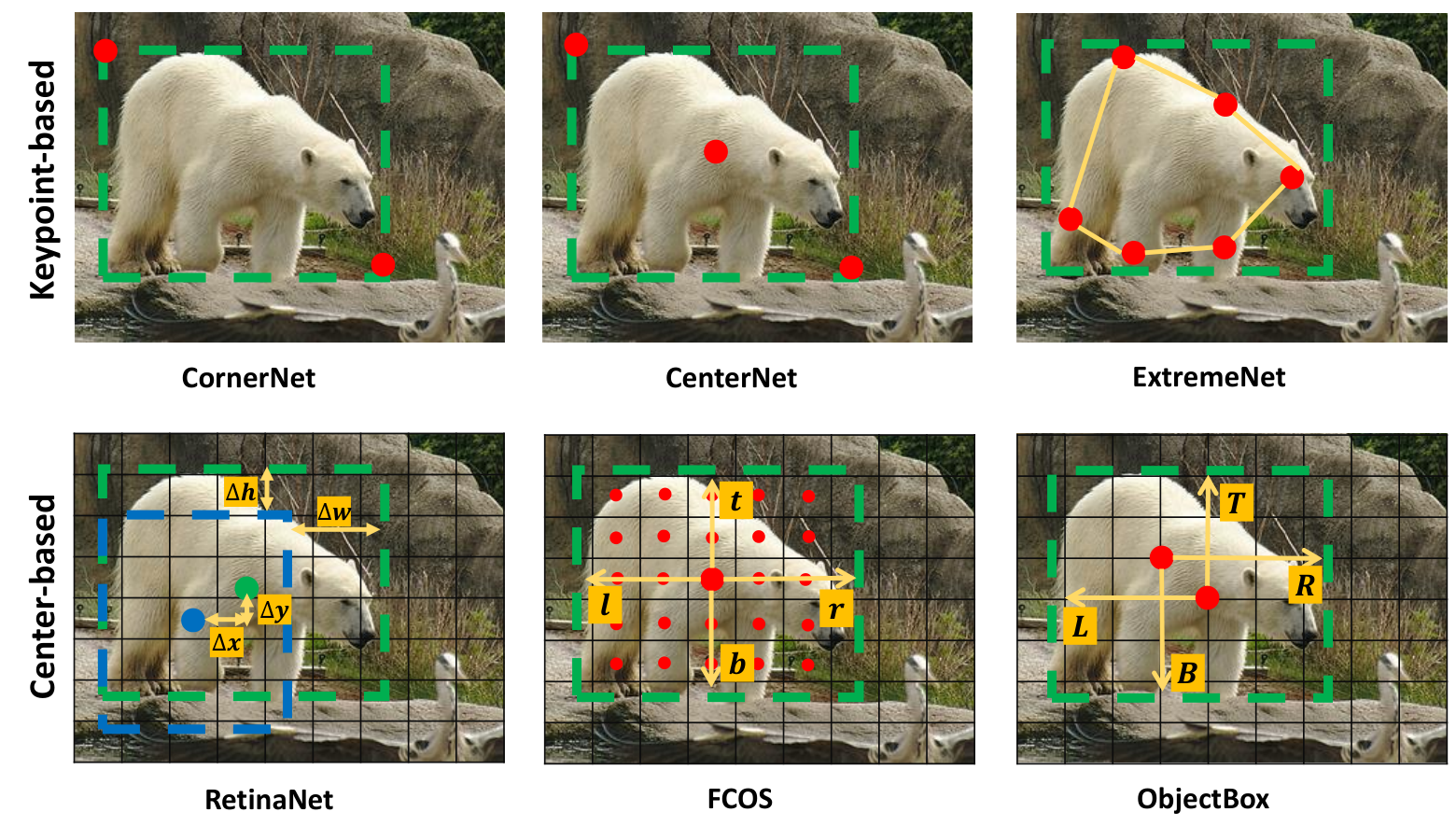
In response to these challenges, a number of anchor-free object detectors [22], [29], [16], [41], [40], [11], [35] have been recently developed, which can be categorized into keypoint-based [22], [16], [41], [40] and center-based methods [11], [29], [35]. In keypoint-based methods, multiple object points, such as center and corner points, are located using a standard keypoint estimation network (e.g., HourglassNet [21]), and grouped to bound the spatial extent of objects. They however require a complicated combinatorial grouping algorithm after keypoint detection. In contrast, center-based methods are more similar to anchor-based approaches as they use the object region of interest or central locations to define positive samples. While anchor-based methods use anchor boxes as predefined reference boxes on these central locations, anchor-free methods instead directly regress the bounding boxes at these locations (see Figure 1).

It is shown in [37] that the main difference between anchor-based and anchor-free methods in center-based approaches is the definition of positive and negative training samples, which leads to a performance gap. To distinguish between positive and negative samples, anchor-based methods use IoU to select positives in spatial and scale dimension simultaneously, whereas anchor-free methods use some spatial and scale constraints to first find candidate positives in the spatial dimension, then select final positives in the scale dimension. Nevertheless, both static strategies impose constraint thresholds to determine the boundaries between positive and negative samples, ignoring the fact that for objects with different sizes, shapes or occlusion conditions, the optimal boundaries may vary [6]. Many dynamic assignment mechanisms have been developed in response to this issue [37], [6], [13]. For instance, in [37], the division boundary is proposed to be set for each target based on some statistical criterions.
In this paper, we propose to relax all constraints imposed by static or dynamic assignment strategies and, thus, treat all objects in all scales equally. To learn the classification labels and regression offsets regardless of the object shape or size, we only regress from object central locations which are treated as shape- and size- agnostic anchors [40]. To support this, we define new regression targets as the distances from two corners of the grid cell that contains the object center, to the bounding box boundaries (, , , and in Figure 1). As illustrated in Figure 2, we use no criteria compared to other methods in different scale levels. We therefore expand the positive samples without any bells and whistles. To learn these positive samples from all scales, we propose a new scale-invariant criteria as an IoU measure which penalizes the error between target and predicted object boxes with different sizes at different scale levels.
In summary, our contribution is the proposal of a novel anchor-free object detector, ObjectBox, which is better equipped to handle the label assignment issue, and performs favorably in comparison to the state-of-the-art. Moreover, our method is plug-and-play and can be easily applied across various datasets without the need for any hyperparameter tuning. Our method is therefore more robust and generalizable, and achieves state-of-the-art results. Lastly, we will make our code implementation publicly available upon publication of this paper.
2 Related Work
2.1 Anchor-based object detectors
To localize objects at different scales with various aspect ratios, Faster R-CNN introduced anchor boxes as fixed sized bounding box proposals. The rationale behind anchor boxes is to use a set of predefined shapes (i.e. sizes and aspect ratios) as bounding box proposals, an idea which has become common in other object detection methods [24], [1], [18], [20].
Early anchor-based methods include two stages for region proposal generation and object detection, which make them unsuitable for real-time applications. To achieve real-time performance, single-shot detectors [18], [20], [24], [34] used anchors without relying on RPNs. They directly predicted bounding boxes and class probabilities from the entire image in a single evaluation. The most representative single-shot detectors are SSD [20], RetinaNet [18], and YOLO [24], [1]. Several other techniques used different variations of anchor boxes. For example, a multiple anchor learning approach was proposed in [12] to construct anchor bags and select the most representative anchors from each bag.
2.2 Anchor-free object detectors
A limitation of anchor-based methods is that they require predefined hyperparameters to specify the sizes and aspect ratios of the anchor boxes. Specifying these hyperparameters requires heuristic tuning and several empirical tricks, and is dependent on the dataset and therefore lacks generality. Anchor-free detectors have been recently proposed to overcome the drawbacks of anchor boxes. They can be categorized as keypoint-based and center-based approaches.
Keypoint-based methods detect specific object points, such as center and corner points, and group them for bounding box prediction. Although they show improved performance over anchor-based methods, the grouping procedure is time-consuming, and they usually result in a low recall rate. Some representative examples include CornerNet [16], ExtremeNet [41], CenterNet [40], [4], and CentripetalNet [3].
Center-based methods use an object region of interest or central locations to determine positive samples, which makes them more comparable to anchor-based approaches. FCOS [29], for instance, considered all locations within the object bounding box to be candidate positives and found the final positives in each scale dimension. It computed the distances from these positive locations to the four sides of the bounding box. It however generated many low-quality predicted bounding boxes from locations far from the object center. To suppress these predictions, it used a centerness score to down-weight the scores of low-quality bounding boxes. Moreover, it utilized a 5-level FPN (Feature Pyramid Network) [17] to detect objects with different sizes at different levels of feature maps. FoveaBox [14] predicted both the locations where the object center is likely to exist, and the bounding box for each positive location. FSAF (Feature Selective Anchor-Free) [42] attached an anchor-free branch to each level of the feature pyramid in RetinaNet [18].
2.3 Label assignment
It is shown in [37] that anchor-based and anchor-free methods achieve similar results if they use the same label assignment strategy. In label assignment, each feature map point is labeled positive or negative based on the object ground-truth and the assignment strategy. Some anchor-free methods such as FCOS [29] utilize static constraints to define positives, while a proper constraint may vary based on the objects’ sizes and shapes.
Many other label assignment strategies have been recently proposed. ATSS [37] (Adaptive Training Sample Selection), for example, proposed a dynamic strategy based on statistical features of the objects. In [13], the anchor assignment is modeled as a probabilistic procedure by calculating anchor scores from a detector model and maximizing the likelihood of these scores for a probability distribution. OTA [6] (Optimal Transport Assignment) proposed to formulate label assignment as an optimal transport problem, which is a variant of linear programming in optimization theory. It characterized each ground-truth as a supplier of a particular number of labels, and defines each anchor as a demander that requires one unit label. If an anchor obtains a large enough number of positive labels from a given ground-truth, it is treated as one positive anchor for that ground-truth.
These strategies, however, do not maintain equality between different objects, and they tend to assign more positive samples for larger objects. This can be alleviated by assigning the same number of positive samples and allowing learning to occur at all scales for every object regardless of its size.
3 ObjectBox
Let a training image contain objects with ground-truth , where and respectively denote the bounding box and the object class label for the th object. Each bounding box is represented by its center , width and height . Our goal is to locate these boxes in an image and assign their class labels.

3.1 Label assignment based on object central locations
The bounding box with center in the input image can be defined using its corner points as , where and denote the respective coordinates of the top-left and bottom-right corners at scale . Our method predicts bounding boxes at 3 different scales to handle object scale variations. Hence, different sizes of objects can be detected on 3 feature maps corresponding to these scales. We specifically choose strides and map each bounding box center to certain locations on these embeddings.
We map the center to the center location (i.e., the orange cell in Figure 3 (a)) in the embedding for scale , and separately compute the distances from its top-left and bottom-right corners (red circles) each respectively from two boundaries of the bounding box. Specifically, as shown in Figure 3, we compute the distances from the bottom-right corner to the left and top boundaries ( and ), and the distances from the top-left corner to the right and bottom boundaries ( and ) as follows:
| (1) |
where represent the regression targets at scale , and and denote the respective coordinates of the top-left and the bottom-right corners of the center location. It should be noted that and , where and denote the width and height of the bounding box at scale , respectively. The predictions corresponding to these distances are as follows:
| (2) |
where stands for the logistic sigmoid function, and denote the network predictions for distance values, which we enforce by sigmoid, to be in the range of 0 and 1. Multiplying by 2 allows detected values to cover a slightly larger range. With , the output is stably initialized with around zero gradient. We differentiate between different scales by multiplying to a constant scale gain, i.e., . The overall network outputs include one prediction per location per scale, each of which comprises the above-mentioned distance values, as well as an objectness score and a class label for each bounding box.
Our formulation ensures that all the distances being regressed remain positive under different conditions. As illustrated in Figure 3 (b), the 4 distances can be computed as positive values even for a small object which is contained completely within a cell at a larger stride. More importantly, we treat all the objects as positive samples at different scales. This is in contrast to existing center-based approaches (i.e., both anchor-based and anchor-free methods). In the anchor-based methods, for instance, each center location in a certain scale is seen as the center of multiple anchor boxes, and if the IoUs of the target box and these anchor boxers are not within the threshold ranges, then it is considered as a negative sample. Similarly, anchor-free methods discard some target boxes as being negative samples based on different spatial and scale constraints. FCOS [29], for example, defines a set of maximum distance values that limit the range of object sizes that can be detected at each feature level. As another example, FoveaBox [14] controls the scale range for each pyramid level by an empirically-learned parameter, while in [42], a set of constant scale factors is used to define positive and negative boxes. As seen in Figure 2, ObjectBox however treats all target boxes at all scales as positive samples. It therefore learns from all scales regardless of the object size to achieve more reliable regressions from multiple levels. As ObjectBox considers only central locations for each object, the number of positive samples per object is independent of object size.
As the geometric center of the box might lie near a boundary of the center cell, we augment the center with its neighboring cells. For example, the above location is used in addition to the center cell when the center of the bounding box is on the upper half of the cell.
Our method detects the objects from their central regions. If two boxes overlap, their centers are less likely to overlap given that it is quite rare for two box centers to be situated at the same location. In MS-COCO [19] and PASCAL VOC 2012 [5], we found no cases where centers of overlapping objects overlap. Our augmented center locations, however, can be useful in dealing with these boxes. In our experiments (Section 4.2), we show that adding more points in addition to the central locations hurts the detection performance.
Our strategy implicitly harnesses the intuition behind anchor boxes, which are usually created by clustering the dimensions of the ground truth boxes in the dataset [23]. Their dimensions are obtained as estimates of the most common shapes in different sizes. For instance, Faster R-CNN [25] and YOLO [24, 1] use three scales and three aspect ratios, yielding 9 anchors at each position. Our method however uses the central locations of the bounding boxes at each scale to generate multiple predictions for each object. Our method is also more effective than other anchor-free methods such as FCOS [29] which leverage additional levels of FPN (i.e., a total of 5 layers) to handle the overlapping bounding boxes.

3.2 Box Regression
As are distances, they can be treated independently and Mean Square Error (MSE) can be used to perform regression on these values individually. Nevertheless, such a strategy would disregard the integrity of the object bounding box. IoU (Intersection over Union or Jaccard index) loss has already been proposed to take the coverage of the predicted and ground-truth bounding box areas into consideration. IoU is a widely-used similarity metric between two shapes, which due to its appealing feature of being differentiable, can be directly used as an objective function for optimization [35, 26, 39, 31]. In object detection, IoU can encode the width, height, and location of each bounding box into a normalized measure. The IoU loss () thus allows a bounding box to be recognized as a single entity, and jointly regresses the four coordinate points of the bounding box.
IoU loss has been recently improved upon by considering different cases. For example, GIoU (Generalized IoU) loss [26] included the shape and orientation of the object in addition to the coverage area. It can find the smallest area that can simultaneously cover the predicted and ground-truth bounding boxes, and use it as the denominator to replace the original denominator used in IoU loss. DIoU (Distance IoU) loss [39] additionally emphasized the distance between the centers of the predicted and ground-truth boxes. CIoU (Complete IoU) loss [39] simultaneously included the overlapping area, the distance between center points, and the aspect ratio.
In our case, we are interested in minimizing the distance between two boxes which are each given by four distance values. As we learn from different scales for objects with different sizes (i.e., we do not differentiate between scale levels), our bounding box regression loss function should be scale-invariant. Nevertheless, -based losses grow as the scales of the bounding boxes become larger [27]. As opposed to the original IoU loss and its variants, our loss does not require the bounding box locations to be matched, since the localization task is already embedded in the process. Moreover, the predicted and ground-truth boxes share at least one point in the worst case (i.e., overlap ). This is because for each box. In this work, we propose an IoU-based loss tailored for our object detection method, which can be used to improve other anchor-free detectors as well (the experiments are provided in the supplementary materials). Our proposed loss, called SDIoU which stands for scale-invariant distance-based IoU, is directly applied on the network outputs which are distance values from the object center to top-left and bottom-right corners. Other IoU-based losses, however, work on the object center and object width and height. As SDIoU is based on the Euclidean distances between corresponding offsets of the predicted and ground-truth boxes, it can keep the box integrity and score the overlapping area in all 4 directions.
Similar to CIoU [39] and scale balanced loss [27], we consider non-overlapping areas, overlapping or intersection area, and smallest box that covers both boxes. We first compute the non-overlapping area, , by summing the squares of all the Euclidean distances between corresponding distance values as:
| (3) |
where and are the predicted and ground-truth distances, respectively. (We omit here the scale , for better readability.) Intuitively, computing the squared Euclidean distances between different distance values can effectively consider the predicted and ground-truth distances at 4 directions.
We obtain the intersection area, , by computing the square of the length of the intersection area’s diagonal as:
| (4) |
where and are the width and height of the intersection area, respectively, and are computed as:
| (5) | ||||
The smallest area that covers both predicted and ground-truth boxes, , is calculated by the square of its length as:
| (6) |
where and respectively denote ’s width and height, which are computed as:
| (7) | ||||
By minimizing , the predicted box can move towards the ground-truth box at 4 directions. We finally compute the SDIoU as:
| (8) |
where denotes a positive trade-off value that favors the overlap area (we however set in all the experiments). We use both and in the numerator to score the intersection area as well as penalizing the non-overlapping area. The predicted 4 distance values are thus enforced to faster match the ground-truth distances. The SDIoU loss is eventually defined as . Figure 4 illustrates the areas considered in our SDIoU loss.
4 Experiments
Datasets. Two common challenging datasets, MS-COCO [19] and PASCAL VOC 2012 [5], which are widely-used benchmarks for natural scene object detection, were selected to evaluate the proposed ObjectBox method and compare it against current state-of-the-art methods. MS-COCO is a challenging dataset that includes a large number of objects labeled in 80 object categories. We used the trainval35k split containing 115k images for training our network, and reported the results on the test-dev split with 20k images. The PASCAL VOC 2012 dataset consists of complex scene images of 20 diverse object classes. We trained our model using the VOC 2012 and VOC 2007 trainval splits (17k images) and tested it on the VOC 2012 test split (16k images). Experimental results on the PASCAL VOC 2012 [5] can be found in the supplementary materials (Sec. S.2).
Implementation Details. We implemented our method on two different backbones, i.e., ResNet-101 and CSPDarknet [33], [10], [1]. We use ResNet-101 which is a widely-used backbone in many object detectors to provide a fair comparison with other state-of-the-art methods. We also utilized CSPDarknet and add SPP (Spatial Pyramid Pooling) [9], [24], [1] over the backbone to increase the receptive field of the extracted features. CSPDarknet has the potential to enhance the learning abilities of the CNNs and reduce the memory cost [1].
The training hyperparameters were set to an initial learning rate of 0.01, momentum of 0.937, weight decay of 0.0005, warm-up epochs of 3, and warm-up momentum of 0.8. The initial learning rate was multiplied with a factor 0.1 at 400,000 steps, and then again at 450,000 steps. We set the batch size to 24 and used SGD optimization. We trained our models to a maximum of 300 epochs with early stopping patience of 30 epochs. The experiments were executed on a single Titan RTX GPU. The NMS (Non-Maximum Suppression) threshold was also set as in all experiments.
We used CutMix and Mosaic data augmentation during training [1]. They both mix different contexts to facilitate detection of objects outside their normal context. CutMix mixes 2 input images, while Mosaic mixes 4 training images. For each scale level , we use a multitask loss as:
| (9) |
where , , and respectively denote the classification loss, a binary cross entropy loss, and the regression loss for box offsets at scale . We use the binary cross entropy between the target classes and the predicted probabilities as our classification loss and the binary confidence score. We employ SDIoU loss as the regression loss between the proposed targets and the predicted ones. The losses are computed for each scale and are summed as .
| Avg. Precision, IoU | Avg. Precision, Area | Avg. Recall, # Dets | Avg. Recall, Area | ||||||||||
|---|---|---|---|---|---|---|---|---|---|---|---|---|---|
| Method | Backbone | AP | |||||||||||
| SSD513 [20] | ResNet-101 | 31.2 | 50.4 | 33.3 | 10.2 | 34.5 | 49.8 | 28.3 | 42.1 | 44.4 | 17.6 | 49.2 | 65.8 |
| DeNet [30] | ResNet-101 | 33.8 | 53.4 | 36.1 | 12.3 | 36.1 | 50.8 | 29.6 | 42.6 | 43.5 | 19.2 | 46.9 | 64.3 |
| F-RCNN w/ FPN [17] | ResNet-101 | 36.2 | 59.1 | 39.0 | 18.2 | 39.0 | 48.2 | - | - | - | - | - | - |
| YOLOv2 [23] | DarkNet-19 | 21.6 | 44.0 | 19.2 | 5.0 | 22.4 | 35.5 | 20.7 | 31.6 | 33.3 | 9.8 | 36.5 | 54.4 |
| RetinaNet [18] | ResNet-101 | 39.1 | 59.1 | 42.3 | 21.8 | 42.7 | 50.2 | - | - | - | - | - | - |
| YOLOv3 [24] | DarkNet-53 | 33.0 | 57.9 | 34.4 | 18.3 | 35.4 | 41.9 | - | - | - | - | - | - |
| CornerNet [16] | Hourglass-104 | 40.6 | 56.4 | 43.2 | 19.1 | 42.8 | 54.3 | 35.3 | 54.7 | 59.4 | 37.4 | 62.4 | 77.2 |
| CenterNet [4] | Hourglass-52 | 41.6 | 59.4 | 44.2 | 22.5 | 43.1 | 54.1 | 34.8 | 55.7 | 60.1 | 38.6 | 63.3 | 76.9 |
| ExtremeNet [41] | Hourglass-104 | 40.2 | 55.5 | 43.2 | 20.4 | 43.2 | 53.1 | - | - | - | - | - | - |
| FCOS [29] | ResNeXt-101 | 42.1 | 62.1 | 45.2 | 25.6 | 44.9 | 52.0 | - | - | - | - | - | - |
| ASSD513 [34] | ResNet101 | 34.5 | 55.5 | 36.6 | 15.4 | 39.2 | 51.0 | 29.9 | 45.6 | 47.6 | 22.8 | 52.2 | 67.9 |
| SaccadeNet [15] | DLA-34-DCN | 40.4 | 57.6 | 43.5 | 20.4 | 43.8 | 52.8 | - | - | - | - | - | - |
| YOLOv4 [1] | CSPDarknet | 43.5 | 65.7 | 47.3 | 26.7 | 46.7 | 53.3 | - | - | - | - | - | - |
| FoveaBox [14] | ResNeXt-101 | 43.9 | 63.5 | 47.7 | 26.8 | 46.9 | 55.6 | - | - | - | - | - | - |
| RetinaNet+CBAF [28] | ResNet-101 | 43.0 | 63.2 | 46.3 | 25.9 | 45.6 | 51.4 | - | - | - | - | - | - |
| ATSS [37] | ResNet-101 | 43.6 | 62.1 | 47.4 | 26.1 | 47.0 | 53.6 | - | - | - | - | - | - |
| PAA [13] | ResNet-101 | 44.8 | 63.3 | 48.7 | 26.5 | 48.8 | 56.3 | - | - | - | - | - | - |
| OTA [6] | ResNet-101 | 45.3 | 63.5 | 49.3 | 26.9 | 48.8 | 56.1 | - | - | - | - | - | - |
| VarifocalNet [36] | ResNet-101 | 46.0 | 64.2 | 50.0 | 27.5 | 49.4 | 56.9 | - | - | - | - | - | - |
| ObjectBox | ResNet-101 | 46.1 | 65.0 | 48.3 | 26.0 | 48.7 | 57.3 | 35.3 | 57.1 | 60.5 | 39.2 | 65.0 | 76.9 |
| ObjectBox | CSPDarknet | 46.8 | 65.9 | 49.5 | 26.8 | 49.5 | 57.6 | 36.0 | 57.5 | 60.7 | 39.4 | 65.2 | 77.0 |
4.1 MS-COCO Object Detection
Table 1 shows the evaluation results on the MS-COCO dataset. Compared to the baseline methods, ObjectBox is considerably more accurate, achieving the best AP performance of with a CSPDarknet backbone. Our method also achieves the second-best performance of with a ResNet-101 backbone. The relative improvement of (which is averaged over 10 IoU thresholds of to ) indicates that ObjectBox generates more accurate boxes with better localization. With the CSPDarknet backbone, the improvements are also achieved over 8 other metrics including , , , , , , , and . Notably, ObjectBox with ResNet-101 obtains the second-best performance over 7 different metrics. These improvements over both anchor-based and anchor-free methods are mainly due to our strategy to learn object features in different scales fairly. Nonetheless, this is not possible without regressing from the object central locations, which can be seen as shape- and size-agnostic anchors.
The relative improvement in indicates that our method can detect more small objects (which are more likely to overlap and generally harder to detect). The performance boost is also evident for when detection of larger objects can benefit from all feature maps at 3 scale levels. This is another major difference with other detectors which learn from all points in the objects. To maintain the relative equality between different objects, they consider the larger objects as positive samples only for embeddings with larger strides.
The second best performing method, VarifocalNet [36], replaces the classification score of the ground-truth class with a new IoU-aware classification score. It is built on an ATSS [37] version of FCOS [29]. In ATSS, the Adaptive Training Sample Selection (ATSS) mechanism is used to define positive and negative points on the feature pyramids during training. FoveaBox [14], which is also an anchor-free detector and concentrates on the object center, achieves . It however separates samples as positives and negatives at each scale. Improvements over FCOS [29] () shows that central regions of the objects include enough recognizable visual patterns to detect the objects if we consider positive samples from all scales, and therefore, learning all the pixels inside the bounding box is not required for a general object detection method.
It is also interesting to note that ObjectBox does not use any data-dependent hyperparameters. Other anchor-free methods which tend to address the generalization issue often use a number of such hyperparameters. FCOS [29], for example, defines a hyperparameter for thresholding the object sizes at different scales, while FoveaBox [14] defines a hyperparameter to control the scale range.
| Avg. Precision, IoU | Avg. Precision, Area | |||||||
|---|---|---|---|---|---|---|---|---|
| Experiment | Method | AP | ||||||
| A | Regression locations | (1) center | 33.1 | 56.8 | 36.0 | 17.5 | 35.2 | 42.1 |
| (2) aug. center (ObjectBox) | 46.8 | 65.9 | 49.5 | 26.8 | 49.5 | 57.6 | ||
| (3) h-centers | 42.3 | 56.9 | 46.5 | 24.1 | 45.3 | 54.2 | ||
| (4) aug. center + h-centers | 41.7 | 58.2 | 45.2 | 23.6 | 43.3 | 54.5 | ||
| (5) 4 corners | 28.2 | 51.5 | 35.6 | 16.0 | 33.9 | 41.3 | ||
| (6) 4 corners + center | 37.4 | 57.8 | 43.0 | 20.4 | 39.7 | 45.5 | ||
| B | #Pred. | 1 prediction (ObjectBox) | 46.8 | 65.9 | 49.5 | 26.8 | 49.5 | 57.6 |
| 4 predictions | 37.3 | 58.3 | 41.9 | 19.5 | 41.6 | 48.0 | ||
| C | Scale constraints | 29.6 | 45.8 | 30.4 | 17.0 | 31.8 | 40.6 | |
| 35.8 | 58.0 | 36.8 | 19.2 | 39.1 | 46.5 | |||
| 30.4 | 49.2 | 32.0 | 16.8 | 33.5 | 43.5 | |||
| 27.3 | 43.5 | 29.6 | 14.7 | 30.4 | 38.1 | |||
4.2 Ablation Study
To verify the effectiveness of our method, we performed several experiments with different settings on the MS-COCO dataset. We utilized ObjectBox with a CSPDarknet backbone in all ablation experiments.
Box regression locations. Table 2 part A shows the impact of regression from different locations by choosing the boxes to be regressed from different locations. We defined 6 cases: (1) only one location at the center (referred to as ‘center’), (2) center location augmented with its neighboring locations (as done in ObjectBox, denoted by ‘aug. center’), (3) the centers of the connecting lines between the box center and two top-left and bottom-right box corner points (referred to as ‘h-centers’), (4) central locations in (2) plus all locations in (3) (denoted by ‘aug. center + h-centers’), (5) four corners of the bounding box, and (6) corner points in (5) plus the center location. The results show that using only the center cell is not sufficient for box regression. Another important point is that (3) outperforms (1), meaning that selection of two other points close to the center is better than only center point. Removing these two locations and considering only central locations in (2) even brings further improvements. Interestingly, in (4), no improvement is seen over (3). This indicates not only that considering locations other than the central locations does not add valuable information, but also that doing so can actually degrade detection performance. The worst case occurs when we use only the corner points of the bounding box. While the performance is improved by the addition of one center location to the points in (5), the results are still far from those in (2), (3), and (4), where box regression is obtained only from points that are closer to the center locations.
Number of predicted boxes. We analyzed the influence of the number of predictions per location, and reported the results in Table 2 part B. In this experiment, we assigned 4 predictions to each location based on the offset of the object center in that location. Specifically, each location was divided into four equal finer locations, with one prediction given to each of them. When we predict 4 boxes at each location, surprisingly the performance degrades, confirming that our strategy of returning just one prediction per scale level is indeed beneficial.
Specialized feature maps. To show the impact of imposing constraints on the feature maps at different scales, we chose four sets of thresholds: (1) , (2) , (3) , and (4) . An object at scale is considered as a negative sample if or for . The negative boxes thus are not regressed. This is similar to both anchor-based and anchor-free detectors. Specifically, anchor-free methods like YOLO [24], [1] assign anchor boxes with different sizes to different feature levels, and anchor-free methods such as FCOS [29] directly limit the range of box regression for each level. The results in Table 2 part C show the high sensitivity of the performance to these thresholds. Moreover, this experiment verifies our choice of considering embeddings in all scale levels for all objects, as thresholding the feature maps drastically hurts the results.
Loss functions. To show the effectiveness of our SDIoU loss for box regression, we replaced it with three other common losses in three different experiments. We first used MSE (Mean Square Error) loss on all 4 distances separately. In the second and third experiments, we converted the 4 distances to and used the GIoU [26] and CIoU losses [39]. As observed in Table 3, these losses are not suitable in anchor-free detectors like ObjectBox. More importantly, the benefit of our IoU loss is evident from these experiments.
We provide more experiments in the supplemental materials (Sec. S.4) to verify the effectiveness of SDIoU in other anchor-free approaches like FCOS [29].
| Avg. Precision, IoU | Avg. Precision, Area | |||||
|---|---|---|---|---|---|---|
| Method | AP | |||||
| MSE | 22.6 | 44.1 | 19.4 | 12.5 | 18.3 | 35.7 |
| Adopted GIoU | 27.4 | 46.9 | 28.2 | 23.8 | 30.2 | 41.8 |
| Adopted CIoU | 27.1 | 46.5 | 28.1 | 24.0 | 30.5 | 41.0 |
| SDIoU | 46.8 | 65.9 | 49.5 | 26.8 | 49.5 | 57.6 |
5 Conclusion
ObjectBox, an anchor-free object detector, is presented without the need for any hyperparameter tuning. It uses object central locations and employs a new regression target for bounding box regression. Moreover, by relaxing the label assignment constraints, it treats all objects equally in all feature levels. A tailored IoU loss also minimizes the distance between the new regression targets and the predicted ones. It was demonstrated that using existing backbone architectures such as CSPDarknet and ResNet-101, ObjectBox compares favorably to other anchor-based and anchor-free methods.
Acknowledgments. Thanks to Geotab Inc., the City of Kingston, and the Natural Sciences and Engineering Research Council of Canada (NSERC) for their support of this work.
References
- [1] Bochkovskiy, A., Wang, C.Y., Liao, H.Y.M.: Yolov4: Optimal speed and accuracy of object detection. arXiv preprint arXiv:2004.10934 (2020)
- [2] Cai, Z., Vasconcelos, N.: Cascade r-cnn: Delving into high quality object detection. In: Proceedings of the IEEE conference on computer vision and pattern recognition. pp. 6154–6162 (2018)
- [3] Dong, Z., Li, G., Liao, Y., Wang, F., Ren, P., Qian, C.: Centripetalnet: Pursuing high-quality keypoint pairs for object detection. In: Proceedings of the IEEE/CVF conference on computer vision and pattern recognition. pp. 10519–10528 (2020)
- [4] Duan, K., Bai, S., Xie, L., Qi, H., Huang, Q., Tian, Q.: Centernet: Keypoint triplets for object detection. In: Proceedings of the IEEE International Conference on Computer Vision. pp. 6569–6578 (2019)
- [5] Everingham, M., Eslami, S.A., Van Gool, L., Williams, C.K., Winn, J., Zisserman, A.: The pascal visual object classes challenge: A retrospective. International journal of computer vision 111(1), 98–136 (2015)
- [6] Ge, Z., Liu, S., Li, Z., Yoshie, O., Sun, J.: Ota: Optimal transport assignment for object detection. In: Proceedings of the IEEE/CVF Conference on Computer Vision and Pattern Recognition. pp. 303–312 (2021)
- [7] Girshick, R.: Fast r-cnn. In: Proceedings of the IEEE international conference on computer vision. pp. 1440–1448 (2015)
- [8] He, K., Gkioxari, G., Dollár, P., Girshick, R.: Mask r-cnn. In: Proceedings of the IEEE international conference on computer vision. pp. 2961–2969 (2017)
- [9] He, K., Zhang, X., Ren, S., Sun, J.: Spatial pyramid pooling in deep convolutional networks for visual recognition. IEEE transactions on pattern analysis and machine intelligence 37(9), 1904–1916 (2015)
- [10] Huang, G., Liu, Z., Van Der Maaten, L., Weinberger, K.Q.: Densely connected convolutional networks. In: Proceedings of the IEEE conference on computer vision and pattern recognition. pp. 4700–4708 (2017)
- [11] Huang, L., Yang, Y., Deng, Y., Yu, Y.: Densebox: Unifying landmark localization with end to end object detection. arXiv preprint arXiv:1509.04874 (2015)
- [12] Ke, W., Zhang, T., Huang, Z., Ye, Q., Liu, J., Huang, D.: Multiple anchor learning for visual object detection. In: Proceedings of the IEEE/CVF Conference on Computer Vision and Pattern Recognition. pp. 10206–10215 (2020)
- [13] Kim, K., Lee, H.S.: Probabilistic anchor assignment with iou prediction for object detection. In: European Conference on Computer Vision. pp. 355–371. Springer (2020)
- [14] Kong, T., Sun, F., Liu, H., Jiang, Y., Li, L., Shi, J.: Foveabox: Beyound anchor-based object detection. IEEE Transactions on Image Processing 29, 7389–7398 (2020)
- [15] Lan, S., Ren, Z., Wu, Y., Davis, L.S., Hua, G.: Saccadenet: A fast and accurate object detector. In: Proceedings of the IEEE/CVF Conference on Computer Vision and Pattern Recognition. pp. 10397–10406 (2020)
- [16] Law, H., Deng, J.: Cornernet: Detecting objects as paired keypoints. In: Proceedings of the European Conference on Computer Vision (ECCV). pp. 734–750 (2018)
- [17] Lin, T.Y., Dollár, P., Girshick, R., He, K., Hariharan, B., Belongie, S.: Feature pyramid networks for object detection. In: Proceedings of the IEEE conference on computer vision and pattern recognition. pp. 2117–2125 (2017)
- [18] Lin, T.Y., Goyal, P., Girshick, R., He, K., Dollár, P.: Focal loss for dense object detection. In: Proceedings of the IEEE international conference on computer vision. pp. 2980–2988 (2017)
- [19] Lin, T.Y., Maire, M., Belongie, S., Hays, J., Perona, P., Ramanan, D., Dollár, P., Zitnick, C.L.: Microsoft coco: Common objects in context. In: European conference on computer vision. pp. 740–755. Springer (2014)
- [20] Liu, W., Anguelov, D., Erhan, D., Szegedy, C., Reed, S., Fu, C.Y., Berg, A.C.: Ssd: Single shot multibox detector. In: European conference on computer vision. pp. 21–37. Springer (2016)
- [21] Newell, A., Yang, K., Deng, J.: Stacked hourglass networks for human pose estimation. In: European conference on computer vision. pp. 483–499. Springer (2016)
- [22] Redmon, J., Divvala, S., Girshick, R., Farhadi, A.: You only look once: Unified, real-time object detection. In: Proceedings of the IEEE conference on computer vision and pattern recognition. pp. 779–788 (2016)
- [23] Redmon, J., Farhadi, A.: Yolo9000: better, faster, stronger. In: Proceedings of the IEEE conference on computer vision and pattern recognition. pp. 7263–7271 (2017)
- [24] Redmon, J., Farhadi, A.: Yolov3: An incremental improvement. arXiv preprint arXiv:1804.02767 (2018)
- [25] Ren, S., He, K., Girshick, R., Sun, J.: Faster r-cnn: Towards real-time object detection with region proposal networks. In: Advances in neural information processing systems. pp. 91–99 (2015)
- [26] Rezatofighi, H., Tsoi, N., Gwak, J., Sadeghian, A., Reid, I., Savarese, S.: Generalized intersection over union: A metric and a loss for bounding box regression. In: Proceedings of the IEEE Conference on Computer Vision and Pattern Recognition. pp. 658–666 (2019)
- [27] Sun, D., Yang, Y., Li, M., Yang, J., Meng, B., Bai, R., Li, L., Ren, J.: A scale balanced loss for bounding box regression. IEEE Access 8, 108438–108448 (2020)
- [28] Tang, Z., Yang, J., Pei, Z., Song, X.: Coordinate-based anchor-free module for object detection. Applied Intelligence pp. 1–15 (2021)
- [29] Tian, Z., Shen, C., Chen, H., He, T.: Fcos: Fully convolutional one-stage object detection. In: Proceedings of the IEEE International Conference on Computer Vision. pp. 9627–9636 (2019)
- [30] Tychsen-Smith, L., Petersson, L.: Denet: Scalable real-time object detection with directed sparse sampling. In: Proceedings of the IEEE international conference on computer vision. pp. 428–436 (2017)
- [31] Tychsen-Smith, L., Petersson, L.: Improving object localization with fitness nms and bounded iou loss. In: Proceedings of the IEEE conference on computer vision and pattern recognition. pp. 6877–6885 (2018)
- [32] Uzkent, B., Yeh, C., Ermon, S.: Efficient object detection in large images using deep reinforcement learning. In: The IEEE Winter Conference on Applications of Computer Vision. pp. 1824–1833 (2020)
- [33] Wang, C.Y., Mark Liao, H.Y., Wu, Y.H., Chen, P.Y., Hsieh, J.W., Yeh, I.H.: Cspnet: A new backbone that can enhance learning capability of cnn. In: Proceedings of the IEEE/CVF Conference on Computer Vision and Pattern Recognition Workshops. pp. 390–391 (2020)
- [34] Yi, J., Wu, P., Metaxas, D.N.: Assd: Attentive single shot multibox detector. Computer Vision and Image Understanding 189, 102827 (2019)
- [35] Yu, J., Jiang, Y., Wang, Z., Cao, Z., Huang, T.: Unitbox: An advanced object detection network. In: Proceedings of the 24th ACM international conference on Multimedia. pp. 516–520 (2016)
- [36] Zhang, H., Wang, Y., Dayoub, F., Sunderhauf, N.: Varifocalnet: An iou-aware dense object detector. In: Proceedings of the IEEE/CVF Conference on Computer Vision and Pattern Recognition. pp. 8514–8523 (2021)
- [37] Zhang, S., Chi, C., Yao, Y., Lei, Z., Li, S.Z.: Bridging the gap between anchor-based and anchor-free detection via adaptive training sample selection. In: Proceedings of the IEEE/CVF conference on computer vision and pattern recognition. pp. 9759–9768 (2020)
- [38] Zhang, X., Wan, F., Liu, C., Ji, R., Ye, Q.: Freeanchor: Learning to match anchors for visual object detection. Advances in neural information processing systems 32 (2019)
- [39] Zheng, Z., Wang, P., Liu, W., Li, J., Ye, R., Ren, D.: Distance-iou loss: Faster and better learning for bounding box regression. In: AAAI. pp. 12993–13000 (2020)
- [40] Zhou, X., Wang, D., Krähenbühl, P.: Objects as points. arXiv preprint arXiv:1904.07850 (2019)
- [41] Zhou, X., Zhuo, J., Krahenbuhl, P.: Bottom-up object detection by grouping extreme and center points. In: Proceedings of the IEEE Conference on Computer Vision and Pattern Recognition. pp. 850–859 (2019)
- [42] Zhu, C., He, Y., Savvides, M.: Feature selective anchor-free module for single-shot object detection. In: Proceedings of the IEEE/CVF Conference on Computer Vision and Pattern Recognition. pp. 840–849 (2019)