This work has been submitted to the IEEE for possible publication. Copyright may be transferred without notice, after which this version may no longer be accessible.

Strict Intuitionistic Fuzzy Distance/Similarity Measures Based on Jensen-Shannon Divergence

Xinxing Wu Zhiyi Zhu Guanrong Chen Tao Wang Peide Liu Thanks: X. Wu is with (1) the School of Sciences, Southwest Petroleum University, Chengdu, Sichuan 610500, China; (2) the Institute for Artificial Intelligence, Southwest Petroleum University, Chengdu, Sichuan 610500, China. (3) the Zhuhai College of Jilin University, Zhuhai, Guangdong 519041, China. e-mail: (wuxinxing5201314@163.com). Thanks: Z. Zhu is with the School of Sciences, Southwest Petroleum University, Chengdu, Sichuan 610500, China. e-mail: (zhuzhiyi2019@163.com). Thanks: G. Chen is with the Department of Electrical Engineering, City University of Hong Kong, Hong Kong SAR, China. e-mail: (eegchen@cityu.edu.hk). Thanks: T. Wang is with the School of Sciences, Southwest Petroleum University, Chengdu, Sichuan 610500, China. e-mail: (wt1994math@163.com). Thanks: P. Liu is with the School of Management Science and Engineering, Shandong University of Finance and Economics, Jinan, Shandong 250014, China. e-mail: (peide.liu@gmail.com). Thanks: All correspondences should be addressed to X. Wu. Thanks: This work was supported by the National Natural Science Foundation of China (Nos.˜11601449 and 71771140) and the Key Natural Science Foundation of Universities in Guangdong Province (No. 2019KZDXM027).

Abstract

Being a pair of dual concepts, the normalized distance and similarity measures are very important tools for decision-making and pattern recognition under intuitionistic fuzzy sets framework. To be more effective for decision-making and pattern recognition applications, a good normalized distance measure should ensure that its dual similarity measure satisfies the axiomatic definition. In this paper, we first construct some examples to illustrate that the dual similarity measures of two nonlinear distance measures introduced in [A distance measure for intuitionistic fuzzy sets and its application to pattern classification problems, IEEE Trans. Syst., Man, Cybern., Syst., vol. 51, no. 6, pp. 3980–3992, 2021] and [Intuitionistic fuzzy sets: spherical representation and distances, Int. J. Intell. Syst., vol. 24, no. 4, pp. 399–420, 2009] do not meet the axiomatic definition of intuitionistic fuzzy similarity measure. We show that (1) they cannot effectively distinguish some intuitionistic fuzzy values (IFVs) with obvious size relationship; (2) except for the endpoints, there exist infinitely many pairs of IFVs, where the maximum distance 1 can be achieved under these two distances; leading to counter-intuitive results. To overcome these drawbacks, we introduce the concepts of strict intuitionistic fuzzy distance measure (SIFDisM) and strict intuitionistic fuzzy similarity measure (SIFSimM), and propose an improved intuitionistic fuzzy distance measure based on Jensen-Shannon divergence. We prove that (1) it is a SIFDisM; (2) its dual similarity measure is a SIFSimM; (3) its induced entropy is an intuitionistic fuzzy entropy. Comparative analysis and numerical examples demonstrate that our proposed distance measure is completely superior to the existing ones.

Index Terms:

Distance measure, similarity measure, strict similarity measure, intuitionistic fuzzy set, Jensen-Shannon divergence.

I Introduction

To deal with the ubiquitous uncertainty and fuzziness in real life, Zadeh (1965) [1] presented the fuzzy set (FS) theory by applying membership degrees to measure the importance of a fuzzy element. Zadeh’s FS generalized the concept of crisp sets, which is described by a characteristic function that can take any value in the interval $[0,1]$ . However, duo to the limitation of a membership function that only indicates two (supporting and opposing) states of fuzziness, the fuzzy sets cannot express the neutral state of “this and also that”. As a remedy to this, Atanassov [2] generalized Zadeh’s fuzzy set by introducing the concept of intuitionistic fuzzy sets (IFSs) (see also [3]), which was characterized by a membership function and a non-membership function simultaneously, satisfying the condition that the sum of the membership degree and the non-membership degree at every point is less than or equal to $1$ . Moreover, in dealing with many practical problems, it is not appropriate for experts to precisely express their decisions with crisp numbers due to the complexity and uncertainty of available information. Based on this observation, Atanassov and Gargov [4] further extended IFSs to interval-valued intuitionistic fuzzy sets (IVIFSs) (see also [5]), replacing the membership degree and the non-membership degree by some closed intervals in $[0,1]$ .

To assess the differences of IFSs, the normalized IF distance measure (IFDisM) and the IF similarity measure (IFSimM), being a pair of dual concepts (see [6]), are important tools for decision-making ([7, 8, 9, 10]), pattern recognition ([11, 12, 13, 14, 15, 16, 17, 18]), medical diagnosis ([19, 20, 10]), clustering analysis ([21, 20]), image processing ([22, 10]), and data mining under intuitionistic fuzzy sets framework. Motivated by the similarity measure for Zadeh’s fuzzy sets, Li and Cheng [11] introduced the concept of similarity measure (SimM) for IFSs, which was improved by Mitchell [23], and applied to pattern recognition problems. Recently, Szmidt [24] presented an overview on IFDisMs and IFSimMs. The research on IFDisMs and IFSimMs focuses on two aspects, one is the two-dimensional (2-D) representation of IFSs, which only considers the membership and nonmembership degrees, and the other is the three-dimensional (3-D) representation of IFSs, which simultaneously considers the membership, nonmembership, and indeterminacy degrees. However, noticeably, because the indeterminacy degree is uniquely determined by the membership and nonmembership degrees, the space of all IFVs is essentially a 2-D topological structure. This indicates a serious problem that many existing distance and similarity measures via 3-D representation of IFSs, including Euclidean similarity measure in [24] and Minkowski similarity measure in ([7, 25]), do not meet the axiomatic definition of IFSimMs (see [26, Section 3]).

For 2-D IFDisMs and IFSimMs, Szmidt and Kacprzyk [27] presented the normalized Hamming distance and normalized Euclidean distance for IFSs. Grzegorzewski [28] proposed an IFDisM by using the Hausdorff metric for closed intervals (also see [29]). Wang and Xin [30] introduced the axiomatic definition of distance measure as a dual concept of the similarity measure for IFSs and constructed some new 2-D IFDisMs by combining the 2-D Hamming IFDisM [27] and the 2-D Hausdorff IFDisM [28]. Further, based on IFDisMs introduced by Wang and Xin [30], Xu and Chen [31] presented some new IFSimMs.

For 3-D IFDisMs and IFSimMs, Xu and Chen [31] suggested some IFSimMs based on the idea of TOPSIS of Hwang and Yoon [32]. Wu et al. [26] pointed out that the IFSimM in [31, Eq. 14] based on the normalized Euclidean distance does not satisfy the axiomatic definition of IFSimMs. Motivated by the divergence measure in information theory, Chen et al. [15] introduced a novel IFSimM using centroid points of transformed right-angled TrFNs. Yang and Chiclana [33] constructed a nonlinear spherical distance measure for IFSs by using the ‘ $\arccos$ ’ function. Hung and Yang [34] constructed a $J_{\gamma}$ -divergence ( $\gamma>0$ ) for IFSs and proved that it satisfies the axiomatic definition of IFDisM of Wang and Xin [30] for $\gamma\in[1,2]$ . Joshi and Kumar [35] obtained a dissimilarity Jensen-Shannon divergence measure for IFSs. In fact, this dissimilarity measure is equivalent to the $J_{1}$ -divergence in [34]. Recently, Xiao [18] proposed a new IFDisM $\bm{d}_{\chi}$ based on the Jensen-Shannon divergence and showed that this distance measure is superior to those in [27, 28, 30, 36, 37, 38, 39]. By direct calculation, it is easy to see that $\ln 2\cdot\bm{d}_{\chi}=\sqrt{J_{1}}$ , i.e., Xiao’s distance measure $\bm{d}_{\chi}$ is a special case of Hung and Yang’s $J_{\gamma}$ -divergence (see Section III). For more results on the IFDisMs and IFSimMs, see [24, 25, 40]. It should be noted that because the axiomatic definition (S4) of IFSimMs requires the admissibility with Atanassov’s partial order ‘ $\subset$ ’, and that Atanassov’s partial order only indicates the size relationship for membership degrees and non-membership degrees, implying that many existing 3-D IFSimMs may violate the axiomatic definition (S4) of IFSimMs.

We will provide Examples 1–3 below to show that Xiao’s distance measure [18], Hung and Yang’s $J_{1}$ -divergence [34], and Joshi and Kumar’s dissimilarity Jensen-Shannon divergence measure in [35] have the follows three drawbacks: (1) its dual similarity measure does not satisfy the axiomatic definition (S4) of Definition 2; (2) it cannot effectively distinguish some IFVs/IFSs with obvious size relationship; (3) Except for the endpoints $\langle 1,0\rangle$ and $\langle 0,1\rangle$ , there exist infinitely many pairs of IFVs, where the maximum distance $1$ can be achieved under these distances. Meanwhile, observing from Examples 4 and 10 below, Yang and Chiclana’s spherical distance measure in [33] has the same drawbacks. To distinguish IFVs more effectively and overcome the above three drawbacks for IFDisMs/IFSimMs, we introduce the concepts of strict intuitionistic fuzzy similarity measure (SIFSimM) and strict intuitionistic fuzzy distance measure (SIFDisM) and construct a novel IFDisM based on Jensen-Shannon divergence measure. We demonstrate that its dual similarity measure is a SIFSimM and its induced entropy measure meets the axiomatic definition of IF entropy. Moreover, we present some comparative analysis to illustrate that our proposed distance measure is completely superior to the existing IFDisMs; in particular, it is much better than Xiao’s distance measure in [18], Hung and Yang’s $J_{\alpha}$ -divergence in [34], Joshi and Kumar’s dissimilarity divergence in [35], and Yang and Chiclana’s spherical distance in [33]. Finally, to demonstrate the effectiveness of our proposed IFSimM, we apply it to a practical pattern recognition problem.

II Preliminaries

II-A Intuitionistic fuzzy set (IFS)

Definition 1 ([3, Definition 1.1])

Let $X$ be the universe of discourse (UOD). An intuitionistic fuzzy set (IFS) $I$ in $X$ is defined as

{\small I=\left\{\frac{\langle\mu_{{}_{I}}(x),\nu_{{}_{I}}(x)\rangle}{x}~\Big|~x\in X\right\},}

(1)

where the functions $\mu_{{}_{I}}:X\longrightarrow[0,1]$ and $\nu_{{}_{I}}:X\longrightarrow[0,1]$ define the degree of membership and the degree of non-membership of the element $x\in X$ to the set $I$ , respectively, and for every $x\in X$ , $\mu_{{}_{I}}(x)+\nu_{{}_{I}}(x)\leq 1.$

Let $\mathrm{IFS}(X)$ denote the set of all IFSs in $X$ . For $I\in\mathrm{IFS}(X)$ , the indeterminacy degree $\pi_{{}_{I}}(x)$ of an element $x$ belonging to $I$ is defined by $\pi_{{}_{I}}(x)=1-\mu_{{}_{I}}(x)-\nu_{{}_{I}}(x)$ . Clearly, each subset $A$ of $X$ can be expressed as an IFS, $A=\left\{\frac{\langle\bm{1}_{A}(x),\bm{1}_{X\backslash A}(x)\rangle}{x}\mid x\in X\right\}$ , which is also called a crisp set. In [41, 40], the pair $\langle\mu_{{}_{I}}(x),\nu_{{}_{I}}(x)\rangle$ is called an intuitionistic fuzzy value (IFV) or an intuitionistic fuzzy number (IFN). For convenience, use $\alpha=\langle\mu_{\alpha},\nu_{\alpha}\rangle$ to represent an IFV $\alpha$ , which satisfies $\mu_{\alpha}\in[0,1]$ , $\nu_{\alpha}\in[0,1]$ , and $0\leq\mu_{\alpha}+\nu_{\alpha}\leq 1$ . Let $\Theta$ denote the set of all IFVs, i.e., $\Theta=\{\langle\mu,\nu\rangle\in[0,1]^{2}\mid\mu+\nu\leq 1\}$ . For $\alpha=\langle\mu_{\alpha},\nu_{\alpha}\rangle\in\Theta$ , the complement $\alpha^{\complement}$ of $\alpha$ is $\alpha^{\complement}=\langle\nu_{\alpha},\mu_{\alpha}\rangle$ .

Atanassov’s order ‘ $\subset$ ’ [3], defined by the property that $\alpha\subset\beta$ if and only if $\alpha\cap\beta=\alpha$ , is a partial order on $\Theta$ . Clearly, $\alpha\subset\beta$ if and only if $\mu_{\alpha}\leq\mu_{\beta}$ and $\nu_{\alpha}\geq\nu_{\beta}$ . The order ‘ $\subsetneqq$ ’ on $\Theta$ is defined by the property $\alpha\subsetneqq\beta$ if and only if $\alpha\subset\beta$ and $\alpha\neq\beta$ .

II-B Similarity/Distance measures for IFSs

Definition 2 ([40, 25])

A mapping $\mathbf{S}:\Theta\times\Theta\longrightarrow[0,1]$ is called an intuitionistic fuzzy similarity measure (IFSimM) on $\Theta$ if it satisfies the following conditions: for any $\alpha_{1}$ , $\alpha_{2}$ , $\alpha_{3}\in\Theta$ ,

(S1)

$0\leq\mathbf{S}(\alpha_{1},\alpha_{2})\leq 1$ .
(S2)

$\mathbf{S}(\alpha_{1},\alpha_{2})=1$ if and only if $\alpha_{1}=\alpha_{2}$ .
(S3)

$\mathbf{S}(\alpha_{1},\alpha_{2})=\mathbf{S}(\alpha_{2},\alpha_{1})$ .
(S4)

If $\alpha_{1}\subset\alpha_{2}\subset\alpha_{3}$ , then $\mathbf{S}(\alpha_{1},\alpha_{3})\leq\mathbf{S}(\alpha_{1},\alpha_{2})$ and $\mathbf{S}(\alpha_{1},\alpha_{3})\leq\mathbf{S}(\alpha_{2},\alpha_{3})$ .

Definition 3 ([40, 25])

Let $X$ be a UOD. A mapping $\mathbf{S}:\mathrm{IFS}(X)\times\mathrm{IFS}(X)\longrightarrow[0,1]$ is called an intuitionistic fuzzy similarity measure (IFSimM) on $\mathrm{IFS}(X)$ if it satisfies the following conditions: for any $I_{1}$ , $I_{2}$ , $I_{3}\in\mathrm{IFS}(X)$ ,

(S1)

$0\leq\mathbf{S}(I_{1},I_{2})\leq 1$ .
(S2)

$\mathbf{S}(I_{1},I_{2})=1$ if and only if $I_{1}=I_{2}$ .
(S3)

$\mathbf{S}(I_{1},I_{2})=\mathbf{S}(I_{2},I_{1})$ .
(S4)

If $I_{1}\subset I_{2}\subset I_{3}$ , then $\mathbf{S}(I_{1},I_{3})\leq\mathbf{S}(I_{1},I_{2})$ and $\mathbf{S}(I_{1},I_{3})$ $\leq\mathbf{S}(I_{2},I_{3})$ .

To effectively compare and distinguish IFVs and IFSs, we introduce the concept of strict intuitionistic fuzzy similarity/distance measure as follows.

Definition 4

A mapping $\mathbf{S}:\Theta\times\Theta\longrightarrow[0,1]$ is called a strict intuitionistic fuzzy similarity measure (SIFSimM) on $\Theta$ if, for any $\alpha_{1}$ , $\alpha_{2}$ , $\alpha_{3}\in\Theta$ , it satisfies (Sl)–(S3) in Definition 2 and (S4^′) and (S5) described by

(S4^′)

(Strict distinctiveness) If $\alpha_{1}\subsetneqq\alpha_{2}\subsetneqq\alpha_{3}$ , then $\mathbf{S}(\alpha_{1},\alpha_{3})<\mathbf{S}(\alpha_{1},\alpha_{2})$ and $\mathbf{S}(\alpha_{1},\alpha_{3})<\mathbf{S}(\alpha_{2},\alpha_{3})$ .
(S5)

(Extreme dissimilarity on endpoints) $\mathbf{S}(\alpha_{1},\alpha_{2})=0$ if and only if ( $\alpha_{1}=\langle 0,1\rangle$ and $\alpha_{2}=\langle 1,0\rangle$ ) or ( $\alpha_{1}=\langle 1,0\rangle$ and $\alpha_{2}=\langle 0,1\rangle$ ).

Property (S4^′) indicates that the similarity measure $\mathbf{S}$ can strictly distinguish every pair of different IFVs under Atanassov-order ‘ $\subset$ ’. Property (S5) indicates that it is extremely unsimilar (similarity measure is zero) for a pair of IFVs depending only on two endpoints.

Definition 5

Let $X$ be a UOD. A mapping $\mathbf{S}:\mathrm{IFS}(X)\times\mathrm{IFS}(X)\longrightarrow[0,1]$ is called a strict intuitionistic fuzzy similarity measure (SIFSimM) on $\mathrm{IFS}(X)$ if, for any $I_{1}$ , $I_{2}$ , $I_{3}\in\mathrm{IFS}(X)$ , it satisfies (Sl)–(S3) in Definition 3 and (S4^′) and (S5) described by

(S4^′)

If $I_{1}\subsetneqq I_{2}\subsetneqq I_{3}$ , then $\mathbf{S}(I_{1},I_{3})<\mathbf{S}(I_{1},I_{2})$ and $\mathbf{S}(I_{1},I_{3})$ $<\mathbf{S}(I_{2},I_{3})$ .
(S5)

$\mathbf{S}(I_{1},I_{2})=0$ if and only if, for any $x\in X$ , ( $I_{1}(x)=\langle 0,1\rangle$ and $I_{2}(x)=\langle 1,0\rangle$ ) or ( $I_{1}(x)=\langle 1,0\rangle$ and $I_{2}(x)=\langle 0,1\rangle$ ).

Remark 1

Property (S5) can be equivalently expressed as that $\mathbf{S}(I_{1},I_{2})=0$ if and only if $I_{1}$ is a crisp set and $I_{1}=I_{2}^{\complement}$ .

Dually, a mapping $d:\mathrm{IFS}(X)\times\mathrm{IFS}(X)\longrightarrow[0,1]$ is called a strict intuitionistic fuzzy distance measure (SIFDisM) on $\mathrm{IFS}(X)$ if it satisfies the following conditions:

(D1)

The mapping $d$ is a distance measure on $\mathrm{IFS}(X)$ (see [24, Definition 3.1]);
(D2)

The mapping $\mathbf{S}(\alpha,\beta)=1-d(\alpha,\beta)$ is a SIFSimM on $\mathrm{IFS}(X)$ .

II-C Entropy measure for IFSs

Entropy is an important information measure. Szmidt and Kacprzyk [42] gave the axiomatic definition of entropy measure for IFSs as follows:

Definition 6 ([42])

A mapping $E:\Theta\longrightarrow[0,1]$ is called an intuitionistic fuzzy entropy measure (IFEM) on $\Theta$ if it satisfies the following conditions: for any $\alpha$ , $\beta\in\Theta$ ,

(E1)

$E(\alpha)=0$ if and only if $\alpha=\langle 1,0\rangle$ or $\alpha=\langle 0,1\rangle$ .
(E2)

$E(\alpha)=1$ if and only if $\mu_{\alpha}=\nu_{\alpha}$ .
(E3)

$E(\alpha)=E(\alpha^{\complement})$ .
(E4)

$E(\alpha)\leq E(\beta)$ whenever it holds either $\mu_{\alpha}\leq\mu_{\beta}\leq\nu_{\beta}\leq\nu_{\alpha}$ or $\mu_{\alpha}\geq\mu_{\beta}\geq\nu_{\beta}\geq\nu_{\alpha}$ .

Definition 7 ([42])

Let $X$ be a UOD. A mapping $E:\mathrm{IFS}(X)\longrightarrow[0,1]$ is called an intuitionistic fuzzy entropy measure (IFEM) on $\mathrm{IFS}(X)$ if it satisfies the following conditions: for any $I_{1}$ , $I_{2}\in\mathrm{IFS}(X)$ ,

(E1)

$E(I_{1})=0$ if and only if $I_{1}$ is a crisp set.
(E2)

$E(I_{1})=1$ if and only if, for any $x\in X$ , $\mu_{I_{1}}(x)=\nu_{I_{1}}(x)$ .
(E3)

$E(I_{1})=E(I_{1}^{\complement})$ .
(E4)

$E(I_{1})\leq E(I_{2})$ if, for any $x\in X$ , it holds either $\mu_{I_{1}}(x)\leq\mu_{I_{2}}(x)\leq\nu_{I_{2}}(x)\leq\nu_{I_{1}}(x)$ or $\mu_{I_{1}}(x)\geq\mu_{I_{2}}(x)\geq\nu_{I_{2}}(x)\geq\nu_{I_{1}}(x)$ .

III The drawbacks of Xiao’s distance measure $d_{\widetilde{\chi}}$

Let $X=\{x_{1},x_{2},\ldots,x_{n}\}$ be a finite UOD and $I_{1}=\Big\{\frac{\alpha_{j}^{(1)}}{x_{j}}\mid 1\leq j\leq n,\alpha_{j}^{(1)}\in\Theta\Big\}$ and $I_{2}=\Big\{\frac{\alpha_{j}^{(2)}}{x_{j}}\mid 1\leq j\leq n,\alpha_{j}^{(2)}\in\Theta\Big\}$ be two IFSs on $X$ . Based on Jensen-Shannon divergence, Xiao [18] introduced a new distance measure $\bm{d}_{\widetilde{\chi}}$ for IFSs as follows:

\begin{split}&\bm{d}_{\widetilde{\chi}}(I_{1},I_{2})\\ =&\frac{1}{n}\sum_{j=1}^{n}\left[\frac{1}{2}\left(\mu_{I_{1}}(x_{j})\cdot\log_{2}\frac{2\mu_{I_{1}}(x_{j})}{\mu_{I_{1}}(x_{j})+\mu_{I_{2}}(x_{j})}\right.\right.\\ &\quad\quad\quad+\mu_{I_{2}}(x_{j})\cdot\log_{2}\frac{2\mu_{I_{2}}(x_{j})}{\mu_{I_{1}}(x_{j})+\mu_{I_{2}}(x_{j})}\\ &\quad\quad\quad+\nu_{I_{1}}(x_{j})\cdot\log_{2}\frac{2\nu_{I_{1}}(x_{j})}{\nu_{I_{1}}(x_{j})+\nu_{I_{2}}(x_{j})}\\ &\quad\quad\quad+\nu_{I_{2}}(x_{j})\cdot\log_{2}\frac{2\nu_{I_{2}}(x_{j})}{\nu_{I_{1}}(x_{j})+\nu_{I_{2}}(x_{j})}\\ &\quad\quad\quad+\pi_{I_{1}}(x_{j})\cdot\log_{2}\frac{2\pi_{I_{1}}(x_{j})}{\pi_{I_{1}}(x_{j})+\pi_{I_{2}}(x_{j})}\\ &\quad\quad\quad\left.\left.+\pi_{I_{2}}(x_{j})\cdot\log_{2}\frac{2\pi_{I_{2}}(x_{j})}{\pi_{I_{1}}(x_{j})+\pi_{I_{2}}(x_{j})}\right)\right]^{0.5},\end{split}

(2)

where $\alpha_{j}^{(1)}=\langle\mu_{I_{1}}(x_{i}),\nu_{I_{1}}(x_{j})\rangle$ and $\alpha_{j}^{(2)}=\langle\mu_{I_{2}}(x_{i}),$ $\nu_{I_{2}}(x_{j})\rangle$ . Its dual similarity measure $\mathbf{S}_{\widetilde{\chi}}$ is defined by $\mathbf{S}_{\widetilde{\chi}}(I_{1},I_{2})=1-\bm{d}_{\widetilde{\chi}}(I_{1},I_{2})$ .

The following examples show that Xiao’s distance measure defined by Eq. (2) has some drawbacks: (1) its dual similarity measure $\mathbf{S}_{\widetilde{\chi}}$ does not satisfy the axiomatic definition (S4) of Definition 2; (2) it cannot effectively distinguish some IFVs/IFSs with obvious size relationship; (3) Except for the endpoints $\langle 1,0\rangle$ and $\langle 0,1\rangle$ , there exist infinitely many pairs such that the maximum distance $1$ can be achieved under this distance.

Example 1

Let the UOD $X=\{x\}$ and choose $I_{1}=\left\{\frac{\langle 0.33,0.36\rangle}{x}\right\}$ , $I_{2}=\left\{\frac{\langle\frac{1}{3},\frac{1}{3}\rangle}{x}\right\}$ , and $I_{3}=\left\{\frac{\langle 0.334,0.333333\rangle}{x}\right\}\in\mathrm{IFS}(X)$ . Clearly, $I_{1}\subset I_{2}\subset I_{3}$ . Meanwhile, by Eq. (2) and direct calculation, we have $\mathbf{S}_{\widetilde{\chi}}(I_{1},I_{2})=1-\bm{d}_{\widetilde{\chi}}(I_{1},I_{2})=0.9738972$ and $\mathbf{S}_{\widetilde{\chi}}(I_{1},I_{3})=1-\bm{d}_{\widetilde{\chi}}(I_{1},I_{3})=0.9741713$ , and thus $\mathbf{S}_{\widetilde{\chi}}(I_{1},I_{2})<\mathbf{S}_{\widetilde{\chi}}(I_{1},I_{3})$ . This contradicts the axiomatic definition (S4) of Definition 2 because $I_{1}\subset I_{2}\subset I_{3}$ .

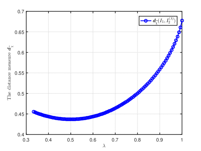
Furthermore, take $I_{2}^{(\lambda)}=\left\{\frac{\langle\frac{1}{3},\lambda\rangle}{x}\right\}$ and $I_{3}^{(\lambda)}=\left\{\frac{\langle 0.334,\lambda\rangle}{x}\right\}\in\mathrm{IFS}(X)$ in Example 1. By varying the parameter $\lambda$ from $0$ to $0.36$ , Fig. 1 visualizes the changing trend of distances between $I_{2}^{(\lambda)}$ and $I_{1}$ , and between $I_{3}^{(\lambda)}$ and $I_{1}$ , based on the distance measure $\bm{d}_{\widetilde{\chi}}$ . Observing from Fig. 1, it is clear that there exists $\lambda^{*}\in(0,0.36)$ (the intersection of the two curves in Fig. 1) such that, for any $0<\lambda<\lambda^{*}$ , it holds that $\bm{d}_{\widetilde{\chi}}(I_{1},I_{2}^{(\lambda)})>\bm{d}_{\widetilde{\chi}}(I_{1},I_{3}^{(\lambda)})$ . This further illustrates the unreasonableness of the distance measure $\bm{d}_{\widetilde{\chi}}$ since $I_{1}\subset I_{2}^{(\lambda)}\subset I_{3}^{(\lambda)}$ .

Refer to caption — Fig. 1: The distance measures $\bm{d}_{\widetilde{\chi}}(I_{1},I_{2}^{(\lambda)})$ and $\bm{d}_{\widetilde{\chi}}(I_{1},I_{3}^{(\lambda)})$ in Example 1

Hung and Yang [29] introduced the $J_{\gamma}$ -divergence to measure the difference between two IFVs as follows: for $\alpha$ , $\beta\in\Theta$ ,

•

If $\gamma\in(0,1)\cup(1,+\infty)$ , $J_{\gamma}(\alpha,\beta)=\frac{-1}{\gamma-1}\big[(\frac{\mu_{\alpha}+\mu_{\beta}}{2})^{\gamma}-\frac{1}{2}(\mu_{\alpha}^{\gamma}+\mu_{\beta}^{\gamma})+(\frac{\nu_{\alpha}+\nu_{\beta}}{2})^{\gamma}-\frac{1}{2}(\nu_{\alpha}^{\gamma}+\nu_{\beta}^{\gamma})+(\frac{\pi_{\alpha}+\pi_{\beta}}{2})^{\gamma}-\frac{1}{2}(\pi_{\alpha}^{\gamma}+\pi_{\beta}^{\gamma})\big]$ ;
•

If $\gamma=1$ , $J_{\gamma}(\alpha,\beta)=\frac{-1}{2}\big[(\mu_{\alpha}+\mu_{\beta})\ln(\frac{\mu_{\alpha}+\mu_{\beta}}{2})-\mu_{\alpha}\cdot\ln\mu_{\alpha}-\mu_{\beta}\cdot\ln\mu_{\beta}+(\nu_{\alpha}+\nu_{\beta})\ln(\frac{\nu_{\alpha}+\nu_{\beta}}{2})-\nu_{\alpha}\cdot\ln\nu_{\alpha}-\nu_{\beta}\cdot\ln\nu_{\beta}+(\pi_{\alpha}+\pi_{\beta})\ln(\frac{\pi_{\alpha}+\pi_{\beta}}{2})-\pi_{\alpha}\cdot\ln\pi_{\alpha}-\pi_{\beta}\cdot\ln\pi_{\beta}\big]$ .

Remark 2

Joshi and Kumar [35] introduced an IF dissimilarity divergence $\widehat{DJS}$ , which is equivalent to the $J_{1}$ -divergence of Hung and Yang [29]. By direct calculation, it can be verified that $\sqrt{\widehat{DJS}(\alpha,\beta)}=\sqrt{J_{1}(\alpha,\beta)}=\ln 2\cdot\bm{d}_{\chi}(\alpha,\beta)$ , and thus Example 1 also indicates that [29, Theorem 1 (D3)] and [35, Subsection 3.3] do not hold.

The following example illustrates the unreasonableness of Xiao’s distance measure $\bm{d}_{\widetilde{\chi}}$ from another perspective.

Example 2

Let the UOD $X=\{x\}$ and choose $I_{1}=\left\{\frac{\langle\frac{1}{3},\frac{1}{3}\rangle}{x}\right\}$ and $I_{2}^{(\lambda)}=\left\{\frac{\langle\lambda,0.00001\rangle}{x}\right\}\in\mathrm{IFS}(X)$ . By varying the parameter $\lambda$ from $\frac{1}{3}$ to $1$ , Fig. 2 visualizes the changing trend of distances between $I_{2}^{(\lambda)}$ and $I_{1}$ by using Xiao’s distance measure $\bm{d}_{\widetilde{\chi}}$ . Observing from Fig. 2, it is clear that, for any $\lambda_{1}$ , $\lambda_{2}\in(\frac{1}{3},0.5)$ with $\lambda_{1}<\lambda_{2}$ , it holds that $\bm{d}_{\widetilde{\chi}}(I_{1},I_{2}^{(\lambda_{1})})>\bm{d}_{\widetilde{\chi}}(I_{1},I_{2}^{(\lambda_{2})})$ , which contradicts the fact that $I_{1}\subset I_{2}^{\lambda_{1}}\subset I_{2}^{\lambda_{2}}$ . This also illustrates the unreasonableness of the distance measure $\bm{d}_{\widetilde{\chi}}$ .

Example 3

Assume that the IFSs $I_{1}$ , $I_{1}^{\prime}$ , $I_{2}$ , and $I_{3}$ on UOD $X=\{x\}$ are given by $I_{1}=\left\{\frac{\langle 1,0\rangle}{x}\right\}$ , $I_{1}^{\prime}=\left\{\frac{\langle 0,1\rangle}{x}\right\}$ , $I_{2}^{(\lambda)}=\left\{\frac{\langle\lambda,0\rangle}{x}\right\}$ , and $I_{3}^{(\lambda)}=\left\{\frac{\langle\lambda,1-\lambda\rangle}{x}\right\}$ , where $0\leq\lambda\leq 1$ . By direct calculation, it follows from Eq. (2) that

\begin{split}&\bm{d}_{\widetilde{\chi}}(I_{1},I_{2}^{(\lambda)})\\ =&\sqrt{\frac{1}{2}\left[\log_{2}\frac{2}{1+\lambda}+\lambda\log_{2}\frac{2\lambda}{1+\lambda}+(1-\lambda)\log_{2}\frac{2(1-\lambda)}{1-\lambda}\right]}\\ =&\sqrt{\frac{1}{2}\left[\log_{2}\frac{2}{1+\lambda}+\lambda\log_{2}\frac{2\lambda}{1+\lambda}+(1-\lambda)\right]}\\ =&\bm{d}_{\widetilde{\chi}}(I_{1},I_{3}^{(\lambda)}),\end{split}

(3)

and

\begin{split}&\bm{d}_{\widetilde{\chi}}(I_{1}^{\prime},I_{2}^{(\lambda)})\\ =&\sqrt{\frac{1}{2}\left[\lambda\log_{2}\frac{2\lambda}{\lambda}+1\cdot\log_{2}\frac{2}{1}+(1-\lambda)\log_{2}\frac{2(1-\lambda)}{1-\lambda}\right]}\\ =&1.\end{split}

(4)

(i) For $\lambda\neq 1$ , it is clear that $I_{2}^{(\lambda)}\supsetneqq I_{3}^{(\lambda)}$ . It follows from Eq. (3) that Xiao’s distance measure $\bm{d}_{\widetilde{\chi}}$ cannot effectively distinguish $I_{2}^{(\lambda)}$ and $I_{3}^{(\lambda)}$ form $I_{1}$ , outputting an unreasonable result with $I_{1}\supset I_{2}^{(\lambda)}\supsetneqq I_{3}^{(\lambda)}$ .

(ii) For $0\leq\lambda_{1}<\lambda_{2}\leq 1$ , it is clear that $I_{2}^{(\lambda_{1})}\subsetneqq I_{2}^{(\lambda_{2})}$ . It follows from Eq. (4) that Xiao’s distance measure $\bm{d}_{\widetilde{\chi}}$ cannot effectively distinguish $I_{2}^{(\lambda_{1})}$ and $I_{2}^{(\lambda_{2})}$ with $\lambda_{1}\neq\lambda_{2}$ from $I_{1}^{\prime}$ , also outputting an unreasonable result with $I_{2}^{(\lambda_{1})}\subsetneqq I_{2}^{(\lambda_{2})}\subset I_{1}$ . Moreover, it follows from Eq. (4) that there exist infinite IFSs $I_{2}^{(\lambda)}$ ( $\lambda\in[0,1]$ ) such that the distance from $I_{1}^{\prime}$ is equal to the maximum value of $1$ .

IV The drawbacks of Yang and Chiclana’s spherical distance $d_{{}_{\mathrm{YC}}}$

Let $X=\{x_{1},x_{2},\ldots,x_{n}\}$ be a finite UOD and $I_{1}=\Big\{\frac{\alpha_{j}^{(1)}}{x_{j}}\mid 1\leq j\leq n,\alpha_{j}^{(1)}\in\Theta\Big\}$ and $I_{2}=\Big\{\frac{\alpha_{j}^{(2)}}{x_{j}}\mid 1\leq j\leq n,\alpha_{j}^{(2)}\in\Theta\Big\}$ be two IFSs on $X$ . Based on the $\arccos$ function, Yang and Chiclana [33] introduced a spherical distance $d_{{}_{\mathrm{YC}}}$ for IFSs as follows:

\begin{split}&d_{{}_{\mathrm{YC}}}(I_{1},I_{2})\\ =&\frac{2}{n\pi}\sum_{j=1}^{n}\arccos\left(\sqrt{\mu_{I_{1}}(x_{j})\mu_{I_{2}}(x_{j})}+\sqrt{\nu_{I_{1}}(x_{j})\nu_{I_{2}}(x_{j})}\right.\\ &\hskip 9.24994pt\hskip 9.24994pt\hskip 9.24994pt\hskip 9.24994pt\hskip 9.24994pt\hskip 9.24994pt\left.+\sqrt{\pi_{I_{1}}(x_{j})\pi_{I_{2}}(x_{j})}\right),\end{split}

(5)

where $\alpha_{j}^{(1)}=\langle\mu_{I_{1}}(x_{j}),\nu_{I_{1}}(x_{j})\rangle$ and $\alpha_{j}^{(2)}=\langle\mu_{I_{2}}(x_{j}),$ $\nu_{I_{2}}(x_{j})\rangle$ . Its dual similarity measure $\mathbf{S}_{{}_{\mathrm{YC}}}$ is defined by $\mathbf{S}_{{}_{\mathrm{YC}}}(I_{1},I_{2})=1-d_{{}_{\mathrm{YC}}}(I_{1},I_{2})$ .

The following examples show that Yang and Chiclana’s spherical distance has the same drawbacks as Xiao’s distance measure.

Example 4

Let $X=\{x\}$ and choose $I_{1}=\left\{\frac{\langle 0.5,0.5\rangle}{x}\right\}$ , $I_{2}=\left\{\frac{\langle 0.6,0.3\rangle}{x}\right\}$ , and $I_{3}=\left\{\frac{\langle 0.7,0.3\rangle}{x}\right\}\in\mathrm{IFS}(X)$ . Clearly, $I_{1}\subset I_{2}\subset I_{3}$ . Meanwhile, by Eq. (5) and direct calculation, we have $\mathbf{S}_{{}_{\mathrm{YC}}}(I_{1},I_{2})=1-d_{{}_{\mathrm{YC}}}(I_{1},I_{2})=1-\frac{2}{\pi}\arccos(\sqrt{0.3}+\sqrt{0.15})<1-\frac{2}{\pi}\arccos(\sqrt{0.35}+\sqrt{0.15})=1-d_{{}_{\mathrm{YC}}}(I_{1},I_{3})=\mathbf{S}_{{}_{\mathrm{YC}}}(I_{1},I_{3})$ . This contradicts the axiomatic definition (S4) of Definition 2 because $I_{1}\subset I_{2}\subset I_{3}$ .

Example 5

Assume that IFSs $I_{1}$ , $I_{2}$ , and $I_{3}$ on UOD $X=\{x\}$ are given by $I_{1}=\left\{\frac{\langle 1,0\rangle}{x}\right\}$ , $I_{2}^{(\lambda)}=\left\{\frac{\langle\lambda,0\rangle}{x}\right\}$ , $\tilde{I}_{2}^{(\lambda)}=\left\{\frac{\langle 0,\lambda\rangle}{x}\right\}$ , and $I_{3}^{(\lambda)}=\left\{\frac{\langle\lambda,1-\lambda\rangle}{x}\right\}$ , where $0\leq\lambda\leq 1$ . By direct calculation, we have

d_{{}_{\mathrm{YC}}}(I_{1},I_{2}^{(\lambda)})=d_{{}_{\mathrm{YC}}}(I_{1},I_{3}^{(\lambda)})=\frac{2}{\pi}\arccos(\sqrt{\lambda}),

(6)

and

d_{{}_{\mathrm{YC}}}(I_{1},\tilde{I}_{2}^{(\lambda)})=1.

(7)

(i) For $\lambda\neq 1$ , it is clear that $I_{2}^{(\lambda)}\supsetneqq I_{3}^{(\lambda)}$ . It follows from Eq. (6) that Yang and Chiclana’s spherical distance $d_{{}_{\mathrm{YC}}}$ cannot effectively distinguish $I_{2}^{(\lambda)}$ and $I_{3}^{(\lambda)}$ form $I_{1}$ , outputting a unreasonable result with $I_{1}\supset I_{2}^{(\lambda)}\supsetneqq I_{3}^{(\lambda)}$ .

(ii) For $\lambda\neq 0$ , it is clear that $\tilde{I}_{2}^{(\lambda)}\subsetneqq I_{2}^{(\lambda)}$ . it follows from Eq. (7) that Yang and Chiclana’s spherical distance $d_{{}_{\mathrm{YC}}}$ cannot effectively distinguish $\tilde{I}_{2}^{(\lambda)}$ and $I_{2}^{(\lambda)}$ with $\lambda\neq 0$ from $I_{1}$ , also outputting a unreasonable result with $\tilde{I}_{2}^{(\lambda)}\subsetneqq I_{2}^{(\lambda)}\subset I_{1}$ . Meanwhile, it follows from Eq. (7) that there exist infinite IFSs $\tilde{I}_{2}^{(\lambda)}$ ( $\lambda\in[0,1]$ ), where the distance from $I_{1}$ is equal to the maximum value $1$ .

V A novel SIFDisM/SIFSimM based on Jensen-Shannon divergence

In this section, we propose a new strict distance measure and a new strict similarity measure for IFVs and IFSs based on Jensen-Shannon divergence, which can overcome the drawbacks of Xiao’s distance measure and Hung and Yang’s $J_{\gamma}$ -divergence discussed in the previous section.

V-A A new distance/similarity measure on IFVs

Clearly, an IFV $\alpha=\langle\mu,\nu\rangle$ can be equivalently expressed as an interval $[\nu,1-\mu]$ , and thus we can use $-(\nu\ln\nu+(1-\mu)\ln(1-\mu))$ to express the Shannon entropy $H(\alpha)$ of $\alpha$ . For $\alpha=\langle\mu_{\alpha},\nu_{\alpha}\rangle$ , $\beta=\langle\mu_{\beta},\nu_{\beta}\rangle\in\Theta$ , by applying Jensen-Shannon divergence, we define the Jensen-Shannon IF divergence measure $\bm{JS}_{{}_{\mathrm{IF}}}(\alpha,\beta)$ between $\alpha$ and $\beta$ as follows:

\begin{split}\bm{JS}_{{}_{\mathrm{IF}}}(\alpha,\beta)=&H(\frac{\alpha+\beta}{2})-\frac{1}{2}H(\alpha)-\frac{1}{2}H(\beta)\\ =&\frac{1}{2}\left[(1-\mu_{\alpha})\cdot\ln\frac{2(1-\mu_{\alpha})}{(1-\mu_{\alpha})+(1-\mu_{\beta})}\right.\\ &\quad+(1-\mu_{\beta})\cdot\ln\frac{2(1-\mu_{\beta})}{(1-\mu_{\alpha})+(1-\mu_{\beta})}\\ &\left.\quad+\nu_{\alpha}\cdot\ln\frac{2\nu_{\alpha}}{\nu_{\alpha}+\nu_{\beta}}+\nu_{\beta}\cdot\ln\frac{2\nu_{\beta}}{\nu_{\alpha}+\nu_{\beta}}\right],\end{split}

(8)

where $0\cdot\ln 0=0\cdot\ln\frac{0}{0+0}=0$ and $\frac{\alpha+\beta}{2}=\langle\frac{\mu_{\alpha}+\mu_{\beta}}{2},\frac{\nu_{\alpha}+\nu_{\beta}}{2}\rangle$ .

Let $\mathds{R}^{+}=\{x\in\mathds{R}\mid x\geq 0\}$ . To obtain a new metric for probability distributions, Endres and Schindelin [43] introduced the following function $L$ and presented some basic properties.

Definition 8 ([43, Definition 1])

Define the function $L(p,q):\mathds{R}^{+}\times\mathds{R}^{+}\longrightarrow\mathds{R}^{+}$ by

L(p,q)=p\cdot\log_{2}\frac{2p}{p+q}+q\cdot\log_{2}\frac{2q}{p+q}.

Remark 3

Endres and Schindelin [43] proved that the function $L(\_)$ is well defined, i.e., $L(p,q)\geq 0$ holds for all $p$ , $q\in\mathds{R}^{+}$ .

Lemma 1 ([43, Lemma 2])

Let $p$ , $q$ , $r\in\mathds{R}^{+}$ . Then,

\sqrt{L(p,q)}\leq\sqrt{L(p,r)}+\sqrt{L(r,q)}.

For simplicity of presentation, denote $\mathcal{Z}(\alpha,\beta)=L(1-\mu_{\alpha},1-\mu_{\beta})+L(\nu_{\alpha},\nu_{\beta})$ .

Define a function $\zeta(x)=x\cdot\log_{2}(2x)+(1-x)\cdot\log_{2}(2(1-x))$ ( $x\in(0,1)$ ). By direct derivation, we have

\zeta^{\prime}(x)=\log_{2}\frac{x}{1-x}=\begin{cases}<0,&0<x<0.5,\\ >0,&0.5<x<1,\end{cases}

implying that $\zeta(\_)$ is strictly decreasing on $(0,0.5)$ and strictly increasing on $(0.5,1)$ . Thus, for any $x\in(0,1)$ ,

0=\zeta(0.5)\leq\zeta(x)\leq\max\{\lim_{x\to 0^{+}}\zeta(x),\lim_{x\to 1^{-}}\zeta(x)\}=1.

(9)

Meanwhile, by direct calculation, we get

\begin{split}&\mathcal{Z}(\alpha,\beta)\\ =&(1-\mu_{\alpha})\cdot\log_{2}\frac{2(1-\mu_{\alpha})}{(1-\mu_{\alpha})+(1-\mu_{\beta})}\\ &+(1-\mu_{\beta})\cdot\log_{2}\frac{2(1-\mu_{\beta})}{(1-\mu_{\alpha})+(1-\mu_{\beta})}\\ &+\nu_{\alpha}\cdot\log_{2}\frac{2\nu_{\alpha}}{\nu_{\alpha}+\nu_{\beta}}+\nu_{\beta}\cdot\log_{2}\frac{2\nu_{\beta}}{\nu_{\alpha}+\nu_{\beta}}\\ =&((1-\mu_{\alpha})+(1-\mu_{\beta}))\cdot\zeta\left(\frac{(1-\mu_{\alpha})}{(1-\mu_{\alpha})+(1-\mu_{\beta})}\right)\\ &+(\nu_{\alpha}+\nu_{\beta})\cdot\zeta\left(\frac{\nu_{\alpha}}{\nu_{\alpha}+\nu_{\beta}}\right).\end{split}

(10)

This, together with Eq. (9), implies that $\mathcal{Z}(\alpha,\beta)\geq 0$ , and thus $\bm{JS}_{{}_{\mathrm{IF}}}(\alpha,\beta)=\frac{\ln 2}{2}\cdot\mathcal{Z}(\alpha,\beta)\geq 0$ by applying Eq. (8).

Applying the square root of $\bm{JS}_{{}_{\mathrm{IF}}}$ , we define the normalized Jensen-Shannon IF divergence measure $\overline{\bm{JS}}_{{}_{\mathrm{IF}}}(\alpha,\beta)$ between $\alpha$ and $\beta$ as follows:

\begin{split}&\overline{\bm{JS}}_{{}_{\mathrm{IF}}}(\alpha,\beta)=\sqrt{\frac{\bm{JS}_{{}_{\mathrm{IF}}}(\alpha,\beta)}{\ln 2}}\\ =&\left[\frac{1}{2}\left((1-\mu_{\alpha})\cdot\log_{2}\frac{2(1-\mu_{\alpha})}{(1-\mu_{\alpha})+(1-\mu_{\beta})}\right.\right.\\ &\hskip 9.24994pt+(1-\mu_{\beta})\cdot\log_{2}\frac{2(1-\mu_{\beta})}{(1-\mu_{\alpha})+(1-\mu_{\beta})}\\ &\left.\left.\hskip 9.24994pt+\nu_{\alpha}\cdot\log_{2}\frac{2\nu_{\alpha}}{\nu_{\alpha}+\nu_{\beta}}+\nu_{\beta}\cdot\log_{2}\frac{2\nu_{\beta}}{\nu_{\alpha}+\nu_{\beta}}\right)\right]^{0.5}.\end{split}

(11)

Clearly, $\overline{\bm{JS}}_{{}_{\mathrm{IF}}}(\alpha,\beta)=\sqrt{\frac{1}{2}(L(1-\mu_{\alpha},1-\mu_{\beta})+L(\nu_{\alpha},\nu_{\beta}))}$ $=\sqrt{\frac{\mathcal{Z}(\alpha,\beta)}{2}}$ .

The function $\overline{\bm{JS}}_{{}_{\mathrm{IF}}}$ has the following desirable properties.

Property 1

$\overline{\bm{JS}}_{{}_{\mathrm{IF}}}(\alpha,\beta)=\overline{\bm{JS}}_{{}_{\mathrm{IF}}}(\beta,\alpha)$ .

Proof:

It follows directly from Eq. (11). ∎

Lemma 2

Fix an IFV $\alpha=\langle\mu_{\alpha},\nu_{\alpha}\rangle\in\Theta$ . Then, for any $\beta_{1}$ , $\beta_{2}\in\Theta$ with $\alpha\subset\beta_{1}\subset\beta_{2}$ , we have $\mathcal{Z}(\alpha,\beta_{1})=\mathcal{Z}(\beta_{1},\alpha)\leq\mathcal{Z}(\alpha,\beta_{2})=\mathcal{Z}(\beta_{2},\alpha)$ and $\overline{\bm{JS}}_{{}_{\mathrm{IF}}}(\alpha,\beta_{1})\leq\overline{\bm{JS}}_{{}_{\mathrm{IF}}}(\alpha,\beta_{2})$ .

Proof:

For any $\beta=\langle\mu,\nu\rangle\in\Theta$ , it is clear that

\begin{split}\mathcal{Z}(\alpha,\beta)=&\left[(1-\mu_{\alpha})\cdot\log_{2}\frac{2(1-\mu_{\alpha})}{(1-\mu_{\alpha})+(1-\mu)}\right.\\ &\quad+(1-\mu)\cdot\log_{2}\frac{2(1-\mu)}{(1-\mu_{\alpha})+(1-\mu)}\\ &\left.\quad+\nu_{\alpha}\cdot\log_{2}\frac{2\nu_{\alpha}}{\nu_{\alpha}+\nu}+\nu\cdot\log_{2}\frac{2\nu}{\nu_{\alpha}+\nu}\right].\end{split}

(12)

By Eq. (12) and direct calculation, we have that, for $\mu\geq\mu_{\alpha}$ and $\nu\leq\nu_{\alpha}$ ,

\begin{split}\frac{\partial\mathcal{Z}}{\partial\mu}=&\frac{1-\mu_{\alpha}}{\ln 2}\cdot\frac{1}{(1-\mu_{\alpha})+(1-\mu)}\\ &-\log_{2}\frac{2(1-\mu)}{(1-\mu)+(1-\mu_{\alpha})}\\ &-\frac{1-\mu_{\alpha}}{\ln 2}\cdot\frac{1}{(1-\mu_{\alpha})+(1-\mu)}\\ =&-\log_{2}\frac{2(1-\mu)}{(1-\mu)+(1-\mu_{\alpha})}\geq 0,\end{split}

(13)

and

\begin{split}\frac{\partial\mathcal{Z}}{\partial\nu}=&-\frac{\nu_{\alpha}}{(\nu_{\alpha}+\nu)\cdot\ln 2}\\ &+\log_{2}\frac{2\nu}{\nu_{\alpha}+\nu}+\frac{\nu_{\alpha}}{(\nu_{\alpha}+\nu)\cdot\ln 2}\\ =&\log_{2}\frac{2\nu}{\nu_{\alpha}+\nu}\leq 0.\end{split}

(14)

Let $\beta_{1}=\langle\mu_{\beta_{1}},\nu_{\beta_{1}}\rangle$ and $\beta_{2}=\langle\mu_{\beta_{2}},\nu_{\beta_{2}}\rangle$ . From $\alpha\subset\beta_{1}\subset\beta_{2}$ , it follows that $\mu_{\alpha}\leq\mu_{\beta_{1}}\leq\mu_{\beta_{2}}$ and $\nu_{\alpha}\geq\nu_{\beta_{1}}\geq\nu_{\beta_{2}}$ . Together with Eqs. (13) and (14), we get $\mathcal{Z}(\alpha,\beta_{1})\leq\mathcal{Z}(\alpha,\langle\mu_{\beta_{1}},\nu_{\beta_{2}}\rangle)\leq\mathcal{Z}(\alpha,\langle\mu_{\beta_{2}},\nu_{\beta_{2}}\rangle)=\mathcal{Z}(\alpha,\beta_{2})$ . ∎

Lemma 3

Fix an IFV $\alpha=\langle\mu_{\alpha},\nu_{\alpha}\rangle\in\Theta$ . Then, for any $\beta_{1}$ , $\beta_{2}\in\Theta$ with $\alpha\subsetneqq\beta_{1}\subsetneqq\beta_{2}$ , we have $\mathcal{Z}(\alpha,\beta_{1})=\mathcal{Z}(\beta_{1},\alpha)<\mathcal{Z}(\alpha,\beta_{2})=\mathcal{Z}(\beta_{2},\alpha)$ and $\overline{\bm{JS}}_{{}_{\mathrm{IF}}}(\alpha,\beta_{1})<\overline{\bm{JS}}_{{}_{\mathrm{IF}}}(\alpha,\beta_{2})$ .

Proof:

For any $\beta=\langle\mu,\nu\rangle\in\Theta$ with $\alpha\subsetneqq\beta$ , by Eqs. (13) and (14), we have

(1) If $\mu>\mu_{\alpha}$ and $\nu\leq\nu_{\alpha}$ , then

\frac{\partial\mathcal{Z}}{\partial\mu}=-\log_{2}\frac{2(1-\mu)}{(1-\mu)+(1-\mu_{\alpha})}>0.

(15)

(2) If $\mu\geq\mu_{\alpha}$ and $\nu<\nu_{\alpha}$ , then

\frac{\partial\mathcal{Z}}{\partial\nu}=\log_{2}\frac{2\nu}{\nu_{\alpha}+\nu}<0.

(16)

For $\beta_{1}=\langle\mu_{\beta_{1}},\nu_{\beta_{1}}\rangle$ and $\beta_{2}=\langle\mu_{\beta_{2}},\nu_{\beta_{2}}\rangle$ with $\alpha\subsetneqq\beta_{1}\subsetneqq\beta_{2}$ , consider the following cases:

2.1) If $\mu_{\alpha}<\mu_{\beta_{1}}<\mu_{\beta_{2}}$ and $\nu_{\alpha}\geq\nu_{\beta_{1}}\geq\nu_{\beta_{2}}$ , then, by Eqs. (14) and (15), we have

		$\displaystyle\mathcal{Z}(\alpha,\beta_{1})=\mathcal{Z}(\alpha,\langle\mu_{\beta_{1}},\nu_{\beta_{1}}\rangle)$
	$\displaystyle<$	$\displaystyle\mathcal{Z}(\alpha,\langle\mu_{\beta_{2}},\nu_{\beta_{1}}\rangle)\quad\text{(by Eq.~\eqref{Eq-strict-1})}$
	$\displaystyle\leq$	$\displaystyle\mathcal{Z}(\alpha,\langle\mu_{\beta_{2}},\nu_{\beta_{2}}\rangle)=\mathcal{Z}(\alpha,\beta_{2})\quad\text{(by Eq.~\eqref{eq-Wu-4-*})}.$

2.2) If $\mu_{\alpha}\leq\mu_{\beta_{1}}\leq\mu_{\beta_{2}}$ and $\nu_{\alpha}>\nu_{\beta_{1}}>\nu_{\beta_{2}}$ , then, by Eqs. (13) and (16), we have

		$\displaystyle\mathcal{Z}(\alpha,\beta_{1})=\mathcal{Z}(\alpha,\langle\mu_{\beta_{1}},\nu_{\beta_{1}}\rangle)$
	$\displaystyle<$	$\displaystyle\mathcal{Z}(\alpha,\langle\mu_{\beta_{1}},\nu_{\beta_{2}}\rangle)\quad\text{(by Eq.~\eqref{Eq-strict-4})}$
	$\displaystyle\leq$	$\displaystyle\mathcal{Z}(\alpha,\langle\mu_{\beta_{2}},\nu_{\beta_{2}}\rangle)=\mathcal{Z}(\alpha,\beta_{2})\quad\text{(by Eq.~\eqref{eq-Wu-3-*})}.$

2.3) If $\mu_{\alpha}<\mu_{\beta_{1}}\leq\mu_{\beta_{2}}$ and $\nu_{\alpha}\geq\nu_{\beta_{1}}>\nu_{\beta_{2}}$ , then, by Eqs. (13) and (16), we have

		$\displaystyle\mathcal{Z}(\alpha,\beta_{1})=\mathcal{Z}(\alpha,\langle\mu_{\beta_{1}},\nu_{\beta_{1}}\rangle)$
	$\displaystyle\leq$	$\displaystyle\mathcal{Z}(\alpha,\langle\mu_{\beta_{2}},\nu_{\beta_{1}}\rangle)\quad\text{(by Eqs.~\eqref{eq-Wu-3-*})}$
	$\displaystyle<$	$\displaystyle\mathcal{Z}(\alpha,\langle\mu_{\beta_{2}},\nu_{\beta_{2}}\rangle)=\mathcal{Z}(\alpha,\beta_{2})\quad\text{(by Eq.~\eqref{Eq-strict-4})}.$

2.4) If $\mu_{\alpha}\leq\mu_{\beta_{1}}<\mu_{\beta_{2}}$ and $\nu_{\alpha}>\nu_{\beta_{1}}\geq\nu_{\beta_{2}}$ , then, by Eqs. (14) and (15), we have

		$\displaystyle\mathcal{Z}(\alpha,\beta_{1})=\mathcal{Z}(\alpha,\langle\mu_{\beta_{1}},\nu_{\beta_{1}}\rangle)$
	$\displaystyle<$	$\displaystyle\mathcal{Z}(\alpha,\langle\mu_{\beta_{2}},\nu_{\beta_{1}}\rangle)\quad\text{(by Eqs.~\eqref{Eq-strict-1})}$
	$\displaystyle\leq$	$\displaystyle\mathcal{Z}(\alpha,\langle\mu_{\beta_{2}},\nu_{\beta_{2}}\rangle)=\mathcal{Z}(\alpha,\beta_{2})\quad\text{(by Eq.~\eqref{eq-Wu-4-*})}.$

∎

Similarly, we have the following results.

Lemma 4

Fix an IFV $\alpha=\langle\mu_{1},\nu_{1}\rangle\in\Theta$ . Then, for any $\beta_{1}$ , $\beta_{2}\in\Theta$ with $\beta_{2}\subset\beta_{1}\subset\alpha$ , we have $\mathcal{Z}(\alpha,\beta_{1})=\mathcal{Z}(\beta_{1},\alpha)\leq\mathcal{Z}(\alpha,\beta_{2})=\mathcal{Z}(\beta_{2},\alpha)$ and $\overline{\bm{JS}}_{{}_{\mathrm{IF}}}(\alpha,\beta_{1})\leq\overline{\bm{JS}}_{{}_{\mathrm{IF}}}(\alpha,\beta_{2})$ .

Lemma 5

Fix an IFV $\alpha=\langle\mu_{1},\nu_{1}\rangle\in\Theta$ . Then, for any $\beta_{1}$ , $\beta_{2}\in\Theta$ with $\beta_{2}\subsetneqq\beta_{1}\subsetneqq\alpha$ , we have $\mathcal{Z}(\alpha,\beta_{1})=\mathcal{Z}(\beta_{1},\alpha)<\mathcal{Z}(\alpha,\beta_{2})=\mathcal{Z}(\beta_{2},\alpha)$ and $\overline{\bm{JS}}_{{}_{\mathrm{IF}}}(\alpha,\beta_{1})<\overline{\bm{JS}}_{{}_{\mathrm{IF}}}(\alpha,\beta_{2})$ .

Property 2

$0\leq\overline{\bm{JS}}_{{}_{\mathrm{IF}}}(\alpha,\beta)\leq 1$ .

Proof:

Clearly, $\overline{\bm{JS}}_{{}_{\mathrm{IF}}}(\alpha,\beta)\geq 0$ . It suffices to check that $\mathcal{Z}(\alpha,\beta)\leq 2$ by $\overline{\bm{JS}}_{{}_{\mathrm{IF}}}(\alpha,\beta)=\sqrt{\frac{1}{2}\mathcal{Z}(\alpha,\beta)}$ .

Fix an IFV $\beta=\langle\mu_{\beta},\nu_{\beta}\rangle\in\Theta$ . To prove that $\mathcal{Z}(\alpha,\beta)\leq 2$ holds for all $\langle\mu_{\alpha},\mu_{\alpha}\rangle\in\Theta$ , we consider the following four cases:

(1) If $\mu_{\alpha}\geq\mu_{\beta}$ and $\nu_{\alpha}\leq\nu_{\beta}$ , then $\beta\subset\alpha\subset\langle 1,0\rangle$ . This, together with Lemma 2, implies that $\mathcal{Z}(\alpha,\beta)\leq\mathcal{Z}(\langle 1,0\rangle,\beta)=(1-\mu_{\beta})\cdot\log_{2}\frac{2(1-\mu_{\beta})}{1-\mu_{\beta}}+\nu_{\beta}\cdot\log_{2}\frac{2\nu_{\beta}}{\nu_{\beta}}\leq(1-\mu_{\beta})+\nu_{\beta}\leq 2$ ;

(2) If $\mu_{\alpha}\leq\mu_{\beta}$ and $\nu_{\alpha}\geq\nu_{\beta}$ , then $\langle 0,1\rangle\subset\alpha\subset\beta$ . This, together with Lemma 4, implies that $\mathcal{Z}(\alpha,\beta)\leq\mathcal{Z}(\langle 0,1\rangle,\beta)=\log_{2}\frac{2}{2-\mu_{\beta}}+\underbrace{(1-\mu_{\beta})\cdot\log_{2}\frac{2(1-\mu_{\beta})}{2-\mu_{\beta}}}\limits_{\leq 0}+\log_{2}\frac{2}{1+\nu_{\beta}}+\underbrace{\nu_{\beta}\cdot\log_{2}\frac{2\nu_{\beta}}{1+\nu_{\beta}}}\limits_{\leq 0}\leq\log_{2}\frac{2}{2-\mu_{\beta}}+\log_{2}\frac{2}{1+\nu_{\beta}}\leq 2$ ;

(3) If $\mu_{\alpha}\leq\mu_{\beta}$ and $\nu_{\alpha}\leq\nu_{\beta}$ , then $(1-\mu_{\beta})\cdot\log_{2}\frac{2(1-\mu_{\beta})}{(1-\mu_{\alpha})+(1-\mu_{\beta})}\leq 0$ and $\nu_{\alpha}\cdot\log_{2}\frac{2\nu_{\alpha}}{\nu_{\alpha}+\nu_{\beta}}\leq 0$ , and thus $\mathcal{Z}(\alpha,\beta)\leq(1-\mu_{\alpha})\cdot\underbrace{\log_{2}\frac{2(1-\mu_{\alpha})}{(1-\mu_{\alpha})+(1-\mu_{\beta})}}\limits_{\leq 1}+\nu_{\beta}\cdot\underbrace{\log_{2}\frac{2\nu_{\beta}}{\nu_{\alpha}+\nu_{\beta}}}\limits_{\leq 1}\leq(1-\mu_{\alpha})+\nu_{\beta}\leq 2$ ;

(4) If $\mu_{\alpha}\geq\mu_{\beta}$ and $\nu_{\alpha}\geq\nu_{\beta}$ , then $(1-\mu_{\alpha})\cdot\log_{2}\frac{2(1-\mu_{\alpha})}{(1-\mu_{\alpha})+(1-\mu_{\beta})}\leq 0$ and $\nu_{\beta}\cdot\log_{2}\frac{2\nu_{\beta}}{\nu_{\alpha}+\nu_{\beta}}\leq 0$ , and thus $\mathcal{Z}(\alpha,\beta)\leq(1-\mu_{\beta})\cdot\underbrace{\log_{2}\frac{2(1-\mu_{\beta})}{(1-\mu_{\alpha})+(1-\mu_{\beta})}}\limits_{\leq 1}+\nu_{\alpha}\cdot\underbrace{\log_{2}\frac{2\nu_{\alpha}}{\nu_{\alpha}+\nu_{\beta}}}\limits_{\leq 1}\leq(1-\mu_{\beta})+\nu_{\alpha}\leq 2$ .

Summing up the above shows that $0\leq\mathcal{Z}(\alpha,\beta)\leq 2$ . ∎

Property 3

$\overline{\bm{JS}}_{{}_{\mathrm{IF}}}(\alpha,\beta)=1$ if and only if ( $\alpha=\langle 0,1\rangle$ and $\beta=\langle 1,0\rangle$ ) or ( $\alpha=\langle 1,0\rangle$ and $\beta=\langle 0,1\rangle$ ).

Proof:

Sufficiency. By direct calculation and Eq. (11), it follows that $\overline{\bm{JS}}_{{}_{\mathrm{IF}}}(\langle 0,1\rangle,\langle 1,0\rangle)=\overline{\bm{JS}}_{{}_{\mathrm{IF}}}(\langle 1,0\rangle,\langle 0,1\rangle)=1$ .

Necessity. Fix $\beta=\langle\mu_{\beta},\nu_{\beta}\rangle\in\Theta\backslash\{\langle 0,1\rangle,\langle 1,0\rangle\}$ . For any $\alpha\in\Theta\backslash\{\langle 0,1\rangle,\langle 1,0\rangle\}$ , according to the proof of Property 2, consider the following four cases:

(1) If $\mu_{\alpha}\geq\mu_{\beta}$ and $\nu_{\alpha}\leq\nu_{\beta}$ , by $\nu_{\beta}<1$ , we have $\mathcal{Z}(\alpha,\beta)\leq(1-\mu_{\beta})+\nu_{\beta}<(1-\mu_{\beta})+1\leq 2$ , i.e., $\mathcal{Z}(\alpha,\beta)<2$ , and thus $\overline{\bm{JS}}_{{}_{\mathrm{IF}}}(\alpha,\beta)=\sqrt{\frac{\mathcal{Z}(\alpha,\beta)}{2}}<1$ ;

(2) If $\mu_{\alpha}\leq\mu_{\beta}$ and $\nu_{\alpha}\geq\nu_{\beta}$ , by $\mu_{\beta}<1$ , we have $\mathcal{Z}(\alpha,\beta)\leq\log_{2}\frac{2}{2-\mu_{\beta}}+\log_{2}\frac{2}{1+\nu_{\beta}}<1+\log_{2}\frac{2}{1+\nu_{\beta}}\leq 2$ , i.e., $\mathcal{Z}(\alpha,\beta)<2$ , and thus $\overline{\bm{JS}}_{{}_{\mathrm{IF}}}(\alpha,\beta)=\sqrt{\frac{\mathcal{Z}(\alpha,\beta)}{2}}<1$ ;

(3) If $\mu_{\alpha}\leq\mu_{\beta}$ and $\nu_{\alpha}\leq\nu_{\beta}$ , by $\nu_{\beta}<1$ , we have $\mathcal{Z}(\alpha,\beta)\leq(1-\mu_{\alpha})+\nu_{\beta}<(1-\mu_{\alpha})+1\leq 2$ , i.e., $\mathcal{Z}(\alpha,\beta)<2$ , and thus $\overline{\bm{JS}}_{{}_{\mathrm{IF}}}(\alpha,\beta)=\sqrt{\frac{\mathcal{Z}(\alpha,\beta)}{2}}<1$ ;

(4) If $\mu_{\alpha}\geq\mu_{\beta}$ and $\nu_{\alpha}\geq\nu_{\beta}$ , by $\nu_{\alpha}<1$ , we have $\mathcal{Z}(\alpha,\beta)\leq(1-\mu_{\beta})+\nu_{\alpha}<(1-\mu_{\beta})+1\leq 2$ , i.e., $\mathcal{Z}(\alpha,\beta)<2$ , and thus $\overline{\bm{JS}}_{{}_{\mathrm{IF}}}(\alpha,\beta)=\sqrt{\frac{\mathcal{Z}(\alpha,\beta)}{2}}<1$ .

Together with $\overline{\bm{JS}}_{{}_{\mathrm{IF}}}(\langle 0,1\rangle,\langle 0,1\rangle)=\overline{\bm{JS}}_{{}_{\mathrm{IF}}}(\langle 1,0\rangle,\langle 1,0\rangle)=0$ , from $\overline{\bm{JS}}_{{}_{\mathrm{IF}}}(\alpha,\beta)=1$ , it follows that $\alpha$ , $\beta\in\{\langle 0,1\rangle,\langle 1,0\rangle\}$ and $\alpha\neq\beta$ . ∎

Property 4

$\overline{\bm{JS}}_{{}_{\mathrm{IF}}}(\alpha,\beta)=0$ if and only if $\alpha=\beta$ .

Proof:

Sufficiency. By Eq. (11), it is clear that $\overline{\bm{JS}}_{{}_{\mathrm{IF}}}(\alpha,\beta)=0$ if $\alpha=\beta$ .

Necessity. Assume that $\overline{\bm{JS}}_{{}_{\mathrm{IF}}}(\alpha,\beta)=0$ . It will be shown that $\alpha=\beta$ .

Suppose on the contrary that $\alpha\neq\beta$ . Without loss of generality, assume $0\leq\nu_{\alpha}<\nu_{\beta}$ . From Eq. (10), it follows that $\mathcal{Z}(\alpha,\beta)\geq(\nu_{\alpha}+\nu_{\beta})\cdot\zeta(\frac{\nu_{\alpha}}{\nu_{\alpha}+\nu_{\beta}})\geq\nu_{\beta}\cdot\zeta(\frac{\nu_{\alpha}}{\nu_{\alpha}+\nu_{\beta}})$ . This, together with the fact that $\zeta(\_)$ is strictly decreasing on $[0,0.5]$ and $\frac{\nu_{\alpha}}{\nu_{\alpha}+\nu_{\beta}}\in[0,0.5)$ , implies that $\mathcal{Z}(\alpha,\beta)\geq\nu_{\beta}\cdot\zeta(\frac{\nu_{\alpha}}{\nu_{\alpha}+\nu_{\beta}})>\nu_{\beta}\cdot\zeta(0.5)=0$ . Therefore, 0=JS__IF(α, β)= Z(α, β) 2 ¿0, which is a contradiction. ∎

Property 5

Let $\alpha$ , $\beta$ , $\gamma\in\Theta$ .

(1) If $\alpha\subset\beta\subset\gamma$ , then $\overline{\bm{JS}}_{{}_{\mathrm{IF}}}(\alpha,\beta)\leq\overline{\bm{JS}}_{{}_{\mathrm{IF}}}(\alpha,\gamma)$ and $\overline{\bm{JS}}_{{}_{\mathrm{IF}}}(\beta,\gamma)\leq\overline{\bm{JS}}_{{}_{\mathrm{IF}}}(\alpha,\gamma)$ ;

(2) If $\alpha\subsetneqq\beta\subsetneqq\gamma$ , then $\overline{\bm{JS}}_{{}_{\mathrm{IF}}}(\alpha,\beta)<\overline{\bm{JS}}_{{}_{\mathrm{IF}}}(\alpha,\gamma)$ and $\overline{\bm{JS}}_{{}_{\mathrm{IF}}}(\beta,\gamma)<\overline{\bm{JS}}_{{}_{\mathrm{IF}}}(\alpha,\gamma)$ .

Proof:

(1) Fix the IFV $\alpha$ . It follows directly from Lemma 2 that $\mathcal{Z}(\alpha,\beta)\leq\mathcal{Z}(\alpha,\gamma)$ . Thus, $\overline{\bm{JS}}_{{}_{\mathrm{IF}}}(\alpha,\beta)=\sqrt{\frac{1}{2}\mathcal{Z}(\alpha,\beta)}\leq\sqrt{\frac{1}{2}\mathcal{Z}(\alpha,\gamma)}=\overline{\bm{JS}}_{{}_{\mathrm{IF}}}(\alpha,\gamma)$ . Similarly, we can prove $\overline{\bm{JS}}_{{}_{\mathrm{IF}}}(\beta,\gamma)\leq\overline{\bm{JS}}_{{}_{\mathrm{IF}}}(\alpha,\gamma)$ by Lemma 4.

(2) Similarly, we can prove $\overline{\bm{JS}}_{{}_{\mathrm{IF}}}(\alpha,\beta)<\overline{\bm{JS}}_{{}_{\mathrm{IF}}}(\alpha,\gamma)$ and $\overline{\bm{JS}}_{{}_{\mathrm{IF}}}(\beta,\gamma)<\overline{\bm{JS}}_{{}_{\mathrm{IF}}}(\alpha,\gamma)$ by Lemmas 3 and 5. ∎

Property 6 (Triangle inequality)

Let $\alpha$ , $\beta$ , $\gamma\in\Theta$ . Then, $\overline{\bm{JS}}_{{}_{\mathrm{IF}}}(\alpha,\beta)+\overline{\bm{JS}}_{{}_{\mathrm{IF}}}(\beta,\gamma)\geq\overline{\bm{JS}}_{{}_{\mathrm{IF}}}(\alpha,\gamma)$ .

Proof:

For convenience, denote $\sqrt{L(1-\mu_{\alpha},1-\mu_{\beta})}=\xi_{1}$ , $\sqrt{L(\nu_{\alpha},\nu_{\beta})}=\eta_{1}$ , $\sqrt{L(1-\mu_{\beta},1-\mu_{\gamma})}=\xi_{2}$ , $\sqrt{L(\nu_{\beta},\nu_{\gamma})}$ $=\eta_{2}$ , $\sqrt{L(1-\mu_{\alpha},1-\mu_{\gamma})}=\xi_{3}$ , and $\sqrt{L(\nu_{\alpha},\nu_{\gamma})}=\eta_{3}$ . By Lemma 1, we have

\xi_{3}\leq\xi_{1}+\xi_{2},\ \eta_{3}\leq\eta_{1}+\eta_{2}.

(17)

Meanwhile, from $(\xi_{1}^{2}+\eta_{1}^{2})\cdot(\xi_{2}^{2}+\eta_{2}^{2})-(\xi_{1}\xi_{2}+\eta_{1}\eta_{2})^{2}=\xi_{1}^{2}\eta_{2}^{2}+$ $\xi_{2}^{2}\eta_{1}^{2}-2\xi_{1}\xi_{2}\eta_{1}\eta_{2}\geq 0$ , it follows that $(\sqrt{\xi_{1}^{2}+\eta_{1}^{2}}+\sqrt{\xi_{2}^{2}+\eta_{2}^{2}})^{2}=\xi_{1}^{2}+\eta_{1}^{2}+\xi_{2}^{2}+\eta_{2}^{2}+2\sqrt{\xi_{1}^{2}+\eta_{1}^{2}}\sqrt{\xi_{2}^{2}+\eta_{2}^{2}}\geq\xi_{1}^{2}+\eta_{1}^{2}+\xi_{2}^{2}+\eta_{2}^{2}+2(\xi_{1}\xi_{2}+\eta_{1}\eta_{2})=(\xi_{1}+\xi_{2})^{2}+(\eta_{1}+\eta_{2})^{2}$ . This, together with Eq. (17), implies that

	$\displaystyle\overline{\bm{JS}}_{{}_{\mathrm{IF}}}(\alpha,\gamma)=$	$\displaystyle\sqrt{\frac{1}{2}(\xi_{3}^{2}+\eta_{3}^{2})}\leq\sqrt{\frac{1}{2}[(\xi_{1}+\xi_{2})^{2}+(\eta_{1}+\eta_{2})^{2}]}$
	$\displaystyle\leq$	$\displaystyle\sqrt{\frac{1}{2}\left(\sqrt{\xi_{1}^{2}+\eta_{1}^{2}}+\sqrt{\xi_{2}^{2}+\eta_{2}^{2}}\right)^{2}}$
	$\displaystyle=$	$\displaystyle\sqrt{\frac{1}{2}(\xi_{1}^{2}+\eta_{1}^{2})}+\sqrt{\frac{1}{2}(\xi_{2}^{2}+\eta_{2}^{2})}$
	$\displaystyle=$	$\displaystyle\overline{\bm{JS}}_{{}_{\mathrm{IF}}}(\alpha,\beta)+\overline{\bm{JS}}_{{}_{\mathrm{IF}}}(\beta,\gamma).$

∎

Summing Properties 1–6, we have the following results.

Theorem 1

(1) The divergence measure $\overline{\bm{JS}}_{{}_{\mathrm{IF}}}$ is a SIFDisM on $\Theta$ .

(2) The function $\mathbf{S}_{{}_{\mathrm{IF}}}(\alpha,\beta)=1-\overline{\bm{JS}}_{{}_{\mathrm{IF}}}(\alpha,\beta)$ is a SIFSimM on $\Theta$ .

Theorem 2

The mapping $E$ defined by

\begin{split}E:\Theta&\longrightarrow[0,1],\\ \alpha&\longmapsto 1-\overline{\bm{JS}}_{{}_{\mathrm{IF}}}(\alpha,\alpha^{\complement}),\end{split}

(18)

is an IFEM on $\Theta$ .

Proof:

(E1), (E2), and (E3) follow directly from Properties 3 and 4, and Eq. (18), respectively.

(E4) For $\alpha$ , $\beta\in\Theta$ , consider the following two cases:

E4-1) If $\mu_{\alpha}\leq\mu_{\beta}\leq\nu_{\beta}\leq\nu_{\alpha}$ , then $\alpha\subset\beta\subset\beta^{\complement}\subset\alpha^{\complement}$ . This, together with Property 5, implies that $E(\alpha)=1-\overline{\bm{JS}}_{{}_{\mathrm{IF}}}(\alpha,\alpha^{\complement})\leq 1-\overline{\bm{JS}}_{{}_{\mathrm{IF}}}(\alpha,\beta^{\complement})\leq 1-\overline{\bm{JS}}_{{}_{\mathrm{IF}}}(\beta,\beta^{\complement})=E(\beta)$ ;

E4-2) If $\mu_{\alpha}\geq\mu_{\beta}\geq\nu_{\beta}\geq\nu_{\alpha}$ , then $\alpha^{\complement}\subset\beta^{\complement}\subset\beta\subset\alpha$ . This, together with Property 5, implies that $E(\alpha)=1-\overline{\bm{JS}}_{{}_{\mathrm{IF}}}(\alpha,\alpha^{\complement})\leq 1-\overline{\bm{JS}}_{{}_{\mathrm{IF}}}(\alpha,\beta^{\complement})\leq 1-\overline{\bm{JS}}_{{}_{\mathrm{IF}}}(\beta,\beta^{\complement})=E(\beta)$ . ∎

Fig. 3 shows the graph of IFEM in Theorem 2.

V-B A distance/similarity measure on IFSs

Applying the the normalized Jensen-Shannon IF divergence measure $\overline{\bm{JS}}_{{}_{\mathrm{IF}}}$ on IFVs, we define a new normalized distance measure $\bm{d}_{{}_{\mathrm{Wu}}}(I_{1},I_{2})$ as follows:

\begin{split}&\bm{d}_{{}_{\mathrm{Wu}}}(I_{1},I_{2})=\sum_{j=1}^{n}\omega_{j}\cdot\overline{\bm{JS}}_{{}_{\mathrm{IF}}}(\alpha_{j}^{(1)},\alpha_{j}^{(2)})\\ =&\sum_{j=1}^{n}\omega_{j}\left[\frac{1}{2}\left((1-\mu_{I_{1}}(x_{j}))\cdot\log_{2}\frac{2(1-\mu_{I_{1}}(x_{j}))}{(1-\mu_{I_{1}}(x_{j}))+(1-\mu_{I_{2}}(x_{j}))}\right.\right.\\ &\hskip 9.24994pt\hskip 9.24994pt\hskip 9.24994pt+(1-\mu_{I_{2}}(x_{j}))\cdot\log_{2}\frac{2(1-\mu_{I_{2}}(x_{j}))}{(1-\mu_{I_{1}}(x_{j}))+(1-\mu_{I_{2}}(x_{j}))}\\ &\hskip 9.24994pt\hskip 9.24994pt\hskip 9.24994pt+\nu_{I_{1}}(x_{j})\cdot\log_{2}\frac{2\nu_{I_{1}}(x_{j})}{\nu_{I_{1}}(x_{j})+\nu_{I_{2}}(x_{j})}\\ &\left.\left.\hskip 9.24994pt\hskip 9.24994pt\hskip 9.24994pt+\nu_{I_{2}}(x_{j})\cdot\log_{2}\frac{2\nu_{I_{2}}(x_{j})}{\nu_{I_{1}}(x_{j})+\nu_{I_{2}}(x_{j})}\right)\right]^{0.5}.\end{split}

(19)

where $\alpha_{j}^{(1)}=\langle\mu_{I_{1}}(x_{j}),\nu_{I_{1}}(x_{j})\rangle$ , $\alpha_{j}^{(2)}=\langle\mu_{I_{2}}(x_{j}),\nu_{I_{2}}(x_{j})\rangle$ , and $\omega=(\omega_{1},\omega_{2},\ldots,\omega_{n})^{\top}$ is the weight vector of $x_{j}$ ( $j=1,2,\ldots,n$ ) with $\omega_{j}\in(0,1]$ and $\sum_{j=1}^{n}\omega_{j}=1$ . Clearly,

\bm{d}_{{}_{\mathrm{Wu}}}(I_{1},I_{2})=\sum_{j=1}^{n}\omega_{j}\cdot\sqrt{\frac{\mathcal{Z}(\alpha_{j}^{(1)},\alpha_{j}^{(2)})}{2}}.

(20)

By applying Properties 1–6, one can easily verify that the function $\bm{d}_{{}_{\mathrm{Wu}}}$ has the following properties.

Property 7

$\bm{d}_{{}_{\mathrm{Wu}}}(I_{1},I_{2})=\bm{d}_{{}_{\mathrm{Wu}}}(I_{2},I_{1})$ .

Property 8

$0\leq\bm{d}_{{}_{\mathrm{Wu}}}(I_{1},I_{2})\leq 1$ .

Property 9

$\bm{d}_{{}_{\mathrm{Wu}}}(I_{1},I_{2})=1$ if and only if, for any $1\leq j\leq n$ , ( $\alpha_{j}^{(1)}=\langle 0,1\rangle$ and $\alpha_{j}^{(2)}=\langle 1,0\rangle$ ) or ( $\alpha_{j}^{(1)}=\langle 1,0\rangle$ and $\alpha_{j}^{(2)}=\langle 0,1\rangle$ ).

Property 10

$\bm{d}_{{}_{\mathrm{Wu}}}(I_{1},I_{2})=0$ if and only if $I_{1}=I_{2}$ .

Property 11

Let $X=\{x_{1},x_{2},\ldots,x_{3}\}$ and $I_{1}$ , $I_{2}$ , $I_{3}\in\mathrm{IFS}(X)$ .

(1) If $I_{1}\subset I_{2}\subset I_{3}$ , then $\bm{d}_{{}_{\mathrm{Wu}}}(I_{1},I_{2})\leq\bm{d}_{{}_{\mathrm{Wu}}}(I_{1},I_{3})$ and $\bm{d}_{{}_{\mathrm{Wu}}}(I_{2},I_{3})\leq\bm{d}_{{}_{\mathrm{Wu}}}(I_{1},I_{3})$ .

(2) (1) If $I_{1}\subsetneqq I_{2}\subsetneqq I_{3}$ , then $\bm{d}_{{}_{\mathrm{Wu}}}(I_{1},I_{2})<\bm{d}_{{}_{\mathrm{Wu}}}(I_{1},I_{3})$ and $\bm{d}_{{}_{\mathrm{Wu}}}(I_{2},I_{3})<\bm{d}_{{}_{\mathrm{Wu}}}(I_{1},I_{3})$ .

Summing Properties 7–11, similarly to the proof of Theorem 2, we have the following results.

Theorem 3

(1) The distance measure $\bm{d}_{{}_{\mathrm{Wu}}}$ defined by Eq. (19) is a SIFDisM on $\mathrm{IFS}(X)$ .

(2) The function $\mathbf{S}_{{}_{\mathrm{Wu}}}(I_{1},I_{2})=1-\bm{d}_{{}_{\mathrm{Wu}}}(I_{1},I_{2})$ is a SIFSimM on $\mathrm{IFS}(X)$ .

Theorem 4

The mapping $E$ defined by

\begin{split}E:\Theta&\longrightarrow[0,1],\\ \alpha&\longmapsto 1-\bm{d}_{{}_{\mathrm{Wu}}}(\alpha,\alpha^{\complement}),\end{split}

(21)

is an IFEM on $\mathrm{IFS}(X)$ .

VI Comparative analysis

Xiao [18] showed that the distance measure $\bm{d}_{\widetilde{\chi}}$ is better than other existing distance measures proposed in [27, 28, 30, 36, 37, 38, 39] by some numerical comparisons. However, for the nonlinear distance measure $d_{{}_{\mathrm{YC}}}$ introduced by Yang and Chiclana [33], only one figure (see [18, Fig. 4]) was used to show that the curve of $\bm{d}_{\widetilde{\chi}}$ is sharper than that of $d_{{}_{\mathrm{YC}}}$ for some special cases. This does not convincingly explain the superiority of the distance measure $\bm{d}_{\widetilde{\chi}}$ . This section demonstrates that our proposed distance measure $\bm{d}_{{}_{\mathrm{Wu}}}$ is completely superior to Xiao’s distance measure $d_{\widetilde{\chi}}$ and Yang and Chiclana’s distance measure $d_{{}_{\mathrm{YC}}}$ . Because of the duality of distance and similarity measures, for brevity we only compare and analyze distance measures.

Xiao [18] used some examples to illustrate the superiority of the distance measure $\bm{d}_{\widetilde{\chi}}$ . The following shows that our proposed distance measure has the same superiority for the same numerical examples.

Example 6 ([18, Examples 3])

Assume that the IFSs $I_{1}$ and $I_{2}$ on UOD $X=\{x\}$ are given by $I_{1}=\left\{\frac{\langle\mu,\nu\rangle}{x}\right\}$ and $I_{2}=\left\{\frac{\langle\nu,\mu\rangle}{x}\right\}.$

Fig. 4 shows the changing trend of distance $\bm{d}_{{}_{\mathrm{Wu}}}(I_{1},I_{2})$ with varying parameters $\mu$ and $\nu$ satisfying $\langle\mu,\nu\rangle\in\Theta$ . Observing from Fig. 4, it can be seen that our proposed distance measure $\bm{d}_{{}_{\mathrm{Wu}}}$ has a form similar to the distance measure $\bm{d}_{\widetilde{\chi}}$ shown in [18, Fig. 2] with $\overline{\bm{JS}}_{{}_{\mathrm{IF}}}(\langle 0,1\rangle,\langle 1,0\rangle)=\overline{\bm{JS}}_{{}_{\mathrm{IF}}}(\langle 1,0\rangle,\langle 0,1\rangle)=1$ .

Example 7 ([18, Examples 5 and 6])

Assume that the IFSs $A_{i}$ and $B_{i}$ on the UOD $X=\{x_{1},x_{2}\}$ in Case $i$ ( $i=1,2,3,4,5$ ) are given as shown in Table I.

TABLE I: Two IFSs

A_{i}

and

B_{i}

in Case

i

(

i=1,2,3,4,5

) in Example 7

IFSs	Case 1	Case 2
$A_{i}$	$\left\{\frac{\langle 0.30,0.20\rangle}{x_{1}},\frac{\langle 0.40,0.30\rangle}{x_{2}}\right\}$	$\left\{\frac{\langle 0.30,0.20\rangle}{x_{1}},\frac{\langle 0.40,0.30\rangle}{x_{2}}\right\}$
$B_{i}$	$\left\{\frac{\langle 0.15,0.25\rangle}{x_{1}},\frac{\langle 0.25,0.35\rangle}{x_{2}}\right\}$	$\left\{\frac{\langle 0.16,0.26\rangle}{x_{1}},\frac{\langle 0.26,0.36\rangle}{x_{2}}\right\}$
IFSs	Case 3	Case 4
$A_{i}$	$\left\{\frac{\langle 0.50,0.40\rangle}{x_{1}},\frac{\langle 0.40,0.30\rangle}{x_{2}}\right\}$	$\left\{\frac{\langle 0.50,0.40\rangle}{x_{1}},\frac{\langle 0.40,0.30\rangle}{x_{2}}\right\}$
$B_{i}$	$\left\{\frac{\langle 0.15,0.25\rangle}{x_{1}},\frac{\langle 0.25,0.35\rangle}{x_{2}}\right\}$	$\left\{\frac{\langle 0.16,0.26\rangle}{x_{1}},\frac{\langle 0.26,0.36\rangle}{x_{2}}\right\}$
IFSs	Case 5
$A_{i}$	$\left\{\frac{\langle 0.30,0.20\rangle}{x_{1}},\frac{\langle 0.40,0.30\rangle}{x_{2}}\right\}$
$B_{i}$	$\left\{\frac{\langle 0.45,0.15\rangle}{x_{1}},\frac{\langle 0.55,0.25\rangle}{x_{2}}\right\}$

The comparative results produced by Xiao’s distance measure $\bm{d}_{\widetilde{\chi}}$ and our distance measure $\bm{d}_{{}_{\mathrm{Wu}}}$ are displayed in Table II, which indicates that both distance measures can effectively distinguish $A_{i}$ and $B_{i}$ in Cases 1–5.

TABLE II: Two distance measures in Cases 1-5

Distance	Case 1	Case 2	Case 3	Case 4	Case 5
$\bm{d}_{{}_{\mathrm{\widetilde{\chi}}}}$	$0.14614$	$0.13531$	$0.17210$	$0.13352$	$0.13224$
$\bm{d}_{{}_{\mathrm{Wu}}}$	$0.08563$	$0.08568$	$0.07462$	$0.09802$	$0.09615$

VI-A Comparative analysis between Xiao’s distance measure $d_{\widetilde{\chi}}$ and our proposed distance $d_{{}_{\mathrm{Wu}}}$

Example 8 (Continuation of Example 3)

Let IFSs $I_{1}$ , $I_{1}^{\prime}$ , $I_{2}^{(\lambda)}$ , and $I_{3}^{(\lambda)}$ on UOD $X=\{x\}$ be given as in Example 3. By direct calculation, it follows from Eq. (2) that

\begin{split}&\bm{d}_{\widetilde{\chi}}(I_{1}^{\prime},I_{3}^{(\lambda)})\\ =&\sqrt{\frac{1}{2}\left[\lambda\log_{2}\frac{2\lambda}{\lambda}+1\cdot\log_{2}\frac{2}{2-\lambda}+(1-\lambda)\log_{2}\frac{2(1-\lambda)}{2-\lambda}\right]}\\ =&\sqrt{\frac{1}{2}\left[\lambda+\log_{2}\frac{2}{2-\lambda}+(1-\lambda)\log_{2}\frac{2(1-\lambda)}{2-\lambda}\right]}.\end{split}

(22)

(iii) Observing from Example 3 (ii), in contrast to Property 3, there exist infinite IFSs $I_{2}^{(\lambda)}$ ( $\lambda\in[0,1]$ ), such that the distance from $I_{1}^{\prime}$ is equal to the maximum value $1$ . This result is completely inferior to Property 3 for IFVs.

By applying our distance measure $\bm{d}_{{}_{\mathrm{Wu}}}$ defined in Eq. (19), we obtain

\begin{split}\bm{d}_{{}_{\mathrm{Wu}}}(I_{1},I_{2}^{(\lambda)})=\sqrt{\frac{1}{2}\cdot(1-\lambda)\cdot\log_{2}\frac{2(1-\lambda)}{1-\lambda}}=\sqrt{\frac{1-\lambda}{2}},\end{split}

(23)

\begin{split}&\bm{d}_{{}_{\mathrm{Wu}}}(I_{1}^{\prime},I_{2}^{(\lambda)})\\ =&\sqrt{\frac{1}{2}\left[\log_{2}\frac{2}{2-\lambda}+(1-\lambda)\cdot\log_{2}\frac{2(1-\lambda)}{2-\lambda}+(1-\lambda)+1\right]},\end{split}

(24)

and

\begin{split}&\bm{d}_{{}_{\mathrm{Wu}}}(I_{1},I_{3}^{(\lambda)})\\ =&\sqrt{\frac{1}{2}\left[(1-\lambda)\cdot\log_{2}\frac{2(1-\lambda)}{1-\lambda}+(1-\lambda)\cdot\log_{2}\frac{2(1-\lambda)}{1-\lambda}\right]}\\ =&\sqrt{1-\lambda},\end{split}

(25)

\begin{split}\bm{d}_{{}_{\mathrm{Wu}}}(I_{1}^{\prime},I_{3}^{(\lambda)})=\sqrt{\log_{2}\frac{2}{2-\lambda}+(1-\lambda)\cdot\log_{2}\frac{2(1-\lambda)}{2-\lambda}}.\end{split}

(26)

Directly observing the values of $I_{1}$ , $I_{1}^{\prime}$ , $I_{2}^{(\lambda)}$ , and $I_{3}^{(\lambda)}$ , we find that $I_{1}^{\prime}\subset I_{3}^{(\lambda)}\subset I_{2}^{(\lambda)}\subset I_{1}$ , and thus $I_{2}^{(\lambda)}$ is more similar to $I_{1}$ than $I_{3}^{(\lambda)}$ , and $I_{3}^{(\lambda)}$ is more similar to $I_{1}^{\prime}$ than $I_{2}^{(\lambda)}$ , which are consistent with our computed results, since $\mathbf{S}_{{}_{\mathrm{Wu}}}(I_{1},I_{3}^{(\lambda)})=1-\bm{d}_{{}_{\mathrm{Wu}}}(I_{1},I_{3}^{(\lambda)})=1-\sqrt{1-\lambda}<1-\sqrt{\frac{1-\lambda}{2}}=1-\bm{d}_{{}_{\mathrm{Wu}}}(I_{1},I_{2}^{(\lambda)})=\mathbf{S}_{{}_{\mathrm{Wu}}}(I_{1},I_{2}^{(\lambda)})$ and $\mathbf{S}_{{}_{\mathrm{Wu}}}(I_{1}^{\prime},I_{3}^{(\lambda)})=1-\bm{d}_{{}_{\mathrm{Wu}}}(I_{1}^{\prime},I_{3}^{(\lambda)})=1-\sqrt{\log_{2}\frac{2}{2-\lambda}+(1-\lambda)\cdot\log_{2}\frac{2(1-\lambda)}{2-\lambda}}>1-\sqrt{\frac{1}{2}\left[\log_{2}\frac{2}{2-\lambda}+(1-\lambda)\cdot\log_{2}\frac{2(1-\lambda)}{2-\lambda}+(1-\lambda)+1\right]}=1-\bm{d}_{{}_{\mathrm{Wu}}}(I_{1}^{\prime},I_{2}^{(\lambda)})=\mathbf{S}_{{}_{\mathrm{Wu}}}(I_{1}^{\prime},I_{2}^{(\lambda)})$ .

By varying the parameter $\lambda$ from $0$ to $1$ , the results in Figs. 5 and 6 visualize the changing trend of distances between $I_{2}^{(\lambda)}$ and $I_{1}$ ( $I_{1}^{\prime}$ ) and between $I_{3}^{(\lambda)}$ and $I_{1}$ ( $I_{1}^{\prime}$ ) discussed in Example 8 by using Xiao’s distance measure $\bm{d}_{\widetilde{\chi}}$ and our proposed distance measure $\bm{d}_{{}_{\mathrm{Wu}}}$ . The simulation results are consistent with our calculation. This example indicates that our proposed distance is far superior to Xiao’s distance measure $\bm{d}_{\widetilde{\chi}}$ in [18].

Example 9

Figs. 7 and 8 visualize the changing trend of distances between $I_{2}=\left\{\frac{\langle\mu,\nu\rangle}{x}\right\}$ and $I_{1}=\left\{\frac{\langle 1,0\rangle}{x}\right\}$ , and between $I_{2}=\left\{\frac{\langle\mu,\nu\rangle}{x}\right\}$ and $I_{1}^{\prime}=\left\{\frac{\langle 0,1\rangle}{x}\right\}$ with varying the parameters $\mu$ and $\nu$ satisfying $\langle\mu,\nu\rangle\in\Theta$ , by using Xiao’s distance measure $\bm{d}_{\widetilde{\chi}}$ and our proposed distance measure $\bm{d}_{{}_{\mathrm{Wu}}}$ , respectively.

From Fig. 7 (e) and (f), we can observe that (1) the distance $\bm{d}_{\widetilde{\chi}}(I_{1},I_{2})$ between $I_{1}=\left\{\frac{\langle 1,0\rangle}{x}\right\}$ and $I_{2}=\left\{\frac{\langle\mu,\nu\rangle}{x}\right\}$ remains unchanged when the membership degree $\mu$ is fixed; (2) the distance $\bm{d}_{\widetilde{\chi}}(I_{1}^{\prime},I_{2})$ between $I_{1}^{\prime}=\left\{\frac{\langle 0,1\rangle}{x}\right\}$ and $I_{2}=\left\{\frac{\langle\mu,\nu\rangle}{x}\right\}$ remains unchanged when the non-membership degree $\nu$ is fixed. These are consistent with the following calculation results:

\displaystyle\bm{d}_{\widetilde{\chi}}(I_{1},I_{2})=\sqrt{\frac{1}{2}\left[\log_{2}\frac{2}{1+\mu}+\mu\cdot\log_{2}\frac{2\mu}{1+\mu}+(1-\mu)\right]},

and

\displaystyle\bm{d}_{\widetilde{\chi}}(I_{1}^{\prime},I_{2})=\sqrt{\frac{1}{2}\left[\log_{2}\frac{2}{1+\nu}+\nu\cdot\log_{2}\frac{2\nu}{1+\nu}+(1-\nu)\right]}.

From Figs. 8 (c) and (d), we can observe that (1) the distance $\bm{d}_{{}_{\mathrm{Wu}}}(I_{1},I_{2})$ between $I_{1}=\left\{\frac{\langle 1,0\rangle}{x}\right\}$ and $I_{2}=\left\{\frac{\langle\mu,\nu\rangle}{x}\right\}$ increases strictly with the increase of $\nu\in[0,1-\mu]$ when the membership degree $\mu$ is fixed; (2) the distance $\bm{d}_{{}_{\mathrm{Wu}}}(I_{1}^{\prime},I_{2})$ between $I_{1}^{\prime}=\left\{\frac{\langle 0,1\rangle}{x}\right\}$ and $I_{2}=\left\{\frac{\langle\mu,\nu\rangle}{x}\right\}$ increases strictly with the increase of $\mu\in[0,1-\nu]$ when the membership degree $\nu$ is fixed. These are reasonable and consistent with our results in Lemmas 2–5.

The above results also show the unreasonableness of Xiao’s distance measure $\bm{d}_{\widetilde{\chi}}$ and indicate the superiority of our proposed distance measure.

VI-B Comparative analysis between Yang and Chiclana’s spherical distance $d_{{}_{\mathrm{YC}}}$ and our proposed distance $d_{{}_{\mathrm{Wu}}}$

Example 10 (Continuation of Example 5)

Let IFSs $I_{1}$ , $I_{2}^{(\lambda)}$ , and $I_{3}^{(\lambda)}$ on UOD $X=\{x\}$ be given as in Example 5. Together with Eqs. (6), (23), and (25), by varying the parameter $\lambda$ from $0$ to $1$ , Fig. 9 visually shows the changing trend of distances between $I_{2}^{(\lambda)}$ and $I_{1}$ , and between $I_{3}^{(\lambda)}$ and $I_{1}$ in Example 10, by using the distance measure $d_{{}_{\mathrm{YC}}}$ and our proposed distance measure $\bm{d}_{{}_{\mathrm{Wu}}}$ . The simulation results are consistent with our calculation. This example demonstrates that our proposed distance is far superior to Yang and Chiclana’s spherical distance in [33].

Example 11

Fig. 10 visualizes the changing trend of distances between $I_{2}=\left\{\frac{\langle\mu,\nu\rangle}{x}\right\}$ and $I_{1}=\left\{\frac{\langle 1,0\rangle}{x}\right\}$ , and between $I_{2}=\left\{\frac{\langle\mu,\nu\rangle}{x}\right\}$ and $I_{1}^{\prime}=\left\{\frac{\langle 0,1\rangle}{x}\right\}$ with varying the parameters $\mu$ and $\nu$ satisfying $\langle\mu,\nu\rangle\in\Theta$ , by using Yang and Chiclana’s spherical distance $\bm{d}_{{}_{\mathrm{YC}}}$ .

From Figs. 10 (c) and (d), we can observe that (1) the distance $d_{{}_{\mathrm{YC}}}(I_{1},I_{2})$ between $I_{1}=\left\{\frac{\langle 1,0\rangle}{x}\right\}$ and $I_{2}=\left\{\frac{\langle\mu,\nu\rangle}{x}\right\}$ remains unchanged when the membership degree $\mu$ is fixed; (2) the distance $d_{{}_{\mathrm{YC}}}(I_{1}^{\prime},I_{2})$ between $I_{1}^{\prime}=\left\{\frac{\langle 0,1\rangle}{x}\right\}$ and $I_{2}=\left\{\frac{\langle\mu,\nu\rangle}{x}\right\}$ remains unchanged when the non-membership degree $\nu$ is fixed. These are consistent with the following calculation results:

\displaystyle d_{{}_{\mathrm{YC}}}(I_{1},I_{2})=\frac{2}{\pi}\arccos\sqrt{\mu},

and

\displaystyle d_{{}_{\mathrm{YC}}}(I_{1}^{\prime},I_{2})=\frac{2}{\pi}\arccos\sqrt{\nu}.

Contrarily to Fig. 8, the above results also show the unreasonableness of Yang and Chiclana’s spherical distance $d_{{}_{\mathrm{YC}}}$ and indicate the superiority of our distance measure.

VII Application to pattern recognition

In practical applications, in order to better distinguish highly similar but inconsistent IFSs, we introduce the following parametric distance and similarity measures for IFSs.

\begin{split}&\bm{d}_{{}_{\mathrm{Wu}}}^{(\lambda)}(I_{1},I_{2})=\sum_{j=1}^{n}\omega_{j}\left\{\frac{1}{2}\right.\\ &\hskip 9.24994pt\left[(1-(\mu_{I_{1}}(x_{j}))^{\lambda})\cdot\log_{2}\frac{2(1-(\mu_{I_{1}}(x_{j}))^{\lambda})}{(1-(\mu_{I_{1}}(x_{j}))^{\lambda})+(1-(\mu_{I_{2}}(x_{j}))^{\lambda})}\right.\\ &\hskip 9.24994pt+(1-(\mu_{I_{2}}(x_{j}))^{\lambda})\cdot\log_{2}\frac{2(1-(\mu_{I_{2}}(x_{j}))^{\lambda})}{(1-(\mu_{I_{1}}(x_{j}))^{\lambda})+(1-(\mu_{I_{2}}(x_{j}))^{\lambda})}\\ &\hskip 9.24994pt+(\nu_{I_{1}}(x_{j}))^{\lambda}\cdot\log_{2}\frac{2(\nu_{I_{1}}(x_{j}))^{\lambda}}{(\nu_{I_{1}}(x_{j}))^{\lambda}+(\nu_{I_{2}}(x_{j}))^{\lambda}}\\ &\left.\left.\hskip 9.24994pt+(\nu_{I_{2}}(x_{j}))^{\lambda}\cdot\log_{2}\frac{2(\nu_{I_{2}}(x_{j}))^{\lambda}}{(\nu_{I_{1}}(x_{j}))^{\lambda}+(\nu_{I_{2}}(x_{j}))^{\lambda}}\right]\right\}^{0.5},\end{split}

(27)

and

\mathbf{S}_{{}_{\mathrm{Wu}}}^{(\lambda)}(I_{1},I_{2})=1-\bm{d}_{{}_{\mathrm{Wu}}}^{(\lambda)}(I_{1},I_{2}),

(28)

Similarly to the discussions in Section V, we have the following result.

Theorem 5

For $\lambda>0$ ,

(1)

the function $\bm{d}_{{}_{\mathrm{Wu}}}^{(\lambda)}$ defined by Eq. (27) is a SIFDisM on $\mathrm{IFS}(X)$ ;
(2)

the function $\mathbf{S}_{{}_{\mathrm{Wu}}}^{(\lambda)}$ defined by Eq. (28) is a SIFSimM on $\mathrm{IFS}(X)$ .

Now, we utilize a practical example to illustrate the effectiveness of our proposed distance measure.

Example 12 ([18, Application 2],[19, Example 4.3])

Consider a pattern classification problem with three classes and three attributes $A=\{x_{1},x_{2},x_{3}\}$ , described by three patterns $P=\{P_{1},P_{2},P_{3}\}$ and a test sample $S_{1}$ expressed by the IFSs listed in Table III.

TABLE III: Pattern classification problem with three-classes and three-attributes in Example 12

		Attribute
		$x_{1}$		$x_{2}$		$x_{3}$
		$\mu_{P}(x_{1})$	$\nu_{P}(x_{1})$	$\mu_{P}(x_{2})$	$\nu_{P}(x_{2})$	$\mu_{P}(x_{3})$	$\nu_{P}(x_{3})$
Pattern	$P_{1}$	0.15	0.25	0.25	0.35	0.35	0.45
	$P_{2}$	0.05	0.15	0.15	0.25	0.25	0.35
	$P_{3}$	0.16	0.26	0.26	0.36	0.36	0.46
Sample	$S_{1}$	0.30	0.20	0.40	0.30	0.50	0.40

TABLE IV: Pattern recognition results by different similarity measures in Example 12

Method	Similarity measure			Classification
Method	$1-\textrm{dis}(P_{1},S_{1})$	$1-\textrm{dis}(P_{2},S_{1})$	$1-\textrm{dis}(P_{3},S_{1})$	Classification
$d_{{}_{\mathrm{SK}}}^{\mathrm{H}}$	0.85	0.70	0.86	$P_{3}$
$d_{{}_{\mathrm{SK}}}^{\mathrm{E}}$	0.87	0.72	0.88	$P_{3}$
$d_{{}_{\mathrm{G}}}$	0.85	0.75	0.86	$P_{3}$
$d_{{}_{\mathrm{W1}}}$	0.90	0.80	0.91	$P_{3}$
$d_{{}_{\mathrm{W2}}}$	0.90	0.85	0.90	✕
$d_{{}_{\mathrm{P}}}$	0.85	0.70	0.86	$P_{3}$
$d_{{}_{\mathrm{Y}}}$	0.85	0.70	0.86	$P_{3}$
$d_{{}_{\mathrm{H}}}^{\mathrm{T}}$	0.95	0.88	0.95	✕
$d_{{}_{\mathrm{H}}}^{\mathrm{R}}$	0.96	0.93	0.96	✕
$d_{{}_{\mathrm{H}}}^{\mathrm{L}}$	$1-3.70\times 10^{-17}$	$1-3.70\times 10^{-17}$	$1-3.70\times 10^{-17}$	✕
$d_{{}_{\mathrm{H}}}^{\mathrm{KD}}$	0.90	0.85	0.90	✕
$d_{{}_{\mathrm{H}}}^{\mathrm{M}}$	0.90	0.85	0.90	✕
$d_{{}_{\mathrm{H}}}^{\mathrm{LA}}$	0.93	0.92	0.93	✕
$d_{{}_{\mathrm{H}}}^{\mathrm{G}}$	0.95	0.92	0.95	✕
$d_{{}_{\mathrm{SW}}}$	0.99	0.95	0.99	✕
$d_{{}_{\mathrm{SM}}}$	0.86	0.81	0.90	$P_{3}$
$d_{{}_{\mathrm{L}}}$	0.80	0.60	0.81	$P_{3}$
$d_{{}_{\mathrm{YC}}}$	0.89	0.77	0.90	$P_{3}$
$d_{\widetilde{\chi}}$	0.85	0.69	0.86	$P_{3}$
$\bm{d}_{{}_{\mathrm{Wu}}}^{(1/3)}$	0.91	0.84	0.92	$P_{3}$

✕ denotes that it cannot be determined;
The details for distance measures in Table IV can be found in [18, Section III].

If we take the weight vector $\omega$ of three attributes as $\omega=(\frac{1}{3},\frac{1}{3},\frac{1}{3})^{\top}$ , then by the principle of maximum degree of similarity measures, the pattern classification results obtained by using different distance measures are listed in Table IV and Fig. 11. Observing from Table IV and shown in Fig. 11, one can see that the test sample $S_{1}$ is classified to the pattern $P_{3}$ by our proposed distance measure, which is consistent with the results obtained by the distance measures $d_{{}_{\mathrm{SK}}}^{\mathrm{E}}$ , $d_{{}_{\mathrm{G}}}$ , $d_{{}_{\mathrm{W1}}}$ , $d_{{}_{\mathrm{W2}}}$ , $d_{{}_{\mathrm{P}}}$ , $d_{{}_{\mathrm{Y}}}$ , $d_{{}_{\mathrm{SW}}}$ , $d_{{}_{\mathrm{SM}}}$ , $d_{{}_{\mathrm{L}}}$ , $d_{{}_{\mathrm{YC}}}$ , and $d_{\widetilde{\chi}}$ ; However, the methods by using the distance measures $d_{{}_{\mathrm{W2}}}$ , $d_{{}_{\mathrm{H}}}^{\mathrm{T}}$ , $d_{{}_{\mathrm{H}}}^{\mathrm{R}}$ , $d_{{}_{\mathrm{H}}}^{\mathrm{L}}$ , $d_{{}_{\mathrm{H}}}^{\mathrm{KD}}$ , $d_{{}_{\mathrm{H}}}^{\mathrm{M}}$ , $d_{{}_{\mathrm{H}}}^{\mathrm{LA}}$ , $d_{{}_{\mathrm{H}}}^{\mathrm{G}}$ , and $d_{{}_{\mathrm{SW}}}$ , cannot determine to which pattern the test sample $S_{1}$ belongs.

VIII Conclusion

This paper is devoted to the construction of SIFDisM and SIFSimM, which can effectively measure the differences between IFSs. First, we show some examples to demonstrate that Xiao’s distance measure in [18] and Yang and Chiclana’s spherical distance in [33] have some shortcomings, which may cause counter-intuitive results. To overcome these shortcomings, we present the concepts of strict intuitionistic fuzzy distance measure (SIFDisM) and strict intuitionistic fuzzy similarity measure (SIFSimM), and propose a novel IFDisM based on Jensen-Shannon divergence. Moreover, we prove that the dual similarity measure of our proposed distance measure is an SIFSimM and its induced entropy measure is an IF entropy measure. Meanwhile, we perform some comparative analysis to illustrate that our proposed distance measure is completely superior to the existing IFDisMs; in particular, it is much better than Xiao’s distance measure in [18], Hung and Yang’s $J_{\alpha}$ -divergence in [34], Joshi and Kumar’s dissimilarity divergence in [35], and Yang and Chiclana’s spherical distance in [33]; consequently, it is better than distance measures in [27, 28, 30, 36, 37, 38, 39]. Finally, to illustrate the availability of our proposed IFSM, we apply it to a practical pattern recognition problem. In the future, we will apply our methods to establish new distance/similarity measures for Pythagorean fuzzy sets, q-rung orthopair fuzzy sets, spherical fuzzy sets, picture fuzzy sets, and some other interval-valued fuzzy sets.

References

[1] L. A. Zadeh, “Fuzzy sets,” Inf. Control, vol. 8, no. 3, pp. 338–353, 1965.
[2] K. T. Atanassov, “Intuitionistic fuzzy set,” Fuzzy Sets Syst., vol. 20, pp. 87–96, 1986.
[3] ——, Intuitionistic Fuzzy Sets: Theory and Applications, ser. Studies in Fuzziness and Soft Computing. Springer-Verlag Berlin Heidelberg, 1999, vol. 35.
[4] K. T. Atanassov and G. Gargov, “Interval valued intuitionistic fuzzy sets,” Fuzzy Sets Syst., vol. 31, pp. 343–349, 1989.
[5] K. T. Atanassov, Interval-Valued Intuitionistic Fuzzy Sets, ser. Studies in Fuzziness and Soft Computing. Springer, Berlin, Heidelberg, 2020, vol. 388.
[6] S. Das, D. Guha, and R. Mesiar, “Extended Bonferroni mean under intuitionistic fuzzy environment based on a strict t-conorm,” IEEE Trans. Syst., Man, Cybern., Syst., vol. 47, no. 8, pp. 2083–2099, 2017.
[7] Z. Xu, “Some similarity measures of intuitionistic fuzzy sets and their applications to multiple attribute decision making,” Fuzzy Optim. Decis. Making, vol. 6, no. 2, pp. 109–121, 2007.
[8] S.-M. Chen, S.-H. Cheng, and T.-C. Lan, “Multicriteria decision making based on the TOPSIS method and similarity measures between intuitionistic fuzzy values,” Inf. Sci., vol. 367, pp. 279–295, 2016.
[9] W.-B. Zhang and G.-Y. Zhu, “A multiobjective optimization of PCB prototyping assembly with OFA based on the similarity of intuitionistic fuzzy sets,” IEEE Trans. Fuzzy Syst., vol. 29, no. 7, pp. 2054–2061, 2021.
[10] Q. Jiang, S. Lee, X. Zeng, X. Jin, J. Hou, W. Zhou, and S. Yao, “A multi-focus image fusion scheme based on similarity measure of transformed isosceles triangles between intuitionistic fuzzy sets,” IEEE Trans. Instrum. Meas., vol. 71, p. 5013115 (15 pages), 2022, doi:10.1109/TIM.2022.3169571.
[11] D.-F. Li and C. Cheng, “New similarity measures of intuitionistic fuzzy sets and application to pattern recognitions,” Pattern Recognit. Lett., vol. 23, pp. 221–225, 2002.
[12] Z. Liang and P. Shi, “Similarity measures on intuitionistic fuzzy sets,” Pattern Recognit. Lett., vol. 24, no. 15, pp. 2687–2693, 2003.
[13] C.-M. Hwang, M.-S. Yang, W.-L. Hung, and M.-G. Lee, “A similarity measure of intuitionistic fuzzy sets based on the sugeno integral with its application to pattern recognition,” Inf. Sci., vol. 189, pp. 93–109, 2012.
[14] G. A. Papakostas, A. G. Hatzimichailidis, and V. G. Kaburlasos, “Distance and similarity measures between intuitionistic fuzzy sets: A comparative analysis from a pattern recognition point of view,” Pattern Recognit. Lett., vol. 34, no. 14, pp. 1609–1622, 2013.
[15] S.-M. Chen, S.-H. Cheng, and T.-C. Lan, “A novel similarity measure between intuitionistic fuzzy sets based on the centroid points of transformed fuzzy numbers with applications to pattern recognition,” Inf. Sci., vol. 343, pp. 15–40, 2016.
[16] H. Nguyen, “A novel similarity/dissimilarity measure for intuitionistic fuzzy sets and its application in pattern recognition,” Expert Syst. Appl., vol. 45, pp. 97–107, 2016.
[17] Q. Jiang, X. Jin, S.-J. Lee, and S. Yao, “A new similarity/distance measure between intuitionistic fuzzy sets based on the transformed isosceles triangles and its applications to pattern recognition,” Expert Syst. Appl., vol. 116, pp. 439–453, 2019.
[18] F. Xiao, “A distance measure for intuitionistic fuzzy sets and its application to pattern classification problems,” IEEE Trans. Syst., Man, Cybern., Syst., vol. 51, no. 6, pp. 3980–3992, 2021.
[19] M. Luo and R. Zhao, “A distance measure between intuitionistic fuzzy sets and its application in medical diagnosis,” Artif. Intell. Med., vol. 89, pp. 34–39, 2018.
[20] X. Bai, Y. Zhang, H. Liu, and Y. Wang, “Intuitionistic center-free FCM clustering for MR brain image segmentation,” IEEE J. Biomed. Health Informat., vol. 23, no. 5, pp. 2039–2051, 2019.
[21] Q. D. Lohani, R. Solanki, and P. K. Muhuri, “Novel adaptive clustering algorithms based on a probabilistic similarity measure over Atanassov intuitionistic fuzzy set,” IEEE Trans. Fuzzy Syst., vol. 26, no. 6, pp. 3715–3729, 2018.
[22] N. Li, F. Liu, and Z. Chen, “A texture measure defined over intuitionistic fuzzy set theory for the detection of built-up areas in high-resolution sar images,” IEEE J. Sel. Top. Appl. Earth Obs. Remote Sens., vol. 7, no. 10, pp. 4255–4265, 2014.
[23] H. B. Mitchell, “On the Dengfeng–Chuntian similarity measure and its application to pattern recognition,” Pattern Recognit. Lett., vol. 24, no. 16, pp. 3101–3104, 2003.
[24] E. Szmidt, Distances and Similarities in Intuitionistic Fuzzy Sets, ser. Studies in Fuzziness and Soft Computing. Springer, Berlin, Heidelberg, 2014, vol. 307.
[25] D.-F. Li, Decision and Game Theory in Management with Intuitionistic Fuzzy Sets, ser. Studies in Fuzziness and Soft Computing. Springer-Verlag Berlin Heidelberg, 2014, vol. 308.
[26] X. Wu, Z. Zhu, C. Chen, G. Chen, and P. Liu, “A monotonous intuitionistic fuzzy TOPSIS method under general linear orders via admissible distance measures,” IEEE Trans. Fuzzy Syst., p. 14 pages, 2022, doi:10.1109/TFUZZ.2022.3205435.
[27] E. Szmidt and J. Kacprzyk, “Distances between intuitionistic fuzzy sets,” Fuzzy Sets Syst., vol. 114, no. 3, pp. 505–518, 2000.
[28] P. Grzegorzewski, “Distances between intuitionistic fuzzy sets and/or interval-valued fuzzy sets based on the Hausdorff metric,” Fuzzy Sets Syst., vol. 148, no. 2, pp. 319–328, 2004.
[29] W.-L. Hung and M.-S. Yang, “Similarity measures of intuitionistic fuzzy sets based on Hausdorff distance,” Pattern Recognit. Lett., vol. 25, no. 14, pp. 1603–1611, 2004.
[30] W. Wang and X. Xin, “Distance measure between intuitionistic fuzzy sets,” Pattern Recognit. Lett., vol. 26, no. 13, pp. 2063–2069, 2005.
[31] Z. Xu and J. Chen, “An overview of distance and similarity measures of intuitionistic fuzzy sets,” Int. J. Uncertain. Fuzziness. Knowl.-Based Syst., vol. 16, no. 04, pp. 529–555, 2008.
[32] C.-L. Hwang and K. Yoon, Multiple Attribute Decision Making: Methods and Applications A State-of-the-Art Survey, ser. Lecture Notes in Economics and Mathematical Systems. Springer-Verlag Berlin Heidelberg, 1981, vol. 186.
[33] Y. Yang and F. Chiclana, “Intuitionistic fuzzy sets: spherical representation and distances,” Int. J. Intell. Syst., vol. 24, no. 4, pp. 399–420, 2009.
[34] W.-L. Hung and M.-S. Yang, “On the $J$ -divergence of intuitionistic fuzzy sets with its application to pattern recognition,” Inf. Sci., vol. 178, no. 6, pp. 1641–1650, 2008.
[35] R. Joshi and S. Kumar, “A dissimilarity Jensen–Shannon divergence measure for intuitionistic fuzzy sets,” Int. J. Intell. Syst., vol. 33, no. 11, pp. 2216–2235, 2018.
[36] A. G. Hatzimichailidis, G. A. Papakostas, and V. G. Kaburlasos, “A novel distance measure of intuitionistic fuzzy sets and its application to pattern recognition problems,” Int. J. Intell. Syst., vol. 27, no. 4, pp. 396–409, 2012.
[37] Y. Yang and F. Chiclana, “Consistency of 2D and 3D distances of intuitionistic fuzzy sets,” Expert Syst. Appl., vol. 39, no. 10, pp. 8665–8670, 2012.
[38] F. Shen, X. Ma, Z. Li, Z. Xu, and D. Cai, “An extended intuitionistic fuzzy TOPSIS method based on a new distance measure with an application to credit risk evaluation,” Inf. Sci., vol. 428, pp. 105–119, 2018.
[39] Y. Song, X. Wang, W. Quan, and W. Huang, “A new approach to construct similarity measure for intuitionistic fuzzy sets,” Soft Comput., vol. 23, no. 6, pp. 1985–1998, 2019.
[40] Z. Xu and X. Cai, Intuitionistic Fuzzy Information Aggregation: Theory and Applications, ser. Mathematics Monograph Series. Science Press, 2012, vol. 20.
[41] Z. Xu, “Intuitionistic fuzzy aggregation operators,” IEEE Trans. Fuzzy Syst., vol. 15, no. 6, pp. 1179–1187, 2007.
[42] E. Szmidt and J. Kacprzyk, “Entropy for intuitionistic fuzzy sets,” Fuzzy Sets Syst., vol. 118, no. 3, pp. 467–477, 2001.
[43] D. M. Endres and J. E. Schindelin, “A new metric for probability distributions,” IEEE Trans. Inf. Theory, vol. 49, no. 7, pp. 1858–1860, 2003.

Strict Intuitionistic Fuzzy Distance/Similarity Measures Based on Jensen-Shannon Divergence

Abstract

Index Terms:

I Introduction

II Preliminaries

II-A Intuitionistic fuzzy set (IFS)

Definition 1 ([3, Definition 1.1])

II-B Similarity/Distance measures for IFSs

Definition 2 ([40, 25])

Definition 3 ([40, 25])

Definition 4

Definition 5

Remark 1

II-C Entropy measure for IFSs

Definition 6 ([42])

Definition 7 ([42])

III The drawbacks of Xiao’s distance measure dχ~d_{\widetilde{\chi}}

Example 1

Remark 2

Example 2

Example 3

IV The drawbacks of Yang and Chiclana’s spherical distance dYCd_{{}_{\mathrm{YC}}}

Example 4

Example 5

V A novel SIFDisM/SIFSimM based on Jensen-Shannon divergence

V-A A new distance/similarity measure on IFVs

Definition 8 ([43, Definition 1])

Remark 3

Lemma 1 ([43, Lemma 2])

Property 1

Proof:

Lemma 2

Proof:

Lemma 3

Proof:

Lemma 4

Lemma 5

Property 2

Proof:

Property 3

Proof:

Property 4

Proof:

Property 5

Proof:

Property 6 (Triangle inequality)

Proof:

Theorem 1

Theorem 2

Proof:

V-B A distance/similarity measure on IFSs

Property 7

Property 8

Property 9

Property 10

Property 11

Theorem 3

Theorem 4

VI Comparative analysis

Example 6 ([18, Examples 3])

Example 7 ([18, Examples 5 and 6])

VI-A Comparative analysis between Xiao’s distance measure dχ~d_{\widetilde{\chi}} and our proposed distance dWud_{{}_{\mathrm{Wu}}}

Example 8 (Continuation of Example 3)

Example 9

VI-B Comparative analysis between Yang and Chiclana’s spherical distance dYCd_{{}_{\mathrm{YC}}} and our proposed distance dWud_{{}_{\mathrm{Wu}}}

Example 10 (Continuation of Example 5)

Example 11

VII Application to pattern recognition

Theorem 5

Example 12 ([18, Application 2],[19, Example 4.3])

VIII Conclusion

References

III The drawbacks of Xiao’s distance measure $d_{\widetilde{\chi}}$

IV The drawbacks of Yang and Chiclana’s spherical distance $d_{{}_{\mathrm{YC}}}$

VI-A Comparative analysis between Xiao’s distance measure $d_{\widetilde{\chi}}$ and our proposed distance $d_{{}_{\mathrm{Wu}}}$

VI-B Comparative analysis between Yang and Chiclana’s spherical distance $d_{{}_{\mathrm{YC}}}$ and our proposed distance $d_{{}_{\mathrm{Wu}}}$