2021
Different encodings of datapoints in the latent space of latent-vector generative models may result in more or less effective and disentangled characterizations of the different explanatory factors of variation behind the data. Many works have been recently devoted to the exploration of the latent space of specific models, mostly focused on the study of how features are disentangled and of how trajectories producing desired alterations of data in the visible space can be found. In this work we address the more general problem of comparing the latent spaces of different models, looking for transformations between them. We confined the investigation to the familiar and largely investigated case of generative models for the data manifold of human faces. The surprising, preliminary result reported in this article is that (provided models have not been taught or explicitly conceived to act differently) a simple linear mapping is enough to pass from a latent space to another while preserving most of the information.
Comparing the latent space of generative models
keywords
Generative Models, Latent Space, Representation Learning, Generative Adversarial Networks, Variational Autoencoders1 Introduction
The task of generating new data from samples has always exerted a particular fascination in machine learning, both because of the potential for almost endless streams of new and original data, as well as for the implications on the knowledge extracted by a model about the data manifold. It is clear that the effectiveness of generative techniques crucially depends on data representation, and different encodings may result in more or less entangled combinations of the different explanatory factors of variation behind the data BengioCV13; KimMnih18. The key idea behind unsupervised learning of disentangled representations is that real-world data depends on a relatively small number of explanatory factors of variation which can be compressed and recovered by unsupervised learning techniques Locatello19; helpful19; Locatello20. Strictly related to representation learning, the task of exploration of the latent space of generative models aims to understand the “arithmetic” of the variational factors Radford15; Closed-Form-fact, and the effect that particular trajectories inside the latent space could produce in the visible domain Shen22; learning_latent18; li2021discovering.
In spite of the huge amount of work devoted to the exploration of latent spaces, relatively little attention has been so far devoted to the problem of comparing the latent space of different generative techniques, i.e. to the problem of locating the internal representation of in a given space starting from its representation in the latent space of a different model (see Figure 1).


The key questions we are interested in are the following:
- 1.
Do different trainings of the same generative model induce the extraction of similar features from data, and hence substantially isomorphic spaces up to, say permutations or linear transformations? We refer to this type of transformations as being of Type 1.
- 2.
Do different architectural models driven by common learning objectives (e.g. maximizing log-likelihood) learn similar features? How much do the extracted features depend on the neural network structure? We refer to this type of transformations, between spaces of variants of models in the same class, as being of Type 2.
- 3.
Finally, what is the influence of the learning objective on the internal representation? Is e.g. a Generative Adversarial Network learning the same features of a Variational AutoEncoder? We refer to these transformations as being of Type 3.
Any answer, whether positive or negative, could substantially improve our knowledge of generative techniques.
Our surprising preliminary results, reported in this article, seem to suggest that (provided models have not been taught or explicitly conceived to act differently) it seems to be possible to pass from a latent space to another by means of a simple linear mapping preserving most of the information.
This linear transformation may be computed directly through linear regression, but we advocate a learning-based technique based on a suitable small “support set” of data samples enucleating, in the visible space, the key variational factors of the data manifold. When we say “small”, we mean that the set has a cardinality comparable with the number of variables in the latent space (so, really small): for instance, in the case of CelebA, we experimented with a support set of 150 images. Locating these 150 samples in the two spaces is enough to allow the definition of a relocation map for all data.
The main results of our investigation are summarized in Figures 2. Figure 2(a) describes an example of relocation between different trainings of a same network (relocation of Type 1); Figure 2(b) is relative to the relocation between different models of a same class—two different VAEs, in this case (relocation of Type 2); Figure 2(c) is an example of relocation from a VAE to a GAN, that is between different models with different learning objectives (relocation of Type 3). While details may slightly differ, especially for transformations between different generative models, the overall appearance (pose, colors and background) is substantially preserved. Considering the non-linearity of these generative processes, the result is, at a first glance, quite surprising: pairs of points related by a simple linear mapping in the latent spaces of two different generative models are decoded by the respective decoders in closely related—in some cases almost identical—images!
Structure of the article
The structure of the article is the following. We start by providing, in Section 2, a quick introduction to generative modeling, and in particular to latent variables models, comprising the popular Variational Autoencoders (VAEs) and Generative Adversarial Networks (GANs); in this section, we also discuss the problem of inverting GANs. Section 3 cover the domain of semantic exploration of latent spaces, representation learning and disentanglement. In Section 4 we start introducing the datasets, the models and the methodology that we used for our experiments. Since we focus on linear transformations, they can be defined by a small set of points, that we call Support Set: locating the points in the Support Set in the two latent spaces is enough to define the transformation. Our approach to get a good Support Set is discussed in Section 5. In Section 6 we give numerical results about the mappings (visual examples, more readily interpretable, are spread over the article). Section 7 is devoted to the discussion of the latent space of StyleGAN, that seems to present some pathological issues: many faces in the CelebA dataset lie outside of its generative range. Even in this case, however, provided we confine the transformation to the StyleGAN subspace, we discover interesting linear mapping to other spaces. Conclusion and future works are discussed in Section 8. Additional material is given in appendix: a detailed description of the models used in this work (Section A), a full list of all images in the CelebA Support Set (Section B).
2 Generative Modeling
Generative modeling is the task of learning the high-dimensional probability distribution of a data manifold starting from a representative set of samples. When successfully trained, generative models can be used to create new samples from the underlying distribution, possibly providing estimations of their likelihood. The learning process provides an essential and valuable insight of the kind of features used to encode the distribution, and the way the model “interpreted” and “understood” data.
At the heart of generative techniques there is a relatively small set of techniques generative_introduction; generative_survey_2018: Auto-Regressive models pixelrnn; pixelsnail, Flow models kingma2018glow; dinh2016density; voleti2021multi; flow_methods, Energy-based models ho2020denoising; du2019implicit; energy_models_survey and Latent-Variable models, particularly GANs large_gan; InvidiaGAN18; Radford15 and VAEs Kingma13; vq_vae_2; IWAE.
In this article, we shall mostly focus on the popular and effective Latent-Variable models, that is models where the actual distribution of a data point is expressed through marginalization over a vector of latent variables:
where is the latent encoding of distributed with a known distribution named prior distribution. The distribution is usually learned by a deep neural network; after training it can be used to generate new samples via ancestral sampling:
- 1.
sample ;
- 2.
generate .
2.1 Variational Autoencoders
A Variational AutoEncoder (VAE) VAEKingma has a structure similar to a classical auto-encoder DeepBook; autoencoders, being composed of an encoder producing a latent vector from an input and of a decoder which reconstructs the input from a latent code; the two components are simultaneously trained using, e.g., a mean squared error loss . However, in order to regularize the latent space, which is a precondition to support semantically meaningful generation generative_introduction, latent variables are interpreted as parameters of a local distribution and a Kullback-Leibler component is added to the reconstruction loss, with the purpose of pushing the marginal distribution towards a standard Gaussian . Balancing of these two loss components, usually via a or parameter, is crucial for better generation and learning of disentagled features vae_loss_balancing; beta-vae17; understanding-beta-vae18.
Several issues affect the performance of VAEs, most importantly blurriness of generated images VAEGreen. As such, many variants have been proposed over the years to improve results by addressing the mismatch between the aggregate inference distribution and the prior . These comprise: quantization of the latent code (VQ-VAE VQVAE), use of normalizing flows (Hybrid VAE autoregressive16), two-Stage architectures 2_stage_vae, and hierarchical models DRAW; kingma2018glow.
2.2 Generative Adversarial Networks
In a Generative Adversarial Network (GAN) GANs; tutorial-GAN; Radford15 a generator, acting as a sampler for the desired distribution, is jointly trained with a discriminator, evaluating the output of the generator by attempting to distinguish real from generated (“fake”) data. This can be formalized in the form of a zero-sum game, where one agent’s gain is another agent’s loss; the generator and the discriminator must be trained alternately, freezing the respective adversarial component; at the end of the process the generator is supposed to win, producing samples that the discriminator is unable to distinguish from real.
GANs are known to have unstable training and several issues among which the well known mode collapse phenomenon tutorial-GAN. Indeed, multiple variations for the loss function have been studied over time GAN_losses_survey, including the Wasserstein loss Wasserstein_GAN, least squares loss LSL_GAN or the introduction of a penalty term for the discriminator DRAGAN. Furthermore, a myriad of variations on the structure itself have been proposed, among which: maximizing the mutual information between specific latent variables InfoGAN; exploiting pairs of GANs to perform style transfer between images in distinct datasets cycleGAN; GANs with attention layers attention_GAN.
A particularly interesting series of works come from the application of style transfer concepts to GANs (StyleGAN and its successors karras2019style; karras2020analyzing; karras2021alias). StyleGAN builds on Progressive GANs Progressive_GAN, whose structure is unchanged from that of a baseline GAN but is implemented progressively: the architecture is trained starting from down-sampled images at very low resolution, and at each progression step the input size is increased while additional layers are introduced to both generator and discriminator.
StyleGAN further builds on this structure by adding to the generator (Synthesis network) a fully connected Mapping network which takes the usual seed and produces a “style” vector . This vector is then specialized per-layer through Adaptive Instance Normalization (AdaIN), which according to the authors produce a behavior similar to style-transfer. Furthermore, a small amount of noise is added to all blocks of the Synthesis network to better fill in the output details. The full structure of StyleGAN can be seen in Figure 3.

2.2.1 GAN Inversion
The generator of a GAN usually takes as input a seed , and has a role directly comparable to that of a VAE decoder. However, GANs lack a direct encoding process of the original input sample, unlike a VAE encoder. If, as is the case for our study, both generative and encoding processes are needed, a third neural network has to be added to a pre-trained GAN as a sort of plug-in encoder. This re-coder component is known as an inverse GAN, and building an accurate re-coder is a known problem in the literature gan_inversion_survey.

Several approaches to inversion have been explored perarnau2016invertible; bau2020semantic; daras2020your; anirudh2020mimicgan, mostly for editing applications, the simplest being SGD optimization gan_inversion_optimization or a learning-based approach such as using a neural network trained on generated images to reconstruct the original latent vector using a mean squared error loss , with the advantage that over-fitting is never an issue since training is not constrained to samples of the original data. Hybrid methods combining both efforts have also been explored gan_inversion_first_hybrid; gan_inversion_hybrid_2.
Recent works have focused mostly on the inversion of the popular StyleGAN, building on previous work with a variety of inversion structures and minimization objectives stylegan_inversion; collins2020editing; abdal2020image2stylegan; stylegan_overparameterization; alaluf2022hyperstyle with the aim of generalization to any dataset. However, we used a simpler and narrow approach by developing our own StyleGAN inverter for the space using a naive recoding network. It works surprisingly well for commonly generated samples, with a final mean square error close to . We show some examples of recoding in Figure 4.
3 Semantic Interpretation of Latent Spaces
The latent space of a generative model efficiently synthesizes information from data, however the resulting compressed vectors cannot be easily mapped onto understandable features such as labels or attributes. Therefore, it is also unknown how exactly a model learns from data, in terms of how well it encodes its features, biases and human-meaningful characteristics. At the same time, this knowledge could fundamentally influence the quality of models and provide a foundation on which to improve their performances without relying solely on empirical and qualitative analyses.
Conditional architectures cVAE; InfoGAN can indeed mitigate this issue by explicitly feeding features alongside samples during training, but in doing so they remodel the task as a supervised problem with respect to the classes on which conditioning is done, with all other data features remaining non-explainable. These approaches do not provide interesting information about the way the neural network understand data, and for this reason, they will not be discussed in this work.
3.1 Exploration and Disentaglement
Many works attempt to understand the latent space of GANs by performing exploration on the latent space, that is, they introduce small nudges in a direction based on the empirical principle that they will correspond to a small change in the corresponding generated data. The approach can be particularly useful for image editing, as once a semantically meaningful direction is found (eg. color, pose, shape), it can be traveled to tweak an image, introducing a desired feature without the need for a conditional generation model. InterFaceGAN Shen22 supposes that for a given feature taking values in there exists an hyperplane in the latent space whose normal vector allows for a gradual modification of the feature, which can be found e.g. via an SVM SVM. Further work based on this idea searches for these directions as an iterative or an optimization problem li2021interpreting and also extend it to controllable walks in the latent space li2021discovering.
A different, more systemic approach to the problem is by Closed-Form-fact, which use a closed-form equation to find the editing direction applied per-layer of a generator, which is then composed to find the overall direction . Another approach of the same “arithmetic” flavor comes from Exploration_PCA, where a generative application of PCA with a non-linear kernel is used to determine the hidden features of a small-scale dataset, without any reliance on a particular generative model.
Much less work on exploration has been devoted to VAEs. An example is given by learning_latent18, which however works on a conditional architecture, in order to produce lower-dimensionality subspaces that are easier to analyze.
4 Datasets, Models, Methodology
4.1 Datasets
As stated in the abstract, we confined our analysis to the familiar and largely investigated data manifold of human faces. Our dataset of reference is CelebA celeba, including its higher-quality version CelebAHQ InvidiaGAN18. Images taken from CelebA have been aligned as per their paper celeba and then cropped to size with a offset of and an offset of in order to remove as much background information as possible. The crop is then downsampled to size with bilinear interpolation).
CelebaHQ is a dataset of 30K images at resolution , obtained from a subset of CelebA with a complex methodology explained in appendix C of Progressive_GAN, comprising a sophisticated preprocessing phase, super-resolution techniques, and selection of best quality samples.
4.2 Generative models
For our experiments we took into considerations 4 different models, two GANs and two VAEs; in each class, we investigated a basic, average quality ”vanilla” version and a more sophisticated, state-of-the-art model. A summarizing Table 1 for these models is provided. More in-detail, we have investigated the following architectures:
- 1.
Vanilla VAE VAEKingma using balancing vae_loss_balancing with a latent dimension = 64 trained on the cropped CelebA;
- 2.
Vanilla GAN GANs with a latent dimension = 64 trained on the cropped CelebA;
- 3.
SVAE SVAE with a latent dimension = 150 trained on the cropped CelebA;
- 4.
StyleGAN karras2019style pre-trained on CelebA-HQ, which has a latent dimension of size and a style-vector latent dimension of the same size.
The structure of the StyleGAN has been already briefly discussed in Section 2.2. The in-depth architecture of the other models, not central to the topic of this article, is given in Appendix A.
The dimension of the latent space and the resolution of the different models is summarized in Table 1.
| Model | Latent dim | Resolution |
|---|---|---|
| GAN | 64 | |
| VAE | 64 | |
| SVAE | 150 | |
| StyleGAN | 512 |
4.3 Methodology
For each one of the previous models, apart StyleGAN where we only had at our disposal a single set of pre-trained parameters, we trained and tested five different instances. When reporting values in the results, if not differently stated, they have to be understood as an average over the different trainings.
Mapping between different models (transformations of Type 2 and 3) can have a lot of additional issues. Firstly, the two latent spaces may have sensibly different dimensions, for instance for StyleGAN versus for the SVAE and for the other models, and may work at different resolutions, for instance for StyleGAN versus for the other models. Furthermore, the two generative models may have been trained on the two different datasets which, albeit similar, have different data and different crops. To this aim, when passing from CelebA-HQ to CelebA we take a simplified crop of dimension with an height offset of 20 and a width offset of 60, which is then downsampled to size with bilinear interpolation.
Since we are interested in linear mappings, the transformations may be defined by a small set of ”corresponding” points common to both spaces: this is what we call a Support Set. Our methodology to build it is defined in Section 5. The support Set is defined in the visible domain; we trace their respective encodings in the different spaces, and define the map by linear regression with mean squared error as a loss. When we cannot use a Support Set, we may directly work with the whole visible domain (or the subset of the visible domain common to the two spaces), sampling minibatches in it.
5 Support Set
In this Section we explain the technique used to build a small support set of examples driving the linear transformation. This is based on the following steps, each one detailed in a respective subsection:
- features ordering
-
we order latent variables according to their relevance for reconstruction, using a suitable metric discussed below;
- features selection
-
we select a small number of particularly significant latent variables; must be lower than the cardinality of the support set;
- sample selection
-
we select points in the space belonging to extremal regions with respect to the selected features.
5.1 Features ordering
Feature importance---the task of associating a score to input features based on how useful they are for solving a specific problem---is a major subfield of Machine Learning. In the case of generative modeling, the goal is to maximize the (log)likelihood of data, and it is natural to associate a score to features according to their contribution to this objective. It is worth observing that different techniques, like e.g. PCA, would not be beneficial to this aid, due to the shape of the prior latent distribution which is, typically, a spherical Gaussian distribution11 1 Even the potential mismatch between the prior and the aggregate inference distribution in the case of VAEs cannot be exploited by PCA, since this technique only takes into consideration the first two moments of the distribution..
Our feature importance technique requires an encoder in addition to a decoder: it fits particularly well with VAEs, but it can be generalized to GANs by exploiting a re-coder network (see Section 2.2.1). Specifically, in order to evaluate the contribution of the variable to the loss function, we compute over a large number of data the average difference between the reconstruction error when the latent variable is zero-ed out with respect to the case when it is normally taken into account. We call this information the reconstruction gain associated with the latent variable. It was introduced in sparsity where it was used to compare the reconstruction error and the Kullback-Leibler divergence on a per-variable base, in order to clarify the variable collapse phenomenon BurdaGS15; RobustPCA; PosteriorCollapse.
We did the experiment on the SVAE, which in our experiments has a latent space of 150 variables. In Figure 5 we show the information gain relative to all its latent variables, ordered by relevance.

Eleven variables have a score higher than 10, although the distribution has a relatively long tail: the first 20 variables are responsible for about 75% of the information.

5.2 Feature Selection
We keep a small number of the most informative variables. For the way we shall use it, this number must be smaller than the logarithm of the cardinality of the support set. In our case, we aim to a support set of dimension 150, so we focus on the 7 most relevant variables.
In Figure 6 we show examples of the effect of some of these variables on generated images: we take a random point and progressively modify the given variable in the range between -2.25 and 2.25 (remember that the latent space standard deviation is 1).
5.3 Sample selection
Finally, we divide the latent space in sectors corresponding to extreme values for the previously selected variables, and pick up samples in these sectors.

More precisely, having defined a threshold th and a ”direction” dir given by a sign for each selected variable, a sector defined by the pair is the set of points with direction compatible with dir and at a distance from the origin larger than th. Since we consider all possible directions, this gives a total of sectors where is the number of selected variables (for a fixed th). In each sector, we pick up a sample at random (enlarged th sectors become progressively less inhabitated).
It is interesting to observe that the number of latent points in the dataset within different sectors at a given threshold is far from uniform. This seems to be a confirmation that the actual image distribution is far from the desired Gaussian normal prior and, in a VAE, a symptom of the potential mismatch between the generative prior and the aggregate inference distribution computed by the encoder, which is a well known and problematic aspect of VAEs ELBOsurgery; rosca2018distribution; aboutVAE. Attempts to solve this issue have been made both by acting on the loss function WAE or by exploiting more complex priors autoregressive16; Vamp; resampledPriors; the actual effects on the latent space of these techniques is an interesting research direction for future investigations.
In Figure we show typical inhabitants for a few given sectors. As expected, they share macroscopic features like background color, pose, hairs, and illumination.
 |
| sector 102 |
 |
| sector 109 |
 |
| sector 126 |
 |
| sector 60 |
Part of the 128 images resulting from our selection process are depicted in Figure 9. The complete list of labels for the support set is reported in the appendix.

The samples in the support set occupy “extreme” positions in the latent space with respect to the most informative directions: for this reason, they as supposed to be representative of the principal factors of variations in the dataset.
As a partial confirmation of the previous hypothesis, we expect the distance between elements in the support set to be sensibly higher than the average distance between points in the full dataset. This is actually the case: the mean squared error between random CelebA images is 0.116, versus 0.183 for samples in the support set.
6 Results
This Section contains numerical results relative to the transformation between latent spaces. The discussion of StyleGAN, for its relevance and some interesting pathological issues, will be postponed to the next Section.
Here, with we shall use the names VAE, GAN and SVAE to refer to our specific implementations of these models, discussed in Section 4.2 and detailed in appendix A.
We build a set of correspondent input-output pairs by encoding the Support Set (or the full set of visible data) into the two latent spaces. Then, we directly build a linear map by linear regression, minimizing the mean squared error between target and computed latent vectors.
For each transformation, we provide three values:
- L-MSE
-
Latent Mean Squared Error. This is the loss of the model, namely the mean squared error between the target vectors and those computed by the model;
- R-MSE
-
Reconstruction Error. This is the mean squared error between the original image in the visible domain and its reconstruction via the source generative model;
- M-MSE
-
Mapped Error. This is the mean squared error, in the visible domain, between original images and images reconstructed by the target generative model after linear mapping.
The three errors are graphically described in Figure 10.
The latent error L-MSE is not easily deciphered; the comparison between R-MSE and M-MSE provides a more intelligible information about the quality of the translation.
Results are given in Table 2.
| From | To | L-MSE | R-MSE | M-MSE |
|---|---|---|---|---|
| VAE | VAE | 0.03 | 0.0073 | 0.0103 |
| VAE | SVAE | 0.72 | 0.0073 | 0.0105 |
| VAE | GAN | 0.49 | 0.0073 | 0.0339 |
| GAN | VAE | 0.50 | 0.0284 | 0.0254 |
| GAN | SVAE | 0.86 | 0.0284 | 0.0275 |
| GAN | GAN | 0.43 | 0.0284 | 0.0335 |
| SVAE | VAE | 0.195 | 0.0035 | 0.0125 |
| SVAE | GAN | 0.63 | 0.0035 | 0.0388 |
| SVAE | SVAE | 0.20 | 0.0035 | 0.0067 |
For the sake of comparison, it it worth to recall that the mean squared error between CelebA images is ; in all models the M-MSE is always below .
7 The StyleGAN space
The “extreme” nature of the images in the Support Set makes them a very natural benchmark of the expressiveness of generative models: is it possible to reconstruct these images by passing them through an encoding-decoding process?

For StyleGAN trained on CelebA-HQ, results are disappointing (see Figure 11, and compare them with the inversion of generated images in Figure 4). Although the macrostructure is preserved (background, pose, illumination), details are sensibly different. Numerically, while the average mean squared error on generated images is , the corresponding value for the Support Set is , almost ten times higher.
Our conjecture is that StyleGAN is simply unable to generate data in the support set: they do not belong to its latent space, specifically due to its training dataset. To check this claim we implemented a gradient ascent technique to generate latent representations corresponding to a desired output. Once again, the gradient ascent technique provides almost perfect results on generated images but substantially fails on images in the CelebA support set, as shown in Figure 12.


We believe that the latent space of StyleGAN, trained on CelebA-HQ, only faithfully reflects a subspace of the latent space of our other models, trained on the full CelebA dataset. In particular, points in our extreme sectors seem to lie outside of the generative range of StyleGAN, or to be severely underrepresented (Figure 13).

The problem is possibly also related to the well-known fact that faces generated by StyleGAN (and other generative networks) can be easily distinguished from reals Distinguishing2022; deep_fake_recognition20; attributing19.
7.1 Comparison with different spaces
Since exploiting the Support Set is not a viable solution, we need to define a direct mapping by regression on all data. Furthermore, we choose to work with the StyleGAN space, since the space is passed through a series of fully connected layers (the Mapping network) which we suppose, by construction, cannot be inverted linearly. Here we try to map the space of StyleGAN, trained over CelebA-HQ, to the latent space of SVAE trained over CelebA. The input to the transformation map is the vector , obtained by ancestral sampling from the space. The expected output is obtained by synthesizing with StyleGAN the image corresponding to , cropping and resizing it to dimension and encoding it in the SVAE latent space. The result of the linear map will be called ; let , and the corresponding decodings to the visible domain. As usual, input vectors may be generated ad libitum, with no risk of overfitting.
After training, the mean squared error between and is around with a standard deviation of . The mean squared error between , and is with standard deviation of . All results have been repeated over 5 different parameters configurations of SVAE, relative to 5 different trainings (obviously, each experiment results in a different linear transformation).
Result are shown in Figure 14. They are not perfect, but definitely interesting.


We also tested a few variants weighting the distance between latent variables according to their “information relevance”, but we did not observe significant improvements.
Let us come to the mapping from the latent space of VAE to that of the StyleGAN. To train the transformation model (as usual, a single dense layer with no bias), we simply invert input and output of the previous network. After training, the mean squared error between and is around with a standard deviation of . The mean squared error between , and is with standard deviation of . Results are visually really good, as can be visually checked in Figure 15.
8 Conclusions
In this article we addressed the problem of comparing the latent space of different generative models, defining transformations between them. Specifically, we proved that we can pass from a latent space to another by means of a simple linear map preserving most of the information. Hence, the organization of the latent space seems to be largely independent from
- •
the training process
- •
the network architecture
- •
the learning objective: GANs and VAEs share the same space
The result is original, surprising and largely unexpected; apparently, the latent space, if not artificially constrained with different objectives, seems to naturally organize itself in a way that is merely dependent from the data manifold. Of course, we expect that this “natural” structure can be altered in many different ways, e.g. through conditioning, which strongly impacts the latent structure, or via transformations like normalizing flows, explicitly aiming towards a strong regularization of the space. We also do not expect the two spaces and of StyleGAN to be linearly related, since otherwise the long chain of 8 dense layers between them would have no purpose.
Our result is full of implications from the point of view of representation learning and disentanglement. The fact that the latent space has a sort of implicit and native structure raises promising expectations about the possibility of learning features in a completely unsupervised way. Moreover, the recent observation Shen22; li2021interpreting that variations over a single semantical feature is a quasi-linear manifold in the latent space of generative models fits well with our empirical observations, opening interesting perspectives about the possibility of “porting” disentanglement between different spaces, and more generally, to better understand the issue in a more general framework.
The fact that the transformation between spaces is linear obviously permits its definition in terms of a small set of independent points of the same cardinality of the dimension of the latent space; this is what we call a Support Set. Locating these points in the two latent spaces is enough to define the map. In principle, any set of independent points could serve as a Support Set, but for robustness reasons, it seems preferable to chose points as apart as possible between each other. We described a possible approach for defining such a set, based on ”sectors” in the space. This set is of interest in its own, as it is representative of the principal factors of variations in the dataset. Due to this fact, it also provides a natural benchmark to test the expressiveness of generative models.
This leads to an additional side contribution of our work: in contrast with the usual belief, StyleGAN trained on CelebA-HQ seems to have serious generative deficiencies: many images, in particular most of the images in our Support Set from CelebA, seem to lie outside the generative range of StyleGAN. In particular, as it is also evident in inversion results, The StyleGAN generative process is privileging standardization, strongly penalizing defects, oddities and eccentricities: the StyleGAN space is not a space for minorities.
This could be a cause for concern about CelebA-HQ. Not only it is computationally demanding, but one could also wander if it has statistical relevance: an assortment of 30K images in a space of dimension looks more like a collection of scattered points than a data manifold.
Our results also raise serious worries about the increasing use of generative techniques for data augmentation purposes. All generative techniques seem to have serious biases, privileging likelihood over diversity: using them for data augmentation may have no statististical significance. It is a bad practice that should be discouraged and deprecated.
As for future developments, most of the work just lies ahead. Here is a short, not-exhaustive list of possible topics:
- •
test and hopefully confirm our mapping results on different datasets;
- •
deepen the relationship between the field of disentanglement through suitable linear manipulations of the latent space;
- •
define and test a Support Set for StyleGAN and Celeba-HQ;
- •
investigate the possibility to improve the transformation with residual non-linearities, and in that case study them;
- •
better investigate and possibly find a remedy to the generative deficiencies of StyleGAN.
Data Availability
The training datasets can be found at https://mmlab.ie.cuhk.edu.hk/projects/CelebA.html and https://www.kaggle.com/datasets/lamsimon/celebahq.
The code relative to this work is available on Github in the following repository: https://github.com/asperti/We_love_latent_space. We also provide pretrained weights that can be downloaded using suitable facilities.
Acknowledgements
We would like to thank Fabio Merizzi for many interesting discussions on the subject of this article.
Conflict of interest
On behalf of all authors, the corresponding author states that there is no conflict of interest.
References
- (1) Bengio, Y., Courville, A.C., Vincent, P.: Representation learning: A review and new perspectives. IEEE Trans. Pattern Anal. Mach. Intell. 35(8), 1798–1828 (2013). https://doi.org/10.1109/TPAMI.2013.50
- (2) Kim, H., Mnih, A.: Disentangling by factorising. In: Dy, J.G., Krause, A. (eds.) Proceedings of the 35th International Conference on Machine Learning, ICML 2018, Stockholmsmässan, Stockholm, Sweden, July 10-15, 2018. Proceedings of Machine Learning Research, vol. 80, pp. 2654–2663 (2018). http://proceedings.mlr.press/v80/kim18b.html
- (3) Locatello, F., Bauer, S., Lucic, M., Rätsch, G., Gelly, S., Schölkopf, B., Bachem, O.: Challenging common assumptions in the unsupervised learning of disentangled representations. In: Chaudhuri, K., Salakhutdinov, R. (eds.) Proceedings of the 36th International Conference on Machine Learning, ICML 2019, 9-15 June 2019, Long Beach, California, USA. Proceedings of Machine Learning Research, vol. 97, pp. 4114–4124 (2019). http://proceedings.mlr.press/v97/locatello19a.html
- (4) van Steenkiste, S., Locatello, F., Schmidhuber, J., Bachem, O.: Are disentangled representations helpful for abstract visual reasoning? In: Wallach, H.M., Larochelle, H., Beygelzimer, A., d’Alché-Buc, F., Fox, E.B., Garnett, R. (eds.) Advances in Neural Information Processing Systems 32: Annual Conference on Neural Information Processing Systems 2019, NeurIPS 2019, December 8-14, 2019, Vancouver, BC, Canada, pp. 14222–14235 (2019). https://proceedings.neurips.cc/paper/2019/hash/bc3c4a6331a8a9950945a1aa8c95ab8a-Abstract.html
- (5) Locatello, F., Bauer, S., Lucic, M., Rätsch, G., Gelly, S., Schölkopf, B., Bachem, O.: A commentary on the unsupervised learning of disentangled representations. In: The Thirty-Fourth AAAI Conference on Artificial Intelligence, AAAI 2020, The Thirty-Second Innovative Applications of Artificial Intelligence Conference, IAAI 2020, The Tenth AAAI Symposium on Educational Advances in Artificial Intelligence, EAAI 2020, New York, NY, USA, February 7-12, 2020, pp. 13681–13684. AAAI Press, ??? (2020). https://ojs.aaai.org/index.php/AAAI/article/view/7120
- (6) Radford, A., Metz, L., Chintala, S.: Unsupervised representation learning with deep convolutional generative adversarial networks. In: Bengio, Y., LeCun, Y. (eds.) 4th International Conference on Learning Representations, ICLR 2016, San Juan, Puerto Rico, May 2-4, 2016, Conference Track Proceedings (2016). http://arxiv.org/abs/1511.06434
- (7) Shen, Y., Zhou, B.: Closed-form factorization of latent semantics in gans. In: IEEE Conference on Computer Vision and Pattern Recognition, CVPR 2021, Virtual, June 19-25, 2021, pp. 1532–1540 (2021). https://openaccess.thecvf.com/content/CVPR2021/html/Shen_Closed-Form_Factorization_of_Latent_Semantics_in_GANs_CVPR_2021_paper.html
- (8) Shen, Y., Yang, C., Tang, X., Zhou, B.: Interfacegan: Interpreting the disentangled face representation learned by gans. IEEE Trans. Pattern Anal. Mach. Intell. 44(4), 2004–2018 (2022). https://doi.org/10.1109/TPAMI.2020.3034267
- (9) Klys, J., Snell, J., Zemel, R.: Learning latent subspaces in variational autoencoders. In: Advances in Neural Information Processing Systems 31: Annual Conference on Neural Information Processing Systems 2018, 2-8 December 2018, Montreal, Canada (2018)
- (10) Li, G., Liu, Y., Wei, X., Zhang, Y., Wu, S., Xu, Y., Wong, H.-S.: Discovering density-preserving latent space walks in gans for semantic image transformations. In: Proceedings of the 29th ACM International Conference on Multimedia, pp. 1562–1570 (2021)
- (11) Asperti, A., Bugo, L., Filippini, D.: Enhancing variational generation through self-decomposition. IEEE Access To appear (2022). https://doi.org/10.1109/ACCESS.2017.DOI
- (12) Ruthotto, L., Haber, E.: An Introduction to Deep Generative Modeling (2021)
- (13) Oussidi, A., Elhassouny, A.: Deep generative models: Survey. In: 2018 International Conference on Intelligent Systems and Computer Vision (ISCV), pp. 1–8 (2018). https://doi.org/10.1109/ISACV.2018.8354080
- (14) Oord, A.v.d., Kalchbrenner, N., Kavukcuoglu, K.: Pixel Recurrent Neural Networks. arXiv (2016). https://doi.org/10.48550/ARXIV.1601.06759. https://arxiv.org/abs/1601.06759
- (15) Chen, X., Mishra, N., Rohaninejad, M., Abbeel, P.: Pixelsnail: An improved autoregressive generative model. In: International Conference on Machine Learning, pp. 864–872 (2018). PMLR
- (16) Kingma, D.P., Dhariwal, P.: Glow: Generative flow with invertible 1x1 convolutions. Advances in neural information processing systems 31 (2018)
- (17) Dinh, L., Sohl-Dickstein, J., Bengio, S.: Density estimation using real nvp. arXiv preprint arXiv:1605.08803 (2016)
- (18) Voleti, V., Finlay, C., Oberman, A., Pal, C.: Multi-resolution continuous normalizing flows. arXiv preprint arXiv:2106.08462 (2021)
- (19) Kobyzev, I., Prince, S.J.D., Brubaker, M.A.: Normalizing flows: An introduction and review of current methods. IEEE Transactions on Pattern Analysis and Machine Intelligence 43(11), 3964–3979 (2021). https://doi.org/10.1109/tpami.2020.2992934
- (20) Ho, J., Jain, A., Abbeel, P.: Denoising diffusion probabilistic models. Advances in Neural Information Processing Systems 33, 6840–6851 (2020)
- (21) Du, Y., Mordatch, I.: Implicit generation and generalization in energy-based models. arXiv preprint arXiv:1903.08689 (2019)
- (22) Song, Y., Kingma, D.P.: How to Train Your Energy-Based Models. arXiv (2021). https://doi.org/10.48550/ARXIV.2101.03288. https://arxiv.org/abs/2101.03288
- (23) Brock, A., Donahue, J., Simonyan, K.: Large Scale GAN Training for High Fidelity Natural Image Synthesis. arXiv (2018). https://doi.org/10.48550/ARXIV.1809.11096. https://arxiv.org/abs/1809.11096
- (24) Karras, T., Aila, T., Laine, S., Lehtinen, J.: Progressive growing of gans for improved quality, stability, and variation. In: 6th International Conference on Learning Representations, ICLR 2018, Vancouver, BC, Canada, April 30 - May 3, 2018, Conference Track Proceedings. OpenReview.net, ??? (2018). https://openreview.net/forum?id=Hk99zCeAb
- (25) Kingma, D.P., Welling, M.: Auto-encoding variational bayes. In: 2nd International Conference on Learning Representations, ICLR 2014, Banff, AB, Canada, April 14-16, 2014, Conference Track Proceedings (2014)
- (26) Razavi, A., Van den Oord, A., Vinyals, O.: Generating diverse high-fidelity images with vq-vae-2. Advances in neural information processing systems 32 (2019)
- (27) Burda, Y., Grosse, R., Salakhutdinov, R.: Importance Weighted Autoencoders. arXiv (2015). https://doi.org/10.48550/ARXIV.1509.00519. https://arxiv.org/abs/1509.00519
- (28) Kingma, D.P., Welling, M.: An introduction to variational autoencoders. Found. Trends Mach. Learn. 12(4), 307–392 (2019). https://doi.org/10.1561/2200000056
- (29) Goodfellow, I., Bengio, Y., Courville, A.: Deep Learning. MIT Press, ??? (2016). http://www.deeplearningbook.org
- (30) Zhai, J., Zhang, S., Chen, J., He, Q.: Autoencoder and its various variants. In: 2018 IEEE International Conference on Systems, Man, and Cybernetics (SMC), pp. 415–419 (2018). https://doi.org/10.1109/SMC.2018.00080
- (31) Asperti, A., Trentin, M.: Balancing reconstruction error and kullback-leibler divergence in variational autoencoders. IEEE Access 8, 199440–199448 (2020). https://doi.org/10.1109/ACCESS.2020.3034828
- (32) Higgins, I., Matthey, L., Pal, A., Burgess, C., Glorot, X., Botvinick, M., Mohamed, S., Lerchner, A.: beta-vae: Learning basic visual concepts with a constrained variational framework. In: 5th International Conference on Learning Representations, ICLR 2017, Toulon, France, April 24-26, 2017, Conference Track Proceedings. OpenReview.net, ??? (2017). https://openreview.net/forum?id=Sy2fzU9gl
- (33) Burgess, C.P., Higgins, I., Pal, A., Matthey, L., Watters, N., Desjardins, G., Lerchner, A.: Understanding disentangling in -vae. CoRR abs/1804.03599 (2018) 1804.03599
- (34) Asperti, A., Evangelista, D., Piccolomini, E.L.: A survey on variational autoencoders from a green AI perspective. SN Comput. Sci. 2(4), 301 (2021). https://doi.org/10.1007/s42979-021-00702-9
- (35) Oord, A.v.d., Vinyals, O., Kavukcuoglu, K.: Neural Discrete Representation Learning. arXiv (2017). https://doi.org/10.48550/ARXIV.1711.00937. https://arxiv.org/abs/1711.00937
- (36) Kingma, D.P., Salimans, T., Józefowicz, R., Chen, X., Sutskever, I., Welling, M.: Improving variational autoencoders with inverse autoregressive flow. In: Advances in Neural Information Processing Systems 29: Annual Conference on Neural Information Processing Systems 2016, December 5-10, 2016, Barcelona, Spain, pp. 4736–4744 (2016)
- (37) Dai, B., Wipf, D.: Diagnosing and Enhancing VAE Models. arXiv (2019). https://doi.org/10.48550/ARXIV.1903.05789. https://arxiv.org/abs/1903.05789
- (38) Gregor, K., Danihelka, I., Graves, A., Rezende, D.J., Wierstra, D.: DRAW: A recurrent neural network for image generation. In: Proceedings of the 32nd International Conference on Machine Learning, ICML 2015, Lille, France, 6-11 July 2015. JMLR Workshop and Conference Proceedings, vol. 37, pp. 1462–1471. JMLR.org, ??? (2015). http://jmlr.org/proceedings/papers/v37/gregor15.html
- (39) Goodfellow, I.J., Pouget-Abadie, J., Mirza, M., Xu, B., Warde-Farley, D., Ozair, S., Courville, A.C., Bengio, Y.: Generative adversarial nets. In: Ghahramani, Z., Welling, M., Cortes, C., Lawrence, N.D., Weinberger, K.Q. (eds.) Advances in Neural Information Processing Systems 27: Annual Conference on Neural Information Processing Systems 2014, December 8-13 2014, Montreal, Quebec, Canada, pp. 2672–2680 (2014). https://proceedings.neurips.cc/paper/2014/hash/5ca3e9b122f61f8f06494c97b1afccf3-Abstract.html
- (40) Goodfellow, I.J.: NIPS 2016 tutorial: Generative adversarial networks. CoRR abs/1701.00160 (2017) arXiv:1701.00160
- (41) Lucic, M., Kurach, K., Michalski, M., Gelly, S., Bousquet, O.: Are GANs Created Equal? A Large-Scale Study. arXiv (2017). https://doi.org/10.48550/ARXIV.1711.10337. https://arxiv.org/abs/1711.10337
- (42) Arjovsky, M., Chintala, S., Bottou, L.: Wasserstein GAN. arXiv (2017). https://doi.org/10.48550/ARXIV.1701.07875. https://arxiv.org/abs/1701.07875
- (43) Mao, X., Li, Q., Xie, H., Lau, R.Y.K., Wang, Z., Smolley, S.P.: Least Squares Generative Adversarial Networks. arXiv (2016). https://doi.org/10.48550/ARXIV.1611.04076. https://arxiv.org/abs/1611.04076
- (44) Kodali, N., Abernethy, J., Hays, J., Kira, Z.: On Convergence and Stability of GANs. arXiv (2017). https://doi.org/10.48550/ARXIV.1705.07215. https://arxiv.org/abs/1705.07215
- (45) Chen, X., Duan, Y., Houthooft, R., Schulman, J., Sutskever, I., Abbeel, P.: Infogan: Interpretable representation learning by information maximizing generative adversarial nets. Advances in neural information processing systems 29 (2016)
- (46) Zhu, J.-Y., Park, T., Isola, P., Efros, A.A.: Unpaired image-to-image translation using cycle-consistent adversarial networks. In: Proceedings of the IEEE International Conference on Computer Vision, pp. 2223–2232 (2017)
- (47) Zhang, H., Goodfellow, I., Metaxas, D., Odena, A.: Self-Attention Generative Adversarial Networks. arXiv (2018). https://doi.org/10.48550/ARXIV.1805.08318. https://arxiv.org/abs/1805.08318
- (48) Karras, T., Laine, S., Aila, T.: A style-based generator architecture for generative adversarial networks. In: Proceedings of the IEEE/CVF Conference on Computer Vision and Pattern Recognition, pp. 4401–4410 (2019)
- (49) Karras, T., Laine, S., Aittala, M., Hellsten, J., Lehtinen, J., Aila, T.: Analyzing and improving the image quality of stylegan. In: Proceedings of the IEEE/CVF Conference on Computer Vision and Pattern Recognition, pp. 8110–8119 (2020)
- (50) Karras, T., Aittala, M., Laine, S., Härkönen, E., Hellsten, J., Lehtinen, J., Aila, T.: Alias-free generative adversarial networks. Advances in Neural Information Processing Systems 34, 852–863 (2021)
- (51) Karras, T., Aila, T., Laine, S., Lehtinen, J.: Progressive Growing of GANs for Improved Quality, Stability, and Variation. arXiv (2017). https://doi.org/10.48550/ARXIV.1710.10196. https://arxiv.org/abs/1710.10196
- (52) Xia, W., Zhang, Y., Yang, Y., Xue, J.-H., Zhou, B., Yang, M.-H.: GAN Inversion: A Survey. arXiv (2021). https://doi.org/10.48550/ARXIV.2101.05278. https://arxiv.org/abs/2101.05278
- (53) Perarnau, G., Van De Weijer, J., Raducanu, B., Álvarez, J.M.: Invertible conditional gans for image editing. arXiv preprint arXiv:1611.06355 (2016)
- (54) Bau, D., Strobelt, H., Peebles, W., Wulff, J., Zhou, B., Zhu, J.-Y., Torralba, A.: Semantic photo manipulation with a generative image prior. arXiv preprint arXiv:2005.07727 (2020)
- (55) Daras, G., Odena, A., Zhang, H., Dimakis, A.G.: Your local gan: Designing two dimensional local attention mechanisms for generative models. In: Proceedings of the IEEE/CVF Conference on Computer Vision and Pattern Recognition, pp. 14531–14539 (2020)
- (56) Anirudh, R., Thiagarajan, J.J., Kailkhura, B., Bremer, P.-T.: Mimicgan: Robust projection onto image manifolds with corruption mimicking. International Journal of Computer Vision 128(10), 2459–2477 (2020)
- (57) Creswell, A., Bharath, A.A.: Inverting The Generator Of A Generative Adversarial Network. arXiv (2016). https://doi.org/10.48550/ARXIV.1611.05644. https://arxiv.org/abs/1611.05644
- (58) Zhu, J.-Y., Krähenbühl, P., Shechtman, E., Efros, A.A.: Generative Visual Manipulation on the Natural Image Manifold. arXiv (2016). https://doi.org/10.48550/ARXIV.1609.03552. https://arxiv.org/abs/1609.03552
- (59) Zhu, J., Shen, Y., Zhao, D., Zhou, B.: In-Domain GAN Inversion for Real Image Editing. arXiv (2020). https://doi.org/10.48550/ARXIV.2004.00049. https://arxiv.org/abs/2004.00049
- (60) Abdal, R., Qin, Y., Wonka, P.: Image2StyleGAN: How to Embed Images Into the StyleGAN Latent Space? arXiv (2019). https://doi.org/10.48550/ARXIV.1904.03189. https://arxiv.org/abs/1904.03189
- (61) Collins, E., Bala, R., Price, B., Susstrunk, S.: Editing in style: Uncovering the local semantics of gans. In: Proceedings of the IEEE/CVF Conference on Computer Vision and Pattern Recognition, pp. 5771–5780 (2020)
- (62) Abdal, R., Qin, Y., Wonka, P.: Image2stylegan++: How to edit the embedded images? In: Proceedings of the IEEE/CVF Conference on Computer Vision and Pattern Recognition, pp. 8296–8305 (2020)
- (63) Poirier-Ginter, Y., Lessard, A., Smith, R., Lalonde, J.-F.: Overparameterization Improves StyleGAN Inversion. arXiv (2022). https://doi.org/10.48550/ARXIV.2205.06304. https://arxiv.org/abs/2205.06304
- (64) Alaluf, Y., Tov, O., Mokady, R., Gal, R., Bermano, A.: Hyperstyle: Stylegan inversion with hypernetworks for real image editing. In: Proceedings of the IEEE/CVF Conference on Computer Vision and Pattern Recognition, pp. 18511–18521 (2022)
- (65) Sohn, K., Lee, H., Yan, X.: Learning structured output representation using deep conditional generative models. Advances in neural information processing systems 28 (2015)
- (66) Boser, B.E., Guyon, I.M., Vapnik, V.N.: A training algorithm for optimal margin classifiers. In: Proceedings of the Fifth Annual Workshop on Computational Learning Theory, pp. 144–152 (1992)
- (67) Li, Z., Tao, R., Wang, J., Li, F., Niu, H., Yue, M., Li, B.: Interpreting the latent space of gans via measuring decoupling. IEEE transactions on artificial intelligence 2(1), 58–70 (2021)
- (68) Winant, D., Schreurs, J., Suykens, J.A.K.: Latent space exploration using generative kernel PCA. CoRR abs/2105.13949 (2021) 2105.13949
- (69) Liu, Z., Luo, P., Wang, X., Tang, X.: Deep learning face attributes in the wild. In: Proceedings of International Conference on Computer Vision (ICCV) (2015)
- (70) Asperti, A.: Sparsity in variational autoencoders. In: Proceedings of the First International Conference on Advances in Signal Processing and Artificial Intelligence, ASPAI, Barcelona, Spain, 20-22 March 2019 (2019). http://arxiv.org/abs/1812.07238
- (71) Burda, Y., Grosse, R.B., Salakhutdinov, R.: Importance weighted autoencoders. In: Bengio, Y., LeCun, Y. (eds.) 4th International Conference on Learning Representations, ICLR 2016, San Juan, Puerto Rico, May 2-4, 2016, Conference Track Proceedings (2016). http://arxiv.org/abs/1509.00519
- (72) Dai, B., Wang, Y., Aston, J., Hua, G., Wipf, D.P.: Connections with robust PCA and the role of emergent sparsity in variational autoencoder models. Journal of Machine Learning Research 19 (2018)
- (73) Razavi, A., van den Oord, A., Poole, B., Vinyals, O.: Preventing posterior collapse with delta-vaes. In: 7th International Conference on Learning Representations, ICLR 2019, New Orleans, LA, USA, May 6-9, 2019 (2019). https://openreview.net/forum?id=BJe0Gn0cY7
- (74) Hoffman, M.D., Johnson, M.J.: Elbo surgery: yet another way to carve up the variational evidence lower bound. In: Workshop in Advances in Approximate Bayesian Inference, NIPS, vol. 1 (2016)
- (75) Rosca, M., Lakshminarayanan, B., Mohamed, S.: Distribution matching in variational inference. CoRR abs/1802.06847 (2018) 1802.06847
- (76) Asperti, A.: About generative aspects of variational autoencoders. In: Machine Learning, Optimization, and Data Science - 5th International Conference, LOD 2019, Siena, Italy, September 10-13, 2019, Proceedings, pp. 71–82 (2019)
- (77) Tolstikhin, I.O., Bousquet, O., Gelly, S., Schölkopf, B.: Wasserstein auto-encoders. CoRR abs/1711.01558 (2017) arXiv:1711.01558
- (78) Tomczak, J.M., Welling, M.: VAE with a vampprior. In: International Conference on Artificial Intelligence and Statistics, AISTATS 2018, 9-11 April 2018, Playa Blanca, Lanzarote, Canary Islands, Spain, pp. 1214–1223 (2018)
- (79) Bauer, M., Mnih, A.: Resampled priors for variational autoencoders. In: Chaudhuri, K., Sugiyama, M. (eds.) The 22nd International Conference on Artificial Intelligence and Statistics, AISTATS 2019, 16-18 April 2019, Naha, Okinawa, Japan. Proceedings of Machine Learning Research, vol. 89, pp. 66–75. PMLR, ??? (2019). http://proceedings.mlr.press/v89/bauer19a.html
- (80) CHEN, B., TAN, W., WANG, Y., ZHAO, G.: Distinguishing between natural and gan-generated face images by combining global and local features. Chinese Journal of Electronics 31(1), 59–67 https://ietresearch.onlinelibrary.wiley.com/doi/pdf/10.1049/cje.2020.00.372. https://doi.org/10.1049/cje.2020.00.372
- (81) Frank, J., Eisenhofer, T., Schönherr, L., Fischer, A., Kolossa, D., Holz, T.: Leveraging frequency analysis for deep fake image recognition. In: Proceedings of the 37th International Conference on Machine Learning, ICML 2020, 13-18 July 2020, Virtual Event. Proceedings of Machine Learning Research, vol. 119, pp. 3247–3258. PMLR, ??? (2020). http://proceedings.mlr.press/v119/frank20a.html
- (82) Yu, N., Davis, L., Fritz, M.: Attributing fake images to gans: Learning and analyzing GAN fingerprints. In: 2019 IEEE/CVF International Conference on Computer Vision, ICCV 2019, Seoul, Korea (South), October 27 - November 2, 2019, pp. 7555–7565. IEEE, ??? (2019). https://doi.org/10.1109/ICCV.2019.00765. https://doi.org/10.1109/ICCV.2019.00765
- (83) Dai, B., Wipf, D.P.: Diagnosing and enhancing vae models. In: Seventh International Conference on Learning Representations (ICLR 2019), May 6-9, New Orleans (2019)
Appendix A Models
In this section we briefly discuss the architecture of the generative models used for our experiments. In addition, we also largely experimented with StyleGAN, whose structure is discussed in Section. Two of the models are vanilla implementations of GAN and VAE with very similar structures; this was an intentional choice since we wished to evaluate the impact of the objective function independently from the network architecture.
A.1 Vanilla GAN Structure
The structure of the discriminator is as follows:
- 1.
A Convolutional layer going from an input of size with stride , same padding, ReLU activation, kernel size and channels, followed by a Leaky ReLU layer with for regularization;
- 2.
A Convolutional layer as in 1. but with channels, followed by another leaky ReLU;
- 3.
A Convolutional layer as in 1. but with channels, followed by another leaky ReLU;
- 4.
A Dropout layer with for GAN regularization;
- 5.
A Dense layer outputting a single value, which is the confidence the discriminator has that its input image is real.
The structure of the generator is instead the following:
- 1.
A Dense layer going from to size ;
- 2.
A Transposed Convolutional layer with stride , same padding, ReLU activation, kernel size and channels, followed by a Leaky ReLU layer with for regularization;
- 3.
A Transposed Convolutional layer as in 1. but with channels, followed by another leaky ReLU;
- 4.
A Transposed Convolutional layer as in 1. but with channels, followed by another leaky ReLU;
- 5.
A Convolutional layer with channels, kernel size , sigmoid activation and same padding, thus producing a output.
We also implemented a re-coder, for GAN inversion, with an essentially symmetric structure.
A.2 Vanilla VAE Structure
Our VAEs use a balancing factor for its two loss components, which are the KL divergence and the reconstruction error, as suggested in vae_loss_balancing in order to improve variability and reduce blurriness.
The structure of the encoder is as follows:
- 1.
A Convolutional layer going from an input of size with stride , same padding, ReLU activation, kernel size and channels, followed by a Leaky ReLU layer with for regularization;
- 2.
A Convolutional layer as in 1. but with channels, followed by another leaky ReLU;
- 3.
A Convolutional layer as in 1. but with channels, followed by another leaky ReLU;
- 4.
A Dropout layer with for GAN regularization;
- 5.
Two separate Dense layers corresponding to the mean and variance vectors of the latent space gaussian of a sample with sizes equal to , respectively, plus a third non-trainable layer which performs the sampling from that same gaussian to obtain a latent vector of size .
The structure of the decoder is the same as the structure of the GAN generator.
A.3 SVAE Structure
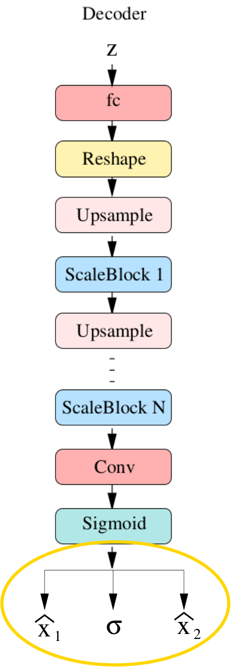
Split-VAE (SVAE) SVAE is a simple architectural variation of a traditional vae where the output is computed as a weighted sum
of two generated images , and a learned compositional map . The splitting structure facilitate the synthesis of uncorrelated latent features, usually permitting to work with latent spaces of higher dimension.
For the implementation of the encoder and the decoder we adopted a ResNet-like architecture derived from TwoStage that we already used in previous works balancing; VAEGreen. The basic component, used both for encoding and decoding is a Scale-block, described in Figure .
Encoder and decoder are essentially alternations of ScaleBlocks and downsampling/upsampling layers, as described in Figure 17.
 |
 |
| Encoder | Decoder |
Appendix B Labels for the support set
In this section we give the list of labels for elements in the support set that we used for our experiments. The precise set is not very relevant; other choices driven by the methodology described in section give similar results.
Due to memory limitations, we have been forced to restict the investigation to the first 70000 images in the CelebA dataset. This is the full list (150 elements):
[30, 58, 298, 702, 842, 873, 1779, 1809, 1844, 2590, 2719, 3888, 4114, 4223, 4550, 5659, 5718, 6058, 6108, 6128, 6175, 6244, 6705, 6815, 7499, 7679, 8225, 9457, 11254, 11282, 12367, 13077, 13371, 13993, 14193, 15390, 15711, 15817, 16505, 17186, 17458, 18250, 18283, 18582, 19080, 19175, 19612, 22505, 22633, 23173, 23199, 23308, 23511, 24231, 26431, 27169, 28270, 28401, 28433, 29453, 30248, 30269, 30619, 31741, 31795, 31836, 31978, 32272, 32770, 32828, 33332, 33613, 33669, 34024, 35804, 35823, 35882, 35944, 36483, 36926, 37374, 37534, 37538, 37572, 37682, 38194, 38483, 38677, 39232, 39267, 39424, 39901, 40405, 41464, 42969, 43035, 43199, 44054, 44252, 44589, 44798, 45930, 46259, 46693, 48128, 48786, 48839, 49498, 50345, 52454, 52516, 52673, 52753, 52834, 53071, 53308, 54937, 56128, 56492, 56693, 57844, 57927, 57942, 58020, 58089, 58162, 58389, 58947, 60359, 61004, 61180, 61374, 61495, 61530, 61794, 61878, 63535, 63891, 64328, 64342, 64663, 65041, 66277, 66321, 66663, 68027, 68753, 69274, 69750, 69936]
As it is clear from Figure 18 some images in the support set are a bit pathological: extreme poses, frequent use of accessories like hats and eyeglasses, strange illumination, etc. So the support set also provides a good test-bench to check (through inversion) the robustness and diversification of the generative model.

If required, a more “comformist” Support Set can be easily derived by reducing the threshold constraint as in Section 5.3.