Parity-encoding-based quantum computing with Bayesian error tracking
Abstract
Measurement-based quantum computing (MBQC) in linear optical systems is promising for near-future quantum computing architecture. However, the nondeterministic nature of entangling operations and photon losses hinder the large-scale generation of graph states and introduce logical errors. In this work, we propose a linear optical topological MBQC protocol employing multiphoton qubits based on the parity encoding, which turns out to be highly photon-loss tolerant and resource-efficient even under the effects of nonideal entangling operations that unavoidably corrupt nearby qubits. For the realistic error analysis, we introduce a Bayesian methodology, in conjunction with the stabilizer formalism, to track errors caused by such detrimental effects. We additionally suggest a graph-theoretical optimization scheme for the process of constructing an arbitrary graph state, which greatly reduces its resource overhead. Notably, we show that our protocol is advantageous over several other existing approaches in terms of fault-tolerance, resource overhead, or feasibility of basic elements.
I Introduction
Photonic qubits are a promising candidate for quantum computing with advantages such as long decoherence time even at room temperature. Among different encoding schemes, those of dual-rail allow one to detect photon losses by counting the total photon number and manipulate and measure single qubits via linear optical elements and photodetectors Ralph and Pryde 2010. A representative way to achieve universal quantum computing in linear optical systems is measurement-based quantum computing (MBQC) Raussendorf and Briegel 2001; Raussendorf et al. 2003 processed by single-qubit measurements on a multi-qubit graph state. In particular, a family of graph states called Raussendorf-Harrington-Goyal (RHG) lattices Raussendorf et al. 2006; Raussendorf et al. 2007; Fowler and Goyal 2009 permits universal fault-tolerant quantum computing Herr et al. 2018a; Brown and Roberts 2020; Bombin et al. 2021.
The generation of RHG lattices, which is a significant challenge for realizing fault-tolerant optical MBQC, can be done by entangling multiple small resource states with fusions of types I and/or II Browne and Rudolph 2005. Both types of fusions are not ideal in linear optics because of theoretical limitations and environmental factors such as photon losses. Fusion success rates cannot exceed 50% without additional resources Braunstein and Mann 1995 for single-photon qubits, which is far too insufficient to implement MBQC Auger et al. 2018. There exist several types of approaches to overcome this shortcoming. Some examples include (i) different types of encoding strategies with coherent states Jeong et al. 2001; Jeong and Kim 2002, hybrid qubits Omkar et al. 2020; Omkar et al. 2021, and multiphoton qubits Lee et al. 2015; Omkar et al. 2022 that significantly improve error thresholds and resource overheads Omkar et al. 2022, (ii) adding ancillary photons to boost the success rate of a type-II fusion to 75% Grice 2011; Ewert and van Loock 2014, which enables MBQC with the renormalization method Herr et al. 2018b, (iii) redundant structures added to resource states to replace a single fusion by multiple fusion attempts Fujii and Tokunaga 2010; Li et al. 2010; Li et al. 2015, and (iv) the use of squeezing for teleportation channels Takeda et al. 2013 or inline-processes Zaidi and van Loock 2013; Kilmer and Guha 2019.
Previous studies frequently treated fusion failures with bond disconnection Gimeno-Segovia et al. 2015; Zaidi et al. 2015; Pant et al. 2019 or qubit removals Auger et al. 2018; Herr et al. 2018b; Omkar et al. 2020; Omkar et al. 2022. However, to accurately evaluate the performance of computing protocols, the detrimental effects of nonideal fusions affecting nearby qubits should be analyzed more rigorously. In this work, we study how nonideal fusions corrupt stabilizers and how errors arising from such corruption can be tracked during the generation of graph states. Using a Bayesian approach and the stabilizer formalism, we can now assign error rates with strong posterior evidence from measurement data on certain qubits in the final lattice, thereby enabling much more realistic error simulations and adaptive decoding of syndromes.
We then propose a linear-optical fault-tolerant MBQC protocol termed a parity-encoding-based topological quantum computing (PTQC), which employs the parity encoding Ralph et al. 2005 and concatenated Bell-state measurement (CBSM) Lee et al. 2019. The protocol requires on-off or single-photon resolving detectors, optical switches, delay lines, and three-photon Greenberger-Horne-Zeilinger (GHZ-3) states that can be generated with linear optics. (A single-photon resolving detector discriminates between zero, one, and more than one photons entering the detector.) We analyze the loss-tolerance of the protocol while exhaustively tracking the detrimental effects of nonideal fusions. The resource overhead in terms of the number of required GHZ-3 states is also investigated. To minimize it, we introduce a graph-theoretical method for optimizing the process of constructing resource states, which is generalizable for other MBQC schemes. By comparing PTQC with three other known approaches using single-photon qubits with fusions assisted by ancillary photons, using simple repetition codes, and using redundant tree graphs, we show that our protocol is advantageous over these protocols in terms of fault-tolerance, resource overheads, or feasibility of basic elements.

I.1 Preliminaries
We denote the four Bell states by and (normalization coefficients are omitted) and call “” its sign and “” or “” its letter. An ideal Bell-state measurement (BSM) entails the measurements of and on two qubits, whose outcomes are addressed as its sign and letter outcomes, respectively. We use the polarization of photons as the degree of freedom to encode quantum information and denote the horizontally (vertically) polarized single-photon state by ().
For a given graph of qubits, a graph state is defined as the state stabilized by (that is, ) for each vertex , where and are respectively Pauli- and operators on the qubit and is the set of the vertices connected with . can be generated by placing a qubit initialized as on each vertex of and applying a controlled- gate on every pair of qubits connected by an edge in . However, since the direct implementation of a controlled- gate for photonic qubits demands multi-photon interaction, linear optical MBQC typically takes an approach to construct a graph state by merging multiple small resource graph states via fusion operations Browne and Rudolph 2005; Kieling et al. 2007; Fujii and Tokunaga 2010; Li et al. 2010; Gimeno-Segovia et al. 2015; Li et al. 2015; Zaidi et al. 2015; Herr et al. 2018b; Pant et al. 2019; Omkar et al. 2020; Omkar et al. 2022.
Among the two types of fusions Browne and Rudolph 2005, we only consider type II since type I may convert photon losses into unheralded errors Li et al. 2015. A type-II fusion is done by measuring and on two qubits. In practice, it is realized by applying the Hadamard gate on one of the qubits and then performing a BSM on them. For two qubits , if and are disjoint, the effect of a fusion on the qubits is to connect (disconnect) every possible pair of disconnected (connected) qubits, one from and the other from , up to several Pauli- operators determined by the BSM outcome. These Pauli- operators are compensated by updating the Pauli frame Knill 2005 classically. This effect can be checked by tracking stabilizers, as shown in the example of Fig. 1(a). Here, the stabilizer (colored in green) before the fusion is transformed into after the fusion, where is the sign outcome of the BSM if the Hadamard gate is applied on qubit . The other two stabilizers (colored in purple) and that commute with the fusion can be transformed in similar ways. Consequently, the marginal state on the unmeasured qubits is equal to the merged graph state up to several Pauli- operators, as presented in Fig. 1(b).
We consider errors of qubits in the “vacuum” measured in the -basis, which occupies most of the area in the RHG lattice Raussendorf et al. 2006; thus, -errors do not affect the results. Henceforth, every error mentioned is a -error.
II Results
II.1 Bayesian error tracking for nonideal fusions

We now introduce the methodology to track the errors caused by nonideal fusions. Let us revisit the example in Fig. 1, supposing that the qubits are single-photon polarization ones and there are no photon losses. Then a BSM can discriminate between only two Bell states (say, ) among the four without additional resources Lütkenhaus et al. 1999; see Fig. 2 for the scheme. The intact final state is obtained only when the BSM succeeds. When the BSM fails (which is heralded), is determined while is left completely ambiguous. In other words, the posterior probability that the input state is for the obtained photodetector outcomes is equal for both signs (), assuming that the four Bell states have the same prior probability. This assumption can be justified by the fact that the marginal state on qubits and before the fusion is maximally mixed; see Supplementary Note 1 for the proof. Therefore, we fix the value of while randomly assign that of . Then, the operator , which is originally a stabilizer of , gives randomly when it is measured after the failed BSM. Whereas, the other two stabilizers and are left undamaged. The key point is that this situation is equivalent to a 50% chance of an erroneous qubit 1 in in terms of stabilizer statistics. In other words, both situations give the same statistics if the stabilizers of are measured; thus, every process in MBQC described with the stabilizer formalism works in the same way.
Generally, a nonideal BSM gives one of the possible outcomes and the posterior probability of each Bell state for the outcome can be calculated with the Bayesian theorem, assuming the equal prior probabilities of the Bell states. Accordingly, the Bell state with the highest posterior probability is selected as the result of the BSM, and the probability () that the selected sign (letter) is wrong can be obtained as well. These error probabilities are “propagated” into nearby qubits in a way that the stabilizer statistics are preserved. For example, if the fusion in Fig. 1 is nonideal in such a way, it is equivalent to qubit 1 having an error with probability and qubits and having correlated errors with probability . We term a qubit with a nonzero error rate deficient.
Additionally, if a qubit participating in a fusion is erroneous, this error is propagated to the qubits on the opposite side. For example, an erroneous qubit 0 in Fig. 1 induces an error in the measurement, which is equivalent to erroneous qubits and .
The above error tracking methodology can be utilized for accurate and effective error simulations. The method can precisely locate qubits affected by unsuccessful fusions, which is closer to reality than simple bond disconnection or qubit removal. Since unsuccessful fusions are now regarded as Pauli error sources, we no longer need lattice deformation and the construction of supercheck operators Barrett and Stace 2010; Auger et al. 2018. Instead, the error probabilities on individual qubits are employed for decoding syndromes in an adaptive manner (with decoders such as the weighted minimum-weight perfect matching one), which may be particularly effective if the probabilities are between 0 and since regarding such errors as just removal of qubits is a loss of information.
II.2 Building an RHG lattice

An RHG lattice can be built with two types of linear three-qubit graph states called central and side microclusters Gimeno-Segovia et al. 2015; Herr et al. 2018b. The process is composed of two steps (see Fig. 3): In step 1, a central microcluster and two side microclusters are merged by two fusions to form a five-qubit graph state named a star cluster composed of one central qubit and four side qubits. In step 2, the side qubits of star clusters are fused to form an RHG lattice. Eventually, the lattice includes only the central qubits, which are measured in appropriate bases for MBQC. For step 2, we consider two options: (i) Star clusters with successful step-1 fusions may be post-selected, or (ii) all generated star clusters are used regardless of the fusion results. The locations of the Hadamard gates during fusions (called -configuration) may be chosen arbitrarily. Here, we define two specific -configurations: Hadamard-in-center (HIC) and Hadamard-in-side (HIS). In the HIC (HIS) configuration, the Hadamard gates in step 1 are applied on qubits in the central (side) microclusters, as shown in Fig. 3. Whereas the Hadamard gates in step 2 are arranged in the same pattern for both configurations.
Nonideal fusions during lattice building render some central qubits in the final lattice deficient, as shown in Fig. 3 when the HIC configuration is used. When the HIS configuration is used, the positions of and in the figure are swapped. Note that errors in the side qubits are propagated to the nearest central qubits after step 2. Correlation between the sign and letter errors of a fusion, if any, can be neglected if the primal and dual lattices are considered separately, since these errors respectively affect primal and dual Raussendorf et al. 2006 qubits (or vice versa).
II.3 Noise model
For analyzing the following linear optical quantum computing protocols, we consider a noise model where each photon suffers an independent loss with probability , which arises from imperfections throughout the protocol: GHZ-3 states (which are initial resource states), delay lines, optical switches, and photodetectors. We assume that noise that cannot be modeled with photon losses such as dark counts is negligible. Note that not only nonideal fusions but also photon losses in central qubits, which are detectable by on-off detectors, may incur deficiency. If the measurement outcome of a central qubit cannot be determined due to photon losses, we select the outcome randomly and assign an error rate of 50% to the qubit.
II.4 Parity-encoding-based topological quantum computing
We introduce the new linear-optical parity-encoding-based topological quantum computing (PTQC) protocol, where fusion success rates are boosted by using multiphoton qubits for all qubits that participate in fusions and single-photon polarization encoding is used for central qubits. The parity encoding Ralph et al. 2005 is employed for the multiphoton qubits, which are fused by CBSM Lee et al. 2019. On-off or single-photon resolving detectors are used as photodetectors, and GHZ-3 states, which can be generated linear-optically Varnava et al. 2008, are regarded as basic resource states. The parity encoding defines a basis as
| (1) |
where
| (2) |
The Hilbert space has a hierarchical structure composed of three levels: the lattice, block, and physical levels with respective bases , , and . In the original CBSM scheme Lee et al. 2019, a BSM of a certain level is decomposed into multiple BSMs of one level below. Our current CBSM scheme slightly differs from the original one in the following two areas: (i) We consider two types of photodetectors: single-photon resolving and on-off detectors. A physical-level BSM can discriminate between a photon loss and failure only if single-photon resolving detectors are used. (ii) The letter outcome of a lattice-level BSM is obtained by a weighted majority vote of block-level letter outcomes. See the Methods section for details of the CBSM scheme and its error rates.

For practical reasons, we consider generating post- microclusters (that is, the states obtained by applying several lattice-level Hadamard gates on microclusters) directly from GHZ-3 states, instead of generating microclusters first and then applying the lattice-level Hadamard gates for the fusions. Figure 4(a) depicts the central and side post- microclusters for the HIC and HIS configurations. A post- microcluster can be generated up to several physical-level Hadamard gates by performing physical-level BSMs or fusions (referred to as merging operations) between multiple GHZ-3 states according to a predetermined merging graph, as shown in the example of Fig. 4(b). Note that the merging graph may be not unique for a post- microcluster. However, each merging operation has a low success rate of less than or equal to 50%, which may lead to extensive usage of GHZ-3 states for generating a post- microcluster successfully. Thus, the generation process, which is determined by the merging graph and the order of the merging operations, should be adjusted carefully to minimize the resource overhead. To optimize the merging order, our protocol utilizes a graph edge coloring algorithm, based on the idea that merging operations for non-adjacent edges can be performed simultaneously. See the Methods section for details of the structures of post- microclusters, their generation, and the resource optimization problem.
For error simulations, we consider the logical identity gate with the length of unit cells along the simulated time axis, where is the code distance. All the fusion outcomes are sampled from appropriate probability distributions, and the corresponding error rates are assigned to individual central qubits according to the process described earlier. These error rates are exploited when decoding syndromes by the weighted minimum-weight perfect matching in the PyMatching package Higgott 2021. The loss thresholds are calculated by finding the intersections of logical error rates for and . The resource overhead of PTQC is quantified by the average total number of GHZ-3 states to achieve a target logical error rate of for the logical identity gate of , which depends on the photon loss rate . See Supplementary Notes 2 and 3 for the detailed methods of error simulations and resource calculations, respectively.
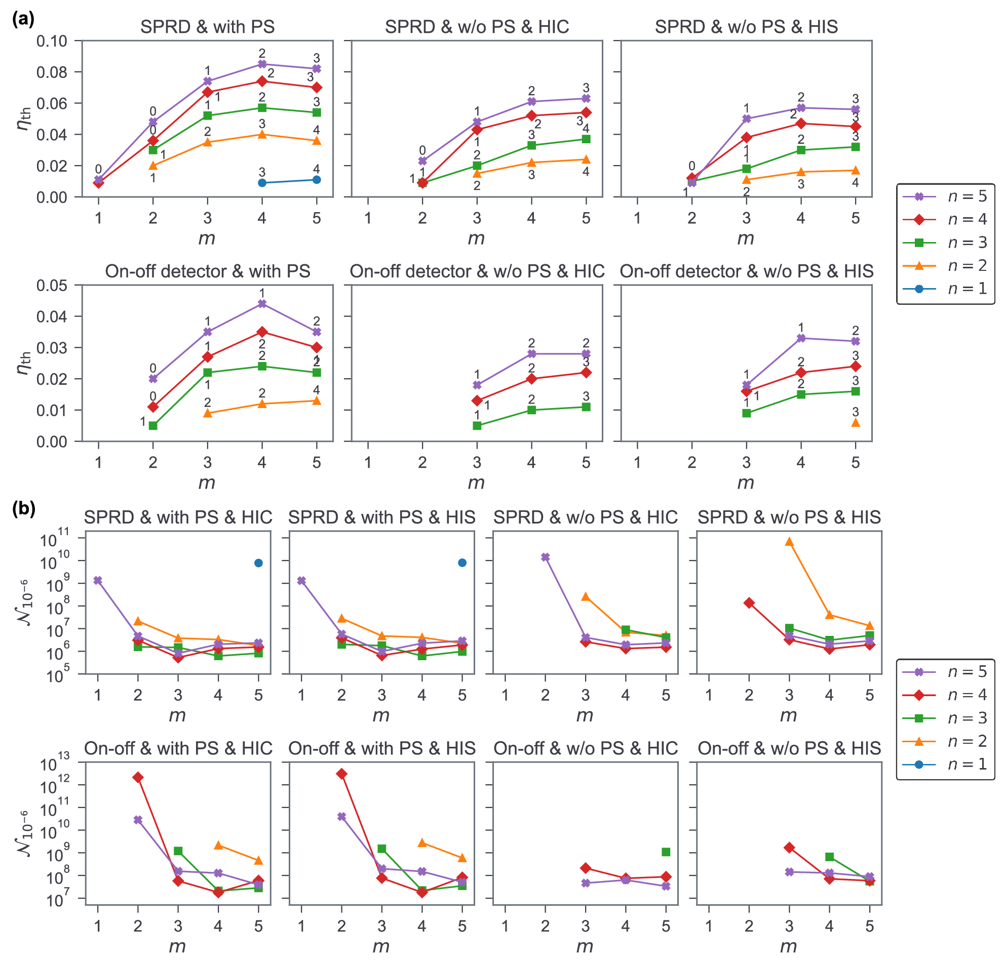

The simulation results of the loss thresholds and the resource overheads (quantified by ) are respectively presented in Figs. 5(a) and (b) for the two types of photodetectors, the two options for the post-selection of star clusters, and the two -configurations. Figure 5(a) shows that, if single-photon resolving detectors are used, reaches up to 8.5% () when star clusters are post-selected and up to 6.3% (, HIC) when they are not. If on-off detectors are used, reaches up to 4.4% () when star clusters are post-selected and up to 3.3% (, HIS) when they are not. The post-selection of star clusters increases the photon loss thresholds by about . From Fig. 5(b), it is observed that the protocol using single-photon resolving detectors is most resource-efficient with (, HIC) when star clusters are post-selected and with (, HIS) when they are not. If on-off detectors are used, the protocol is most resource-efficient with (, HIC) when star clusters are post-selected and with (, HIC) when they are not. It is worth noting that, compared to the protocol without the post-selection, the protocol with it requires fewer GHZ-3 states to achieve a target logical error rate. In other words, further fault-tolerance obtained by using only successfully-generated star clusters leads to a positive overall effect that surpasses the negative effect caused by the increase in the number of required GHZ-3 states for one central qubit in the final lattice.
Additionally, Fig. 6 presents the photon loss thresholds as a function of when is fixed to or variable as , which is used to calculate . aIt shows that at least about 400 GHZ-3 states are required per central qubit for PTQC to work. The explicit information of the data points along the upper envelope lines in the figure is presented in Supplementary Table 1.
II.5 Comparison with other approaches
We now compare the PTQC protocol with three other known approaches for linear optical quantum computing: (i) using single photons for all qubits with fusions assisted by ancillary photons, (ii) using simple repetition codes, and (iii) attaching redundant tree structures to replace a single fusion by multiple fusion attempts. We show evidence that PTQC is more efficient than these approaches.
We first consider the approach of (i) that uses single photons for all qubits with fusions assisted by ancillary photons Ewert and van Loock 2014, which has been widely studied in the context of ballistic quantum computing Gimeno-Segovia et al. 2015; Zaidi et al. 2015; Herr et al. 2018b; Pant et al. 2019. In these works, non-RHG lattices are considered except for Ref. Herr et al. 2018b; however, RHG lattices should be used to enable a solid error correction, as also mentioned in Refs. Gimeno-Segovia et al. 2015; Pant et al. 2019. Moreover, in these works, the detrimental effects of failed fusions corrupting nearby qubits are not treated comprehensively; instead, they (except Ref. Herr et al. 2018b) regard a fusion failure as removing the corresponding edge and mainly focus on finding percolation thresholds.
By analyzing the approach of (i) with our methodology for handling nonideal fusions, we can show that should be less than about 10% (1%) even if is only 1% when star clusters are (are not) post-selected; see Supplementary Note 4 for the detailed methods and results. The failure rate of can be achieved by using the BSM scheme of in Ref. Ewert and van Loock 2014 where . It requires multiple photon-number resolving detectors (PNRDs) resolving up to 16 photons and specific four- and eight-photon ancillary states that are conjectured to be impossible to obtain from single photons with linear optics Ewert and van Loock 2014. Moreover, our simulation does not consider the imperfectness of ancillary states and additional PNRDs; if they are considered, the requirements will be even stricter. Therefore, it may be highly demanding to implement this MBQC protocol with linear optics. We note that there is a possibility that the lattice renormalization method in Ref. Herr et al. 2018b makes the protocol less demanding, which is worth investigating in future works. However, the method has a shortcoming that the renormalized lattice may be significantly smaller than the original lattice; namely, about photons are consumed to generate one node Herr et al. 2018b.
Next, we consider the approach of (ii) that uses simple repetition codes, which is covered in our previous work Omkar et al. 2022. In Ref. Omkar et al. 2022, the photon loss thresholds and resource overheads are analyzed in detail, but a rigorous analysis of the effects of nonideal fusions like that done for PTQC is lacking. It is observed that the recalculated photon loss thresholds are lower than the values reported in Omkar et al. 2022, which shows that PTQC is much more loss-tolerant than this approach. For example, if each central qubit consists of two photons, the obtained optimal photon loss threshold is 0.97% (0.40%) when star clusters are (are not) post-selected, while the reported value is 3.3% (3.1%). Moreover, encoding central qubits with the repetition code does not improve the performance significantly. See Supplementary Note 5 for details.
Lastly, we compare PTQC with the approach of (iii) that utilizes redundant tree structures on graph states. Such an approach also has been actively investigated Fujii and Tokunaga 2010; Li et al. 2010; Li et al. 2015, among which Ref. Li et al. 2015 presents the current most advanced version of the protocol where an RHG lattice is constructed by entangling multiple GHZ-3 states like PTQC. There, at least photodetectors are required per data qubit to achieve a positive photon loss threshold with single-photon resolving detectors, while PTQC requires at least photodetectors per data qubit (see the Methods section for the calculation). Hence, PTQC shows about a twofold improvement in resource efficiency compared to the protocol in Ref. Li et al. 2015. Furthermore, we have shown that PTQC also operates with on-off detectors, while the protocol in Ref. Li et al. 2015 is currently unclear whether it is possible. Nevertheless, further work will be required to compare their performance (especially their fault-tolerance) rigorously and comprehensively.
III Discussion
In this work we address the problem of overcoming the negative effects of nonideal fusions and photon losses during linear-optical measurement-based quantum computing (MBQC). We first introduced a Bayesian methodology for tracking errors caused by nonideal fusions during the construction of graph states, which enables accurate and effective error simulations. We then proposed the parity-encoding-based topological quantum computing (PTQC) protocol that uses the parity encoding and concatenated Bell-state measurement, which turns out to have a high loss threshold of at most . Moreover, logical error rates near can be achieved using about or fewer three-photon Greenberger-Horne-Zeilinger states (GHZ-3) states in total when the photon loss rate is 1%, which outperforms other known linear optical computing protocols Omkar et al. 2022. We presented comprehensive and systematic methods to construct a graph state from GHZ-3 states, including the graph-theoretical algorithm that can minimize the resource overhead efficiently.
Additionally, we investigated three other known approaches that respectively use single-photon qubits with fusions assisted by ancillary photons, simple repetition codes, and redundant tree graphs. We verified that the first two are highly demanding compared to PTQC due to low photon loss thresholds or hard-to-implement requirements such as photodetectors that can resolve many photons. Compared to the third approach, we showed that PTQC has a twofold improvement in terms of the resource overhead required for the loss threshold to be positive, although additional work will be necessary to compare their fault-tolerance as well.
One may apply the Bayesian error tracking method to other encoding schemes or decoding algorithms (such as the union-find decoder Delfosse and Nickerson 2021) to improve fault-tolerance or resource overheads. More careful consideration of component-wise errors, including both heralded photon losses and unheralded errors (such as dark counts on photodetectors), shall give rise to more realistic analyses. Resource analysis will be more comprehensive if other factors such as the number of optical switches or the lengths of delay lines are considered. In particular, one trial of CBSM may require optical switches to change the types (, , and ) of the physical-level BSMs. Our graph-theoretical optimization scheme for generating graph states can be applied to arbitrary graph states as well as microclusters for PTQC. It will be interesting future work to investigate the resource reduction effect of this scheme for various MBQC protocols or other applications of graph states such as quantum repeaters. Lastly, our methods may be generalized to fusion-based quantum computing Bartolucci et al. 2021 that is attracting attention recently, or other MBQC protocols such as the color-code-based one Lee and Jeong 2022.
IV Methods
In this section, we describe the details of the PTQC protocol including the CBSM scheme, the closed-form expressions of error probabilities, the method to generate post- microclusters, and the resource optimization problem.
IV.1 Bell states for the parity encoding
For the lattice, block, and physical levels of the parity encoding, the Bell states are respectively defined as
where , , and are defined in Eqs. (1) and (2).
| The Bell states of each level can be decomposed into those of one level below as follows: | ||||
| (3a) | ||||
| (3b) | ||||
| (3c) | ||||
| (3d) | ||||
| where means the summation of all the permutations of the tensor products inside the bracket. Therefore, a BSM can be performed in a concatenated manner: A lattice-level BSM () is done by block-level BSMs (’s), each of which is again done by physical-level BSMs (’s). We refer to the sign (letter) result obtained from a lattice-, block-, or physical-level BSM as the lattice-, block-, or physical-level sign (letter), respectively. | ||||
IV.2 Original CBSM scheme
We review the original CBSM scheme of the parity encoding in Ref. Lee et al. 2019. A can discriminate between only two among the four Bell states. Three types of ’s (, , and ) are considered, which discriminate between , , and , respectively. can be implemented by the process in Fig. 2, which can be modified to implement instead by adding a wave plate on each input line just before the first PBS. If the wave plate on the second input line is removed in the setting for , is executed alternatively. A has four possible outcomes: two successful cases (e.g., for , and ), “failure,” and “detecting a photon loss.” Failure and loss can be distinguished by the number of total photons detected by the photon detectors. Since two photons may enter a single detector, it is assumed that single-photon resolving detectors are used. Note that, even in the failure cases, either sign or letter still can be determined. (For example, even if a fails, we can still learn that the letter is .) On the other hand, if it detects a loss, we can get neither a sign nor a letter.
A is done by -times of ’s. Each block is composed of photons, thus we consider pairs of photons selected respectively in the two blocks. The types of the ’s are selected as follows: First, is performed on each pair of photons in order until it either succeeds, detects a loss, or consecutively fails times, where is a predetermined number. Then a sign is selected by the sign of the last outcome if it succeeds or selected randomly if it fails or detects a loss. After that, ’s are performed for all the left pairs of photons.
The block-level sign (letter) is determined by the physical-level signs (letters) of the ’s. In detail, the block-level sign is chosen (i) to be the same as if the last succeeds or any succeeds, and (ii) to be the opposite of if the last does not succeed and any fails. (iii) Otherwise (namely, if the last does not succeed and all the ’s detect losses), the block-level sign is not determined. The block-level letter is determined only when all the physical-level letters are determined, namely, when no losses are detected and all ’s succeed. For such cases, the block-level letter is () if the number of in the results is even (odd).
Next, a is done by -times of ’s. The lattice-level sign is determined only when all the block-level signs are determined; it is if the number of in the results is even and it is if the number is odd. The lattice-level letter is equal to any determined block-level letter. Thus, if all ’s cannot determine letters, the lattice-level letter is not determined as well.
IV.3 Modified CBSM scheme for PTQC
In our PTQC protocol, we consider using either single-photon resolving or on-off detectors. The CBSM scheme should be slightly modified for this case.
Since failure and loss cannot be distinguished, a now has three possible outcomes: two successful cases and failure. Consequently, in a , ’s are performed until it either succeeds or consecutively fails times. The way to determine the block-level sign and letter is the same as the original scheme, except that case (iii) when determining the sign no longer occurs. The biggest difference from the original scheme is that the determined sign and letter may be wrong. These error probabilities are presented in the next subsection.
In a , the lattice-level sign is determined from the block-level signs by the same method as the original scheme, although it may be wrong with a nonzero probability as well. On the other hand, the lattice-level letter is not determined by a single block-level letter unlike the original scheme; instead, we use a weighted majority vote of block-level letters. The weight of each block-level letter is given as , where is the probability that the block-level letter is wrong. This weight factor is justified as follows: Let () denote the set of the indices of block pairs where the block-level letters are (). Assuming that the two lattice-level letters ( and ) have the same prior probability, we get
where and are respectively the letter error probability and the weight of the th block. Note that the third equality comes from the fact that a lattice-level Bell state is decomposed into block-level Bell states of the same letter, as shown in Eqs. (3a) and (3b).
IV.4 Error probabilities of a CBSM under a lossy environment
We here present the possible outcomes of a CBSM using either single-photon resolving or on-off detectors and the corresponding error probabilities . We denote , which is the probability that a does not detect photon losses. It is assumed that the four Bell states have the same prior probabilities; namely, the initial marginal state on qubits 1 and 2 before suffering losses is the equal mixture of four lattice-level Bell states, which is justified in Supplementary Note 1. For a or , to avoid confusion, we use the term “outcome” to indicate the tuple of the outcomes of the ’s constituting the or , and use the term “result” to indicate one of the four Bell states that gives the largest posterior probability under its outcome. Note that the result of a BSM may be not deterministically determined by its outcome; if multiple Bell states have the same posterior probability, one of them is randomly selected as the result.
The case using single-photon resolving detectors is analyzed in Ref. Lee et al. 2019 and we here review the contents to be self-contained. The outcome of a is included in one of the following three cases: (Success) Both the sign and letter are identified if no losses are detected and all the ’s succeed. (Failure) Neither sign nor letter is identified if no ’s succeed and all ’s detect losses. (Sign discrimination) Only the sign is identified if otherwise. The block-level sign (or letter) is selected randomly if it is not identified. The probabilities of these cases are respectively
For a , let () denote the number of successful (failed) ’s. The lattice-level letter is identified if (namely, if at least one block-level letter is identified) and the sign is identified if (namely, if all block-level signs are identified). Hence, the outcome of a is included in one of the following four events:
The sign and letter error probabilities of the for each event are for , for , for , and for . The probabilities of the events are respectively given as
| (4) | ||||
We now consider using on-off detectors for fusions. Each outcome of a is uniquely identified by a triple , where is the number of failed ’s, is the sign chosen by the successful th (if ) or randomly (if ), and is an -element tuple composed of “,” “,” and “” (failure) indicating the outcomes of the ’s from the th to the the last. (If , the first component of is always , and the other components are determined by the ’s. If , all the components are determined by the ’s.) Let for denote the number of in . Then a outcome is included in one of the following events:
| (5) | ||||
where is the set of all possible outcomes. Note that the events , , and correspond to success, failure, and sign discrimination when . For each event in Eq. (5), its sign and letter error probabilities and the probability that the event occurs are given as follows (see Supplementary Note 6 for their derivation):
| (6) | ||||
A possible outcome of a corresponds to an -tuple of events composed of (), , and , which can be regarded as an independent event for the outcomes of the . The probability that an event occurs is
| (7) |
and the sign and letter error probabilities of are respectively
where is the number of ’s in , , and is if and 0 if . See Supplementary Note 6 for their derivation.
IV.5 Generation of post- microclusters

In this subsection, we first present the physical-level graphs of post- microclusters for PTQC and then describe the method to generate them. A post- microcluster, which is composed of three lattice-level qubits or two of them and one photon (physical-level qubit), can be regarded as a graph state of photons up to several physical-level Hadamard gates. The graph of this graph state, called the physical-level graph of the post- microcluster, is visualized in Fig. 7 for each post- microcluster; see Supplementary Note 7 for their derivation. Here, the squares (circles) indicate lattice-level (physical-level) qubits. If a square (circle) is filled with black, it means that the lattice-level (physical-level) Hadamard gate is applied on the qubit after the involved edges are connected. Recurrent subgraphs are abbreviated as blue dashed squares or circles with numbers; see Fig. 7(b) for the detailed interpretation of these notations.
We now depict the ways to generate a specific post- microcluster from GHZ-3 states. We first describe a straightforward method and then adjust or generalize it. The final method can be summarized as follows:
- 1.
Determine a merging graph for the post- microcluster that we want to create by the algorithm presented below. Each edge of is labeled as either “internal” or “external.”
- 2.
For each vertex in , Prepare a GHZ-3 state .
- 3.
For each edge in that connects and , perform a BSM (fusion) on two photons selected respectively from and if is an internal (external) edge. The order of the operations does not matter.
We define the GHZ- state for an integer by the state . Note that it is a state obtained from a graph state with a star graph (where the number of vertices is ) by applying Hadamard gates on all the leaves of the graph; namely,
We refer to the first photon of the above expression as the root photon of the state (which can be chosen arbitrarily) and the other photons as its leaf photons.

If a BSM is performed on the root photon of a GHZ- state and a leaf photon of a GHZ- state, the resulting state on the remaining photons is a GHZ- state; see Fig. 8(a) for an example. Thus, an arbitrary GHZ state can be constructed by performing BSMs on multiple GHZ-3 states appropriately. On the other hand, if a fusion is performed on two leaf photons selected respectively from GHZ- and GHZ- states, the resulting state is no longer a GHZ state, but it is a graph state (up to some Hadamard gates) with a graph containing a vertex with degree , a vertex with degree , and multiple vertices with degree one; see Fig. 8(b) for an example. (The degree of a vertex means the number of edges connected to .)
Combining the above facts, a post- microcluster (or an arbitrary graph state) with the physical-level graph can be generated from GHZ-3 states up to physical-level Hadamard gates in the following way: For each vertex of with a degree larger than one, prepare a state through BSMs on GHZ-3 states. Then, for each edge of , perform a fusion on two photons selected respectively from and . We refer to each BSM or fusion during this process as a merging operation.

However, the above method still has room for improvement. The physical-level graphs in Fig. 7 can be decomposed into multiple components that are combined by fusions through the process shown in Fig. 9. Here, each recurrent subgraph connected with multiple vertices is separated and connected with only one vertex. The decomposition of different post- microclusters is explicitly presented in Supplementary Figure 8. To generate a post- microcluster, we prepare the individual components first by the aforementioned method, then merge them through fusions. This process may greatly reduce the number of required merging operations since the number of edges decreases as shown in Fig. 9.

Furthermore, we can generalize the method using the fact that every merging operation commutes with each other. That is, even if all the fusions and BSMs in the above process are performed in an arbitrary order, the final state does not vary (up to the change of the Pauli frame). To systematically address this feature, we define a merging graph of a post- microcluster or one of its components by a graph in which the vertices correspond to initial GHZ-3 states and the edges indicate the merging operations between them required to generate the state. Each edge of a merging graph is either internal or external that corresponds to BSMs or fusions, respectively.
A merging graph of a component can be constructed by the following method starting from its physical-level graph (see Fig. 10 for two examples): First, for each vertex satisfying in the physical-level graph, replace it with new vertices connected by internal edges in series with each other. This process means decomposing a GHZ- state into GHZ-3 states. The edges originally connected to are distributed to the new vertices in a way that every new vertex is connected to three or fewer edges. Then there is only one vertex connected to two edges, which is called the seed vertex of . This seed vertex means that one photon in the corresponding GHZ-3 state does not participate in any merging operation and remains in the final state. Lastly, the merging graph is obtained by removing all the vertices with degree one. See Supplementary Note 8 for a stricter step-by-step description of the method.
The merging graph of a post- microcluster is constructed by combining the merging graphs of its components. That is, for each fusion between different components, the corresponding seed vertices in the merging graphs are connected by an external edge. Then we finally get the method summarized at the beginning of this subsection.
IV.6 Optimization of resource overheads
The process of generating a post- microcluster described above is determined by two factors: the merging graph and the order of the merging operations. Here, we discuss their optimization for minimizing resource overhead. The merging graph is selected randomly by the algorithm in Supplementary Note 8. Based on it, we determine the order of the merging operations through an algorithm found heuristically and calculate the expected number of GHZ-3 states required to generate the state. We repeat this process for a large enough number to obtain as low resource overhead as possible. and can be calculated by using the obtained optimal resource overheads; see Supplementary Note 3 for details.
During the generation process, performing each merging operation can be regarded as contracting the corresponding edge, which means removing the edge, merging the two vertices that it previously joined into a new vertex , and reconnecting all the edges that were connected to and with . Here, each vertex indicates a connected subgraph (a group of entangled photons) of the intermediate graph state. We assign a “weight” (which is initialized to 1) on each vertex , which is the average number of GHZ-3 states required to generate the connected subgraph. If the edge between two vertices and are contracted, the new vertex has the weight of
| (8) |
where the factor is the inverse of the success probability of the merging operation. By repeating this process, the post- microcluster is obtained when there is only one vertex left, whose weight is equal to .
To find an optimal order of merging operations, we use the following strategy:
- 1.
Find the set of edges with the smallest weight, where the weight of an edge is defined as .
- 2.
Using an edge coloring algorithm, allocate “colors” to all edges so that different edges sharing a vertex have different colors and as few colors as possible are used.
- 3.
Partition into disjoint subsets by the colors of the edges. Find the largest subset among them. If such a subset is not unique, choose one randomly.
- 4.
Contract each edge in in an arbitrary order.
- 5.
Repeat all the above steps until only one vertex is left.
The strategy is based on the following two intuitions: First, it is better to merge vertices with small weights first, since if . Secondly, it is better to perform merging operations in parallel as much as possible. Such a set of edges can be found by the edge coloring algorithm. For our results, we have used the function coloring.greedy_color in NetworkX package Hagberg et al. 2008 with the strategy largest_first. (Since the function performs vertex coloring, we input the line graph of into the function.)
In Supplementary Note 9, we show an evidence that this optimizing strategy is indeed highly effective in terms of both the optimality of the calculated overhead and searching time, by comparing its performance with those of its variants constructed by omitting or altering specific steps. We conjecture that this strategy is powerful for generating general graph states as well as those for PTQC, which will be worth investigating.
IV.7 Conversion of resource measures
We here address the conversion of resource measures for a fair comparison between PTQC and the protocol in Ref. Li et al. 2015. In Ref. Li et al. 2015, resource overheads are quantified by the number of photodetectors required per central qubit, not the number of GHZ-3 states we have used, thus conversion between them is necessary for a fair comparison. In PTQC, detectors are used when generating GHZ-3 states, applying physical-level BSMs, and measuring central qubits. We suppose that GHZ-3 states are generated by the scheme proposed in Ref. Varnava et al. 2008 like the protocol in Ref. Li et al. 2015. The scheme uses six detectors to generate a single GHZ-3 state and succeeds with probability ; thus, generating one GHZ-3 state requires 192 detectors. (If it is allowed to use photodetectors repeatedly during the generation of each GHZ-3 state, only six detectors are required per GHZ-3 state. However, we ignore this option to be consistent with Ref. Li et al. 2015.) Next, four detectors are used for one physical-level BSM (see Fig. 2). Counting the number of physical-level BSMs per central qubit is not simple, but we can get its upper bound as , which is half the number of total photons in all GHZ-3 states except one photon in the central qubit. Lastly, two detectors are used for the two polarization modes when measuring a central qubit. In total, detectors are required per data qubit in PTQC. Since is required for a positive photon loss threshold (see Fig. 6), should be at least about .
Data Availability
All the numerical data used to generate the figures are available from the corresponding author upon reasonable request.
Code Availability
The Python codes used for numerical simulations are available from the corresponding author upon reasonable request.
Author Contributions
All authors (S.H.L., S.O., Y.S.T., and H.J.) contributed to developing the main idea. S.H.L. concretized the idea with mathematical analysis, wrote the codes, and ran numerical simulations. S.O. suggested important ideas on resource analysis. Y.S.T. checked the results and H.J. supervised the project. All authors helped write the manuscript.
Competing Interests
The authors declare no competing interests.
Acknowledgements
This work was supported by the National Research Foundation of Korea (NRF) grants funded by the Korean government (Grant Nos. NRF-2020R1A2C1008609, NRF-2019R1A6A1A10073437, NRF-2022M3E4A1076099, and 2022M3K4A1097117) via the Institute of Applied Physics at Seoul National University, and by the Institute of Information & Communications Technology Planning & Evaluation (IITP) grant funded by the Korea government (MSIT) (IITP-2021-0-01059 and IITP-2022-2020-0-01606). We thank Kamil Bradler, Brendan Pankovich, Angus Kan, and Alex Neville for insightful discussions.
References
- Ralph and Pryde (2010) T. C. Ralph and G. J. Pryde, Chapter 4 - Optical Quantum Computation (Elsevier, 2010) pp. 209–269.
- Raussendorf and Briegel (2001) R. Raussendorf and H. J. Briegel, A one-way quantum computer, Phys. Rev. Lett. 86, 5188 (2001).
- Raussendorf et al. (2003) R. Raussendorf, D. E. Browne, and H. J. Briegel, Measurement-based quantum computation on cluster states, Phys. Rev. A 68, 022312 (2003).
- Raussendorf et al. (2006) R. Raussendorf, J. Harrington, and K. Goyal, A fault-tolerant one-way quantum computer, Ann. Phys. 321, 2242 (2006).
- Raussendorf et al. (2007) R. Raussendorf, J. Harrington, and K. Goyal, Topological fault-tolerance in cluster state quantum computation, New J. Phys. 9, 199 (2007).
- Fowler and Goyal (2009) A. G. Fowler and K. Goyal, Topological cluster state quantum computing, Quantum Info. Comput. 9, 721–738 (2009).
- Herr et al. (2018a) D. Herr, A. Paler, S. J. Devitt, and F. Nori, Lattice surgery on the Raussendorf lattice, Quantum Sci. Technol. 3, 035011 (2018a).
- Brown and Roberts (2020) B. J. Brown and S. Roberts, Universal fault-tolerant measurement-based quantum computation, Phys. Rev. Research 2, 033305 (2020).
- Bombin et al. (2021) H. Bombin, C. Dawson, R. V. Mishmash, N. Nickerson, F. Pastawski, and S. Roberts, Logical blocks for fault-tolerant topological quantum computation, arXiv preprint arXiv:2112.12160 (2021).
- Browne and Rudolph (2005) D. E. Browne and T. Rudolph, Resource-efficient linear optical quantum computation, Phys. Rev. Lett. 95, 010501 (2005).
- Braunstein and Mann (1995) S. L. Braunstein and A. Mann, Measurement of the Bell operator and quantum teleportation, Phys. Rev. A 51, R1727(R) (1995).
- Auger et al. (2018) J. M. Auger, H. Anwar, M. Gimeno-Segovia, T. M. Stace, and D. E. Browne, Fault-tolerant quantum computation with nondeterministic entangling gates, Phys. Rev. A 97, 030301(R) (2018).
- Jeong et al. (2001) H. Jeong, M. S. Kim, and J. Lee, Quantum-information processing for a coherent superposition state via a mixedentangled coherent channel, Phys. Rev. A 64, 052308 (2001).
- Jeong and Kim (2002) H. Jeong and M. S. Kim, Efficient quantum computation using coherent states, Phys. Rev. A 65, 042305 (2002).
- Omkar et al. (2020) S. Omkar, Y. S. Teo, and H. Jeong, Resource-efficient topological fault-tolerant quantum computation with hybrid entanglement of light, Phys. Rev. Lett. 125, 060501 (2020).
- Omkar et al. (2021) S. Omkar, Y. S. Teo, S.-W. Lee, and H. Jeong, Highly photon-loss-tolerant quantum computing using hybrid qubits, Phys. Rev. A 103, 032602 (2021).
- Lee et al. (2015) S.-W. Lee, K. Park, T. C. Ralph, and H. Jeong, Nearly deterministic bell measurement with multiphoton entanglement for efficient quantum-information processing, Phys. Rev. A 92, 052324 (2015).
- Omkar et al. (2022) S. Omkar, S.-H. Lee, Y. S. Teo, S.-W. Lee, and H. Jeong, All-photonic architecture for scalable quantum computing with greenberger-horne-zeilinger states, PRX Quantum 3, 030309 (2022).
- Grice (2011) W. P. Grice, Arbitrarily complete Bell-state measurement using only linear optical elements, Phys. Rev. A 84, 042331 (2011).
- Ewert and van Loock (2014) F. Ewert and P. van Loock, -Efficient Bell measurement with passive linear optics and unentangled ancillae, Phys. Rev. Lett. 113, 140403 (2014).
- Herr et al. (2018b) D. Herr, A. Paler, S. J. Devitt, and F. Nori, A local and scalable lattice renormalization method for ballistic quantum computation, npj Quantum Information 4, 1 (2018b).
- Fujii and Tokunaga (2010) K. Fujii and Y. Tokunaga, Fault-tolerant topological one-way quantum computation with probabilistic two-qubit gates, Phys. Rev. Lett. 105, 250503 (2010).
- Li et al. (2010) Y. Li, S. D. Barrett, T. M. Stace, and S. C. Benjamin, Fault tolerant quantum computation with nondeterministic gates, Phys. Rev. Lett. 105, 250502 (2010).
- Li et al. (2015) Y. Li, P. C. Humphreys, G. J. Mendoza, and S. C. Benjamin, Resource costs for fault-tolerant linear optical quantum computing, Phys. Rev. X 5, 041007 (2015).
- Takeda et al. (2013) S. Takeda, T. Mizuta, M. Fuwa, P. Van Loock, and A. Furusawa, Deterministic quantum teleportation of photonic quantum bits by a hybrid technique, Nature 500, 315 (2013).
- Zaidi and van Loock (2013) H. A. Zaidi and P. van Loock, Beating the one-half limit of ancilla-free linear optics Bell measurements, Phys. Rev. Lett. 110, 260501 (2013).
- Kilmer and Guha (2019) T. Kilmer and S. Guha, Boosting linear-optical bell measurement success probability with predetection squeezing and imperfect photon-number-resolving detectors, Phys. Rev. A 99, 032302 (2019).
- Gimeno-Segovia et al. (2015) M. Gimeno-Segovia, P. Shadbolt, D. E. Browne, and T. Rudolph, From three-photon Greenberger-Horne-Zeilinger states to ballistic universal quantum computation, Phys. Rev. Lett. 115, 020502 (2015).
- Zaidi et al. (2015) H. A. Zaidi, C. Dawson, P. van Loock, and T. Rudolph, Near-deterministic creation of universal cluster states with probabilistic Bell measurements and three-qubit resource states, Phys. Rev. A 91, 042301 (2015).
- Pant et al. (2019) M. Pant, D. Towsley, D. Englund, and S. Guha, Percolation thresholds for photonic quantum computing, Nat. Commun. 10, 1 (2019).
- Ralph et al. (2005) T. C. Ralph, A. J. F. Hayes, and A. Gilchrist, Loss-tolerant optical qubits, Phys. Rev. Lett. 95, 100501 (2005).
- Lee et al. (2019) S.-W. Lee, T. C. Ralph, and H. Jeong, Fundamental building block for all-optical scalable quantum networks, Phys. Rev. A 100, 052303 (2019).
- Kieling et al. (2007) K. Kieling, T. Rudolph, and J. Eisert, Percolation, renormalization, and quantum computing with nondeterministic gates, Phys. Rev. Lett. 99, 130501 (2007).
- Knill (2005) E. Knill, Quantum computing with realistically noisy devices, Nature 434, 39 (2005).
- Lütkenhaus et al. (1999) N. Lütkenhaus, J. Calsamiglia, and K.-A. Suominen, Bell measurements for teleportation, Phys. Rev. A 59, 3295 (1999).
- Barrett and Stace (2010) S. D. Barrett and T. M. Stace, Fault tolerant quantum computation with very high threshold for loss errors, Phys. Rev. Lett. 105, 200502 (2010).
- Varnava et al. (2008) M. Varnava, D. E. Browne, and T. Rudolph, How good must single photon sources and detectors be for efficient linear optical quantum computation?, Phys. Rev. Lett. 100, 060502 (2008).
- Higgott (2021) O. Higgott, Pymatching: A python package for decoding quantum codes with minimum-weight perfect matching, ACM Trans. Quantum Comput. 10.1145/3505637 (2021).
- Delfosse and Nickerson (2021) N. Delfosse and N. H. Nickerson, Almost-linear time decoding algorithm for topological codes, Quantum 5, 595 (2021).
- Bartolucci et al. (2021) S. Bartolucci, P. Birchall, H. Bombin, H. Cable, C. Dawson, M. Gimeno-Segovia, E. Johnston, K. Kieling, N. Nickerson, M. Pant, et al., Fusion-based quantum computation, arXiv preprint arXiv:2101.09310 (2021).
- Lee and Jeong (2022) S.-H. Lee and H. Jeong, Universal hardware-efficient topological measurement-based quantum computation via color-code-based cluster states, Phys. Rev. Research 4, 013010 (2022).
- Hagberg et al. (2008) A. A. Hagberg, D. A. Schult, and P. J. Swart, Exploring network structure, dynamics, and function using NetworkX, in Proceedings of the 7th Python in Science Conference, edited by G. Varoquaux, T. Vaught, and J. Millman (Pasadena, CA USA, 2008) pp. 11 – 15.