A Tendency Toward Alignment in Single-Star Warm Jupiter Systemsnumpy (Oliphant 2006; Walt et al. 2011; Harris et al. 2020), matplotlib (Hunter 2007), pandas (McKinney et al. 2010), scipy (Virtanen et al. 2020), allesfitter (Günther & Daylan 2020), emcee (Foreman-Mackey et al. 2013), MESA (Paxton et al. 2010; Paxton et al. 2013; Paxton et al. 2015)
Abstract
The distribution of spin-orbit angles for systems with wide-separation, tidally detached exoplanets offers a unique constraint on the prevalence of dynamically violent planetary evolution histories. Tidally detached planets provide a relatively unbiased view of the primordial stellar obliquity distribution, since they cannot tidally realign within the system lifetime. We present the third result from our Stellar Obliquities in Long-period Exoplanet Systems (SOLES) survey: a measurement of the Rossiter-McLaughlin effect across two transits of the tidally detached warm Jupiter TOI-1478 b with the WIYN/NEID and Keck/HIRES spectrographs, revealing a sky-projected spin-orbit angle . Combining this new measurement with the full set of archival obliquity measurements, including two previous constraints from the SOLES survey, we demonstrate that, in single-star systems, tidally detached warm Jupiters are preferentially more aligned than closer-orbiting hot Jupiters. This finding has two key implications: (1) planets in single-star systems tend to form within aligned protoplanetary disks, and (2) warm Jupiters form more quiescently than hot Jupiters, which, in single-star systems, are likely perturbed into a misaligned state through planet-planet interactions in the post-disk-dispersal phase. We also find that lower-mass Saturns span a wide range of spin-orbit angles, suggesting a prevalence of planet-planet scattering and/or secular mechanisms in these systems.
Keywords:
planetary alignment (1243), exoplanet dynamics (490), star-planet interactions (2177), exoplanets (498), planetary theory (1258), exoplanet systems (484)I Introduction
In contrast with the quiescent picture presented by the solar system, exoplanets have been discovered orbiting forwards, sideways, and potentially even backwards around their host stars. The degree of spin-orbit alignment of a system is quantified by its “stellar obliquity,” which is the angle between the system’s net orbital angular momentum vector and the spin axis of the host star. The maximum stellar obliquity attained by a system during its lifetime provides a unique constraint on its evolutionary history, offering a window into that system’s dynamical past.
Stellar obliquities are commonly constrained using the Rossiter-McLaughlin effect (Rossiter 1924; McLaughlin 1924), which offers an avenue to measure the 2D, sky-projected spin-orbit angle of an occulting body. The Rossiter-McLaughlin effect describes the phenomenon in which an occulter (in exoplanet systems, a transiting planet) blocks out different red- or blue-shifted components of its host star’s light as it occults the stellar disk, producing radial velocity (RV) shifts across the transit.
Because the Rossiter-McLaughlin effect is observed across individual transit events, the vast majority of stellar obliquity measurements to date have been made in systems with massive, close-orbiting planets due to the relatively short, frequent, and deep transits observed for these systems (see Albrecht et al. 2022 for a review of existing constraints). However, planets orbiting at small orbital separation are heavily impacted by tidal interactions with the host star, which can erase the signatures of misalignments over time.
By contrast, “tidally detached” planets at wider orbital separation remain relatively unaffected by interactions with the host star over the age of the Universe. As a result, tidally detached planets provide a clearer view of the maximum stellar obliquity obtained in each system. Tidally detached planets can also help to distinguish whether misalignments typically occur at the protoplanetary disk stage – that is, whether all planetary systems span a similar range of misalignments due to formation in misaligned disks – or whether misalignments typically occur in the post-disk-dispersal phase.
The Stellar Obliquities in Long-period Exoplanet Systems (SOLES) survey (Rice et al. 2021; Wang et al. 2022) is, for the first time, systematically accruing a set of stellar obliquity constraints for the tidally detached population of exoplanets. These constraints will help to delineate the true rate of dynamically violent phases during planetary systems’ evolution. By distinguishing the maximum misalignments typically attained by planetary systems as a function of orbital properties and planet mass, the SOLES survey will help to delineate the range of formation channels producing different types of planetary systems.
An immediate outcome of this effort is a new set of constraints on the origins of hot and warm Jupiters. In this work, we present the third result from the SOLES survey: a sky-projected stellar obliquity measurement for the tidally detached warm Jupiter TOI-1478 b. We present two observations of the Rossiter-McLaughlin effect across two transits of TOI-1478 b, taken with the NEID spectrograph (Schwab et al. 2016) on the WIYN 3.5-meter telescope and the High Resolution Echelle Spectrometer (Vogt et al. 1994, HIRES;) on the 10-meter Keck I telescope.
TOI-1478 b is a confirmed, tidally detached () giant planet () initially identified through an analysis of full-frame images obtained by the Transiting Exoplanet Survey Satellite (Ricker et al. 2015, TESS;). TOI-1478 b lies on a circular or near-circular orbit (), with orbital period days (Rodriguez et al. 2021). The planet is hosted by a solar-mass () star, TOI-1478 (TIC 409794137), with , K, and age Gyr (Rodriguez et al. 2021).
Using our new observations, we find that TOI-1478 b is consistent with alignment, with . Combining this finding with the previous SOLES results and archival measurements, we then demonstrate for the first time that warm Jupiters in single-star systems are preferentially more aligned than their hot Jupiter analogues. We conclude with implications of this finding, which suggests that (1) planetary systems around single stars are typically formed in aligned disks and (2) hot Jupiters are likely misaligned after disk dispersal, while warm Jupiters form quiescently.
II Observations
II.1 WIYN/NEID Observations
We obtained radial velocity measurements of TOI-1478 with the high-resolution mode of the NEID spectrograph () from 03:18-09:49 UT on Feb. 5, 2022. Exposure times were fixed at 1000 seconds. Observations were interrupted during the post-transit baseline from 08:39-08:57 UT to obtain a set of intermediate calibration frames, including a Fabry-Pérot etalon frame and three laser frequency comb frames. Excluding the intermediate calibration window, our observations spanned the full transit with an additional and minutes of pre- and post-transit observations, respectively, to constrain the RV baseline. Seeing was variable due to windy conditions, ranging from . We provide NEID RV measurements and uncertainties in Table 1.
To extract precise stellar parameters, we also obtained one 52-minute NEID exposure of TOI-1478 on March 6, 2022 (seeing ranged from ) and one 1-hour NEID exposure on March 12, 2022 (seeing stable at 1.0). All data were reduced using the NEID Data Reduction Pipeline11 1 More information on the NEID data reduction pipeline can be found here: https://neid.ipac.caltech.edu/docs/NEID-DRP/ and retrieved from the NExScI NEID Archive22 2 https://neid.ipac.caltech.edu/.
| Time (BJD) | RV (m/s) | (m/s) |
|---|---|---|
| 2459615.655110 | 20799.5 | 5.0 |
| 2459615.665986 | 20804.0 | 4.4 |
| 2459615.678704 | 20803.8 | 4.6 |
| 2459615.708742 | 20805.4 | 4.1 |
| 2459615.734892 | 20792.6 | 4.2 |
| 2459615.746750 | 20797.1 | 5.0 |
| 2459615.759267 | 20795.1 | 5.2 |
| 2459615.771037 | 20799.7 | 5.3 |
| 2459615.782804 | 20788.8 | 4.9 |
| 2459615.794706 | 20791.3 | 4.8 |
| 2459615.806261 | 20793.2 | 5.1 |
| 2459615.819525 | 20785.7 | 4.6 |
| 2459615.830167 | 20787.1 | 4.1 |
| 2459615.841928 | 20792.4 | 3.5 |
| 2459615.853901 | 20795.9 | 4.0 |
| 2459615.866358 | 20789.7 | 3.4 |
| 2459615.890445 | 20788.7 | 3.0 |
| 2459615.901364 | 20790.7 | 3.9 |
| 2459615.915296 | 20790.2 | 4.2 |
| 2459615.927363 | 20783.5 | 3.5 |
II.2 Keck/HIRES Observations
We obtained 39 radial velocity measurements of TOI-1478 with the HIRES spectrograph from 06:00-13:00 UT on Feb. 15, 2022. The median exposure time was seconds, with 100k exposure meter counts per spectrum. Our observations spanned the full 4-hour transit of TOI-1478 b, with an additional 100 and 45 minutes of pre- and post-transit observations, respectively, to constrain the RV baseline. Seeing was stable throughout the observing period, ranging from .
The moon phase was two days from full during our observation, with a separation of from TOI-1478 throughout the night. We used the C2 decker () for all Keck/HIRES RV observations, enabling direct sky subtraction to better account for scattered light from the moon. Our dataset was reduced using the California Planet Search pipeline (Howard et al. 2010). We provide HIRES RV measurements, S-index values, and associated uncertainties in Table 2.
To calibrate our observations and extract precise stellar parameters, we also obtained a 21-minute iodine-free HIRES template exposure of TOI-1478 using the B3 decker () on UT Feb. 21, 2022. We collected 250k exposure meter counts for the template spectrum, which was observed in good conditions with seeing.
| Time (BJD) | RV (m/s) | (m/s) | S-index | |
|---|---|---|---|---|
| 2459625.763126 | 7.29 | 1.37 | 0.153 | 0.001 |
| 2459625.770626 | 9.27 | 1.38 | 0.155 | 0.001 |
| 2459625.777964 | 4.25 | 1.32 | 0.155 | 0.001 |
| 2459625.785418 | 8.66 | 1.44 | 0.155 | 0.001 |
| 2459625.792536 | 1.63 | 1.36 | 0.155 | 0.001 |
| 2459625.799538 | 6.65 | 1.34 | 0.153 | 0.001 |
| 2459625.806147 | 8.54 | 1.31 | 0.152 | 0.001 |
| 2459625.812859 | 6.17 | 1.34 | 0.153 | 0.001 |
| 2459625.819630 | 7.46 | 1.28 | 0.153 | 0.001 |
| 2459625.826262 | 6.78 | 1.32 | 0.154 | 0.001 |
| 2459625.832894 | 3.34 | 1.31 | 0.155 | 0.001 |
| 2459625.839537 | 3.57 | 1.31 | 0.153 | 0.001 |
| 2459625.846632 | -0.22 | 1.47 | 0.153 | 0.001 |
| 2459625.854098 | 3.47 | 1.39 | 0.152 | 0.001 |
| 2459625.861366 | 4.48 | 1.26 | 0.151 | 0.001 |
| 2459625.868333 | 8.35 | 1.38 | 0.151 | 0.001 |
| 2459625.875300 | 6.66 | 1.30 | 0.151 | 0.001 |
| 2459625.881851 | 10.19 | 1.39 | 0.152 | 0.001 |
| 2459625.888981 | 1.70 | 1.33 | 0.150 | 0.001 |
| 2459625.896273 | 2.31 | 1.32 | 0.152 | 0.001 |
| 2459625.903645 | 4.20 | 1.36 | 0.151 | 0.001 |
| 2459625.911388 | 2.25 | 1.42 | 0.151 | 0.001 |
| 2459625.918667 | 2.11 | 1.37 | 0.153 | 0.001 |
| 2459625.926156 | 1.24 | 1.44 | 0.151 | 0.001 |
| 2459625.933066 | -2.40 | 1.50 | 0.152 | 0.001 |
| 2459625.940647 | -2.17 | 1.45 | 0.150 | 0.001 |
| 2459625.948228 | -4.86 | 1.29 | 0.152 | 0.001 |
| 2459625.955716 | -10.76 | 1.26 | 0.150 | 0.001 |
| 2459625.970819 | -6.96 | 1.32 | 0.151 | 0.001 |
| 2459625.963181 | -8.71 | 1.22 | 0.151 | 0.001 |
| 2459625.978389 | -15.52 | 1.26 | 0.149 | 0.001 |
| 2459625.985738 | -12.07 | 1.33 | 0.148 | 0.001 |
| 2459625.993365 | -13.67 | 1.34 | 0.149 | 0.001 |
| 2459626.001456 | -10.52 | 1.42 | 0.149 | 0.001 |
| 2459626.010009 | -3.19 | 1.45 | 0.149 | 0.001 |
| 2459626.018040 | -7.20 | 1.46 | 0.149 | 0.001 |
| 2459626.026131 | -3.47 | 1.51 | 0.149 | 0.001 |
| 2459626.035286 | -9.51 | 1.43 | 0.149 | 0.001 |
| 2459626.044105 | -7.98 | 1.44 | 0.148 | 0.001 |
III Stellar Obliquity Modeling
We applied the allesfitter Python package (Günther & Daylan 2020) to jointly model our in-transit Rossiter-McLaughlin data together with the photometric and radial velocity datasets presented in the TOI-1478 b discovery paper (Rodriguez et al. 2021). These additional datasets include photometry from TESS, PEST, and FLWO/KeplerCam, as well as radial velocities from the TRES (Fűrész 2008), CHIRON (Tokovinin et al. 2013), FEROS (Kaufer et al. 1999), and CORALIE (Queloz et al. 2001) spectrographs.
Our model parameters, each initialized with uniform priors provided in Table 3, include the orbital period (), transit mid-times (), cosine of the orbital inclination (), planet-to-star radius ratio (), sum of radii divided by the orbital semi-major axis (), RV semi-amplitude (), parameterized eccentricity and argument of periastron (, ), sky-projected spin-orbit angle (), and sky-projected stellar rotational velocity (). The two limb darkening coefficients were initialized as .
Initial guesses for , , , , , , , and were drawn from Rodriguez et al. 2021. We applied a quadratic model to fit for additive RV offsets between each spectrograph, and we allowed to vary between and .
To thoroughly sample the posterior distribution for each model parameter, we ran an affine-invariant Markov Chain Monte Carlo (MCMC) analysis with 100 walkers. We ensured that each chain was fully converged by running all Markov chains to over 30 their autocorrelation length, which corresponded to at minimum 200,000 accepted steps per walker.
The best-fit model parameters are provided in Table 3 together with their associated 1 uncertainties. The resulting best-fit Rossiter-McLaughlin model from each of our three runs is shown in Figure 1, with the residuals provided below each model fit. We ultimately find that TOI-1478 is an aligned system, with sky-projected stellar obliquity . An analysis of photometry from the TESS, WASP (Pollacco et al. 2006), and KELT (Pepper et al. 2007; Pepper et al. 2012; Pepper et al. 2018) surveys has revealed no periodicities that are robustly associated with the stellar spin rate (Rodriguez et al. 2021), preventing a further constraint on the 3D stellar obliquity .
| HIRES Spectrum | NEID Spectrum | Rodriguez+ 2021 | Global RM fit: NEID+HIRES | ||
|---|---|---|---|---|---|
| The Cannon | iSpec and PARAM 1.3 | EXOFASTv2 | (Preferred Solution) | ||
| Stellar Parameters: | |||||
| () | - | - | |||
| () | - | - | |||
| (cgs) | - | ||||
| (dex) | - | ||||
| (K) | - | ||||
| (km/s) | |||||
| Priors for global fit | Global fit 1: NEID | Global fit 2: HIRES | Global fit 3: NEID+HIRES | ||
| (Preferred Solution) | |||||
| Fitted parameters: | |||||
| (days) | |||||
| () | |||||
| (deg) | |||||
| () | |||||
| Derived parameters: | |||||
| - | |||||
| - | |||||
| - | |||||
| - | |||||
| - | |||||
| - | |||||
| - | |||||
| - | |||||
| (deg) | - | ||||
| - | |||||
| - | |||||
| - | |||||
| - | |||||
| - | |||||
| - | |||||
IV Stellar Parameters
Next, we analyzed individual iodine-free spectra of TOI-1478 to extract the system’s stellar parameters directly from the HIRES and NEID observations described in this work. The observed RM semi-amplitude () was significantly smaller than anticipated based on previous constraints from Rodriguez et al. 2021: rather than detecting the anticipated signal with RM semi-amplitude m/s (obtained by simulating the system with the allesfitter Python package), we observed an RM semi-amplitude of only m/s.
The theoretical semi-amplitude of a Rossiter-McLaughlin signal is given by
| (1) |
where and are the planet and stellar radius, respectively, is the projected stellar rotational velocity, and is the impact parameter of the planetary companion’s transit (Triaud 2017). The transit depth and the impact parameter are each well-constrained by the observed transit, suggesting that an overestimated value of may have caused the observed discrepancy. As described in the remainder of Section IV, we obtain lower estimates from the HIRES and NEID data, which helps to account for the lower observed RM semi-amplitude.
IV.1 Stellar Parameters from Keck/HIRES
First, we modeled the stellar parameters of TOI-1478 by analyzing the iodine-free Keck/HIRES template spectrum obtained in this work. We applied the methods described in Rice & Brewer 2020, which transfers stellar labels using the generative machine learning program The Cannon (Ness et al. 2015) after training on Keck/HIRES spectra of 1,202 FGK stars from the Spectral Properties of Cool Stars (SPOCS) catalogue (Valenti & Fischer 2005; Brewer et al. 2016). The SPOCS catalogue includes 18 precisely determined stellar labels: 3 global stellar parameters (, , ), and 15 elemental abundances: C, N, O, Na, Mg, Al, Si, Ca, Ti, V, Cr, Mn, Fe, Ni, and Y.
We fit and divided out the continuum baseline of our Keck/HIRES template spectrum using the Alpha-shape Fitting to Spectrum (AFS) algorithm described in Xu et al. 2019. Then, we calibrated the wavelength solution by cross-correlating the normalized spectrum with the solar atlas provided by Wallace et al. 2011. These two steps placed our spectrum on a normalized scale with a continuum baseline of unity for direct comparison with the training set.
To estimate the uncertainties in our results, we trained and applied our model separately using each of the 16 echelle orders in our Keck/HIRES spectrum. We then extracted the mean and standard deviation determined for each parameter. Our derived parameters and associated uncertainties are provided in Table 3. For direct comparison with previous results, we report only , [Fe/H], , and in this work. From our spectroscopic modeling of our Keck/HIRES spectrum, we obtained km/s.
IV.2 Stellar Parameters from WIYN/NEID
Next, we co-added our two NEID template spectra from Mar. 6 and 12, 2022, and we analyzed the combined spectrum to independently extract stellar parameters for TOI-1478. For this spectrum, we obtained a signal-to-noise ratio (SNR) of 58 for the wavelength range nm. We adopted the synthetic spectral fitting technique implemented in the iSpec Python package (Blanco-Cuaresma et al. 2014; Blanco-Cuaresma 2019) to determine the stellar parameters.
Within iSpec, we selected the SPECTRUM radiative transfer code (Gray & Corbally 1994) and the MARCS33 3 https://marcs.astro.uu.se/ model atmospheres and solar abundances from Grevesse et al. 2007. We adopted the sixth version of the GES atomic line list (Heiter et al. 2015). iSpec incorporates these constraints to iteratively generate and compare model spectra with the input spectrum, minimizing the difference using the nonlinear least-squares Levenberg-Marquardt fitting algorithm (Markwardt 2009).
To reduce the computation time for this algorithm, we optimized specific spectral regions geared towards our parameters of interest. These include the wings of the H, H, and Mg I triplet lines, which are sensitive to and , as well as the Fe I and Fe II lines that can precisely constrain [Fe/H] and . We used the derived and [Fe/H] values, as well as the magnitude () and corrected Gaia parallax (Stassun & Torres 2018) for TOI-1478, as inputs to the Bayesian stellar parameter estimation code PARAM 1.344 4 http://stev.oapd.inaf.it/cgi-bin/param_1.3 (da Silva et al. 2006) to extract the stellar mass () and radius (). All of the parameters derived from this study are provided in Table 3. From this analysis, we obtained km/s.
IV.3 Stellar Parameters from Global Fitting
We also obtained an estimated value from our global fitting, which incorporated our full photometric and radial velocity datasets (see Section III). Based on this global model, we determined that km/s. This lower value, which we adopt as our preferred solution, can fully account for the observed discrepancy between the expected and observed RM semi-amplitude.
IV.4 Comparison of Stellar Parameters
All of our derived stellar parameters agree with previous results from Rodriguez et al. 2021 at the 1 level, with the exception of [Fe/H] and . By comparison with the results from Rodriguez et al. 2021, we obtained a lower value of both [Fe/H] and from the NEID spectrum. All results from the NEID spectrum are consistent with our results from the HIRES spectrum within 1.
Our derived values for each suggest a lower projected spin rate than the value reported in Rodriguez et al. 2021. This discrepancy in measurements likely results from the comparatively lower resolving power of the TRES spectrograph (), by contrast with the NEID () and HIRES () spectrographs.
Measurements of are limited by the resolving power of the instrument: for example, previous work has demonstrated that the IGRINS spectrograph (Park et al. 2014, ;), with a comparable resolving power to that of TRES, has a lower measurement limit of km/s (Kesseli et al. 2018; Nofi et al. 2021). As a result, the higher measured value in Rodriguez et al. 2021 likely reflects the limited resolving power of TRES.
V Population Analysis
Results from the SOLES survey, together with archival measurements, are beginning to accrue into a statistical sample of stellar obliquities in tidally detached exoplanet systems. This enables, for the first time, comparative studies between distinct populations as the set of available constraints expands.
Most stellar obliquity measurements to date provide constraints on only a 2D, sky-projected version of the true stellar obliquity. These measurements, including that of TOI-1478 b, are not fully representative of the true stellar obliquity for each individual system: systems that are aligned in their sky-projection may still be misaligned along the line of sight. However, population studies can provide useful insights into the typical trends across a group of planets, even while individual systems require further scrutiny to understand the typical degree of misalignment.
In this section, we examine the sky-projected stellar obliquity distribution in relatively isolated, single-star systems. We demonstrate that, in single-star systems, tidally detached Jovian planets are preferentially more aligned than their closer-orbiting counterparts. This result has two key implications that we discuss in this section: (1) protoplanetary disks are typically aligned in single-star systems, and (2) warm Jupiters typically form quiescently, while this is not necessarily true for hot Jupiters.
We emphasize that this trend toward alignment does not necessarily extend to tidally detached Jovian planets in binary and multi-star systems. Our choice to focus on only single-star systems excludes some highly misaligned warm Jupiters in systems with more than one star (e.g. K2-290 c (Hjorth et al. 2021), Kepler-420 b (Santerne et al. 2014), and WASP-8 b (Queloz et al. 2010; Bourrier et al. 2017)). However, other warm Jupiters in binary or multi-star systems have instead been observed in or near alignment (e.g. V1298 Tau b (Gaidos et al. 2022; Johnson et al. 2022) and WASP-11 b (Mancini et al. 2015)). The set of obliquity constraints in binary star systems so far appears to be more heterogeneous than in the sample of single-star systems, and further measurements are required to delineate the dominant trends in this population.
V.1 Sample Selection
V.1.1 Data Sources
Our sample consists of the set of systems included in both the NASA Exoplanet Archive “Planetary Systems” list (NASA Exoplanet Archive 2022) and the TEPCat catalogue (Southworth 2011), which compiles published stellar obliquity measurements into a single database. Both datasets were downloaded on Feb. 19, 2022. We drew and from the TEPCat catalogue, and, where possible, all other system parameters were drawn from the default parameter set of the NASA Exoplanet Archive. When parameters were unavailable in the NASA Exoplanet Archive, values were supplemented from the Extrasolar Values Encyclopaedia55 5 http://exoplanet.eu where possible.
We used the most recently obtained stellar obliquity measurement for most stars, with the exception of systems in which previous measurements were much more precise. To maximize the uniformity of our sample, we also favored measurements of the Rossiter-McLaughlin effect or Doppler tomography over constraints from starspot crossings. Where only upper planet mass and/or eccentricity limits were provided, we adopted the upper limit as the fiducial value. The full set of parameters used in this work is provided in Table 4.
V.1.2 Stellar Multiplicity
To develop a clean sample of single-star systems, we then evaluated the stellar multiplicity of each system with a measured value. We first cross-matched our sample with with the Catalogue of Exoplanets in Binary Star Systems (Schwarz et al. 2016), which includes binary and multiple-star systems with confirmed exoplanets. We removed all systems with companions listed either in this catalogue or elsewhere from a literature search of each system.
Next, we searched for any comoving companions in the SIMBAD database (Wenger et al. 2000), which includes parallaxes and proper motions drawn from Gaia eDR3 (Brown et al. 2021). We followed the methods of El-Badry et al. 2021 to identify neighboring sources, with details summarized here for convenience.
We first queried SIMBAD for all stars with a projected separation within 5 pc of the host star, or
| (2) |
for parallax . For each candidate companion star, we checked the following conditions to verify whether it is a comoving companion:
Condition 1: The candidate companion must have a proper motion within 5 km/s of the planet-hosting star, or
| (3) |
| (4) |
| (5) |
Condition 2: The candidate companion must have a parallax consistent with that of the planet-hosting star within 5, or
| (6) |
We note that El-Badry et al. 2021 required a 2 agreement for Condition 2, whereas we set a more conservative 5 requirement to ensure a clean sample of single stars. We removed all systems from our sample in which one or more neighboring stars was identified as a comoving companion (that is, all systems in which at least one companion met both of the conditions above).
Afterwards, we cross-validated our results with the the visual binary catalogue published by Fontanive & Bardalez Gagliuffi 2021, which identified exoplanetary systems in binary or multiple-star configurations based on results from Gaia DR2 (Gaia Collaboration et al. 2016; Gaia Collaboration et al. 2018). All of our results match with the classifications determined by Fontanive & Bardalez Gagliuffi 2021. Table 4 includes the full set of single-star systems retained within our population study.
V.2 Stellar Obliquities Comparison
To compare the rate of misalignments across populations, we assigned a label of either “aligned” or “misaligned” to each system in our sample. We consider “aligned” planets to be those with , while planets with are considered “misaligned.” We use this limit as a comparative diagnostic, but we acknowledge that the typical maximum misalignment in single-star warm Jupiter systems is not yet well-determined enough to distinguish between an upper limit of e.g. vs. . Our results do not substantially change based on the exact limit that is selected.
V.2.1 Initial Trends
Figure 2 places the first three SOLES systems into context as some of the widest-separation tidally detached exoplanets with measured values. All three of these systems are consistent with alignment. Furthermore, all of the widest-orbiting (), high-mass () planets in single-star systems are, so far, consistent with alignment. We refer to this set of tidally-detached, high-mass planets as “warm Jupiters” throughout this work.

By contrast, many hot Jupiter systems (, ) are inconsistent with alignment. In particular, hot Jupiters orbiting hot stars (above the Kraft break at K; (Kraft 1967)) have been commonly discovered in misaligned configurations (Albrecht et al. 2012, e.g.). Furthermore, recent work has demonstrated that, when their 3D stellar obliquities have been constrained, misaligned hot Jupiters are often found on polar orbits (Albrecht et al. 2021).
This discrepancy points toward a distinct formation channel for hot Jupiters, which are likely dominated by a dynamically violent formation mechanism, as compared with warm Jupiters, which likely form quiescently (Wu, Rice, & Wang, in review). The apparent distinction between these two populations is demonstrated in Figure 3: hot Jupiters orbiting hot stars span a wide range of values, while warm Jupiters have so far all been observed near alignment.

In parallel, we also find that lower-mass Saturns, with , span a wider range of sky-projected spin-orbit angles than their higher-mass counterparts. While we turn our focus to the higher-mass systems for the remainder of our population study, we revisit the implications of this Saturn-mass population in Section VI.2.
V.2.2 Statistical Significance: Divided Comparison
Noting the visible distinction between hot and warm Jupiters, we tested the significance with which tidally detached Jupiters are more aligned than closer-in hot Jupiters. To accomplish this, we compared the number of misaligned warm Jupiters with the number of misaligned hot Jupiters obtained from random draws.
In total, our sample of warm Jupiters includes 12 systems, none of which are misaligned. For a direct comparison with this population, we iteratively drew 12 random values without replacement from the full sample of hot Jupiters with measured values.
The sample values were each allowed to vary within a Gaussian distribution characterized by the reported mean and uncertainty in for that system. Asymmetric uncertainties were accounted for by first flipping a coin to determine whether we would sample from the upper or lower half of the distribution. We then sampled from a Gaussian distribution characterized by the corresponding uncertainty, and we calculated the distance of the sampled value from the mean. The final value was set to match that distance from the mean on the side of the distribution selected in the first step.
We completed our comparative test with 30,000 iterations, then fit a Gaussian function to the resulting distribution of misaligned hot Jupiter draws. The result is shown in the left panel of Figure 4.

This initial test demonstrates that, assuming no systematic differences between the two populations, warm Jupiters in single-star systems are more aligned than hot Jupiters in single-star systems to a significance of (99.96% of HJ trials included at least one misaligned planet). Therefore, warm Jupiters appear to be more aligned in these systems based on the current distribution of measurements.
A shortcoming of this global population analysis, however, is that it does not consider the differential tidal effects in systems with different host star types. Short-period exoplanets orbiting stars with convective exteriors – that is, cool stars below the Kraft break – may be susceptible to tidal realignment through star-planet interactions. This effect should not extend to tidally detached warm Jupiter systems, since they orbit at a wide enough star-planet separation to evade strong tidal interactions.
In the tidal realignment framework, it would be more appropriate to compare the population of warm Jupiters with the population of hot Jupiters orbiting hot stars. Hot Jupiters orbiting stars above the Kraft break ( K) are less susceptible to tidal realignment and therefore may be more representative of the maximum stellar obliquity reached by each system. Repeating the same experiment but drawing hot Jupiters only from the hot star population ( K), we found that warm Jupiters in single-star systems are more aligned than hot Jupiters around single hot stars to (100% of HJ trials included at least one misaligned planet; see the central panel of Figure 4).
A final possibility is that the misalignment production mechanism may be unrelated to the dynamical evolution of planets within the system. Alternative mechanisms may act as a function of only the stellar properties: for example, if misalignments are caused by internal gravity waves within the host star (Rogers et al. 2012), then the prevalence of misalignments should depend only on the host star’s internal structure. In this case, misalignments should occur as a function of stellar type and should only be affected by the neighboring planet masses and orbital separations insofar as different stellar types produce different types of planets.
We examined this possibility by directly comparing the populations of hot and warm Jupiters around cool stars ( K). To remove potential biases from tidal realignment within the hot Jupiter population, for this test we excluded systems with the largest ratio between their measured age and tidal realignment timescale. The tidal realignment timescale for cool stars, drawn from Albrecht et al. 2012, can be roughly estimated as
| (7) |
where this expression has been scaled to match synchronized binary star systems with an assumed 10 Gyr main-sequence lifetime.
We note that the tidal dissipation scaling for planets may substantially differ from that of stars. Furthermore, the ages within our sample have been heterogeneously measured, with large uncertainties in many cases. As a result, we conservatively excluded all systems from our sample with an estimated age greater than 10% the tidal realignment timescale, , of that system. This cut to the sample leaves 15 of the original 23 hot Jupiters around cool stars.
The results of this final test are shown in the right panel of Figure 4. Warm Jupiter systems with cool, single host stars are more aligned than analogous hot Jupiter systems with a significance of (99.88% of HJ trials included at least one misaligned planet). The difference between these two populations appears to be significant irrespective of the host star’s internal structure: that is, warm Jupiter systems are more aligned than hot Jupiter systems, even when considering only planets orbiting cool stars. This suggests that mechanisms that act primarily to misalign hot star systems, such as internal gravity waves (Rogers et al. 2012), are likely not the sole driver of the observed misalignments.
However, further measurements are needed to verify the robustness of this final result. For example, Appendix C of Albrecht et al. 2022 describes potential caveats to the measurements of the CoRoT-1 and CoRoT-19 systems. Excluding these, the significance of each result in Figure 4 is adjusted to , , and in the left, center, and right panel, respectively. While the first two results remain strong, the significance of the third result is weakened when these two systems are excluded.
“Misaligned” hot Jupiter systems around single, cool stars have also typically been interpreted as being misaligned due to the absence of a large signal, rather than due to the presence of a large signal clearly indicating misalignment. This may signify a true, polar misalignment– or, alternatively, it may instead indicate an underestimated value for the system, which can result from a measurement made using a spectrograph with insufficient resolving power (see Section IV.4). We discuss this point and further uncertainties within our analysis in greater detail in Section V.4.
Because there are only two warm Jupiter systems with measurements around hot stars, we are unable to repeat this experiment for hot star systems. Additional measurements are necessary to conclusively demonstrate whether the warm Jupiter population around hot stars substantially differs from its hot Jupiter counterpart.
V.2.3 Statistical Significance: Summed Comparison
To further examine the robustness of our result, we also compared the summed values between the single-star warm Jupiter population and the single-star hot Jupiter population. The benefit of this test is that it requires no specific assumptions regarding the cutoff between “aligned” and “misaligned” planets. Instead, we directly compare the summed measurements to demonstrate population-wide differences.
We used the same three populations for comparison that were described in Section V.2.2. However, in the summed tests, we added together the 12 randomly drawn values from each population rather than assigning a label of “aligned” or “misaligned.” To account for uncertainties, we iteratively drew each value from a Gaussian distribution characterized by the reported central value and its uncertainty (see Section V.2.2 for our treatment of asymmetric uncertainties). The resulting distributions are shown in Figure 5.

We fit a Gaussian function to each distribution and applied the two-sided Kolmogorov-Smirnov (K-S) test to demonstrate the likelihood that, in each panel of Figure 5, the warm and hot Jupiter systems were drawn from the same underlying distribution (the null hypothesis). The two-sided Kolmogorov-Smirnov statistic is given by
| (8) |
where and are the two cumulative distributions with size and , respectively, and is the supremum of the distances between these two distributions. The null hypothesis can be rejected with a significance characterized by in the case that
| (9) |
A smaller value corresponds to a lower likelihood that the null hypothesis stands. That is, quantifies the probability that the two sets of data would differ as much as they do if they were both randomly sampled from the same underlying distribution.
The cumulative distribution function (CDF) of a Gaussian is given by
| (10) |
where and are the mean and standard deviation, respectively, of the Gaussian. The CDF of each sample is shown in an inset on each panel, with the associated value provided to the right.
We rule out the null hypothesis with a confidence level of in all cases, demonstrating that the two distributions are distinct. In other words, warm Jupiter systems are preferentially more aligned, with a lower , than hot Jupiter systems.
V.3 Tidal Evolution of Stellar Obliquities
Next, we directly examined the role of tidal realignments that may have altered the stellar obliquity distribution of single-star systems over time. One way to study this effect is by considering the distribution as a function of the system age. If systems typically begin misaligned and are realigned by star-planet tidal interactions over time, as in the tidal realignment scenario, then older systems should, all else equal, be systematically more aligned than younger systems.
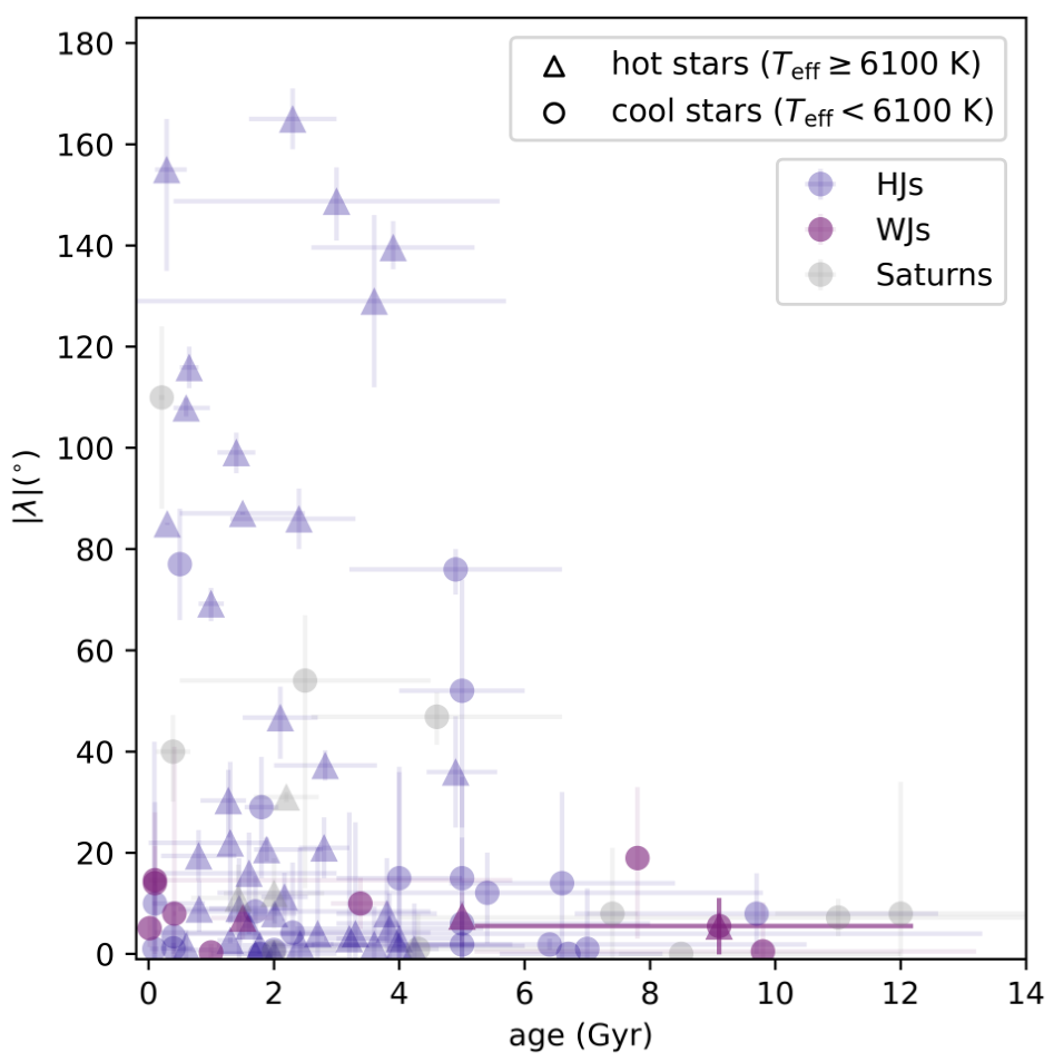
The ages in our sample were, like other parameters described in Section V.1, drawn from the NASA Exoplanet Archive and supplemented with values either directly from the literature or from the Extrasolar Values Encyclopaedia where possible. As shown in Figure 6, hot Jupiters in single-star systems are typically aligned at ages Gyr, while they are sometimes misaligned at Gyr. By contrast, all warm Jupiters in our sample are aligned irrespective of their age, including several systems with Gyr.
The age distribution of hot Jupiter misalignments, paired with the absence of this trend in tidally detached warm Jupiter systems, is consistent with the framework of tidal realignment. However, degeneracies between stellar and age complicate the interpretation of Figure 6. For example, cool stars are observed at a wider range of ages than hot stars due to their long main-sequence lifetimes – reflected by the near-absence of hot stars with Gyr in our sample. Hot stars also cool over time after they finish burning hydrogen in their cores, such that initially hot stars may be observed with K at later ages (Triaud 2011). Therefore, the apparent trend with age observed among the hot Jupiter population may instead be more telling of intrinsic differences between hot and cool star systems (Safsten et al. 2020).
To account for the heterogeneous stellar types within our sample, we next considered metrics for the tidal realignment timescale, characterized by the dimensionless tidal parameter . As shown in Figure 7, hot Jupiters – particularly those orbiting cool stars – can have relatively short tidal realignment timescales, whereas warm Jupiters and Saturn-mass planets have comparatively longer tidal realignment timescales.

In spite of their long tidal realignment timescales, warm Jupiters in single-star systems have not been found with large misalignments (). Importantly, the scale factor for the planetary realignment timescale is not well-constrained in the equilibrium tides framework considered here. However, the young ages of many warm Jupiter systems (six with estimated ages Gyr; see Figure 6), paired with the prevalence of aligned warm Jupiters with relatively large – despite the observation of some misaligned hot Jupiters with smaller values – suggests that these systems were likely not all realigned over their lifetimes. Several systems containing Saturn-mass planets have been found with substantial misalignments, suggesting that these planets, which have some of the longest tidal realignment timescales in our sample, may be more susceptible to misalignment via dynamical interactions with neighboring planets.
V.4 Caveats and Uncertainties
We emphasize that our sample is heterogeneous: the measurements within our population study are drawn from many individual studies. Certain measurements would be particularly helpful to verify with additional observations: for example, our results are largely driven by the small sample of misaligned systems that have been observed, but the Rossiter-McLaughlin measurements of two misaligned hot Jupiter measurements in cool star systems include little to no egress data (e.g. CoRoT-19 b (Guenther et al. 2012) and HATS-14 b (Zhou et al. 2015)), providing weaker constraints on the obliquity of each system. Furthermore, underestimated values can mimic a low-amplitude Rossiter-McLaughlin signal, which may be incorrectly interpreted as a polar orbit. Additional tests to verify and more precisely constrain the obliquities of misaligned systems will be crucial to confirm or to challenge the results presented in this work.
Our cutoff between “hot” and “warm” Jupiters at was selected empirically and is not necessarily the “true” cutoff between the two populations. A shifted cutoff of , which expands the sample of warm Jupiters by four systems (two with ), still reveals a tentative trend toward warm Jupiters being more aligned than hot Jupiters, with an adjusted significance of , , and for the left, center, and right panel of Figure 4, respectively. Different sets of stellar parameters may also shift individual systems slightly in space; for example, KELT-6 b is listed with in Albrecht et al. 2012.
A transition range may exist between the hot and warm Jupiter populations, with a rate of misalignments that is reduced relative to that of the close-in hot Jupiters but that is higher than that of the tidally detached warm Jupiters. Additional measurements for planets near will help to better sculpt the landscape of this parameter space and to potentially constrain the tidal realignment timescale for planets.
VI Discussion
VI.1 Implications for Hot and Warm Jupiter Evolution
We have demonstrated that, in single-star systems, the tidally detached warm Jupiter population is substantially more aligned than the hot Jupiter population, despite hot Jupiters’ bias toward potentially realigned systems. This result has two key implications: (1) planets in single-star systems typically form within aligned protoplanetary disks, and (2) warm Jupiters form quiescently, whereas hot Jupiters are likely misaligned after the protoplanetary disk has dispersed.
Quiescently formed warm Jupiters should remain roughly within the plane of their natal protoplanetary disk. As a result, if misalignments typically originate at the protoplanetary disk stage, then quiescently formed warm Jupiters should be observed with a similarly high rate of misalignments to that of the hot Jupiter population. In this scenario, observational biases should favor a higher rate of misaligned warm Jupiters, since these tidally detached systems are unable to realign over timescales within the age of the Universe.
By contrast, the population of tidally detached warm Jupiters is significantly more aligned than the population of close-orbiting hot Jupiters. We conclude that warm Jupiters in single-star systems typically form within disks that are aligned with the host star’s equator, whereas misalignments in hot Jupiter systems typically arise after the disk dispersal phase. This framework is consistent with the high rate of observed planetary companions in quiescent warm Jupiter systems (Huang et al. 2016), by contrast with a much lower companion rate in hot Jupiter systems (Steffen et al. 2012) that may have lost their companions during the misalignment process.
This framework is also supported by previous observations from the Atacama Large Millimeter Array (ALMA) that have suggested that most, if not all, protoplanetary disks are aligned with the spin axis of their host stars (Davies 2019). Furthermore, no misaligned planets have been found in very young systems with Myr (Albrecht et al. 2022). While the sample of planets in this parameter space is small (only 6 to date), the absence of misaligned planets in young systems is consistent with our framework in which misalignments originate later in the systems’ evolution.
Previous results have demonstrated that hot Jupiters’ observed misalignments are fully consistent with a dominant formation mechanism that is dynamically violent (Rice et al. 2022). Many hot Jupiters that are currently observed in aligned configurations may have been misaligned earlier in their evolution and subsequently realigned over time through star-planet tidal interactions. The closest-orbiting hot Jupiters around the coolest stars are typically all aligned, suggesting that tidal interactions have played an important role in the orbital evolution of these systems (Wang et al. 2021).
Some promising hot Jupiter misalignment mechanisms, such as the Kozai-Lidov mechanism in stellar binaries (Naoz et al. 2012), require the presence of a stellar companion. However, the high rate of hot Jupiter misalignments, even in single-star systems, indicates that hot Jupiters cannot be misaligned exclusively through interactions with a stellar companion.
Instead, planet-planet interactions likely play an important role in the production of hot Jupiters’ misalignments. Alternative mechanisms invoking one or more planetary companions include secular chaos in multiplanet systems with overlapping resonances (Wu & Lithwick 2011; Teyssandier et al. 2019) and planet-planet scattering (Rasio & Ford 1996), particularly when combined with the Kozai-Lidov mechanism (Naoz et al. 2011; Nagasawa & Ida 2011).
VI.2 The Evolution of Extrasolar Saturns
While examining the hot and warm Jupiter populations, we also found that Saturn-mass planets, including those at a wide orbital separation , span a wide range of spin-orbit angles. Three of the four misaligned Saturns in our sample (TOI-1268 b,66 6 Dong et al. 2022 includes 3 separate measurements for TOI-1268 b. While we adopt the value included in the TEPcat catalogue, we note that the other two provided measurements each indicate a lower sky-projected obliquity ( and , from two separate reductions of the same NEID dataset). As a result, this system may not be strongly misaligned. Kepler-63 b, and WASP-117 b) have significant projected eccentricities (), suggesting that their eccentricities and stellar obliquities may have been jointly elevated. Three processes that can produce eccentric, misaligned Saturns include the adiabatic disk-dispersal resonance proposed by Petrovich et al. 2020, Kozai-Lidov interactions (Naoz et al. 2011), and secular chaos (Wu & Lithwick 2011).
VI.2.1 Disk-Dispersal Resonance
The Petrovich et al. 2020 disk-dispersal resonance was originally proposed as a mechanism to naturally produce polar Neptunes—a growing population of observed systems (Stefansson et al. 2021; Albrecht et al. 2022). This resonance occurs when the nodal precession rate of an outer planetary companion, induced by interactions with the protoplanetary disk, reaches commensurability with the nodal precession rate of the inner planet, induced by general relativistic effects and the stellar quadrupole field.
The same mechanism can also extend to higher-mass planets, with the caveat that a larger initial mutual inclination is required between the inner planet and its outer companion to ensure conservation of the angular momentum deficit :
| (11) |
Here, and are the orbital angular momenta of the inner and outer planet, while and are the planets’ inclinations.
The mutual inclination required to conserve is given by
| (12) |
Here, and are the masses of the inner and outer planet, respectively, while and are the corresponding semimajor axes. For a Neptune-mass planet at au with a companion at au, the required mutual inclination is only . By contrast, if the inner planet is set to be Saturn-mass.
Therefore, the population of misaligned Saturns may represent the upper mass limit of inner planets to which this mechanism applies. This would also imply a limit to the typical values attained during disk dispersal, with a larger limit required for lower-mass outer companions.
VI.2.2 Kozai-Lidov
The Saturns in our sample may instead be misaligned by the Kozai-Lidov mechanism. In this framework, a third perturber with a significant initial mutual inclination () is required to initialize a secular exchange of eccentricity and inclination between hierarchical orbits (Naoz 2016). In single-star systems, this additional perturber could be a companion planet within the system. However, this raises the question of why Saturn-mass planets would be misaligned, while warm Jupiters would not.
If Saturns are misaligned through Kozai-Lidov oscillations, this would imply that Saturns more commonly appear in systems that meet the mechanism’s required initial conditions. Planet-planet scattering simulations have offered evidence that, in systems with equal-mass planets, lower-mass planets preferentially reach higher mutual inclinations from planet-planet scattering. For example, Raymond et al. 2010 found that 10% of unstable planets in their disk-free simulations reached inclinations larger than 39 in J-J-J systems (3 Jupiters), 42 in S-S-S systems (3 Saturns), and 49 in N-N-N systems (3 Neptunes). This increase in mutual inclinations with decreasing planet mass reflects the ease with which higher-mass planets can eject each other from the system, reducing the total number of close encounters over the systems’ evolution. Therefore, the misaligned Saturns within our sample may represent a mass cutoff below which scattering processes can produce mutual inclinations .
So far, no planetary companions have been found in any of the single-star Saturn systems that show evidence for misalignment. However, long-period Saturn-mass companions also cannot be ruled out based on current radial velocity surveys (e.g. Figure 1 in Fulton et al. 2021). If the relatively high occurrence rate of misaligned Saturn-mass planets emerges due to planet-planet scattering combined with the Kozai-Lidov mechanism, we anticipate that outer planetary companions should be prevalent in misaligned Saturn systems.
VI.2.3 Secular Chaos
Secular chaos may also play a role in misaligning the Saturns observed in our sample. Secular chaos requires the presence of at least planets in an individual system, and it is produced by overlapping, nonlinear secular resonances in which the precession rates of different planets reach commensurability (Lithwick & Wu 2011). Previous work has demonstrated that secular chaos can produce substantial spin-orbit misalignments in multiplanet systems (Wu & Lithwick 2011).
If Saturns form with neighboring companion planets, they may be misaligned through secular chaos in certain cases. However, spin-orbit angles larger than 90 are difficult to generate from secular chaos (Wu & Lithwick 2011; Teyssandier et al. 2019), such that highly misaligned systems (for example, Kepler-63, with (Sanchis-Ojeda et al. 2013)) likely could not have been misaligned by this mechanism. Furthermore, the secular chaos framework does not explain the heightened rate of spin-orbit misalignments for Saturn-mass planets as compared with warm Jupiters.
Because secular chaos takes place over timescales similar to or longer than the secular precession timescale, this framework would imply that misaligned Saturns should typically be observed at older stellar ages. Misaligned hot Jupiters have recently been found to be more common at older stellar ages (Hamer & Schlaufman 2022), providing evidence that secular chaos may be prevalent in at least some misaligned giant planet systems.
VII Conclusions
In this work, we have measured the Rossiter-McLaughlin effect across the transit of tidally detached warm Jupiter TOI-1478 b using the Keck/HIRES and WIYN/NEID instruments. This is the third measurement made as part of the SOLES survey, which is designed to constrain planetary evolution models by studying stellar obliquities in long-period exoplanet systems.
We combined this measurement with archival stellar obliquity constraints in single-star systems to conduct a population study demonstrating the statistical significance with which warm Jupiters are more aligned than analogous hot Jupiters. Our findings are summarized as follows:
- •
The TOI-1478 system is consistent with alignment, with sky-projected spin-orbit angle .
- •
The previous value for TOI-1478 may have been overestimated, as indicated by the low Rossiter-McLaughlin amplitude of the system.
- •
The current set of stellar obliquity constraints indicates that warm Jupiters in single-star systems are preferentially more aligned than analogous hot Jupiters (at when considering the full population, and at when comparing to hot stars that presumably have not experienced tidal realignment).
- •
Even when considering only systems around cool stars, warm Jupiters still appear to be more misaligned than analogous hot Jupiters (at ). However, further measurements are needed to better constrain the prevalence of misaligned hot Jupiters in cool, single-star systems and to verify the robustness of this result.
- •
Saturn-mass planets span a wide range of sky-projected spin-orbit angles, even at wide orbital separation.
Based on these findings, we conclude that (1) planets in single-star systems tend to form within aligned protoplanetary disks and (2) warm Jupiters tend to form quiescently, while hot Jupiters are misaligned after protoplanetary disk dispersal. We have also proposed several potential explanations for the preferential misalignment of Saturn-mass planets, including a secular disk-dispersal resonance, the Kozai-Lidov mechanism, or secular chaos.
Additional stellar obliquity measurements for warm Jupiters in binary star systems are needed to evaluate whether the observed trends extend beyond single-star systems. Further warm Jupiter spin-orbit angle measurements will also help to elucidate any potential correlations between eccentricities and stellar obliquities, which may provide improved insights into the key mechanisms contributing to extrasolar system misalignments.
VIII Acknowledgements
We thank our anonymous reviewer for their comments that have strengthened this manuscript. Over the duration of this project, M.R. was supported by the Heising-Simons Foundation 51 Pegasi b Fellowship and by the National Science Foundation Graduate Research Fellowship Program under Grant Number DGE-1752134. The data presented herein were obtained at the W. M. Keck Observatory, which is operated as a scientific partnership among the California Institute of Technology, the University of California and the National Aeronautics and Space Administration. The Observatory was made possible by the generous financial support of the W. M. Keck Foundation. This work is supported by the Astronomical Big Data Joint Research Center, co-founded by National Astronomical Observatories, Chinese Academy of Sciences and Alibaba Cloud. This research has made use of the Keck Observatory Archive (KOA), which is operated by the W. M. Keck Observatory and the NASA Exoplanet Science Institute (NExScI), under contract with the National Aeronautics and Space Administration. This research has made use of the NASA Exoplanet Archive, which is operated by the California Institute of Technology, under contract with the National Aeronautics and Space Administration under the Exoplanet Exploration Program. This paper contains data taken with the NEID instrument, which was funded by the NASA-NSF Exoplanet Observational Research (NN-EXPLORE) partnership and built by Pennsylvania State University. NEID is installed on the WIYN 3.5m telescope at KPNO, which is managed by the Association of Universities for Research in Astronomy (AURA) under a cooperative agreement with the NSF. The NEID archive is operated by the NASA Exoplanet Science Institute at the California Institute of Technology. We thank the NEID Queue Observers and WIYN Observing Associates for their skillful execution of our NEID observations. The authors are honored to be permitted to conduct astronomical research on Iolkam Du’ag (Kitt Peak), a mountain with particular significance to the Tohono O’odham.
Keck: I (HIRES), WIYN (NEID), Exoplanet Archive, Extrasolar Planets Encyclopaedia
References
- Albrecht et al. (2012) Albrecht, S., Winn, J. N., Johnson, J. A., et al. 2012, The Astrophysical Journal, 757, 18
- Albrecht et al. (2022) Albrecht, S. H., Dawson, R. I., & Winn, J. N. 2022, arXiv preprint arXiv:2203.05460
- Albrecht et al. (2021) Albrecht, S. H., Marcussen, M. L., Winn, J. N., Dawson, R. I., & Knudstrup, E. 2021, The Astrophysical Journal Letters, 916, L1
- Blanco-Cuaresma (2019) Blanco-Cuaresma, S. 2019, Monthly Notices of the Royal Astronomical Society, 486, 2075
- Blanco-Cuaresma et al. (2014) Blanco-Cuaresma, S., Soubiran, C., Heiter, U., & Jofré, P. 2014, Astronomy & Astrophysics, 569, A111
- Bourrier et al. (2017) Bourrier, V., Cegla, H., Lovis, C., & Wyttenbach, A. 2017, Astronomy & Astrophysics, 599, A33
- Brewer et al. (2016) Brewer, J. M., Fischer, D. A., Valenti, J. A., & Piskunov, N. 2016, The Astrophysical Journal Supplement Series, 225, 32
- Brown et al. (2021) Brown, A. G., Vallenari, A., Prusti, T., et al. 2021, Astronomy & Astrophysics, 649, A1
- da Silva et al. (2006) da Silva, L., Girardi, L., Pasquini, L., et al. 2006, A&A, 458, 609
- Davies (2019) Davies, C. L. 2019, Monthly Notices of the Royal Astronomical Society, 484, 1926
- Dong et al. (2022) Dong, J., Huang, C. X., Zhou, G., et al. 2022, The Astrophysical Journal Letters, 926, L7
- El-Badry et al. (2021) El-Badry, K., Rix, H.-W., & Heintz, T. M. 2021, Monthly Notices of the Royal Astronomical Society, 506, 2269
- Fűrész (2008) Fűrész, G. 2008, PhD thesis, Univ. of Szeged, Hungary
- Fontanive & Bardalez Gagliuffi (2021) Fontanive, C., & Bardalez Gagliuffi, D. 2021, Frontiers in Astronomy and Space Sciences, 16
- Foreman-Mackey et al. (2013) Foreman-Mackey, D., Hogg, D. W., Lang, D., & Goodman, J. 2013, PASP, 125, 306
- Fulton et al. (2021) Fulton, B. J., Rosenthal, L. J., Hirsch, L. A., et al. 2021, The Astrophysical Journal Supplement Series, 255, 14
- Gaia Collaboration et al. (2016) Gaia Collaboration, Prusti, T., de Bruijne, J. H. J., et al. 2016, A&A, 595, A1
- Gaia Collaboration et al. (2018) Gaia Collaboration, Brown, A., Vallenari, A., et al. 2018, arXiv preprint arXiv:1804.09365
- Gaidos et al. (2022) Gaidos, E., Hirano, T., Beichman, C., et al. 2022, Monthly Notices of the Royal Astronomical Society, 509, 2969
- Gray & Corbally (1994) Gray, R. O., & Corbally, C. J. 1994, 107, 742, tex.adsnote: Provided by the SAO/NASA Astrophysics Data System tex.adsurl: https://ui.adsabs.harvard.edu/abs/1994AJ….107..742G
- Grevesse et al. (2007) Grevesse, N., Asplund, M., & Sauval, A. J. 2007, Space Sci. Rev., 130, 105
- Guenther et al. (2012) Guenther, E., Díaz, R., Gazzano, J.-C., et al. 2012, Astronomy & Astrophysics, 537, A136
- Günther & Daylan (2020) Günther, M. N., & Daylan, T. 2020, arXiv preprint arXiv:2003.14371
- Hamer & Schlaufman (2022) Hamer, J. H., & Schlaufman, K. C. 2022, arXiv preprint arXiv:2205.00040
- Harris et al. (2020) Harris, C. R., Millman, K. J., van der Walt, S. J., et al. 2020, Nature, 585, 357
- Heiter et al. (2015) Heiter, U., Lind, K., Asplund, M., et al. 2015, Phys. Scr, 90, 054010
- Hjorth et al. (2021) Hjorth, M., Albrecht, S., Hirano, T., et al. 2021, Proceedings of the National Academy of Sciences, 118, e2017418118
- Howard et al. (2010) Howard, A. W., Johnson, J. A., Marcy, G. W., et al. 2010, The Astrophysical Journal, 721, 1467
- Huang et al. (2016) Huang, C., Wu, Y., & Triaud, A. H. 2016, The Astrophysical Journal, 825, 98
- Hunter (2007) Hunter, J. D. 2007, Computing in science & engineering, 9, 90
- Johnson et al. (2022) Johnson, M. C., David, T. J., Petigura, E. A., et al. 2022, The Astronomical Journal, 163, 247
- Kaufer et al. (1999) Kaufer, A., Stahl, O., Tubbesing, S., et al. 1999, The Messenger, 95, 8
- Kesseli et al. (2018) Kesseli, A. Y., Muirhead, P. S., Mann, A. W., & Mace, G. 2018, The Astronomical Journal, 155, 225
- Kraft (1967) Kraft, R. P. 1967, The Astrophysical Journal, 150, 551
- Lithwick & Wu (2011) Lithwick, Y., & Wu, Y. 2011, The Astrophysical Journal, 739, 31
- Mancini et al. (2015) Mancini, L., Esposito, M., Covino, E., et al. 2015, Astronomy & Astrophysics, 579, A136
- Markwardt (2009) Markwardt, C. B. 2009, in Astronomical Society of the Pacific Conference Series, Vol. 411, Astronomical Data Analysis Software and Systems XVIII, ed. D. A. Bohlender, D. Durand, & P. Dowler, 251
- McKinney et al. (2010) McKinney, W., et al. 2010, in Proceedings of the 9th Python in Science Conference, Vol. 445, Austin, TX, 51–56
- McLaughlin (1924) McLaughlin, D. 1924, The Astrophysical Journal, 60
- Nagasawa & Ida (2011) Nagasawa, M., & Ida, S. 2011, The Astrophysical Journal, 742, 72
- Naoz (2016) Naoz, S. 2016, Annual Review of Astronomy and Astrophysics, 54, 441
- Naoz et al. (2011) Naoz, S., Farr, W. M., Lithwick, Y., Rasio, F. A., & Teyssandier, J. 2011, Nature, 473, 187
- Naoz et al. (2012) Naoz, S., Farr, W. M., & Rasio, F. A. 2012, The Astrophysical Journal Letters, 754, L36
- NASA Exoplanet Archive (2022) NASA Exoplanet Archive. 2022, Planetary Systems, vVersion: 2022-02-19 12:08, NExScI-Caltech/IPAC, doi:10.26133/NEA12. https://catcopy.ipac.caltech.edu/dois/doi.php?id=10.26133/NEA12
- Ness et al. (2015) Ness, M., Hogg, D. W., Rix, H.-W., Ho, A. Y., & Zasowski, G. 2015, The Astrophysical Journal, 808, 16
- Nofi et al. (2021) Nofi, L. A., Johns-Krull, C. M., López-Valdivia, R., et al. 2021, The Astrophysical Journal, 911, 138
- Oliphant (2006) Oliphant, T. E. 2006, A guide to NumPy, Vol. 1 (Trelgol Publishing USA)
- Park et al. (2014) Park, C., Jaffe, D. T., Yuk, I.-S., et al. 2014, in Ground-based and Airborne Instrumentation for Astronomy V, Vol. 9147, SPIE, 510–521
- Paxton et al. (2010) Paxton, B., Bildsten, L., Dotter, A., et al. 2010, The Astrophysical Journal Supplement Series, 192, 3
- Paxton et al. (2013) Paxton, B., Cantiello, M., Arras, P., et al. 2013, The Astrophysical Journal Supplement Series, 208, 4
- Paxton et al. (2015) Paxton, B., Marchant, P., Schwab, J., et al. 2015, The Astrophysical Journal Supplement Series, 220, 15
- Pepper et al. (2012) Pepper, J., Kuhn, R. B., Siverd, R., James, D., & Stassun, K. 2012, Publications of the Astronomical Society of the Pacific, 124, 230
- Pepper et al. (2018) Pepper, J., Stassun, K. G., & Gaudi, B. S. 2018, Handbook of Exoplanets, 1
- Pepper et al. (2007) Pepper, J., Pogge, R. W., DePoy, D., et al. 2007, Publications of the Astronomical Society of the Pacific, 119, 923
- Petrovich et al. (2020) Petrovich, C., Muñoz, D. J., Kratter, K. M., & Malhotra, R. 2020, The Astrophysical Journal Letters, 902, L5
- Pollacco et al. (2006) Pollacco, D. L., Skillen, I., Cameron, A. C., et al. 2006, Publications of the Astronomical Society of the Pacific, 118, 1407
- Queloz et al. (2001) Queloz, D., Mayor, M., Udry, S., et al. 2001, The Messenger, 105, 1
- Queloz et al. (2010) Queloz, D., Anderson, D., Cameron, A. C., et al. 2010, Astronomy & Astrophysics, 517, L1
- Rasio & Ford (1996) Rasio, F. A., & Ford, E. B. 1996, Science, 274, 954
- Raymond et al. (2010) Raymond, S. N., Armitage, P. J., & Gorelick, N. 2010, The Astrophysical Journal, 711, 772
- Rice & Brewer (2020) Rice, M., & Brewer, J. M. 2020, The Astrophysical Journal, 898, 119
- Rice et al. (2022) Rice, M., Wang, S., & Laughlin, G. 2022, The Astrophysical Journal Letters, 926, L17
- Rice et al. (2021) Rice, M., Wang, S., Howard, A. W., et al. 2021, The Astronomical Journal, 162, 182
- Ricker et al. (2015) Ricker, G. R., Winn, J. N., Vanderspek, R., et al. 2015, Journal of Astronomical Telescopes, Instruments, and Systems, 1, 014003
- Rodriguez et al. (2021) Rodriguez, J. E., Quinn, S. N., Zhou, G., et al. 2021, The Astronomical Journal, 161, 194
- Rogers et al. (2012) Rogers, T., Lin, D. N., & Lau, H. H. B. 2012, The Astrophysical Journal Letters, 758, L6
- Rossiter (1924) Rossiter, R. 1924, The Astrophysical Journal, 60
- Safsten et al. (2020) Safsten, E. D., Dawson, R. I., & Wolfgang, A. 2020, The Astronomical Journal, 160, 214
- Sanchis-Ojeda et al. (2013) Sanchis-Ojeda, R., Winn, J. N., Marcy, G. W., et al. 2013, The Astrophysical Journal, 775, 54
- Santerne et al. (2014) Santerne, A., Hébrard, G., Deleuil, M., et al. 2014, Astronomy & Astrophysics, 571, A37
- Schwab et al. (2016) Schwab, C., Rakich, A., Gong, Q., et al. 2016, in Ground-based and Airborne Instrumentation for Astronomy VI, Vol. 9908, International Society for Optics and Photonics, 99087H
- Schwarz et al. (2016) Schwarz, R., Funk, B., Zechner, R., & Bazsó, Á. 2016, Monthly Notices of the Royal Astronomical Society, 460, 3598
- Southworth (2011) Southworth, J. 2011, Monthly Notices of the Royal Astronomical Society, 417, 2166
- Stassun & Torres (2018) Stassun, K. G., & Torres, G. 2018, ApJ, 862, 61
- Stefansson et al. (2021) Stefansson, G., Mahadevan, S., Petrovich, C., et al. 2021, arXiv preprint arXiv:2111.01295
- Steffen et al. (2012) Steffen, J. H., Ragozzine, D., Fabrycky, D. C., et al. 2012, Proceedings of the National Academy of Sciences, 109, 7982
- Teyssandier et al. (2019) Teyssandier, J., Lai, D., & Vick, M. 2019, Monthly Notices of the Royal Astronomical Society, 486, 2265
- Tokovinin et al. (2013) Tokovinin, A., Fischer, D. A., Bonati, M., et al. 2013, PASP, 125, 1336
- Triaud (2011) Triaud, A. H. 2011, Astronomy & Astrophysics, 534, L6
- Triaud (2017) —. 2017, arXiv preprint arXiv:1709.06376
- Valenti & Fischer (2005) Valenti, J. A., & Fischer, D. A. 2005, The Astrophysical Journal Supplement Series, 159, 141
- Virtanen et al. (2020) Virtanen, P., Gommers, R., Oliphant, T. E., et al. 2020, Nature methods, 17, 261
- Vogt et al. (1994) Vogt, S. S., Allen, S. L., Bigelow, B. C., et al. 1994, in Instrumentation in Astronomy VIII, Vol. 2198, International Society for Optics and Photonics, 362–375
- Wallace et al. (2011) Wallace, L., Hinkle, K., Livingston, W., & Davis, S. 2011, The Astrophysical Journal Supplement Series, 195, 6
- Walt et al. (2011) Walt, S. v. d., Colbert, S. C., & Varoquaux, G. 2011, Computing in Science & Engineering, 13, 22
- Wang et al. (2021) Wang, S., Winn, J. N., Addison, B. C., et al. 2021, The Astronomical Journal, 162, 50
- Wang et al. (2022) Wang, X.-Y., Rice, M., Wang, S., et al. 2022, The Astrophysical Journal Letters, 926, L8
- Wenger et al. (2000) Wenger, M., Ochsenbein, F., Egret, D., et al. 2000, Astronomy and Astrophysics Supplement Series, 143, 9
- Wu & Lithwick (2011) Wu, Y., & Lithwick, Y. 2011, The Astrophysical Journal, 735, 109
- Xu et al. (2019) Xu, X., Cisewski-Kehe, J., Davis, A. B., Fischer, D. A., & Brewer, J. M. 2019, The Astronomical Journal, 157, 243
- Zhou et al. (2015) Zhou, G., Bayliss, D., Hartman, J. D., et al. 2015, The Astrophysical Journal Letters, 814, L16
- Zhou et al. (2018) Zhou, G., Rodriguez, J. E., Vanderburg, A., et al. 2018, The Astronomical Journal, 156, 93
| System | Planet | () | Age (Gyr) | (K) | ||||
|---|---|---|---|---|---|---|---|---|
| Warm Jupiters: | ||||||||
| WASP-80 | b | |||||||
| WASP-53 | b | - | ||||||
| WASP-84 | b | |||||||
| HAT-P-17 | b | 7.8 | ||||||
| TOI-1478 | b | |||||||
| HD 63433 | b | |||||||
| K2-140 | b | |||||||
| HIP 67522 | b | |||||||
| WASP-25 | b | |||||||
| HD 17156 | b | |||||||
| WASP-38 | b | |||||||
| KOI-12 | b | |||||||
| Hot Jupiters: | ||||||||
| WASP-43 | b | |||||||
| Qatar-2 | b | |||||||
| Qatar-1 | b | |||||||
| TOI-942 | b | |||||||
| WASP-52 | b | |||||||
| HATS-2 | b | |||||||
| HATS-14 | b | |||||||
| CoRoT-18 | b | |||||||
| WASP-19 | b | |||||||
| WASP-4 | b | |||||||
| WASP-41 | b | |||||||
| WASP-47 | b | |||||||
| HAT-P-36 | b | |||||||
| WASP-16 | b | |||||||
| HAT-P-13 | b | |||||||
| WASP-5 | b | |||||||
| Kepler-17 | b | |||||||
| HAT-P-23 | b | |||||||
| CoRoT-1 | b | |||||||
| WASP-74 | b | |||||||
| WASP-28 | b | |||||||
| CoRoT-19 | b | |||||||
| WASP-32 | b | |||||||
| WASP-60 | b | |||||||
| WASP-103 | b | |||||||
| HD 209458 | b | |||||||
| K2-34 | b | |||||||
| WASP-22 | b | |||||||
| WASP-71 | b | |||||||
| Kepler-8 | b | |||||||
| WASP-62 | b | |||||||
| KELT-6 | b | |||||||
| WASP-61 | b | |||||||
| HAT-P-2 | b | |||||||
| CoRoT-11 | b | |||||||
| HAT-P-9 | b | |||||||
| HATS-3 | b | |||||||
| XO-4 | b | |||||||
| WASP-190 | b | |||||||
| XO-3 | b | |||||||
| HAT-P-34 | b | |||||||
| WASP-87 | b | |||||||
| NGTS-2 | b | |||||||
| WASP-7 | b | |||||||
| TOI-2109 | b | |||||||
| WASP-17 | b | |||||||
| HAT-P-56 | b | |||||||
| HAT-P-6 | b | |||||||
| WASP-15 | b | |||||||
| WASP-121 | b | |||||||
| WASP-79 | b | |||||||
| WASP-66 | b | |||||||
| XO-6 | b | |||||||
| KELT-7 | b | |||||||
| WASP-100 | b | - | ||||||
| TOI-1518 | b | - | ||||||
| KELT-17 | b | - | ||||||
| MASCARA-1 | b | |||||||
| KELT-21 | b | |||||||
| TOI-1431 | b | |||||||
| HAT-P-69 | b | |||||||
| HATS-70 | b | |||||||
| HAT-P-70 | b | |||||||
| KELT-20 | b | - | ||||||
| KELT-9 | b | |||||||
| Saturns: | ||||||||
| HAT-P-12 | b | 0 | ||||||
| WASP-69 | b | 0 | ||||||
| TOI-1268 | b | |||||||
| WASP-6 | b | |||||||
| WASP-148 | b | - | ||||||
| WASP-39 | b | 0 | ||||||
| Kepler-63 | b | 0.45 | ||||||
| WASP-21 | b | 0 | ||||||
| WASP-13 | b | 0 | ||||||
| WASP-117 | b | |||||||
| HD 332231 | b | |||||||
| HD 149026 | b | 0 | ||||||
| K2-232 | b | |||||||
| WASP-174 | b | 0 |