Image warp preserving content intensity
Abstract
An accurate method for warping images is presented. Differently from most commonly used techniques, this method guarantees the conservation of the intensity of the transformed image, evaluated as the sum of its pixel values over the whole image or over corresponding transformed subregions of it. Such property is mandatory for quantitative analysis, as, for instance, when deformed images are used to assess radiances, to measure optical fluxes from light sources, or to characterize material optical densities. The proposed method enforces area resampling by decomposing each rectangular pixel in two triangles, and projecting the pixel intensity onto half pixels of the transformed image, with weights proportional to the area of overlap of the triangular half-pixels. The result is quantitatively exact, as long as the original pixel value is assumed to represent a constant image density within the pixel area, and as long as the coordinate transformation is diffeomorphic. Implementation details and possible variations of the method are discussed.
keywords
Warping, Area resampling, Image distortion, PhotometryAMS
68U10, 65D18, 54H301 Introduction
Many scientific procedures which make quantitative use of the image content, in fields which range from microscopy to astronomy, require images to be transformed and remapped onto deformed coordinates system. Typical applications include the correction of geometrical aberrations produced by imaging systems, the mutual registration of scenes recorded with different optical systems or from different points of view [44, 23]; stitching together different images with partial overlap among themselves [13], also referred to as multi-frame joint image registration; the fusion and proper coadding of different images of the same source fields [42]. In medical imaging and computational anatomy in particular, to name another application, cross image registration is always required to properly compare features of compliant soft tissue. Furthermore, dynamic mapping of image sequences over deforming templates was used with expressive intent in yesteryears, in a procedure called “morphing” [38, 27] where the appearance of one object was transformed smoothly into that of another (e.g. a human figure into an animal) by means of gradual deformation and blending.
For our purposes, we consider two dimensional images, generically represented as two dimensional arrays of values of the intensity over Cartesian grids. The methods for determining the appropriate geometrical transformation between the source and the target coordinates are varied and sophisticated [14, 24], depend on the task, and are not themselves of concern of this paper. Such methods may make use of functional relations between the coordinate systems known a priori, or may rely on the identification of common landmark features appearing in the images [3, 20], either known from supervised annotation, from model fit or from trained deep learning (e.g. [41, 43]). In computational anatomy, for instance, diffeomorphic flow is assumed between source and target images, and LDDMM [2] in a number of variants is very popular. A large body of literature exists on these methods, which do not need to be reviewed here. Once the functional transformation which maps the two systems of coordinates is established, a “best” way of transforming also the image values is sought. The acception of “best” is sometimes subjective and in many cases depends on the application: it may refer to a cosmetically pleasing result, to an optimal way of representing and preserving sharp level transitions in the destination image, or to the suppression of moiré or aliasing artifacts. Optimal ways of prefiltering and resampling of transformed images by means of interpolation are well described in literature [26, 1, 12] and implemented in widely adopted software libraries (e.g. OpenCV [4], scikit [35], ImageMagick [18]) as well as in graphic applications. In other cases, like in superresolution imaging and reconstruction [22], the recovery of realistic, underresolved image details is achieved relying on a priori subscale models, or optimal use of information resulting from multiple low resolution images belonging to a sequence. In this paper, in contrast, we describe a procedure which is purely intended to preserve the brightness of the image content across the transformation, even when the images are not Nyquist sampled, without invoking any help from the image data itself or from a priori knowledge of structure lost by the process of image formation. In simple terms, we exactly redistribute the whole intensity content of the source pixels over the target raster. The procedure is linear, and amounts to the determination of a reweighting matrix which projects the pixel values from the source to the destination image, and most importantly, depends only on the coordinate transform and not on the image data itself. As such, some variants of the procedure can be devised from the basic scheme, including one which provides a stable alternative to image interpolation without ad hoc filtering.
Our procedure implements a rigorous area resampling. The concept is known even from earlier literature, but does not seem to have received adequate attention, probably because of its higher computational cost which hinders its applications, and does not seem to have been pursued in the general case. Early attempts include that of [9], which proposes a fast implementation, based on a scanline decomposition. Scanline approaches treat the deformation of a raster image by carrying on some of the intensity content from one pixel to its adjacent in scan order, and are not proven to be exact for transformations beyond simple shears. A simpler version of Fant’s algorithm, applied only to raster resizing, goes under the name of pixel mixing [31] and was probably implemented in the open first by the pamscale function of the netpbm package [28]. The thesis [5] generalizes the problem, introducing the term “imaging-consistent integrating resampler”, taking into account also the point spread function of the imager, and blurring in image formation. The algorithm proposed there, though, still falls within the category of separable, scanline approaches, with a single accumulation register providing intensity remainders carried over from one pixel to the next. Another double pass, scanline algorithm is that of [16]. The seminal thesis [17] discusses the problem, and gives a partial solution in terms of adaptive local deformation of circular neighborhoods. This method is also implemented in the popular software package ImageMagick [33]. Another cognate approach proposed, and employed specifically for oversampling stacks of dithered astronomical images while preserving photometry, is “Drizzle” [11], but it relies on empirical factors, and treats both source and destination pixels as squares. “Drizzling” estimates pixel area overlaps using a sort of a Montecarlo approach, where the randomness is provided by inter-image pixel shifts. As a procedure, it some offers other advantages like the possibility of assigning individual quality weights to each contributing pixel; still it is not general for arbitrary deformations.
In summary, the existing literature on area resampling concentrated on the search for “efficient” variants of the method, or which seem to lack generality or exactness, when specifically looking at the preservation of the photometric intensity. It is our intention to discuss here a rigorous procedure, and its implementation.
The paper is organized as follows: section section 2 describes the geometrical principle of pixel remapping, section section 3 outlines the algorithm used, section section 4 demonstrates it, section section 5 discusses some variations, section section 6 shows the advantage of area resampling in photometric measurements, and section section 7 concludes and outlines future perspectives. Computational details are included in the appendices: the convention adopted for barycentric coordinates is given in appendix appendix A; appendix appendix B discusses the problem of intersecting triangles, and code performance is reported in appendix appendix C.
2 Exact area resampling by pixel triangulation
We start from an intensity image, given as a set of pixel values , representing the cumulative value of some quantity (for instance, the number of photons impinging the area of an individual photosensitive element), integrated over the rectangular pixel , defined as the rectangle , , for and . For simplicity we will treat here an equispaced coordinate grid, and , though the procedure can be easily generalized to non-equispaced plaid grids. We consider an a priori given bijective and differentiable coordinate transformation . We assume that the underlying intensity density inside the pixel is uniform, and that . Therefore, , where is the area of the pixel.
Our goal is to produce a new image of pixels, transforming the set of values into a new set on a new equispaced grid , with , and spacing , , in such a way that the cumulative intensity within any closed contour is preserved by the transformation:
| (1) |
for any region , and assuming an underlying transformed intensity density in the destination image. A natural way of achieving this property is to consider the quadrilateral , which approximates (to second order in , ) the transform of the rectangular pixel , identified by the set of its four vertices (see Fig. fig. 1). Save for singular or extreme deformations and coarse griddings which are of little practical interest, we can tacitly assume that remains a convex quadrilateral (concavity would imply a change of sign of the Jacobian of the transformation, violating the assumption of diffeomorphic transformation). For shorthand, we write , applying to polygons and contours as well as to individual points. Locally, this scalar density would be transformed as
| (2) |
so that, to second order, (eq. 1) is satisfied for and hence for any region composed of sets of pixels of image 1. Within the same approximation, we assume that the Jacobian is constant within and the density constant within . This position allows us to reduce the change of integration variable in Eq. (eq. 1) into a problem of decomposition of pixel areas: each fraction of projected on the destination grid, will contribute to the target intensity proportionally to its fractional area only.

The idea of considering the shape change of the pixel in the transformation is not new (see for example of the procedure described in §15.5 of [36]); however, our development is different in that we do not invoke arbitrary interpolations for the reconstruction of the destination image. The intensity of the rectangular pixel
on the target image is expressed as a sum of contributions
| (3) |
from each of the transformed pixels of image 1 partially overlapping with in image 2. The subset of indices to be taken into account is indicated here generically as “overlaps”; a criterion for selecting them will be formulated in the following. In (eq. 3), indicates the area of the resulting polygon. The procedure involves therefore two steps: 1) for any given destination pixel identify the set of original pixels whose transform overlaps with it, and 2) determine the polygonal shape of each intersection and compute its area.
The intersection of two convex quadrangles can be, in general, a polygon with anything between three and eight sides. Algorithms for the intersection of generic polygons exist in reputable computer geometry packages (e.g. in CGAL [10]), but their generality comes as a hindrance for our specialized case, requiring peculiar organized data structures, and is not necessarily optimal for a fast calculation. We prefer to simplify the task one step further. We divide both the origin pixel and the destination pixel in two triangles, splitting the quadrangles arbitrarily along one of their two diagonals, for instance and , and analogously and (Fig. fig. 2).

The task of identifying intersections between origin and destination pixels, required by Eq. (eq. 3), is split in that of finding the intersections between four times as many triangular half pixels. This is still non trivial, as there are no less than 17 possible, topologically different ways of intersecting two triangles (Figure fig. 9), excluding degenerate cases, as further discussed in appendix appendix B, but is definitely a simpler task than for quadrangles.
The same partial intensity is assigned to each of the two original triangles. Eq. (eq. 3) therefore expands into
| (4) |
Formally, the transformation between pixel intensities from the one to the other image can be written as
| (5) |
where is the incidence matrix detailing which fraction of intersects with . In typical cases, in which pixels of the original and of the destination rasters are of comparable sizes, this matrix is very sparse.
For transformations in which a source pixel is completely mapped on pixels on the the destination raster, the property holds. Conversely, gives a discretized representation of on the destination raster.
As an aside, once the transformation from to has been computed according to Eq. (eq. 5), its inverse can be obtained directly inverting the sparse matrix , for which numerical techniques are well studied. This may be more advantageous than using the inverse coordinate mapping, if using an algorithm like the one described in the next section, which exploits the fact that the source image grid is cartesian.
3 Algorithm layout
As resulting from (eq. 5), the intensity transformation between the two rasters reduces to a simple matrix multiplication, once the matrix elements are computed. To this extent, the steps sketched in inset algorithm 1 are required.
For each pixel of the source image, i.e. iterating on and :
- 1.
the coordinates of the vertices of each original hemipixel , are transformed with
- 2.
the set of hemipixels which have a non empty overlap with is determined
- 3.
the area of the intersections between each of the triangles of this set and each in turn, is found.
- 4.
the areas and are computed.
- 5.
the relevant contributions are summed to construct the matrix ,
Finally, the image is obtained by (eq. 5).
Step item 1 is the simple evaluation of a given function of the coordinates, and does not need to be described here. In the terminology of image processing, we are using naturally here a forward mapping between source and destination image.
For step item 2, all triangles which have at
least one vertex within the bounding box
are selected ( denoting the Cartesian product of the two
intervals). Since the triangular half pixels are defined on a
structured grid, they can be indexed in such a way that the criterion
is translated to a simple choice of indices, involving integer arithmetics.
It is algorithmically simpler to use this simplified criterion, which
may sometimes include additional disjoint triangles, than to refine
the search to the subset of triangles which have an actual intersection.
The condition for a positive overlap is not as simple as for instance
the requirement that vertices of fall internally to
or viceversa (figure fig. 9 provides
many counter examples).
The computation of overlap areas is more involved, and performed at step item 3. For that, we make due use of barycentric coordinates [6, 8] to reference the position of a point within a given triangle . In barycentric coordinates, the position of any point in the plane is determined by a triple of real numbers . This system has several properties that come to advantage for topological tests. With proper normalization, can be said to be internal to if all the three numbers are positive; falls on a side of if one of the three is null, and coincides with a vertex of if two are simultaneously null. Intersection points between two segments (in our case, sides of and of ) are easily computed from the barycentric coordinates of their extremes (equation eq. 18). Since a segment and the side of a triangle intersect only if the relevant barycentric coordinate of the extremes have opposite signs, inspection of the signs can also be used as a flag to avoid unnecessary computation of non existing crossings. Details are in Appendix appendix A.
Two possible algorithms for computing the areas of the triangle intersections needed for step item 3 are described in detail in Appendix appendix B. In our approach we make use of the one described in section B.4, which, albeit possibly slightly less efficient, is of much simpler implementation.
4 Warping examples and evaluation
We provide an example of the area resampling method using an 8 bit monochrome, pixels test image (boat.512, from [37]). The image coordinates are defined so that and ( increasing downwards). For the sake of illustration we take, as warping transformation,
| (6) |
which induces no deformation on the sides of the unit square, and has Jacobian comprised between . To quantify the numerical error in the preservation of intensity of the warped image, we compute the total intensity discrepance
| (7) |
The result of warping is shown in Figure fig. 3. The warp has been computed at various completely arbitrary resolutions, under and oversampling the image, to show the generality of the procedure. The calculation is performed in double precision floating point. The resulting , reported over each warped image, are barely over numerical precision.


5 Extensions
Alternative forms of the matrix element can be devised, giving different weights to the deformed pixel overlaps. The form of (eq. 4) distributes the available intensity separately on each destination hemipixel. Its effect can be appreciated in figure (fig. 4) for high downsampling ratio and non-affine pixel deformations, for which is significantly different from . Two other choices are presented in the following.


5.1 Pixel uniformity
Grouping together the two hemipixels, we can recast the total intensity of the original rectangular pixel onto the destination pixel, as actually prescribed by Eq. (eq. 3):
| (8) |
In other words, the contributions of the transformed half pixels and are weighted with a cumulative factor, which is the average of the two denominators in (eq. 4). The effect of this choice is illustrated in Fig. fig. 4. It may be argued that this weighting is more natural, as it preserves the original quadrangular pixel identity, rather than splitting it arbitrarily along one of its two diagonals.
5.2 Weighted area interpolation
In the intensity-preserving resampling illustrated before, we assign a contribution of pixel to the destination pixel which is proportional to to the inverse area of , i.e. we take into account the local stretch or contraction caused by the warp. If instead we weight the contribution according to the destination area covered, normalizing over the area of the destination pixel, as in
| (9) |
we achieve a form of area averaging and resampling. For a Cartesian grid, obviously . When undersampling, i.e. when several transformed pixels fall into a single destination pixel, their intensity values are averaged with a weight proportional to the area which they occupy on the destination; when oversampling, i.e. as a single deformed pixel covers more than a destination pixel, that destination pixel is assigned the same intensity of the source. This form can be thus seen as a value preserving warping, rather than an intensity preserving warping, and can be compared to other interpolation techniques in use in image processing.
5.2.1 Comparison with resampling interpolation
Figure fig. 5 provides a visual comparison of the merits of the weighted area interpolation based on Eq. (eq. 9) versus the commonly used bilinear interpolation, as a reference. Other more sophisticated interpolators, like higher order polynomial (e.g. bicubic, spline), Lanczos, or edge preserving (Akima), etc. could be compared as well, without affecting the main result. While many more interpolation methods are known in literature, the comparison with the simplest baseline algorithm is justified by the fact that the present area resampling recipe is only dependent on the geometry of the coordinate transform, not on the image data itself, nor on any assumed or a priori knowledge about the structure of the image. Other data-dependent interpolators (e.g. Takeda’s kernel regression [32], not to mention even more elaborate techniques based on deep learning) may produce more “realistic” results on the perceptual point of view, or even behave well as image denoisers (which implies a discrimination between an underlying image model and the superimposed corrupting noise). Here we merely report about the own merits of the weighted area resampler, without claiming that it is outperforming other image reconstruction techniques.
As an example of warping, we use the perspective transformation
| (10) |
which describes the projection of an image on the plane on the vertical plane , , , from the viewpoint , , .
To compare the two, we apply (eq. 5) and (eq. 9) using areas of triangles transformed from the to the space, i.e. using a direct coordinate transform. For the interpolation instead, we exploit a more efficient, customary implementation which evaluates the image values on the regular destination grid by looking up and interpolating values on . In other words, we perform an inverse pixel lookup. The transformation (eq. 10) has analytical inverse
| (11) |
with , , , , and for . To stress the essential differences between the two methods, no dealiasing filter prior to interpolation is applied.


Area resampling somehow averages many original image values falling on the destination pixels, whereas the traditional resampling only picks up one value or averages few neighbors, sampling those which fall close to an interpolation point. Area resampling provides thus a smoother result than interpolation when undersampling images, and can be less prone to aliasing, since in that case it automatically behaves as an adaptive box filter. Interpolation is affected by aliasing, which is usually cured by low pass prefiltering; however, for a general warp transformation this filtering has to be local [17], complicating matters. An example of aliasing reduction is shown in Figure fig. 6, where a global rescaling ratio and a simple periodic pattern evidence the different amplitude of the aliased spatial component. The amount of alias suppression, though, is entirely dependent on the particular local downsampling ratio, and on the original image content.
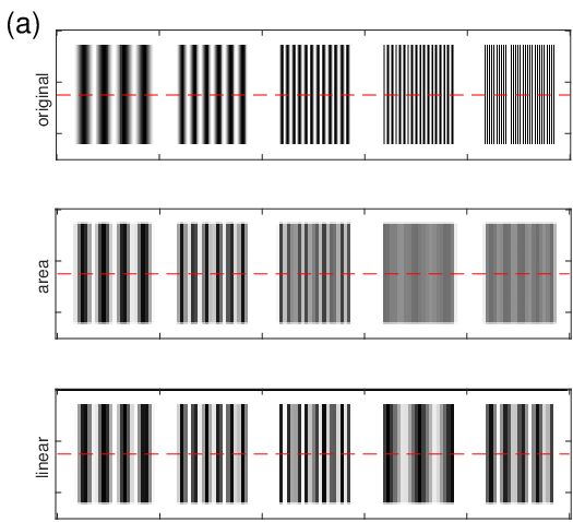

On the other hand, when oversampling, the weighted area transform produces images which are sharper and more faithful to pixel edges, since the destination value picked in that case represents well the original pixel value, rather than being an interpolation between nearest neighbors.
6 Example: source photometry
Preservation of the intensity is an essential property when photometry is performed on deformable images. We show in figure fig. 7 an illustrative example with synthetic data. To make our point, we consider the warp of a high resolution image to a lower resolution, and different ways to estimate, in the transformed image, the original intensity of each source. An original pixels image is created, simulating well separated, randomly placed sources with a gaussian peak profile with , where is the size of the square image. Each source , centered at , contributes to the pixel with intensity
| (12) |
With this integral definition, the total contribution of each source is normalized to the value . The image is then warped and downsampled to using the transformation
| (13) |
which expands the original image away from its center, compressing it at the edges. Differently than (eq. 6), this mapping has a closed inverse form
| (14) |
The Jacobian of the direct transformation is , whereas that of its inverse is
While this mapping is not exceedingly representative of the transformations used in practice to correct imaging defects (which are often modeled by polynomial functions), the existence of an analytical inversion formula instead of an approximation to it, allows a fair comparison with traditional resampling image interpolations, which are easily performed using the inverse map.


To estimate a posteriori the contribution of the sources, all intensity values in a pixel neighborhood of radius are summed, and the result is compared to the nominal unit intensity of the peak. To simulate possible pitfalls of the process, when applied to real images, we add some real world methodological errors. In figure fig. 7a, we compute the pixel sums even when some of the neighborhoods receive overlapped contributions from more than a source, or sources fall near the margins of the image and contribute incompletely to the total. In figure fig. 7b, we estimate the intensity of each source by summing pixel values within a circular pixel neighborhood centered on the transformed source position, rather than transforming the shape of the initial neighborhood. In figure fig. 7c and d, we interpolate the image, compute the neighborhood sums, compensating for the area changes by either multiplying them by computed merely at the source center, or by multiplying the local intensity by the local value of the Jacobian. In total we compare six different estimators of the intensity of the source, assuming known a priori:
- 1.
On the original image, we compute over the pixels within a distance from the center (within the blue contours in figure fig. 7a)
- 2.
On the area warped image, we compute summing this time the intensities of the destination pixels which fall within from the transformed center (within the green contours in figure fig. 7b). These summation neighborhoods may differ form the transformed original ones (compare green and blue lines); by using this evaluation, we want to assess the error involved, which is presumed small given the rapid decay and good separation of the peaks.
- 3.
- 4.
Using the area resampled image of figure fig. 7c, we compute
using the value of the Jacobian evaluated at the transformed position of the center of the source alone.
- 5.
Using instead the warped and interpolated image of figure fig. 7d, we compute
- 6.
Using the interpolated image , we compute
Figure fig. 8 summarizes the results of the various estimators. Discrepancies of the different with respect to the nominal value can be ascribed to sums over circular neighborhoods which deviate from the actual warped profile of the peak, as well as to overlapping peak tails (which are minimal in our example), but are notably due to the use of Jacobian factors evaluated pointwise. Figure fig. 8b shows in particular how errors significantly increase for sources at the periphery of the domain, where varies more rapidly, as quantified by , which is easily computed analitically. We have chosen here deliberately an extreme case, in which is not constant across the domain, and a downsampling of a factor 8, in order to exhacerbate the loss of information due to point-based resampling. It is clear that naive estimators based on the interpolated image can lead to misestimation, with root mean square errors of the order of a quarter of the nominal peak intensity itself. In contrast, even a naive estimation, using mere undeformed circular neighborhoods, on the area warped image ( of point 2) produces much more accurate results.


7 Conclusions and future outlook
We have described a rigorous method for warping images, which by construction preserves the cumulative brightness of their features, and thus is suitable for photometric measurements on the transformed image. In doing so we dwelt on the computational geometry problem of finding the area of the intersection of two triangles. Despite its geometrical simplicity, we were not aware of a viable and robust algorithm for it available openly, and we provide one. We showed that a slight variation of the procedure can instead preserve the local values of intensity, and thus be directly compared with traditional implementations of warping, based on resampling the deformed image at gridpoints. Our method remains an area resampling method also in this application, and thus has implicit different filtering properties, not requiring for instance a preliminary antialiasing filter, and preserving sharper edges in case of severe oversampling.
The method has been showcased on monochrome images, but its extension to multichannel (e.g. color) images would be trivial, and in its simplest conception would amount to the computation of equation (eq. 5) independently for each channel.
The algorithms proposed are computationally more demanding that plain resampling ones, and in this work we have not pursued their highest possible efficiency. Future work could concentrate on developing faster implementations of them. Being prone to parallelization (see Appendix appendix C), a GPU implementation of the algorithm can be envisioned. Once proved viable, the implementation of the present method in different programming languages its and inclusion into popular software packages like those mentioned in the introduction can be advocated for.
As a further development, the procedure could be adapted to non-rectangular source pixels, which can be in any case be decomposed into constituent triangles. The core of the method would remain the same, the only differences would be in devising an indexing for the triangulation of the shaped pixels. Two use cases come in mind: for one, real physical imagers, notably CMOS sensor chips, have by architectural necessity photosensitive areas which cover partially the rectangular pixel cell [39]. Our procedure would provide an area-consistent way of resampling their measurements on differently gridded or deformed coordinates. As for another application, our method could be used where by design the image pixels are not arranged over a Cartesian grid at all, like for instance in hexagonal image processing [21].
Appendix A Barycentric coordinates
Given the triangle , defined by the plane coordinates of its three vertices, and a point , we define:
| (15) | ||||
where is the signed area of the triangle , positive or negative depending on the clockwise order of the vertices. Our convention is to define the (unscaled) barycentric coordinates of point as
| (16) |
For any point internal to , , for any .
If one component , the point lies on a side of . If two components are simultaneously zero, the point is simultaneously on two sides of , i.e. coincides with a vertex of the reference triangle. All three components of can be null only for the degenerate case of a triangle with three coinciding vertices.
The inversion relation giving from its barycentric coordinates is
| (17) |
A segment , whose extremes have barycentric coordinates and with respect to , intersects the -th side of the triangle if and have opposite signs. The barycentric coordinates of the intersection point are then
| (18) |
Appendix B Area of the intersection of two triangles
The problem of intersecting triangles in two and three dimensions has received due attention in computer graphics, being fundamental in a number of applications which involve triangulation of domains, like collision detection or intersection of triangulated surfaces [7], and indeed literature on it is available (e.g. [40, 15, 25, 34, 29]). However, in these works at most the conditions for the detection of planarity and intersection of two triangles are given, but not an explicit algorithm computing the overlap area of planar triangles, which we need here. Its derivation is discussed in this appendix.
B.1 Enumeration of possible cases
The possible ways in which two triangles and can overlap and intersect can be classified according to topological properties. Being triangles always convex, their intersection is always a convex polygon. A side of can intersect zero, one or two sides of . A side of of with one vertex internal and one external to implies a single intersection with one side of , while both vertices internal or external could both grant either zero or two intersections. The different overlap cases can be labeled according to: the number of vertices of falling inside (which can be 0, 1, 2, or 3); the number of intersections between sides of the two triangles (0, 2, 4 or 6); the number of sides of intersected, and, to remove ambiguities, the number of vertices of falling into . All the possible cases are depicted in Fig. fig. 9. The label above each subfigure is derived from these numbers, . A further distinction is necessary for some of the cases with : two topologically different arrangements are possible with the same classification numbers, hence 1420a and 1420b, 0431a and 0431b.

As for areas, clearly , and commutativity would reduce the number of topologically different cases to 11 (five of the seventeen cases are topologically invariant for the exchange of the two members, like e.g. 1431, 1221; the other twelve have each one their dual, like 2210 and 0222, counted only once). In our computation, though, the two member triangles have different roles, and we must in principle treat the all cases as distinct. In any case, the area of the intersection polygon can always be computed as a sum or difference of at most four smaller trianglets, formed either by the vertices or by the intersection points of the member sides.
We note that an early analysis of the problem was given in the report [30], though without an explicit computation algorithm and without considering degenerate cases.
B.2 Degeneracy and numerical precision
Problems arise for triangles which have some colinear side, or simply vertices of one triangle falling on the sides of the other. Figure fig. 10 displays 59 topologically different configurations, and is possibly not even exhaustive of them. Such cases have to be treated with care in the numerical computation, because their identification requires the simultaneous satisfaction of more than a single equality condition. For instance, if one vertex of falls onto a side of , three conditions are to be true: the vertex must belong to the side of the second triangle, and two sides of the first triangle must intersect that side, both exactly in that point. For our purposes, one of the triangles will be a half pixel in the destination image, and the other a warped half pixel of the original image. For a generic functional mapping between and , expressed by algebraic or transcendental functions, such cases may be extremely rare; however, colinear points will be very frequent for transformations like grid sub or oversampling by integer factors, or rotation by notable angles, which are indeed among the most typical test cases. A reliable algorithm for warping must be capable to treat them adequately as well.

At numerical precision, due to the propagation of truncation errors, exact equality conditions may often be violated; moreover, they may be violated in a way which is topologically inconsistent. For example, it may result numerically that one vertex of falls on a side of , whereas the sides of originating from that vertex may not appear to intersect , or, to intersect it in numerically different points than the vertex in question. Additionally, extreme image warpings around singular points of the coordinate transformation can produce pathological triangles with nearly-colinear vertices. The numerical identification of intersections between sides can also produce bogus results for them.
A way of coping with nearly degenerate cases would be to evaluate the algebraic conditions which define whether a point is interior or exterior to a triangle, or whether two segments intersect, within preassigned tolerances, larger than typical truncation errors [19, 8]. The problem in that is that the resolution of the ambiguity usually requires a compatible set of decisions for more than a single test. If for instance one of the barycentric coordinates of a point is found to be nearly zero, implying that the point lies on the side of the test triangle, it is not possible to consider systematically that point as interior or exterior to the triangle, by itself. The decision depends on which intersections among sides should be counted or not, in order to reconduce the limit case to one of the 17 basic ones of figure fig. 9.
B.3 Topological approach
If it was not for the possible degeneration, we could compute the area of in each of the 17 cases mentioned in section section B.1 identifying in each configuration the composing trianglets (up to four) which are to be considered. Such trianglets are highlighted by pink dashed lines in Fig. fig. 9. In this approach, the case is first identified counting the number of points of internal to , and then determining the number and the coordinates of the intersections only among the sides required. In some of the cases, the knowledge of the internal points makes the computation of some intersections among sides unnecessary, saving operations. For instance, in case 2210 it is known a priori that one side of is all contained in , and doesn’t intersect any of its sides. Then, with conditional code which treats each case differently, the relevant trianglets are singled out and their areas added. This may be, for some of the cases, computationally more economical than with the approach described in the next section. A sample Matlab implementation of this method is given in the file areaTriangleIntersection.m included in the Supplementary Material (directory Triangles/topologicalIntersection/). However, the the procedure is incomplete if degenerate cases are not treated, identified and cast into one of the 17 basic patterns. While this is possible, it requires detailed case-by-case code, branching through all possibilities (see the function intersectTriangles2.m in the same directory). That would lead to a code complicate and difficult to be maintained, outweighing the minimal performance gain which could result from it.
B.4 Brute force approach
To avoid the classification of all potentially degenerate triangle overlap cases, we adopt a simpler approach. We start noting that the vertices of the polygon are points which always belong to at least one of three sets: the vertices of which are internal to , the vertices of internal to , and the intersections between sides of and . First, a list of such points (at most ) is compiled using barycentric coordinates for the computations. In the degenerate cases, some of these points can appear in more than one of the subsets: for example a point of on a side of can appear both as an internal point and as the intersection of two different sides of with . The list is therefore pruned, eliminating duplicate points which coincide within a given numerical tolerance. The area of the polygon is then computed from the pruned list of vertices according to algorithm algorithm 2, which is robust to nearly coincident or colinear vertices, and economical in terms of operations.
if ,
if ,
if :
- 1.
the center point is computed
- 2.
ray angles from the center are computed,
- 3.
the set is sorted in order of increasing
- 4.
is taken as a pivot, and for the triangle areas
are computed and summed.
Sorting the vertices in cyclic order is required for (steps item 1–item 3 of algorithm algorithm 2), since the pruned list of vertices is not guaranteed to be ordered, by construction. This adds a computational cost of two divisions by (step item 1), evaluations of atan2() (step item 2) and a sort operation of a list of four to six floating numbers (step item 3). Conditional code to list the internal points and the intersections in a proper order, on the other hand, would be more convoluted. As an aside, step item 4 involves only multiplications, whereas the standard shoelace algorithm for computing the area of the polygon would require . The cyclic order of the vertices, and the convexity of the polygon itself, guarantee that for all . There would be other algorithmic possibilities to achieve cyclic sorting, avoiding the evaluation of atan2(); (compare for instance the function polygonArea2.m given in Supplementary Material, which uses it, with polygonArea3.m, which does not, both in directory Triangles/); however, as for Matlab is concerned, the first option is faster).
The advantage of this procedure is that a single threshold identification criterion is applied to the list of points obtained, without the need of pondering the compatibility between resolutions of internality and crossing in the limit cases. Conversely, the effect of including or excluding some nearly coincident polygon vertices, dependent on the threshold value chosen, amounts only to adding or not some nearly null area contributions.
This algorithm is implemented in the file areaTriangleIntersection2.m included in the Supplementary Material (directory Triangles/), and has been used to process the images shown in this paper.
Appendix C Computational performance
The algorithms described in this paper have been implemented in Matlab, and the code is provided as Supplementary Material of this paper. Coding has paid some amount of attention to efficiency and good programming practice, but ultimate performance has not been sought for itself.
Some CPU times of the algorithm presented, vs. the much faster resampling interpolation of the inverse map, are presented in Table table 1. Timings were obtained on a 12 core Intel Xeon® W-2135 CPU with 3.70GHz clock, using Matlab 2020a. Tests runs on square images defined on unit square coordinates, similar to that reported in section section 5.2.1 were executed at different resolutions, and the average of 10 area warp iterations and 1000 interpolation iterations is recorded. The mapping of Eq. (eq. 13) was chosen, having an analytical inverse and being bijective on the whole unit square.
| resolution | resolution | area warp, ms | # | bilinear resampling, ms |
|---|---|---|---|---|
| 251.6 | 26244 | 0.313 | ||
| 4594 | 1127844 | 10.75 | ||
| 3540 | 372100 | 2.43 | ||
| 10748 | 2280100 | 13.43 |
These timings are to be taken only as somewhat indicative of a general trend. In our implementation of the area warping, the core routine for computing using eq. (eq. 18) and Algorithm algorithm 2 is compiled into a mex file, for higher efficiency, but all other parts of the code are executed in a loop by the Matlab interpreter. This includes the index referencing to and , as well as the computation of . On the other hand, the outer loop on of algorithm algorithm 1 described in §section 3 can be easily parallelized, using Matlab’s parfor construct. In contrast, when we look at traditional resampling, we are comparing with a single call of interp2, which is certainly well optimized internally, and involves much less operations. It is thus not too constraining, at this stage, to observe that the area warp procedure is some three orders of magnitude slower than the usual technique. Moreover, the computational effort for the area warp is expected to be dependent on the amount of stretching and destination domain coverage caused by the particular mapping , which affects the sparsity of the resulting matrix , and even by the number of sides of each individual triangle intersection generated.
Acknowledgments
The author wishes to thank Eran Ofek for fruitful discussion on the content of this paper.
References
- [1] A. Amanatiadis and I. Andreadis, A survey on evaluation methods for image interpolation, Measurement Science and Technology, 20 (2009), p. 104015, https://doi.org/10.1088/0957-0233/20/10/104015.
- [2] M. F. Beg, M. I. Miller, A. Trouvé, and L. Younes, Computing large deformation metric mappings via geodesic flows of diffeomorphisms, International Journal of Computer Vision, 61 (2005), pp. 139–157, https://doi.org/10.1023/B:VISI.0000043755.93987.aa.
- [3] T. Beier and S. Neely, Feature-based image metamorphosis, SIGGRAPH Comput. Graph., 26 (1992), pp. 35–42, https://doi.org/10.1145/142920.134003.
- [4] G. Bradski, The OpenCV Library, Dr. Dobb’s Journal of Software Tools, (2000).
- [5] M.-C. Chiang, Imaging-consistent warping and super-resolution, PhD thesis, Columbia University, 1998, https://www.proquest.com/docview/304435854.
- [6] H. S. M. Coxeter, Introduction to Geometry, Wiley, 2nd ed. ed., 1969.
- [7] A. H. Elsheikh and M. Elsheikh, A reliable triangular mesh intersection algorithm and its application in geological modelling, Engineering with Computers, 30 (2014), pp. 143–157, https://doi.org/10.1007/s00366-012-0297-3.
- [8] C. Ericson, Real-Time Collision Detection, The Morgan Kaufmann series in interactive 3D technology, CRC Press, London, 2005, https://learning.oreilly.com/library/view/real-time-collision-detection/9781558607323/.
- [9] K. M. Fant, A nonaliasing, real-time spatial transform technique, IEEE Computer Graphics and Applications, 6 (1986), pp. 71–80, https://doi.org/10.1109/mcg.1986.276613.
- [10] E. Fogel, O. Setter, R. Wein, G. Zucker, B. Zukerman, and D. Halperin, 2D regularized boolean set-operations, in CGAL User and Reference Manual, CGAL Editorial Board, 5.3 ed., 2021, https://doc.cgal.org/5.3/Manual/packages.html#PkgBooleanSetOperations2.
- [11] A. S. Fruchter and R. N. Hook, Drizzle: A method for the linear reconstruction of undersampled images, Publications of the Astronomical Society of the Pacific, 114 (2002), pp. 144–152, https://doi.org/10.1086/338393.
- [12] P. Getreuer, Linear Methods for Image Interpolation, Image Processing On Line, 1 (2011), pp. 238–259, https://doi.org/10.5201/ipol.2011.g_lmii.
- [13] D. Ghosh and N. Kaabouch, A survey on image mosaicing techniques, Journal of Visual Communication and Image Representation, 34 (2016), pp. 1–11, https://doi.org/10.1016/j.jvcir.2015.10.014.
- [14] C. A. Glasbey and K. V. Mardia, A review of image-warping methods, Journal of Applied Statistics, 25 (1998), pp. 155–171, https://doi.org/10.1080/02664769823151.
- [15] P. Guigue and O. Devillers, Fast and robust triangle-triangle overlap test using orientation predicates, Journal of Graphics Tools, 8 (2003), pp. 25–32, https://doi.org/10.1080/10867651.2003.10487580.
- [16] D. Han, Real-time digital image warping for display distortion correction, in Image Analysis and Recognition, M. Kamel and A. Campilho, eds., Berlin, Heidelberg, 2005, Springer Berlin Heidelberg, pp. 1258–1265, https://doi.org/10.1007/11559573_152.
- [17] P. S. Heckbert, Fundamentals of texture mapping and image warping, master’s thesis, Dept. of Electrical Engineering and Computer Science, University of California, Berkeley, 1989, http://www.cs.cmu.edu/˜ph/texfund/texfund.pdf.
- [18] ImageMagick Development Team, ImageMagick, 2021, https://imagemagick.org (accessed 2021-01-04). Version 7.0.10.
- [19] C. Jules, Accurate point in triangle test, 2014, http://totologic.blogspot.com/2014/01/accurate-point-in-triangle-test.html.
- [20] S. Lee, G. Wolberg, and S. Y. Shin, Polymorph: morphing among multiple images, IEEE Computer Graphics and Applications, 18 (1998), pp. 58–71, https://doi.org/10.1109/38.637304.
- [21] L. Middleton and J. Sivaswamy, Hexagonal Image Processing, Springer-Verlag, 2005, https://doi.org/10.1007/1-84628-203-9.
- [22] P. Milanfar, ed., Super-Resolution Imaging, CRC Press, first ed., 2011, https://doi.org/10.1201/9781439819319.
- [23] J. Modersitzki, Numerical methods for image registration, Numerical mathematics and scientific computation, Oxford University Press, Oxford, 2004.
- [24] J. Modersitzki, FAIR: Flexible Algorithms for Image Registration, Society for Industrial and Applied Mathematics, 2009, https://doi.org/10.1137/1.9780898718843.ch3.
- [25] T. Möller, A fast triangle-triangle intersection test, Journal of Graphics Tools, 2 (2004), pp. 25–30, https://doi.org/10.1080/10867651.1997.10487472, http://web.stanford.edu/class/cs277/resources/papers/Moller1997b.pdf.
- [26] J. A. Parker, R. V. Kenyon, and D. E. Troxel, Comparison of interpolating methods for image resampling, IEEE Transactions on Medical Imaging, 2 (1983), pp. 31–39, https://doi.org/10.1109/TMI.1983.4307610.
- [27] R. J. Radke, Computer Vision for Visual Effects, Cambridge University Press, 2012, https://doi.org/10.1017/CBO9781139019682.
- [28] M. Reinelt, pamscale, in Netpbm User Manual, 2020, http://netpbm.sourceforge.net/doc/pamscale.html (accessed 2021-10-03).
- [29] C. L. Sabharwal and J. L. Leopold, A triangle-triangle intersection algorithm, Computer Science & Information Technology (CS & IT), (2015), https://doi.org/10.5121/csit.2015.51003, https://www.airccj.org/CSCP/vol5/csit54203.pdf.
- [30] M. L. Sampoli, An automatic procedure to compute efficiently the intersection of two triangles, Tech. Report 465, Università di Siena, Dipartimento di Scienze Matematiche ed Informatiche, 2004, https://www.researchgate.net/publication/265809721_An_Automatic_Procedure_to_Compute_Efficiently_the_Intersection_of_Two_Triangles (accessed 2022-04-27).
- [31] J. Summers, ImageWorsener - Pixel Mixing, 2012, http://entropymine.com/imageworsener/pixelmixing/.
- [32] H. Takeda, S. Farsiu, and P. Milanfar, Kernel regression for image processing and reconstruction, IEEE Transactions on Image Processing, 16 (2007), pp. 349–366, https://doi.org/10.1109/TIP.2006.888330.
- [33] A. Thyssen, ImageMagick v6 examples – distorting images, 2012, http://www.imagemagick.org/Usage/distorts/#area_resample (accessed 2020-9-13).
- [34] O. Tropp, A. Tal, and I. Shimshoni, A fast triangle to triangle intersection test for collision detection, Computer Animation and Virtual Worlds, 17 (2006), pp. 527–535, https://doi.org/10.1002/cav.115, https://cs.nyu.edu/exact/pap/mesh/fast-tri-tri-intersect2006.pdf.
- [35] S. van der Walt, J. L. Schönberger, J. Nunez-Iglesias, F. Boulogne, J. D. Warner, N. Yager, E. Gouillart, T. Yu, and the scikit-image contributors, scikit-image: image processing in Python, PeerJ, 2 (2014), p. e453, https://doi.org/10.7717/peerj.453.
- [36] L. Velho, A. Frery, and J. Gomes, Warping and Morphing, Springer London, London, 2009, pp. 387–412, https://doi.org/10.1007/978-1-84800-193-0_15.
- [37] A. G. Weber, The USC-SIPI image database: Version 6, 2018, http://sipi.usc.edu/database/SIPI_Database.pdf (accessed 2021-10-03).
- [38] G. Wolberg, Digital image warping, IEEE Computer Society Press, Los Alamitos, CA, 1990.
- [39] O. Yadid-Pecht and R. Etienne-Cummings, CMOS Imagers, 2004, https://doi.org/10.1007/b117398.
- [40] F. Yamaguchi, A unified approach to interference problems using a triangle processor, SIGGRAPH Comput. Graph., 19 (1985), pp. 141–149, https://doi.org/10.1145/325165.325224.
- [41] X. Yang, R. Kwitt, M. Styner, and M. Niethammer, Quicksilver: Fast predictive image registration — a deep learning approach, NeuroImage, 158 (2017), pp. 378–396, https://doi.org/10.1016/j.neuroimage.2017.07.008.
- [42] B. Zackay and E. O. Ofek, How to COAAD images. I. optimal source detection and photometry of point sources using ensembles of images, The Astrophysical Journal, 836 (2017), p. 187, https://doi.org/10.3847/1538-4357/836/2/187.
- [43] S. Zhang, P. X. Liu, M. Zheng, and W. Shi, A diffeomorphic unsupervised method for deformable soft tissue image registration, 120, p. 103708, https://doi.org/10.1016/j.compbiomed.2020.103708.
- [44] B. Zitová and J. Flusser, Image registration methods: a survey, Image and Vision Computing, 21 (2003), pp. 977–1000, https://doi.org/10.1016/S0262-8856(03)00137-9.