跳到论文正文
W Papers独立论文阅读器 arXiv:2207.06039 论文正文 计算阅读时间 · 0%
引用这篇论文根据当前论文元数据生成,正式投稿前建议核对。


License: arXiv.org perpetual non-exclusive license
arXiv:2207.06039v2 [hep-ph] 30 Sep 2022

Real-time hard-thermal-loop gluon self-energy in a semiquark-gluon plasma

Yubiao Wanga, Qianqian Dua,b, and Yun Guoa,b Note: yunguo@mailbox.gxnu.edu.cn Affiliation: aDepartment of Physics, Guangxi Normal University, Guilin, 541004, China
bGuangxi Key Laboratory of Nuclear Physics and Technology, Guilin, 541004, China
Abstract

In the real-time formalism of the finite-temperature field theory, we compute the one-loop gluon self-energy in a semiquark-gluon plasma (QGP) where a background field 𝒬{\cal Q} has been introduced for the vector potential, leading to a nontrivial expectation value for the Polyakov loop in the deconfined phase. Explicit results of the gluon self-energies up to the next-to-leading order in the hard-thermal-loop approximation are obtained. We find that for the retarded/advanced gluon self-energy, the corresponding contributions at next-to-leading order are formally analogous to the well-known result at 𝒬=0{\cal Q}=0 where the background field modification on the Debye mass is entirely encoded in the second Bernoulli polynomials. The same feature is shared by the leading order contributions in the symmetric gluon self-energy where the background field modification becomes more complicated, including both trigonometric functions and the Bernoulli polynomials. These contributions are nonvanishing and reproduce the correct limit as 𝒬→0{\cal Q}\rightarrow 0. In addition, the leading order contributions to the retarded/advanced gluon self-energy and the next-to-leading order contributions to the symmetric gluon self-energy are completely new as they only survive at 𝒬≠0{\cal Q}\neq 0. Given the above results, we explicitly verify that the Kubo-Martin-Schwinger condition can be satisfied in a semi-QGP with a nonzero background field.

I Introduction

The nature of the quark-gluon plasma (QGP), a primordial state of matter generated in ultrarelativistic heavy-ion experiments has been systematically studied over the last decades. Understanding the deconfining phase transition from the normal hadronic matter to the QGP is one of the most important goals in high-energy nuclear physics. Near the critical temperature TcT_{c}, a tough challenge to achieve such a goal emerges because of the failure of the perturbation theory based on weak coupling expansionKapusta:1979fh; Kajantie:2002wa; Andersen:2009tc. In a region from TcT_{c} to ∼4​Tc\sim 4T_{c}, numerical simulations on the lattice provide a powerful tool to study the nonperturbative physics in the partially deconfined system which is termed a semi-QGPHidaka:2008dr. Although the wealth of information on the thermodynamics in equilibrium has been obtained from lattice QCDBoyd:1996bx; Borsanyi:2012ve; Panero:2009tv; Bazavov:2009zn; Borsanyi:2010cj, due to the well-known sign problem, exploring the equation of state at very large baryon chemical potential remains to be solved.

An alternative solution is to develop effective theories to investigate the properties of the strongly interacting matter. As shown in lattice simulations for pure S​U​(N)SU(N) gauge theories, a significant increase of the order parameter for deconfinement was observed in the semi-QGP region where the Polyakov loop is nonzero but less than unityKaczmarek:2002mc; Petreczky:2004pz; Gupta:2007ax. Such a notable feature can be described by considering a classical background field A0clA_{0}^{\rm cl} for the vector potential which is a diagonal matrix in the color space, (A0cl)a​b=δa​b​𝒬a/g(A^{\rm cl}_{0})_{ab}=\delta_{ab}{\cal Q}^{a}/g with the matrix elements satisfying ∑a=1N𝒬a=0\sum_{a=1}^{N}{\cal Q}^{a}=0 for S​U​(N)SU(N) gauge group. Accordingly, the effective potential or free energy can be computed perturbatively by using a constrained path integralBelyaev:1991gh; Bhattacharya:1992qb; KorthalsAltes:1993ca; KorthalsAltes:1999cp; Dumitru:2013xna; Reinosa:2015gxn; Maelger:2017amh; Guo:2018scp. The resulting effective potential attains at the minimum at vanishing background field, indicating a deconfining phase at all temperatures. To drive the system to confinement, nonperturbative contributions have been introduced in the matrix models that generate a complete repulsion of eigenvalues of the thermal Wilson line. In recent years, much attention has been paid to the developments of the matrix models which have already had great success in studying the QCD phase transitionMeisinger:2001cq; Dumitru:2010mj; Dumitru:2012fw; Pisarski:2012bj; Guo:2014zra; Pisarski:2016ixt.

In the meanwhile, many phenomenological applications have been considered in the semi-QGP where the focus was put on the influence of the background field on the corresponding physical quantities such as transport coefficients and electromagnetic probes, see Refs. Hidaka:2009ma; Gale:2014dfa; Hidaka:2015ima; Singh:2018wps; Singh:2019cwi; Lin:2013efa for examples. In this work, we concentrate on the real-time gluon self-energy in the presence of a background field. Being crucial in many processes involving soft momentum exchange, the gluon self-energy has been extensively studied in previous works where a widely used calculational technique is the so-called Hard-Thermal-Loop (HTL) approximationBraaten:1989mz. Besides the HTL gluon self-energies in equilibriumBellac:2011kqa, the investigation on the viscous corrections shows the existence of unstable modes of the plasma due to a rapid exponential growth of the soft gluon fieldsRomatschke:2003ms; Romatschke:2004jh; Du:2016wdx. In addition, the HTL gluon self-energy in a semi-QGP has been computed in the imaginary time formalismHidaka:2009hs. The most surprising outcome is that there is an anomalous contribution ∼T3\sim T^{3} appearing in the gluon self-energy that vanishes at zero background field.

In the real-time formalism, the gluon self-energy becomes a 2×22\times 2 matrix. The four components are not independent, therefore, it is more useful to write the gluon self-energy in terms of the three independent components in Keldysh representationKeldysh:1964ud, namely,

ΠR=Π11+Π12,ΠA=Π11+Π21,ΠF=Π11+Π22.\Pi_{R}=\Pi_{11}+\Pi_{12}\,,\quad\Pi_{A}=\Pi_{11}+\Pi_{21}\,,\quad\Pi_{F}=\Pi_{11}+\Pi_{22}\,. (1)

In the absence of the background field, by analytically continuing the result in imaginary time, one can easily get the retarded and advanced gluon self-energies as denoted by ΠR\Pi_{R} and ΠA\Pi_{A}, respectively. Furthermore, the symmetric gluon self-energy ΠF\Pi_{F} in an equilibrium QGP can be obtained via the Kubo-Martin-Schwinger (KMS) conditionKubo:1957mj; Martin:1959jp

ΠF​(P)=(1+2​n​(p0))​sgn​(p0)​(ΠR​(P)−ΠA​(P)),\Pi_{F}(P)=\big(1+2n(p_{0})\big){\rm sgn}(p_{0})\big(\Pi_{R}(P)-\Pi_{A}(P)\big)\,, (2)

where n⁡(p0)n(p_{0}) is the Bose-Einstein distribution function. When a nonzero background field is considered, a 𝒬{\cal Q}-dependent modification on the distribution function needs to be taken into account. Furthermore, besides the normal ∼T2\sim T^{2} terms, the aforementioned anomalous contribution ∼T3\sim T^{3} remains in the retarded/advanced gluon self-energy after analytical continuation. As a result, one cannot expect a trivial extension of Eq. (2) from 𝒬=0{\cal Q}=0 to 𝒬≠0{\cal Q}\neq 0. Therefore, the computation of the real-time gluon self-energies as well as the verification of the KMS condition in a semi-QGP with a nonzero background field will be the main concern in the current work.

The rest of the paper is organized as follows. In Sec. II, we briefly review the double line basis as commonly used when computing in a background field and summarize the corresponding Feynman rules in the real-time formalism. In Sec. III, we compute the one-loop retarded/advanced gluon self-energy in a semi-QGP up to the next-to-leading order (NLO) in the HTL approximation and discuss the 𝒬{\cal Q} modifications on the Debye screening mass. The same analysis on the symmetric gluon self-energy is carried out in Sec. IV. With the obtained results, in Sec. V we explicitly verify that the KMS condition can be satisfied order by order by the HTL approximated gluon self-energies in a semi-QGP where 𝒬≠0{\cal Q}\neq 0. Conclusions and outlook are given in Sec. VI. In addition, some details of the calculation of the contributions from the pure gauge part can be found in Appendix A. A reorganization of the LO contributions of the symmetric gluon self-energy is discussed in Appendix B.

II The Feynman rules in the double line basis

For completeness, we briefly review the double line basisHidaka:2009hs; Cvitanovic:1976am which is defined by the generators of the fundamental representation,

(ta​b)c​d=12​𝒫c​da​b,(t^{ab})_{cd}=\frac{1}{\sqrt{2}}{\cal P}^{ab}_{cd}\,, (3)

where the projection operator is given by

𝒫c​da​b=𝒫a​b,d​c=𝒫b​a,c​d=δca​δdb−1N​δa​b​δc​d.{\cal P}^{ab}_{cd}={\cal P}^{ab,dc}={\cal P}_{ba,cd}=\delta^{a}_{c}\delta^{b}_{d}-\frac{1}{N}\delta^{ab}\delta_{cd}\,. (4)

The normalization of generators reads

tr​(ta​b​tc​d)=12​𝒫a​b,c​d.\textrm{tr}(t^{ab}\,t^{cd})=\frac{1}{2}{\cal P}^{ab,cd}\,. (5)

For S​U​(N)SU(N) gauge theories, the color indices a,b,ca,b,c and dd run from 11 to NN. There are N2−NN^{2}-N off-diagonal generators ta​bt^{ab} with a≠ba\neq b which are the ladder operators of the Cartan basis. They are orthogonal to each other and normalized as tr​(ta​b​tb​a)=1/2\textrm{tr}(t^{ab}\,t^{ba})=1/2 with fixed aa and bb. The NN diagonal generators are not independent, satisfying ∑a=1Nta​a=0\sum_{a=1}^{N}t^{aa}=0 and the normalization becomes tr​(ta​a​tb​b)=(δa​b−1/N)/2\textrm{tr}(t^{aa}\,t^{bb})=(\delta^{ab}-1/N)/2 where no summation over aa and bb applies.

The great advantage of computation in the over-complete double line basis is that the classical covariant derivative DμclD_{\mu}^{\rm{cl}} acting upon the fields has a very simple form in momentum space. In the fundamental representation, Dμcl=∂μ−igAμclD_{\mu}^{\rm{cl}}=\partial_{\mu}-igA_{\mu}^{\rm{cl}} with Aμcl=A0cl​δμ​0A_{\mu}^{\rm{cl}}=A_{0}^{\rm{cl}}\delta_{\mu 0}. When this covariant derivative acts upon a quark field, we have D0cl​ψa→−i⁡(p0+𝒬a)​ψaD_{0}^{{\rm cl}}\,\psi_{a}\rightarrow-i(p_{0}+{\cal Q}^{a})\psi_{a}. Similarly, in the adjoint representation, Dμcl=∂μ−ig[Aμcl,⋯]D_{\mu}^{\rm{cl}}=\partial_{\mu}-ig[A_{\mu}^{\rm{cl}},\,\cdots]. Acting upon a bosonic field, it gives D0cl​ta​b→−i⁡(p0+𝒬a−𝒬b)​ta​bD_{0}^{{\rm cl}}\,t^{ab}\rightarrow-i(p_{0}+{\cal Q}^{a}-{\cal Q}^{b})t^{ab}. In any case, there is only a constant and color-dependent shift in the energies.

Given the QCD Lagrangian ℒQCD{\cal L}_{\rm QCD}, we expand the gauge fields around some fixed classical values as Aμ=Aμcl+BμA_{\mu}=A^{\rm cl}_{\mu}+B_{\mu} where BμB_{\mu} corresponds to the quantum fluctuation. With the standard procedure, the corresponding Feynman rules in the double line basis can be derived. For example, the inverse bare gluon propagator in momentum space reads

δ​𝒮δ​Bμb​a​(P)​δ​Bνd​c​(−P)=((Pa​b)2​δμ​ν−(1−1ξ)​Pμa​b​Pνa​b)​𝒫a​b,c​d,\frac{\delta{\cal S}}{\delta B_{\mu}^{ba}(P)\delta B_{\nu}^{dc}(-P)}=\Big((P^{ab})^{2}\delta_{\mu\nu}-(1-\frac{1}{\xi})P_{\mu}^{ab}P_{\nu}^{ab}\Big){\cal P}^{ab,cd}\,, (6)

where the action 𝒮=∫d4​x​ℒQCD{\cal S}=\int d^{4}x\,{\cal L}_{\rm QCD} and ξ\xi is the gauge fixing parameter. The 𝒬{\cal Q}-dependent momentum Pa​bP^{ab} is given by Pa​b=(p0+𝒬a−𝒬b,𝐩)P^{ab}=(p_{0}+{\cal Q}^{a}-{\cal Q}^{b},{\bf{p}}). Notice that due to the over-completeness of the basis, upon inversion, the explicit form of the diagonal components of the gluon propagator cannot be uniquely determined. However, such an ambiguity is absent in the calculation of the gluon self-energy after performing the sum over the color indicesGuo:2020jvc.

The complete Feynman rules in the imaginary time formalism can be found in Ref. Hidaka:2009hs. On the other hand, to compute in the real-time formalism, one has to double the field degrees of freedom so that the propagators become a 2×22\times 2 matrix. In order to get the Feynman rules in the presence of the background field, we follow Refs. Hidaka:2009ma; Furuuchi:2005zp and take the background field only for the part in imaginary time (not in real time) along a complex time pathBellac:2011kqa. As a result, the corresponding Feynman rules become very simple because the background field acting as an imaginary chemical potential only affects the statistical distributions of the thermal partons.

Refer to caption
Figure 1: Feynman rules for vertices in the double line notation where the structure constant is given by fa​b,c​d,e​f=i2​(δa​d​δa​d​δa​d−δa​d​δa​d​δa​d)f^{ab,cd,ef}=\frac{i}{\sqrt{2}}(\delta^{ad}\delta^{ad}\delta^{ad}-\delta^{ad}\delta^{ad}\delta^{ad}).

Let us denote the bare gluon propagator as Gμ​νa​b,c​d​(K,𝒬a​b)=−gμ​ν​𝒫a​b,c​d​D​(K,𝒬a​b)G^{ab,cd}_{\mu\nu}(K,{\cal Q}^{ab})=-g_{\mu\nu}{\cal P}^{ab,cd}D(K,{\cal Q}^{ab}) with no summation over aa or bb and 𝒬a​b≡𝒬a−𝒬b{\cal Q}^{ab}\equiv{\cal Q}^{a}-{\cal Q}^{b}. Here, D⁡(K,𝒬a​b)D(K,{\cal Q}^{ab}) is a 2×22\times 2 matrix which reads

D⁡(K,𝒬a​b)=\displaystyle D(K,{\cal Q}^{ab})= (iK2+i​ϵ00−iK2−i​ϵ)+2​π​δ​(K2)​(n⁡(k0,𝒬a​b)n⁡(k0,𝒬a​b)+θ⁡(−k0)n⁡(k0,𝒬a​b)+θ⁡(k0)n⁡(k0,𝒬a​b)),\displaystyle\left(\begin{array}[]{cc}\frac{i}{K^{2}+i\epsilon}&0\\ 0&\frac{-i}{K^{2}-i\epsilon}\\ \end{array}\right)+2\pi\delta(K^{2})\left(\begin{array}[]{cc}n(k_{0},{\cal Q}^{ab})&n(k_{0},{\cal Q}^{ab})+\theta(-k_{0})\\ n(k_{0},{\cal Q}^{ab})+\theta(k_{0})&n(k_{0},{\cal Q}^{ab})\\ \end{array}\right)\,,

where θ⁡(k0)\theta(k_{0}) is the Heaviside step function and the 𝒬{\cal Q}-dependent distribution function is defined as

n(k0,𝒬a​b)={1e(|k0|−i​𝒬a​b)/T−1≡n+a​b​(k0)fork0>01e(|k0|+i​𝒬a​b)/T−1≡n−a​b​(k0)fork0<0.n(k_{0},{\cal Q}^{ab})=\left\{\begin{aligned} &\frac{1}{e^{(|k_{0}|-i{\cal Q}^{ab})/T}-1}\equiv n_{+}^{ab}(k_{0})\quad\quad{\rm for}\quad k_{0}>0\\ &\frac{1}{e^{(|k_{0}|+i{\cal Q}^{ab})/T}-1}\equiv n_{-}^{ab}(k_{0})\quad\quad{\rm for}\quad k_{0}<0\\ \end{aligned}\right.\,. (13)

In the Keldysh representation, the retarded, advanced and symmetric propagator can be obtained as the following

DR/A​(K)\displaystyle D_{R/A}(K) =\displaystyle= D11​(K,𝒬a​b)−D12​(K,𝒬a​b)=iK2±i​sgn​(k0)​ϵ,\displaystyle D_{11}(K,{\cal Q}^{ab})-D_{12}(K,{\cal Q}^{ab})=\frac{i}{K^{2}\pm i\,{\rm sgn}(k_{0})\epsilon}\,,
DF​(K,𝒬a​b)\displaystyle D_{F}(K,{\cal Q}^{ab}) =\displaystyle= D11​(K,𝒬a​b)+D22​(K,𝒬a​b)=2​π​(1+2​n​(k0,𝒬a​b))​δ​(K2).\displaystyle D_{11}(K,{\cal Q}^{ab})+D_{22}(K,{\cal Q}^{ab})=2\pi(1+2n(k_{0},{\cal Q}^{ab}))\delta(K^{2})\,. (14)

Here, ++ and −- correspond to the retarded and advanced propagators, respectively and sgn⁡(k0){\rm sgn}(k_{0}) is the sign function. As we can see, the nonzero background field alters only the symmetric propagator.

The bare quark propagator can be obtained in a similar way which we denote as G~a​b​(K,𝒬a)=K̸​δa​b​D~​(K,𝒬a){\tilde{G}}^{ab}(K,{\cal Q}^{a})=\displaystyle{\not}K\delta^{ab}{\tilde{D}}(K,{\cal Q}^{a}) with no summation over aa. The matrix elements of D~​(K,𝒬a){\tilde{D}}(K,{\cal Q}^{a}) read

D~​(K,𝒬a)=\displaystyle{\tilde{D}}(K,{\cal Q}^{a})= (iK2+i​ϵ00−iK2−i​ϵ)+2​π​δ​(K2)​(n~​(k0,𝒬a)n~​(k0,𝒬a)+θ⁡(−k0)n~​(k0,𝒬a)+θ⁡(k0)n~​(k0,𝒬a)),\displaystyle\left(\begin{array}[]{cc}\frac{i}{K^{2}+i\epsilon}&0\\ 0&\frac{-i}{K^{2}-i\epsilon}\\ \end{array}\right)+2\pi\delta(K^{2})\left(\begin{array}[]{cc}{\tilde{n}}(k_{0},{\cal Q}^{a})&{\tilde{n}}(k_{0},{\cal Q}^{a})+\theta(-k_{0})\\ {\tilde{n}}(k_{0},{\cal Q}^{a})+\theta(k_{0})&{\tilde{n}}(k_{0},{\cal Q}^{a})\\ \end{array}\right)\,,

where the fermionic distribution function is given by

n~(k0,𝒬a)={1e(|k0|−i​𝒬a)/T+1≡n~+a​(k0)fork0>01e(|k0|+i​𝒬a)/T+1≡n~−a​(k0)fork0<0.{\tilde{n}}(k_{0},{\cal Q}^{a})=\left\{\begin{aligned} &\frac{1}{e^{(|k_{0}|-i{\cal Q}^{a})/T}+1}\equiv{\tilde{n}}_{+}^{a}(k_{0})\quad\quad{\rm for}\quad k_{0}>0\\ &\frac{1}{e^{(|k_{0}|+i{\cal Q}^{a})/T}+1}\equiv{\tilde{n}}_{-}^{a}(k_{0})\quad\quad{\rm for}\quad k_{0}<0\\ \end{aligned}\right.\,. (21)

Accordingly, the three independent components in the Keldysh representation take the following forms:

D~R/A​(K)\displaystyle{\tilde{D}}_{R/A}(K) =\displaystyle= D~11​(K,𝒬a)−D~12​(K,𝒬a)=iK2±i​sgn​(k0)​ϵ,\displaystyle{\tilde{D}}_{11}(K,{\cal Q}^{a})-{\tilde{D}}_{12}(K,{\cal Q}^{a})=\frac{i}{K^{2}\pm i\,{\rm sgn}(k_{0})\epsilon}\,,
D~F​(K,𝒬a)\displaystyle{\tilde{D}}_{F}(K,{\cal Q}^{a}) =\displaystyle= D~11​(K,𝒬a)−D~12​(K,𝒬a)=2​π​(1−2​n~​(k0,𝒬a))​δ​(K2).\displaystyle{\tilde{D}}_{11}(K,{\cal Q}^{a})-{\tilde{D}}_{12}(K,{\cal Q}^{a})=2\pi(1-2{\tilde{n}}(k_{0},{\cal Q}^{a}))\delta(K^{2})\,. (22)

In addition, the ghost propagator can be obtained from the gluon propagator by dropping the metric tensor −gμ​ν-g_{\mu\nu}. The Feynman rules for various vertices are listed in Fig. 1. For later use, we also define the periodic Bernoulli polynomials,

B2​l​(x)=∑n=1∞(−1)l−1​2​(2​l)!(2​π​n)2​l​cos​(2​π​x​n),\displaystyle B_{2l}(x)=\sum_{n=1}^{\infty}(-1)^{l-1}\frac{2(2l)!}{(2\pi n)^{2l}}\textrm{cos}(2\pi xn)\,, (23)

which satisfy

2​l​B2​l−1​(x)=dd​x​B2​l​(x).\displaystyle 2lB_{2l-1}(x)=\frac{d}{dx}B_{2l}(x)\,. (24)

It is easy to show that the above defined Bernoulli polynomials are periodic functions of xx, with period 11. For 0≤x≤10\leq x\leq 1, the second and third Bernoulli polynomials which are relevant in this work read

B2​(x)=x2−x+16,B3​(x)=x3−32​x2+12​x.B_{2}(x)=x^{2}-x+\frac{1}{6}\,,\quad B_{3}(x)=x^{3}-{\frac{3}{2}}x^{2}+\frac{1}{2}x\,. (25)

For arbitrary values of xx, the argument of the above Bernoulli polynomials should be understood as x−[x]x-[x] with [x][x] the largest integer less than xx, which is nothing but the modulo function.

In the following, we compute the real-time gluon self-energies at one-loop order where four Feynman diagrams as shown in Fig. 2 contribute.11 1 Although we adopt the double line notation in this work, for simplicity, the Feynman diagrams are drawn in the usual manner, i.e., the gluon and ghost lines are not doubled. We are interested in the physical “11” component of the gluon self-energy which can be written as Π11=(ΠR+ΠA+ΠF)/2\Pi_{11}=(\Pi_{R}+\Pi_{A}+\Pi_{F})/2. For convenience, the calculation of the retarded/advanced and symmetric gluon self-energies will be carried out separately.

Refer to caption
Figure 2: Feynman diagrams contributing to the one-loop gluon self-energy.

III The retarded/advanced gluon self-energy in a semi-quark-gluon plasma

We start by considering the quark-loop diagram for the retarded gluon self-energy. Using the Feynman rules as provided in Sec. II, we can show

ΠR;μ​νa​b,c​d​(P,𝒬)\displaystyle\Pi^{ab,cd}_{R;\mu\nu}(P,{\cal Q}) =\displaystyle= Π11;μ​νa​b,c​d​(P,𝒬)+Π12;μ​νa​b,c​d​(P,𝒬)=i​g2​Nf​∑e​f(ta​b)e​f​(tc​d)f​e​∫d4​K(2​π)4​Tr​[γμ​Q̸​γν​K̸]\displaystyle\Pi^{ab,cd}_{11;\mu\nu}(P,{\cal Q})+\Pi^{ab,cd}_{12;\mu\nu}(P,{\cal Q})=ig^{2}N_{f}\sum_{ef}(t^{ab})_{ef}(t^{cd})_{fe}\int\frac{d^{4}K}{(2\pi)^{4}}{\rm Tr}[\gamma_{\mu}\displaystyle{\not}Q\gamma_{\nu}\displaystyle{\not}K]\, (26)
×\displaystyle\times [D~11​(Q,𝒬f)​D~11​(K,𝒬e)−D~21​(Q,𝒬f)​D~12​(K,𝒬e)].\displaystyle\big[\tilde{D}_{11}(Q,{\cal Q}^{f})\tilde{D}_{11}(K,{\cal Q}^{e})-\tilde{D}_{21}(Q,{\cal Q}^{f})\tilde{D}_{12}(K,{\cal Q}^{e})\big]\,.

In the above equation, K=P+QK=P+Q and an overall factor (−1)(-1) coming from the fermion loop has been included. In addition, the minus sign in the square bracket appears due to the type-22 field. Performing the trace over the γ\gamma-matrices and expressing the bare propagators in terms of the three independent components in the Keldysh representation, we arrive at

ΠR;μ​νa​b,c​d​(P,𝒬)\displaystyle\Pi^{ab,cd}_{R;\mu\nu}(P,{\cal Q}) =\displaystyle= i​g2​Nf​∑e​f𝒫a​b,f​e​𝒫c​d,e​f​∫d4​K(2​π)4​(2​Kμ​Kν−Pμ​Kν−Kμ​Pν−gμ​ν​Q⋅K)\displaystyle ig^{2}N_{f}\sum_{ef}{\cal P}^{ab,fe}{\cal P}^{cd,ef}\int\frac{d^{4}K}{(2\pi)^{4}}(2K_{\mu}K_{\nu}-P_{\mu}K_{\nu}-K_{\mu}P_{\nu}-g_{\mu\nu}Q\cdot K) (27)
×\displaystyle\times [D~F​(K,𝒬e)​D~A​(Q)+D~R​(K)​D~F​(Q,𝒬f)].\displaystyle\big[\tilde{D}_{F}(K,{\cal Q}^{e})\tilde{D}_{A}(Q)+\tilde{D}_{R}(K)\tilde{D}_{F}(Q,{\cal Q}^{f})\big]\,.

Notice that terms proportional to D~R​(K)​D~R​(Q)\tilde{D}_{R}(K)\tilde{D}_{R}(Q) or D~A​(K)​D~A​(Q)\tilde{D}_{A}(K)\tilde{D}_{A}(Q) are independent of the background field and dropped in the above equation because their contributions vanish after integrating over k0k_{0}.

Furthermore, for vanishing background field, the two terms, ∼D~F​(K)​D~A​(Q)\sim\tilde{D}_{F}(K)\tilde{D}_{A}(Q) and ∼D~R​(K)​D~F​(Q)\sim\tilde{D}_{R}(K)\tilde{D}_{F}(Q), contribute equally to the retarded gluon self-energy. Although this is no longer true in the semi-QGP, there exists a simple relation between the two terms as given by the following equation:

∫d4​K(2​π)4​(2​Kμ​Kν−Pμ​Kν−Kμ​Pν−gμ​ν​Q⋅K)​D~R​(K)​D~F​(Q,𝒬f)\displaystyle\int\frac{d^{4}K}{(2\pi)^{4}}(2K_{\mu}K_{\nu}-P_{\mu}K_{\nu}-K_{\mu}P_{\nu}-g_{\mu\nu}Q\cdot K)\tilde{D}_{R}(K)\tilde{D}_{F}(Q,{\cal Q}^{f})
=\displaystyle= ∫d4​Q(2​π)4​[2​Qμ​Qν+Pμ​Qν+Qμ​Pν−gμ​ν​Q⋅(P+Q)]​D~R​(P+Q)​D~F​(Q,𝒬f)\displaystyle\int\frac{d^{4}Q}{(2\pi)^{4}}\big[2Q_{\mu}Q_{\nu}+P_{\mu}Q_{\nu}+Q_{\mu}P_{\nu}-g_{\mu\nu}Q\cdot(P+Q)\big]\tilde{D}_{R}(P+Q)\tilde{D}_{F}(Q,{\cal Q}^{f})
=\displaystyle= ∫d4​K(2​π)4​[2​Kμ​Kν−Pμ​Kν−Kμ​Pν−gμ​ν​K⋅(K−P)]​D~R​(P−K)​D~F​(−K,𝒬f)\displaystyle\int\frac{d^{4}K}{(2\pi)^{4}}\big[2K_{\mu}K_{\nu}-P_{\mu}K_{\nu}-K_{\mu}P_{\nu}-g_{\mu\nu}K\cdot(K-P)\big]\tilde{D}_{R}(P-K)\tilde{D}_{F}(-K,{\cal Q}^{f})
=\displaystyle= ∫d4​K(2​π)4​[2​Kμ​Kν−Pμ​Kν−Kμ​Pν−gμ​ν​K⋅(K−P)]​D~A​(K−P)​D~F​(K,−𝒬f).\displaystyle\int\frac{d^{4}K}{(2\pi)^{4}}\big[2K_{\mu}K_{\nu}-P_{\mu}K_{\nu}-K_{\mu}P_{\nu}-g_{\mu\nu}K\cdot(K-P)\big]\tilde{D}_{A}(K-P)\tilde{D}_{F}(K,-{\cal Q}^{f})\,.

In the third line of the above equation, the variable QQ is changed into −K-K. In addition, we have used D~R​(P−K)=D~A​(K−P)\tilde{D}_{R}(P-K)=\tilde{D}_{A}(K-P) and replaced D~F​(−K,𝒬f)\tilde{D}_{F}(-K,{\cal Q}^{f}) with D~F​(K,−𝒬f)\tilde{D}_{F}(K,-{\cal Q}^{f}) which is valid under the integration ∫d​k0\int dk_{0} with the delta function δ⁡(K2)\delta(K^{2}).

To proceed further, we should make use of the HTL approximation. Taking the spatial components as an example, we will encounter the following integral:

i​∫d4​K(2​π)4​[2​ki​kj−pi​kj−ki​pj−gi​j​(K−P)⋅K]​D~F​(K,𝒬e)​D~A​(Q)\displaystyle i\int\frac{d^{4}K}{(2\pi)^{4}}\big[2k_{i}k_{j}-p_{i}k_{j}-k_{i}p_{j}-g_{ij}(K-P)\cdot K\big]\tilde{D}_{F}(K,{\cal Q}^{e})\tilde{D}_{A}(Q) (29)
=\displaystyle= ∫d3​𝐤(2​π)31k{[2kikj−pikj−kipj+gi​j(p0k−𝐤⋅𝐩)]n~+e​(k)−2​p0​k+2​𝐤⋅𝐩+P2−i​ϵ\displaystyle\int\frac{d^{3}{\bf k}}{(2\pi)^{3}}\frac{1}{k}\Big\{[2k_{i}k_{j}-p_{i}k_{j}-k_{i}p_{j}+g_{ij}(p_{0}k-{\bf k}\cdot{\bf p})]\frac{{\tilde{n}}_{+}^{e}(k)}{-2p_{0}k+2{\bf k}\cdot{\bf p}+P^{2}-i\epsilon}
+[2kikj−pikj−kipj+gi​j(−p0k−𝐤⋅𝐩)]n~−e​(k)2​p0​k+2​𝐤⋅𝐩+P2+i​ϵ}.\displaystyle+[2k_{i}k_{j}-p_{i}k_{j}-k_{i}p_{j}+g_{ij}(-p_{0}k-{\bf k}\cdot{\bf p})]\frac{{\tilde{n}}_{-}^{e}(k)}{2p_{0}k+2{\bf k}\cdot{\bf p}+P^{2}+i\epsilon}\Big\}\,.

Changing the integral variable 𝐤→−𝐤{\bf k}\rightarrow-{\bf k}, the leading order (LO) contribution can be written as the following compact form

∫d3​𝐤(2​π)3​1k​2​ki​kj−2​p0​k+2​𝐤⋅𝐩−i​ϵ​(n~+e​(k)−n~−e​(k))\displaystyle\int\frac{d^{3}{\bf k}}{(2\pi)^{3}}\frac{1}{k}\frac{2k_{i}k_{j}}{-2p_{0}k+2{\bf k}\cdot{\bf p}-i\epsilon}\big({\tilde{n}}_{+}^{e}(k)-{\tilde{n}}_{-}^{e}(k)\big) (30)
=\displaystyle= 1p0​∫d​k2​π2​k2​(n~+e​(k)−n~−e​(k))​∫d​Ω4​π​p0​k^i​k^j−p0+𝐤^⋅𝐩−i​ϵ,\displaystyle\frac{1}{p_{0}}\int\frac{dk}{2\pi^{2}}k^{2}\big({\tilde{n}}_{+}^{e}(k)-{\tilde{n}}_{-}^{e}(k)\big)\int\frac{d\Omega}{4\pi}p_{0}\frac{{\hat{k}}_{i}{\hat{k}}_{j}}{-p_{0}+{\hat{\bf k}}\cdot{\bf p}-i\epsilon}\,,

where 𝐤^{\hat{\bf k}} is defined as 𝐤/k{\bf k}/k. We should mention that the LO contribution vanishes in the limit of zero background field because the two distribution functions n~+e​(k){\tilde{n}}_{+}^{e}(k) and n~−e​(k){\tilde{n}}_{-}^{e}(k) become identical. In semi-QGP with a nonvanishing background field, integrating over kk leads to a contribution ∼i​T3​B3​(𝗊~e)/p0\sim iT^{3}B_{3}({\tilde{\sf q}}^{e})/p_{0} where the third Bernoulli polynomial B3​(x)B_{3}(x) is given by Eq. (25). Here, we also define the dimensionless background field 𝗊=𝒬/(2​π​T){\sf q}={\cal Q}/(2\pi T) and 𝗊~e=𝗊e+1/2=𝒬e/(2​π​T)+1/2{\tilde{\sf q}}^{e}={\sf q}^{e}+1/2={\cal Q}^{e}/(2\pi T)+1/2.

The NLO contribution can be obtained as the following:

∫d3​𝐤(2​π)3​n~+e​(k)+n~−e​(k)k​[−pi​kj−pj​ki+gi​j​(p0​k−𝐤⋅𝐩)−2​p0​k+2​𝐤⋅𝐩−i​ϵ−2​ki​kj​P2(−2​p0​k+2​𝐤⋅𝐩−i​ϵ)2]\displaystyle\int\frac{d^{3}{\bf k}}{(2\pi)^{3}}\frac{{\tilde{n}}_{+}^{e}(k)+{\tilde{n}}_{-}^{e}(k)}{k}\Big[\frac{-p_{i}k_{j}-p_{j}k_{i}+g_{ij}(p_{0}k-{\bf k}\cdot{\bf p})}{-2p_{0}k+2{\bf k}\cdot{\bf p}-i\epsilon}-\frac{2k_{i}k_{j}P^{2}}{(-2p_{0}k+2{\bf k}\cdot{\bf p}-i\epsilon)^{2}}\Big] (31)
=\displaystyle= ∫d3​𝐤(2​π)3​12​(n~+e​(k)+n~−e​(k))​[pl​∂(−k^i​k^j−p0+𝐤^⋅𝐩−i​ϵ)/∂kl+∂k^i∂kj]\displaystyle\int\frac{d^{3}{\bf k}}{(2\pi)^{3}}\frac{1}{2}\big({\tilde{n}}_{+}^{e}(k)+{\tilde{n}}_{-}^{e}(k)\big)\Big[p_{l}\partial\Big(\frac{-{\hat{k}}_{i}{\hat{k}}_{j}}{-p_{0}+{\hat{\bf k}}\cdot{\bf p}-i\epsilon}\Big)/\partial k_{l}+\frac{\partial{\hat{k}}_{i}}{\partial k_{j}}\Big]
=\displaystyle= ∫d​k4​π2​k2​∂(n~+e​(k)+n~−e​(k))∂k​∫d​Ω4​π​p0​k^i​k^j−p0+𝐤^⋅𝐩−i​ϵ\displaystyle\int\frac{dk}{4\pi^{2}}k^{2}\frac{\partial\big({\tilde{n}}_{+}^{e}(k)+{\tilde{n}}_{-}^{e}(k)\big)}{\partial k}\int\frac{d\Omega}{4\pi}p_{0}\frac{{\hat{k}}_{i}{\hat{k}}_{j}}{-p_{0}+{\hat{\bf k}}\cdot{\bf p}-i\epsilon}
=\displaystyle= −∫d​k2​π2k(n~+e(k)+n~−e(k))∫d​Ω4​πp0k^i​k^j−p0+𝐤^⋅𝐩−i​ϵ,\displaystyle-\int\frac{dk}{2\pi^{2}}k\big({\tilde{n}}_{+}^{e}(k)+{\tilde{n}}_{-}^{e}(k)\big)\int\frac{d\Omega}{4\pi}p_{0}\frac{{\hat{k}}_{i}{\hat{k}}_{j}}{-p_{0}+{\hat{\bf k}}\cdot{\bf p}-i\epsilon}\,,

where we have integrated by part to get the final expression. Technically, the above calculation does not involve anything new as compared to the vanishing background case. After integrating over kk, we find that instead of a contribution ∼T2\sim T^{2} at vanishing background field, when 𝒬≠0{\cal Q}\neq 0, the above equation gives rise to a contribution ∼T2​B2​(𝗊~e)\sim T^{2}B_{2}({\tilde{\sf q}}^{e}) where modifications due to the nonzero background field are entirely encoded in the second Bernoulli polynomial B2​(x)B_{2}(x).

The other Lorentz components can be computed in a similar way and the result up to NLO reads

i​∫d4​K(2​π)4​[2​Kμ​Kν−Pμ​Kν−Kμ​Pν−gμ​ν​(K−P)⋅K]​D~F​(K,𝒬e)​D~A​(Q)\displaystyle i\int\frac{d^{4}K}{(2\pi)^{4}}\big[2K_{\mu}K_{\nu}-P_{\mu}K_{\nu}-K_{\mu}P_{\nu}-g_{\mu\nu}(K-P)\cdot K\big]\tilde{D}_{F}(K,{\cal Q}^{e})\tilde{D}_{A}(Q) (32)
=\displaystyle= −1p0∫d​k2​π2k2(n~+e(k)−n~−e(k))Γμ​ν(1)(P)−∫d​k2​π2k(n~+e(k)+n~−e(k))Γμ​ν(2)(P),\displaystyle-\frac{1}{p_{0}}\int\frac{dk}{2\pi^{2}}k^{2}\big({\tilde{n}}_{+}^{e}(k)-{\tilde{n}}_{-}^{e}(k)\big)\Gamma^{(1)}_{\mu\nu}(P)-\int\frac{dk}{2\pi^{2}}k\big({\tilde{n}}_{+}^{e}(k)+{\tilde{n}}_{-}^{e}(k)\big)\Gamma^{(2)}_{\mu\nu}(P)\,,

where the integral over the solid angle leads to the following dimensionless functions

Γμ​ν(1)​(P)\displaystyle\Gamma^{(1)}_{\mu\nu}(P) =\displaystyle= ∫d​Ω4​π​p0​K^μ​K^νP⋅K^+i​ϵ,\displaystyle\int\frac{d\Omega}{4\pi}p_{0}\frac{{\hat{K}}_{\mu}{\hat{K}}_{\nu}}{P\cdot{\hat{K}}+i\epsilon}\,,
Γμ​ν(2)​(P)\displaystyle\Gamma^{(2)}_{\mu\nu}(P) =\displaystyle= ∫d​Ω4​π​(Mμ​Mν−p0​K^μ​K^νP⋅K^+i​ϵ),\displaystyle\int\frac{d\Omega}{4\pi}\Big(M_{\mu}M_{\nu}-p_{0}\frac{{\hat{K}}_{\mu}{\hat{K}}_{\nu}}{P\cdot{\hat{K}}+i\epsilon}\Big)\,, (33)

where K^μ=(1,−𝐤^){\hat{K}}_{\mu}=(1,-\hat{\bf{k}}) and MμM_{\mu} is the heat-bath vector, which in the local rest frame is given by Mμ=(1,0,0,0)M_{\mu}=(1,0,0,0). These two functions have nothing to do with the background field and satisfy

Γμ​ν(1)​(P)=Mμ​Mν−Γμ​ν(2)​(P).\Gamma^{(1)}_{\mu\nu}(P)=M_{\mu}M_{\nu}-\Gamma^{(2)}_{\mu\nu}(P)\,. (34)

In terms of the mutually orthogonal projection operators Aμ​ν​(P)A_{\mu\nu}(P) and Bμ​ν​(P)B_{\mu\nu}(P), one can express Γμ​ν(2)​(P)\Gamma^{(2)}_{\mu\nu}(P) as

Γμ​ν(2)​(P)=ΠT​(P)​Aμ​ν​(P)+ΠL​(P)​Bμ​ν​(P),\Gamma^{(2)}_{\mu\nu}(P)=\Pi_{T}(P)A_{\mu\nu}(P)+\Pi_{L}(P)B_{\mu\nu}(P)\,, (35)

where longitudinal and transverse structure functions are given by

ΠT​(P)\displaystyle\Pi_{T}(P) =\displaystyle= p022​p2​(p02−p22​p0​p​ln⁡p0+p+i​ϵp0−p+i​ϵ−1),\displaystyle\frac{p_{0}^{2}}{2p^{2}}\Big(\frac{p_{0}^{2}-p^{2}}{2p_{0}p}\ln\frac{p_{0}+p+i\epsilon}{p_{0}-p+i\epsilon}-1\Big)\,,
ΠL​(P)\displaystyle\Pi_{L}(P) =\displaystyle= p02p2​(1−p02​p​ln⁡p0+p+i​ϵp0−p+i​ϵ),\displaystyle\frac{p_{0}^{2}}{p^{2}}\Big(1-\frac{p_{0}}{2p}\ln\frac{p_{0}+p+i\epsilon}{p_{0}-p+i\epsilon}\Big)\,, (36)

and the two projection operators read

Aμ​ν​(P)\displaystyle A_{\mu\nu}(P) =\displaystyle= −gμ​ν+Pμ​PνP2+M~μ​M~νM~2,\displaystyle-g_{\mu\nu}+\frac{P_{\mu}P_{\nu}}{P^{2}}+\frac{{\tilde{M}}_{\mu}{\tilde{M}}_{\nu}}{{\tilde{M}}^{2}}\,,
Bμ​ν​(P)\displaystyle B_{\mu\nu}(P) =\displaystyle= −P2(M⋅P)2​M~μ​M~νM~2.\displaystyle-\frac{P^{2}}{(M\cdot P)^{2}}\frac{{\tilde{M}}_{\mu}{\tilde{M}}_{\nu}}{{\tilde{M}}^{2}}\,. (37)

In the above equation, M~μ{\tilde{M}}_{\mu} is orthogonal to PμP_{\mu} which is defined as

M~μ=Mμ−M⋅PP2​Pμ.{\tilde{M}}_{\mu}=M_{\mu}-\frac{M\cdot P}{P^{2}}P_{\mu}\,. (38)

According to Eq. (III), the other contribution in the retarded gluon self-energy can be obtained by changing 𝒬e{{\cal Q}}^{e} into −𝒬f-{{\cal Q}}^{f} in Eq. (32). Then, we arrive at

ΠR;μ​νa​b,c​d(P,𝒬)=−g2Nf∑e​f{1p0∫d​k2​π2k2[(n~+e(k)−n~−e(k))−(n~+f(k)−n~−f(k))]Γμ​ν(1)(P)\displaystyle\Pi^{ab,cd}_{R;\mu\nu}(P,{\cal Q})=-g^{2}N_{f}\sum_{ef}\bigg\{\frac{1}{p_{0}}\int\frac{dk}{2\pi^{2}}k^{2}\big[({\tilde{n}}_{+}^{e}(k)-{\tilde{n}}_{-}^{e}(k))-({\tilde{n}}_{+}^{f}(k)-{\tilde{n}}_{-}^{f}(k))\big]\Gamma^{(1)}_{\mu\nu}(P)
+∫d​k2​π2k[(n~+e(k)+n~−e(k))+(n~+f(k)+n~−f(k))]Γμ​ν(2)(P)}𝒫a​b,f​e𝒫c​d,e​f.\displaystyle+\int\frac{dk}{2\pi^{2}}k\big[({\tilde{n}}_{+}^{e}(k)+{\tilde{n}}_{-}^{e}(k))+({\tilde{n}}_{+}^{f}(k)+{\tilde{n}}_{-}^{f}(k))\big]\Gamma^{(2)}_{\mu\nu}(P)\bigg\}{\cal P}^{ab,fe}{\cal P}^{cd,ef}\,. (39)

At 𝒬=0{\cal Q}=0, the gluon self-energy is simply proportional to an identity matrix in the color space.22 2 When the standard choice for the generators of a gauge group is adopted, the identity matrix is δA​B\delta^{AB} where AA and BB refer to adjoint indices running from 11 to N2−1N^{2}-1 for S​U​(N)SU(N). With the double line notation, the identity matrix is given by 𝒫a​b,c​d{\cal P}^{ab,cd}. Switching on the background field, on the other hand, the color structure becomes nontrivial as indicated by the following equation:

∑e​f𝒫e​fa​b​𝒫f​ec​d=(δa​e​δb​f−1N​δa​b​δe​f)​(δc​f​δd​e−1N​δc​d​δe​f)\displaystyle\sum_{ef}{\cal P}^{ab}_{ef}{\cal P}^{cd}_{fe}=\Big(\delta^{ae}\delta^{bf}-\frac{1}{N}\delta^{ab}\delta^{ef}\Big)\Big(\delta^{cf}\delta^{de}-\frac{1}{N}\delta^{cd}\delta^{ef}\Big)
=δa​dδb​c|e=a,f=c−1Nδa​bδc​d|e=f=a−1Nδa​bδc​d|e=f=c+1N2δa​bδc​d∑e|f=e.\displaystyle\quad=\delta^{ad}\delta^{bc}\Big|_{e=a,f=c}-\frac{1}{N}\delta^{ab}\delta^{cd}\Big|_{e=f=a}-\frac{1}{N}\delta^{ab}\delta^{cd}\Big|_{e=f=c}+\frac{1}{N^{2}}\delta^{ab}\delta^{cd}\sum_{e}\Big|_{f=e}\,. (40)

For the off-diagonal components ∼δa​d​δb​c\sim\delta^{ad}\delta^{bc}, the color indices ee and ff in the Bernoulli polynomials in Eq. (III) are replaced by aa and cc, respectively. On the other hand, by requiring e=fe=f, there are no diagonal components ∼δa​b​δc​d\sim\delta^{ab}\delta^{cd} existing in the LO contribution. Explicitly, the retarded gluon self-energy takes the following form:

ΠR;μ​νa​b,c​d|LO​(P,𝒬)\displaystyle\Pi^{ab,cd}_{R;\mu\nu}\big|_{{\rm LO}}(P,{\cal Q}) =\displaystyle= −g22​π2​p0Nfδa​dδb​c∫k2dk[(n~+a(k)−n~−a(k))−(n~+c(k)−n~−c(k))]Γμ​ν(1)(P)\displaystyle-\frac{g^{2}}{2\pi^{2}p_{0}}N_{f}\delta^{ad}\delta^{bc}\int k^{2}dk\big[({\tilde{n}}_{+}^{a}(k)-{\tilde{n}}_{-}^{a}(k))-({\tilde{n}}_{+}^{c}(k)-{\tilde{n}}_{-}^{c}(k))\big]\Gamma^{(1)}_{\mu\nu}(P)\, (41)
=\displaystyle= i​Tp0​Nf6​g2​T2​δa​d​δb​c​𝒢f​(𝗊a,𝗊c)​Γμ​ν(1)​(P),\displaystyle i\frac{T}{p_{0}}\frac{N_{f}}{6}g^{2}T^{2}\delta^{ad}\delta^{bc}{\cal G}_{f}({\sf q}^{a},{\sf q}^{c})\Gamma^{(1)}_{\mu\nu}(P)\,,

at LO in the HTL approximation and the corresponding result at NLO is given by

ΠR;μ​νa​b,c​d|NLO(P,𝒬)=g22​π2Nf∫kdk{δa​bδc​d2N[(n~+a(k)+n~−a(k))+(n~+c(k)+n~−c(k))\displaystyle\Pi^{ab,cd}_{R;\mu\nu}\big|_{{\rm NLO}}(P,{\cal Q})=\frac{g^{2}}{2\pi^{2}}N_{f}\int kdk\Big\{\delta^{ab}\delta^{cd}\frac{2}{N}\Big[\big({\tilde{n}}_{+}^{a}(k)+{\tilde{n}}_{-}^{a}(k)\big)+\big({\tilde{n}}_{+}^{c}(k)+{\tilde{n}}_{-}^{c}(k)\big)\,
−1N∑e(n~+e(k)+n~−e(k))]−δa​dδb​c[(n~+a(k)+n~−a(k))+(n~+c(k)+n~−c(k))]}Γμ​ν(2)(P)\displaystyle\quad-\frac{1}{N}\sum_{e}\big({\tilde{n}}_{+}^{e}(k)+{\tilde{n}}_{-}^{e}(k)\big)\Big]-\delta^{ad}\delta^{bc}\Big[\big({\tilde{n}}_{+}^{a}(k)+{\tilde{n}}_{-}^{a}(k)\big)+\big({\tilde{n}}_{+}^{c}(k)+{\tilde{n}}_{-}^{c}(k)\big)\Big]\Big\}\Gamma^{(2)}_{\mu\nu}(P)\,
=Nf6​g2​T2​[δa​b​δc​d​1N​ℱf(2)​(𝗊a,𝗊c)−δa​d​δb​c​ℱf(1)​(𝗊a,𝗊c)]​Γμ​ν(2).\displaystyle\quad=\frac{N_{f}}{6}g^{2}T^{2}\Big[\delta^{ab}\delta^{cd}\frac{1}{N}{\cal F}^{(2)}_{f}({\sf q}^{a},{\sf q}^{c})-\delta^{ad}\delta^{bc}{\cal F}^{(1)}_{f}({\sf q}^{a},{\sf q}^{c})\Big]\Gamma^{(2)}_{\mu\nu}\,. (42)

In the above equations, we have used the following fermionic integrals:

∫k​𝑑k​(n~+a​(k)+n~−a​(k))\displaystyle\int kdk({\tilde{n}}_{+}^{a}(k)+{\tilde{n}}_{-}^{a}(k)) =\displaystyle= −2​π2​T2​B2​(𝗊~a),\displaystyle-2\pi^{2}T^{2}B_{2}({\tilde{\sf q}}^{a})\,,
∫k2​𝑑k​(n~+a​(k)−n~−a​(k))\displaystyle\int k^{2}dk({\tilde{n}}_{+}^{a}(k)-{\tilde{n}}_{-}^{a}(k)) =\displaystyle= −i​8​π3​T33​B3​(𝗊~a),\displaystyle-i\frac{8\pi^{3}T^{3}}{3}B_{3}({\tilde{\sf q}}^{a})\,, (43)

and the 𝒬{\cal Q}-dependent functions are defined by

𝒢f​(𝗊a,𝗊c)\displaystyle{\cal G}_{f}({\sf q}^{a},{\sf q}^{c}) =\displaystyle= 8​π​(B3​(𝗊~a)−B3​(𝗊~c)),ℱf(1)​(𝗊a,𝗊c)=−6​(B2​(𝗊~a)+B2​(𝗊~c)),\displaystyle 8\pi(B_{3}({\tilde{\sf q}}^{a})-B_{3}({\tilde{\sf q}}^{c}))\,,\quad{\cal F}^{(1)}_{f}({\sf q}^{a},{\sf q}^{c})=-6(B_{2}({\tilde{\sf q}}^{a})+B_{2}({\tilde{\sf q}}^{c}))\,,
ℱf(2)​(𝗊a,𝗊c)\displaystyle{\cal F}^{(2)}_{f}({\sf q}^{a},{\sf q}^{c}) =\displaystyle= 12N​∑eB2​(𝗊~e)−12​(B2​(𝗊~a)+B2​(𝗊~c)).\displaystyle\frac{12}{N}\sum_{e}B_{2}({\tilde{\sf q}}^{e})-12(B_{2}({\tilde{\sf q}}^{a})+B_{2}({\tilde{\sf q}}^{c}))\,. (44)

The three Feynman diagrams from the pure gauge part in Fig. 2 lead to the following contribution which takes a form analogous to Eq. (27)33 3 Some details of the calculation in the double line basis can be found in Appendix A.,

ΠR;μ​νa​b,c​d​(P,𝒬)\displaystyle\Pi^{ab,cd}_{R;\mu\nu}(P,{\cal Q}) =\displaystyle= i​g2​∑e​f​g​hfa​b,f​e,g​h​fc​d,h​g,e​f​∫d4​K(2​π)4​(2​Kμ​Kν−Pμ​Kν−Kμ​Pν−gμ​ν​Q⋅K)\displaystyle ig^{2}\sum_{efgh}f^{ab,fe,gh}f^{cd,hg,ef}\int\frac{d^{4}K}{(2\pi)^{4}}(2K_{\mu}K_{\nu}-P_{\mu}K_{\nu}-K_{\mu}P_{\nu}-g_{\mu\nu}Q\cdot K)\, (45)
×\displaystyle\times [DF​(K,𝒬e​f)​DA​(Q)+DR​(K)​DF​(Q,𝒬g​h)].\displaystyle[D_{F}(K,{\cal Q}^{ef})D_{A}(Q)+D_{R}(K)D_{F}(Q,{\cal Q}^{gh})]\,.

As compared to Eq. (27), the only nontrivial difference lies in the color structures. In addition, following the same analysis as given in Eq. (III), it can be shown that the two terms in the square bracket give a similar contribution to the retarded gluon self-energy, in other words, DR​(K)​DF​(Q,𝒬g​h)D_{R}(K)D_{F}(Q,{\cal Q}^{gh}) can be replaced by DF​(K,𝒬h​g)​DA​(Q)D_{F}(K,{\cal Q}^{hg})D_{A}(Q) in the above equation.

Summing over the color indices in Eq. (45), we obtain

∑e​f​g​hfa​b,f​e,g​h​fc​d,h​g,e​f=−12​(δa​e​δf​h​δb​g−δa​h​δb​f​δe​g)​(δc​g​δh​f​δd​e−δc​f​δd​h​δg​e)\displaystyle\sum_{efgh}f^{ab,fe,gh}f^{cd,hg,ef}=-\frac{1}{2}\Big(\delta^{ae}\delta^{fh}\delta^{bg}-\delta^{ah}\delta^{bf}\delta^{eg}\Big)\Big(\delta^{cg}\delta^{hf}\delta^{de}-\delta^{cf}\delta^{dh}\delta^{ge}\Big)
=12(δa​bδc​d|e​f=a​cg​h=a​c+δa​bδc​d|e​f=c​ag​h=c​a−δa​dδb​c∑e|f=cg​h=e​a−δa​dδb​c∑f|e=ag​h=c​f).\displaystyle\quad=\frac{1}{2}\Big(\delta^{ab}\delta^{cd}\Big|_{\begin{subarray}{c}ef=ac\\ gh=ac\end{subarray}}+\delta^{ab}\delta^{cd}\Big|_{\begin{subarray}{c}ef=ca\\ gh=ca\end{subarray}}-\delta^{ad}\delta^{bc}\sum_{e}\Big|_{\begin{subarray}{c}f=c\\ gh=ea\end{subarray}}-\delta^{ad}\delta^{bc}\sum_{f}\Big|_{\begin{subarray}{c}e=a\\ gh=cf\end{subarray}}\Big)\,. (46)

The integral over the hard momentum KK in Eq. (45) can be carried out with the same procedures as used in the calculation of the quark-loop diagram. Therefore, it is straightforward to obtain the contributions from the pure gauge part which are given by

ΠR;μ​νa​b,c​d|LO​(P,𝒬)=−i​Tp0​N3​g2​T2​δa​d​δb​c​𝒢g​(𝗊a,𝗊c)​Γμ​ν(1)​(P),\Pi^{ab,cd}_{R;\mu\nu}\big|_{{\rm LO}}(P,{\cal Q})=-i\frac{T}{p_{0}}\frac{N}{3}g^{2}T^{2}\delta^{ad}\delta^{bc}{\cal G}_{g}({\sf q}^{a},{\sf q}^{c})\Gamma^{(1)}_{\mu\nu}(P)\,, (47)

at LO, while the NLO result reads

ΠR;μ​νa​b,c​d|NLO​(P,𝒬)=N3​g2​T2​[δa​b​δc​d​1N​ℱg(2)​(𝗊a,𝗊c)−δa​d​δb​c​ℱg(1)​(𝗊a,𝗊c)]​Γμ​ν(2)​(P).\Pi^{ab,cd}_{R;\mu\nu}\big|_{{\rm NLO}}(P,{\cal Q})=\frac{N}{3}g^{2}T^{2}\Big[\delta^{ab}\delta^{cd}\frac{1}{N}{\cal F}^{(2)}_{g}({\sf q}^{a},{\sf q}^{c})-\delta^{ad}\delta^{bc}{\cal F}^{(1)}_{g}({\sf q}^{a},{\sf q}^{c})\Big]\Gamma^{(2)}_{\mu\nu}(P)\,. (48)

Here, 𝗊a​c=𝗊a−𝗊c=(𝒬a−𝒬c)/(2​π​T){\sf q}^{ac}={\sf q}^{a}-{\sf q}^{c}=({\cal Q}^{a}-{\cal Q}^{c})/(2\pi T) and the following bosonic integrals are used,

∫k​𝑑k​(n+a​c​(k)+n−a​c​(k))\displaystyle\int kdk(n_{+}^{ac}(k)+n_{-}^{ac}(k)) =\displaystyle= 2​π2​T2​B2​(𝗊a​c),\displaystyle 2\pi^{2}T^{2}B_{2}({\sf q}^{ac})\,,
∫k2​𝑑k​(n+a​c​(k)−n−a​c​(k))\displaystyle\int k^{2}dk(n_{+}^{ac}(k)-n_{-}^{ac}(k)) =\displaystyle= i​8​π3​T33​B3​(𝗊a​c).\displaystyle i\frac{8\pi^{3}T^{3}}{3}B_{3}({\sf q}^{ac})\,. (49)

Similar as before, we also define the 𝒬{\cal Q}-dependent functions for the pure gauge part,

𝒢g​(𝗊a,𝗊c)=4​πN​∑e(B3​(𝗊a​e)+B3​(𝗊e​c)),\displaystyle{\cal G}_{g}({\sf q}^{a},{\sf q}^{c})=\frac{4\pi}{N}\sum_{e}(B_{3}({\sf q}^{ae})+B_{3}({\sf q}^{ec}))\,, ℱg(1)​(𝗊a,𝗊c)=3N​∑e(B2​(𝗊a​e)+B2​(𝗊e​c)),\displaystyle\quad{\cal F}^{(1)}_{g}({\sf q}^{a},{\sf q}^{c})=\frac{3}{N}\sum_{e}(B_{2}({\sf q}^{ae})+B_{2}({\sf q}^{ec}))\,,
ℱg(2)​(𝗊a,𝗊c)\displaystyle{\cal F}^{(2)}_{g}({\sf q}^{a},{\sf q}^{c}) =\displaystyle= 6​B2​(𝗊a​c).\displaystyle 6B_{2}({\sf q}^{ac})\,. (50)

Summing up the above results, the final expression for the retarded gluon self-energy ΠR;μ​νa​b,c​d​(P,𝒬)\Pi^{ab,cd}_{R;\mu\nu}(P,{\cal Q}) can be obtained as

ΠR;μ​νa​b,c​d|LO​(P,𝒬)=ΠR;μ​νano​(P,𝒬)=i​Tp0​δa​d​δb​c​[mf2​𝒢f​(𝗊a,𝗊c)−mg2​𝒢g​(𝗊a,𝗊c)]​Γμ​ν(1)​(P),\Pi^{ab,cd}_{R;\mu\nu}\big|_{{\rm LO}}(P,{\cal Q})=\Pi^{\rm ano}_{R;\mu\nu}(P,{\cal Q})=i\frac{T}{p_{0}}\delta^{ad}\delta^{bc}\big[m_{f}^{2}{\cal G}_{f}({\sf q}^{a},{\sf q}^{c})-m_{g}^{2}{\cal G}_{g}({\sf q}^{a},{\sf q}^{c})\big]\Gamma^{(1)}_{\mu\nu}(P)\,, (51)

and

ΠR;μ​νa​b,c​d|NLO​(P,𝒬)\displaystyle\Pi^{ab,cd}_{R;\mu\nu}\big|_{{\rm NLO}}(P,{\cal Q}) =\displaystyle= ΠR;μ​νnor(P,𝒬)=−{mf2[δa​dδb​cℱf(1)(𝗊a,𝗊c)−1Nδa​bδc​dℱf(2)(𝗊a,𝗊c)]\displaystyle\Pi^{\rm nor}_{R;\mu\nu}(P,{\cal Q})=-\bigg\{m_{f}^{2}\Big[\delta^{ad}\delta^{bc}{\cal F}^{(1)}_{f}({\sf q}^{a},{\sf q}^{c})-\frac{1}{N}\delta^{ab}\delta^{cd}{\cal F}^{(2)}_{f}({\sf q}^{a},{\sf q}^{c})\Big]\, (52)
+\displaystyle+ mg2[δa​dδb​cℱg(1)(𝗊a,𝗊c)−1Nδa​bδc​dℱg(2)(𝗊a,𝗊c)]}Γμ​ν(2)(P),\displaystyle m_{g}^{2}\Big[\delta^{ad}\delta^{bc}{\cal F}^{(1)}_{g}({\sf q}^{a},{\sf q}^{c})-\frac{1}{N}\delta^{ab}\delta^{cd}{\cal F}^{(2)}_{g}({\sf q}^{a},{\sf q}^{c})\Big]\bigg\}\Gamma^{(2)}_{\mu\nu}(P)\,,

where mf2m_{f}^{2} and mg2m_{g}^{2} denote the fermionic and bosonic contributions in the Debye mass square, respectively. By definition, mD2=mf2+mg2m_{D}^{2}=m_{f}^{2}+m_{g}^{2} with mf2=g2​T2​Nf/6m_{f}^{2}=g^{2}T^{2}N_{f}/6 and mg2=g2​T2​N/3m_{g}^{2}=g^{2}T^{2}N/3.

Following the terminology in Ref. Guo:2020jvc, we introduce ΠR;μ​νano​(P,𝒬)\Pi^{\rm ano}_{R;\mu\nu}(P,{\cal Q}) in Eq. (51) to denote the anomalous contributions in the retarded gluon self-energy. These contributions arise at LO in the HTL approximation, ∼g2​T3/p0\sim g^{2}T^{3}/p_{0}, and are not transverse since Pμ​Γμ​ν(1)​(P)≠0P^{\mu}\Gamma^{(1)}_{\mu\nu}(P)\neq 0. According to Eq. (41), the integral over kk involves a difference between two distribution functions (n+e​(k)−n−e​(k))(n_{+}^{e}(k)-n_{-}^{e}(k)), therefore, the anomalous contributions only show up at 𝒬≠0{\cal Q}\neq 0. In addition, Eq. (51) is antisymmetric under the interchange of the color indices a↔ca\leftrightarrow c, we can easily show the following identity,

∑a​b​c​d𝒫a​b,c​d​ΠR;μ​νa​b,c​d|LO​(P,𝒬)=0.\sum_{abcd}{\cal P}^{ab,cd}\Pi^{ab,cd}_{R;\mu\nu}\big|_{{\rm LO}}(P,{\cal Q})=0\,. (53)

Accordingly, terms associated with (n+e​(k)+n−e​(k))(n_{+}^{e}(k)+n_{-}^{e}(k)) lead to the normal contributions ΠR;μ​νnor​(P,𝒬)\Pi^{\rm nor}_{R;\mu\nu}(P,{\cal Q}) in Eq. (52). They emerge at NLO, ∼g2​T2\sim g^{2}T^{2}, where the same dimensionless function Γμ​ν(2)​(P)\Gamma^{(2)}_{\mu\nu}(P) as at 𝒬=0{\cal Q}=0 is now multiplied by a 𝒬{\cal Q}-dependent mass squared defined as

(ℳD2)a​b,c​d​(𝒬)\displaystyle({\cal M}_{D}^{2})^{ab,cd}({\cal Q}) =\displaystyle= mf2​[δa​d​δb​c​ℱf(1)​(𝗊a,𝗊c)−1N​δa​b​δc​d​ℱf(2)​(𝗊a,𝗊c)]\displaystyle m_{f}^{2}\Big[\delta^{ad}\delta^{bc}{\cal F}^{(1)}_{f}({\sf q}^{a},{\sf q}^{c})-\frac{1}{N}\delta^{ab}\delta^{cd}{\cal F}^{(2)}_{f}({\sf q}^{a},{\sf q}^{c})\Big]\, (54)
+\displaystyle+ mg2​[δa​d​δb​c​ℱg(1)​(𝗊a,𝗊c)−1N​δa​b​δc​d​ℱg(2)​(𝗊a,𝗊c)].\displaystyle m_{g}^{2}\Big[\delta^{ad}\delta^{bc}{\cal F}^{(1)}_{g}({\sf q}^{a},{\sf q}^{c})-\frac{1}{N}\delta^{ab}\delta^{cd}{\cal F}^{(2)}_{g}({\sf q}^{a},{\sf q}^{c})\Big]\,.

As we can see, modifications on the Debye mass due to the nonzero background field can be entirely encoded in the second Bernoulli polynomials B2​(x)B_{2}(x). Then, we can express the normal contributions as

ΠR;μ​νnor​(P,𝒬)=−(ℳD2)a​b,c​d​(𝒬)​Γμ​ν(2)​(P).\Pi^{\rm nor}_{R;\mu\nu}(P,{\cal Q})=-({\cal M}_{D}^{2})^{ab,cd}({\cal Q})\Gamma^{(2)}_{\mu\nu}(P)\,. (55)

Obviously, the above gluon self-energy is transverse because the dimensionless function Γμ​ν(2)​(P)\Gamma^{(2)}_{\mu\nu}(P) is orthogonal to PμP^{\mu}.

Considering vanishing background field, we find 𝒢f​(𝗊a,𝗊c)=𝒢g​(𝗊a,𝗊c)=0{\cal G}_{f}({\sf q}^{a},{\sf q}^{c})={\cal G}_{g}({\sf q}^{a},{\sf q}^{c})=0 and the other four 𝒬{\cal Q}-dependent functions in Eqs. (III) and (III) equal one. Therefore, the retarded gluon self-energy reduces to the following well-known result as expected,

ΠR;μ​νa​b,c​d(P,𝒬→0)=−mD2Γμ​ν(2)(P)𝒫a​b,c​d.\Pi^{ab,cd}_{R;\mu\nu}(P,{\cal Q}\rightarrow 0)=-m_{D}^{2}\Gamma^{(2)}_{\mu\nu}(P){\cal P}^{ab,cd}\,. (56)

Given the above discussions, the calculation of the advanced gluon self-energy is trivial. As compared to the retarded one, the only difference is that the +i​ϵ+i\epsilon description is now replaced by −i​ϵ-i\epsilon in Eq. (III). In addition, these results can be also obtained from the imaginary time gluon self-energy as obtained in Ref. Hidaka:2009hs after an analytical continuation i​ωn+i​𝒬a​b→p0±i​ϵi\omega_{n}+i{\cal Q}^{ab}\rightarrow p_{0}\pm i\epsilon where ωn\omega_{n} is the bosonic Matsubara frequency.

IV The symmetric gluon self-energy in a semi-quark-gluon plasma

It is also interesting to study the symmetric gluon self-energy in a semi-quark-gluon plasma which has not been addressed in previous studies. As is well known, at vanishing background field, the three independent gluon self-energies in the Keldysh representation satisfy the KMS condition as given by Eq. (2). Therefore, the LO contribution of ΠF;μ​νa​b,c​d​(P,𝒬=0)\Pi^{ab,cd}_{F;\mu\nu}(P,{\cal Q}=0) can be simply obtained from ΠR/A;μ​νa​b,c​d​(P,𝒬=0)\Pi^{ab,cd}_{R/A;\mu\nu}(P,{\cal Q}=0) at NLO (the LO contribution vanishes as discussed in the previous section) where the HTL approximation should also be imposed on the distribution function, leading to an extra ∼T/p0\sim T/p_{0} enhancement. However, in the presence of a nonzero background field, the KMS condition does not appear to be a trivial extension of that at 𝒬=0{\cal Q}=0 because one has to incorporate some new terms when 𝒬≠0{\cal Q}\neq 0, such as the nonzero LO contributions in the retarded/advanced gluon self-energy. In the following, we present the explicit calculation for ΠF;μ​νa​b,c​d​(P,𝒬)\Pi^{ab,cd}_{F;\mu\nu}(P,{\cal Q}) up to NLO in the HTL approximation which is the same order as we compute for the retarded and advanced ones. As we will see, such a calculation is necessary to understand the KMS condition in a semi-QGP with 𝒬≠0{\cal Q}\neq 0.

IV.1 The leading order contributions in the HTL approximation

Summing the “11” and “22” components, the contribution from the quark-loop diagram can be obtained as

ΠF;μ​νa​b,c​d​(P,𝒬)\displaystyle\Pi^{ab,cd}_{F;\mu\nu}(P,{\cal Q}) =\displaystyle= Π11;μ​νa​b,c​d​(P,𝒬)+Π22;μ​νa​b,c​d​(P,𝒬)=i​g2​Nf​∑e​f(ta​b)e​f​(tc​d)f​e​∫d4​K(2​π)4​Tr​[γμ​Q̸​γν​K̸]\displaystyle\Pi^{ab,cd}_{11;\mu\nu}(P,{\cal Q})+\Pi^{ab,cd}_{22;\mu\nu}(P,{\cal Q})=ig^{2}N_{f}\sum_{ef}(t^{ab})_{ef}(t^{cd})_{fe}\int\frac{d^{4}K}{(2\pi)^{4}}{\rm Tr}[\gamma_{\mu}\displaystyle{\not}Q\gamma_{\nu}\displaystyle{\not}K]\, (57)
×\displaystyle\times [D~11​(Q,𝒬f)​D~11​(K,𝒬e)+D~22​(Q,𝒬f)​D~22​(K,𝒬e)]\displaystyle\big[\tilde{D}_{11}(Q,{\cal Q}^{f})\tilde{D}_{11}(K,{\cal Q}^{e})+\tilde{D}_{22}(Q,{\cal Q}^{f})\tilde{D}_{22}(K,{\cal Q}^{e})\big]\,
=\displaystyle= i​g2​Nf​∑e​f𝒫a​b,f​e​𝒫c​d,e​f​∫d4​K(2​π)4​(2​Kμ​Kν−Pμ​Kν−Kμ​Pν−gμ​ν​Q⋅K)\displaystyle ig^{2}N_{f}\sum_{ef}{\cal P}^{ab,fe}{\cal P}^{cd,ef}\int\frac{d^{4}K}{(2\pi)^{4}}(2K_{\mu}K_{\nu}-P_{\mu}K_{\nu}-K_{\mu}P_{\nu}-g_{\mu\nu}Q\cdot K)
×\displaystyle\times [D~F​(Q,𝒬f)​D~F​(K,𝒬e)−(D~R​(K)−D~A​(K))​(D~R​(Q)−D~A​(Q))]\displaystyle\big[{\tilde{D}}_{F}(Q,{\cal Q}^{f}){\tilde{D}}_{F}(K,{\cal Q}^{e})-\big({\tilde{D}}_{R}(K)-{\tilde{D}}_{A}(K)\big)\big({\tilde{D}}_{R}(Q)-{\tilde{D}}_{A}(Q)\big)\big]
=\displaystyle= i​g2​Nf​∑e​f𝒫a​b,f​e​𝒫c​d,e​f​∫d4​K(2​π)4​(2​Kμ​Kν−Pμ​Kν−Kμ​Pν−gμ​ν​Q⋅K)\displaystyle ig^{2}N_{f}\sum_{ef}{\cal P}^{ab,fe}{\cal P}^{cd,ef}\int\frac{d^{4}K}{(2\pi)^{4}}(2K_{\mu}K_{\nu}-P_{\mu}K_{\nu}-K_{\mu}P_{\nu}-g_{\mu\nu}Q\cdot K)
×\displaystyle\times 4​π2​δ​(K2)​δ​(Q2)​[(1−2​n~​(q0,𝒬f))​(1−2​n~​(k0,𝒬e))−sgn⁡(q0)​sgn​(k0)],\displaystyle 4\pi^{2}\delta(K^{2})\delta(Q^{2})\big[(1-2{\tilde{n}}(q_{0},{\cal Q}^{f}))(1-2{\tilde{n}}(k_{0},{\cal Q}^{e}))-{\rm sgn}(q_{0}){\rm sgn}(k_{0})\big]\,,

where we used D~R​(K)−D~A​(K)=2​π​δ​(K2)​sgn​(k0)\tilde{D}_{R}(K)-\tilde{D}_{A}(K)=2\pi\delta(K^{2})\,{\rm sgn}(k_{0}). After performing the integral over k0k_{0} and keeping only the LO contributions in the HTL approximation, the symmetric gluon self-energy can be written as

ΠF;i​ja​b,c​d​(P,𝒬)\displaystyle\Pi^{ab,cd}_{F;ij}(P,{\cal Q}) =\displaystyle= i2πg2Nf∑e​f∫d3​𝐤(2​π)3k^i​k^jp[(2n~+f(k)n~+e(k)−n~+f(k)−n~+e(k))δ(𝐤^⋅𝐩^−p0/p)\displaystyle i2\pi g^{2}N_{f}\sum_{ef}\int\frac{d^{3}{\bf k}}{(2\pi)^{3}}\frac{{\hat{k}}_{i}{\hat{k}}_{j}}{p}\Big[\big(2{\tilde{n}}_{+}^{f}(k){\tilde{n}}_{+}^{e}(k)-{\tilde{n}}_{+}^{f}(k)-{\tilde{n}}_{+}^{e}(k)\big)\delta({\hat{\bf k}}\cdot{\hat{\bf p}}-p_{0}/p)\, (58)
+\displaystyle+ (2n~−f(k)n~−e(k)−n~−f(k)−n~−e(k))δ(𝐤^⋅𝐩^+p0/p)]𝒫a​b,f​e𝒫c​d,e​f.\displaystyle\big(2{\tilde{n}}_{-}^{f}(k){\tilde{n}}_{-}^{e}(k)-{\tilde{n}}_{-}^{f}(k)-{\tilde{n}}_{-}^{e}(k)\big)\delta({\hat{\bf k}}\cdot{\hat{\bf p}}+p_{0}/p)\Big]{\cal P}^{ab,fe}{\cal P}^{cd,ef}\,.

To make the notations compact in the above equation, we take the spatial components as an example. As before, the corresponding integral over the solid angle is independent of the background field which leads to

∫d​Ω​k^i​k^j​δ​(𝐤^⋅𝐩^±p0/p)=ΠT′​(P)​(δi​j−pi​pjp2)+ΠL′​(P)​pi​pjp2,\int d\Omega{\hat{k}}_{i}{\hat{k}}_{j}\delta({\hat{\bf k}}\cdot{\hat{\bf p}}\pm p_{0}/p)=\Pi^{\prime}_{T}(P)\Big(\delta_{ij}-\frac{p_{i}p_{j}}{p^{2}}\Big)+\Pi^{\prime}_{L}(P)\frac{p_{i}p_{j}}{p^{2}}\,, (59)

where the two structure functions take simpler forms as compared to Eq. (III),

ΠT′​(P)=π​p2−p02p2​θ​(p2−p02)andΠL′​(P)=2​π​p02p2​θ​(p2−p02).\Pi^{\prime}_{T}(P)=\pi\frac{p^{2}-p_{0}^{2}}{p^{2}}\theta(p^{2}-p_{0}^{2})\,\quad\quad{\rm and}\quad\quad\Pi^{\prime}_{L}(P)=2\pi\frac{p_{0}^{2}}{p^{2}}\theta(p^{2}-p_{0}^{2})\,. (60)

The other Lorentz components can be computed in a similar way and we can show that

ΠF;μ​νa​b,c​d(P,𝒬)=ig24​π2​pNf∑e​f𝒫a​b,f​e𝒫c​d,e​f∫k2dk∑σ=±[2n~σf(k)n~σe(k)−n~σf(k)−n~σe(k)]Λμ​ν(P).\Pi^{ab,cd}_{F;\mu\nu}(P,{\cal Q})=i\frac{g^{2}}{4\pi^{2}p}N_{f}\sum_{ef}{\cal P}^{ab,fe}{\cal P}^{cd,ef}\int k^{2}dk\sum_{\sigma=\pm}\big[2{\tilde{n}}_{\sigma}^{f}(k){\tilde{n}}_{\sigma}^{e}(k)-{\tilde{n}}_{\sigma}^{f}(k)-{\tilde{n}}_{\sigma}^{e}(k)\big]\Lambda_{\mu\nu}(P)\,. (61)

In the above equation, the dimensionless function Λμ​ν​(P)\Lambda_{\mu\nu}(P) is given by

Λμ​ν​(P)≡ΠT′​(P)​Aμ​ν​(P)+ΠL′​(P)​Bμ​ν​(P),\Lambda_{\mu\nu}(P)\equiv\Pi^{\prime}_{T}(P)A_{\mu\nu}(P)+\Pi^{\prime}_{L}(P)B_{\mu\nu}(P)\,, (62)

and the two projection operators Aμ​ν​(P)A_{\mu\nu}(P) and Bμ​ν​(P)B_{\mu\nu}(P) are the same as before which have been defined in Eq. (III).

Equation (61) indicates that nonzero background field only modifies the integral over kk as the distribution functions are 𝒬{\cal Q}-dependent now. Performing the integral in Eq. (61), we arrive at

ΠF;μ​νa​b,c​d|LO​(P,𝒬)=i​Tp​mf2​[12​δa​d​δb​c​cot⁡(π​𝗊a​c)​𝒢f​(𝗊a,𝗊c)+1N​δa​b​δc​d​ℱf(2)​(𝗊a,𝗊c)]​Λμ​ν​(P).\Pi^{ab,cd}_{F;\mu\nu}\big|_{{\rm LO}}(P,{\cal Q})=i\frac{T}{p}m_{f}^{2}\Big[\frac{1}{2}\delta^{ad}\delta^{bc}\cot(\pi{\sf q}^{ac}){\cal G}_{f}({\sf q}^{a},{\sf q}^{c})+\frac{1}{N}\delta^{ab}\delta^{cd}{\cal F}^{(2)}_{f}({\sf q}^{a},{\sf q}^{c})\Big]\Lambda_{\mu\nu}(P)\,. (63)

As compared to ΠR;μ​νa​b,c​d|LO​(P,𝒬)\Pi^{ab,cd}_{R;\mu\nu}\big|_{{\rm LO}}(P,{\cal Q}), the most important difference lies in the fact that the LO terms in the HTL approximation have a nonvanishing contribution to ΠF;μ​νa​b,c​d​(P,𝒬)\Pi^{ab,cd}_{F;\mu\nu}(P,{\cal Q}) even at 𝒬=0{\cal Q}=0. In the above result, to avoid an ambiguous expression of the type “∞⋅0\infty\cdot 0 ” which originates from ∼cot⁡(π​𝗊a​c)​𝒢f​(𝗊a,𝗊c)\sim\cot(\pi{\sf q}^{ac}){\cal G}_{f}({\sf q}^{a},{\sf q}^{c}), the special case 𝗊a=𝗊c{\sf q}^{a}={\sf q}^{c} should be understood as 𝗊a→𝗊c±ϵ{\sf q}^{a}\rightarrow{\sf q}^{c}\pm\epsilon. Consequently, one can show that

B3(𝗊~a)−B3(𝗊~c)→±3B2(𝗊~c)ϵandcot(π𝗊a​c)→±1/(πϵ).B_{3}({\tilde{\sf q}}^{a})-B_{3}({\tilde{\sf q}}^{c})\rightarrow\pm 3B_{2}({\tilde{\sf q}}^{c})\epsilon\quad{\rm and}\quad\cot(\pi{\sf q}^{ac})\rightarrow\pm 1/(\pi\epsilon)\,. (64)

Therefore, in this limit of 𝒬→0{\cal Q}\rightarrow 0, the square bracket in Eq. (63) reduces to −𝒫a​b,c​d-{\cal P}^{ab,cd}.

The LO contributions from the pure gauge part to ΠF;μ​νa​b,c​d​(P,𝒬)\Pi^{ab,cd}_{F;\mu\nu}(P,{\cal Q}) are similar to those from the quark-loop diagram. In particular, one only needs to do the following replacements in Eq. (58),

Nf​∑e​f𝒫a​b,f​e​𝒫c​d,e​f\displaystyle N_{f}\sum_{ef}{\cal P}^{ab,fe}{\cal P}^{cd,ef} →\displaystyle\rightarrow ∑e​f​g​hfa​b,f​e,g​h​fc​d,h​g,e​f,\displaystyle\sum_{efgh}f^{ab,fe,gh}f^{cd,hg,ef}\,,
n~±e​(k)→−n±e​f​(k),\displaystyle{\tilde{n}}_{\pm}^{e}(k)\rightarrow-n_{\pm}^{ef}(k)\,,\quad and\displaystyle{\rm and} n~±f​(k)→−n±g​h​(k).\displaystyle\quad{\tilde{n}}_{\pm}^{f}(k)\rightarrow-n_{\pm}^{gh}(k)\,. (65)

By using a set of bosonic integrals, the results of the pure gauge part can be simply obtained as the following:

ΠF;μ​νa​b,c​d|LO​(P,𝒬)=i​Tp​mg2​[−12​δa​d​δb​c​cot⁡(π​𝗊a​c)​𝒢g​(𝗊a,𝗊c)+1N​δa​b​δc​d​ℱg(2)​(𝗊a,𝗊c)]​Λμ​ν​(P),\Pi^{ab,cd}_{F;\mu\nu}\big|_{{\rm LO}}(P,{\cal Q})=i\frac{T}{p}m_{g}^{2}\Big[-\frac{1}{2}\delta^{ad}\delta^{bc}\cot(\pi{\sf q}^{ac}){\cal G}_{g}({\sf q}^{a},{\sf q}^{c})+\frac{1}{N}\delta^{ab}\delta^{cd}{\cal F}^{(2)}_{g}({\sf q}^{a},{\sf q}^{c})\Big]\Lambda_{\mu\nu}(P)\,, (66)

where the square bracket also reduces to −𝒫a​b,c​d-{\cal P}^{ab,cd} in this limit of 𝒬→0{\cal Q}\rightarrow 0.

Adding up Eqs. (63) and (66), the final result for the symmetric gluon self-energy at LO can be shown as

ΠF;μ​νa​b,c​d|LO​(P,𝒬)\displaystyle\Pi^{ab,cd}_{F;\mu\nu}\big|_{{\rm LO}}(P,{\cal Q}) =\displaystyle= iTp{mf2[12δa​dδb​ccot(π𝗊a​c)𝒢f(𝗊a,𝗊c)+1Nδa​bδc​dℱf(2)(𝗊a,𝗊c)]\displaystyle i\frac{T}{p}\Big\{m_{f}^{2}\Big[\frac{1}{2}\delta^{ad}\delta^{bc}\cot(\pi{\sf q}^{ac}){\cal G}_{f}({\sf q}^{a},{\sf q}^{c})+\frac{1}{N}\delta^{ab}\delta^{cd}{\cal F}^{(2)}_{f}({\sf q}^{a},{\sf q}^{c})\Big]\,
+\displaystyle+ mg2[−12δa​dδb​ccot(π𝗊a​c)𝒢g(𝗊a,𝗊c)+1Nδa​bδc​dℱg(2)(𝗊a,𝗊c)]}Λμ​ν(P),\displaystyle m_{g}^{2}\Big[-\frac{1}{2}\delta^{ad}\delta^{bc}\cot(\pi{\sf q}^{ac}){\cal G}_{g}({\sf q}^{a},{\sf q}^{c})+\frac{1}{N}\delta^{ab}\delta^{cd}{\cal F}^{(2)}_{g}({\sf q}^{a},{\sf q}^{c})\Big]\Big\}\Lambda_{\mu\nu}(P)\,,

which is proportional to g2​T3/pg^{2}T^{3}/p and reproduces the correct behavior at vanishing background field,

ΠF;μ​νa​b,c​d(P,𝒬→0)=−iT​mD2pΛμ​ν(P)𝒫a​b,c​d.\Pi^{ab,cd}_{F;\mu\nu}(P,{\cal Q}\rightarrow 0)=-i\frac{Tm_{D}^{2}}{p}\Lambda_{\mu\nu}(P){\cal P}^{ab,cd}\,. (68)

Compared with the NLO result for the regarded gluon self-energy, both Eq. (52) and Eq. (IV.1) are formally analogous to their counterparts at 𝒬=0{\cal Q}=0. The influence of the nonzero background field amounts to a modification on the Debye mass. However, such a modification turns out to be more complicated for the symmetric gluon self-energy where both trigonometric functions and the Bernoulli polynomials are included.

Given the fact that the LO symmetric gluon self-energy has a nonzero contribution at 𝒬=0{\cal Q}=0, we may consider it as a normal contribution. However, there exists an ambiguity because one can artificially introduce a term which vanishes at 𝒬=0{\cal Q}=0, and thus gives an anomalous contribution. Subtracting such a contribution from the original result, we can define the so-called normal contributions. It turns out to be interesting to make such a reorganization for the LO symmetric gluon self-energy. Detailed discussions can be found in Appendix B.

IV.2 The next-to-leading order contributions in the HTL approximation

It is also important to explore the NLO contributions to the symmetric gluon self-energy. Just like the LO ΠR;μ​νa​b,c​d​(P,𝒬)\Pi^{ab,cd}_{R;\mu\nu}(P,{\cal Q}), these contributions are completely new as they only survive in a nonzero background field. More importantly, as we will show later, they are necessary to demonstrate the KMS condition at NLO in the HTL approximation.

There are three kinds of contributions arising at NLO. Dropping the term ∼Kμ​Kν\sim K_{\mu}K_{\nu} in Eq. (57), the first kind of contribution can be obtained as

ΠF;i​ja​b,c​d​(P,𝒬)|I\displaystyle\Pi^{ab,cd}_{F;ij}(P,{\cal Q})\big|_{\rm I} =\displaystyle= iπg2Nf∑e​f𝒫a​b,f​e𝒫c​d,e​f∫d3​𝐤(2​π)3−p^i​k^j−k^i​p^jk[(2n~+f(k)n~+e(k)−n~+f(k)\displaystyle i\pi g^{2}N_{f}\sum_{ef}{\cal P}^{ab,fe}{\cal P}^{cd,ef}\int\frac{d^{3}{\bf k}}{(2\pi)^{3}}\frac{-{\hat{p}}_{i}{\hat{k}}_{j}-{\hat{k}}_{i}{\hat{p}}_{j}}{k}\Big[\big(2{\tilde{n}}_{+}^{f}(k){\tilde{n}}_{+}^{e}(k)-{\tilde{n}}_{+}^{f}(k)\,
−\displaystyle- n~+e(k))δ(𝐤^⋅𝐩^−p0/p)+(2n~−f(k)n~−e(k)−n~−f(k)−n~−e(k))δ(𝐤^⋅𝐩^+p0/p)].\displaystyle{\tilde{n}}_{+}^{e}(k)\big)\delta({\hat{\bf k}}\cdot{\hat{\bf p}}-p_{0}/p)+\big(2{\tilde{n}}_{-}^{f}(k){\tilde{n}}_{-}^{e}(k)-{\tilde{n}}_{-}^{f}(k)-{\tilde{n}}_{-}^{e}(k)\big)\delta({\hat{\bf k}}\cdot{\hat{\bf p}}+p_{0}/p)\Big]\,.

Here, we also take the spatial components as an example and other components in the Lorentz space can be discussed in a similar way. Notice that the term ∼gμ​ν​Q⋅K\sim g_{\mu\nu}Q\cdot K does not appear in the above equation because it has no contribution due to the delta functions. In addition, the distribution function n~​(q0,𝒬f){\tilde{n}}(q_{0},{\cal Q}^{f}) is approximated to n~​(k0,𝒬f){\tilde{n}}(k_{0},{\cal Q}^{f}), and the subleading term in δ⁡(Q2)\delta(Q^{2}) is neglected, namely δ⁡(Q2)≈δ⁡(𝐤^⋅𝐩^∓p0/p)/(2​k​p)\delta(Q^{2})\approx\delta({\hat{\bf k}}\cdot{\hat{\bf p}}\mp p_{0}/p)/(2kp) where the minus sign corresponds to the positive energy k0=kk_{0}=k while the plus sign is for k0=−kk_{0}=-k.

Performing the integral over the solid angle, we arrive at

ΠF;i​ja​b,c​d​(P,𝒬)|I\displaystyle\Pi^{ab,cd}_{F;ij}(P,{\cal Q})\big|_{\rm I} =\displaystyle= −ig22​πp0pNfpi​pjp2θ(p2−p02)∑e​f𝒫a​b,f​e𝒫c​d,e​f∫kdk[(2n~+f(k)n~+e(k)−n~+f(k)\displaystyle-i\frac{g^{2}}{2\pi}\frac{p_{0}}{p}N_{f}\frac{p_{i}p_{j}}{p^{2}}\theta(p^{2}-p_{0}^{2})\sum_{ef}{\cal P}^{ab,fe}{\cal P}^{cd,ef}\int kdk\Big[\big(2{\tilde{n}}_{+}^{f}(k){\tilde{n}}_{+}^{e}(k)-{\tilde{n}}_{+}^{f}(k)\, (70)
−\displaystyle- n~+e(k))−(2n~−f(k)n~−e(k)−n~−f(k)−n~−e(k))].\displaystyle{\tilde{n}}_{+}^{e}(k)\big)-\big(2{\tilde{n}}_{-}^{f}(k){\tilde{n}}_{-}^{e}(k)-{\tilde{n}}_{-}^{f}(k)-{\tilde{n}}_{-}^{e}(k)\big)\Big]\,.

We should mention the above result is not proportional to Λi​j​(P)\Lambda_{ij}(P) although one may naively expect such a proportionality.

The second kind of contribution at NLO comes from the following expansion of the distribution function for soft p0p_{0},

n~​(±k−p0,𝒬f)=n~±f​(k)∓n~±f​(k)​(n~±f​(k)−1)​p0T+⋯.{\tilde{n}}(\pm k-p_{0},{\cal Q}^{f})={\tilde{n}}_{\pm}^{f}(k)\mp{\tilde{n}}_{\pm}^{f}(k)({\tilde{n}}_{\pm}^{f}(k)-1)\frac{p_{0}}{T}+\cdots\,. (71)

Picking up the subleading term which is suppressed by a factor of p0/Tp_{0}/T, the resulting NLO contribution reads

ΠF;i​ja​b,c​d​(P,𝒬)|II\displaystyle\Pi^{ab,cd}_{F;ij}(P,{\cal Q})\big|_{\rm II} =\displaystyle= −i2πg2Nf∑e​f𝒫a​b,f​e𝒫c​d,e​fp0T∫d3​𝐤(2​π)3k^i​k^jp{[2n~+f(k)(n~+f(k)−1)n~+e(k)\displaystyle-i2\pi g^{2}N_{f}\sum_{ef}{\cal P}^{ab,fe}{\cal P}^{cd,ef}\frac{p_{0}}{T}\int\frac{d^{3}{\bf k}}{(2\pi)^{3}}\frac{{\hat{k}}_{i}{\hat{k}}_{j}}{p}\Big\{\big[2{\tilde{n}}_{+}^{f}(k)({\tilde{n}}_{+}^{f}(k)-1){\tilde{n}}_{+}^{e}(k)\, (72)
−\displaystyle- n~+f(k)(n~+f(k)−1)]δ(𝐤^⋅𝐩^−p0/p)−[2n~−f(k)(n~−f(k)−1)n~−e(k)\displaystyle{\tilde{n}}_{+}^{f}(k)({\tilde{n}}_{+}^{f}(k)-1)\big]\delta({\hat{\bf k}}\cdot{\hat{\bf p}}-p_{0}/p)-\big[2{\tilde{n}}_{-}^{f}(k)({\tilde{n}}_{-}^{f}(k)-1){\tilde{n}}_{-}^{e}(k)\,
−\displaystyle- n~−f(k)(n~−f(k)−1)]δ(𝐤^⋅𝐩^+p0/p)},\displaystyle{\tilde{n}}_{-}^{f}(k)({\tilde{n}}_{-}^{f}(k)-1)\big]\delta({\hat{\bf k}}\cdot{\hat{\bf p}}+p_{0}/p)\Big\}\,,

where we keep ∼Kμ​Kν\sim K_{\mu}K_{\nu} in Eq. (57) and other terms such as ∼Kμ​Pν\sim K_{\mu}P_{\nu} and ∼Kν​Pμ\sim K_{\nu}P_{\mu} should be dropped which lead to higher order contributions. For the same reason, we also take δ⁡(Q2)≈δ⁡(𝐤^⋅𝐩^∓p0/p)/(2​k​p)\delta(Q^{2})\approx\delta({\hat{\bf k}}\cdot{\hat{\bf p}}\mp p_{0}/p)/(2kp) in the above equation.

The integral over the solid angle is the same as the LO contribution, therefore, the second kind of contribution at NLO is proportional to Λi​j​(P)\Lambda_{ij}(P). Then, we can show that

ΠF;i​ja​b,c​d​(P,𝒬)|II\displaystyle\Pi^{ab,cd}_{F;ij}(P,{\cal Q})\big|_{\rm II} =\displaystyle= i​g24​π2​p0p​Nf​Λi​j​(P)​∑e​f𝒫a​b,f​e​𝒫c​d,e​f​∫k2​𝑑k​(∂n~+f​(k)∂k−2​∂n~+f​(k)∂k​n~+e​(k)CLOSE\displaystyle i\frac{g^{2}}{4\pi^{2}}\frac{p_{0}}{p}N_{f}\Lambda_{ij}(P)\sum_{ef}{\cal P}^{ab,fe}{\cal P}^{cd,ef}\int k^{2}dk\Big(\frac{\partial{\tilde{n}}_{+}^{f}(k)}{\partial k}-2\frac{\partial{\tilde{n}}_{+}^{f}(k)}{\partial k}{\tilde{n}}_{+}^{e}(k)\, (73)
−\displaystyle- OPEN∂n~−f​(k)∂k+2​∂n~−f​(k)∂k​n~−e​(k)).\displaystyle\frac{\partial{\tilde{n}}_{-}^{f}(k)}{\partial k}+2\frac{\partial{\tilde{n}}_{-}^{f}(k)}{\partial k}{\tilde{n}}_{-}^{e}(k)\Big)\,.

Now we turn to the third kind of contribution which takes a very similar form as Eq. (58),

ΠF;i​ja​b,c​d​(P,𝒬)|III\displaystyle\Pi^{ab,cd}_{F;ij}(P,{\cal Q})\big|_{\rm III} =\displaystyle= i2πg2Nf∑e​f𝒫a​b,f​e𝒫c​d,e​f∫d3​𝐤(2​π)3k^i​k^jp{[2n~+f(k)n~+e(k)−n~+f(k)−n~+e(k)]\displaystyle i2\pi g^{2}N_{f}\sum_{ef}{\cal P}^{ab,fe}{\cal P}^{cd,ef}\int\frac{d^{3}{\bf k}}{(2\pi)^{3}}\frac{{\hat{k}}_{i}{\hat{k}}_{j}}{p}\Big\{[2{\tilde{n}}_{+}^{f}(k){\tilde{n}}_{+}^{e}(k)-{\tilde{n}}_{+}^{f}(k)-{\tilde{n}}_{+}^{e}(k)]\, (74)
×\displaystyle\times δNLO​(𝐤^⋅𝐩^−p0/p+P22​k​p)+[2​n~−f​(k)​n~−e​(k)−n~−f​(k)−n~−e​(k)]\displaystyle\delta^{{\rm NLO}}\Big({\hat{\bf k}}\cdot{\hat{\bf p}}-p_{0}/p+\frac{P^{2}}{2kp}\Big)+[2{\tilde{n}}_{-}^{f}(k){\tilde{n}}_{-}^{e}(k)-{\tilde{n}}_{-}^{f}(k)-{\tilde{n}}_{-}^{e}(k)]\,
×\displaystyle\times δNLO(𝐤^⋅𝐩^+p0/p+P22​k​p)}.\displaystyle\delta^{{\rm NLO}}\Big({\hat{\bf k}}\cdot{\hat{\bf p}}+p_{0}/p+\frac{P^{2}}{2kp}\Big)\Big\}\,.

As we can see the only difference is that in Eq. (74), we keep the subleading term P2/(2​k​p)P^{2}/(2kp) in the delta functions where the superscript “NLO” means that only the NLO contributions should be kept in the integral over the solid angle, namely,

∫d​Ω​k^i​k^j​δ​(𝐤^⋅𝐩^±p0/p+P22​k​p)\displaystyle\int d\Omega{\hat{k}}_{i}{\hat{k}}_{j}\delta\Big({\hat{\bf k}}\cdot{\hat{\bf p}}\pm p_{0}/p+\frac{P^{2}}{2kp}\Big) ≡\displaystyle\equiv ∫d​Ω​k^i​k^j​δLO​(𝐤^⋅𝐩^±p0/p+P22​k​p)\displaystyle\int d\Omega{\hat{k}}_{i}{\hat{k}}_{j}\delta^{{\rm LO}}\Big({\hat{\bf k}}\cdot{\hat{\bf p}}\pm p_{0}/p+\frac{P^{2}}{2kp}\Big)\, (75)
+\displaystyle+ ∫d​Ω​k^i​k^j​δNLO​(𝐤^⋅𝐩^±p0/p+P22​k​p),\displaystyle\int d\Omega{\hat{k}}_{i}{\hat{k}}_{j}\delta^{{\rm NLO}}\Big({\hat{\bf k}}\cdot{\hat{\bf p}}\pm p_{0}/p+\frac{P^{2}}{2kp}\Big)\,,

where the first integral on the right-hand side of the above equation is actually given by Eq. (59) where the term P2/(2​k​p)P^{2}/(2kp) is not relevant, while the second one is given by

∫d​Ω​k^i​k^j​δNLO​(𝐤^⋅𝐩^±p0/p+P22​k​p)=±p0k​(Λi​j​(P)−2​π​pi​pjp2​θ​(p2−p02)).\int d\Omega{\hat{k}}_{i}{\hat{k}}_{j}\delta^{{\rm NLO}}\Big({\hat{\bf k}}\cdot{\hat{\bf p}}\pm p_{0}/p+\frac{P^{2}}{2kp}\Big)=\pm\frac{p_{0}}{k}\Big(\Lambda_{ij}(P)-2\pi\frac{p_{i}p_{j}}{p^{2}}\theta(p^{2}-p_{0}^{2})\Big)\,. (76)

Using Eq. (76), we can express ΠF;i​ja​b,c​d​(P,𝒬)|III\Pi^{ab,cd}_{F;ij}(P,{\cal Q})\big|_{\rm III} as

ΠF;i​ja​b,c​d(P,𝒬)|III=−ig24​π2p0pNf(Λi​j(P)−2πpi​pjp2θ(p2−p02))∑e​f𝒫a​b,f​e𝒫c​d,e​f∫kdk\displaystyle\Pi^{ab,cd}_{F;ij}(P,{\cal Q})\big|_{\rm III}=-i\frac{g^{2}}{4\pi^{2}}\frac{p_{0}}{p}N_{f}\Big(\Lambda_{ij}(P)-2\pi\frac{p_{i}p_{j}}{p^{2}}\theta(p^{2}-p_{0}^{2})\Big)\sum_{ef}{\cal P}^{ab,fe}{\cal P}^{cd,ef}\int kdk\,
×[(2​n~+f​(k)​n~+e​(k)−n~+f​(k)−n~+e​(k))−(2​n~−f​(k)​n~−e​(k)−n~−f​(k)−n~−e​(k))].\displaystyle\quad\times\Big[\big(2{\tilde{n}}_{+}^{f}(k){\tilde{n}}_{+}^{e}(k)-{\tilde{n}}_{+}^{f}(k)-{\tilde{n}}_{+}^{e}(k)\big)-\big(2{\tilde{n}}_{-}^{f}(k){\tilde{n}}_{-}^{e}(k)-{\tilde{n}}_{-}^{f}(k)-{\tilde{n}}_{-}^{e}(k)\big)\Big]\,. (77)

Interestingly, we find that the first kind of contribution as given in Eq. (70) is completely canceled by the above equation and the remaining terms are simply proportional to Λi​j​(P)\Lambda_{ij}(P). By combining Eqs. (70), (73), and (IV.2), the symmetric gluon self-energy at NLO takes the following form:

ΠF;μ​νa​b,c​d​(P,𝒬)|NLO\displaystyle\Pi^{ab,cd}_{F;\mu\nu}(P,{\cal Q})\big|_{\rm NLO} =\displaystyle= −ig24​π2p0pNfΛμ​ν(P)∑e​f𝒫a​b,f​e𝒫c​d,e​f∫k2dk[(∂n~+f​(k)∂k𝒩~+e(k)\displaystyle-i\frac{g^{2}}{4\pi^{2}}\frac{p_{0}}{p}N_{f}\Lambda_{\mu\nu}(P)\sum_{ef}{\cal P}^{ab,fe}{\cal P}^{cd,ef}\int k^{2}dk\bigg[\Big(\frac{\partial{\tilde{n}}_{+}^{f}(k)}{\partial k}{\tilde{\cal N}}_{+}^{e}(k) (78)
−\displaystyle- ∂n~+e​(k)∂k𝒩~+f(k))−(∂n~−f​(k)∂k𝒩~−e(k)−∂n~−e​(k)∂k𝒩~−f(k))],\displaystyle\frac{\partial{\tilde{n}}_{+}^{e}(k)}{\partial k}{\tilde{\cal N}}_{+}^{f}(k)\Big)-\Big(\frac{\partial{\tilde{n}}_{-}^{f}(k)}{\partial k}{\tilde{\cal N}}_{-}^{e}(k)-\frac{\partial{\tilde{n}}_{-}^{e}(k)}{\partial k}{\tilde{\cal N}}_{-}^{f}(k)\Big)\bigg]\,,

where 𝒩~±f​(k)=n~±f​(k)−1/2{\tilde{\cal N}}_{\pm}^{f}(k)={\tilde{n}}_{\pm}^{f}(k)-1/2. The other Lorentz components can be obtained in a similar way, therefore, the corresponding details are omitted here. Notice that for the “00 ” component, the first two kinds of contributions are both proportional to Λ00​(P)\Lambda_{00}(P), while the third kind of contribution is not involved in NLO calculation.

According to Eq. (78), it is clear to see that the NLO contribution in ΠF;μ​νa​b,c​d​(P,𝒬)\Pi^{ab,cd}_{F;\mu\nu}(P,{\cal Q}) vanishes when 𝒬=0{\cal Q}=0 or 𝒬e=𝒬f{\cal Q}^{e}={\cal Q}^{f}. This is analogous to the retarded gluon self-energy at LO. Therefore, no diagonal component exists and ΠF;μ​νa​b,c​d​(P,𝒬)|NLO\Pi^{ab,cd}_{F;\mu\nu}(P,{\cal Q})\big|_{\rm NLO} is considered as an anomalous contribution.

We can further integrate over kk in Eq. (78) by making use of the following equation:

1T2​∫k2​𝑑k​(∂n~+f​(k)∂k​𝒩~+e​(k)−∂n~+e​(k)∂k​𝒩~+f​(k))=i​cot⁡(π​𝗊f​e)​[Li2​(−ei​2​π​𝗊f)+Li2​(−ei​2​π​𝗊e)]\displaystyle\frac{1}{T^{2}}\int k^{2}dk\Big(\frac{\partial{\tilde{n}}_{+}^{f}(k)}{\partial k}{\tilde{\cal N}}_{+}^{e}(k)-\frac{\partial{\tilde{n}}_{+}^{e}(k)}{\partial k}{\tilde{\cal N}}_{+}^{f}(k)\Big)=i\cot(\pi{\sf q}^{fe})\big[{\rm Li}_{2}(-e^{i2\pi{\sf q}^{f}})+{\rm Li}_{2}(-e^{i2\pi{\sf q}^{e}})\big]\,
−csc2⁡(π​𝗊f​e)​[Li3​(−ei​2​π​𝗊f)−Li3​(−ei​2​π​𝗊e)],\displaystyle\quad-\csc^{2}(\pi{\sf q}^{fe})\big[{\rm Li}_{3}(-e^{i2\pi{\sf q}^{f}})-{\rm Li}_{3}(-e^{i2\pi{\sf q}^{e}})\big]\,, (79)

where the polylogarithm functions can be related to the Bernoulli polynomials via

Li2​(−ei​2​π​𝗊f)+Li2​(−e−i​2​π​𝗊f)\displaystyle{\rm Li}_{2}(-e^{i2\pi{\sf q}^{f}})+{\rm Li}_{2}(-e^{-i2\pi{\sf q}^{f}}) =\displaystyle= 2​π2​B2​(𝗊~f),\displaystyle 2\pi^{2}B_{2}({\tilde{\sf q}}^{f})\,,
Li3​(−ei​2​π​𝗊f)−Li3​(−e−i​2​π​𝗊f)\displaystyle{\rm Li}_{3}(-e^{i2\pi{\sf q}^{f}})-{\rm Li}_{3}(-e^{-i2\pi{\sf q}^{f}}) =\displaystyle= i​4​π33​B3​(𝗊~f).\displaystyle i\frac{4\pi^{3}}{3}B_{3}({\tilde{\sf q}}^{f})\,. (80)

Consequently, the final result for the ΠF;μ​νa​b,c​d​(P,𝒬)\Pi^{ab,cd}_{F;\mu\nu}(P,{\cal Q}) at NLO in the HTL approximation can be expressed as

ΠF;μ​νa​b,c​d(P,𝒬)|NLO=p02​pδa​dδb​c[mf2(12csc2(π𝗊a​c)𝒢f(𝗊a,𝗊c)+cot(π𝗊a​c)ℱf(1)(𝗊a,𝗊c))\displaystyle\Pi^{ab,cd}_{F;\mu\nu}(P,{\cal Q})\big|_{\rm NLO}=\frac{p_{0}}{2p}\delta^{ad}\delta^{bc}\Big[m_{f}^{2}\Big(\frac{1}{2}\csc^{2}(\pi{\sf q}^{ac}){\cal G}_{f}({\sf q}^{a},{\sf q}^{c})+\cot(\pi{\sf q}^{ac}){\cal F}_{f}^{(1)}({\sf q}^{a},{\sf q}^{c})\Big)
+mg2(−12csc2(π𝗊a​c)𝒢g(𝗊a,𝗊c)+cot(π𝗊a​c)ℱg(1)(𝗊a,𝗊c))]Λμ​ν(P).\displaystyle\quad+\,m_{g}^{2}\Big(-\frac{1}{2}\csc^{2}(\pi{\sf q}^{ac}){\cal G}_{g}({\sf q}^{a},{\sf q}^{c})+\cot(\pi{\sf q}^{ac}){\cal F}_{g}^{(1)}({\sf q}^{a},{\sf q}^{c})\Big)\Big]\Lambda_{\mu\nu}(P)\,. (81)

Given the above discussions about the quark loop diagram, calculations for the pure gauge part are straightforward, although rather tedious. We only provide the corresponding result which is given in the second line of the above equation. As compared to the LO result in Eq. (IV.1) which is pure imaginary, the NLO contribution is real and suppressed by a factor of p0/Tp_{0}/T. We would like to mention that although the NLO symmetric gluon self-energy is also an anomalous contribution as it vanishes at 𝒬=0{\cal Q}=0, unlike the LO retarded gluon self-energy, it is transverse due to the vanishment of Pμ​Λμ​ν​(P)P^{\mu}\Lambda_{\mu\nu}(P). On the other hand, a similar identity as Eq. (53) also holds for the NLO symmetric gluon self-energy.

Finally, a vanishing result from Eq. (IV.2) is required in the special case where 𝒬=0{\cal Q}=0 or 𝒬a=𝒬c{\cal Q}^{a}={\cal Q}^{c}. However, this is not very obvious based on the above given expressions. In fact, taking 𝗊a→𝗊c±ϵ{\sf q}^{a}\rightarrow{\sf q}^{c}\pm\epsilon and making a Taylor expansion for infinitely small ϵ\epsilon, both of the two terms associated with different trigonometric functions in the square bracket have contributions at successive orders ∼1/ϵ\sim 1/\epsilon, ∼ϵ0\sim\epsilon^{0}, ∼ϵ\sim\epsilon and so on. However, the divergent and finite parts in the Taylor series are exactly canceled, leaving a vanishing result as expected.

V The Kubo-Martin-Schwinger condition in a semi-quark-gluon plasma

With the HTL gluon self-energies computed up to NLO in Secs. III and IV, we can study the KMS condition in a semi-quark-gluon plasma. As a natural extension of the KMS condition at 𝒬=0{\cal Q}=0, it can be expressed as

ΠF;μ​νa​b,c​d​(P,𝒬)=(1+2​n​(p0,𝒬a​b))​sgn​(p0)​(ΠR;μ​νa​b,c​d​(P,𝒬)−ΠA;μ​νa​b,c​d​(P,𝒬)).\Pi^{ab,cd}_{F;\mu\nu}(P,{\cal Q})=\big(1+2n(p_{0},{\cal Q}^{ab})\big){\rm sgn}(p_{0})\big(\Pi^{ab,cd}_{R;\mu\nu}(P,{\cal Q})-\Pi^{ab,cd}_{A;\mu\nu}(P,{\cal Q})\big)\,. (82)

A formal derivation of the above equation can be carried out by following a similar procedure as used in the 𝒬=0{\cal Q}=0 case. As already mentioned before, the introduced background field acts like an imaginary chemical potential. In analogy to an ordinary chemical potential, it only brings a 𝒬{\cal Q} dependence in the distribution function as given in Eqs. (13) and (21).

For timelike gluons, studying the KMS condition is rather trivial because the symmetric gluon self-energy vanishes due to the θ\theta function and meanwhile the retarded and advanced ones become identical. In the following, we consider only the spacelike gluons with p02<p2p_{0}^{2}<p^{2}.

Let us first recall what happens in zero background field. To verify Eq. (82), one can make use of the following relation among the dimensionless functions, 44 4 ΓR,μ​ν(2)​(P)\Gamma^{(2)}_{R,\mu\nu}(P) is given by Eq. (35), while ΓA,μ​ν(2)​(P)\Gamma^{(2)}_{A,\mu\nu}(P) can be obtained by changing +i​ϵ+i\epsilon into −i​ϵ-i\epsilon in the same equation.

ΓR,μ​ν(2)​(P)−ΓA,μ​ν(2)​(P)=i​p02​p​Λμ​ν​(P),\Gamma^{(2)}_{R,\mu\nu}(P)-\Gamma^{(2)}_{A,\mu\nu}(P)=i\frac{p_{0}}{2p}\Lambda_{\mu\nu}(P)\,, (83)

which can be obtained via the identity

ln⁡p0+p+i​ϵp0−p+i​ϵ−ln⁡p0+p−i​ϵp0−p−i​ϵ=−2​π​iforp02<p2.\ln\frac{p_{0}+p+i\epsilon}{p_{0}-p+i\epsilon}-\ln\frac{p_{0}+p-i\epsilon}{p_{0}-p-i\epsilon}=-2\pi i\,\quad{\rm for}\quad p_{0}^{2}<p^{2}\,. (84)

Furthermore, the external momentum p0p_{0} is considered to be soft in the HTL approximation, i.e., p0≪Tp_{0}\ll T, and the bosonic distribution function can be expanded as

(1+2​n​(p0,𝒬=0))​sgn​(p0)≈2​Tp0+p06​T+⋯,(1+2n(p_{0},{\cal Q}=0)){\rm sgn}(p_{0})\approx\frac{2T}{p_{0}}+\frac{p_{0}}{6T}+\cdots\,, (85)

where higher order terms are power suppressed for p0/T≪1p_{0}/T\ll 1 and should be dropped for consistency if only the LO (nonvanishing) contributions in the gluon self-energies are taken into account. Then, it is easy to show the validity of Eq. (82) based on Eqs. (56) and (68). Notice that the bosonic distribution function is enhanced by ∼T/p0\sim T/p_{0}, therefore, a T3T^{3} behavior can be found on the right-hand side of Eq. (82) which matches the TT dependence in the symmetric gluon self-energy.

It is certainly interesting to ask if the KMS condition can hold when 𝒬≠0{\cal Q}\neq 0. For the diagonal components of the gluon self-energies, Eq. (82) becomes

ΠF;μ​νa​a,c​c​(P,𝒬)=(1+2​n​(p0,𝒬a​a=0))​sgn​(p0)​(ΠR;μ​νa​a,c​c​(P,𝒬)−ΠA;μ​νa​a,c​c​(P,𝒬)).\Pi^{aa,cc}_{F;\mu\nu}(P,{\cal Q})=(1+2n(p_{0},{\cal Q}^{aa}=0)){\rm sgn}(p_{0})(\Pi^{aa,cc}_{R;\mu\nu}(P,{\cal Q})-\Pi^{aa,cc}_{A;\mu\nu}(P,{\cal Q}))\,. (86)

Given the explicit results of the HTL gluon self-energies, the above equation is valid because the diagonal components of the gluon self-energies at 𝒬≠0{\cal Q}\neq 0 can be simply obtained from those at 𝒬=0{\cal Q}=0 by multiplying a 𝒬{\cal Q}-dependent function which is the same for the retarded/advanced and symmetric solutions, see Eqs. (52) and (IV.1). In addition, the distribution function for diagonal gluons is not affected by the background field, therefore, Eq. (85) can apply. It is worthwhile to mention that for the symmetric gluon self-energy, the diagonal components are taken from the LO contribution, while for the retarded/advanced one, they arise at NLO in the HTL approximation. This is actually in analogy with that in zero background field.

For off-diagonal components, the KMS condition reads

ΠF;μ​νa​c,c​a​(P,𝒬)=(1+2​n​(p0,𝒬a​c))​sgn​(p0)​(ΠR;μ​νa​c,c​a​(P,𝒬)−ΠA;μ​νa​c,c​a​(P,𝒬)),\Pi^{ac,ca}_{F;\mu\nu}(P,{\cal Q})=(1+2n(p_{0},{\cal Q}^{ac})){\rm sgn}(p_{0})(\Pi^{ac,ca}_{R;\mu\nu}(P,{\cal Q})-\Pi^{ac,ca}_{A;\mu\nu}(P,{\cal Q}))\,, (87)

where the bosonic distribution function becomes 𝒬{\cal Q} dependent. As a result, there is no enhancement in n⁡(p0,𝒬a​c)n(p_{0},{\cal Q}^{ac}) when p0p_{0} is small. Instead, for p0/T≪1p_{0}/T\ll 1 we find that

(1+2​n​(p0,𝒬a​c))​sgn​(p0)=i​cot⁡(π​𝗊a​c)+p02​T​csc2⁡(π​𝗊a​c)+⋯,𝗊a≠𝗊c.\big(1+2n(p_{0},{\cal Q}^{ac})\big){\rm sgn}(p_{0})=i\cot(\pi{\sf q}^{ac})+\frac{p_{0}}{2T}\csc^{2}(\pi{\sf q}^{ac})+\cdots\,,\quad{\sf q}^{a}\neq{\sf q}^{c}\,. (88)

For later use, we write

(1+2​n​(p0,𝒬a​c))​sgn​(p0)|LO\displaystyle(1+2n(p_{0},{\cal Q}^{ac})){\rm sgn}(p_{0})\big|_{{\rm LO}} ≡\displaystyle\equiv i​cot⁡(π​𝗊a​c),𝗊a≠𝗊c,\displaystyle i\cot(\pi{\sf q}^{ac})\,,\quad{\sf q}^{a}\neq{\sf q}^{c}\,, (89)
(1+2​n​(p0,𝒬a​c))​sgn​(p0)|NLO\displaystyle(1+2n(p_{0},{\cal Q}^{ac})){\rm sgn}(p_{0})\big|_{{\rm NLO}} ≡\displaystyle\equiv p02​T​csc2⁡(π​𝗊a​c),𝗊a≠𝗊c.\displaystyle\frac{p_{0}}{2T}\csc^{2}(\pi{\sf q}^{ac})\,,\quad{\sf q}^{a}\neq{\sf q}^{c}\,. (90)

Given the above expansion, it is not a surprise to see the trigonometric functions in our result for ΠF;μ​νa​b,c​d​(P,𝒬)\Pi^{ab,cd}_{F;\mu\nu}(P,{\cal Q}) as they also show up in the KMS condition.

The off-diagonal components of ΠF;μ​νa​b,c​d​(P,𝒬)\Pi^{ab,cd}_{F;\mu\nu}(P,{\cal Q}) at LO are proportional to T3T^{3} as shown in Eq. (IV.1). Clearly, to show the KMS condition, one needs to include only the LO terms in the retarded/advanced gluon self-energies in order to match the power of TT. Using Eq. (51), we get

ΠR;μ​νa​c,c​a|LO​(P,𝒬)\displaystyle\Pi^{ac,ca}_{R;\mu\nu}\big|_{{\rm LO}}(P,{\cal Q}) −\displaystyle- ΠA;μ​νa​c,c​a|LO​(P,𝒬)\displaystyle\Pi^{ac,ca}_{A;\mu\nu}\big|_{{\rm LO}}(P,{\cal Q}) (91)
=\displaystyle= i​Tp0​[mf2​𝒢f​(𝗊a,𝗊c)−mg2​𝒢g​(𝗊a,𝗊c)]​[ΓR,μ​ν(1)​(P)−ΓA,μ​ν(1)​(P)]\displaystyle i\frac{T}{p_{0}}\big[m_{f}^{2}{\cal G}_{f}({\sf q}^{a},{\sf q}^{c})-m_{g}^{2}{\cal G}_{g}({\sf q}^{a},{\sf q}^{c})\big]\big[\Gamma^{(1)}_{R,\mu\nu}(P)-\Gamma^{(1)}_{A,\mu\nu}(P)\big]\,
=\displaystyle= T2​p​[mf2​𝒢f​(𝗊a,𝗊c)−mg2​𝒢g​(𝗊a,𝗊c)]​Λμ​ν​(P),𝗊a≠𝗊c.\displaystyle\frac{T}{2p}\big[m_{f}^{2}{\cal G}_{f}({\sf q}^{a},{\sf q}^{c})-m_{g}^{2}{\cal G}_{g}({\sf q}^{a},{\sf q}^{c})\big]\Lambda_{\mu\nu}(P)\,,\quad{\sf q}^{a}\neq{\sf q}^{c}\,.

Taking also the LO term in the expansion of the 𝒬{\cal Q}-dependent distribution function, according to Eq. (88), it can be shown that

(1+2​n​(p0,𝒬a​c))​sgn​(p0)​(ΠR;μ​νa​c,c​a​(P,𝒬)−ΠA;μ​νa​c,c​a​(P,𝒬))\displaystyle(1+2n(p_{0},{\cal Q}^{ac})){\rm sgn}(p_{0})(\Pi^{ac,ca}_{R;\mu\nu}(P,{\cal Q})-\Pi^{ac,ca}_{A;\mu\nu}(P,{\cal Q})) (92)
→LO\displaystyle{\mathrel{\to}^{{\rm LO}}} (1+2​n​(p0,𝒬a​c))​sgn​(p0)|LO​(ΠR;μ​νa​c,c​a|LO​(P,𝒬)−ΠA;μ​νa​c,c​a|LO​(P,𝒬))\displaystyle(1+2n(p_{0},{\cal Q}^{ac})){\rm sgn}(p_{0})\big|_{{\rm LO}}(\Pi^{ac,ca}_{R;\mu\nu}\big|_{{\rm LO}}(P,{\cal Q})-\Pi^{ac,ca}_{A;\mu\nu}\big|_{{\rm LO}}(P,{\cal Q}))
=\displaystyle= i​T2​p​cot⁡(π​𝗊a​c)​[mf2​𝒢f​(𝗊a,𝗊c)−mg2​𝒢g​(𝗊a,𝗊c)]​Λμ​ν​(P),𝗊a≠𝗊c,\displaystyle i\frac{T}{2p}\cot(\pi{\sf q}^{ac})\big[m_{f}^{2}{\cal G}_{f}({\sf q}^{a},{\sf q}^{c})-m_{g}^{2}{\cal G}_{g}({\sf q}^{a},{\sf q}^{c})\big]\Lambda_{\mu\nu}(P)\,,\quad{\sf q}^{a}\neq{\sf q}^{c}\,,

which is nothing but the off-diagonal components of ΠF;μ​νa​b,c​d|LO​(P,𝒬)\Pi^{ab,cd}_{F;\mu\nu}\big|_{{\rm LO}}(P,{\cal Q}) as given in Eq. (IV.1). Thus, the KMS condition in Eq. (87) is explicitly verified at LO. Here, the involved contributions in both symmetric and retarded/advanced gluon self-energies come from the same order in the HTL approximation. This is very different from the KMS condition for diagonal components where the LO terms in ΠR/A;μ​νa​a,c​c​(P,𝒬)\Pi^{aa,cc}_{R/A;\mu\nu}(P,{\cal Q}) vanish and the corresponding NLO contributions ∼T2\sim T^{2} can be related to the LO ΠF;μ​νa​a,c​c​(P,𝒬)\Pi^{aa,cc}_{F;\mu\nu}(P,{\cal Q}) via Eq. (86) thanks to the enhanced bosonic distribution function.

According to the above discussions, when considering only the LO contributions in the symmetric gluon self-energy, the verification of KMS conditions requires a computation of ΠR/A;μ​νa​b,c​d​(P,𝒬)\Pi^{ab,cd}_{R/A;\mu\nu}(P,{\cal Q}) up to NLO in the HTL approximation. However, the off-diagonal components in the NLO ΠR/A;μ​νa​b,c​d​(P,𝒬)\Pi^{ab,cd}_{R/A;\mu\nu}(P,{\cal Q}) which are related to the LO symmetric gluon self-energy via the KMS condition when 𝒬=0{\cal Q}=0 are missing in our discussion for nonzero background field. In fact, with 𝒬≠0{\cal Q}\neq 0, these missing terms satisfy the following equation:

ΠR;μ​νa​c,c​a|NLO​(P,𝒬)\displaystyle\Pi^{ac,ca}_{R;\mu\nu}\big|_{{\rm NLO}}(P,{\cal Q}) −\displaystyle- ΠA;μ​νa​c,c​a|NLO​(P,𝒬)\displaystyle\Pi^{ac,ca}_{A;\mu\nu}\big|_{{\rm NLO}}(P,{\cal Q}) (93)
=\displaystyle= −[mf2​ℱf(1)​(𝗊a,𝗊c)+mg2​ℱg(1)​(𝗊a,𝗊c)]​[ΓR,μ​ν(2)​(P)−ΓA,μ​ν(2)​(P)]\displaystyle-\big[m_{f}^{2}{\cal F}^{(1)}_{f}({\sf q}^{a},{\sf q}^{c})+m_{g}^{2}{\cal F}^{(1)}_{g}({\sf q}^{a},{\sf q}^{c})\big]\big[\Gamma^{(2)}_{R,\mu\nu}(P)-\Gamma^{(2)}_{A,\mu\nu}(P)\big]\,
=\displaystyle= −i​p02​p​[mf2​ℱf(1)​(𝗊a,𝗊c)+mg2​ℱg(1)​(𝗊a,𝗊c)]​Λμ​ν​(P),𝗊a≠𝗊c.\displaystyle-i\frac{p_{0}}{2p}\big[m_{f}^{2}{\cal F}^{(1)}_{f}({\sf q}^{a},{\sf q}^{c})+m_{g}^{2}{\cal F}^{(1)}_{g}({\sf q}^{a},{\sf q}^{c})\big]\Lambda_{\mu\nu}(P)\,,\,\,{\sf q}^{a}\neq{\sf q}^{c}\,.

As compared to Eq. (91), the above contribution is suppressed by a factor of p0/Tp_{0}/T and turns out to be useful to verify the KMS condition Eq. (87) at NLO.

As suggested by Eq. (88), there are two sources that contribute when studying the KMS condition Eq. (87) at NLO. Explicitly, we can show that

(1+2​n​(p0,𝒬a​c))​sgn​(p0)​(ΠR;μ​νa​c,c​a​(P,𝒬)−ΠA;μ​νa​c,c​a​(P,𝒬))\displaystyle(1+2n(p_{0},{\cal Q}^{ac})){\rm sgn}(p_{0})(\Pi^{ac,ca}_{R;\mu\nu}(P,{\cal Q})-\Pi^{ac,ca}_{A;\mu\nu}(P,{\cal Q})) (94)
→NLO\displaystyle{\mathrel{\to}^{{\rm NLO}}} (1+2​n​(p0,𝒬a​c))​sgn​(p0)|LO​(ΠR;μ​νa​c,c​a|NLO​(P,𝒬)−ΠA;μ​νa​c,c​a|NLO​(P,𝒬))\displaystyle(1+2n(p_{0},{\cal Q}^{ac})){\rm sgn}(p_{0})\big|_{{\rm LO}}(\Pi^{ac,ca}_{R;\mu\nu}\big|_{{\rm NLO}}(P,{\cal Q})-\Pi^{ac,ca}_{A;\mu\nu}\big|_{{\rm NLO}}(P,{\cal Q}))
+\displaystyle+ (1+2​n​(p0,𝒬a​c))​sgn​(p0)|NLO​(ΠR;μ​νa​c,c​a|LO​(P,𝒬)−ΠA;μ​νa​c,c​a|LO​(P,𝒬))\displaystyle(1+2n(p_{0},{\cal Q}^{ac})){\rm sgn}(p_{0})\big|_{{\rm NLO}}(\Pi^{ac,ca}_{R;\mu\nu}\big|_{{\rm LO}}(P,{\cal Q})-\Pi^{ac,ca}_{A;\mu\nu}\big|_{{\rm LO}}(P,{\cal Q}))
=\displaystyle= p02​p​cot⁡(π​𝗊a​c)​[mf2​ℱf(1)​(𝗊a,𝗊c)+mg2​ℱg(1)​(𝗊a,𝗊c)]​Λμ​ν​(P)\displaystyle\frac{p_{0}}{2p}\cot(\pi{\sf q}^{ac})\big[m_{f}^{2}{\cal F}^{(1)}_{f}({\sf q}^{a},{\sf q}^{c})+m_{g}^{2}{\cal F}^{(1)}_{g}({\sf q}^{a},{\sf q}^{c})\big]\Lambda_{\mu\nu}(P)
+\displaystyle+ p04​p​csc2⁡(π​𝗊a​c)​[mf2​𝒢f​(𝗊a,𝗊c)−mg2​𝒢g​(𝗊a,𝗊c)]​Λμ​ν​(P),𝗊a≠𝗊c.\displaystyle\frac{p_{0}}{4p}\csc^{2}(\pi{\sf q}^{ac})\big[m_{f}^{2}{\cal G}_{f}({\sf q}^{a},{\sf q}^{c})-m_{g}^{2}{\cal G}_{g}({\sf q}^{a},{\sf q}^{c})\big]\Lambda_{\mu\nu}(P)\,,\quad{\sf q}^{a}\neq{\sf q}^{c}\,.

By comparing Eq. (94) with Eq. (IV.2) which is obtained by a direct calculation of ΠF;μ​νa​b,c​d|NLO​(P,𝒬)\Pi^{ab,cd}_{F;\mu\nu}\big|_{{\rm NLO}}(P,{\cal Q}), the validity of Eq. (87) at NLO in the HTL approximation is verified.

When we expand the distribution function in Eq. (88) with p0≪Tp_{0}\ll T, we implicitly assume 𝒬∼T{\cal Q}\sim T, so that the dimensionless background field 𝗊∼𝒪⁡(1){\sf q}\sim{\cal O}(1). Notice that a special case where 𝗊∼p0/T{\sf q}\sim p_{0}/T leads to a different expansion of the distribution function which can be expressed as

(1+2​n​(p0,𝒬a​c))​sgn​(p0)=11−i​ 2​π​𝗊^a​c​2​Tp0+⋯,for𝗊a≠𝗊c,\big(1+2n(p_{0},{\cal Q}^{ac})\big){\rm sgn}(p_{0})=\frac{1}{1-i\,2\pi{\hat{\sf q}}^{ac}}\frac{2T}{p_{0}}+\cdots\,,\quad{\rm for}\quad{\sf q}^{a}\neq{\sf q}^{c}\,, (95)

where 𝗊a/𝗊^a=p0/T{\sf q}^{a}/{\hat{\sf q}}^{a}=p_{0}/T with 𝗊^a∼𝒪⁡(1){\hat{\sf q}}^{a}\sim{\cal O}(1) and higher order terms suppressed by powers of p0/Tp_{0}/T are dropped. To verify the KMS condition for the off-diagonal components in this special case, we need to also expand the Bernoulli polynomials in the gluon self-energies for small p0/Tp_{0}/T. According to Eq. (51), the LO contribution to the retarded solution becomes

ΠR;μ​νa​c,c​a|LO​(P,𝒬)=−i​ 2​π​𝗊^a​c​mD2​Γμ​ν(1)​(P)+⋯,for𝗊∼p0/T≪1.\Pi^{ac,ca}_{R;\mu\nu}\big|_{{\rm LO}}(P,{\cal Q})=-i\,2\pi{\hat{\sf q}}^{ac}m_{D}^{2}\Gamma^{(1)}_{\mu\nu}(P)+\cdots\,,\quad{\rm for}\quad{\sf q}\sim p_{0}/T\ll 1\,. (96)

At the same order ∼g2​T2\sim g^{2}T^{2}, there is another contribution which can be obtained from Eq. (52) by setting 𝒬=0{\cal Q}=0. Therefore, the final result reads

ΠR;μ​νa​c,c​a​(P,𝒬)=−mD2​(i​ 2​π​𝗊^a​c​Γμ​ν(1)​(P)+Γμ​ν(2)​(P))+⋯,for𝗊∼p0/T≪1.\Pi^{ac,ca}_{R;\mu\nu}(P,{\cal Q})=-m_{D}^{2}\big(i\,2\pi{\hat{\sf q}}^{ac}\Gamma^{(1)}_{\mu\nu}(P)+\Gamma^{(2)}_{\mu\nu}(P)\big)+\cdots\,,\quad{\rm for}\quad{\sf q}\sim p_{0}/T\ll 1\,. (97)

Based on the above equation, it is easy to show

ΠR;μ​νa​c,c​a​(P,𝒬)−ΠA;μ​νa​c,c​a​(P,𝒬)=−i​p02​p​mD2​(1−i​ 2​π​𝗊^a​c)​Λμ​ν​(P).\Pi^{ac,ca}_{R;\mu\nu}(P,{\cal Q})-\Pi^{ac,ca}_{A;\mu\nu}(P,{\cal Q})=-i\frac{p_{0}}{2p}m_{D}^{2}(1-i\,2\pi{\hat{\sf q}}^{ac})\Lambda_{\mu\nu}(P)\,. (98)

On the other hand, the symmetric gluon self-energy is simply given by Eq. (68) when expanding Eq. (IV.1) for 𝗊∼p0/T≪1{\sf q}\sim p_{0}/T\ll 1 and dropping the higher order contributions. Together with Eqs. (95) and (98), the KMS condition is proved to hold in the special case where the background field is at order ∼p0/T\sim p_{0}/T.

It is interesting to point out that the anomalous contribution in the retarded/advanced gluon self-energy is ∼g2​T3/p0\sim g^{2}T^{3}/p_{0} when the background field 𝒬∼T{\cal Q}\sim T. However, for small 𝒬{\cal Q} where 𝒬∼p0{\cal Q}\sim p_{0} or 𝗊∼p0/T{\sf q}\sim p_{0}/T, the anomalous contribution becomes comparable to ΠR/A\Pi_{R/A} at 𝒬=0{\cal Q}=0 which is proportional to the Debye mass square. As a result, the 𝒬{\cal Q} modification on the retarded/advanced solution is not negligible even for small background field. On the contrary, for the symmetric gluon self-energy, such a 𝒬{\cal Q} modification is power suppressed as compared to the result at vanishing background field.

To conclude, our discussion confirms that in general, using the real-time gluon self-energies computed in the HTL approximation, the KMS condition is satisfied order by order for p0/T≪1p_{0}/T\ll 1. As demonstrated in this work, it is a highly nontrivial extension from 𝒬=0{\cal Q}=0 to 𝒬≠0{\cal Q}\neq 0 due to some new features arising in the off-diagonal components.

VI Conclusions and Outlook

We computed the one-loop gluon self-energy up to the next-to-leading order in the HTL approximation where a background field 𝒬{\cal Q} has been introduced for the vector potential, leading to a nontrivial expectation value for the Polyakov loop in the deconfined phase. The explicit results for the retarded/advanced and symmetric gluon self-energies in the Keldysh representation have been obtained.

Some new terms which only survived at nonvanishing background ground were found in our computations. For the retarded/advanced gluon self-energy, they came from the LO contributions which were proportional to g2​T3/p0g^{2}T^{3}/p_{0}, enhanced by a factor of T/p0T/p_{0} as compared to the results at 𝒬=0{\cal Q}=0. For the symmetric gluon self-energy, on the other hand, these new terms arose at NLO and were suppressed by p0/Tp_{0}/T as compared to the LO contributions. It is worth pointing out that these anomalous contributions are proportional to δa​d​δb​c\delta^{ad}\delta^{bc} and antisymmetric when flipping the color indices a↔ca\leftrightarrow c, therefore, Eq. (53) is valid simply because the projection operator 𝒫a​c,c​a{\cal P}^{ac,ca} is symmetric under a↔ca\leftrightarrow c. In addition, the NLO contributions in ΠR/A\Pi_{R/A} as well as the LO contribution in ΠF\Pi_{F} are formally analogous to the well-known result computed in the completely deconfined QGP. The influence of the nonzero background field merely amounts to a modification on the Debye mass. According to Eqs. (52) and (IV.1), we found that the fermionic modification differs from the bosonic one and such a modification is also different for the retarded/advanced and symmetric solutions of the gluon self-energies. In the limit 𝒬→0{\cal Q}\rightarrow 0, both of these contributions reproduce the desired results as shown in Eqs. (56) and (68).

With the obtained results, we also verified that the KMS condition can be satisfied in a semi-QGP with nonzero background field. It is a nontrivial extension from 𝒬=0{\cal Q}=0 to 𝒬≠0{\cal Q}\neq 0, especially for the off-diagonal components where the statistic distributions for the soft gluons depend on the background field, hence have no Bose enhancement ∼T/p0\sim T/p_{0}. In this case, we found that the anomalous contributions played an important role which guaranteed the order-by-order satisfaction of the KMS condition in the HTL approximation.

In this work, all the computations were carried out within the HTL perturbation theory where however, nonzero values of 𝒬{\cal Q} cannot be consistently generated because the corresponding equations of motion of the background field require the system to always stay in the completely deconfined phase where 𝒬{\cal Q} vanishes. To quantitatively study the background field modification on the gluon self-energies, one needs to specify the values of 𝒬{\cal Q} at a given temperature by using either the lattice simulations on the Polyakov loops, or the equations of motion based on effective theories in the semi-QGP. In fact, some other unphysical behaviors have also been found in recent works where only perturbative contributions were taken into accountGuo:2020jvc; KorthalsAltes:2019yih; KorthalsAltes:2020ryu. Naively, one may relate these problems to the nontransversality of the retarded gluon self-energy. A further analysisKorthalsAltes:2020ryu has shown that gauge invariant sources, which are nonlinear in the gauge potential A0A_{0}, generate a novel constrained contribution to the gluon self-energy in the perturbation theory. It exactly cancels the nontransverse term ∼Mμ​Mν\sim M_{\mu}M_{\nu}, and thus the total gluon self-energy remains transverse. It is obvious that the KMS condition is not affected by dropping this nontransverse term, however, for any gauge invariant source, it was found that there exists an unexpected discontinuity in the free energy appearing at order ∼g3\sim g^{3} as the background field vanishes. In addition, including the anomalous contribution, either with or without the nontransverse term, one encountered an ill-defined static limit in the resummed gluon propagatorGuo:2020jvc. Therefore, developing effective theories to study the physics in semi-QGP appears to be necessary.

In Ref. Hidaka:2020vna, a new contribution coming from two-dimensional ghost fields embedded isotropically into four dimensions was added to the perturbative gluon self-energy. As a result, the LO anomalous contributions in Eq. (51) have been completely canceled, leading to an effective retarded gluon self-energy which is given by Eq. (55) with the 𝒬{\cal Q}-dependent mass squared shifted by a dimensional constant. If we naively assume the same also happens to the symmetric gluon self-energy, 55 5 In this case, all the anomalous contributions from Eqs. (115), (117) and (IV.2) should be dropped and the effective symmetric gluon self-energy is given by Eq. (119) where the same constant shift applies to the 𝒬{\cal Q}-dependent mass squared. then it can be shown that the effective gluon self-energies satisfy the KMS condition provided that the background field only affects the statistical distributions of the hard particles, in other words, (1+2​n​(p0,𝒬a​b))​sgn​(p0)(1+2n(p_{0},{\cal Q}^{ab})){\rm sgn}(p_{0}) should be approximated by 2​T/p02T/p_{0} even for the off-diagonal components because the distribution function here is for the soft gluons. However, we have to admit that there seems no physical reason to make such an assumption. On the other hand, acknowledging the effective retarded gluon self-energy proposed in Ref. Hidaka:2020vna, it turns out to be necessary to ignore the 𝒬{\cal Q} dependence in the distribution functions of the soft particles. Suppose that Eq. (89) was used, the off-diagonal components of the resulting effective ΠF;μ​νa​c,c​a​(P,𝒬)\Pi^{ac,ca}_{F;\mu\nu}(P,{\cal Q}) would become antisymmetric when we flip the color indices aa and cc. This is obviously contradictory to the desired result when taking the limit 𝒬→0{\cal Q}\rightarrow 0.

The current work is an important step towards a full study on the gluon self-energy and other related physics in a semi-QGP. Properly incorporating the nonperturbative contributions based on effective theories, in particular, when the model in Ref. Hidaka:2020vna is adopted, how the two-dimensional ghost fields would affect the symmetric gluon self-energy is obviously an interesting topic which still needs to be further investigated.

Acknowledgements

The work is supported by the NSFC of China under Projects No. 12065004 and No. 12147211.

Appendix A CONTRIBUTIONS FROM PURE GAUGE PART TO THE REAL-TIME GLUON SELF-ENERGIES

In this Appendix, we provide some details about the calculations of the real-time gluon self-energies in a pure gauge theory. We adopt the double line notation and focus on the color structures of each Feynman diagram. The outcome will explicitly show that the total contribution from the pure gauge part is similar to the quark-loop diagram which is also in analogy with what happened in the zero background field.
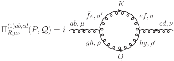
Refer to caption
Figure 3: Gluon-loop diagram contributing to the one-loop gluon self-energy.

We start by considering the gluon-loop diagram. Using the Feynman rules as given in Sec. II, it can be shown that66 6 To be more clear about the Lorentz and color indices used in Eq. (99), one can refer to Fig. 3.

ΠR;μ​ν(1)​a​b,c​d​(P,𝒬)\displaystyle\Pi^{(1)ab,cd}_{R;\mu\nu}(P,{\cal Q}) =\displaystyle= Π11;μ​ν(1)​a​b,c​d​(P,𝒬)+Π12;μ​ν(1)​a​b,c​d​(P,𝒬)\displaystyle\Pi^{(1)ab,cd}_{11;\mu\nu}(P,{\cal Q})+\Pi^{(1)ab,cd}_{12;\mu\nu}(P,{\cal Q}) (99)
=\displaystyle= i2​∑colors∫d4​K(2​π)4​[D11​(Q,𝒬g​h)​D11​(K,𝒬e​f)−D21​(Q,𝒬g​h)​D12​(K,𝒬e​f)]\displaystyle\frac{i}{2}\sum_{{\rm colors}}\int\frac{d^{4}K}{(2\pi)^{4}}\big[D_{11}(Q,{\cal Q}^{gh})D_{11}(K,{\cal Q}^{ef})-D_{21}(Q,{\cal Q}^{gh})D_{12}(K,{\cal Q}^{ef})\big]\,
×\displaystyle\times (−gσ​σ′)​(−gρ​ρ′)​𝒱L,μ​ρ​σa​b,e¯​f¯,g​h​(P,Q,K)​𝒱R,ν​ρ′​σ′c​d,g¯​h¯,e​f​(P,Q,K)​𝒫e​f,e¯​f¯​𝒫g​h,g¯​h¯,\displaystyle(-g^{\sigma\sigma^{\prime}})(-g^{\rho\rho^{\prime}}){\cal V}_{{\rm L},\,\mu\rho\sigma}^{ab,{\bar{e}}{\bar{f}},gh}(P,Q,K){\cal V}_{{\rm R},\,\nu\rho^{\prime}\sigma^{\prime}}^{cd,{\bar{g}}{\bar{h}},ef}(P,Q,K){\cal P}^{ef,{\bar{e}}{\bar{f}}}{\cal P}^{gh,{\bar{g}}{\bar{h}}}\,,

where K=P+QK=P+Q and the pre-factor 1/21/2 is the symmetry factor. In the above equation, all the color indices except aa, bb, cc and dd need to be summed. In addition, we use 𝒱L/R{\cal V}_{{\rm L}/{\rm R}} to denote the Feynman rules for the left and right vertex, respectively. Using the following identities

∑e¯​f¯fa​b,e¯​f¯,g​h​𝒫e​f,e¯​f¯=fa​b,f​e,g​h,∑g¯​h¯fc​d,g¯​h¯,e​f​𝒫g​h,g¯​h¯=fc​d,h​g,e​f,\sum_{{\bar{e}}{\bar{f}}}f^{ab,{\bar{e}}{\bar{f}},gh}{\cal P}^{ef,{\bar{e}}{\bar{f}}}=f^{ab,fe,gh}\,,\quad\sum_{{\bar{g}}{\bar{h}}}f^{cd,{\bar{g}}{\bar{h}},ef}{\cal P}^{gh,{\bar{g}}{\bar{h}}}=f^{cd,hg,ef}\,, (100)

where the two structure constants fa​b,e¯​f¯,g​hf^{ab,{\bar{e}}{\bar{f}},gh} and fc​d,g¯​h¯,e​ff^{cd,{\bar{g}}{\bar{h}},ef} come from the left and right vertex, respectively, the sum over color indices e¯{\bar{e}}, f¯{\bar{f}}, g¯{\bar{g}} and h¯{\bar{h}} can be carried out. In terms of the retarded/advanced and symmetric bare propagators, Eq. (99) can be expressed as

ΠR;μ​ν(1)​a​b,c​d​(P,𝒬)\displaystyle\Pi^{(1)ab,cd}_{R;\mu\nu}(P,{\cal Q}) =\displaystyle= i4​g2​∑colors∫d4​K(2​π)4​[DF​(Q,𝒬g​h)​DR​(K)+DA​(Q)​DF​(K,𝒬e​f)]\displaystyle\frac{i}{4}g^{2}\sum_{{\rm colors}}\int\frac{d^{4}K}{(2\pi)^{4}}\big[D_{F}(Q,{\cal Q}^{gh})D_{R}(K)+D_{A}(Q)D_{F}(K,{\cal Q}^{ef})\big]\, (101)
×\displaystyle\times fa​b,f​e,g​h​fc​d,h​g,e​f​ℒμ​ν(1)​(P,Q,K),\displaystyle f^{ab,fe,gh}f^{cd,hg,ef}{\cal L}^{(1)}_{\mu\nu}(P,Q,K)\,,

where the Lorentz structure is fully contained in ℒμ​ν(1)​(P,Q,K){\cal L}^{(1)}_{\mu\nu}(P,Q,K). Since it has nothing to do with the background field, a straightforward calculation gives that

ℒμ​ν(1)​(P,Q,K)\displaystyle{\cal L}^{(1)}_{\mu\nu}(P,Q,K) =\displaystyle= [(P+K)ρ​gμ​σ+(−K−Q)μ​gρ​σ+(Q−P)σ​gρ​μ]​gσ​σ′\displaystyle\big[(P+K)_{\rho}g_{\mu\sigma}+(-K-Q)_{\mu}g_{\rho\sigma}+(Q-P)_{\sigma}g_{\rho\mu}\big]g^{\sigma\sigma^{\prime}}
×\displaystyle\times [(−P+Q)σ′​gν​ρ′+(−Q−K)ν​gρ′​σ′+(K+P)ρ′​gσ′​ν]​gρ​ρ′\displaystyle\big[(-P+Q)_{\sigma^{\prime}}g_{\nu\rho^{\prime}}+(-Q-K)_{\nu}g_{\rho^{\prime}\sigma^{\prime}}+(K+P)_{\rho^{\prime}}g_{\sigma^{\prime}\nu}\big]g^{\rho\rho^{\prime}}
=\displaystyle= [(P+K)2+(P−Q)2]​gμ​ν+10​Kμ​Kν−5​(Kμ​Pν+Kν​Pμ)−2​Pμ​Pν.\displaystyle\big[(P+K)^{2}+(P-Q)^{2}\big]g_{\mu\nu}+10K_{\mu}K_{\nu}-5(K_{\mu}P_{\nu}+K_{\nu}P_{\mu})-2P_{\mu}P_{\nu}\,.

Turning to the ghost-loop diagram [see Fig. 2 (c)], the corresponding calculation is very similar to the above. It is easy to show the following:

ΠR;μ​ν(2)​a​b,c​d​(P,𝒬)\displaystyle\Pi^{(2)ab,cd}_{R;\mu\nu}(P,{\cal Q}) =\displaystyle= −i4g2∑colors∫d4​K(2​π)4[DF(Q,𝒬g​h)DR(K)+DA(Q)DF(K,𝒬e​f)]\displaystyle-\frac{i}{4}g^{2}\sum_{{\rm colors}}\int\frac{d^{4}K}{(2\pi)^{4}}\big[D_{F}(Q,{\cal Q}^{gh})D_{R}(K)+D_{A}(Q)D_{F}(K,{\cal Q}^{ef})\big]\, (103)
×\displaystyle\times fa​b,f​e,g​h​fc​d,h​g,e​f​2​Kμ​Qν.\displaystyle f^{ab,fe,gh}f^{cd,hg,ef}2K_{\mu}Q_{\nu}\,.

In order to get a final result as given by Eq. (45), we need to rewrite the above equation with a more symmetric form. By changing the variables Q→−K′Q\rightarrow-K^{\prime} and K→−Q′K\rightarrow-Q^{\prime}, we can show that

∫d4​K(2​π)4​[DF​(Q,𝒬g​h)​DR​(K)+DA​(Q)​DF​(K,𝒬e​f)]​Kμ​Qν\displaystyle\int\frac{d^{4}K}{(2\pi)^{4}}\big[D_{F}(Q,{\cal Q}^{gh})D_{R}(K)+D_{A}(Q)D_{F}(K,{\cal Q}^{ef})\big]K_{\mu}Q_{\nu}
=∫d4​Q′(2​π)4​[DF​(−K′,𝒬g​h)​DR​(−Q′)+DA​(−K′)​DF​(−Q′,𝒬e​f)]​Qμ′​Kν′\displaystyle=\int\frac{d^{4}Q^{\prime}}{(2\pi)^{4}}\big[D_{F}(-K^{\prime},{\cal Q}^{gh})D_{R}(-Q^{\prime})+D_{A}(-K^{\prime})D_{F}(-Q^{\prime},{\cal Q}^{ef})\big]Q^{\prime}_{\mu}K^{\prime}_{\nu}
=∫d4​K′(2​π)4​[DF​(K′,𝒬h​g)​DA​(Q′)+DR​(K′)​DF​(Q′,𝒬f​e)]​Qμ′​Kν′,\displaystyle=\int\frac{d^{4}K^{\prime}}{(2\pi)^{4}}\big[D_{F}(K^{\prime},{\cal Q}^{hg})D_{A}(Q^{\prime})+D_{R}(K^{\prime})D_{F}(Q^{\prime},{\cal Q}^{fe})\big]Q^{\prime}_{\mu}K^{\prime}_{\nu}\,, (104)

where we changed d4​Q′d^{4}Q^{\prime} into d4​K′d^{4}K^{\prime} because K′=P+Q′K^{\prime}=P+Q^{\prime}. In addition, under the sign change of the momentum in the symmetric propagator, the flip of the color indices in the last line in Eq. (A) is due to the definition of the distribution function as given by Eq. (13). By realizing the fact that the product of the two structure constants in Eq. (103) is invariant under the interchanges of color indices, h↔eh\leftrightarrow e and g↔fg\leftrightarrow f, it can be shown that

ΠR;μ​ν(2)​a​b,c​d​(P,𝒬)\displaystyle\Pi^{(2)ab,cd}_{R;\mu\nu}(P,{\cal Q}) =\displaystyle= i4​g2​∑colors∫d4​K(2​π)4​[DF​(Q,𝒬g​h)​DR​(K)+DA​(Q)​DF​(K,𝒬e​f)]\displaystyle\frac{i}{4}g^{2}\sum_{{\rm colors}}\int\frac{d^{4}K}{(2\pi)^{4}}\big[D_{F}(Q,{\cal Q}^{gh})D_{R}(K)+D_{A}(Q)D_{F}(K,{\cal Q}^{ef})\big]\, (105)
×\displaystyle\times fa​b,f​e,g​h​fc​d,h​g,e​f​ℒμ​ν(2)​(P,Q,K),\displaystyle f^{ab,fe,gh}f^{cd,hg,ef}{\cal L}^{(2)}_{\mu\nu}(P,Q,K)\,,

where

ℒμ​ν(2)(P,Q,K)=−(2KμQν+2QμKν)/2=−2KμKν+PμKν+KμPν.{\cal L}^{(2)}_{\mu\nu}(P,Q,K)=-(2K_{\mu}Q_{\nu}+2Q_{\mu}K_{\nu})/2=-2K_{\mu}K_{\nu}+P_{\mu}K_{\nu}+K_{\mu}P_{\nu}\,. (106)

Finally, we consider the tadpole diagram [see Fig. 2 (d)] which can be expressed as

ΠR;μ​ν(3)​a​b,c​d​(P,𝒬)=34​g2​∑colors∫d4​K(2​π)4​DF​(K,𝒬e​f)​(fa​b,e​f,i​j​fc​d,j​i,f​e−fa​b,f​e,i​j​fc​d,e​f,j​i)​gμ​ν.\Pi^{(3)ab,cd}_{R;\mu\nu}(P,{\cal Q})=\frac{3}{4}g^{2}\sum_{{\rm colors}}\int\frac{d^{4}K}{(2\pi)^{4}}D_{F}(K,{\cal Q}^{ef})(f^{ab,ef,ij}f^{cd,ji,fe}-f^{ab,fe,ij}f^{cd,ef,ji})g_{\mu\nu}\,. (107)

Notice that one of the three terms in the four-gluon vertex (see the Feynman rules in Fig. 1) vanishes because ∑g​hfi​j,e​f,g​h​𝒫e​f,g​h=0\sum_{gh}f^{ij,ef,gh}{\cal P}^{ef,gh}=0 where the projection operator comes from the gluon propagator. Clearly, the above equation needs to be rewritten in a form analogous to the corresponding results from the other two Feynman diagrams. To do so, we first express Eq. (107) in the following form:

ΠR;μ​ν(3)​a​b,c​d​(P,𝒬)=34​g2​∑colors∫d4​K(2​π)4​[DF​(Q,𝒬f​e)+DF​(K,𝒬e​f)]​fa​b,f​e,i​j​fc​d,j​i,e​f​gμ​ν.\Pi^{(3)ab,cd}_{R;\mu\nu}(P,{\cal Q})=\frac{3}{4}g^{2}\sum_{{\rm colors}}\int\frac{d^{4}K}{(2\pi)^{4}}\big[D_{F}(Q,{\cal Q}^{fe})+D_{F}(K,{\cal Q}^{ef})\big]f^{ab,fe,ij}f^{cd,ji,ef}g_{\mu\nu}\,. (108)

To get the above equation, the color indices ee and ff in DF​(K,𝒬e​f)​fa​b,e​f,i​j​fc​d,j​i,f​eD_{F}(K,{\cal Q}^{ef})f^{ab,ef,ij}f^{cd,ji,fe} in Eq. (107) have been interchanged, and the resulting DF​(K,𝒬f​e)D_{F}(K,{\cal Q}^{fe}) is then replaced by DF​(Q,𝒬f​e)D_{F}(Q,{\cal Q}^{fe}) which is valid under the integral ∫d4​K\int d^{4}K. Furthermore, for the contribution associated with DF​(Q,𝒬f​e)D_{F}(Q,{\cal Q}^{fe}), we can insert a term −i​DR​(K)​(K2+Q2)-iD_{R}(K)(K^{2}+Q^{2}) into Eq. (108) because such an inserted term is effectively “11 ” under the integral thanks to the delta function in the propagator. Similarly, a term −i​DA​(Q)​(K2+Q2)-iD_{A}(Q)(K^{2}+Q^{2}) can be also inserted into the above equation for the contribution associated with DF​(K,𝒬e​f)D_{F}(K,{\cal Q}^{ef}). Consequently, we arrive at

ΠR;μ​ν(3)​a​b,c​d​(P,𝒬)\displaystyle\Pi^{(3)ab,cd}_{R;\mu\nu}(P,{\cal Q}) =\displaystyle= i4​g2​∑colors∫d4​K(2​π)4​[DF​(Q,𝒬g​h)​DR​(K)+DA​(Q)​DF​(K,𝒬e​f)]\displaystyle\frac{i}{4}g^{2}\sum_{{\rm colors}}\int\frac{d^{4}K}{(2\pi)^{4}}\big[D_{F}(Q,{\cal Q}^{gh})D_{R}(K)+D_{A}(Q)D_{F}(K,{\cal Q}^{ef})\big]\, (109)
×\displaystyle\times fa​b,f​e,g​h​fc​d,h​g,e​f​ℒμ​ν(3)​(P,Q,K),\displaystyle f^{ab,fe,gh}f^{cd,hg,ef}{\cal L}^{(3)}_{\mu\nu}(P,Q,K)\,,

with ℒμ​ν(3)​(P,Q,K)=−3​(K2+Q2)​gμ​ν{\cal L}^{(3)}_{\mu\nu}(P,Q,K)=-3(K^{2}+Q^{2})g_{\mu\nu}.

Summing up the above results, the total contribution from the pure gauge part to the retarded gluon self-energy reads

ΠR;μ​νa​b,c​d​(P,𝒬)\displaystyle\Pi^{ab,cd}_{R;\mu\nu}(P,{\cal Q}) =\displaystyle= i4​g2​∑colors∫d4​K(2​π)4​[DF​(Q,𝒬g​h)​DR​(K)+DA​(Q)​DF​(K,𝒬e​f)]\displaystyle\frac{i}{4}g^{2}\sum_{{\rm colors}}\int\frac{d^{4}K}{(2\pi)^{4}}\big[D_{F}(Q,{\cal Q}^{gh})D_{R}(K)+D_{A}(Q)D_{F}(K,{\cal Q}^{ef})\big]\, (110)
×\displaystyle\times fa​b,f​e,g​h​fc​d,h​g,e​f​ℒμ​ν​(P,Q,K),\displaystyle f^{ab,fe,gh}f^{cd,hg,ef}{\cal L}_{\mu\nu}(P,Q,K)\,,

where

ℒμ​ν​(P,Q,K)\displaystyle{\cal L}_{\mu\nu}(P,Q,K) =\displaystyle= ℒμ​ν(1)​(P,Q,K)+ℒμ​ν(2)​(P,Q,K)+ℒμ​ν(3)​(P,Q,K)\displaystyle{\cal L}^{(1)}_{\mu\nu}(P,Q,K)+{\cal L}^{(2)}_{\mu\nu}(P,Q,K)+{\cal L}^{(3)}_{\mu\nu}(P,Q,K) (111)
≈\displaystyle\approx 8​Kμ​Kν−4​Kμ​Pν−4​Pμ​Kν−4​Q⋅K​gμ​ν.\displaystyle 8K_{\mu}K_{\nu}-4K_{\mu}P_{\nu}-4P_{\mu}K_{\nu}-4Q\cdot Kg_{\mu\nu}\,.

Here, we drop terms ∼Pμ​Pν\sim P_{\mu}P_{\nu} which give contributions beyond NLO in the HTL approximation. At this point, it is clear to see Eq. (110) is identical to Eq. (45).

Given the above calculations, the corresponding contributions to the symmetric gluon self-energy from Figs. 2 (b), 2 (c) and 2 (d) can be obtained straightforwardly. Notice that the tadpole diagram does not contribute to ΠF;μ​νa​b,c​d​(P,𝒬)\Pi^{ab,cd}_{F;\mu\nu}(P,{\cal Q}). However, in order to show its similarity with Eq. (109), we can write such a zero result as

ΠF;μ​ν(3)​a​b,c​d​(P,𝒬)\displaystyle\Pi^{(3)ab,cd}_{F;\mu\nu}(P,{\cal Q}) =\displaystyle= i4g2∑colors∫d4​K(2​π)4[DF(Q,𝒬g​h)DF(K,𝒬e​f)−(DR(K)−DA(K))\displaystyle\frac{i}{4}g^{2}\sum_{{\rm colors}}\int\frac{d^{4}K}{(2\pi)^{4}}\big[D_{F}(Q,{\cal Q}^{gh})D_{F}(K,{\cal Q}^{ef})-\big(D_{R}(K)-D_{A}(K)\big)\, (112)
×\displaystyle\times (DR(Q)−DA(Q))]fa​b,f​e,g​hfc​d,h​g,e​f(−3)(K2+Q2)gμ​ν.\displaystyle\big(D_{R}(Q)-D_{A}(Q)\big)\big]f^{ab,fe,gh}f^{cd,hg,ef}(-3)(K^{2}+Q^{2})g_{\mu\nu}\,.

The above equation vanishes due to a product of delta functions δ⁡(K2)​δ​(Q2)\delta(K^{2})\delta(Q^{2}) from the propagators. As a result, the symmetric gluon self-energy ΠF;μ​ν(i)​a​b,c​d​(P,𝒬)\Pi^{(i)ab,cd}_{F;\mu\nu}(P,{\cal Q}) with i=1,2,3i=1,2,3 can be simply obtained from the retarded solutions ΠR;μ​ν(i)​a​b,c​d​(P,𝒬)\Pi^{(i)ab,cd}_{R;\mu\nu}(P,{\cal Q}) as given in Eqs. (101), (105) and (109) by the following replacement:

DF​(Q,𝒬g​h)​DR​(K)+DA​(Q)​DF​(K,𝒬e​f)\displaystyle D_{F}(Q,{\cal Q}^{gh})D_{R}(K)+D_{A}(Q)D_{F}(K,{\cal Q}^{ef})
⟶DF​(Q,𝒬g​h)​DF​(K,𝒬e​f)−(DR​(K)−DA​(K))​(DR​(Q)−DA​(Q)).\displaystyle\quad\longrightarrow D_{F}(Q,{\cal Q}^{gh})D_{F}(K,{\cal Q}^{ef})-\big(D_{R}(K)-D_{A}(K)\big)\big(D_{R}(Q)-D_{A}(Q)\big)\,. (113)

Thus, up to NLO in the HTL approximation, the three diagrams in the pure gauge part lead to the following contributions to the symmetric gluon self-energy

ΠF;μ​νa​b,c​d​(P,𝒬)=i​g2​∑e​f​g​hfa​b,f​e,g​h​fc​d,h​g,e​f​∫d4​K(2​π)4​(2​Kμ​Kν−Pμ​Kν−Kμ​Pν−gμ​ν​Q⋅K)\displaystyle\Pi^{ab,cd}_{F;\mu\nu}(P,{\cal Q})=ig^{2}\sum_{efgh}f^{ab,fe,gh}f^{cd,hg,ef}\int\frac{d^{4}K}{(2\pi)^{4}}(2K_{\mu}K_{\nu}-P_{\mu}K_{\nu}-K_{\mu}P_{\nu}-g_{\mu\nu}Q\cdot K)\,
×[DF​(Q,𝒬g​h)​DF​(K,𝒬e​f)−(DR​(K)−DA​(K))​(DR​(Q)−DA​(Q))].\displaystyle\quad\times\big[D_{F}(Q,{\cal Q}^{gh})D_{F}(K,{\cal Q}^{ef})-\big(D_{R}(K)-D_{A}(K)\big)\big(D_{R}(Q)-D_{A}(Q)\big)\big]\,. (114)

As we can see, the above equation is analogous to the quark-loop contribution to ΠF;μ​νa​b,c​d​(P,𝒬)\Pi^{ab,cd}_{F;\mu\nu}(P,{\cal Q}) which is given by Eq. (57).

Appendix B REORGANIZATION OF THE LO SYMMETRIC GLUON SELF-ENERGY

As shown in Eqs. (56) and (68), both the NLO ΠR/A\Pi_{R/A} and the LO ΠF\Pi_{F} can reproduce the correct limit at 𝒬=0{\cal Q}=0. For nonzero background field, however, they get different modifications on the Debye mass. In fact, such a background field modification originates from the integral over kk where the integrand of the retarded solution consists of a sum of two distribution functions, see Eq. (III). On the other hand, according to Eq. (61), the corresponding integral in the symmetric solution involves a more complicated combination of the distribution functions. In order to show more similarities between the two, it appears to be interesting to artificially introduce a term to the LO symmetric gluon self-energy which vanishes at 𝒬=0{\cal Q}=0, and thus gives the anomalous contribution. Subtracting it from Eq. (IV.1), we can define the so-called normal contribution.

Taking the fermionic part [Eq. (61)] as an example, explicitly, we can write

ΠF;μ​νano​(P,𝒬)\displaystyle\Pi^{\rm ano}_{F;\mu\nu}(P,{\cal Q}) =\displaystyle= −ig24​π2​pNfδa​dδb​c∫k2dk[(n~+a(k)−n~+c(k))2+(n~−a(k)−n~−c(k))2]Λμ​ν(P)\displaystyle-i\frac{g^{2}}{4\pi^{2}p}N_{f}\delta^{ad}\delta^{bc}\int k^{2}dk[({\tilde{n}}_{+}^{a}(k)-{\tilde{n}}_{+}^{c}(k))^{2}+({\tilde{n}}_{-}^{a}(k)-{\tilde{n}}_{-}^{c}(k))^{2}]\Lambda_{\mu\nu}(P)\, (115)
=\displaystyle= i​Tp​mf2​δa​d​δb​c​[ℱf(1)​(𝗊a,𝗊c)+12​cot⁡(π​𝗊a​c)​𝒢f​(𝗊a,𝗊c)]​Λμ​ν​(P),\displaystyle i\frac{T}{p}m_{f}^{2}\delta^{ad}\delta^{bc}\big[{\cal F}_{f}^{(1)}({\sf q}^{a},{\sf q}^{c})+\frac{1}{2}\cot(\pi{\sf q}^{ac}){\cal G}_{f}({\sf q}^{a},{\sf q}^{c})\big]\Lambda_{\mu\nu}(P)\,,\

and

ΠF;μ​νnor(P,𝒬)=ig2​T4​π2​pNf∫kdk{δa​bδc​d4N[n~+a(k)+n~−a(k)+n~+c(k)+n~−c(k)\displaystyle\Pi^{\rm nor}_{F;\mu\nu}(P,{\cal Q})=i\frac{g^{2}T}{4\pi^{2}p}N_{f}\int kdk\Big\{\delta^{ab}\delta^{cd}\frac{4}{N}\Big[{\tilde{n}}_{+}^{a}(k)+{\tilde{n}}_{-}^{a}(k)+{\tilde{n}}_{+}^{c}(k)+{\tilde{n}}_{-}^{c}(k)\,
−1N∑e(n~+e(k)+n~−e(k))]−2δa​dδb​c(n~+a(k)+n~−a(k)+n~+c(k)+n~−c(k))}Λμ​ν(P)\displaystyle\quad-\frac{1}{N}\sum_{e}({\tilde{n}}_{+}^{e}(k)+{\tilde{n}}_{-}^{e}(k))\Big]-2\delta^{ad}\delta^{bc}\big({\tilde{n}}_{+}^{a}(k)+{\tilde{n}}_{-}^{a}(k)+{\tilde{n}}_{+}^{c}(k)+{\tilde{n}}_{-}^{c}(k)\big)\Big\}\Lambda_{\mu\nu}(P)\,
=i​Tp​mf2​[δa​b​δc​d​1N​ℱf(2)​(𝗊a,𝗊c)−δa​d​δb​c​ℱf(1)​(𝗊a,𝗊c)]​Λμ​ν​(P).\displaystyle\quad=i\frac{T}{p}m_{f}^{2}\Big[\delta^{ab}\delta^{cd}\frac{1}{N}{\cal F}^{(2)}_{f}({\sf q}^{a},{\sf q}^{c})-\delta^{ad}\delta^{bc}{\cal F}^{(1)}_{f}({\sf q}^{a},{\sf q}^{c})\Big]\Lambda_{\mu\nu}(P)\,. (116)

The above anomalous contribution shares some similarities with ΠR;μ​νano​(P,𝒬)\Pi^{\rm ano}_{R;\mu\nu}(P,{\cal Q}) as given in Eq. (51). They both come from the LO terms in the HTL approximation and contain only the off-diagonal components. In addition, the anomalous contribution vanishes when 𝒬=0{\cal Q}=0 or 𝗊a=𝗊c{\sf q}^{a}={\sf q}^{c} because a difference between two distribution functions appears in the integrand in Eq. (115). Similar as before, to avoid an “∞⋅0\infty\cdot 0 ” ambiguity in our analytical result, 𝗊a=𝗊c{\sf q}^{a}={\sf q}^{c} should be understood as 𝗊a→𝗊c±ϵ{\sf q}^{a}\rightarrow{\sf q}^{c}\pm\epsilon. Then the second line in Eq. (115) equals zero as expected. However, different from Eq. (51), such an artificially introduced anomalous contribution is orthogonal to PμP^{\mu} and does not satisfy a similar relation as given by Eq. (53).

Although it is trivial to show that the sum of Eqs. (115) and (B) is identical to Eq. (63), the motivation for separating Eq. (61) into the above two parts becomes clear when we look at the normal contributions. According to Eqs. (52) and (B), the background field modification on mf2m_{f}^{2} which involves only B2​(x)B_{2}(x) is exactly the same for both the retarded/advanced and symmetric gluon self-energies. Consequently, the 𝒬{\cal Q}-dependent mass squared as defined in Eq. (54) is universal to describe the background field modification on the normal contributions in all the three independent real-time gluon self-energies. Furthermore, it also turns out to be meaningful when we include nonperturbative contributions in the gluon self-energy which however, is beyond the scope of current work and we only provide a very preliminary discussion at the end of Sec. VI.

A similar consideration also applies to the pure gauge part and the corresponding anomalous and normal contributions are given by the following equations:

ΠF;μ​νano​(P,𝒬)\displaystyle\Pi^{\rm ano}_{F;\mu\nu}(P,{\cal Q}) =\displaystyle= i​Tp​mg2​δa​d​δb​c​[ℱg(1)​(𝗊a,𝗊c)−12​cot⁡(π​𝗊a​c)​𝒢g​(𝗊a,𝗊c)]​Λμ​ν​(P),\displaystyle i\frac{T}{p}m_{g}^{2}\delta^{ad}\delta^{bc}\big[{\cal F}_{g}^{(1)}({\sf q}^{a},{\sf q}^{c})-\frac{1}{2}\cot(\pi{\sf q}^{ac}){\cal G}_{g}({\sf q}^{a},{\sf q}^{c})\big]\Lambda_{\mu\nu}(P)\,, (117)
ΠF;μ​νnor​(P,𝒬)\displaystyle\Pi^{\rm nor}_{F;\mu\nu}(P,{\cal Q}) =\displaystyle= i​Tp​mg2​[δa​b​δc​d​1N​ℱg(2)​(𝗊a,𝗊c)−δa​d​δb​c​ℱg(1)​(𝗊a,𝗊c)]​Λμ​ν​(P).\displaystyle i\frac{T}{p}m_{g}^{2}\Big[\delta^{ab}\delta^{cd}\frac{1}{N}{\cal F}^{(2)}_{g}({\sf q}^{a},{\sf q}^{c})-\delta^{ad}\delta^{bc}{\cal F}^{(1)}_{g}({\sf q}^{a},{\sf q}^{c})\Big]\Lambda_{\mu\nu}(P)\,. (118)

Finally, we can also express the normal contributions of the LO symmetric gluon self-energy as

ΠF;μ​νnor​(P,𝒬)=−i​Tp​(ℳD2)a​b,c​d​(𝒬)​Λμ​ν​(P),\Pi^{\rm nor}_{F;\mu\nu}(P,{\cal Q})=-i\frac{T}{p}({\cal M}_{D}^{2})^{ab,cd}({\cal Q})\Lambda_{\mu\nu}(P)\,, (119)

where (ℳD2)a​b,c​d​(𝒬)({\cal M}_{D}^{2})^{ab,cd}({\cal Q}) has been already defined in Eq. (54).

References

  • (1) J. I. Kapusta, Quantum chromodynamics at high temperature, Nucl. Phys. B148, 461 (1979).
  • (2) K. Kajantie, M. Laine, K. Rummukainen and Y. Schroder, The pressure of hot QCD up to g6 ln(1/g), Phys. Rev. D 67, 105008 (2003).
  • (3) J. O. Andersen, M. Strickland and N. Su, Gluon Thermodynamics at Intermediate Coupling, Phys. Rev. Lett. 104, 122003 (2010).
  • (4) Y. Hidaka and R. D. Pisarski, Suppression of the shear viscosity in a ”semi” quark gluon plasma, Phys. Rev. D 78, 071501 (2008).
  • (5) G. Boyd, J. Engels, F. Karsch, E. Laermann, C. Legeland, M. Lutgemeier and B. Petersson, Thermodynamics of SU(3) lattice gauge theory, Nucl. Phys. B469, 419(1996).
  • (6) S. Borsanyi, G. Endrodi, Z. Fodor, S. D. Katz and K. K. Szabo, Precision SU(3) lattice thermodynamics for a large temperature range, J. High Energy Phys. 07 (2012) 056.
  • (7) M. Panero, Thermodynamics of the QCD Plasma and the Large-N limit, Phys. Rev. Lett. 103, 232001 (2009).
  • (8) A. Bazavov, T. Bhattacharya, M. Cheng, N. H. Christ, C. DeTar, S. Ejiri, S. Gottlieb, R. Gupta, U. M. Heller, K. Huebner, et al., Equation of state and QCD transition at finite temperature, Phys. Rev. D 80, 014504 (2009).
  • (9) S. Borsanyi, G. Endrodi, Z. Fodor, A. Jakovac, S. D. Katz, S. Krieg, C. Ratti and K. K. Szabo, The QCD equation of state with dynamical quarks, J. High Energy Phys. 11 (2010) 077.
  • (10) O. Kaczmarek, F. Karsch, P. Petreczky and F. Zantow, Heavy quark anti-quark free energy and the renormalized Polyakov loop, Phys. Lett. B 543, 41(2002).
  • (11) P. Petreczky and K. Petrov, Free energy of a static quark anti-quark pair and the renormalized Polyakov loop in three flavor QCD, Phys. Rev. D 70, 054503 (2004).
  • (12) S. Gupta, K. Huebner and O. Kaczmarek, Renormalized Polyakov loops in many representations, Phys. Rev. D 77, 034503 (2008).
  • (13) V. M. Belyaev, Order parameter and effective potential, Phys. Lett. B 254, 153 (1991).
  • (14) T. Bhattacharya, A. Gocksch, C. Korthals Altes and R. D. Pisarski, Z(N) interface tension in a hot SU(N) gauge theory, Nucl. Phys. B383, 497 (1992).
  • (15) C. P. Korthals Altes, Constrained effective potential in hot QCD, Nucl. Phys. B420, 637 (1994).
  • (16) C. P. Korthals Altes, R. D. Pisarski and A. Sinkovics, The potential for the phase of the Wilson line at nonzero quark density, Phys. Rev. D 61, 056007 (2000).
  • (17) A. Dumitru, Y. Guo and C. P. Korthals Altes, Two-loop perturbative corrections to the thermal effective potential in gluodynamics, Phys. Rev. D 89, 016009 (2014).
  • (18) U. Reinosa, J. Serreau, M. Tissier and N. Wschebor, Two-loop study of the deconfinement transition in Yang-Mills theories: SU(3) and beyond, Phys. Rev. D 93, 105002 (2016).
  • (19) J. Maelger, U. Reinosa and J. Serreau, Perturbative study of the QCD phase diagram for heavy quarks at nonzero chemical potential: Two-loop corrections, Phys. Rev. D 97, 074027 (2018).
  • (20) Y. Guo and Q. Du, Two-loop perturbative corrections to the constrained effective potential in thermal QCD, J. High Energy Phys. 05 (2019) 042.
  • (21) P. N. Meisinger, T. R. Miller and M. C. Ogilvie, Phenomenological equations of state for the quark gluon plasma, Phys. Rev. D 65, 034009 (2002)
  • (22) A. Dumitru, Y. Guo, Y. Hidaka, C. P. K. Altes and R. D. Pisarski, How Wide is the transition to deconfinement?, Phys. Rev. D 83, 034022 (2011).
  • (23) A. Dumitru, Y. Guo, Y. Hidaka, C. P. K. Altes and R. D. Pisarski, Effective matrix model for deconfinement in pure gauge theories, Phys. Rev. D 86, 105017 (2012).
  • (24) R. D. Pisarski and V. V. Skokov, Gross-Witten-Wadia transition in a matrix model of deconfinement, Phys. Rev. D 86, 081701 (2012).
  • (25) Y. Guo, Matrix models for deconfinement and their perturbative corrections, J. High Energy Phys. 11 (2014)111.
  • (26) R. D. Pisarski and V. V. Skokov, Chiral matrix model of the semi-QGP in QCD, Phys. Rev. D 94, 034015 (2016)
  • (27) Y. Hidaka and R. D. Pisarski, Small shear viscosity in the semi quark gluon plasma, Phys. Rev. D 81, 076002 (2010).
  • (28) C. Gale, Y. Hidaka, S. Jeon, S. Lin, J. F. Paquet, R. D. Pisarski, D. Satow, V. V. Skokov and G. Vujanovic, Production and Elliptic Flow of Dileptons and Photons in a Matrix Model of the Quark-Gluon Plasma, Phys. Rev. Lett. 114, 072301 (2015).
  • (29) Y. Hidaka, S. Lin, R. D. Pisarski and D. Satow, Dilepton and photon production in the presence of a nontrivial Polyakov loop, J. High Energy Phys. 10 (2015) 005.
  • (30) B. Singh, A. Abhishek, S. K. Das and H. Mishra, Heavy quark diffusion in a Polyakov loop plasma, Phys. Rev. D 100, 114019 (2019).
  • (31) B. Singh and H. Mishra, Heavy quark transport in a viscous semi QGP, Phys. Rev. D 101, 054027 (2020)
  • (32) S. Lin, R. D. Pisarski and V. V. Skokov, Collisional energy loss above the critical temperature in QCD, Phys. Lett. B 730, 236 (2014).
  • (33) E. Braaten and R. D. Pisarski, Soft Amplitudes in Hot Gauge Theories: A General Analysis, Nucl. Phys. B337, 569 (1990).
  • (34) M. L. Bellac, Thermal Field Theory, Cambridge University Press, Cambridge, England 2011.
  • (35) P. Romatschke and M. Strickland, Collective modes of an anisotropic quark gluon plasma, Phys. Rev. D 68, 036004 (2003).
  • (36) P. Romatschke and M. Strickland, Collective modes of an anisotropic quark-gluon plasma II, Phys. Rev. D 70, 116006 (2004).
  • (37) Q. Du, A. Dumitru, Y. Guo and M. Strickland, Bulk viscous corrections to screening and damping in QCD at high temperatures, J. High Energy Phys. 01 (2017) 123.
  • (38) Y. Hidaka and R. D. Pisarski, Hard thermal loops, to quadratic order, in the background of a spatial ’t Hooft loop, Phys. Rev. D 80, 036004 (2009); Erratum, Phys. Rev. D 102, 059902 (2020).
  • (39) L. V. Keldysh, Diagram technique for nonequilibrium processes, Sov. Phys. JETP 20, 1018 (1965).
  • (40) R. Kubo, Statistical mechanical theory of irreversible processes. 1. General theory and simple applications in magnetic and conduction problems, J. Phys. Soc. Jpn. 12, 570 (1957).
  • (41) P. C. Martin and J. S. Schwinger, Theory of many particle systems. 1., Phys. Rev. 115, 1342 (1959).
  • (42) P. Cvitanovic, Group theory for Feynman diagrams in non-Abelian gauge theories, Phys. Rev. D 14, 1536 (1976).
  • (43) Y. Guo and Z. Kuang, Resummed gluon propagator and Debye screening effect in a holonomous plasma, Phys. Rev. D 104, 014015 (2021).
  • (44) K. Furuuchi, Confined phase in real time formalism and the fate of the world behind the horizon, Phys. Rev. D 73, 046004 (2006).
  • (45) C. P. Korthals Altes, H. Nishimura, R. D. Pisarski and V. V. Skokov, Conundrum for the free energy of a holonomous gluonic plasma at cubic order, Phys. Lett. B 803, 135336 (2020).
  • (46) C. P. Korthals Altes, H. Nishimura, R. D. Pisarski and V. V. Skokov, Free energy of a holonomous plasma, Phys. Rev. D 101, 094025 (2020).
  • (47) Y. Hidaka and R. D. Pisarski, Effective models of a semi-quark-gluon plasma, Phys. Rev. D 104, 074036 (2021).