Rotational pendulum dynamics of a vortex molecule in a channel geometry
Abstract
A vortex molecule is a topological excitation in two coherently coupled superfluids consisting of a vortex in each superfluid connected by a domain wall of the relative phase, also known as a Josephson vortex. We investigate the dynamics of this excitation in a quasi-two-dimensional geometry with slab or channel boundary conditions using an extended point vortex framework complemented by Gross-Pitaevskii simulations. Apart from translational motion along the channel, the vortex molecule is found to exhibit intriguing internal dynamics including rotation and rotational-pendulum-like dynamics. Trajectories leading to a boundary-induced break-up of the vortex molecule are also described qualitatively by the simplified model. We classify the stable and unstable fixed points as well as separatrices that characterize the vortex molecule dynamics.
Keywords:
coherently coupled Bose-Einstein condensates, fractional vortex molecule, coreless vortex, solitonic vortexI Introduction
Nonlinear topological excitations like vortices have been the topic of study in many fields ranging from high-energy to condensed-matter physics Thouless 1998; Manton and Sutcliffe 2004. They are long lived and stable due to protection by topological constraints and can only be destroyed by annihilation with opposite charges, or by moving out of the superfluid domain. Intriguing examples of topological excitations are vortex molecules García-Ripoll et al. 2002; Kasamatsu et al. 2004, which exist in two-component superfluids with linear coupling.
Recent experimental progress has made it possible to study two-dimensional two-component Bose-Einstein condensates (BECs) with homogeneous linear (Rabi) coupling between the two components Nicklas et al. 2015; Farolfi et al. 2021a; Farolfi et al. 2021b, thus creating an extended linearly-coupled two-component superfluid. The linear coupling tends to align the phases of the two condensates. As such, a vortex filament piercing only one of the two condensates initiates a domain wall of the relative phase Son and Stephanov 2002, which can terminate at an antivortex in the same condensate, or at a vortex in the other one. The latter situation is referred to as a vortex molecule Kasamatsu et al. 2004, or sometimes a fractional vortex molecule Eto et al. 2020, since either of the two individual vortices only carries a fraction of the total vortex charge. Vortex molecules have been studied extensively in the theoretical literature García-Ripoll et al. 2002; Kasamatsu et al. 2004; Cipriani and Nitta 2013; Tylutki et al. 2016; Kasamatsu et al. 2016; Calderaro et al. 2017. Interest in vortex molecules is partly motivated by the fact that the domain wall creates an energy cost that is approximately linear with the separation of the two vortices, which evokes analogies to color confinement in quantum chromodynamics Eto and Nitta 2018; Eto et al. 2020.
Predicting and understanding vortex dynamics is a challenging problem. A ubiquitous situation in ultracold gas experiments is the elongated or cigar-shaped geometry Ketterle and Zwierlein 2008; Pethick and Smith 2008; Becker et al. 2013, where a vortex perpendicular to the long trap axis is a stable nonlinear excitation in a scalar superfluid Muñoz Mateo and Brand 2015. In such an elongated trap, a single vortex becomes a localised excitation on the length scale of the narrow trap diameter resembling a dark soliton, which gives rise to the concept of a solitonic vortex Brand and Reinhardt 2001; Brand and Reinhardt 2002; Komineas and Papanicolaou 2003; Yefsah et al. 2013; Ku et al. 2014; Donadello et al. 2014; Toikka and Brand 2017.
In this work we analyse the motion of a vortex molecule in a channel, or slab geometry that is extended in one dimension and has parallel hard-wall boundaries in the second. We assume the third dimension to be tightly confined to the order of the healing length or smaller, such that the problem effectively becomes two-dimensional. This channel geometry embodies the essential qualitative features of the ubiquitous elongated atom trap, while at the same time providing access to analytical treatment. Furthermore, near homogeneous potentials with hard walls, so-called flat bottom traps, have become increasingly available to experiments in recent years Chomaz et al. 2015; Kwon et al. 2021.
The dynamics of a single vortex in a channel was analysed in Ref. Toikka and Brand 2017 starting from the method of images and applying compressible corrections as a perturbation. For a vortex molecule, the presence of the domain wall connecting the vortices provides an interaction potential, which has an interesting interplay with the effects of the channel boundaries on the vortex motion. Here, we develop a simple model for the dynamics of a vortex molecule augmenting the method of images by a parameterised interaction potential capturing the effects of the domain wall. Similar ideas have previously been implemented to understand the rotation dynamics of a centered vortex molecule in an isotropic harmonic trap Tylutki et al. 2016; Calderaro et al. 2017. For the channel geometry the model predicts a rich phase space for the vortex molecule dynamics with different dynamical regimes separated by separatices. A particularly intriguing rotational-pendulum-like regime of motion is predicted in the case of repulsive cross-condensate nonlinear interactions where the vortex-vortex interaction has a minimum at finite vortex separation. Numerical simulations with the Gross-Pitaevskii equation (GPE) complement and support the predictions of the simplified model.
The paper is structured as follows. Section II introduces the system in light of the GPE. Section III introduces the main point-vortex model and its equations of motion. Section IV discusses the resulting dynamics of the vortex molecule comparing predictions from the point vortex model with full time-dependent simulations of the GPE dynamics, with conclusions provided in Sec. V. Appendix A provides details on the calculation and the parametrization of the vortex molecule energy and the twisted projective plane boundary conditions used in the calculations.
II Mean-Field Formulation
We describe a system of two linearly coupled Bose-Einstein condensates with complex order parameters and in two spatial dimensions described by the coupled GPEs
| (1a) | ||||
| (1b) | ||||
where is the single-particle Hamiltonian for bosons of mass , is an external potential experienced by both components, and denotes the vector of spatial coordinates. In the following, we assume the external potential to provide hardwall boundaries and otherwise be flat, such that we do not have to carry the external potential explicitly. The chemical potential is used to control the particle number in numerical simulations. The coupling constants and describe the intra-component nonlinear interactions, and the inter-component nonlinearity. The physics of Eq. (1) can be experimentally realized by a BEC of ultracold atoms restricted to two hyperfine states, e.g. 23Na as in Ref. Farolfi et al. 2021b where . A spatially homogeneous coherent (Rabi) coupling between the hyperfine states with the energy scale can be provided by driving a radio-frequency or a two-photon microwave transition continuously. Using different atomic species, such as 41K may make it possible to tune the cross-component coupling constant with a Feshbach resonance Fialko et al. 2015. Alternatively, the physics of Eq. (1) with could also be accessed by using a single-component BEC and double-well potential in direction where barrier tunneling provides the linear coupling and the component order parameters are realised in the different wells Schweigler et al. 2017. Ensuring homogeneity in two spatial dimensions will be more difficult with such a setup, however. To avoid phase separation, we assume . For simplicity, we choose and Brand et al. 2010. The unbalanced case i.e. offers additional effects like relative buoyancy between the components and scale separation for the healing length of each component, which have been discussed in the literature Matthews et al. 1999; Pérez-García and García-Ripoll 2000; Jezek et al. 2001; Chui et al. 2001; Gallemí et al. 2018.
The free energy associated with the GPE (1) is given by
| (2) |
Numerically we find low energy solutions by propagating Eq. (1) in imaginary time, i.e. replacing , which corresponds to minimizing the free energy by gradient flow.
A trivial or ground state solution of Eq. (1) (for ) is found with constant , where the densities of the individual component condensates are homogeneous and identical, with for . The healing length provides the length scale on which this homogeneous solution is recovered away from forced local inhomogeneities due to solitons, vortices, or boundary conditions.
Vortex molecules are composed of a vortex in each component connected by a domain wall of the relative phase. Relevant analytically known solution of Eq. (1) with nonlinear defects are the simple vortex and the Josephson vortex.
II.1 Simple vortex
The simple vortex solution is one where a vortex penetrates both components at the same place. It can be understood of a special case of a vortex molecule where the two vortices occur at the same location. To find the solution we assume , which simplifies Eq. (1) to the single-component GPE
| (3) |
with and , the vortex solutions of which are well known on an infinite domain Pitaevskii and Stringari 2016. They are characterised by a singular phase distribution, an integer vortex charge , and a density node at the vortex location. Specifically for a vortex located at the origin of the coordinate system,
| (4) |
where are the polar coordinates, and is a dimensionless function with (for ) and Pitaevskii and Stringari 2016. Due to phase gradients that decay only weakly away from the vortex singularity, the excitation energy of the simple vortex solution diverges logarithmically with the integration domain.
II.2 Josephson vortex
The Josephson vortex is a stationary solution of the coupled GPEs (1) that realises a domain wall of the relative phase. The solution exists for and is homogeneous in one dimension (say along the coordinate) and inhomogeneous in the other Kaurov and Kuklov 2005; Kaurov and Kuklov 2006
| (5) |
where is the Josephson vortex length scale. The stationary Josephson vortex is connected to a single-parameter family of moving solitary-wave solutions, which were characterized in Ref. Shamailov and Brand 2018. The whole family of solutions is dynamically stable in one spatial dimension (corresponding to tight confinement in the dimension) For the stationary Josephson vortex is a local minimum of the dispersion relation. This means that it has a positive effective mass Shamailov and Brand 2018 and thus is dynamically stable also in two dimensions Kamchatnov and Pitaevskii 2008; Gallemí et al. 2019; Ihara and Kasamatsu 2019. For the Josephson vortex has negative effective mass and suffers the snaking instability with eventual decay into vortices similar to the instability of dark solitons Muryshev et al. 1999; Brand and Reinhardt 2002. At the Josephson vortex solution reaches a bifurcation point where it becomes identical to a dark soliton Kaurov and Kuklov 2005; Shamailov and Brand 2018.
The energy (line) density of the Josephson vortex is
| (6) |
where and are the free energies of the Josephson vortex and the homogeneous solution, respectively, and is the extent of the integration domain in the direction. Approximate descriptions of a domain wall of the relative phase as a soliton solution of the sine-Gordon equation are sometimes used Son and Stephanov 2002; Kaurov and Kuklov 2005. These reproduce the properties of the Josephson vortex solutions of the GPE, including the energy, to leading order in , i.e. when the linear coupling is a small parameter Shamailov and Brand 2018.
II.3 Vortex molecule
In this work we are interested in the dynamics of a vortex molecule in a channel geometry. Thus we consider a channel of width aligned along the -axis with hard wall boundaries at . We further use a finite computational domain with with antiperiodic boundary conditions, i.e. adding a phase to each of , as appropriate for a single vortex.
In order to obtain a vortex molecule numerically, we imprint the known phase profile of a vortex in a channel for a single incompressible superfluid Toikka and Brand 2017 with different vortex positions in each component and then evolve to a low-energy configuration using imaginary-time evolution. Imaginary time evolution quickly removes most excitations but is slow to move vortex singularities. While local minima of the free energy are obtained by evolving in imaginary time until convergence, evolution for a finite amount of imaginary time will yield near ideal field configurations corresponding to the lowest energy for the given position of the vortex singularities. Vortex positions are located by accurately tracking the positions of the phase singularities using the software library VortexDistributions.jl Bradley 2022.

Figure 1 shows a vortex molecule in a channel with width . The vortices located in component 1 and 2 show up in the relative phase as vortex and antivortex, respectively, see Fig. 1 (a). In the single-component density shown in panel (b) the depleted vortex core appears black while the vortex in the other component leads to a local density maximum due to the repulsive cross-component nonlinearity and thus appears as a bright spot. Panel (c) shows a three-dimensional schematic indicating how a vortex filament can be understood to thread the arrangement. If the linear coupling between the two components originates from a double-well trap, the components will be displaced in the dimension as shown. If, on the other hand, Rabi coupling of internal states is used, the separation is merely conceptual. Since the vortex line cannot simply terminate, it must thread between the component, which gives rise to the domain wall of the relative phase. The domain wall structure is clearly seen in the relative phase in Fig. 1 (a). More detailed views are shown in panels (d) and (e), which compare the cross sections of the relative phase and single-component density from panels (a) and (b), respectively, with the exact Josephson vortex solution of Eq. (5). While small differences exist, it is seen that the Josephson vortex solution provides a reasonable description of the domain wall in the vortex molecule.
The domain wall has an energy content, which may be expected to be linear in its length and approximated by , according to Eq. (6). If the domain wall is stretched beyond a critical length, it becomes energetically favourable to generate vortex-antivortex pairs and break up the domain wall into shorter segments Ihara and Kasamatsu 2019. Within the picture of Fig. 1 (c) this can be understood as the vortex filament looping outside of the condensates (or the in-between region), where its existence comes without an energy cost.
In order to better understand and quantify the energy cost of the domain wall, i.e. the interaction energy of a vortex molecule, we compute the total energy as a function of the molecular size , the distance between the two constituent vortices as shown in Fig. 2. The computational details and the boundary conditions, which are designed to approximate the vortex molecule on an infinite plane, are described in Appendix A. Results for two different values of the inter-component nonlinear coupling are shown, and neither is strictly linear, indicating that other effects come into play in addition to the linear domain wall contribution. Moreover, the slope is consistently less than the Josephson vortex energy density consistent with a finding of Ref. Eto and Nitta 2018. For the energy is monotonous as a function of , and the lowest energy configuration is at , i.e. when the vortex molecule realises the simple vortex solution of Eq. (4). When the repulsive inter-component nonlinearity favors filling the vortex core in one component with density from the other, which leads to an energy benefit when the vortex cores do not overlap. In this case the energy has an energy minimum at a finite molecular distance, which becomes a stable equilibrium of the vortex molecule in real-time evolution.
III Extended Point-vortex Model
The potentially complicated dynamics of a condensate described by the GPE, a partial differential equation, can be simplified considerably by reducing it to the motion of point vortices. This is justified when no or little other excitations such as solitons or phonon radiation are present or generated, i.e. when the motion proceeds by moving near adiabatically through low-energy vortex configurations. In this case the motion can be described in a Hamiltonian framework just from knowing the energy (gradients) of the different vortex configurations Newton 2001. In the case of a near-homogeneous BEC with hard-wall boundary conditions this is greatly aided by the method of images. The method of images is exact for an incompressible and irrotational fluid, and becomes a useful approximation for the GPE on length scales large compared to the healing length. Here we combine the numerically determined interaction energy of a vortex molecule with the method of images for capturing the influence of the channel boundaries on the vortex motion.
III.1 Single component vortex in a channel
Reference Toikka and Brand 2017 solved the vortex in a channel in a single-component BEC starting from the method of images and developing compressible corrections as a power series in . We summarise some of the results and use them as a starting point. Ignoring the compressible corrections and a constant offset, the energy of a single vortex in a channel extended along the direction with walls located at is
| (7) |
where is the (background) density and is the -displacement of the vortex from the origin (with ). The velocity field (phase gradient) of the vortex solution is exponentially localised in the dimension on the length scale . The momentum in direction is simply proportional to ,
| (8) |
which is consistent with the phase space for vortex motion being two-dimensional.
Following Ref. Newton 2001, it is convenient to introduce a rescaled Hamiltonian function
| (9) |
where is the energy of a vortex with coordinates and . With this definition, the coordinate of a vortex becomes the canonical momentum of its coordinate, and Hamilton’s equations take the form
| (10a) | ||||
| (10b) | ||||
For the single vortex in the channel, we find [with ]
| (11a) | ||||
| (11b) | ||||
A single vortex thus propagates at constant velocity along the channel, i.e. in the direction. The velocity depends on the (constant) position in the channel. It vanishes when the vortex is situated in the center of the channel (at ) and diverges as the vortex molecule approaches the edges of the channel. Note that this divergence is regularized and disappears for a compressible BEC as the predictions from the point vortex model become invalid when the vortex separation from the boundaries is less than the healing length . The effective mass is given by Toikka and Brand 2017
| (12) |
It is negative and its magnitude is approximately the mass of the superfluid enclosed by the area while the vortex is near the center of the channel.
III.2 Vortex molecule point vortex model
For the Hamiltonian of the vortex molecule we use a simple ansatz where we simply add the energies of each vortex in the channel and an interaction energy
| (13) |
where is an interaction energy that depends only on the distance between the two vortices. The equations of motion then become
| (14a) | ||||
| (14b) | ||||
The phase space of the vortex molecule is four dimensional and more complex than that of a single vortex in a channel. While the motion of the center of mass does not fully decouple from the relative motion, it still does so approximately when the center of mass is close to the center of the channel. In particular, when the molecule is symmetrically centered in the channel with then it follows from Eqs. (14) and (13) and the fact that of Eq. (7) is an even function of , that . I.e. the center of mass is stationary and the phase space of the vortex molecule motion reduces to the two-dimensional phase space of relative motion.
III.3 Approximate separation of the center-of-mass motion
In order to obtain more insights we introduce a symmetric transformation to new canonical coordinates for center-of-mass () and relative motion ()
| (15a) | ||||||
| (15b) | ||||||
The Hamiltonian function in the new coordinates is
| (16) |
with given by Eq. (13). By expansion of the relevant terms in powers of and we find that the Hamiltonian can be written in the approximately separable form
| (17) |
which confirms that relative motion can be considered independently at or close to a fixed point of the center-of-mass motion with , consistent with the result from the previous section. Conversely, center-of-mass motion can be considered independently at a fixed point of the relative motion with . The center-of-mass motion described by
| (18) |
which is, up to rescaling factors, that of a single-component vortex in a channel. Displacement from center in the direction thus induces a constant velocity in direction according to Eq. (11). The center-of-mass effective mass in physical units is
| (19) |
which is twice the mass of a single vortex in this approximation, and is the position of the vortex molecule’s center. The relative motion is described by
| (20) |
which captures both the effects of the channel boundary conditions via and the molecular interaction via the vortex molecule energy .
IV Vortex molecule dynamics with fixed center of mass
The extended point vortex model of the previous section presents a simple model of vortex motion in a Hamiltonian framework. It greatly reduces the complexity associated with the partial differential equations of the GPE description. Our goal is to show that it can capture the major qualitative features of vortex molecule dynamics appropriate to a given trap geometry with a parameterized vortex interaction.
We consider the dynamics of a vortex molecule in a channel of width in direction and infinite extent in direction. To emulate the infinite channel in our numerical GPE simulations, we use a computational domain of extent with hard wall boundaries in and antiperiodic boundary conditions (periodic with a phase twist) in direction, which realizes a ribbon with a periodic vortex – anti-vortex train. Due to the exponential localization of the solitonic vortex (Sec. III.1 and Ref. Toikka and Brand 2017), the phase gradients become negligible near the boundaries, and the single vortex in an infinite channel is well emulated.
In the extended point vortex model, where energy is conserved, the trajectories of a vortex molecule are the contour lines of the Hamiltonian in the four-dimensional phase space. For the interaction energy , we use a parameterized fit of the total energy of a vortex obtained from imaginary-time evolution in real projective plane boundary conditions, which mimic a vortex molecule on an infinite plane. For details see Appendix A and Fig. 2. In the following we consider the situation where the vortex molecule is aligned symmetrically in the channel and hence its center of mass remains stationary (see Sec. III.2). In this case the dynamics of the vortex molecule is fully captured by the relative motion Hamiltonian of Eq. (20).
The phase space of a vortex molecule in a channel in the absence of inter-component interactions is show in Fig. 3. The phase space portrait from the point-vortex model in panel (a) is contrasted by the vortex trajectories obtained from GPE simulation in panel (b) with low-energy starting configurations cleaned by imaginary-time evolution. The central local energy minimum [marked with a blue dot in panel (a)] corresponds to a simple vortex of Sec. II.1 located in the center of the channel. It is an elliptic fixed point, and the surrounding elliptic trajectories describe the vortex molecule rotating clockwise around its center of mass. A separatrix (dotted blue line) separates the bounded periodic motion from unbounded trajectories where vortices move mainly under the influence of the boundary-induced image vortices. The yellow marked trajectories correspond to motion where vortices in component 1 and 2 approach each other along the channel boundaries, then perform a partial molecule rotation before they move away from each other along the boundary.
When a repulsive inter-component interaction of is present, the picture changes qualitatively, and the phase space becomes considerably more complex. This is seen in Fig. 4. While the dotted (blue) separatrix system with its hyperbolic fixed points stays in place, and outside the phase space remains qualitatively unchanged, the inner domain enclosed by the dotted (blue) separatrix looks very different. Instead of a basin with a single minimum, a distorted Mexican hat shape emerges. Specifically, the central elliptic fixed point that corresponds to the simple vortex configuration [marked with a green diamond in panel (a)] now marks a local energy maximum. This is due to the energy benefit of off-setting the vortices when the cross-component interaction is repulsive, as already seen in Fig. 2. As a consequence, the elliptic trajectories surrounding the fixed point have an anti-clockwise orientation in Fig. 4 (a) and (b). The rim of the Mexican hat is distorted by the effect of the channel boundaries through . Local energy minima now appear above and below the central fixed point and are marked with blue round dots in panel (a). Saddle points with provide hyperbolic fixed points [marked with red squares in panel (a)] and give rise to a new set of separatrices marked with dashed (red) lines.
Due to the changed phase-space structure, we now find crescent shaped trajectories (marked with green lines) that exhibit a rocking motion enclosing the local minima, reminiscent of a rotational pendulum. These trajectories appear close to the equilibrium separation of a vortex molecule in the absence of boundaries seen in Fig. 2. For smaller and larger separations, trajectories showing anti-clockwise and clockwise rotational motion, respectively, are now possible.
At higher energies, non-compact vortex trajectories are predicted and observed in both scenarios of Figs. 3 and 4, where they are marked in yellow and cyan colors. For these trajectories the vortex separation becomes arbitrarily large, i.e. the vortex molecule is stretched indefinitely. Within the point-vortex model, the vortex interaction energy is assumed to derive from the contribution of a domain wall that extends in a straight line between the two vortices. For the non-compact trajectories, this energy grows without bounds as increases. This is compensated for by negative energy contributions from of Eq. (7), which diverges logarithmically as a vortex nears the channel boundary.
The non-compact trajectories are interesting, because at some point the vortex interaction energy will be large enough to account for the creation of a vortex-antivortex pair. Such a pair production of vortices could lead to lowering the total energy, as the vortex filament could be threaded outside the coupled superfluid without energy cost, and thus break the linear dependence of the vortex energy on the separation . Quantum, thermal, or other technical fluctuations are necessary to initiate the pair production because there is an energy barrier to overcome.
The GPE simulations are generally found to follow the predictions of the point vortex model. Animations of the GPE real-time evolution are available in the Supplementary Information for trajectories corresponding to rotational-pendulum-like motion, vortex-molecule rotation, and unbounded motion SI 2022. In addition to the vortices following the characteristic trajectories, small amounts of noise originating from radiation due to vortex acceleration are seen there as well Parker et al. 2004.
In our GPE simulations we have not observed vortex pair production upon stretching vortex molecules. However, we have not seen the boundless growth of domain walls with arbitrary length either. Instead we have seen domain walls bending towards the hard-wall boundaries, where the interaction energy can be contained by routing the vortex filament outside the superfluid. An example of the vortex filament exiting the condensate through the boundary is shown in Fig. 5 in snapshots taken from the cyan trajectory of Fig. 4 (b).
So far we have discussed the dynamics of symmetric configurations where the center of mass was at rest in the middle of the channel. Off-setting the center of mass in the direction leads to an overall translational motion of the vortex molecule in direction on top of the internal dynamics described above, as expected from the discussion in Sec. III.3. Additional effects that may be anticipated from the coupling of the relative and center-of-mass degrees of freedom are a distortion of the relative-degree-of-freedom phase space depending of center-of-mass state of motion and vice versa. A deeper study of these effects is beyond the scope of the present work.

V Conclusions
We have set up a point-vortex framework in which vortex molecule dynamics can be explored. Applied to the motion of a vortex molecule in a channel geometry we find that the point-vortex model predicts all important qualitative features of vortex dynamics in the GPE simulation. The point-vortex model is particularly well suited for inspecting the phase space structure in detail. It may be interesting to study vortex-molecule dynamics in other geometries, such as billiards, in the future.
Our model could be further refined by taking into account potential inertial effects in the vortex dynamics Richaud et al. 2020; Richaud et al. 2021. Such inertial effects may be expected in the case where due to the partial core filling of a vortex in one component by a density bump in the other. While we have not seen any clear evidence in our simulations, such effects could become more relevant in some situations, e.g. for imbalanced interaction strengths.
The vortex molecule dynamics in the channel geometry is particularly interesting because it produces unbounded trajectories where the vortex molecule is stretched by a competition of the domain wall tension and vortex attraction from the boundaries. Future work could examine the role quantum fluctuations may play in seeding vortex-antivortex pair creation and thus creating a laboratory analog of color confinement in quantum chromodynamics Eto et al. 2020.
Acknowledgements
We thank Ashton Bradley for discussions and for providing code for vortex detection with VortexDistributions.jl Bradley 2022.
Appendix A Interaction energy of a vortex molecule
In order to obtain the total energy of a vortex molecule shown in Fig. 2 we imprint each condensate with a single vortex phase mask at an equal distance and opposite direction from the center of a square computational domain with dimensions . We use in this work. We also locate pinning potentials (peaked Gaussian potentials) on the positions of the phase singularity of each vortex and evolve the system according to Eq. (1) in imaginary time until convergence. This creates a vortex molecule with the accurate appropriate phase structure. Then we remove the pinning potential for another round of imaginary time evolution during which the molecular distance changes towards the equilibrium, and plot the energy vs. distance. This gives us a fairly accurate picture of the interaction energy as a function of molecular distance . The procedure approximately, but not exactly, produces the minimum energy configuration constrained by the position of the vortex singularities. Indeed, we see small changes in energy values depending on the initial position of the vortex imprint, in particular during early stages of the imaginary time evolution. For this reason we only use data for fitting the parameterization with when the distance of the initial imprint is , as this data is well converged.
A.1 Twisted real projective plane boundary conditions
In order to optimally capture the energy content of a vortex molecule in the absence of boundaries, we use boundary conditions that are designed to approximately generate the density and phase structure expected from a single vortex molecule on an infinite two-dimensional plane. At a distance from the vortex molecule, we expect the phase and density structure in each component to be approximately described by that of a simple vortex of Eq. (4). This will be exact for a vortex molecule with . Choosing a square domain and placing the vortex molecule in the center, this implies in particular that the phase of each component has exactly a offset when comparing opposite points on the boundary (by inversion), while the density is the same. Hence we implement boundary conditions that enforce antiperiodicity (i.e. the same modulus but phase offset by ) diagonally across the domain. These boundary conditions implementing a real projective plane with a phase twist are illustrated in Fig. 6. Note that the required phase shift of across the diagonal leads to an increased energy cost if the vortex molecule is not centered in the computational domain. Thus imaginary time evolution will automatically center the vortex molecule.
The phase structure resulting from applying the twisted real projective plane boundary conditions to a charge 1 vortex molecule is shown in Fig. 7. The total phase shown in panel (a) is broadly that of a charge 2 vortex, with the individual unit charges separated at a distance . The relative phase shown in panel (b) reveals the domain wall located between the vortex positions, and healing towards equal phase well before the boundaries are reached. The residual total phase compared to a centered charge 2 vortex shown in panel (c) reveals that most of this residual is localized close to the vortex molecule with length scale . However, faint residuals spanning the whole computational domain can also be distinguished.
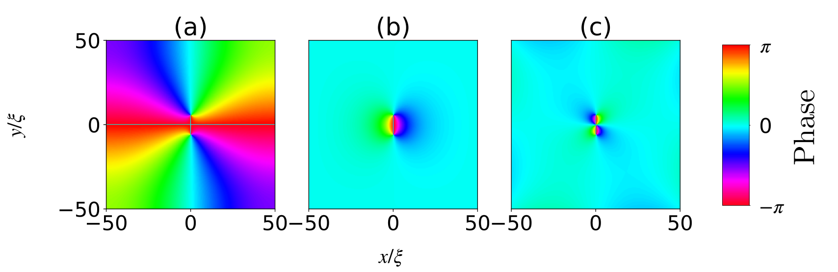
While Fig. 7 mostly supports our assumption that the twisted real projective plane boundaries efficiently remove boundary effects from the simulation, we also repeat the calculation of the vortex molecule energy in computational domains of different size. The results are shown in Fig. 8. We see that different box sizes broadly lead to the same energy as a function of molecular distance , but shifted by a constant value. This is expected as a larger computational domain will integrate a larger part of the energy density of the vortex flow pattern, which ultimately is expected to logarithmically diverge with increasing the box size. However, this does not matter for the purpose of Hamiltonian dynamics in the extended point-vortex model of Sec. III where a constant energy offset is irrelevant and does not change the resulting equations of motion. For the smaller box size of we can see some deviations from the otherwise parallel behavior of the data shown in Fig. 8, which we attribute to a boundary effect. It becomes prominent when the molecular separation is larger than half of the linear box dimension. Hence, we use the data with the largest box size for parametrizing the interaction energy.
A.2 Parameterization
For the purpose of the point vortex model it is very convenient to parameterize the interaction energy of a vortex molecule rather than relying on numerical data that is only available at specific discrete values of the molecular distance . We have performed calculations of the vortex molecule energy as a function of for altogether four different parameter values as shown in Fig. 9.
We fit the curves in Fig. 9 with two different functional forms depending on the value of . For we use
| (21) |
and for we use
| (22) |
where, are fitting parameters. The equilibrium distance of the vortex molecule is defined as . This is the molecular distance of the lowest energy configuration. We set , which ensures that has a minimum at . The relevant parameters for both cases are given in Table 2 & 2, where is the healing length and .
| 2 | 14.83 | 53.8687 | 0.0614 | 22.3328 |
|---|---|---|---|---|
| 2 | 8.83 | 26.9334 | 0.2824 | 25.1213 |
| c | |||||
|---|---|---|---|---|---|
| 2 | 1.0227 | 17.81416077 | -0.96324 | 17.81416075 | 33.3192 |
| 2 | 1.1218 | 10.0701960 | -0.8672 | 10.0701959 | 33.3336 |
This parametrization gives us a form for the interaction energy between the vortex molecules which we use to predict vortex trajectories along with our analytical model.
References
- Thouless (1998) David Thouless, Topological Quantum Numbers In Nonrelativistic Physics (World Scientific, 1998).
- Manton and Sutcliffe (2004) Nicholas Manton and Paul Sutcliffe, Topological Solitons (Cambridge University Press, Cambridge, 2004).
- García-Ripoll et al. (2002) Juan J. García-Ripoll, Víctor M. Pérez-García, and Fernando Sols, “Split vortices in optically coupled bose-einstein condensates,” Phys. Rev. A 66, 021602(R) (2002).
- Kasamatsu et al. (2004) Kenichi Kasamatsu, Makoto Tsubota, and Masahito Ueda, “Vortex Molecules in Coherently Coupled Two-Component Bose-Einstein Condensates,” Phys. Rev. Lett. 93, 250406 (2004).
- Nicklas et al. (2015) E. Nicklas, W. Muessel, H. Strobel, P. G. Kevrekidis, and M. K. Oberthaler, “Nonlinear dressed states at the miscibility-immiscibility threshold,” Phys. Rev. A 92, 053614 (2015).
- Farolfi et al. (2021a) A. Farolfi, A. Zenesini, D. Trypogeorgos, C. Mordini, A. Gallemí, A. Roy, A. Recati, G. Lamporesi, and G. Ferrari, “Quantum-torque-induced breaking of magnetic interfaces in ultracold gases,” Nat. Phys. (2021a), 10.1038/s41567-021-01369-y.
- Farolfi et al. (2021b) A. Farolfi, A. Zenesini, R. Cominotti, D. Trypogeorgos, A. Recati, G. Lamporesi, and G. Ferrari, “Manipulation of an elongated internal Josephson junction of bosonic atoms,” Phys. Rev. A 104, 023326 (2021b), arXiv:2101.12643 .
- Son and Stephanov (2002) D. T. Son and M. A. Stephanov, “Domain walls of relative phase in two-component bose-einstein condensates,” Phys. Rev. A 65, 063621 (2002).
- Eto et al. (2020) Minoru Eto, Kazuki Ikeno, and Muneto Nitta, “Collision dynamics and reactions of fractional vortex molecules in coherently coupled Bose-Einstein condensates,” Phys. Rev. Research 2, 033373 (2020).
- Cipriani and Nitta (2013) Mattia Cipriani and Muneto Nitta, “Crossover between Integer and Fractional Vortex Lattices in Coherently Coupled Two-Component Bose-Einstein Condensates,” Phys. Rev. Lett. 111, 170401 (2013).
- Tylutki et al. (2016) Marek Tylutki, Lev P. Pitaevskii, Alessio Recati, and Sandro Stringari, “Confinement and precession of vortex pairs in coherently coupled Bose-Einstein condensates,” Phys. Rev. A 93, 043623 (2016).
- Kasamatsu et al. (2016) Kenichi Kasamatsu, Minoru Eto, and Muneto Nitta, “Short-range intervortex interaction and interacting dynamics of half-quantized vortices in two-component Bose-Einstein condensates,” Phys. Rev. A 93, 013615 (2016).
- Calderaro et al. (2017) Luca Calderaro, Alexander L. Fetter, Pietro Massignan, and Peter Wittek, “Vortex dynamics in coherently coupled Bose-Einstein condensates,” Phys. Rev. A 95, 023605 (2017).
- Eto and Nitta (2018) Minoru Eto and Muneto Nitta, “Confinement of half-quantized vortices in coherently coupled Bose-Einstein condensates: Simulating quark confinement in a QCD-like theory,” Phys. Rev. A 97, 023613 (2018).
- Ketterle and Zwierlein (2008) Wolfgang Ketterle and Martin W Zwierlein, “Making, probing and understanding ultracold Fermi gases,” Riv. Nuovo Cimento 31, 247 (2008), arXiv:0801.2500 .
- Pethick and Smith (2008) C. J. Pethick and H. Smith, Bose-Einstein Condensation in Dilute Gases (Cambridge University Press, Cambridge, UK, 2008).
- Becker et al. (2013) C. Becker, K. Sengstock, P. Schmelcher, P. G. Kevrekidis, and R Carretero-González, “Inelastic collisions of solitary waves in anisotropic Bose–Einstein condensates: Sling-shot events and expanding collision bubbles,” New J. Phys. 15, 113028 (2013), arXiv:1308.2994 .
- Muñoz Mateo and Brand (2015) A. Muñoz Mateo and J. Brand, “Stability and dispersion relations of three-dimensional solitary waves in trapped Bose-Einstein condensates,” New J. Phys. 17, 125013 (2015), arXiv:1510.01465 .
- Brand and Reinhardt (2001) Joachim Brand and William P Reinhardt, “Generating ring currents, solitons and svortices by stirring a Bose-Einstein condensate in a toroidal trap,” J. Phys. B At. Mol. Opt. Phys. 34, L113–L119 (2001).
- Brand and Reinhardt (2002) Joachim Brand and William P. Reinhardt, “Solitonic vortices and the fundamental modes of the "snake instability": Possibility of observation in the gaseous Bose-Einstein condensate,” Phys. Rev. A 65, 043612 (2002).
- Komineas and Papanicolaou (2003) S. Komineas and N. Papanicolaou, “Solitons, solitonic vortices, and vortex rings in a confined Bose-Einstein condensate,” Phys. Rev. A 68, 043617 (2003).
- Yefsah et al. (2013) Tarik Yefsah, Ariel T Sommer, Mark J H Ku, Lawrence W. Cheuk, Wenjie Ji, Waseem S Bakr, and Martin W Zwierlein, “Heavy solitons in a fermionic superfluid.” Nature 499, 426–30 (2013), arXiv:1302.4736 .
- Ku et al. (2014) Mark J. H. Ku, Wenjie Ji, Biswaroop Mukherjee, Elmer Guardado-Sanchez, Lawrence W Cheuk, Tarik Yefsah, and Martin W Zwierlein, “Motion of a Solitonic Vortex in the BEC-BCS Crossover,” Phys. Rev. Lett. 113, 065301 (2014), arXiv:1402.7052 .
- Donadello et al. (2014) Simone Donadello, Simone Serafini, Marek Tylutki, Lev P Pitaevskii, Franco Dalfovo, Giacomo Lamporesi, and Gabriele Ferrari, “Observation of Solitonic Vortices in Bose-Einstein Condensates,” Phys. Rev. Lett. 113, 065302 (2014), arXiv:1404.4237 .
- Toikka and Brand (2017) L. A. Toikka and J. Brand, “Asymptotically solvable model for a solitonic vortex in a compressible superfluid,” New J. Phys. 19, 023029 (2017), arXiv:1608.08701 .
- Chomaz et al. (2015) Lauriane Chomaz, Laura Corman, Tom Bienaimé, Rémi Desbuquois, Christof Weitenberg, Sylvain Nascimbène, Jérôme Beugnon, and Jean Dalibard, “Emergence of coherence via transverse condensation in a uniform quasi-two-dimensional Bose gas,” Nat. Commun. 6, 6162 (2015), arXiv:1411.3577 .
- Kwon et al. (2021) W. J. Kwon, G. Del Pace, K. Xhani, L. Galantucci, A. Muzi Falconi, M. Inguscio, F. Scazza, and G. Roati, “Sound emission and annihilations in a programmable quantum vortex collider,” Nature 600, 64–69 (2021).
- Fialko et al. (2015) O. Fialko, B. Opanchuk, A. I. Sidorov, P. D. Drummond, and J. Brand, “Fate of the false vacuum: Towards realization with ultra-cold atoms,” EPL Europhys. Lett. 110, 56001 (2015), arXiv:1408.1163v2 .
- Schweigler et al. (2017) Thomas Schweigler, Valentin Kasper, Sebastian Erne, Igor Mazets, Bernhard Rauer, Federica Cataldini, Tim Langen, Thomas Gasenzer, Jürgen Berges, and Jörg Schmiedmayer, “Experimental characterization of a quantum many-body system via higher-order correlations,” Nature 545, 323–326 (2017).
- Brand et al. (2010) Joachim Brand, T. J. Haigh, and Ulrich Zülicke, “Sign of coupling in barrier-separated Bose-Einstein condensates and stability of double-ring systems,” Phys. Rev. A 81, 025602 (2010), arXiv:0805.4447 .
- Matthews et al. (1999) M. R. Matthews, B. P. Anderson, P. C. Haljan, D. S. Hall, C. E. Wieman, and E. A. Cornell, “Vortices in a Bose-Einstein Condensate,” Phys. Rev. Lett. 83, 2498–2501 (1999).
- Pérez-García and García-Ripoll (2000) Víctor M. Pérez-García and Juan J. García-Ripoll, “Two-mode theory of vortex stability in multicomponent bose-einstein condensates,” Phys. Rev. A 62, 033601 (2000).
- Jezek et al. (2001) D. M. Jezek, P. Capuzzi, and H. M. Cataldo, “Structure of vortices in two-component bose-einstein condensates,” Phys. Rev. A 64, 023605 (2001).
- Chui et al. (2001) S. T. Chui, V. N. Ryzhov, and E. E. Tareyeva, “Vortex states in a binary mixture of bose-einstein condensates,” Phys. Rev. A 63, 023605 (2001).
- Gallemí et al. (2018) A. Gallemí, L. P. Pitaevskii, S. Stringari, and A. Recati, “Magnetic defects in an imbalanced mixture of two bose-einstein condensates,” Phys. Rev. A 97, 063615 (2018).
- Pitaevskii and Stringari (2016) Lev Pitaevskii and Sandro Stringari, Bose-Einstein Condensation and Superfluidity (Oxford University Press, 2016).
- Kaurov and Kuklov (2005) V. M. Kaurov and A. B. Kuklov, “Josephson vortex between two atomic bose-einstein condensates,” Phys. Rev. A 71, 011601(R) (2005).
- Kaurov and Kuklov (2006) V. M. Kaurov and A. B. Kuklov, “Atomic josephson vortices,” Phys. Rev. A 73, 013627 (2006).
- Shamailov and Brand (2018) Sophie S. Shamailov and Joachim Brand, “Quasiparticles of widely tuneable inertial mass: The dispersion relation of atomic Josephson vortices and related solitary waves,” SciPost Phys. 4, 018 (2018), arXiv:1709.00403 .
- Kamchatnov and Pitaevskii (2008) A. M. Kamchatnov and L. P. Pitaevskii, “Stabilization of solitons generated by a supersonic flow of bose-einstein condensate past an obstacle,” Phys. Rev. Lett. 100, 160402 (2008).
- Gallemí et al. (2019) A. Gallemí, L. P. Pitaevskii, S. Stringari, and A. Recati, “Decay of the relative phase domain wall into confined vortex pairs: The case of a coherently coupled bosonic mixture,” Phys. Rev. A 100, 023607 (2019), arXiv:1906.06237 .
- Ihara and Kasamatsu (2019) Kousuke Ihara and Kenichi Kasamatsu, “Transverse instability and disintegration of a domain wall of a relative phase in coherently coupled two-component Bose-Einstein condensates,” Phys. Rev. A 100, 013630 (2019), arXiv:1904.02380 .
- Muryshev et al. (1999) A. E. Muryshev, H. B. van Linden van den Heuvell, and G. V. Shlyapnikov, “Stability of standing matter waves in a trap,” Phys. Rev. A 60, R2665–R2668 (1999).
- Bradley (2022) A. S. Bradley, “Vortexdistributions.jl,” (2022).
- Newton (2001) Paul K. Newton, The N-Vortex Problem, Vol. 145 (Springer New York, New York, NY, 2001) arXiv:1011.1669v3 .
- SI (2022) “Supplementary information,” (2022).
- Parker et al. (2004) N. G. Parker, N. P. Proukakis, C. F. Barenghi, and C. S. Adams, “Controlled Vortex-Sound Interactions in Atomic Bose-Einstein Condensates,” Phys. Rev. Lett. 92, 160403 (2004).
- Richaud et al. (2020) Andrea Richaud, Vittorio Penna, Ricardo Mayol, and Montserrat Guilleumas, “Vortices with massive cores in a binary mixture of bose-einstein condensates,” Phys. Rev. A 101, 013630 (2020).
- Richaud et al. (2021) Andrea Richaud, Vittorio Penna, and Alexander L. Fetter, “Dynamics of massive point vortices in a binary mixture of bose-einstein condensates,” Phys. Rev. A 103, 023311 (2021).