A search for transit timing variations in the HATS-18 planetary systemThanks: Based on data collected by MiNDSTEp with the Danish 1.54 m telescope at the ESO La Silla Observatory.
Abstract
HATS-18 b is a transiting planet with a large mass and a short orbital period, and is one of the best candidates for the detection of orbital decay induced by tidal effects. We present extensive photometry of HATS-18 from which we measure 27 times of mid-transit. Two further transit times were measured from data from the Transiting Exoplanet Survey Satellite (TESS) and three more taken from the literature. The transit timings were fitted with linear and quadratic ephemerides and an upper limit on orbital decay was determined. This corresponds to a lower limit on the modified stellar tidal quality factor of . This is at the cusp of constraining the presence of enhanced tidal dissipation due to internal gravity waves. We also refine the measured physical properties of the HATS-18 system, place upper limits on the masses of third bodies, and compare the relative performance of TESS and the 1.54 m Danish Telescope in measuring transit times for this system.
Keywords:
planetary systems — stars: fundamental parameters — stars: individual: HATS-181 Introduction
The hot Jupiters are a class of extrasolar planet characterised by a relatively large mass and a short orbital period. As a result, they are expected to undergo strong tidal interactions with their host stars (Ogilvie 2014; Mathis 2019, e.g.). This will lead to exchanges of angular momentum and energy between the stellar rotation and the planetary orbit. Since the host stars of most hot Jupiters have a rotational frequency below that of their planet’s orbital frequency, one manifestation of this interaction is orbital decay: a decrease in the orbital period of the planet and therefore the progressively earlier occurrence of transits in a system. Hence, observations of transit times can constrain the efficiency of such tidal interactions (Birkby et al. 2014; Maciejewski et al. 2018; Patra et al. 2020, e.g.). This in turn is relevant as a window on stellar structure (Love 1911) and on the ultimate fate of short-period planets (Levrard et al. 2009; Jackson et al. 2009; Matsumura et al. 2010).
It is therefore helpful to search for transit time variations (TTVs) in systems containing hot Jupiters. Because the effects of tides are small on a human timescale, it is wise to concentrate this search on the most promising systems. Maciejewski et al. 2018 used a result from Goldreich & Soter 1966 to develop an equation giving the expected shift in transit times as a function of the orbital period and mass ratio of a system plus the tidal efficiency and size of the host star (their eq. 2). We used this approach to rank all transiting extrasolar planets (TEPs) in TEPCat11 1 The Transiting Extrasolar Planet Catalogue (Southworth 2011) is at: https://www.astro.keele.ac.uk/jkt/tepcat/ in decreasing order of predicted transit shift over a ten-year period. The planetary system HATS-18 was found to be one of the best candidates, so we embarked on a campaign to determine precise transit times for this system over a period of several years.
HATS-18 was observed in the course of the HATSouth transit survey (Bakos et al. 2013) and its detection and characterisation was announced by Penev et al. 2016. It consists of a solar-type star (1.0, 1.0) with a gas giant (2.0, 1.3) in an orbit with a very short period (0.838 d). The properties of the system were measured (Penev et al. 2016) based primarily on a single high-quality transit light curve, six high-precision radial velocity (RV) measurements, and predictions from the Yonsei-Yale theoretical stellar evolutionary models (Demarque et al. 2004). Penev et al. 2016 also presented a detailed analysis of the tidal characteristics of the system, highlighting its importance in constraining tidal theory.
There has been little subsequent (published) work on the nature of HATS-18. Patra et al. 2020 presented two times of minimum obtained using a 60 cm telescope which were consistent with a constant orbital period. The system has also been observed in two sectors by the NASA Transiting Exoplanet Survey Satellite (TESS; Ricker et al. 2015). We used both datasets in our own analysis in order to obtain the best constraints on the orbital evolution of HATS-18.
Since our work on HATS-18 began, several theoretical studies of tidal dissipation have highlighted the importance of internal gravity waves in hot Jupiter systems and selected HATS-18 as a promising candidate (Barker 2020; Ma & Fuller 2021). Internal gravity waves are likely to be the dominant tidal mechanism in slowly rotating solar-type main-sequence stars with radiative cores (Barker & Ogilvie 2010; Chernov et al. 2017; Barker 2020; Ma & Fuller 2021, e.g.). In particular, the star HATS-18 A is one in which tidally-excited gravity waves are marginally predicted to break in the stellar core, depending strongly on the age of the star. When wave breaking occurs, stellar tidal dissipation is predicted to be efficient and can cause planetary orbital decay on Myr timescales for planets with orbital periods of approximately one day (Barker & Ogilvie 2010, e.g.). Such orbital decay is potentially observable in HATS-18, thus supporting our aim to search for TTVs in this system.
It is important to remember that there are multiple possible causes of TTVs. Orbital decay has been confidently detected in only one system, WASP-12 (Hebb et al. 2009; Maciejewski et al. 2016; Patra et al. 2017; Maciejewski et al. 2018). WASP-4 is also known to have a decreasing orbital period (Bouma et al. 2019; Southworth et al. 2019) but the origin of this is not yet settled (Baluev et al. 2020; Bouma et al. 2020; Turner et al. 2022). TTVs can arise due to the light-time effect caused by long-period companions in a system, as has been found for TrES-5 (Maciejewski et al. 2021), WASP-148 (Maciejewski et al. 2020) and HAT-P-26 (von Essen et al. 2019). TTVs can also be caused by apsidal precession (Patra et al. 2017), starspots (Watson & Dhillon 2004; Oshagh et al. 2013), the Applegate mechanism (Applegate 1992; Watson & Marsh 2010) and gravitational perturbations in multi-planetary systems (Holman & Murray 2005; Agol et al. 2005; Rowe et al. 2014, e.g.). Some of these effects can also cause changes in the orbital inclination and/or transit duration.
2 Observations
2.1 Danish Telescope
| Date of first | Start time | End time | Filter | Airmass | Moon | Aperture radii | Scatter | ||||
|---|---|---|---|---|---|---|---|---|---|---|---|
| observation | (UT) | (UT) | (s) | (s) | illumination | (pixels) | (mmag) | ||||
| 2017/05/13 | 23:07 | 01:03 | 48 | 100–150 | 13 | 1.08 1.00 | 0.913 | 16 24 45 | 1 | 1.05 | |
| 2017/05/29 | 00:34 | 04:14 | 117 | 100 | 13 | 1.01 1.83 | 0.156 | 13 21 45 | 1 | 1.03 | |
| 2017/06/09 | 23:29 | 02:36 | 100 | 100 | 13 | 1.00 1.42 | 0.996 | 11 18 40 | 1 | 1.56 | |
| 2017/06/13 | 23:26 | 01:58 | 81 | 80–100 | 13 | 1.01 1.33 | 0.825 | 12 20 50 | 1 | 1.78 | |
| 2017/06/18 | 23:31 | 03:12 | 110 | 100 | 13 | 1.03 2.07 | 0.331 | 13 20 40 | 1 | 1.15 | |
| 2017/07/09 | 22:49 | 02:00 | 91 | 100 | 25 | 1.09 2.22 | 0.993 | 11 18 40 | 2 | 1.19 | |
| 2018/04/24 | 23:34 | 03:31 | 123 | 100 | 14 | 1.20 1.00 1.06 | 0.735 | 10 20 40 | 2 | 1.06 | |
| 2018/04/29 | 23:34 | 04:13 | 140 | 100 | 14 | 1.14 1.00 1.18 | 0.998 | 9 15 30 | 2 | 1.33 | |
| 2018/05/05 | 00:50 | 04:32 | 117 | 100 | 14 | 1.01 1.00 1.31 | 0.768 | 10 20 40 | 1 | 1.15 | |
| 2018/05/20 | 23:08 | 02:58 | 118 | 100 | 16 | 1.04 1.00 1.20 | 0.374 | 10 18 40 | 1 | 1.28 | |
| 2018/05/25 | 23:19 | 03:30 | 125 | 100 | 16 | 1.01 1.00 1.41 | 0.874 | 10 18 50 | 1 | 2.45 | |
| 2018/06/20 | 22:50 | 02:30 | 109 | 100 | 14 | 1.01 1.69 | 0.564 | 14 22 50 | 1 | 1.36 | |
| 2019/05/17 | 01:39 | 05:14 | 108 | 100 | 16 | 1.03 1.94 | 0.961 | 9 18 40 | 1 | 1.37 | |
| 2019/05/22 | 22:56 | 01:40 | 82 | 85–100 | 15 | 1.03 1.00 1.02 | 0.826 | 9 16 35 | 1 | 1.20 | |
| 2019/06/01 | 23:09 | 02:43 | 133 | 60–100 | 16 | 1.01 1.00 1.31 | 0.023 | 9 16 40 | 2 | 1.22 | |
| 2021/05/14 | 23:19 | 03:46 | 103 | 100 | 28 | 1.02 1.00 1.04 | 0.094 | 8 15 30 | 2 | 1.13 | |
| 2021/05/25 | 01:43 | 02:55 | 111 | 100 | 15 | 1.02 2.25 | 0.972 | 9 16 35 | 2 | 1.52 | |
| 2021/06/04 | 22:48 | 02:15 | 106 | 100 | 18 | 1.01 1.00 1.26 | 0.246 | 13 20 40 | 2 | 1.80 | |
| 2021/06/09 | 23:37 | 02:53 | 99 | 100 | 18 | 1.01 1.00 1.54 | 0.002 | 10 16 35 | 2 | 1.43 | |
| 2021/06/14 | 23:32 | 03:30 | 80 | 100 | 18 | 1.02 1.00 2.09 | 0.192 | 14 20 40 | 1 | 2.34 |

HATS-18 was observed in the 2017, 2018, 2019 and 2021 observing seasons using the Danish 1.54 m telescope and DFOSC imager at ESO La Silla. No observations were performed in 2020 due to the Covid-19 pandemic. In all cases a Cousins filter was used to maximise the photon rate for this relatively faint star (), the telescope was operated out of focus to improve the photometric precision (Southworth et al. 2009a; Southworth et al. 2009b). DFOSC has a field of view of 13.7′13.7′ at a plate scale of 0.39′′ per pixel, but the CCD was typically windowed down to 12′8′ to decrease the readout time. The autoguider was not used because of technical issues.
A total of 20 transits were observed and an observing log is given in Table 1. Of the 20 transits, 13 were good, five were affected by atmospheric cloud or haze (2017/05/13, 2017/06/13, 2018/05/25, 2018/06/20, 2021/06/14) and two suffered from technical problems (2017/06/09, 2019/05/22).
Data reduction was performed using the defot pipeline (Southworth et al. 2009a; Southworth et al. 2014), which in turn uses routines from the NASA astrolib library22 2 http://idlastro.gsfc.nasa.gov/ idl33 3 http://www.harrisgeospatial.com/SoftwareTechnology/ IDL.aspx implementation of the aper routine from daophot (Stetson 1987). Image motion was measured by cross-correlating each image with a reference image obtained near the midpoint of that observing sequence. The software apertures were placed by hand on the reference images and the radii of the aperture and sky annulus were chosen manually. No bias or flat-field calibrations were applied, as we found that these had little effect beyond increasing the scatter of the results. Cloud-affected data were rejected when they gave measurements that were unreliable.
Differential-magnitude light curves were constructed by optimising the weights of between two and five comparison stars simultaneously with a low-order polynomial fitted to the out-of-transit data (Table 1). We consistently found that the choices taken during data reduction (bias, flat-field, aperture size, comparison stars, reference image) had little effect on the shape of the transit in the light curve but could have a significant effect on the scatter. The data are plotted in Fig. 1. We have placed them on the BJD(TDB) timescale using routines from Eastman et al. 2010.
2.2 Jongen Telescope
Nine transits of HATS-18 were observed in the 2020 season using the Yves Jongen Telescope at Deep Sky Chile. This is a PlaneWave Corrected Dall-Kirkham telescope with an aperture of 430 mm, mounted on a L500 Plane Wave Mount, and equipped with a Moravian 4G CCD camera and EFW 4L-7 filter wheel. This setup has a field of view of 21.0′15.8′ at a plate scale of 0.63′′ per pixel. A Chroma imaging IR-UV filter was used, which has a high transmission between 370 and 700 nm.
The data reduction was performed using the Munipack44 4 https://munipack.physics.muni.cz/ software. This comprised standard calibrations and brightness measurement using aperture photometry. Differential-magnitude light curves were calculated versus five nearby comparison stars.
2.3 Transiting Exoplanet Survey Satellite
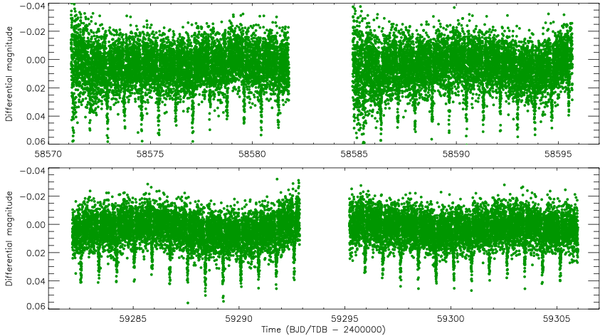
TESS (Ricker et al. 2015) observed HATS-18 in sectors 10 (2019/03/26 to 2019/04/22) and 36 (2021/03/07 to 2021/04/02). In both sectors it was selected as a short-cadence target. One further observation of HATS-18 with TESS is currently scheduled, in sector 69 (2023 March). We downloaded the available observations from the Mikulski Archive for Space Telescopes (MAST) archive55 5 https://mast.stsci.edu/portal/Mashup/Clients/Mast/ Portal.html and converted them into magnitude units.
We decided to use the pre-search data conditioning (PDCSAP) light curves (Jenkins et al. 2016) rather than the simple aperture photometry (SAP) observations, as they have a slightly lower scatter. We retained only those datapoints with a QUALITY flag of zero: 15 390 in sector 10 and 15 449 in sector 36. We further rejected all datapoints more than 0.24 d (three times the transit duration) from the mindpoint of a transit (approximately 71% of the data) as these were not useful for our analysis. The data are quite scattered due to the relative faintness of HATS-18, and the small aperture and large pixel scale of TESS (Fig. 2).
3 Physical properties of HATS-18
| Parameter | Symbol | Unit | This work | Penev et al. 2016 |
| Orbital period | d | |||
| Sum of the fractional radii | ||||
| Ratio of the radii | ||||
| Orbital inclination | ∘ | |||
| Fractional radius of star | ||||
| Fractional radius of planet | ||||
| Stellar effective temperature | K | |||
| Stellar metallicity | [Fe/H] | dex | ||
| Stellar velocity amplitude | m s-1 | |||
| Stellar mass | ||||
| Stellar radius | ||||
| Stellar surface gravity | (cgs) | |||
| Stellar density | ||||
| Planetary mass | ||||
| Planetary radius | ||||
| Planetary surface gravity | m s-2 | |||
| Planetary density | ||||
| Equilibrium temperature | K | |||
| Safronov number | ||||
| Semimajor axis | au | |||
| Age | Gyr |
The only existing measurement of the physical properties of the HATS-18 system is by Penev et al. 2016, who had access to only one high-quality transit light curve of the system. We have therefore redetermined the physical properties of HATS-18 using our extensive photometry and the methods from the Homogeneous Studies project (Southworth 2012, and references therein). The measured parameters are useful in subsequent analyses.
All modelling of the light curves of HATS-18 was done using version 42 of the jktebop66 6 jktebop is written in fortran77 and the source code is available at http://www.astro.keele.ac.uk/jkt/codes/jktebop.html code (Southworth 2013, and references therein). We first fitted each transit from the Danish Telescope individually, to check the level of scatter in the light curves. The fitted parameters were the transit midpoint (), the fractional radii of the two components ( and where is the radius of the star, is the radius of the planet, and is the semimajor axis of the relative orbit) expressed as their sum and ratio, and the orbital inclination ().
Once this was done, we merged the data from the 17 complete transits into a single light curve file, at the same time scaling the point errors in each dataset to obtain versus the best fit. We did not use the three partially-observed transits as they are less reliable than the others. We also did not use the transits observed with the Jongen telescope or TESS due to their higher scatter. We obtained a best model to the data by fitting for , , , , and a polynomial function for each transit (see Table 1). This was done for four different two-parameter limb darkening (LD) laws (Southworth 2008, see) and with either both coefficients fixed or the linear coefficient fitted. Fixed and initial values of the LD coefficients were taken from the theoretical tabulations by Claret 2000; Claret 2004b; Claret 2017.
The uncertainties in the fitted parameters were calculated using Monte Carlo and residual-permutation simulations (Southworth 2008, see). The adopted value of each fitted parameter is the weighted mean of the four fits with one LD coefficient fitted. Its uncertainty is the larger of the Monte Carlo and residual-permutation options, with an additional contribution from the variation in parameter values added in quadrature. These results are given in the top portion of Table 2.
To determine the physical properties of the system an additional constraint is needed (Southworth 2009) for which we resorted to interpolating within tabulated predictions of stellar properties from theoretical models. Measurements of the spectroscopic properties of the host star (temperature , metallicity [Fe/H], velocity amplitude ) were taken from Penev et al. 2016. We estimated an initial value of the velocity amplitude of the planet and used the measured values of , , , and to determine the physical properties of the system. This process was iterated to find the value of that gave the best match between the observed and predicted and . We included [Fe/H] as a constraint and performed a grid search over age to determine the overall best set of system properties. This process was undertaken for five different sets of theoretical stellar evolutionary models (Claret 2004a; Demarque et al. 2004; Pietrinferni et al. 2004; VandenBerg et al. 2006; Dotter et al. 2008).
Random errors were propagated using a perturbation approach and systematic errors were estimated from the differences between the five sets of solutions using the various theoretical predictions. Our final set of properties of the system are collected in Table 2, which also shows the values from Penev et al. 2016 for comparison. Our new observations have enabled, amongst other results, significantly better measurements of (a parameter important for tidal evolution) and (relevant in understanding the structure and evolution of planets). The age determination remains frustratingly uncertain; an improved value might be obtained from a more precise measurement. Although HATS-18 A has a measured rotation period of d (Penev et al. 2016) indicative of a relatively young age, there is evidence that gyrochronological ages are unreliable for the host stars of hot Jupiters (Poppenhaeger & Wolk 2014; Brown 2014; Maxted et al. 2015; Mancini et al. 2017).
4 Transit timing analysis
4.1 Measurement of the transit times
| BJD(TDB) | Cycle | Residual (s) | Source | |
|---|---|---|---|---|
| 2457410.80009 | 0.00030 | 1451.0 | 0.00024 | This work (Penev et al. 2016 transit) |
| 2457834.74845 | 0.00040 | 945.0 | 0.00037 | Patra et al. 2020 |
| 2457902.61444 | 0.00019 | 864.0 | 0.00027 | This work (Danish telescope) |
| 2457918.53333 | 0.00063 | 845.0 | 0.00013 | This work (Danish telescope) |
| 2457923.55998 | 0.00017 | 839.0 | 0.00028 | This work (Danish telescope) |
| 2457944.50658 | 0.00018 | 814.0 | 0.00022 | This work (Danish telescope) |
| 2458217.64370 | 0.00029 | 488.0 | 0.00026 | Patra et al. 2020 |
| 2458233.56286 | 0.00021 | 469.0 | 0.00038 | This work (Danish telescope) |
| 2458238.58946 | 0.00027 | 463.0 | 0.00008 | This work (Danish telescope) |
| 2458243.61625 | 0.00018 | 457.0 | 0.00035 | This work (Danish telescope) |
| 2458259.53486 | 0.00027 | 438.0 | 0.00077 | This work (Danish telescope) |
| 2458264.56344 | 0.00068 | 432.0 | 0.00074 | This work (Danish telescope) |
| 2458290.53560 | 0.00024 | 401.0 | 0.00025 | This work (Danish telescope) |
| 2458581.26804 | 0.00043 | 54.0 | 0.00038 | This work (TESS) |
| 2458620.64595 | 0.00021 | 7.0 | 0.00037 | This work (Danish telescope) |
| 2458626.51102 | 0.00045 | 0.0 | 0.00021 | This work (Danish telescope) |
| 2458636.56579 | 0.00020 | 12.0 | 0.00044 | This work (Danish telescope) |
| 2458898.81064 | 0.00036 | 325.0 | 0.00017 | This work (Jongen telescope) |
| 2458862.78435 | 0.00068 | 282.0 | 0.00117 | This work (Jongen telescope) |
| 2458883.72975 | 0.00048 | 307.0 | 0.00047 | This work (Jongen telescope) |
| 2458903.83713 | 0.00054 | 331.0 | 0.00040 | This work (Jongen telescope) |
| 2458950.75579 | 0.00088 | 387.0 | 0.00099 | This work (Jongen telescope) |
| 2458972.54162 | 0.00046 | 413.0 | 0.00090 | This work (Jongen telescope) |
| 2458982.59355 | 0.00078 | 425.0 | 0.00130 | This work (Jongen telescope) |
| 2459034.54221 | 0.00069 | 487.0 | 0.00105 | This work (Jongen telescope) |
| 2459292.59679 | 0.00029 | 795.0 | 0.00027 | This work (TESS) |
| 2459203.78668 | 0.00079 | 689.0 | 0.00107 | This work (Jongen telescope) |
| 2459349.57034 | 0.00020 | 863.0 | 0.00010 | This work (Danish telescope) |
| 2459359.62471 | 0.00021 | 875.0 | 0.00015 | This work (Danish telescope) |
| 2459370.51596 | 0.00040 | 888.0 | 0.00057 | This work (Danish telescope) |
| 2459375.54404 | 0.00042 | 894.0 | 0.00044 | This work (Danish telescope) |
| 2459380.57024 | 0.00058 | 900.0 | 0.00042 | This work (Danish telescope) |
We modelled the observed transit light curves individually as detailed in Section 3, fitting for , , , and the linear LD coefficient of the quadratic LD law. We also included a quadratic polynomial to model the out-of-eclipse brightness of the system, in order to capture the uncertainties in the light curve normalisation process at the data-reduction stage. The two transits from the Danish telescope lacking coverage of either the ingress or egress (2017/05/13 and 2017/06/09) were not included because such data do not give reliable transit times (Gibson et al. 2009, e.g.). Uncertainties on the transit times were obtained using Monte Carlo and residual-permutation simulations (Southworth 2008) and the larger of the two options was used. In cases where the reduced of the fit was the errorbar was further multiplied by to avoid underestimation of the uncertainties.
The TESS data demanded a different approach as the scatter is high. We therefore fitted all transits from each sector simultaneously to determine a single effective time of transit for that sector. The reference time of transit was chosen to be the observed transit closest to the midpoint of the data in each case, and a quadratic polynomial was included to account for slow drifts in the instrumental magnitudes of the system over the sector. The uncertainties were obtained using Monte Carlo simulations.
4.2 Published transit times
Penev et al. 2016 presented a single transit time, , from a joint analysis of all the light and radial velocity curves available to them. We did not wish to use this directly as it is measured from data taken over four years so is not suitable for any analysis where the orbital period may be changing. We therefore modelled the one follow-up light curve which has full coverage of a transit, using the same approach as above. This was taken on the night of 2016/01/22 using an LCOGT77 7 https://lco.global/ 1-m telescope and Sinistro imager at the Cerro Tololo Inter-American Observatory (CTIO88 8 https://noirlab.edu/public/programs/ctio/). The data were reported as BJD on the UTC time system so we converted the resulting transit time to TDB.
We subsequently found that this transit time occurred significantly later than expected (approximately 100 s) from a preliminary orbital ephemeris based on our Danish Telescope data. Dr. Joel Hartman kindly made available the original data for us to reduce using our own defot code. We found that our own light curve has timestamps in excellent agreement with those from Penev et al. 2016, even though ours are expressed in TDB and the published data are given in UTC. Furthermore, our own transit time is in much better agreement with the preliminary orbital ephemeris. We conclude that the timestamps from the published data are actually in TDB, not UTC. For subsequent analysis we therefore used our measurement of the transit time, from the light curve presented by Penev et al. 2016, under the assumption that the timestamps are in TDB.
Two further transit times of HATS-18 were given by Patra et al. 2020. These are already in BJD/TDB so were added to our analysis without modification. We are not aware of any further source of transit times for this system.
4.3 Orbital ephemerides

| Quantity | Linear ephemeris | Quadratic | Cubic |
|---|---|---|---|
| (adopted) | ephemeris | ephemeris | |
| Reference time (BJD/TDB) | 2458626.51123 (7) | 2458626.51120 (10) | 2458626.51129 (13) |
| Linear term (d) | 0.83784382 (11) | 0.83784382 (11) | 0.83784404 (22) |
| Quadratic term () | (0.61.7) | (1.22.3) | |
| Cubic term () | (2.92.5) | ||
| r.m.s. of residuals (s) | 50.2 | 50.2 | 49.5 |
| BIC | 64.2 | 67.5 | 68.7 |
| AIC | 61.3 | 63.1 | 62.9 |
Once the transit times were assembled we fitted them with a straight line to obtain a linear ephemeris:
where is the epoch of the transit and the bracketed quantities indicate the uncertainties in the preceding digits. The fit has , which is significantly larger than the 1.0 expected for a good fit but in line with our past experience that is usually more than 1.0 in this kind of analysis (Southworth et al. 2016; Baştürk et al. 2022, e.g.). The uncertainties in the ephemeris above have been multiplied by to account for this relatively poor fit. The transit times and their residuals are given in Table 3.
Once the linear ephemeris was established we tried fitting for quadratic and cubic ephemerides of the forms
and
where and are the coefficients of the quadratic and cubic terms, respectively. These give a very similar fit, with slightly larger values for the Bayesian Information Criterion (Schwarz 1978; Liddle 2007, BIC;) and Akaike Information Criterion (Akaike 1974, AIC;) than the linear ephemeris. The properties of these fits are compared with the linear ephemeris in Table 4 and shown graphically in Fig. 3. The uncertainties in the fitted coefficients were determined using 10 000 Monte Carlo simulations, which were found to be in excellent agreement with the formal errors outputted by the fitting code99 9 To fit the ephemerides we used the poly_fit routine in IDL..
The curvature term in the quadratic ephemeris represents a period decrease which could be attributed to tidally-induced orbital decay if it were negative. Instead it can be seen that this term is positive but consistent with zero. The cubic ephemeris is designed to allow the detection of a changing acceleration which could be attributed to orbital motion with a third body in the system. However, the quadratic and cubic ephemerides are not a significantly better fit to the data than the linear ephemeris, so we are only able to set upper limits on orbital period changes. Future monitoring of the system is needed to refine these limits and push the noise down below any real astrophysical signal.
Finally, we used the period04 package (Lenz & Breger 2005) to check for periodic variations in the residuals of the timings versus the linear ephemeris. No significant signals were found, with the strongest being at 0.0545 cycle-1 with a signal to noise ratio of 2.9, well below the commonly-used signal-to-noise ratio threshold of 4.0 (Breger et al. 1993). We therefore find no evidence in our data for a periodic variation in the times of transit for HATS-18.
4.4 Constraints on the tidal quality factor
The tidal quality factor, , is a measure of the efficiency of the dissipation of tidal energy (Ogilvie 2014, e.g.). To constrain we followed the approach from Birkby et al. 2014, which refers to the modified tidal quality factor
where is the Love number (Love 1911). This is related to measurable properties of the system via the equation
(Wilkins et al. 2017) where is simply , is the quadratic coefficient in the ephemeris, and the other terms have the meanings given in Table 2.
Our value of in Table 4 is greater than zero (i.e. it indicates an increasing orbital period) so would cause a negative if inserted blindly into the equation above. We therefore used its lower limit of to obtain the constraint that , where the errorbar comes from propagating the uncertainties in , and . This limit is comparable to previous constraints for other systems (Ogilvie & Lin 2007; Jackson et al. 2008; Penev et al. 2012, e.g.).
4.5 Comparison of the tidal quality factor with models for stellar tidal dissipation
HATS-18 is a 1.05 G-star and so it likely harbours a radiative core on the main sequence. It also rotates much slower than the planetary orbit: based on km s-1 (Penev et al. 2016), we obtain a lower bound on the stellar rotation period of approximately 8 d (Penev et al. 2016, cf. d in). Hence, the dominant tidal mechanism is expected to be excitation and dissipation of internal gravity waves launched from the radiative/convective interface into the radiative core (Goodman & Dickson 1998; Ogilvie & Lin 2007; Barker & Ogilvie 2010; Chernov et al. 2017; Barker 2020, e.g.). Hydrodynamical simulations show that if these waves have large enough amplitudes to break, they are efficiently damped (Barker & Ogilvie 2010; Barker 2011), so we may then estimate tidal dissipation rates by assuming these waves are completely absorbed. This gives a simple estimate for the stellar tidal quality factor (Barker 2020, see e.g. eq. 41 of), that can be computed using stellar models together with the currently observed planetary mass and orbital period (note: ).


The critical planetary mass required to cause wave breaking in the stellar core is predicted to be a strong function of stellar age (and mass). To explore this scenario, we computed the evolution of HATS-18 using mesa stellar models (Paxton et al. 2011; Paxton et al. 2013; Paxton et al. 2015; Paxton et al. 2018; Paxton et al. 2019, r12278, using an initial mass 1.05 and metallicity ;) and evaluated the critical planetary mass required to initiate wave breaking by applying eq. 47 in Barker 2020. Results for are shown in Fig. 4 (left panel) as a function of stellar age. This shows that wave breaking is not predicted for ages less than 3.5 Gyr, since exceeds the observed planetary mass (red dashed line). For ages older than 3.5 Gyr, wave breaking is expected in the stellar core, and we show the resulting prediction as a function of age in Fig. 4 (right panel). We typically find for ages less than approximately 3 Gyr (Barker 2020, similar to the predictions in). Since we have constrained , our prediction that is right at the limit of what can be tested by the available observations.
For earlier ages, or in general for cases where wave breaking is not predicted, gravity waves are likely to be much more weakly damped by radiative diffusion, with correspondingly much larger . Alternatively, weaker nonlinear effects such as parametric instabilities could be important, though tidal dissipation rates from these are hard to predict with certainty (Barker & Ogilvie 2011; Weinberg et al. 2012; Essick & Weinberg 2016, e.g.). On the other hand, if it is possible to enter the fully damped regime for gravity waves through processes other than wave breaking (as predicted above), theory would again predict . Such processes include gradual spin-up of the core due to radiative diffusion (Barker & Ogilvie 2010), and perhaps by wave breaking (for lower tidal amplitudes) initiated by passage through a resonance (e.g. Ma & Fuller 2021, since wave breaking would likely prohibit resonance locking). This system therefore remains a very interesting one for follow-up studies with further observations having a strong potential to test tidal theory.
4.6 Determining the upper mass limit of a hypothetical perturber
Having transit timing measurements gives an opportunity to place constraints on the upper mass limit of a hypothetical planetary companion. The amplitude of the timing residuals is directly proportional to the mass of the perturber for a given orbital distance. The root-mean-square (RMS) statistic of the timing residuals offers a reasonable estimate of the amplitude which enables an estimate of the upper mass limit of a putative perturbing body. Any TTV effect is amplified for orbital configurations involving mean-motion resonances (Agol et al. 2005; Holman & Murray 2005; Nesvorný & Morbidelli 2008) and should allow the detection of a low-mass planetary perturbing body. A larger perturbation implies a larger RMS scatter around the nominal ephemeris.
The applied method followed the technique described in Wang et al. 2017; Wang et al. 2018a; Wang et al. 2018b. The calculation of an upper mass limit was performed numerically via direct orbit integrations of the equations of motion. For this task, we modified the fortran-based microfarm1010 10 https://bitbucket.org/chdianthus/microfarm/src package (Goździewski 2003; Goździewski et al. 2008) which relies on OpenMPI1111 11 https://www.open-mpi.org to spawn several parallel tasks. The package’s main purpose is the numerical computation of the Mean Exponential Growth factor of Nearby Orbits (Cincotta & Simó 2000; Goździewski et al. 2001; Cincotta et al. 2003, MEGNO) over a grid of initial conditions of orbital parameters. In the present work we followed a direct brute-force method for the calculation of the RMS statistic.


We integrated the orbit of HATS-18 within the framework of the general three-body problem. The mid-transit time was calculated iteratively to a high precision from a series of back-and-forth integrations once a transit of HATS-18 b was detected. The best-fit radii of both the planet and the host star were accounted for. We then calculated an analytic least-squares regression to the time-series of transit numbers and mid-transit times to determine a best-fitting linear ephemeris with an associated RMS statistic for the TTVs. The RMS statistic was based on a twenty-year integration corresponding to 8711 transits by HATS-18 b. This procedure was then applied to a grid of masses and semimajor axes of the perturbing planet while fixing all the other orbital parameters. In this study, we chose to start the putative perturbing planet on a circular orbit that is coplanar with HATS-18 b. This implies that and for the perturber and for the transiting planet. This setting provides the most conservative estimate of the upper mass limit of a possible perturber (Bean 2009; Fukui et al. 2011; Hoyer et al. 2011; Hoyer et al. 2012). We refer the interested reader to Wang et al. 2018a, who studied the effects of TTVs on varying initial orbital parameters of the perturbing body.
In order to calculate the location of mean-motion resonances, we used the same code to calculate MEGNO on the same parameter grid. However, this time we integrated each initial grid point for 1000 years, which was found to be long enough to allow detection of the location of weak chaotic high-order mean-motion resonances.
Briefly, the MEGNO factor quantitatively measures the degree of stochastic behaviour of a nonlinear dynamical system and has proven useful in the detection of chaotic resonances (Goździewski et al. 2001; Hinse et al. 2010). In addition to the Newtonian equations of motion, the associated variational equations are solved simultaneously at each integration time step. The microfarm package implements the odex1212 12 https://www.unige.ch/~hairer/prog/nonstiff/odex.f extrapolation algorithm to numerically solve the system of first-order differential equations. This algorithm is slow but robust even for high-eccentricity orbits as well as close encounters. When presenting results (Fig. 5) we always plot the time-averaged MEGNO that is utilized to quantitatively differentiate between quasi-periodic and chaotic dynamics. We refer to Hinse et al. 2010 for a short review of the essential properties of MEGNO.
In a dynamical system that evolves quasi-periodically in time the quantity will asymptotically approach 2.0 for . In that case, the orbital elements associated with that orbit are often bounded. In the case of a chaotic time evolution the quantity diverges away from 2.0, with orbital parameters exhibiting erratic temporal excursions. For quasi-periodic orbits, we typically find to be less than 0.001 at the end of each integration.
Results are shown in Fig. 5 as MEGNO heat maps considering four different initial values in eccentricity for the putative perturbing planet. In each case, we find the usual instability region located in the proximity of the transiting planet (1:1 resonance) with MEGNO colour-coded as yellow (corresponding to ). The extent of these regions coincides with the results presented in Barnes & Greenberg 2006. The locations of mean-motion resonances are indicated by arrows in each map.
We find that a perturbing body (initial circular orbit) of upper mass limit of around 1– M⊕ will cause an RMS of the measured 52 s when located in the 2:1, 7:3, 5:2, 3:1 and 4:1 exterior resonance with HATS-18 b. For the 1:3 and 1:2 interior resonance, perturber upper mass limits of M⊕ and M⊕, respectively, could also cause an RMS mid-transit time scatter of 52 s. However, although we determined upper mass limits, in Section 4.3 we found no compelling evidence for any periodicities that can be attributed to an additional (non-transiting) planet within the HATS-18 system.
5 Summary and conclusions
HATS-18 consists of a massive planet (2) on a very short-period orbit (0.838 d) around a cool star (5600 K) with a convective envelope. It is a promising candidate for the detection of orbital decay due to tidal effects (Penev et al. 2016), particularly as it is at the cusp of experiencing enhanced tidal dissipation due to internal gravity waves (Barker 2020; Ma & Fuller 2021). We have obtained light curves of 20 transits from the 1.5 m Danish telescope and nine transits from the Jongen telescope. We measured 27 times of mid-transit from these data, plus two timings from the TESS light curves of HATS-18 in sectors 10 and 36. Together with three published measurements, this gives a total of 32 transit timings available for the system.
The transit timings were fitted with several ephemerides in three functional forms (linear, quadratic and cubic), with the finding that the linear ephemeris represents them best. This equates to a non-detection of orbital decay which can be used to put an upper limit on the tidal quality factor of the star, . This constraint is similar to our theoretical predictions in Section 4.5 if wave breaking occurs (or gravity waves are otherwise fully damped). This system therefore remains a very interesting one for follow-up studies with further observations having a strong potential to test tidal theory. One further sector of TESS data will (hopefully) become available in mid-2023, and additional ground-based timing measurements will help to strengthen the detection limit for orbital decay.
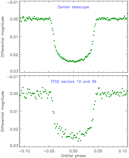
We have also obtained revised measurements of the physical properties of the HATS-18 system which are in agreement with and improve on previous results. This part of the analysis was based on the data from the Danish telescope only, due to the higher precision of the observations. This prompted us to make a comparison between the light curves from the Danish telescope and TESS. The Danish telescope has an aperture of diameter 154 cm and was used to observe 20 transits from the ground. TESS has an aperture of diameter 10.5 cm and observed 52 transits over two sectors from space. We normalised each transit to zero differential magnitude, converted them into orbital phase, and binned them into bins of duration 120 s. The results are shown in Fig. 6. It is clear that the ground-based observations are greatly superior to the space-based ones for a star of this relatively faint magnitude ( and ; Henden et al. 2012). This is due to the much larger aperture, which lowers photon noise, and finer pixel scale, which lowers noise from the sky background even when the telescope is operated out of focus.
Acknowledgements
We thank Dr. Kaloyan Penev and Dr. Joel Hartman for their help in tracking down the issue with the LCOGT transit timing.
AJB was supported by STFC grants ST/S000275/1 and ST/W000873/1. UGJ acknowledges funding from the Novo Nordisk Foundation Interdisciplinary Synergy Programme grant no. NNF19OC0057374 and from the European Union H2020-MSCA-ITN-2019 under Grant no. 860470 (CHAMELEON). PLP was partly funded by Programa de Iniciación en Investigación-Universidad de Antofagasta, INI-17-03. NP’s work was supported by Fundacaão para a Ciência e a Tecnologia (FCT) through the research grants UIDB/04434/2020 and UIDP/04434/2020. This research has received funding from the Europlanet 2024 Research Infrastructure (RI) programme. The Europlanet 2024 RI provides free access to the world’s largest collection of planetary simulation and analysis facilities, data services and tools, a ground-based observational network and programme of community support activities. Europlanet 2024 RI has received funding from the European Union’s Horizon 2020 research and innovation programme under grant agreement No. 871149. This research received financial support from the National Research Foundation (NRF; No. 2019R1I1A1A01059609).
The following internet-based resources were used in research for this paper: the ESO Digitized Sky Survey; the NASA Astrophysics Data System; the SIMBAD database operated at CDS, Strasbourg, France; and the ariv scientific paper preprint service operated by Cornell University.
Data availability
The light curves obtained with the Danish and Jongen telescopes will be made available at the Centre de Données astronomiques de Strasbourg (CDS) at http://cdsweb.u-strasbg.fr/. The TESS data used in this article are available in the MAST archive (https://mast.stsci.edu/portal/Mashup/Clients /Mast/Portal.html).
References
- Agol et al. (2005) Agol E., Steffen J., Sari R., Clarkson W., 2005, MNRAS, 359, 567
- Akaike (1974) Akaike H., 1974, IEEE Transactions on Automatic Control, 19, 716
- Applegate (1992) Applegate J. H., 1992, ApJ, 385, 621
- Baştürk et al. (2022) Baştürk Ö., et al., 2022, MNRAS, 512, 2062
- Bakos et al. (2013) Bakos G. Á., et al., 2013, PASP, 125, 154
- Baluev et al. (2020) Baluev R. V., et al., 2020, MNRAS, 496, L11
- Barker (2011) Barker A. J., 2011, MNRAS, 414, 1365
- Barker (2020) Barker A. J., 2020, MNRAS, 498, 2270
- Barker & Ogilvie (2010) Barker A. J., Ogilvie G. I., 2010, MNRAS, 404, 1849
- Barker & Ogilvie (2011) Barker A. J., Ogilvie G. I., 2011, MNRAS, 417, 745
- Barnes & Greenberg (2006) Barnes R., Greenberg R., 2006, ApJ, 647, L163
- Bean (2009) Bean J. L., 2009, A&A, 506, 369
- Birkby et al. (2014) Birkby J. L., et al., 2014, MNRAS, 440, 1470
- Bouma et al. (2019) Bouma L. G., et al., 2019, AJ, 157, 217
- Bouma et al. (2020) Bouma L. G., Winn J. N., Howard A. W., Howell S. B., Isaacson H., Knutson H., Matson R. A., 2020, ApJ, 893, L29
- Breger et al. (1993) Breger M., et al., 1993, A&A, 271, 482
- Brown (2014) Brown D. J. A., 2014, MNRAS, 442, 1844
- Chernov et al. (2017) Chernov S. V., Ivanov P. B., Papaloizou J. C. B., 2017, MNRAS, 470, 2054
- Cincotta & Simó (2000) Cincotta P. M., Simó C., 2000, A&AS, 147, 205
- Cincotta et al. (2003) Cincotta P. M., Giordano C. M., Simó C., 2003, Physica D Nonlinear Phenomena, 182, 151
- Claret (2000) Claret A., 2000, A&A, 363, 1081
- Claret (2004a) Claret A., 2004a, A&A, 424, 919
- Claret (2004b) Claret A., 2004b, A&A, 428, 1001
- Claret (2017) Claret A., 2017, A&A, 600, A30
- Demarque et al. (2004) Demarque P., Woo J.-H., Kim Y.-C., Yi S. K., 2004, ApJS, 155, 667
- Dotter et al. (2008) Dotter A., Chaboyer B., Jevremović D., Kostov V., Baron E., Ferguson J. W., 2008, ApJS, 178, 89
- Eastman et al. (2010) Eastman J., Siverd R., Gaudi B. S., 2010, PASP, 122, 935
- Essick & Weinberg (2016) Essick R., Weinberg N. N., 2016, ApJ, 816, 18
- Fukui et al. (2011) Fukui A., et al., 2011, PASJ, 63, 287
- Gibson et al. (2009) Gibson N. P., et al., 2009, ApJ, 700, 1078
- Goldreich & Soter (1966) Goldreich P., Soter S., 1966, Icarus, 5, 375
- Goodman & Dickson (1998) Goodman J., Dickson E. S., 1998, ApJ, 507, 938
- Goździewski (2003) Goździewski K., 2003, A&A, 398, 315
- Goździewski et al. (2001) Goździewski K., Bois E., Maciejewski A. J., Kiseleva-Eggleton L., 2001, A&A, 378, 569
- Goździewski et al. (2008) Goździewski K., Breiter S., Borczyk W., 2008, MNRAS, 383, 989
- Hebb et al. (2009) Hebb L., et al., 2009, ApJ, 693, 1920
- Henden et al. (2012) Henden A. A., Levine S. E., Terrell D., Smith T. C., Welch D., 2012, Journal of the American Association of Variable Star Observers, 40, 430
- Hinse et al. (2010) Hinse T. C., Christou A. A., Alvarellos J. L. A., Goździewski K., 2010, MNRAS, 404, 837
- Holman & Murray (2005) Holman M. J., Murray N. W., 2005, Science, 307, 1288
- Hoyer et al. (2011) Hoyer S., Rojo P., López-Morales M., Díaz R. F., Chambers J., Minniti D., 2011, ApJ, 733, 53
- Hoyer et al. (2012) Hoyer S., Rojo P., López-Morales M., 2012, ApJ, 748, 22
- Jackson et al. (2008) Jackson B., Greenberg R., Barnes R., 2008, ApJ, 678, 1396
- Jackson et al. (2009) Jackson B., Barnes R., Greenberg R., 2009, ApJ, 698, 1357
- Jenkins et al. (2016) Jenkins J. M., et al., 2016, in Proc. SPIE. p. 99133E
- Lenz & Breger (2005) Lenz P., Breger M., 2005, Communications in Asteroseismology, 146, 53
- Levrard et al. (2009) Levrard B., Winisdoerffer C., Chabrier G., 2009, ApJ, 692, L9
- Liddle (2007) Liddle A. R., 2007, MNRAS, 377, L74
- Love (1911) Love A. E. H., 1911, Some Problems of Geodynamics. Cambridge University Press, Cambridge, UK
- Ma & Fuller (2021) Ma L., Fuller J., 2021, ApJ, 918, 16
- Maciejewski et al. (2016) Maciejewski G., et al., 2016, A&A, 588, L6
- Maciejewski et al. (2018) Maciejewski G., et al., 2018, AcA, 68, 371
- Maciejewski et al. (2020) Maciejewski G., Fernández M., Sota A., García Segura A. J., 2020, AcA, 70, 203
- Maciejewski et al. (2021) Maciejewski G., Fernández M., Aceituno F., Ramos J. L., Dimitrov D., Donchev Z., Ohlert J., 2021, A&A, 656, A88
- Mancini et al. (2017) Mancini L., et al., 2017, MNRAS, 465, 843
- Mathis (2019) Mathis S., 2019, in EAS Publications Series, vol. 82. pp 5–33
- Matsumura et al. (2010) Matsumura S., Peale S. J., Rasio F. A., 2010, ApJ, 725, 1995
- Maxted et al. (2015) Maxted P. F. L., Serenelli A. M., Southworth J., 2015, A&A, 577, A90
- Nesvorný & Morbidelli (2008) Nesvorný D., Morbidelli A., 2008, ApJ, 688, 636
- Ogilvie (2014) Ogilvie G. I., 2014, ARA&A, 52, 171
- Ogilvie & Lin (2007) Ogilvie G. I., Lin D. N. C., 2007, ApJ, 661, 1180
- Oshagh et al. (2013) Oshagh M., Santos N. C., Boisse I., Boué G., Montalto M., Dumusque X., Haghighipour N., 2013, A&A, 556, A19
- Patra et al. (2017) Patra K. C., Winn J. N., Holman M. J., Yu L., Deming D., Dai F., 2017, AJ, 154, 4
- Patra et al. (2020) Patra K. C., et al., 2020, AJ, 159, 150
- Paxton et al. (2011) Paxton B., Bildsten L., Dotter A., Herwig F., Lesaffre P., Timmes F., 2011, ApJS, 192, 3
- Paxton et al. (2013) Paxton B., et al., 2013, ApJS, 208, 4
- Paxton et al. (2015) Paxton B., et al., 2015, ApJS, 220, 15
- Paxton et al. (2018) Paxton B., et al., 2018, ApJS, 234, 34
- Paxton et al. (2019) Paxton B., et al., 2019, ApJS, 243, 10
- Penev et al. (2012) Penev K., Jackson B., Spada F., Thom N., 2012, ApJ, 751, 96
- Penev et al. (2016) Penev K., et al., 2016, AJ, 152, 127
- Pietrinferni et al. (2004) Pietrinferni A., Cassisi S., Salaris M., Castelli F., 2004, ApJ, 612, 168
- Poppenhaeger & Wolk (2014) Poppenhaeger K., Wolk S. J., 2014, A&A, 565, L1
- Ricker et al. (2015) Ricker G. R., et al., 2015, Journal of Astronomical Telescopes, Instruments, and Systems, 1, 014003
- Rowe et al. (2014) Rowe J. F., et al., 2014, ApJ, 784, 45
- Schwarz (1978) Schwarz G., 1978, Annals of Statistics, 5, 461
- Southworth (2008) Southworth J., 2008, MNRAS, 386, 1644
- Southworth (2009) Southworth J., 2009, MNRAS, 394, 272
- Southworth (2011) Southworth J., 2011, MNRAS, 417, 2166
- Southworth (2012) Southworth J., 2012, MNRAS, 426, 1291
- Southworth (2013) Southworth J., 2013, A&A, 557, A119
- Southworth et al. (2009a) Southworth J., et al., 2009a, MNRAS, 396, 1023
- Southworth et al. (2009b) Southworth J., et al., 2009b, MNRAS, 399, 287
- Southworth et al. (2014) Southworth J., et al., 2014, MNRAS, 444, 776
- Southworth et al. (2016) Southworth J., et al., 2016, MNRAS, 457, 4205
- Southworth et al. (2019) Southworth J., et al., 2019, MNRAS, 490, 4230
- Stetson (1987) Stetson P. B., 1987, PASP, 99, 191
- Turner et al. (2022) Turner J. D., Flagg L., Ridden-Harper A., Jayawardhana R., 2022, AJ, 163, 281
- VandenBerg et al. (2006) VandenBerg D. A., Bergbusch P. A., Dowler P. D., 2006, ApJS, 162, 375
- Wang et al. (2017) Wang Y.-H., et al., 2017, AJ, 154, 49
- Wang et al. (2018a) Wang X.-Y., et al., 2018a, PASP, 130, 064401
- Wang et al. (2018b) Wang S., et al., 2018b, AJ, 156, 181
- Watson & Dhillon (2004) Watson C. A., Dhillon V. S., 2004, MNRAS, 351, 110
- Watson & Marsh (2010) Watson C. A., Marsh T. R., 2010, MNRAS, 405, 2037
- Weinberg et al. (2012) Weinberg N. N., Arras P., Quataert E., Burkart J., 2012, ApJ, 751, 136
- Wilkins et al. (2017) Wilkins A. N., Delrez L., Barker A. J., Deming D., Hamilton D., Gillon M., Jehin E., 2017, ApJ, 836, L24
- von Essen et al. (2019) von Essen C., et al., 2019, A&A, 628, A116