Direct detection of dark photon dark matter using radio telescopes
Abstract
Dark photons can be the ultralight dark matter candidate, interacting with Standard Model particles via kinetic mixing. We propose to search for ultralight dark photon dark matter (DPDM) through the local absorption at different radio telescopes. The local DPDM can induce harmonic oscillations of electrons inside the antenna of radio telescopes. It leads to a monochromatic radio signal and can be recorded by telescope receivers. Using the observation data from the FAST telescope, the upper limit on the kinetic mixing can already reach for DPDM oscillation frequencies at GHz, which is stronger than the cosmic microwave background constraint by about one order of magnitude. Furthermore, large-scale interferometric arrays like LOFAR and SKA1 telescopes can achieve extraordinary sensitivities for direct DPDM search from 10 MHz to 10 GHz.
Introduction– Ultralight bosons are attractive dark matter (DM) candidates, including QCD axions, axion-like particles, dark photons, etc. Essig:2013lka; Battaglieri:2017aum; ParticleDataGroup:2020ssz. Dark photon mixed with photon through a marginal operator at low energy is one of the simplest extensions beyond the Standard Model of particle physics Holdom:1985ag; Dienes:1996zr; Abel:2003ue; Abel:2006qt; Abel:2008ai; Goodsell:2009xc. It can be a force mediator in the dark sector Essig:2013lka; Fabbrichesi:2020wbt; Caputo:2021eaa or a DM candidate itself Redondo:2008ec; Nelson:2011sf; Arias:2012az; Graham:2015rva.
This work focuses on the dark photon dark matter (DPDM) with a mass, , comparable to the energy of radio frequency photons (20 kHz – 300 GHz). Ultralight DPDM can be produced through inflationary fluctuations Graham:2015rva; Ema:2019yrd; Kolb:2020fwh; Salehian:2020asa; Ahmed:2020fhc; Nakai:2020cfw; Nakayama:2020ikz; Kolb:2020fwh; Salehian:2020asa; Firouzjahi:2020whk; Bastero-Gil:2021wsf; Firouzjahi:2021lov; Sato:2022jya, parametric resonances Co:2018lka; Dror:2018pdh; Bastero-Gil:2018uel; Agrawal:2018vin; Co:2021rhi; Nakayama:2021avl, cosmic strings Long:2019lwl, and the non-minimal coupling enhanced misalignment Nelson:2011sf; Arias:2012az; AlonsoAlvarez:2019cgw with possible ghost instability Nakayama:2019rhg; Nakayama:2020rka. Radio-frequency DPDM can be constrained indirectly by Cosmic Microwave Background (CMB) spectrum distortion Arias:2012az; McDermott:2019lch; Arias:2012az; McDermott:2019lch; Caputo:2020bdy; Witte:2020rvb and directly by haloscope experiments like TOKYO Suzuki:2015vka; Suzuki:2015sza; Knirck:2018ojz; Tomita:2020usq, FUNK FUNKExperiment:2020ofv, DM pathfinder and Dark E-field Phipps:2019cqy; Godfrey:2021tvs, SHUKET Brun:2019kak, WISPDMX Nguyen:2019xuh, SQuAD Dixit:2020ymh, and recent experiments Cervantes:2022gtv; Ramanathan:2022egk; Cervantes:2022yzp; DOSUE-RR:2022ise. Axion haloscope search results Asztalos:2009yp; ADMX:2018gho; ADMX:2019uok; ADMX:2018ogs; HAYSTAC:2018rwy; HAYSTAC:2020kwv; Alesini:2020vny; Lee:2020cfj; Jeong:2020cwz; CAPP:2020utb; ADMX:2021nhd; Crisosto:2019fcj; Lee:2022mnc; Kim:2022hmg; Yi:2022fmn; Adair:2022rtw; HAYSTAC:2023cam; Quiskamp:2022pks; Alesini:2019ajt; Alesini:2022lnp; TASEH:2022vvu can be interpreted to DPDM limits Caputo:2021eaa; DPLimits, but some searches relying on the magnetic veto, e.g. RBF DePanfilis:1987dk and UF Hagmann:1990tj, cannot be translated into DPDM limits Gelmini:2020kcu; Caputo:2021eaa. Proposals and future experiments to search for DPDM include plasma haloscopes Lawson:2019brd; Gelmini:2020kcu, Dark E-field Godfrey:2021tvs, DM-Radio Parker:2013fxa; Chaudhuri:2014dla; 7750582; Chaudhuri:2018rqn, MADMAX Caldwell:2016dcw, and solar radio observations An:2020jmf; An:2023wij.
One category of broadband haloscope experiments uses a dish reflector to look for dark photons Horns:2012jf; Jaeckel:2013eha; Jaeckel:2015kea. The original proposal uses a spherical reflector to convert , and the monochromatic photons with energy are emitted perpendicular to the surface, thus focusing on the spherical center. This method has been applied to room-sized experiments Suzuki:2015vka; Suzuki:2015sza; Knirck:2018ojz; Tomita:2020usq; Godfrey:2021tvs; Brun:2019kak; FUNKExperiment:2020ofv, with variations using plane/parabolic reflectors or dipole antenna placed in a shielded room.
In this work, we propose to use existing and future radio telescopes to search for DPDM directly. With huge effective areas and great detectors, the sensitivities of large-scale radio telescopes can surpass current astrophysics bounds on radio-frequency DPDM by several orders of magnitude. We perform two types of studies: one exploits a single large dish antenna to convert dark photons into radio signals; the other uses antenna arrays forming interferometer pairs to receive radio signals, taking advantage of the long DPDM coherence.
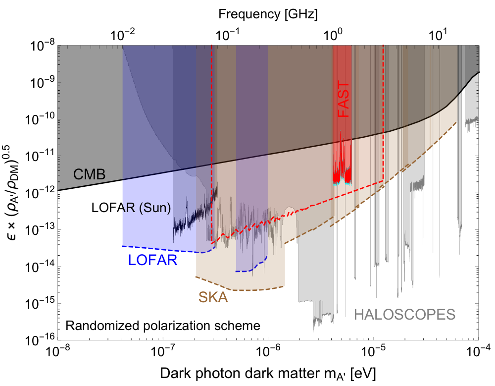
Fig. 1 summarizes our main results. The FAST data excludes the region surrounded by the solid red curve. The dashed red, blue, and brown curves show the projected sensitivities of FAST, LOFAR, and SKA1 footnote telescopes, assuming one-hour observation. For comparison, CMB and haloscopes constraints are shown by the black and gray shaded regions, respectively. The results show that large radio telescopes can play an essential and complementary role in DPDM searches.
Model– We consider the dark photon Lagrangian
| (1) |
and are dark photons and SM photons field strength; is the kinetic mixing. After appropriate rotation and redefinition, one can eliminate the kinetic mixing term and arrive at the interaction Lagrangian for , the SM photon , and the electromagnetic current ,
| (2) |
is the electromagnetic coupling. Therefore, free electrons in telescope antennas will be accelerated by the DPDM electric field, , and then produce EM equivalent signals.
Since the local DM velocity is about , where is the speed of light, oscillates with a nearly monochromatic frequency, . Therefore, radio telescopes will detect a monochromatic radio signal, broadening the center value of about . The DPDM wavelength is about , times the same-frequency EM wavelength. Next, we analyze DPDM signals for the dipole antenna, dish antenna, and antenna arrays.
Response of the dipole antenna– A dipole antenna usually comprises conductive elements like metal wires or rods. Considering a linear dipole antenna of length lying on the horizontal plane observing a radio signal from the zenith direction with frequency , it will detect an oscillating electric field
| (3) |
is the amplitude, is the wave number, and is the angle between the electric field and the antenna rod. is usually around half of the EM wavelength designed to detect. However, the DPDM wave number is about times smaller than due to the small DM velocity. Therefore, according to Eq. (2), the antenna will register an equivalent electric field,
| (4) |
is the amplitude of the dark electric field. is the angle between the dark electric field and the antenna rod.
Thus, typical dipole antennas respond to EM and DPDM fields differently, mainly by factors of and the polarization angle. Additionally, for the DPDM case, the antenna can always be seen as a short dipole antenna since for proposed frequencies, modifying the antenna efficiency by an number. Therefore, for general dipole antennas, one can define a DPDM-induced equivalent EM flux density,
| (5) |
is the conservative local DM energy density deSalas:2019pee; deSalas:2020hbh. is an numerical factor. For telescopes like LOFAR and SKA1-Low, detailed antenna designs are needed to simulate the exact values of , which is beyond the scope of the present work. Instead, we prove that for the antenna with linear dipole configuration, showing that the DPDM signal gains enhancement over the EM signal in Sec. II of the supplemental material (SUPP) chatterjee1996antenna. In this work, we conservatively assume to estimate the potential sensitivity of LOFAR and SKA1-Low.
Response of the dish antenna– Some large radio telescopes are constructed as dish antennas like FAST 2011IJMPD..20..989N or dish antenna arrays like MeerKAT 2016mks..confE….. and SKA1-Mid SKA1-MID-configuration. A dish antenna usually comprises a parabolic reflector with the feed receiving reflected EM wave at the focus. Dishes are commonly made of metal plates. According to Eq. (2), DPDM causes free electrons on metal plates to oscillate. Thus, each area unit can be seen as an oscillating dipole emitting EM waves with the same frequency as DPDM. Then, the feed signal is the integration over the dipole units. In Sec. I of SUPP, we show that the induced dipole with area is
| (6) |
is the projection of on . Then, the EM field at position can be obtained by summing up area units,
| (7) |
The electric field can be calculated using . EM phase at each dipole unit is determined by the DPDM wavelength, , different from the phase induced by parallel EM waves from distant stars. Therefore, the EM wave generated by DPDM will not focus on the antenna feed. For a single filled-aperture telescope like FAST, its diameter can be comparable to . Thus, numerical simulation is necessary to calculate the induced EM flux into the feed. However, for dish antenna arrays like MeerKAT and SKA1-Mid, each dish’s diameter is much smaller than . Therefore, each dish’s dipole units oscillate in phase.
Due to the continuous boundary condition for the electric field parallel to the metal surface, we have right outside the metal surface and the perpendicular component . In Sec. I of SUPP, detailed calculation shows that the reflected EM wave propagates nearly perpendicular to the surface of the metal plate. Right on top of the reflector surface, its energy density can be estimated as , where is the angle between and the reflector plate.
Since the DPDM-induced EM wave is not focusing, its flux into the feed is much smaller than the total reflected flux. The parabolic antenna feed size is usually around the EM wavelength to optimize the absorption, so the reduction factor is roughly, , the ratio between feed and reflector areas. Therefore, compared to the EM signal from distant sources, the DPDM-induced equivalent EM flux density can be written as
| (8) |
is an numerical factor determined by the detailed antenna design. Numerical calculations of are performed by averaging all possible polarization, denoted as the randomized polarization scheme.
Results for FAST and SKA1-Mid are shown in Sec. I.3 of SUPP.
Sensitivities of antenna arrays– Radio telescopes using radio interferometry techniques can effectively enlarge the effective area and get better sensitivities on faint signals. The basic observation unit for radio interferometer array is the antenna pair thompson2001. Let and be the signal measured by the -th and -th antenna, then up to amplification factors, the pair’s output signal is
| (9) |
means the time average. and can be seen as the voltage measured by antennas, proportional to the electric field. Therefore, the correlator is proportional to the EM flux density thompson2001. A telescope composed of antennas has independent pairs. The combined signal increases as , whereas the noise goes like . Thus, the signal-over-noise-ratio increases as .
For normal EM signals, the minimum detectable spectral flux density of a radio telescope is
| (10) |
is the number of polarizations, is the system efficiency, is the observation time, is the bandwidth, and SEFD is the system equivalent (spectral) flux density,
| (11) |
is the antenna system temperature. is the antenna array’s effective area, increasing with the number of antennas, .
For the DPDM-induced signal, the correlation length is determined by its wavelength, , beyond which the DPDM oscillation is out of phase; thus, the correlation is suppressed. For two antennas with distance , the correlation signal is suppressed by
| (12) |
is the most probable velocity in the Standard Halo Model McMillan:2009yr; Bovy:2009dr. The detailed derivation uses truncated Maxwellian distribution, as shown in Sec. III of SUPP Foster:2017hbq; OHare:2018trr; Evans:2018bqy; OHare:2019qxc; Foster:2020fln, consistent with Ref. Derevianko:2016vpm.
Therefore, for an antenna array composed of antennas, the DPDM-induced equivalent EM flux density is
| (13) |
where
| (14) |
is the suppression factor. is the DPDM-induced EM flux density for an individual antenna, given by (5) for dipole antenna and (8) for dish antenna. For dipole array telescopes like LOFAR and SKA1-Low, the antennas first form stations, which are further organized into a large interferometer. Since each station’s size is much smaller than , we neglect the suppression within a station. Therefore, the suppression factor becomes
| (15) |
is the number of stations. is the distance between the -th and -th stations.
Next, we will use the criterion
| (16) |
to estimate the projected sensitivities of LOFAR and SKA1 arrays for DPDM.
Constraints from FAST observation data– FAST is currently the largest filled-aperture radio telescope. Its designed total bandwidth is from 70 MHz to 3 GHz with the current frequency resolution kHz and designed sensitivity SEFD-1 = 2000 mK 2011IJMPD..20..989N; 2020Innov…100053Q. During observation, a 300-meter aperture instantaneous paraboloid is formed to reflect and focus the EM wave into the feed. The DPDM-induced EM wave is not focusing and therefore suffers from the suppression factor, ; see (8). The simulation of the factor for FAST at different frequencies is detailed in Sec. I.4 of SUPP, from which we can calculate the DPDM-induced EM spectral flux density detected by FAST,
| (17) |
Requiring , we can calculate the sensitivity for the FAST telescope.
Apart from the simulation, we use the 19-beam L-band (11.5 GHz) observation data from FAST to set upper limits for DPDM. The observation was conducted on December 14, 2020, lasting 110 minutes. A time series of the signal is recorded for each frequency bin. We use the noise diode temperature to calibrate data and convert the signal to the EM spectral flux density by pre-measured antenna gain. DPDM induces a time-independent line spectrum signal, whereas most noise sources have transient features and can be reduced by data filtering processes Foster:2022fxn. Our data filtering process is detailed in Sec. IV of SUPP Jiang:2019rnj; 2020RAA….20…64J; Foster:2022fxn; Cowan:2010js; Arias:2012az.
After data filtering, for each frequency bin, , we obtain the average measured spectral flux density, , and the statistic uncertainty, . We then use a polynomial function to locally model the background around the selected frequency bin with the help of its neighboring frequency bins. The systematic uncertainty is estimated by the data deviation to the background fit. Next, we assume a dark photon signal with the strength existing at bin , and a likelihood function can be built between data and background function with incorporated. Coefficients of the background polynomial function are treated as nuisance parameters. Following the likelihood-based statistical method Cowan:2010js, we compute the ratio between the conditional maximized-likelihood (e.g., only varying the nuisance parameters to maximize while keeping fixed) and the unconditional maximized-likelihood (e.g., varying both the nuisance parameters and to maximize ). Then the test statistic, , follows the half- distribution Cowan:2010js. Thus, we obtain the C.L. upper limit, , for a constant monochromatic signal, shown in Fig. 2.
Upper limits on the mixing parameter are obtained via . All 19 beams give similar constraints as expected. We choose the strongest limit among the 19 constraints for each frequency bin as the final result, shown in Fig. 1. The upper limits can reach in 11.5 GHz, about one order-of-magnitude better than the existing constraint from CMB measurement Arias:2012az.
We emphasize that every single frequency between 11.5 GHz is constrained by the real data without any extrapolation.
We also explore the rare case where the DPDM signal falls into two bins due to its broadening. The sensitivity calculation is similar but with a doubled data bandwidth.
More details about the FAST original data, filtering processing, statistical methods, and numerical calculations are given in Sec. IV of SUPP.
Sensitivities of LOFAR and SKA1– LOFAR is currently the largest radio telescope operating at the lowest frequencies ( MHz), containing low-band antennas (LBAs) and high-band antennas (HBAs). LOFAR antennas are grouped into 24 remote stations, each with a core size smaller than 2 kilometers. DPDM wavelength within the LOFAR frequency range is km. Therefore, we propose to use the core stations to search for DPDM. Station positions and relevant parameters can be found in Ref. vanHaarlem:2013dsa. The minimal frequency resolution, , of LOFAR is about 700 Hz vanHaarlem:2013dsa.
SKA1 continuously covers 50 MHz20 GHz, including SKA1-Low and SKA1-Mid telescopes. SKA1-Low has 131,072 dipole-like antennas grouped into 512 stations, covering 50350 MHz, with kHz. Station positions and relevant parameters can be found in Ref. SKA1-LOW-configuration; SKA1-Baseline-2. SKA1-Mid contains 133 SKA1 15-meter diameter and 64 MeerKAT 13.5-meter diameter dish-antennas. Therefore, its sensitivity on DPDM suffers from the additional suppression factor, ; see Eq. (8). SKA1-Mid has five bands, and the sensitivity and frequency range can be found in SKA1-Baseline-3 and dish locations in SKA1-MID-configuration. SKA1-Mid achieves Hz smaller than the DPDM natural width. Therefore, to calculate its DPDM sensitivity, we use the natural width, .
The suppression factor for DPDM signal using LOFAR and SKA1 arrays as interferometry are shown as the blue and red curves in Fig. 3, respectively. LOFAR is less suppressed than SKA1 due to lower frequency, thus longer DPDM coherent wavelength and smaller separation between stations.
Following Eq. (16), projected sensitivities on for LOFAR and SKA1 are shown in Fig. 1. LOFAR can cover a frequency down to 10 MHz, complementary to Haloscope searches.
SKA1 shows competitive sensitivity for higher frequencies as a broadband search compared to resonant cavity searches.

Summary and Outlook– The radio telescopes’ antennas can convert the DPDM field into an ordinary EM wave. We have analyzed the sensitivities of the commonly used dipole and parabolic dish antennas. We found that the parabolic one has a significant suppression factor for the DPDM-induced equivalent EM flux. For antenna arrays like LOFAR and SKA1, due to the sizeable coherent length of DPDM, the interferometry technique in radio astronomy can enhance the sensitivity.
We have used FAST observational data to set limits for DPDM. The result is encouraging that for 11.5 GHz, the limit is one order of magnitude stronger than the CMB constraint. We have projected the sensitivities for FAST, LOFAR, and SKA1 telescopes and found that compared to room-sized haloscope experiments, they are competing and complementary in searching for DPDM directly.
The DPDM can directly interact with electrons through (2), inducing a signal in the feed. As detailed in SUPP, the signal induced from the reflector studied in this work is about four times larger than the direct feed signal, due to geometric reasons. However, the feed shape is complex, making it difficult to calculate the direct contribution accurately. The interference between the reflector and feed, along with the direct signal, may result in an uncertainty for the FAST limits in Fig. 1. Furthermore, the FAST sensitivity could be significantly improved if one can raise the feed to higher locations as shown in SUPP.
Dark photon mass can be generated through the Higgs mechanism or the Stckelberg mechanism. For the Higgsed case, the sub-keV dark photon is constrained to by the stellar lifetime. is the dark U(1) gauge coupling. This assumes the dark Higgs has a dark charge of one and a mass below keV An:2013yua. Fig. 1 demonstrates that the proposed radio search complements the stellar constraint for small cases. For the Stckelberg case, the UV cutoff of dark photon model is constrained by the weak gravity conjecture Reece:2018zvv; Montero:2022jrc. Although some production mechanisms for radio DPDM, like inflation-induced DPDM Graham:2015rva, are no longer favored by certain constraints Reece:2018zvv, evading these constraints is possible by further developing the models Craig:2018yld. Therefore, a radio DPDM search could provide insights into DPDM production mechanisms.
Acknowledgements.
Acknowledgment– The authors would like to thank Peng Jiang, Yidong Xu, Jinglong Yu, Qiang Yuan and Yanxi Zhang for helpful discussions. This work made use of the data from FAST (Five-hundred-meter Aperture Spherical radio Telescope). FAST is a Chinese national mega-science facility, operated by National Astronomical Observatories, Chinese Academy of Sciences. The work of HA is supported in part by the National Key RD Program of China under Grant No. 2021YFC2203100 and 2017YFA0402204, the NSFC under Grant No. 11975134, and the Tsinghua University Initiative Scientific Research Program. The work of SG is supported by NSFC under Grant No. 12247147, the International Postdoctoral Exchange Fellowship Program, and the Boya Postdoctoral Fellowship of Peking University. The work of XH is supported by the Chinese Academy of Sciences, and the Program for Innovative Talents and Entrepreneur in Jiangsu. The work of JL is supported by NSFC under Grant No. 12075005, 12235001 and by Peking University under startup Grant No. 7101502458.Direct detection of dark photon dark matter using radio telescopes
In the Appendix, we show the detailed calculation for the response of the dish antennas. Additionally, we discuss the response of dipole antennas and provide proof that the response factor is larger than one. Thirdly, we derive the correlation factor of two distant antennas for the sensitivity calculation of dipole antenna array telescopes. Lastly, we provide a detailed analysis of FAST observational data, including data processing, background fit, and likelihood-based statistical tests.
I Response calculation for the dish antenna
The full Lagrangian for the kinetic mixing dark photon is
| (S1) |
By using variational principal, one obtains the Maxwell equations for the dark photon field,
| (S2) | ||||
| (S3) | ||||
| (S4) | ||||
| (S5) |
where and are the charge density and current density, and the elements of have been defined analogously to the electromagnetic field as
| (S6) | ||||
| (S7) |
The Maxwell equation for normal photon can be obtained as usual,
| (S8) | ||||
| (S9) | ||||
| (S10) | ||||
| (S11) |
In addition, one can determine the current in the conductor as,
| (S12) |
and the charge conservation is described as,
| (S13) |
I.1 Flat metal plate
First, we consider the situation of an infinitely large metal plate with thickness , which interacts with an incoming dark photon field. From Eqs. (S12), (S13) and Maxwell equations for and , we have:
| (S14) |
ignoring terms of order . From the Maxwell equations and Eq. (S12) one can derive:
| (S15) |
Similar equation holds for ,
| (S16) |
Assume the incoming dark photon takes the form of a plane wave,
| (S17) |
where the tilde means the field without plane wave factor and with a parameter ,
| (S18) |
the solution to Eq. (S14) is:
| (S19) |
Therefore, the charge density and current density are both of order , and from Eq. (S15) the electric field is also of order . Neglecting terms of order , Eq. (S16) can be simplified to
| (S20) |
which is the vacuum equation of . It implies that the dark electric field satisfies the same plane wave function inside the conductor.
Following Eqs. (S7) and (S17), the dark electric field can be written in an explicit form:
| (S21) |
Define another parameter
| (S22) |
the solution to Eq. (S15) is:
| (S23) |
where
| (S24) |

One can write more explicitly
| (S25) | ||||
| (S26) | ||||
| (S27) |
using the coordinate system shown in Fig. S1. The three equations above describe the electric field inside the conductor, . For , there is another plane wave going away from the conductor plate,
| (S28) |
where and can be determined by the boundary conditions and the dispersion relation of the photon,
| (S29) | ||||
| (S30) | ||||
| (S31) |
It is worth mentioning that the momentum of dark photons is much smaller than its rest mass, . Therefore, the wave vector is almost perpendicular to the conductor plate, with a tiny zenith angle of order .
Since the electromagnetic wave in the upper space is an ordinary plane wave solution to the Maxwell equations, the electric field is perpendicular to the wave vector. Together with the boundary conditions, can be obtained as
| (S32) | ||||
| (S33) | ||||
| (S34) |
If we ignore the velocity of the dark photon by taking , then we have:
| (S35) | ||||
| (S36) | ||||
| (S37) |
The normal magnetic field inside and outside the conductor can be derived accordingly, following the Maxwell equation (S10),
| (S38) | ||||
| (S39) | ||||
| (S40) | ||||
| (S41) | ||||
| (S42) | ||||
| (S43) |
Following the same procedure, one can obtain the field in the region. The only difference is an overall phase factor and a minus sign of the z-component of the wave vector. Defining the phase factor as
| (S44) |
the electromagnetic field below the plate can be expressed in terms of its counterpart in the upper space.
| (S45) | ||||
| (S46) | ||||
| (S47) | ||||
| (S48) | ||||
| (S49) | ||||
| (S50) |
Lastly, the current related to the plate can be obtained, which consists of three parts, the current density and the surface current on the upper surface and lower surface , respectively. The current density can be obtained by Eq. (S12),
| (S51) |
Considering a perfect conductor, e.g., aluminum, we can have , which implies . Therefore, the current density vanishes inside the conductor. It also implies is at the order of and cancels with the dark electric field as,
| (S52) |
For surface current, one can obtain their value on both sides of the metal plate using the boundary condition of the magnetic field,
| (S53) | ||||
| (S54) | ||||
| (S55) | ||||
| (S56) |
In summary, under the non-relativistic condition, good conductor, and thin plate assumptions, we arrive at the simplified results for the currents,
| (S57) | ||||
| (S58) | ||||
| (S59) |
Therefore, the flat metal plate behaves like an oscillating electric dipole , and its time derivative is
| (S60) |
where represents the projection of to the metal plane, and is the related surface area unit. We introduce two vectors and , representing the normal direction of the metal plate and the direction of respectively. Then the projection direction can be defined as,
| (S61) |
and .
I.2 DPDM-Induced EM flux
For the simulation of the response of the dish antenna to DPDM, the dish surface is divided into small pieces. The size of each piece is much smaller than the wavelength of the induced EM signal , but much larger than the thickness of the metal plate. Exploiting the results of dipole radiation, we obtain the induced EM field at position ,
| (S62) |
| (S63) |
It should be mentioned that for the FAST telescope, the DM velocity has a non-trivial contribution to the phase factor in the above equations because the telescope size is comparable to the wavelength of DPDM . Therefore, the time-averaged energy flux density of the induced EM wave can be written as
| (S64) |
The value of can be calculated from the local DM energy density. From the Lagrangian (S1), we obtain
| (S65) |
With Eqs. (S62), (S63), (S64), and (S65), the energy flux density can be calculated numerically.
For example, we can calculate the energy flux going into the feed analytically for a spherical metal plate with a radius where the feed is placed at the center. Assuming the size of the antenna is much smaller than the wavelength of dark photons, the energy flux density at the center is
| (S66) | ||||
where , . The angle describes how large is the spherical surface with for the surface shrinking to a point and for the surface becoming a full sphere. The describes the angles between the polarization vector of , , and the z-direction. The large ratio explicitly shows the enhancement from the ray optics focusing effect because the induced EM wave is perpendicular to the surface and is greatly enhanced for a spherical surface. For polarization in the z-direction, , the energy flux density will go to zero. For other , one can calculate the best , which has the largest energy flux density. This analytic formula helps people design the spherical mirror, which can help compromise efficiency and cost.
For the FAST telescope, the part of the dish that faces the feed deforms into a 300-meter diameter parabolic shape with the feed located at the focus. As a result, for the DPDM signal, we no longer have the enhancement factor .
At the end of this subsection, we demonstrate the difference between the parabolic mirror and spherical mirror by Fig. S2 drawing in the ray-optics schematic plots. The induced EM flux from parallel incident EM wave (orange) and DPDM (blue) are shown, where we assume the coming direction of the incident EM wave matches the parabolic mirror. At the same time, we do not need to specify the incoming direction of DPDM, because the induced EM waves are always perpendicular to the mirror’s surface. For the parabolic mirror, the parallel EM waves are focused in the focal point, while the DPDM-induced EM waves are spread into a focal volume. For the spherical mirror, the vice versa happens where DPDM induced EM wave focused in the spherical center. Therefore, there is an enhancement for parallel EM wave incident on the parabolic mirror, while for DPDM incident on the spherical mirror.
I.3 Calculation of the parameter for dish telescopes
Here we present the detailed calculation of the parameter, used in estimating the future reaches of the FAST and SKA1-Mid telescopes. The parameter is defined in Eq. (8) for dish telescopes to calculate the projections of their sensitivities. In Eq. (8), is defined as the equivalent flux density of a plane EM wave from infinite faraway that will produce the same signal strength as the DPDM. Therefore, to calculate , we also need to simulate the EM flux density at the position of the feed induced by the plane EM wave from an infinite faraway. The simulation is parallel to the DPDM signal simulation discussed above. The only difference is that the phase of the dipole oscillations in the metal plate of the reflector is now controlled by the plane EM wave, such that the reflected EM wave will focus on the feed position.
The feed size is usually designed to be around the wavelength to optimize the signal. Therefore, to estimate the sensitivity, we assume the feed of the future detectors to be a round shape with a diameter equal to . And both the DPDM-induced flux and EM plane wave-induced flux received by the feed are calculated as
| (S67) |
where is the flux along the direction of the receiver of the feed. As an illustration, the distributions of for both the EM and DPDM-induced signals at the feed are shown in Fig. S3 for the FAST telescope. We can see that for the EM-induced signal drops quickly when it is away from the center of the feed. However, for the DPDM-induced signal is almost flat. Then the explicit expression for can be written as
| (S68) |
where is the area parameter. For , is the energy density of the DPDM, and for , is the energy density of the parallel EM field. Since both the and are linear in , the dependence on is canceled, and therefore is independent of .
The values of for calculating the projective sensitivities of the FAST and SKA1-Mid telescopes are shown in Fig. S4. One can see that the values of are independent of in the high-frequency region. However, in the low-frequency region, when becomes larger than the size of the telescope, starts to show an oscillation pattern as shown by the red curve in Fig. S4. The reason is that when the wavelength of DPDM, , is significantly larger than the size of the telescope, the induced EM waves on the reflector plate share the same phase and form a stationary wave-like structure inside the reflector bowl. As a result, the positions of the nodes and antinodes change with the frequency, which causes the oscillation pattern of for FAST in the low frequency region.
I.4 The calculation of
The data we acquire from the FAST observation has been interpreted as the plane EM wave from distant stars. Therefore, to calculate the constraint, we first need to calculate . The current feed of the FAST telescope is composed of 19 beam receivers. The diameter for each beam receiver is cm. Therefore, when calculating in Eq. (S67), the upper limit of the radial integral needs to be replaced by , and the value of , in this case, depends on the frequency. We have simulated the values of at different frequencies, averaging over the dark photon velocity distribution and polarizations. The result is shown in Fig. S5. Then, the equivalent EM flux density induced by DPDM can be expressed as
| (S69) |
For example, using the simulated , we have at GHz with the area parameter plugged in. Later, we will compare the simulation result with the observation data of FAST and set limits on the kinetic mixing coupling .
The detector in the feed can also directly detect a signal generated by DPDM oscillation. However, accurately calculating this signal is difficult due to the complexity of the feed’s structure. To estimate the direct signal, we use the equivalent electric field method developed in this work. The equivalent electric field at the feed’s position can be expressed as:
| (S70) |
where the spatial phase is omitted since we have only one antenna. Then, we can estimate the equivalent flux detected by the feed as
| (S71) |
where the factor of accounts for the fact that the detector is designed to detect transverse polarized EM waves. By using the ratio , we can estimate the relative gain provided by the dish to the direct signal. This ratio is shown as a function of frequency in Fig. S6, where it can be seen that the relative gain is almost frequency-independent in the sensitive region of FAST. The different colors in the figure correspond to different heights of the feed. In the current observation, the feed is located at meters, and the relative gain is about four. This implies that the reflector-induced signal is about four times larger than the direct signal, which can be understood from the geometric picture shown in Fig. S2. Since the feed is located at the half-radius position of the focal surface, and the reflector-induced EM wave is perpendicular to the reflector surface, the energy flux of the reflector-induced EM wave at the focal surface is enhanced by roughly a factor of four due to energy conservation. This explains the four-fold relative gain between the dish-induced signal and the direct signal.
Furthermore, the sensitivity of FAST could be significantly improved by raising the feed to higher locations. The calculations indicate that by placing it at a distance of meters, the relative gain could increase by a factor of , as demonstrated in Fig. S6. Thus, it would be worthwhile to cooperate with the FAST team to determine if raising the feed is feasible within their mechanical system.
One may be concerned about interference between the direct and dish-induced signals. However, the feed is positioned approximately 140 meters above the reflector, resulting in significant suppression of the interference effect. Using Eq. (12), we can estimate the interference suppression factor to be approximately 0.3. Additionally, the size of the reflector will induce cancellations, further reducing the interference contribution. As a result, the interference contribution can be neglected compared to the direct signal. Furthermore, due to the complex nature of the feed structure, accurately simulating the direct and interference contributions is difficult. Therefore, in this study, we only use the reflector-induced signal to calculate the FAST constraint. In addition, the interference between reflector and feed, along with the direct signal may result in an uncertainty for the FAST limits.
II Response calculation of the dipole antenna
The LOFAR and SKA1-Low telescopes are composed of dipole antennas. The antennas are composed of metal bars with different lengths to achieve wideband observations. For example, the antennas of LOFAR LBA have two uneven dipole components, whereas SKA1-Low uses log-periodic dual-polarized antennas. Therefore, accurate calculations of the responses require complex antenna configurations, which is hard to get analytic results and physics intuition. One needs to do accurate numerical simulations of the fields and currents inside the antennas for both DPDM-induced and electromagnetic wave-induced signals. We will leave this for future studies when applying to the LOFAR and SKA1-Low observational data.
Instead, we take the commonly used linear dipole antenna as an example and work out the response factor for DPDM analytically. In general, the induced electric currents on the wire should be calculated, which has been done for distant parallel EM waves in textbook chatterjee1996antenna. We will show that the result for DPDM can be obtained smartly by comparing it to an incoming EM wave with . We prove that is exact for DPDM signals and explain its physics. As a result, we use to estimate the projections of the sensitivities for LOFAR and SKA1-Low. These sensitivities should be considered as conservative estimates.
The picture of an equal arm linear dipole antenna is shown in Fig. S7, where the wire is placed along the z-direction. The DPDM and EM waves propagate with an angle to the z-axis. Moreover, their polarizations are assumed to be the same. Since the DPDM wavelength , and given the fact that the length of linear antenna in the antenna design, the field variation is hard to see in the figure. Without loss of generality, the electric fields and are set to be in the y-z plane because the component in the x direction can not generate an electric current in the linear antenna.
For incoming EM and DPDM waves in Fig. S7, their electric fields on the wire can be described as,
| (S72) | ||||
| (S73) |
where we have taken the wire at , while and are their associate phases. The oscillation frequency is the same, , but the relation relates the wave number and . In the second equality of Eq. S73, we have used according to the fact that , with the EM wavelength .
First, we study the special case of the wave that comes from the y-direction, , which serves as a benchmark for calculation. In this case, we have . Therefore the electric fields for EM and DPDM are the same. Recall their coupling to currents, , it is clear that in this case.
Next, we consider general incidence, which has an important observation that the z-component of is
| (S74) |
It means that the effect of a DPDM wave from incident angle is the same as an EM wave incident from , with a suppression factor , because only the component can induce a current in the linear wire.
Therefore, to compare DPDM and EM waves both from angle, we need to compare the effects from EM waves for and . Fortunately, this is described by the far-field radiation pattern function chatterjee1996antenna as
| (S75) |
As a result, the response factor for DPDM incident from any is given by,
| (S76) |
In Fig. S8, we plot contours for , for and . The commonly used linear dipole antennas are the half-wavelength dipole antenna with and for the full-wavelength dipole antenna. For , the currents in the rod start to cancel each other. Thus, we focus on the region .
In Fig. S8, the results show that is exact for all directions and wavelengths. For , it is precisely equal to 1, as explained. It blows up in the corner of and because the full-wavelength dipole antenna is usually more directional.
The reason that the DPDM signal has feature can be understood in the following. For DPDM, since , the antenna wire always feels a uniform dark electric field. Therefore, the induced current is only weakened by the polarization projection. For the EM case, however, the antenna wire feels the spatial oscillation of the electric field, such that the electric field cancels with each other when driving the electric current in the wire. As a result, the EM-induced electric current is weaker than the DPDM signal. The cancellation argument can also work for complex experiment setups. Thus we expect that taking is conservative.
III Correlation of the antennas
The electric field induced by DPDM at each location can be expressed as,
| (S77) |
where is a random phase associated with the momentum and the energy is . We average the plane wave function using the truncated Maxwellian distribution (known as the Standard Halo Model), where is a normalization factor. We have and , where is most probable velocity and is the escape velocity McMillan:2009yr; Bovy:2009dr.
Next, we calculate the correlation of the field at the same location, which should return to its dark photon energy density,
| (S78) | ||||
| (S79) |
Due to the randomness, we assume there is no correlation between different phases, thus
| (S80) |
where is a dimensionful constant. Therefore, we can explicitly work out the energy density of dark photons as
| (S81) | ||||
with and is the error function. In the second line, we take the limit of large . The result shows that the energy density is uniform in time and space.
Similarly, we calculate the correlation of signals at different locations. The full formula using Standard Halo Model is given below,
| (S82) |
where . The full result can be simplified using Taylor expansion over the large or , which leads to the leading term and the next-to-leading term as
| (S83) |
It is clear that an exponential factor further suppresses the next-to-leading term compared with the leading term. Therefore, the leading term is already a good approximation in the numeric calculation. This result agrees with the equal-time two-point correlation function in Ref. Derevianko:2016vpm. Our method utilizes the random phase of each mode, which is equivalent to the specific Fock state in Ref. Derevianko:2016vpm.
The above results are derived based on the Standard Halo Model. However, there are possibilities for a non-standard halo model and non-trivial substructure like the streams S1/S2, which can significantly impact the signal Foster:2017hbq; OHare:2018trr; Evans:2018bqy; OHare:2019qxc. One aspect of the impact is the modification of the shape of the signal power spectral density, which can be noticed with high-frequency resolution measurements such as the axion resonant cavity searches. For the dark photon signal with radio telescope searches, the frequency resolutions for existing telescopes are kHz for FAST, Hz for LOFAR, while for future telescopes, are kHz for SKA1-Low and Hz for SKA1-Mid. Compared with their operating frequency ranges, only SKA1-Mid can have a chance to resolve the structure of signal power spectral density. Therefore, the current radio telescopes are challenging to discriminate different halo models.
Another aspect of the impact is the change in correlation patterns. Eq. (S77) should be implemented with the new velocity distribution function, thus modifying the form of the correlation . The network of detectors can reveal the correlation pattern and the directional information of the DM phase space distribution Foster:2020fln. While constructing additional detectors for axion experiments to form a network can be challenging, it is comparatively simple for antenna arrays in dark photon detection since each antenna has a straightforward structure that is easy to build. For example, LOFAR, which consists of 40 stations with multiple antennas inside each station, has already been built. Although increasing data storage and modifying data processing for local detection via radio telescopes present additional challenges, today’s technology provides the means to overcome these challenges.
IV Analysis of the FAST data
In this part, we present the detailed analysis of the FAST data to calculate the upper limit on the mixing parameter in the DPDM model.
The FAST observation was conducted between 2020-12-14 at 07:00:00 and 2020-12-14 at 08:50:00. The 19-beam receiver equipped on the FAST Jiang:2019rnj recorded data of two polarisations through 65536 spectral channels, covering the frequency range of GHz. The SPEC(W+N) backend was employed in the observation, with 1 second sampling time. The “ON/OFF” observation mode of the FAST was used for the original motivation, constraining the WIMP property by searching for synchrotron emission in the dwarf spheroidal galaxy Coma Berenices. In each round of observation, the central beam of the FAST was pointed to the Coma Berenices for 350 seconds, and the central beam of the FAST was moved to the “OFF source” position, which was a half degree away from the “ON source” without known radio sources, for another 350 seconds. There were nine rounds of ON/OFF observation. The low noise injection mode was used for signal calibration, with the characteristic noise temperature of about 1.1 K 2020RAA….20…64J. In the whole observation, the noise diode was continuously switched on and off for a period of 1 second.
Let be the original instrument reading without noise injection, be the reading with noise injected. Then the system temperature can be calibrated as 2020RAA….20…64J
| (S84) |
where is the pre-determined noise temperature measured with hot loads. from both polarizations were checked without large variation, and each pair of polarization temperatures was added to get the average. Then, the polarization-averaged was converted to flux density with pre-measured antenna gain, which is beam dependent 2020RAA….20…64J. With these procedures, the flux density for each beam, each time bin, and each frequency bin could be obtained. Finally, these flux densities in the time domain are checked, and time bins, when the telescope is not stable due to switching between ON and OFF, were masked, leaving 2232 time bins (1116 time bins for the ON observations and 1116 time bins for the OFF observations) for each frequency.
IV.1 Data processing
We are going to utilize the ON data. As mentioned above, each of the 19 beams covers the radio frequency range 11.5 GHz divided evenly into 65536 frequency bins (the bandwidth is ), and each frequency bin has 1116 time bins. The data suffer from large noise fluctuation [e.g., radio frequency interference (RFI)]. To reduce the effect of the noise fluctuation, we adopt the following method to clean the data (see e.g., Ref. Foster:2022fxn for a similar method but more complicated in their case).
The cleaning process is applied to the time series at each frequency bin. For each frequency bin , we divide the 1116 time bins consecutively into 33 groups, and thus each group contains 33 time bins (the last group contains 27 time bins). We identify the group with the smallest variance, , as the reference group. The mean value of the reference group is labeled as . We then regroup the time series by keeping only the bins with deviation from the reference group smaller than (i.e., ).
After the above cleaning process, the number of the remaining time bins in the time series reduces to with the mean ,
| (S85) |
where and label the frequency and time, respectively. The standard deviation of the mean (called the standard error, ) is thus
| (S86) |
which can be used as statistical uncertainty. As an example, in Fig. S9, we present the time series before (yellowblue) and after (yellow) cleaning for the frequency bin () of beam 1. For each beam, we apply the cleaning process and calculate and for all the 65536 frequency bins. The filtered time-average brightness distribution as a function of frequency is shown by the yellow curve in Fig. S10, compared with the time-average brightness without data cleaning (blue curve).

IV.2 Background fit
We fit the background around the frequency bin with a polynomial function
| (S87) |
It describes the observed data locally from the frequency bin to the bin . In practice, we choose and .
The systematic uncertainty due to the background fit can be estimated as follows. We first use the method of weighted least squares to fit the background by minimizing the function
| (S88) |
The result is labeled as so that the background minimizes (S88). Then the systematic uncertainty on bin can be estimated by the deviation of the data to the fitted background curve defined as
| (S89) | ||||
where
| (S90) |
We then add the statistical uncertainty and systematic uncertainty in quadrature form as the total uncertainty of the frequency bin ,
| (S91) |
Repeating this process, we can get the total uncertainties for all frequency bins for all beams.

In Fig. S11, we show the statistical and systematic uncertainties for all frequency bins in the range GHz. This is plotted using the data of beam 1 as an example.
IV.3 Likelihood-based statistical test
In this part, we adopt the likelihood-based statistical method Cowan:2010js to set upper limits on the mixing parameter in the DPDM model. To calculate the likelihood of the DPDM-induced EM equivalent spectral flux density at the frequency bin , we construct the likelihood function using neighboring bins on both sides of ,
| (S92) | ||||
Here and are calculated from Eqs. (S85) and (S91), respectively. is the background function defined in (S87), where the coefficients are treated as nuisance parameters.
To set the one-sided upper limit on the dark photon parameter , we use the following test statistic Cowan:2010js
| (S93) |
In the denominator, and denote the values of the signal and nuisance parameters at which the likelihood gets maximized. In the numerator, denotes the values of the nuisance parameters at which the likelihood gets maximized for a specified value of . We see that the test statistic is a function of and .
Applying the Wald approximation here, we have (see e.g., Ref. Cowan:2010js)
| (S94) |
It can be proved that in our case where the nuisance parameters and signal are defined as in (S87) and (S92), the relation (S94) is exact. Furthermore, is a constant which does not change with . Here follows the normal distribution with the mean (the assumed true signal strength) and the standard derivation Cowan:2010js. Thus, (S94) follows the distribution for degree of freedom if we choose . Then, it can be demonstrated that our test statistic (S93) follows the distribution:
| (S95) |
which is named as the half- distribution in Ref. Cowan:2010js. The cumulative distribution is where is the cumulative distribution function of the standard normal distribution with mean=0 and variance=1. We define the -value as a measurement of how far the assumed signal is from the null ,
| (S96) |
In practice, one usually sets . The corresponding value of is denoted as . Any is excluded at confidence level (C.L.). is thus called the one-sided upper limit.
In the previous section, we have numerically simulated the equivalent EM flux density induced by DMDP on FAST at different frequencies, ; see (S69) and Fig. S5. Divided by the bandwidth of FAST data, we can further get the spectral flux density . Then the upper limit on can be obtained using the relation . Finally, we apply the process of finding to all frequency bins of one of the total 19 beams. Then we can get the constraints on in the frequency range 11.5 GHz from that beam.
Due to velocity dispersion, the bandwidth of DPDM is , which is smaller than the bandwidth ( kHz) of the FAST data in the range 11.5 GHz. For DPDM signal falls into one frequency bin, the limits are the same for all frequencies in this bin. However, there is a special case that the DPDM signal sits right at the edge of bins and contributes to the two adjacent bins due to the broadening. Therefore, one expects the limits to become weaker because the backgrounds from both bins contribute simultaneously. Usually, this special case can be avoided if one can re-bin the data. However, the bins from FAST data are fixed already. Therefore, in this case, we merge the two bins and repeat the above procedure to find . In general, we expect the constraints on would be weakened by a factor of about but is subject to changes in statistical and systematic uncertainties.
We repeat the above steps for all beams and get 19 sets of constraints, which are similar to each other since the beams recorded similar data. Now for each frequency bin, there are 19 similar limits, and we choose the strongest one as the final limit at that frequency bin. In addition, we show the 19 sets of constraints in Fig. S12, and the red curve is the final result. We emphasize that every single frequency in the 11.5 GHz is constrained by the actual FAST data without any extrapolation because the signal can be contained in one bandwidth. In Fig. S12, we have plotted the full 65536 frequency bins, which is already quite busy to show. Therefore, to improve the readability, we took the average of every four bins in the final plot in the main text to better illustrate the envelope of the constraints.

From Fig. S12, we see that for some frequency bins, the constraints can reach , while for some other frequencies, the constraints are only . The difference between them is due to the quality of observed data. We are going to demonstrate this more clearly in the following text. We choose one frequency bin from Fig. S12 where the constraint is “good” [bin 49781 ( GHz) of beam 14 with ] and another frequency bin where the constraint is “bad” [bin 22991 ( GHz) of beam 1 with ] as examples to show how the data quality affects the limits. The two examples are denoted as black dots in Fig. S12. In Fig. S13 and Fig. S14, we respectively plot the value of the two examples (denoted as black dots) with the neighboring data points. The error bar is the value of statistical uncertainty associated with each data point. The solid curve is the background fit from (S88). Fig. S13 shows a relatively small fluctuation and the example good point has the uncertainties , and ; while Fig. S14 shows a relatively large fluctuation and the example bad point has the uncertainties , and . We see that the former case has a relatively small total uncertainty, which is why it has a better constraint. In addition, maximizing the likelihood (S92) gives a negative best-fit for the former case, which also contributes to finally obtaining a better constraint.
References
- (1) R. Essig et al., “Working Group Report: New Light Weakly Coupled Particles,” in Proceedings, 2013 Community Summer Study on the Future of U.S. Particle Physics: Snowmass on the Mississippi (CSS2013): Minneapolis, MN, USA, July 29-August 6, 2013. 2013. arXiv:1311.0029 [hep-ph]. http://www.slac.stanford.edu/econf/C1307292/docs/IntensityFrontier/NewLight-17.pdf.
- (2) M. Battaglieri et al., “US Cosmic Visions: New Ideas in Dark Matter 2017: Community Report,” in U.S. Cosmic Visions: New Ideas in Dark Matter College Park, MD, USA, March 23-25, 2017. 2017. arXiv:1707.04591 [hep-ph]. http://lss.fnal.gov/archive/2017/conf/fermilab-conf-17-282-ae-ppd-t.pdf.
- (3) Particle Data Group Collaboration, P. A. Zyla et al., “Review of Particle Physics,” PTEP 2020 no. 8, (2020) 083C01.
- (4) B. Holdom, “Two U(1)’s and Epsilon Charge Shifts,” Phys. Lett. 166B (1986) 196–198.
- (5) K. R. Dienes, C. F. Kolda, and J. March-Russell, “Kinetic mixing and the supersymmetric gauge hierarchy,” Nucl. Phys. B 492 (1997) 104–118, arXiv:hep-ph/9610479.
- (6) S. A. Abel and B. W. Schofield, “Brane anti-brane kinetic mixing, millicharged particles and SUSY breaking,” Nucl. Phys. B 685 (2004) 150–170, arXiv:hep-th/0311051.
- (7) S. A. Abel, J. Jaeckel, V. V. Khoze, and A. Ringwald, “Illuminating the Hidden Sector of String Theory by Shining Light through a Magnetic Field,” Phys. Lett. B 666 (2008) 66–70, arXiv:hep-ph/0608248.
- (8) S. A. Abel, M. D. Goodsell, J. Jaeckel, V. V. Khoze, and A. Ringwald, “Kinetic Mixing of the Photon with Hidden U(1)s in String Phenomenology,” JHEP 07 (2008) 124, arXiv:0803.1449 [hep-ph].
- (9) M. Goodsell, J. Jaeckel, J. Redondo, and A. Ringwald, “Naturally Light Hidden Photons in LARGE Volume String Compactifications,” JHEP 11 (2009) 027, arXiv:0909.0515 [hep-ph].
- (10) M. Fabbrichesi, E. Gabrielli, and G. Lanfranchi, “The Dark Photon,” arXiv:2005.01515 [hep-ph].
- (11) A. Caputo, A. J. Millar, C. A. J. O’Hare, and E. Vitagliano, “Dark photon limits: A handbook,” Phys. Rev. D 104 no. 9, (2021) 095029, arXiv:2105.04565 [hep-ph].
- (12) J. Redondo and M. Postma, “Massive hidden photons as lukewarm dark matter,” JCAP 02 (2009) 005, arXiv:0811.0326 [hep-ph].
- (13) A. E. Nelson and J. Scholtz, “Dark Light, Dark Matter and the Misalignment Mechanism,” Phys. Rev. D84 (2011) 103501, arXiv:1105.2812 [hep-ph].
- (14) P. Arias, D. Cadamuro, M. Goodsell, J. Jaeckel, J. Redondo, and A. Ringwald, “WISPy Cold Dark Matter,” JCAP 1206 (2012) 013, arXiv:1201.5902 [hep-ph].
- (15) P. W. Graham, J. Mardon, and S. Rajendran, “Vector Dark Matter from Inflationary Fluctuations,” Phys. Rev. D93 no. 10, (2016) 103520, arXiv:1504.02102 [hep-ph].
- (16) Y. Ema, K. Nakayama, and Y. Tang, “Production of Purely Gravitational Dark Matter: The Case of Fermion and Vector Boson,” JHEP 07 (2019) 060, arXiv:1903.10973 [hep-ph].
- (17) E. W. Kolb and A. J. Long, “Completely dark photons from gravitational particle production during the inflationary era,” JHEP 03 (2021) 283, arXiv:2009.03828 [astro-ph.CO].
- (18) B. Salehian, M. A. Gorji, H. Firouzjahi, and S. Mukohyama, “Vector dark matter production from inflation with symmetry breaking,” Phys. Rev. D 103 no. 6, (2021) 063526, arXiv:2010.04491 [hep-ph].
- (19) A. Ahmed, B. Grzadkowski, and A. Socha, “Gravitational production of vector dark matter,” JHEP 08 (2020) 059, arXiv:2005.01766 [hep-ph].
- (20) Y. Nakai, R. Namba, and Z. Wang, “Light Dark Photon Dark Matter from Inflation,” JHEP 12 (2020) 170, arXiv:2004.10743 [hep-ph].
- (21) K. Nakayama and Y. Tang, “Gravitational Production of Hidden Photon Dark Matter in Light of the XENON1T Excess,” Phys. Lett. B 811 (2020) 135977, arXiv:2006.13159 [hep-ph].
- (22) H. Firouzjahi, M. A. Gorji, S. Mukohyama, and B. Salehian, “Dark photon dark matter from charged inflaton,” JHEP 06 (2021) 050, arXiv:2011.06324 [hep-ph].
- (23) M. Bastero-Gil, J. Santiago, L. Ubaldi, and R. Vega-Morales, “Dark photon dark matter from a rolling inflaton,” JCAP 02 no. 02, (2022) 015, arXiv:2103.12145 [hep-ph].
- (24) H. Firouzjahi, M. A. Gorji, S. Mukohyama, and A. Talebian, “Dark matter from entropy perturbations in curved field space,” Phys. Rev. D 105 no. 4, (2022) 043501, arXiv:2110.09538 [gr-qc].
- (25) T. Sato, F. Takahashi, and M. Yamada, “Gravitational production of dark photon dark matter with mass generated by the Higgs mechanism,” arXiv:2204.11896 [hep-ph].
- (26) R. T. Co, A. Pierce, Z. Zhang, and Y. Zhao, “Dark Photon Dark Matter Produced by Axion Oscillations,” arXiv:1810.07196 [hep-ph].
- (27) J. A. Dror, K. Harigaya, and V. Narayan, “Parametric Resonance Production of Ultralight Vector Dark Matter,” arXiv:1810.07195 [hep-ph].
- (28) M. Bastero-Gil, J. Santiago, L. Ubaldi, and R. Vega-Morales, “Vector dark matter production at the end of inflation,” arXiv:1810.07208 [hep-ph].
- (29) P. Agrawal, N. Kitajima, M. Reece, T. Sekiguchi, and F. Takahashi, “Relic Abundance of Dark Photon Dark Matter,” arXiv:1810.07188 [hep-ph].
- (30) R. T. Co, K. Harigaya, and A. Pierce, “Gravitational waves and dark photon dark matter from axion rotations,” JHEP 12 (2021) 099, arXiv:2104.02077 [hep-ph].
- (31) K. Nakayama and W. Yin, “Hidden photon and axion dark matter from symmetry breaking,” JHEP 10 (2021) 026, arXiv:2105.14549 [hep-ph].
- (32) A. J. Long and L.-T. Wang, “Dark Photon Dark Matter from a Network of Cosmic Strings,” arXiv:1901.03312 [hep-ph].
- (33) G. Alonso-Álvarez, T. Hugle, and J. Jaeckel, “Misalignment & Co.: (Pseudo-)scalar and vector dark matter with curvature couplings,” arXiv:1905.09836 [hep-ph].
- (34) K. Nakayama, “Vector Coherent Oscillation Dark Matter,” JCAP 1910 (2019) 019, arXiv:1907.06243 [hep-ph].
- (35) K. Nakayama, “Constraint on Vector Coherent Oscillation Dark Matter with Kinetic Function,” JCAP 08 (2020) 033, arXiv:2004.10036 [hep-ph].
- (36) S. D. McDermott and S. J. Witte, “Cosmological evolution of light dark photon dark matter,” Phys. Rev. D101 no. 6, (2020) 063030, arXiv:1911.05086 [hep-ph].
- (37) A. Caputo, H. Liu, S. Mishra-Sharma, and J. T. Ruderman, “Dark Photon Oscillations in Our Inhomogeneous Universe,” Phys. Rev. Lett. 125 no. 22, (2020) 221303, arXiv:2002.05165 [astro-ph.CO].
- (38) S. J. Witte, S. Rosauro-Alcaraz, S. D. McDermott, and V. Poulin, “Dark photon dark matter in the presence of inhomogeneous structure,” JHEP 06 (2020) 132, arXiv:2003.13698 [astro-ph.CO].
- (39) J. Suzuki, Y. Inoue, T. Horie, and M. Minowa, “Hidden photon CDM search at Tokyo,” in 11th Patras Workshop on Axions, WIMPs and WISPs, pp. 145–148. 2015. arXiv:1509.00785 [hep-ex].
- (40) J. Suzuki, T. Horie, Y. Inoue, and M. Minowa, “Experimental Search for Hidden Photon CDM in the eV mass range with a Dish Antenna,” JCAP 09 (2015) 042, arXiv:1504.00118 [hep-ex].
- (41) S. Knirck, T. Yamazaki, Y. Okesaku, S. Asai, T. Idehara, and T. Inada, “First results from a hidden photon dark matter search in the meV sector using a plane-parabolic mirror system,” JCAP 1811 no. 11, (2018) 031, arXiv:1806.05120 [hep-ex].
- (42) N. Tomita, S. Oguri, Y. Inoue, M. Minowa, T. Nagasaki, J. Suzuki, and O. Tajima, “Search for hidden-photon cold dark matter using a K-band cryogenic receiver,” JCAP 09 (2020) 012, arXiv:2006.02828 [hep-ex].
- (43) FUNK Experiment Collaboration, A. Andrianavalomahefa et al., “Limits from the Funk Experiment on the Mixing Strength of Hidden-Photon Dark Matter in the Visible and Near-Ultraviolet Wavelength Range,” Phys. Rev. D 102 no. 4, (2020) 042001, arXiv:2003.13144 [astro-ph.CO].
- (44) A. Phipps et al., “Exclusion Limits on Hidden-Photon Dark Matter near 2 neV from a Fixed-Frequency Superconducting Lumped-Element Resonator,” Springer Proc. Phys. 245 (2020) 139–145, arXiv:1906.08814 [astro-ph.CO].
- (45) B. Godfrey et al., “Search for dark photon dark matter: Dark E field radio pilot experiment,” Phys. Rev. D 104 no. 1, (2021) 012013, arXiv:2101.02805 [physics.ins-det].
- (46) P. Brun, L. Chevalier, and C. Flouzat, “Direct Searches for Hidden-Photon Dark Matter with the SHUKET Experiment,” Phys. Rev. Lett. 122 no. 20, (2019) 201801, arXiv:1905.05579 [hep-ex].
- (47) L. Hoang Nguyen, A. Lobanov, and D. Horns, “First results from the WISPDMX radio frequency cavity searches for hidden photon dark matter,” JCAP 1910 no. 10, (2019) 014, arXiv:1907.12449 [hep-ex].
- (48) A. V. Dixit, S. Chakram, K. He, A. Agrawal, R. K. Naik, D. I. Schuster, and A. Chou, “Searching for Dark Matter with a Superconducting Qubit,” Phys. Rev. Lett. 126 no. 14, (2021) 141302, arXiv:2008.12231 [hep-ex].
- (49) R. Cervantes, C. Braggio, B. Giaccone, D. Frolov, A. Grassellino, R. Harnik, O. Melnychuk, R. Pilipenko, S. Posen, and A. Romanenko, “Deepest Sensitivity to Wavelike Dark Photon Dark Matter with SRF Cavities,” arXiv:2208.03183 [hep-ex].
- (50) K. Ramanathan, N. Klimovich, R. Basu Thakur, B. H. Eom, H. G. LeDuc, S. Shu, A. D. Beyer, and P. K. Day, “Wideband Direct Detection Constraints on Hidden Photon Dark Matter with the QUALIPHIDE Experiment,” arXiv:2209.03419 [astro-ph.CO].
- (51) R. Cervantes et al., “Search for 70 eV Dark Photon Dark Matter with a Dielectrically Loaded Multiwavelength Microwave Cavity,” Phys. Rev. Lett. 129 no. 20, (2022) 201301, arXiv:2204.03818 [hep-ex].
- (52) DOSUE-RR Collaboration, S. Kotaka et al., “Search for dark photon cold dark matter in the mass range with a cryogenic millimeter-wave receiver,” arXiv:2205.03679 [hep-ex].
- (53) ADMX Collaboration, S. J. Asztalos et al., “A SQUID-based microwave cavity search for dark-matter axions,” Phys. Rev. Lett. 104 (2010) 041301, arXiv:0910.5914 [astro-ph.CO].
- (54) ADMX Collaboration, N. Du et al., “A Search for Invisible Axion Dark Matter with the Axion Dark Matter Experiment,” Phys. Rev. Lett. 120 no. 15, (2018) 151301, arXiv:1804.05750 [hep-ex].
- (55) ADMX Collaboration, T. Braine et al., “Extended Search for the Invisible Axion with the Axion Dark Matter Experiment,” Phys. Rev. Lett. 124 no. 10, (2020) 101303, arXiv:1910.08638 [hep-ex].
- (56) ADMX Collaboration, C. Boutan et al., “Piezoelectrically Tuned Multimode Cavity Search for Axion Dark Matter,” Phys. Rev. Lett. 121 no. 26, (2018) 261302, arXiv:1901.00920 [hep-ex].
- (57) HAYSTAC Collaboration, L. Zhong et al., “Results from phase 1 of the HAYSTAC microwave cavity axion experiment,” Phys. Rev. D 97 no. 9, (2018) 092001, arXiv:1803.03690 [hep-ex].
- (58) HAYSTAC Collaboration, K. M. Backes et al., “A quantum-enhanced search for dark matter axions,” Nature 590 no. 7845, (2021) 238–242, arXiv:2008.01853 [quant-ph].
- (59) D. Alesini et al., “Search for invisible axion dark matter of mass meV with the QUAX– experiment,” Phys. Rev. D 103 no. 10, (2021) 102004, arXiv:2012.09498 [hep-ex].
- (60) S. Lee, S. Ahn, J. Choi, B. R. Ko, and Y. K. Semertzidis, “Axion Dark Matter Search around 6.7 eV,” Phys. Rev. Lett. 124 no. 10, (2020) 101802, arXiv:2001.05102 [hep-ex].
- (61) J. Jeong, S. Youn, S. Bae, J. Kim, T. Seong, J. E. Kim, and Y. K. Semertzidis, “Search for Invisible Axion Dark Matter with a Multiple-Cell Haloscope,” Phys. Rev. Lett. 125 no. 22, (2020) 221302, arXiv:2008.10141 [hep-ex].
- (62) CAPP Collaboration, O. Kwon et al., “First Results from an Axion Haloscope at CAPP around 10.7 eV,” Phys. Rev. Lett. 126 no. 19, (2021) 191802, arXiv:2012.10764 [hep-ex].
- (63) ADMX Collaboration, C. Bartram et al., “Search for Invisible Axion Dark Matter in the 3.3–4.2 eV Mass Range,” Phys. Rev. Lett. 127 no. 26, (2021) 261803, arXiv:2110.06096 [hep-ex].
- (64) N. Crisosto, P. Sikivie, N. S. Sullivan, D. B. Tanner, J. Yang, and G. Rybka, “ADMX SLIC: Results from a Superconducting Circuit Investigating Cold Axions,” Phys. Rev. Lett. 124 no. 24, (2020) 241101, arXiv:1911.05772 [astro-ph.CO].
- (65) Y. Lee, B. Yang, H. Yoon, M. Ahn, H. Park, B. Min, D. Kim, and J. Yoo, “Searching for Invisible Axion Dark Matter with an 18 T Magnet Haloscope,” Phys. Rev. Lett. 128 no. 24, (2022) 241805, arXiv:2206.08845 [hep-ex].
- (66) J. Kim et al., “Near-Quantum-Noise Axion Dark Matter Search at CAPP around 9.5 eV,” arXiv:2207.13597 [hep-ex].
- (67) A. K. Yi et al., “Axion Dark Matter Search around 4.55 eV with Dine-Fischler-Srednicki-Zhitnitskii Sensitivity,” arXiv:2210.10961 [hep-ex].
- (68) C. M. Adair et al., “Search for Dark Matter Axions with CAST-CAPP,” Nature Commun. 13 no. 1, (2022) 6180, arXiv:2211.02902 [hep-ex].
- (69) HAYSTAC Collaboration, M. J. Jewell et al., “New Results from HAYSTAC’s Phase II Operation with a Squeezed State Receiver,” arXiv:2301.09721 [hep-ex].
- (70) A. P. Quiskamp, B. T. McAllister, P. Altin, E. N. Ivanov, M. Goryachev, and M. E. Tobar, “Direct search for dark matter axions excluding ALP cogenesis in the 63- to 67-eV range with the ORGAN experiment,” Sci. Adv. 8 no. 27, (2022) abq3765, arXiv:2203.12152 [hep-ex].
- (71) D. Alesini et al., “Galactic axions search with a superconducting resonant cavity,” Phys. Rev. D 99 no. 10, (2019) 101101, arXiv:1903.06547 [physics.ins-det].
- (72) D. Alesini et al., “Search for Galactic axions with a high-Q dielectric cavity,” Phys. Rev. D 106 no. 5, (2022) 052007, arXiv:2208.12670 [hep-ex].
- (73) TASEH Collaboration, H. Chang et al., “First Results from the Taiwan Axion Search Experiment with a Haloscope at 19.6 eV,” Phys. Rev. Lett. 129 no. 11, (2022) 111802, arXiv:2205.05574 [hep-ex].
- (74) C. O’Hare, “cajohare/dark photon limits.” https://cajohare.github.io/AxionLimits/docs/dp.html, July, 2020.
- (75) S. De Panfilis, A. C. Melissinos, B. E. Moskowitz, J. T. Rogers, Y. K. Semertzidis, W. Wuensch, H. J. Halama, A. G. Prodell, W. B. Fowler, and F. A. Nezrick, “Limits on the Abundance and Coupling of Cosmic Axions at 4.5-Microev ¡ m(a) ¡ 5.0-Microev,” Phys. Rev. Lett. 59 (1987) 839.
- (76) C. Hagmann, P. Sikivie, N. S. Sullivan, and D. B. Tanner, “Results from a search for cosmic axions,” Phys. Rev. D42 (1990) 1297–1300.
- (77) G. B. Gelmini, A. J. Millar, V. Takhistov, and E. Vitagliano, “Probing dark photons with plasma haloscopes,” Phys. Rev. D 102 no. 4, (2020) 043003, arXiv:2006.06836 [hep-ph].
- (78) M. Lawson, A. J. Millar, M. Pancaldi, E. Vitagliano, and F. Wilczek, “Tunable axion plasma haloscopes,” Phys. Rev. Lett. 123 no. 14, (2019) 141802, arXiv:1904.11872 [hep-ph].
- (79) S. R. Parker, J. G. Hartnett, R. G. Povey, and M. E. Tobar, “Cryogenic resonant microwave cavity searches for hidden sector photons,” Phys. Rev. D 88 (2013) 112004, arXiv:1410.5244 [hep-ex].
- (80) S. Chaudhuri, P. W. Graham, K. Irwin, J. Mardon, S. Rajendran, and Y. Zhao, “Radio for hidden-photon dark matter detection,” Phys. Rev. D 92 no. 7, (2015) 075012, arXiv:1411.7382 [hep-ph].
- (81) M. Silva-Feaver, S. Chaudhuri, H.-M. Cho, C. Dawson, P. Graham, K. Irwin, S. Kuenstner, D. Li, J. Mardon, H. Moseley, R. Mule, A. Phipps, S. Rajendran, Z. Steffen, and B. Young, “Design overview of dm radio pathfinder experiment,” IEEE Transactions on Applied Superconductivity 27 no. 4, (2017) 1–4.
- (82) S. Chaudhuri, K. Irwin, P. W. Graham, and J. Mardon, “Optimal Impedance Matching and Quantum Limits of Electromagnetic Axion and Hidden-Photon Dark Matter Searches,” arXiv:1803.01627 [hep-ph].
- (83) MADMAX Working Group Collaboration, A. Caldwell, G. Dvali, B. Majorovits, A. Millar, G. Raffelt, J. Redondo, O. Reimann, F. Simon, and F. Steffen, “Dielectric Haloscopes: A New Way to Detect Axion Dark Matter,” Phys. Rev. Lett. 118 no. 9, (2017) 091801, arXiv:1611.05865 [physics.ins-det].
- (84) H. An, F. P. Huang, J. Liu, and W. Xue, “Radio-frequency Dark Photon Dark Matter across the Sun,” Phys. Rev. Lett. 126 no. 18, (2021) 181102, arXiv:2010.15836 [hep-ph].
- (85) H. An, X. Chen, S. Ge, J. Liu, and Y. Luo, “Searching for Ultralight Dark Matter Conversion in Solar Corona using LOFAR Data,” arXiv:2301.03622 [hep-ph].
- (86) D. Horns, J. Jaeckel, A. Lindner, A. Lobanov, J. Redondo, and A. Ringwald, “Searching for WISPy Cold Dark Matter with a Dish Antenna,” JCAP 04 (2013) 016, arXiv:1212.2970 [hep-ph].
- (87) J. Jaeckel and J. Redondo, “Resonant to broadband searches for cold dark matter consisting of weakly interacting slim particles,” Phys. Rev. D 88 no. 11, (2013) 115002, arXiv:1308.1103 [hep-ph].
- (88) J. Jaeckel and S. Knirck, “Directional Resolution of Dish Antenna Experiments to Search for WISPy Dark Matter,” JCAP 01 (2016) 005, arXiv:1509.00371 [hep-ph].
- (89) The SKA telescope will be constructed in two phases: SKA1 is being designed now; SKA2 is planned to follow, but not yet fully defined. Therefore, in this work we only calculate the SKA1 sensitivity for DPDM.
- (90) P. F. de Salas, K. Malhan, K. Freese, K. Hattori, and M. Valluri, “On the estimation of the Local Dark Matter Density using the rotation curve of the Milky Way,” JCAP 10 (2019) 037, arXiv:1906.06133 [astro-ph.GA].
- (91) P. F. de Salas and A. Widmark, “Dark matter local density determination: recent observations and future prospects,” Rept. Prog. Phys. 84 no. 10, (2021) 104901, arXiv:2012.11477 [astro-ph.GA].
- (92) R. Chatterjee, Antenna Theory and Practice. New Age International, 1996. https://books.google.com/books?id=J4YcUA-rxJoC.
- (93) R. Nan, D. Li, C. Jin, Q. Wang, L. Zhu, W. Zhu, H. Zhang, Y. Yue, and L. Qian, “The Five-Hundred Aperture Spherical Radio Telescope (fast) Project,” International Journal of Modern Physics D 20 no. 6, (Jan., 2011) 989–1024, arXiv:1105.3794 [astro-ph.IM].
- (94) MeerKAT Science: On the Pathway to the SKA. Jan., 2016.
- (95) S. collaboration, “Ska1-mid physical configuration coordinates.” http://skacontinuum.pbworks.com/w/file/fetch/98362636/SKA-TEL-INSA-0000537-SKA1_Mid_Physical_Configuration_Coordinates_Rev_2-part-1-signed.pdf, 05, 2015. Document number: SKA-TEL-INSA-0000537.
- (96) A. Thompson, J. Moran, and G. Swenson Jr, Interferometry and Synthesis in Radio Astronomy (second edition). WILEY-VCH Verlag GmbH&Co. KGaA, 2004.
- (97) P. J. McMillan and J. J. Binney, “The uncertainty in Galactic parameters,” Mon. Not. Roy. Astron. Soc. 402 (2010) 934, arXiv:0907.4685 [astro-ph.GA].
- (98) J. Bovy, D. W. Hogg, and H.-W. Rix, “Galactic masers and the Milky Way circular velocity,” Astrophys. J. 704 (2009) 1704–1709, arXiv:0907.5423 [astro-ph.GA].
- (99) J. W. Foster, N. L. Rodd, and B. R. Safdi, “Revealing the Dark Matter Halo with Axion Direct Detection,” Phys. Rev. D 97 no. 12, (2018) 123006, arXiv:1711.10489 [astro-ph.CO].
- (100) C. A. J. O’Hare, C. McCabe, N. W. Evans, G. Myeong, and V. Belokurov, “Dark matter hurricane: Measuring the S1 stream with dark matter detectors,” Phys. Rev. D 98 no. 10, (2018) 103006, arXiv:1807.09004 [astro-ph.CO].
- (101) N. W. Evans, C. A. J. O’Hare, and C. McCabe, “Refinement of the standard halo model for dark matter searches in light of the Gaia Sausage,” Phys. Rev. D 99 no. 2, (2019) 023012, arXiv:1810.11468 [astro-ph.GA].
- (102) C. A. J. O’Hare, N. W. Evans, C. McCabe, G. Myeong, and V. Belokurov, “Velocity substructure from Gaia and direct searches for dark matter,” Phys. Rev. D 101 no. 2, (2020) 023006, arXiv:1909.04684 [astro-ph.GA].
- (103) J. W. Foster, Y. Kahn, R. Nguyen, N. L. Rodd, and B. R. Safdi, “Dark Matter Interferometry,” Phys. Rev. D 103 no. 7, (2021) 076018, arXiv:2009.14201 [hep-ph].
- (104) A. Derevianko, “Detecting dark-matter waves with a network of precision-measurement tools,” Phys. Rev. A 97 no. 4, (2018) 042506, arXiv:1605.09717 [physics.atom-ph].
- (105) L. Qian, R. Yao, J. Sun, J. Xu, Z. Pan, and P. Jiang, “FAST: Its Scientific Achievements and Prospects,” The Innovation 1 no. 3, (Nov., 2020) 100053, arXiv:2011.13542 [astro-ph.IM].
- (106) J. W. Foster, S. J. Witte, M. Lawson, T. Linden, V. Gajjar, C. Weniger, and B. R. Safdi, “Extraterrestrial Axion Search with the Breakthrough Listen Galactic Center Survey,” Phys. Rev. Lett. 129 no. 25, (2022) 251102, arXiv:2202.08274 [astro-ph.CO].
- (107) P. Jiang et al., “Commissioning progress of the FAST,” Sci. China Phys. Mech. Astron. 62 no. 5, (2019) 959502.
- (108) P. Jiang, N.-Y. Tang, L.-G. Hou, M.-T. Liu, M. Krčo, L. Qian, J.-H. Sun, T.-C. Ching, B. Liu, Y. Duan, Y.-L. Yue, H.-Q. Gan, R. Yao, H. Li, G.-F. Pan, D.-J. Yu, H.-F. Liu, D. Li, B. Peng, J. Yan, and FAST Collaboration, “The fundamental performance of FAST with 19-beam receiver at L band,” Research in Astronomy and Astrophysics 20 no. 5, (May, 2020) 064, arXiv:2002.01786 [astro-ph.IM].
- (109) G. Cowan, K. Cranmer, E. Gross, and O. Vitells, “Asymptotic formulae for likelihood-based tests of new physics,” Eur. Phys. J. C 71 (2011) 1554, arXiv:1007.1727 [physics.data-an]. [Erratum: Eur.Phys.J.C 73, 2501 (2013)].
- (110) M. P. van Haarlem et al., “LOFAR: The LOw-Frequency ARray,” Astron. Astrophys. 556 (2013) A2, arXiv:1305.3550 [astro-ph.IM].
- (111) S. collaboration, “Ska1-low configuration.” https://indico.skatelescope.org/event/384/attachments/3008/3961/SKA1_Low_Configuration_V4a.pdf, 11, 2015. Document number: SKA-SCI-LOW-001.
- (112) S. collaboration, “Ska1 system baselinev2 description.” https://www.skatelescope.org/wp-content/uploads/2014/03/SKA-TEL-SKO-0000308_SKA1_System_Baseline_v2_DescriptionRev01-part-1-signed.pdf, 11, 2015. Document number: SKA-TEL-SKO-0000308.
- (113) S. collaboration, “Ska1: Design baseline description,” 10, 2019. Document number: SKA-TEL-SKO-0001075.
- (114) H. An, M. Pospelov, and J. Pradler, “Dark Matter Detectors as Dark Photon Helioscopes,” Phys. Rev. Lett. 111 (2013) 041302, arXiv:1304.3461 [hep-ph].
- (115) M. Reece, “Photon Masses in the Landscape and the Swampland,” JHEP 07 (2019) 181, arXiv:1808.09966 [hep-th].
- (116) M. Montero, J. B. Muñoz, and G. Obied, “Swampland bounds on dark sectors,” JHEP 11 (2022) 121, arXiv:2207.09448 [hep-ph].
- (117) N. Craig and I. Garcia Garcia, “Rescuing Massive Photons from the Swampland,” JHEP 11 (2018) 067, arXiv:1810.05647 [hep-th].