∎
A developmental approach for training deep belief networksJournal: Cognitive ComputationThanks: Conflict of interest: The authors declare that they have no conflict of interest.
Abstract
Background: Deep belief networks (DBNs) are stochastic neural networks that can extract rich internal representations of the environment from the sensory data. DBNs had a catalytic effect in triggering the deep learning revolution, demonstrating for the very first time the feasibility of unsupervised learning in networks with many layers of hidden neurons. These hierarchical architectures incorporate plausible biological and cognitive properties, making them particularly appealing as computational models of human perception and cognition. However, learning in DBNs is usually carried out in a greedy, layer-wise fashion, which does not allow to simulate the holistic maturation of cortical circuits and prevents from modeling cognitive development. Method: Here we present iDBN, an iterative learning algorithm for DBNs that allows to jointly update the connection weights across all layers of the model. We evaluate the proposed iterative algorithm on two different sets of visual stimuli, measuring the generative capabilities of the learned model and its potential to support supervised downstream tasks. We also track network development in terms of graph theoretical properties and investigate the potential extension of iDBN to continual learning scenarios. Results: DBNs trained using our iterative approach achieve a final performance comparable to that of the greedy counterparts, at the same time allowing to accurately analyze the gradual development of internal representations in the deep network and the progressive improvement in task performance. Conclusions: Our work paves the way to the use of iDBN for modeling neurocognitive development.
Keywords:
unsupervised deep learning computational modeling cognitive development hierarchical generative models iterative learning1 Introduction
Despite the fact that the most popular approach for training deep neural networks is based on supervised learning lecun2015, the first demonstration of the potential of deep learning stemmed from the discovery of efficient unsupervised learning methods for stochastic neural networks known as Deep Belief Networks (DBNs) hinton2006fast; hinton2006reducing. Since their introduction, DBNs have been successfully used in many challenging tasks, ranging from computer vision lee2009convolutional to acoustic modeling mohamed2011acoustic, traffic flow prediction huang2014deep and breast cancer classification abdel2016breast. These energy-based models have some unique properties compared to other unsupervised deep learning approaches, such as the ability to represent compositional structure du2019implicit; tubiana2017emergence and the possibility to be interpreted in terms of well-established theoretical principles rooted in statistical physics melko2019restricted.
The capability of learning deep generative models using Hebbian-like mechanisms also makes DBNs particularly relevant for cognitive modeling research zorzi2013modeling. Indeed, this class of models offers a principled account for the functional role of top-down processing supported by feedback loops, at the same time providing a bridge to higher-level descriptions of cognition in terms of Bayesian computations friston2010; testolin2016probabilistic. Compared to shallow generative models, hierarchical generative networks allow to study the emergence of increasingly more complex representations of the sensory signal, thus allowing to simulate a wide range of high-level perceptual and cognitive functions, such as numerosity perception stoianov2012; zorzi2018emergentist; testolin2020visual, letter perception testolin2017letter; sadeghi2017learning, orthographic processing di2013deep, development of object-action associations grzyb2019children and the appearance of visual hallucinations caused by damage in cortical areas reichert2013charles. Sparse variants of DBNs have also been used to simulate physiological properties of neurons in the primary and secondary visual cortex lee2008sparse. Notably, inference algorithms for DBNs can be implemented using biologically realistic sampling schemes, which explain unique aspects of low-level brain dynamics buesing2011neural and can be efficiently reproduced in spiking models o2013real. Finally, hierarchical generative models like the DBN offer important insights into the functional role of spontaneous brain activity, both in terms of top-down predictive signals during task execution and in terms of generative replays during rest pezzulo2021.
However, learning in DBNs has traditionally relied on a greedy, layer-wise training approach: the connection weights of layer are changed only after the layer has been fully trained. Moreover, the trained weights are frozen and do not further change while learning takes place at higher layers. Although efficient from a computational perspective, this learning modality is clearly implausible from a biological standpoint. Indeed, the greedy approach implies that information is not passed to any higher-order network until learning at the lower level can be stopped because it has reached a (somewhat arbitrary) criterion. Though brain development shows variability across regions and may peak at different times, synaptogenesis begins at about the same time in distant regions such as the visual and the prefrontal cortex huttenlocher1997. Moreover, a substantial degree of plasticity is preserved in adulthood even in the visual cortex (see castaldi2020, for review). Finally, spontaneous brain activity, which is thought to be a manifestation of top-down dynamics of generative models pezzulo2021, is already structured into distinct cortical networks at birth fransson2007.
Besides these neurobiological considerations, another key limitation of the greedy training approach is that it makes the DBN unsuitable for modeling human development. Neural network models are particularly attractive for understanding developmental phenomena elman1996 because the trajectories in task performance or in the emergence of internal representations can be examined during learning and compared to human empirical data. Moreover, learning trajectories in neural network models can be analysed as a function of initial starting conditions to study the emergence of developmental disorders zorzitestolin2022. In the cognitive modeling literature, however, simulations based on DBNs have focused on adult performance (i.e., fully-trained models) and developmental investigations based on unsupervised learning have adopted alternative learning paradigms based on deep autoencoders testolin2020numerosity trained with error backpropagation rumelhart1986 to circumvent this problem.
In this work we propose a novel learning scheme for tuning the entire hierarchy of connections in a DBN iteratively (hereafter, iDBN), using a variant of the original Contrastive Divergence (CD) learning algorithm hinton2002. Through extensive simulations on two different sets of visual stimuli, we demonstrate that the proposed approach can achieve the same final accuracy of the greedy counterpart, at the same time allowing for a precise tracking of the developmental trajectory of the models. We further show that an alternative developmental scheme based on full-stack propagation of top-down information does not converge to an optimal solution, suggesting that recurrent processing between adjacent layers is a key ingredient to successfully drive learning through local signals. In a first set of simulations we rely on the popular MNIST data set of handwritten digits lecun1998gradient, with the goal of validating the proposed iterative scheme on a well-known benchmark. In this setup, we also show that our developmental learning scheme can be extended to continual learning scenarios parisi2019continual, where the model exploits interleaved learning to incorporate knowledge from another domain (in our case, handwritten letters) without incurring in catastrophic forgetting mccloskey1989catastrophic; french1999catastrophic. Furthermore, we carry out graph theoretical analyses to investigate how structural properties of the network gradually emerge during learning. We finally consider a more recent data set consisting of images containing a variable number of items, which has been used to investigate the perception of visual numerosity in humans and machines stoianov2012; testolin2020visual, to demonstrate how the iDBN can be used to simulate developmental trajectories in the acquisition of cognitive skills.
2 Methods
In this section we will briefly review the theoretical foundations of deep belief networks and describe their classical, greedy learning algorithm. We will then introduce our iterative learning approach and describe the materials and methods used in our simulations.
2.1 Deep Belief Networks
The building block of a DBN is the Restricted Boltzmann Machine (RBM ackley1985learning; for a recent overview see zhang2018overview), which is a bipartite network composed by two separate sets of neurons: visible neurons, which constitute the interface with the sensory environment and are thus usually clamped to the input data, and hidden (equivalently called ‘latent’) neurons that allow to capture high-order correlations in the data distribution. Learning in RBMs consists in discovering a set of latent features that can be used to compactly describe the statistical regularities in the data distribution, by creating an internal model of the environment that can be used to generate plausible activation patterns in the visible neurons. The lack of connections between neurons in the same layer makes it easy to compute the data-dependent and model-dependent statistics used in the Constrastive Divergence (CD) algorithm hinton2002, because units in the same layer are conditionally independent given the activation of the other layer. Deep belief networks are created by stacking together several RBMs hinton2006fast (see Figure 1a), thus allowing to exploit hierarchical composition of the features learned by the individual RBMs hinton2007.


2.1.1 Greedy layer-wise learning
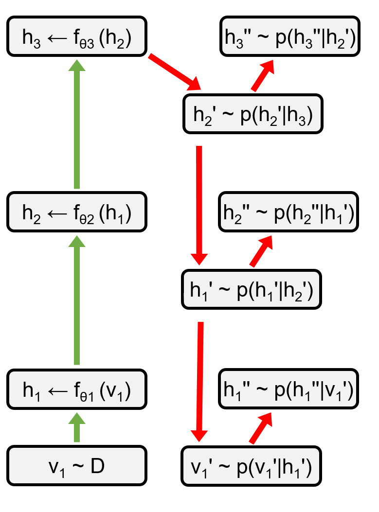
For the sake of our argument, it is useful to make an explicit distinction between bottom-up recognition connections and top-down generative processing (represented by green and red arrows, respectively, in Figure 1). During the recognition (also called “inference”) phase, the sensory pattern is clamped on the visible neurons, and the hidden neurons are activated in a bottom-up fashion in order to infer the most likely configuration (i.e., activation pattern over the hidden neurons) that could have produced the observed data. During the generation phase, the visible neurons are not clamped to the data, and all neurons are activated in a top-down fashion in order to produce a plausible activation pattern, that is, to generate a sample from the internal model.
In the classical approach hinton2006fast, the RBM constituting the bottom layer of the DBN is initially trained using the input data. Once this first layer has been fully trained, the weights of the first RBM are “frozen” and the input data set is projected into the activation space of the hidden neurons, thus creating a new training set that is used as input for the second RBM (black arrows in Figure 1(a)). Once training of the second layer is completed, the data projection is made likewise to create the training set for the third layer; the procedure is repeated for all the layers constituting the DBN, as shown in Figure 1(a). Note that the data patterns projected into the deeper layers are created by computing the conditional probability distribution of the hidden neurons given the activation of the neurons observed in the layer below hinton2012.
2.1.2 Iterative joint learning
In contrast to the greedy approach, the proposed iDBN learning algorithm attempts to update at once all the parameters of the hierarchical generative model, regardless of the depth of the respective layer (see Figure 1(b)).
As noted before, in the greedy algorithm deeper layers are trained sequentially, using as input the projection of the data through the weights resulting from learning in the previous layers. In our novel iterative algorithm, instead, the training patterns for the deeper layers are immediately created following each sensory experience, by propagating the input across the entire processing hierarchy (green arrows in Figure 1(b)). This process mimics the fast feed-forward sweep observed in cortical circuits, where neuronal activity is rapidly routed to a large number of visual areas after stimulus presentation lamme2000distinct; vanrullen2007power. It should be noted that in our algorithm the complete feed-forward sweep occurs even during the initial learning phase, where all the connection weights are randomly initialized, which makes learning of the subsequent layers challenging since the data distribution (i.e., hidden unit activation) is non-stationary. Concurrently with the fast feed-forward sweep, top-down generative connections are locally used to reconstruct the data representations at each level of the hierarchy (red arrows in Figure 1(b)), mimicking the kind of processing supported by recurrent and horizontal connections within cortical areas lamme2000distinct; kreiman2020beyond11
1
It should be noted that, following the initial feed-forward sweep, the generative phases at subsequent levels of the hierarchy still occur sequentially, because the model-driven activation of hidden neurons at layer should not interfere with model-driven activation of the same neurons at layer . Other families of generative models, such as the Deep Boltzmann Machine salakhutdinov2009deep, resolve this potential interference by incorporating top-down influences during learning, but nevertheless require a greedy training strategy..
A schematic pseudo-code that illustrates the implementation details of our iterative algorithm is reported below22
2
The complete source code is freely available to download:
https://github.com/MatteoZambra/Developmental-Approach-DBN.
2.1.3 Full-stack joint learning
An alternative way to jointly learn all weights of a DBN could be to first propagate the input across the entire processing hierarchy (as in the first phase of iDBN) and then produce top-down reconstructions starting from the deepest layer back to the sensory layer (see Figure 1(c)). This processing scheme is simpler to implement, but suffers from the vanishing gradient problem encountered in standard deep learning settings bengio1994. We use this full-stack developmental scheme as a benchmark for our iterative developmental scheme.
2.2 Simulations
2.2.1 MNIST data set
The same DBN structure is used and held fixed during the simulations for both greedy and iterative learning. In order to allow for a fair comparison, we maintained the same architecture and hyper-parameters of the original model hinton2006fast, which was composed of one visible layer with 784 neurons, two hidden layers with 500 neurons each and a final hidden layer with 2000 neurons (see Figure 1(a)). Connection weights are initialized with random values sampled from a Normal distribution , while biases are intialized to zero. We also tested an alternative initialization scheme known as the Glorot initialization glorot2010, in order to evaluate learning convergence under more advanced weight initialization strategies. The weights matrices initialized with the Glorot scheme are multiplied by a factor of to make them compatible with the range observed in the Normal initialization. The learning rate is set to and the weight decay coefficient is set to . The momentum parameter is set to in the initial learning stage and then updated to after 5 epochs of training. The loss is minimized using standard stochastic gradient descent, implemented through CD1 learning. The model is trained for 50 epochs. Further tests, using both Normal and Glorot initialization schemes, also included dropout regularization srivastava2012 with the probability of unit presence set to .
The first quantity inspected to evaluate the quality of the learned models is the accuracy of a linear readout at each hidden layer: since in DBNs the input patterns are non-linearly transformed from one layer to the next one, the internal representations are supposed to become more linearly separable as we move up in the hierarchy zorzi2013modeling. The accuracy of a simple Ridge classifier is used as a measure of separability.
The performance of the trained models is then assessed in three image generation tasks: 1) reproduction of clean images, 2) completion of partially occluded images and 3) denoising of images corrupted by noise. In the second case, an arbitrary number of subsequent rows in the image matrix are set to zero (i.e., turned to black). In the latter case, all values (being 28 the number of side-pixel of the images) are spoiled by adding Gaussian noise, that is , . Images are fed to the visible layer of the DBN, propagated through all its hidden layers and then fed back to the visible layer through feedback connections. In this way the noisy / corrupted samples can be adjusted according to the internal model learned by the DBN. Original samples and the corresponding reconstructions are quantitatively compared using mean squared error (hereafter MSE) between input patterns and reconstruction. For each case, the error is computed as , where the superscript denotes the original sample and means that the image has been reconstructed (reproduced, recreated or denoised) and denotes an norm. Model performance is averaged over 10 model runs with different random initialization in order to assess the robustness of the analyses. We also visualize the receptive fields of neurons at different hidden layers to qualitatively assess the type of features (i.e., internal representations) learned by the DBNs.
2.2.2 Continual learning
To further support the cognitive validity of our approach, we investigate whether the proposed developmental algorithm could effectively deal with a challenging continual learning scenario, where the DBN should learn a generative model of data distributions provided incrementally, without forgetting knowledge obtained during the preceding stages. In such scenario it is well-known that neural networks suffer from catastrophic forgetting, whereby knowledge learned during the subsequent stages completely disrupts previously learned information (for review, see french1999catastrophic). Several solutions have been proposed to mitigate this issue, and here we specifically consider one that can be readily implemented within our framework: interleaved learning complementarySystems2016. We consider a somewhat simplified version of interleaved learning, where unsupervised learning during a second training phase takes advantage of both patterns from the new target distribution and patterns belonging to the previous data set. More advanced implementations could exploit deep generative replay generative2017 to directly sample previously-learned patterns from the hierarchical generative model, allowing to build the mixed dataset in a more data-efficient way.
Following the first stage of unsupervised learning on handwritten digits, the DBN is exposed to a subset of handwritten letters from the EMNIST data set emnist2017. In one setup the DBN is trained sequentially, which means that only letter patterns are used to train the network during the second stage. In the interleaved setup, instead, during the second stage the unsupervised training set includes both digits and letters. In order to balance the number of patterns and output classes, we randomly sample 20,000 digits from the MNIST data set and we evenly sample 20,000 uppercase letters from the first 10 EMNIST classes. Continual learning performance is probed by monitoring both digit recognition accuracy (using the read-out classifier trained during the first learning stage) and letter recognition accuracy (training a new read-out classifier on the EMNIST patterns).
2.2.3 Graph analysis
Recent work has shown that graph theory can be successfully used to study deep learning models from a network science perspective testolin2019; zambra2020. In order to investigate how topological properties of the graph derived from the DBN might emerge during the course of unsupervised learning, we thus performed a graph analysis on the structure of the deep network during learning over the MNIST data set.
From the trained DBN we extract the weights matrices and define a graph having the same architecture and connections weights as the DBN. A methodological difficulty is posed by the continuity of the connection weights: in order to determine the nodes degrees, we thus prune the network by binarizing the connections according to a suitably chosen cut-off threshold. A sensible choice of the cut-off threshold is a value that allows to remove redundant connections and to keep those that contribute most to the signal propagation through the network. Note that the concept of “redundant” and “important” connections is largely arbitrary and not obvious to assess. For the sake of the structural analysis, however, this choice is based on the numerical magnitude of the connections strengths. A range of such thresholds has been set to , and structural analysis has been performed for each of these values. A cut-off threshold of discards the weights in the interval , while those outside the interval are kept for the network analysis.
As customary in network science, the structural properties of the “real” networks (DBNs) are compared with the same properties observed in a random counterpart. A random “replica” of the network is generated according to its architectural characteristics (such an number of nodes) and its local properties (e.g., mean node degree or edge probability). The process is composed of two main steps: 1) generate a random replica of the real network and 2) perform the structural analyses on both the instances. In our case, the real network was compared with an analogous binomial graph generated using the probability of edge existence, computed as the ratio between number of effective edges and the maximum number of potential edges (which depends of the number of node couples). This random replica is generated in such a way to have the same architecture of the DBN, in particular it is a stack of bipartite binomial graphs with the same number of nodes as the DBN layers. Due to this architecture, the node connectivity is constrained by the number of nearby layers. For example, one node of the first layer is not allowed to be connected with one node of the third layer or superior. Such graph structure poses a problem in the characterization of the nodes degree distribution, which is used in network science to evaluate whether a graph is random or derived from a real network. These latter (might them be natural, biological, technological or social networks) typically have a degree distribution well described by a power-law barabasi1999, while random graphs have a degree distribution that depends on the method they are generated with. For example, binomial random graphs have a degree distribution that follows, by design, the Binomial distribution. In our setup, the constrained nodes connectivity would lead the normalization of the degree distribution to have such architectural bias. To mitigate this effect, we chose to weight the degree of each node according to its potential maximum degree, as described in detail in the Appendix C.
2.2.4 Numerosity data set
The “numerosity” data set was first introduced by Stoianov and Zorzi stoianov2012, who demonstrated that the approximate number of objects in a visual scene can be estimated by a hierarchical processing architecture that learns to extract increasingly more abstract representations from the sensory input in a completely unsupervised way (sample images are provided in Figure A.1). Here we focus on the development of “number acuity” in the network, which has been recently investigated using a developmental approach based on deep autoencoders testolin2020numerosity. Number acuity can be measured using a numerosity discrimination task, where the network is asked to classify any image in terms of containing a larger or smaller number of objects with respect to a given reference number. Also in this case, to ensure a fair comparison with the original model stoianov2012, we considered the same model architecture and task. The DBN is composed by a visible layer composed of visible neurons, while the first and the second hidden layers have and neurons, respectively. We adopted a Normal initialization scheme, where weights are initialized with random values sampled from . The learning rate and weight decay are set to and , respectively, and the initial and final momentum are set to and , again with a momentum switch at epoch . The model is trained for 100 epochs.
To assess the number acuity of the network (also known as “internal Weber fraction”), a linear classifier is applied to the deepest layer of the model, with the goal of establishing whether the hidden neurons’ activation correspond to an input image containing a numerosity larger than a reference number (i.e., or ). This task becomes trivial in the limit of the difference between the given numerosity and the reference number being large. For example, it is easier to tell which numerosity is smaller among and , but it is harder for and . For this reason, each reference numerosity has an associated window of numerosities used for the comparison: for and for , so that the ratios yield the range . The percentage of correct classifications is analysed as a function of these numerical ratios: each value has associated the percentage of correct classifications . This ensemble of points is used to fit a psychometric function corresponding to a logistic curve, defined by
| (1) |
being the cumulative distribution function of the Normal distribution and the Weber fraction.
Our interest is to compare the progressive refinement of the Weber fraction during the unsupervised learning phase. The final performance can be directly compared with the Weber fraction achieved by a DBN trained using the greedy scheme stoianov2012, while the developmental trajectories can be compared to the learning curves recently reported for deep autoencoders testolin2020numerosity.
3 Results
3.1 MNIST data set
3.1.1 Readout accuracy and reconstruction error trends
Results discussed in this section only refer to the DBN configuration with Normal initialization and no dropout, since it turned out that differences with Glorot initialization and inclusion of dropout are negligible. The reader may refer to appendix B for the complete results.
Figure 2(a) shows that the readout accuracy increases with depth, suggesting that during the course of unsupervised learning the internal representations became more disentangled (i.e., linearly separable). The reconstruction errors (MSE at each hidden layer) keep decreasing monotonically and eventually converge (Figure 2(b)). Not surprisingly, results related to the first layer are almost perfectly overlapping for the greedy and iterative learning schemes: the activation of the visible layer corresponds to the raw data in both cases, thus the learned weights do not depend on the training modality. For the second and third layers, instead, the greedy scheme achieves higher readout accuracy in fewer epochs: however, this effect is due to the fact that the previous layers have been already completely trained, thus providing a head-start for the upper layers. At the end of training, the final accuracy is indistinguishable. Notably, the alternative developmental variant based on full-stack propagation does not exhibit the same optimal convergence, as highlighted by the poor reconstruction error measured in the first hidden layer (see Figure A.2).
3.1.2 Generative capabilities
As shown in Figure 2(c), at the end of the learning phase the greedy and iterative DBNs achieve equivalent generative capabilities (samples of generated images are provided in Figure A.3). The completion task appears as the more challenging, probably because when entire regions of the images are corrupted it is difficult to generate plausible completions. The full-stack developmental version does not converge to a satisfactory generative model, as highlighted by its poor capability in all generation tasks.
3.1.3 Emergent internal representations
Receptive fields are useful to qualitatively inspect what kind of features are learned by the different layers of the hierarchical model during training. Such inspection is done by visualizing the connection weights of a given neuron in the input space zorzi2013modeling. The first hidden layer is easy to inspect, since we just need to plot the weights matrix of the first layer . When it comes to neurons of the second hidden layer it is necessary to compose the weights matrices, so that it is still possible to represent the visualization in terms of the visible layer dimension. The weights matrices are simply multiplied, thus producing a linear combination: we can simply plot some chosen rows of the product to look at the receptive fields of the second layer neurons, for the third layer, and so forth. As shown in Figure A.4, the greedy and iterative learning schemes developed qualitatively similar receptive fields across the entire processing hierarchy.
3.1.4 Resilience to catastrophic interference
As clearly shown in Figure 3, the sequential learning setup (dashed lines) is dramatically affected by catastrophic interference: while the read-out accuracy on the new letter data set increases, the performance of the classifier trained on the previous digits data set steadily drops as learning proceeds. On the contrary, the interleaved learning setup (solid lines) allows to easily incorporate knowledge from the new letter data set, achieving the same accuracy of the sequential setup, at the same time allowing to maintain previously learned knowledge, as demonstrated by the preservation of the read-out accuracy for the digit data set.

3.1.5 Emergence of structural properties during learning
Typically, inspecting the degrees distribution of a given network gives a first idea of the nature of the system, at least to determine whether the network is random or real. Here, our main focus is on how the structural properties (among the other, also the mean degree) are affected by the learning dynamics. The degree distribution itself is not informative about the structural evolution that the network experiences during training but still could give useful insights about the structural differences of each network. We chose to track other global properties, e.g. mean degree, mean geodesic distance and number of connected components. Figure 4 displays these quantities, while Appendix C provides a broad explanation on the degrees distribution and how to approach its evaluation in this constrained-architecture setup.
Results suggest that the deep network undergoes a substantial transformation during unsupervised learning. A major difference lays in the mean degree evolution during training. Referring to Figure 4(a), non-trivial network properties tend to emerge in later stages of learning, especially for the greedy network. This suggests that the iterative implementation favors the development of complex circuits within the network connections and eventually the emergence of larger components. This applies both to the mean degree and to the number of connected components (recall that an isolated node itself is considered a component). The visualization of the mean geodesic distance shows that the evolution of this property is similar in both the greedy and iterative cases, in particular we can observe a phase transition between an initial state in which all nodes are isolated (indeed an isolated node is considered a component in which the geodesic distance is zero) to the emergence of some components. Once the different component connect to each other and the connections strengthen, the mean geodesic distance decreases.
The second set of results, in Figure 4(b), displays the evolution of the same properties in the binomial replicas. The names “binomial greedy” and “binomial iterative” mean that the binomial counterparts are obtained using the probabilities of edge existence derived from the real greedy and iterative networks, in the epochs considered. The main difference is that both the greedy and iterative instances display the same overall behavior. Unsurprisingly, the visualizations of mean degree and connected components practically overlap. This expected results is given by the fact that there is no such thing as the effect of a learning dynamics that shapes the networks internal structure. In addition, the bottom panels (connected components) show that in random networks the formation of only one giant component is strongly encouraged. Note further that mean degree and mean geodesic distances attain larger values in binomial networks. This is indeed what one could expect: random networks do not have hubs, i.e. nodes with a larger degree with respect to the vast majority of the other nodes, which are instead a characteristic of real scale-free networks. The absence of few super-connected nodes implies a larger mean degree.
The results discussed above refer to the evolution of global network properties. As mentioned before, in network science it is well known that real networks exhibit a power-law degree distribution. As a further comparison between the real networks and their binomial counterparts, we thus choose to also inspect the degree distribution in both the greedy and iterative cases. For this test, we analyze the networks at the end of training and we also include the results obtained with the implementation of dropout, to see if the sparsity induced by dropout changes the network structure. Figure 5 shows the visualization of the degree distributions for real and binomial graphs for the case of Normal initialization, both with and without dropout. The effect of the architectural bias discussed above is particularly clear on the two leftmost upper and lower panels, despite the implementation of the modified degree distribution that accounts for the maximal potential connectivity for each node. This result suggests that the modified degree distribution should be further refined in order to model more accurately the distribution of nodes degrees; still, the degrees distributions show qualitatively different shapes, suggesting that learning dynamics in DBNs characterizes the derived network as a non-random graph. Interestingly, the effect of dropout is to make random replicas more structurally similar to real networks. The top and down right panels of Figure 5 show that a larger connectivity for a small number of nodes is tolerated also in binomial graphs.
3.2 Numerosity data set
As shown in Figure 6(a) the psychometric function observed at the end of the unsupervised learning phase is well aligned with the results obtained by Stoianov and Zorzi using the greedy training scheme stoianov2012. The authors reported a Weber fraction value of , while we obtained a value of .
Concerning the developmental trajectory, as shown in Figure 6(b) the Weber fraction trend displays a significant decrease during the learning period, especially at the early stages of development. This trend is similar to that observed during human development halberda2008developmental; piazza2010developmental. Note that our curve has been obtained by averaging model runs, training different classifiers for each data point to collect more reliable statistics. Thus, the average values account for a population of data points for each sample epoch. It is interesting to note that in the early stages the network might yield a worsening of the performance, and hence highly varying values of . The behaviour stabilizes to an asymptotic value in more advanced learning stages.
Figures 6(c) and 6(d) display the same data points, along with a power-law fit obtained using the method proposed by Testolin, Zou and McClelland testolin2020numerosity. Due to the initial zero value of the epoch time stamp, the basic functional form is actually a modified power-law reichert2013charles:
| (2) |
The parameters , and are fitted to the data points describing the progressive development of the Weber fraction. The resulting parameters are reported in Table 1: the fit closely follows the trajectory of Weber fraction, hence describing satisfactorily well the development of the number sense across the learning period of our networks.
| SZ | ||||
|---|---|---|---|---|
| TZM |
4 Discussion
Our simulations demonstrate that deep belief networks can be trained iteratively, by jointly adjusting all the weights of the model hierarchy following observation of each sensory pattern (or minibatch of patterns). This innovative learning algorithm can be used in place of the traditional greedy, layer-wise learning algorithm in order to accurately track the developmental trajectory of the model. This allows to study how global properties of the network can gradually emerge during the course of learning, at the same time enabling a systematic comparison with biological developmental trajectories observed in empirical studies.
The proposed algorithm was first evaluated on the popular MNIST benchmark, where DBNs trained using the greedy algorithm have traditionally achieved very good performance. We showed that the DBN trained using our iterative algorithm was able to achieve a performance comparable to the greedy counterpart, both in terms of readout accuracy from the internal representations and in terms of reconstruction capabilities. We also probed the final models on a variety of generative tasks, which assessed the DBN ability to reproduce, complete and denoise corrupted input images. Also in this case, we did not observe significant differences between the greedy and iterative versions of the learning algorithm. On the contrary, the attempt to implement joint training of all weights by simply propagating signals across the full stack both in the bottom-up and top-down learning phases led to poor convergence and unsatisfactory results. This reveals that, subsequently to the feed-forward propagation across the entire DBN hierarchy (which resembles the fast feed-forward sweep observed in cortical circuits lamme2000distinct; vanrullen2007power), neurons’ activation at the deepest layer cannot be fed all the way back to the visible layer in a (symmetrical) fast feedback sweep but need to be locally processed at each layer to compute the learning signals (as implemented in the iDBN). Notably, the latter scheme is also consistent with local recurrent processing supported by recurrent and horizontal connections within cortical areas lamme2000distinct; kreiman2020beyond.
To further support the cognitive plausibility of the proposed developmental scheme, we also implemented a straightforward interleaved training approach to tackle continual learning tasks, demonstrating that the iDBN can be also extended to challenging scenarios that require to incrementally incorporate new knowledge in the deep network. This paves the way to the investigation of more plausible continual learning schemes that exploit the top-down generative properties of the DBN to sample the stimuli that are needed for interleaved training calandra2012. Moreover, we carried out an extensive analysis on the progressive development of structural properties in the DBN, by investigating the emergence of a variety of graph-theoretical properties, such as degree, geodesic distance and connected components. Our iterative learning approach allowed to emphasize the gradual refinement of these properties at the global level, thus opening the possibility to more systematically study the topological development of such complex hierarchical systems.
We finally evaluated our iterative approach on a data set that has been recently exploited in a variety of cognitive models to simulate the perception of visual numerosity. Also in this case, the iDBN achieved a final accuracy comparable to the greedy counterpart, at the same time allowing for a precise tracking of the progressive development of the internal representations of the model. Behavioral performance, supported by a linear read-out from the internal representations, can also be continuously tracked to monitor skill acquisition. Indeed, the learning curves resulting from our approach closely resemble the learning curves reported in experimental studies with human children, and also overlap with those reported in a recent developmental model based on deep autoencoders.
5 Conclusion
The scope of the present work was twofold. On the one hand, we presented a novel unsupervised learning algorithm for deep belief networks that allows to accurately track the progressive development of the internal representations of the model. We validated our algorithm on two prototypical benchmark domains, achieving results comparable to the state-of-the-art. On the other hand, we demonstrated that our iterative learning algorithm can be extended to more realistic learning scenarios, at the same time supporting the psychometric analysis of progressive changes in behavioral performance and the study of the gradual development of network properties from the point of view of network theory.
Future studies might take advantage of the proposed iterative algorithm to investigate how the emergence of developmental disorders can be related to impairments in both the initial conditions of the system and the subsequent learning phases. This would be particularly relevant for the study of widespread learning disabilities such as dyscalculia, for which we are still lacking a computational characterization zorzitestolin2022. It would also be useful to explore whether the proposed iDBN approach could be applied in other cognitive domains involving unsupervised deep learning. This would be valuable not only from a machine learning standpoint, but also from a cognitive modeling perspective: Indeed, our iterative algorithm allows to create developmental models that can be quantitatively validated against empirical data collected on humans. Similarly, the proposed graph analysis could be applied in developmental physiology to better understand how structural and functional properties of self-organizing networks might gradually emerge from unsupervised learning dynamics.
Appendix A Supplementary Figures


Appendix B Robustness of the iterative learning scheme results
Results discussed in the main text about the equivalence in terms of performance between greedy and iterative training were focused on the Normal initialization configuration, with no dropout. To assess the robustness of our analyses, here we show that the same results are found when the weights are sampled à la Glorot and when dropout is added as a regularizer.
B.1 Glorot initialization and dropout
Figure B.1 reports the readout and reconstruction profiles obtained with the Glorot initialization. The results show consistency with those presented in the main text. As mentioned before, the weight matrices are down-scaled by a factor in such a way to bring these weights values in a range similar to the weights of Normal initialization.
We also evaluated the effect of dropout on our training scheme. Dropout is an effective regularization method that can be applied to RBMs srivastava2012. The idea is to randomly silence some neurons during training, in such a way to prevent connections to over-learn. This can yield improved generalization capability, though in some cases it might also hinder learning performance. Bottom panels in Figure B.1 shows that also in this setup the overall performance of the model is not affected.
(Glorot, no dropout)
(Normal, dropout)
(Glorot, dropout)
Appendix C Graph analysis in depth
In Section 2.2.3 we discussed the critical choice of the cut-off threshold and displayed aggregated data of the emerging global structural properties. Here the degrees distributions are discussed in finer-grained detail, since the graph structure extrapolated from a DBN poses some case-specific problems. Indeed, it is not straightforward to choose a model distribution to fit the emergent weights configuration, since during learning some connection strengths are significantly increased, leading to long-tail frequency distributions. Rather than searching or producing an ad-hoc probability distribution for the learned weights and then pruning the network according to some distribution-specific values (e.g. quantiles), an heuristic choice is rather to prune the network based on a user-defined cut-off threshold. In Section 2.2.3, a set of such meta-parameters is used jointly with the reference epochs to draw mean degrees, distances and connected components maps. Here the focus is on the degree distribution for a given cut-off threshold, which has different characteristics in random graphs and real networks barabasi2016.
C.1 Degrees distribution
Real networks typically exhibit a degree distribution than follows a power-law, expressed by:
| (3) |
where represents the degree, is the decaying exponent and is a constant. Results in Figure 5 were obtained by eliminating all the weights in the interval , thus excluding the majority of connections. The power-law fit performs poorly for these DBN-like networks and the shape of the distribution deviates from the linear trend typical of scale-free networks, creating issues with the empirical way of computing the degrees distribution. Typically, one would count all the nodes having degree , call this quantity . The fraction of such nodes is:
| (4) |
where is the number of nodes in the network and is the fraction of nodes having degree . This expression identifies a legitimate probability mass function, since . The network architecture poses a subtle problem: while in real networks any node could be connected to virtually any other, here each node can be connected to all and solely those belonging to neighboring layers. Thus, each node should be associated with a potential maximum degree. This quantity is used to correct the degrees distribution, by penalizing a node depending on its maximum allowed connectivity, thus smoothing the resulting distribution. The nodes fraction is set to:
| (5) |
where is the indicator function. This distribution is normalized computing the normalizing function numerically as . Assume that node has degree . Its relevance in the number of nodes is weighted with its potential maximum degree, computed as the sum of the row of the adjacency matrix . The aim of this model is to normalize the nodes degrees according to the potential maximum degree of each node.
C.2 Binomial replicas
To make the analysis more robust, we experiment a comparison with a synthetic null model having the exact same architecture as the DBN, created as a Binomial Random Graph (also known as Erdős-Renyj model, ER hereafter, newman2003). The comparison between the degrees distributions of real network and binomial replicas is displayed in Figure 5 in the main text. To generate the random network counterparts , the same architecture of the real network is used. The probability of edge existence is then computed as the ratio between the number of the actual edges (once the network has been pruned) and the total number of connections (given by the architecture), latora2017. The same probability is used to generate random links between all the four layers of nodes of the random network produced. The resulting replicas are random, but not strictly binomial: the degree distribution inevitably deviates from the Poissonian trend, and this is not (only) due to the fact that the number of nodes is relatively small (3784 nodes), but rather to the network bipartite structure.
C.3 Correction of degrees distribution
Due to architectural constraints, it is not possible to observe the idealized power-law and binomial degrees distributions for our networks. Binomial networks have a binomial degrees distribution and the probability mass function is expressed by:
| (6) |
which means that a given node has links with probability , out of a total of links it could have if the network was fully connected, i.e. . The number of connections of a given node ranges between virtually zero and its potential maximum degree, which is the total number of neurons of the neighboring layers.
We propose a correction to normalize the node degrees in such a way to correct the architectural bias. The strategy chosen for generating the results in the main text is that of Equation 5, however the choice of this model is not unique. For example, we could choose a model that sets the fraction of nodes having degree to the corrective factor previously multiplied by :
| (7) |
again being the full-graph adjacency matrix. This fraction can be computed easily, then the actual distributions are computed normalizing the raw fractions and as follows:
| (8) |
The two model distributions have been chosen performing some observation on completely random graphs, completely independent of the probabilities of edge existence of the real network. The first synthetic graph shares the same architecture of the DBN, with tunable probability of existence , chosen small. A second test case involves a bipartite random graph with the same number of nodes on both sides. The third test case involves a bipartite graph having and nodes on the two sides. The goal is to compare qualitatively both the distributions and on these three test cases to check whether one or the other model distributions perform better. Figure C.1 displays the results of these simulations. The experiments reveal that adheres better to the Poissonian trend, thus motivating the choice of the model distribution for the analyses presented in the main text.
Acknowledgements.
We are grateful to Michele De Filippo De Grazia for support with the simulations related to continual learning, and to Ivilin Stoianov for useful discussions about the iterative version of the developmental algorithm presented in this paper. Author Contributions A.T. and M.Zo. contributed to the study conception and design. Computational simulations, data collection and analysis were performed by M.Za. The first draft of the manuscript was written by M.Za. and A.T. All authors commented on previous versions of the manuscript, and all authors read and approved the final manuscript. Compliance with Ethical Standards Ethical approval: This article does not contain any studies with human participants or animals performed by any of the authors. Funding: This work was supported by a Cariparo Excellence Grant 2017 (project “Numsense”) to M.Zo. Data Availability Statement The complete source code of the iterative learning algorithm and additional data related to the analyses discussed in the current study are freely available though the following repository: https://github.com/MatteoZambra/Developmental-Approach-DBN.References
- (1) Y. LeCun, Y. Bengio, and G. E. Hinton, “Deep learning,” Nature, vol. 521, 2015.
- (2) G. E. Hinton, S. Osindero, and Y.-W. Teh, “A fast learning algorithm for deep belief nets,” Neural computation, vol. 18, no. 7, pp. 1527–1554, 2006.
- (3) G. E. Hinton and R. R. Salakhutdinov, “Reducing the dimensionality of data with neural networks,” science, vol. 313, no. 5786, pp. 504–507, 2006.
- (4) H. Lee, R. Grosse, R. Ranganath, and A. Y. Ng, “Convolutional deep belief networks for scalable unsupervised learning of hierarchical representations,” in Proceedings of the 26th annual international conference on machine learning, pp. 609–616, 2009.
- (5) A.R. Mohamed, G. E. Dahl, and G. Hinton, “Acoustic modeling using deep belief networks,” IEEE transactions on audio, speech, and language processing, vol. 20, no. 1, pp. 14–22, 2011.
- (6) W. Huang, G. Song, H. Hong, and K. Xie, “Deep architecture for traffic flow prediction: deep belief networks with multitask learning,” IEEE Transactions on Intelligent Transportation Systems, vol. 15, no. 5, pp. 2191–2201, 2014.
- (7) A. M. Abdel-Zaher and A. M. Eldeib, “Breast cancer classification using deep belief networks,” Expert Systems with Applications, vol. 46, pp. 139–144, 2016.
- (8) Y. Du and I. Mordatch, “Implicit generation and generalization in energy-based models,” arXiv preprint arXiv:1903.08689, 2019.
- (9) J. Tubiana and R. Monasson, “Emergence of compositional representations in restricted boltzmann machines,” Physical review letters, vol. 118, no. 13, p. 138301, 2017.
- (10) R. G. Melko, G. Carleo, J. Carrasquilla, and J. I. Cirac, “Restricted boltzmann machines in quantum physics,” Nature Physics, vol. 15, no. 9, pp. 887–892, 2019.
- (11) M. Zorzi, A. Testolin, and I. P. Stoianov, “Modeling language and cognition with deep unsupervised learning: a tutorial overview,” Frontiers in psychology, vol. 4, p. 515, 2013.
- (12) K. Friston, “The free-energy principle: a unified brain theory?,” Nature Reviews Neuroscience, vol. 11, p. 127-138, 2010.
- (13) A. Testolin and M. Zorzi, “Probabilistic models and generative neural networks: Towards an unified framework for modeling normal and impaired neurocognitive functions,” Frontiers in Computational Neuroscience, vol. 10, p. 73, 2016.
- (14) I. Stoianov and M. Zorzi, “Emergence of a “visual number sense” in hierarchical generative models,” Nature neuroscience, vol. 15, pp. 194–6, 02 2012.
- (15) M. Zorzi and A. Testolin, “An emergentist perspective on the origin of number sense,” Philosophical Transactions of the Royal Society B: Biological Sciences, vol. 373, no. 1740, p. 20170043, 2018.
- (16) A. Testolin, S. Dolfi, M. Rochus, and M. Zorzi, “Visual sense of number vs. sense of magnitude in humans and machines,” Scientific reports, vol. 10, no. 1, pp. 1–13, 2020.
- (17) A. Testolin, I. Stoianov, and M. Zorzi, “Letter perception emerges from unsupervised deep learning and recycling of natural image features,” Nature human behaviour, vol. 1, no. 9, pp. 657–664, 2017.
- (18) Z. Sadeghi and A. Testolin, “Learning representation hierarchies by sharing visual features: a computational investigation of persian character recognition with unsupervised deep learning,” Cognitive processing, vol. 18, no. 3, pp. 273–284, 2017.
- (19) M. G. Di Bono and M. Zorzi, “Deep generative learning of location-invariant visual word recognition,” Frontiers in psychology, vol. 4, p. 635, 2013.
- (20) B. J. Grzyb, Y. Nagai, M. Asada, A. Cattani, C. Floccia, and A. Cangelosi, “Children’s scale errors are a natural consequence of learning to associate objects with actions: A computational model,” Developmental science, vol. 22, no. 4, p. e12777, 2019.
- (21) D. P. Reichert, P. Series, and A. J. Storkey, “Charles bonnet syndrome: evidence for a generative model in the cortex?,” PLoS Comput Biol, vol. 9, no. 7, p. e1003134, 2013.
- (22) H. Lee, C. Ekanadham, and A. Y. Ng, “Sparse deep belief net model for visual area v2,” in Advances in neural information processing systems, pp. 873–880, 2008.
- (23) L. Buesing, J. Bill, B. Nessler, and W. Maass, “Neural dynamics as sampling: a model for stochastic computation in recurrent networks of spiking neurons,” PLoS Comput Biol, vol. 7, no. 11, p. e1002211, 2011.
- (24) P. O’Connor, D. Neil, S.-C. Liu, T. Delbruck, and M. Pfeiffer, “Real-time classification and sensor fusion with a spiking deep belief network,” Frontiers in neuroscience, vol. 7, p. 178, 2013.
- (25) G. Pezzulo, M. Zorzi, and M. Corbetta, “The secret life of predictive brains: what’s spontaneous activity for?,” Trends in Cognitive Sciences, vol. 25, p. 730-743, 2021.
- (26) P.R. Huttenlocher and A.S. Dabholkar, “Regional differences in synaptogenesis in human cerebral cortex,” The Journal of Comparative Neurology, vol. 387, p. 167–178, 1997.
- (27) E. Castaldi, C. Lunghi, and M.C. Morrone, “Neuroplasticity in adult human visual cortex,” Neuroscience and Biobehavioral Reviews, vol. 112, p. 542–552, 2020.
- (28) P. Fransson, B. Skiöld, S. Horsch, A. Nordell, M. Blennow, H. Lagercrantz, and U. Åden, “Resting-state networks in the infant brain,” Proceedings of the National Academy of Sciences, vol. 104, p. 15531-15536, 2007.
- (29) J.L. Elman, E. Bates, and M.H. Johnson, Rethinking innateness: A connectionist perspective on development, MIT Press, 1996.
- (30) M. Zorzi and A. Testolin, “Computational models of typical and atypical development of reading and numeracy,” in The Cambridge Handbook of Dyslexia and Dyscalculia, Cambridge University Press, 2022.
- (31) A. Testolin, W. Y. Zou, and J. L. McClelland, “Numerosity discrimination in deep neural networks: Initial competence, developmental refinement and experience statistics,” Developmental Science, p. e12940, 2020.
- (32) D. E. Rumelhart, G. E. Hinton, and R. J. Williams, “Learning representations by back-propagating errors,” Nature, vol. 323, no. 6088, pp. 533–536, 1986.
- (33) G. Hinton, “Training products of experts by minimizing contrastive divergence,” Neural computation, vol. 14, pp. 1771–800, 2002.
- (34) Y. LeCun, L. Bottou, Y. Bengio, and P. Haffner, “Gradient-based learning applied to document recognition,” Proceedings of the IEEE, vol. 86, no. 11, pp. 2278–2324, 1998.
- (35) G.I. Parisi, R. Kemker, J.L Part, C. Kanan, and S. Wermter, “Continual lifelong learning with neural networks: A review,” Neural Networks, vol. 113, pp. 54-71, 2019.
- (36) M. McCloskey and N.J. Cohen, “Catastrophic interference in connectionist networks: The sequential learning problem,” Psychology of learning and motivation, vol. 24, pp. 109-165, 1989.
- (37) R. M. French, “Catastrophic forgetting in connectionist networks,” Trends in Cognitive Sciences, vol. 3, pp. 128-135, 1999.
- (38) D. H. Ackley, G. E. Hinton, and T. J. Sejnowski, “A learning algorithm for boltzmann machines,” Cognitive science, vol. 9, no. 1, pp. 147–169, 1985.
- (39) N. Zhang, S. Ding, J. Zhang, and Y. Xue, “An overview on restricted boltzmann machines,” Neurocomputing, vol. 275, pp. 1186–1199, 2018.
- (40) G. Hinton, “Learning multiple layers of representation,” Trends in cognitive sciences, vol. 11, pp. 428–34, 2007.
- (41) G. E. Hinton, A Practical Guide to Training Restricted Boltzmann Machines, pp. 599–619. Berlin, Heidelberg: Springer Berlin Heidelberg, 2012.
- (42) V. A. Lamme and P. R. Roelfsema, “The distinct modes of vision offered by feedforward and recurrent processing,” Trends in neurosciences, vol. 23, no. 11, pp. 571–579, 2000.
- (43) R. VanRullen, “The power of the feed-forward sweep,” Advances in Cognitive Psychology, vol. 3, no. 1-2, p. 167, 2007.
- (44) G. Kreiman and T. Serre, “Beyond the feedforward sweep: feedback computations in the visual cortex,” Annals of the New York Academy of Sciences, vol. 1464, no. 1, p. 222, 2020.
- (45) R. Salakhutdinov and G. Hinton, “Deep boltzmann machines,” in Artificial intelligence and statistics, pp. 448–455, PMLR, 2009.
- (46) Y. Bengio, P. Simard, and P. Frasconi, “Learning long-term dependencies with gradient descent is difficult,”. IEEE transactions on neural networks, vol. 5, no. 2, pp. 157-166, 1994.
- (47) X. Glorot and Y. Bengio, “Understanding the difficulty of training deep feedforward neural networks,” in Proceedings of the thirteenth international conference on artificial intelligence and statistics, pp. 249–256, 2010.
- (48) N. Srivastava, G. Hinton, A. Krizhevsky, I. Sutskever, and R. Salakhutdinov, “Dropout: A simple way to prevent neural networks from overfitting,” J. Mach. Learn. Res., vol. 15, p. 1929–1958, Jan. 2014.
- (49) G. Cohen, S. Afshar, J. Tapson, and A. Van Schaik, “EMNIST: Extending MNIST to handwritten letters,” in International joint conference on neural networks, pp. 2921–2926, 2017.
- (50) D. Kumaran, D. Hassabis, and J. L., McClelland, “What learning systems do intelligent agents need? Complementary learning systems theory updated,” Trends in Cognitive Sciences, vol. 20, pp. 512-534, 2016.
- (51) H. Shin, J. Lee, J. Kim, and J. Kim, “Continual learning with deep generative replay,” in Advances in neural information processing systems, vol. 30, 2017.
- (52) A. Testolin, M. Piccolini, and S. Suweis, “Deep learning systems as complex networks,” Journal of Complex Networks, vol. 8, 06 2019.
- (53) M. Zambra, A. Maritan, and A. Testolin, “Emergence of network motifs is deep neural networks,” Entropy, vol. 22, 2020.
- (54) A.L., Barabási and R., Albert, “Emergence of scaling in random networks,” Science, vol. 286, pp. 509-512, 1999.
- (55) J. Halberda and L. Feigenson, “Developmental change in the acuity of the number sense: The approximate number system in 3-, 4-, 5-, and 6-year-olds and adults.,” Developmental psychology, vol. 44, no. 5, p. 1457, 2008.
- (56) M. Piazza, A. Facoetti, A. N. Trussardi, I. Berteletti, S. Conte, D. Lucangeli, S. Dehaene, and M. Zorzi, “Developmental trajectory of number acuity reveals a severe impairment in developmental dyscalculia,” Cognition, vol. 116, no. 1, pp. 33–41, 2010.
- (57) R. Calandra,T. Raiko, M. Deisenroth, and F.M. Pouzols, “Learning deep belief networks from non-stationary streams,” in International Conference on Artificial Neural Networks, p. 379-386, 2012.
- (58) A.L. Barabási and M. Pósfai, Network Science. Cambridge University Press, 2016.
- (59) K.L. Du and M. N. Swamy, Neural networks and statistical learning. Springer Science & Business Media, 2013.
- (60) M. E. Newman, “The structure and function of complex networks,” SIAM review, vol. 45, no. 2, pp. 167–256, 2003.
- (61) V. Latora, V. Nicosia, and G. Russo, Complex Networks: Principles, Methods and Applications. Complex Networks: Principles, Methods and Applications, Cambridge University Press, 2017.