Operator growth and Krylov construction in dissipative open quantum systems

Integrability and chaos has remained a long-standing problem in quantum many-body systems. In a closed system, the integrability is marked by a substantial number of conserved quantities PhysRevLett.111.127201; ROS2015420; PhysRevB.91.085425. This shows up in the level statistics of the unfolded spectrum, which follow the Poisson distribution, known as the Berry-Tabor conjecture Berry_Tabor. In contrast, Wigner-Dyson statistics is noticeable for the chaotic systems, often referred to as Bohigas-Giannoni-Schmit (BGS) conjecture Wigner; BGS. However, dissipation and decoherence are ubiquitous in nature, making any evolution non-unitary. The effect of decoherence has been a growing interest in the research of many-body systems, and field theory PhysRevLett.118.140403; Beau:2017xaj; DelCampo:2019afl; Xu:2020wky. Decoherence may not always be associated with the environment. It can happen solely due to the random fluctuations, noise, and random phase changes in the system braun2003dissipative; Xu:2018bhd. Hence, it is of practical interest to extend the notion of integrability and chaos in open systems where the system interacts with the environment. Indeed, Grobe, Haake, and Sommers (GHS) generalized the above ideas to such systems PhysRevLett.61.1899, governed by Markovian dynamics. Instead of the Hermitian Hamiltonian, one considers the level statistics of the corresponding Lindbladian supplemented by the appropriate jump operators, which capture the dissipation. The eigenvalues of the Lindbladian can be real or complex (in pairs), and one can devise an appropriate version of the level statistics. While integrable systems exhibit Poisson statistics, chaotic systems follow the distribution of Ginibre ensemble Ginibre; PhysRevLett.61.1899; PhysRevLett.123.254101; PhysRevResearch.2.023286. Thus, level statistics provides a powerful way to detect non-integrability in open systems.

Operator growth, on the other hand, provides an indirect yet illuminating way to capture such behavior. The idea stems from the fact that under Heisenberg evolution, a simple operator becomes complicated as time progresses. A piece of local information supported on a single or few sites spread to the whole system, leading to the thermalization of chaotic systems PhysRevA.43.2046; PhysRevE.50.888; PhysRevLett.98.050405; Rigol_2008. Depending on whether the Hamiltonian is integrable or chaotic, operators grow differently. Although such growth has been well understood in terms of the out-of-time-ordered functions (OTOC), it has recently been revived by the universal operator growth hypothesis (UOGH) Parker:2018yvk, which extends the operator growth beyond the semi-classical limit. It states that the chaotic systems show the fastest growth of Lanczos coefficients (defined later), although all the systems with the fastest growth may not be chaotic Dymarsky:2021bjq; Bhattacharjee:2022vlt. Recently, the UOGH has gained much interest from the many-body perspective, conformal field theory and holography Avdoshkin:2019trj; Dymarsky:2019elm; Barbon:2019wsy; Rabinovici:2020ryf; Jian:2020qpp; PhysRevE.104.034112; Cao:2020zls; Magan:2020iac; Rabinovici:2021qqt; Yates:2021asz; PhysRevLett.124.206803; PhysRevB.102.195419; Kim:2021okd; Caputa:2021ori; Trigueros:2021rwj; Bhattacharjee:2022vlt; Caputa:2021sib; Patramanis:2021lkx; Hornedal:2022pkc; Heveling:2022hth; Kar:2021nbm; Muck:2022xfc; Banerjee:2022ime; Heveling:2022orr.

In this work, we take a first step to extend the operator growth and the underlying formalism into dissipative open quantum systems. Our setup is the well-known transverse field Ising model (TFIM) interacting with the environment. In order to see the growth, one needs to expand the operator in terms of a Krylov basis. The standard approach is to apply the well-known Lanczos algorithm, which is efficient for the unitary evolution. This is in contrast to the non-unitary evolution of the open systems where the Lindbladian is non-Hermitian. Still, the direct application leads to some intriguing results capturing the breakdown of Hermitian methods in the case of non-Hermitian cases. For the integrable case, as soon as the system starts interacting with the environment, i.e., non-Hermiticity sets in non-trivially, the sublinear growth of the Lanczos coefficients tends to become linear. Furthermore, the growth becomes indiscernible between the integrable and chaotic limit for large Lanczos coefficients, which appears to grow forever. This behavior is clearly unphysical due to the finite-dimensional restriction of the Krylov subspace. This effect of decoherence must be distinguished from chaos Yoshida:2018vly. Hence, we need a more refined algorithm that correctly incorporates such a non-Hermitian effect. The Arnoldi iteration, a well-known iterative algorithm to find the eigenvalues and eigenvectors of non-Hermitian matrices, achieves this. Of course, when the evolution becomes unitary, the Arnoldi iteration reduces to the usual Lanczos algorithm. In the following sections, we ask the question of whether the successful implementation of the Arnoldi iteration truly enables tracking the integrability or chaotic nature of the system. Also, to be fully sensitive to the conditions and parameters involved, we will also ask whether the Arnoldi iteration can distinguish between different values of the non-Hermitian couplings involved in the study. To our satisfaction, we find the answers to both the questions are positive.

The paper is structured as follows. In section 2, we briefly discuss the construction of the Krylov basis. Section 3 introduces the open system, especially the model with computation of Lanczos coefficients, including the dissipative environment. We discuss the details of the Arnoldi iteration in section 4. We conclude the paper with a brief summary and outlook in section 5.

In this section, we briefly review the basic formulation of Lanczos algorithm for the construction of orthonormal Krylov basis viswanath1994recursion; Parker:2018yvk. Consider an initial operator $\mathcal{O}_{0}$ at $t=0$, sometimes known as the seed operator. Under the unitary time evolution governed by a time-independent Hamiltonian $H$, the time-evolved operator $\mathcal{O}(t)$ is written by the Heisenberg evolution as

$$\mathcal{O}(t)=e^{iHt}\,\mathcal{O}_{0}\,e^{-iHt}=e^{i\mathcal{L}t}\mathcal{O}_{0}\,,$$

(1)

where $\mathcal{L}\,[\bullet]=[H,\bullet]$ is the Liouvillian superoperator. The explicit time evolution can be obtained by using the Baker-Campbell-Hausdorff (BCH) formula, which involves nested commutators of the form $[H,[H,\mathcal{O}_{0}],\cdots]$ obtained by the repeated application Liouvillian $\mathcal{L}^{n}\mathcal{O}_{0}$. For a local seed operator $\mathcal{O}_{0}$, these nested commutators indicate the increasing degree of non-locality, and they eventually become extremely difficult to compute. However, one can circumvent this difficulty by constructing an orthonormal set of basis $|\mathcal{O}_{n})$, with $n=0,1,2,\cdots,\mathcal{K}-1$, known as Krylov basis. The dimensionality of the Krylov space $\mathcal{K}$ is constrained to $1\leq\mathcal{K}\leq D^{2}-D+1$ Rabinovici:2020ryf, where $D$ is the dimension of the Hilbert space. This makes the problem much simpler to tackle. On such a basis, the Liouvillian takes the tridiagonal form

$\displaystyle\mathcal{L}|\mathcal{O}_{n})=b_{n}|\mathcal{O}_{n-1})+b_{n+1}|\mathcal{O}_{n+1})\,,$

(2)

where the coefficients $b_{n}$’s are known as Lanczos coefficients with $b_{0}=0$. for a finite-dimensional system with Krylov dimension $\mathcal{K}$, $b_{n}$ halts at $n=\mathcal{K}-1$ with the Krylov basis $|\mathcal{O}_{\mathcal{K}})$ such that $b_{\mathcal{K}}=0$. The evolved operator $\mathcal{O}(t)$ can be expanded as

$$|\mathcal{O}(t))=\sum_{n=0}^{\mathcal{K}-1}i^{n}\phi_{n}(t)|\mathcal{O}_{n})\,,$$

(3)

where the “wavefunctions” $\phi_{n}(t)=i^{-n}(\mathcal{O}_{n}|\mathcal{O}(t))$ mimic the probability density and satisfies the unitarity constraint Parker:2018yvk

$$\sum_{n}|\phi_{n}(t)|^{2}=1\,.$$

(4)

The first wavefunction is known as the auto-correlation function and is given by

$$\phi_{0}=(\mathcal{O}_{0}|\mathcal{O}(t))\,.$$

(5)

It is worth mentioning here that the auto-correlation function can also produce the exact same set of $b_{n}$’s by the method of moments with the corresponding recursion relation Parker:2018yvk. At this stage, one should properly define the inner product $(A|B)$ of two operators $A$ and $B$. One usually considers the infinite-temperature Wightmann inner product given by $(A|B)=\frac{1}{D}\mathrm{Tr}(A^{\dagger}B)$. It is to be noted that the notion of the inner product is not unique^** * An alternate choice of the inner product could be with respect to the non-equilibrium steady state density matrix $\rho_{\mathrm{NESS}}$, so that $\mathcal{L}_{S}\{\rho_{\mathrm{NESS}}\}=0$. This is under the assumption that the Lindbladian has at least one stationary state. Hence, the corresponding definition of inner product will be $(A|B)=\frac{1}{D}\mathrm{Tr}(\rho_{\mathrm{NESS}}A^{\dagger}B)$. On the other hand, the inner product with equilibrium density matrix $\rho_{\infty}=\lim_{t\rightarrow\infty}\rho(t)$ is generically given by $(A|B)\propto\mathrm{Tr}(\rho_{\infty}A^{\dagger}B)$, with $\rho_{\infty}\propto I$, when the jump operators are Hermitian PhysRevB.98.020202. Nevertheless, in this paper, we stick to the choice of the equilibrium infinite temperature inner product. We thank Xiangyu Cao for pointing this out., and one can, in principle, define another set of the inner product. However, this definition is a standard choice in the literature Parker:2018yvk.

The wavefunctions are recursively related by the Lanczos coefficients by a recursive differential equation of the form

$$\dot{\phi}_{n}(t)=b_{n}\phi_{n-1}(t)-b_{n+1}\phi_{n+1}(t).$$

(6)

with $\phi_{-1}(t)=0$ and $\phi_{n}(0)=\delta_{n0}$. This recursion can be visualized as a particle hopping in a lattice where the hopping amplitudes are encoded in the Lanczos coefficients. The average expectation of the particle hopping in the lattice site is defined as the Krylov complexity $K(t)=\sum_{n}n|\phi_{n}(t)|^{2}$, and they contain exactly the same information as the Lanczos coefficients Parker:2018yvk; Barbon:2019wsy. For our purpose, we see that Lanczos coefficients suffice to reach the main conclusion, without the need of computing the Krylov complexity.

In open systems, i.e., systems that interact with the environment, the evolution of operators is subtle. The total Hamiltonian can be separated into three parts

$$H_{\mathrm{SE}}=H_{\mathrm{S}}\otimes I_{\mathrm{E}}+I_{\mathrm{S}}\otimes H_{\mathrm{E}}+H_{I}\,,$$

(7)

where the full dynamics is governed by the system Hamiltonian $H_{\mathrm{S}}$ together with the environment Hamiltonian $H_{\mathrm{E}}$. Here $H_{I}$ denotes the interaction between the system and the environment Breuer2007, and $I_{\mathrm{S}}$ and $I_{\mathrm{E}}$ denotes the identity operators acting on the system and the environment respectively. A simple way to write the interacting Hamiltonian is the following

$$H_{I}=\sum_{i}\alpha_{i}\,S_{i}\otimes E_{i}\,,$$

(8)

where $S_{i}$ and $E_{i}$ are operators in the system, and environment Hilbert space, respectively. $\alpha_{i}$ denotes the coupling associated with this interaction. The open systems are important physically as well as experimentally since the preparation of an ideal isolated system is almost impossible. Hence, most of the experimental setups are essentially open systems with always some interaction with the environment. The dynamics of the entire system is given by the von Neumann equation $\dot{\rho}_{\mathrm{SE}}(t)=-i[H_{\mathrm{SE}},\rho_{\mathrm{SE}}(t)]$, where $\rho_{\mathrm{SE}}$ is the density matrix of the total system. This can also be understood as the equivalent to the Schrödinger equation for the pure state of the full system. The well-known Heisenberg equation of motion of an operator $O_{\mathrm{SE}}(0)$ reads

$$\dot{O}_{\mathrm{SE}}(t)=i[H_{\mathrm{SE}},O_{\mathrm{SE}}(t)]=i\mathcal{L}_{c}O_{\mathrm{SE}}(t)\,,$$

(9)

where $\mathcal{L}_{c}\,\bullet=[H_{\mathrm{SE}},\,\bullet]$ is known as the Liouvillian for the closed system. We are especially interested in studying the dynamics of the system which lives in the Hilbert space $\mathcal{H}_{\mathrm{S}}$. For that, we will consider the reduced density matrix $\rho_{\mathrm{S}}(t)=\mathrm{Tr}_{\mathrm{E}}[\rho_{\mathrm{SE}}(t)]$ by tracing out the degrees of freedom from the environment. The system density matrix evolves as $\rho_{\mathrm{S}}(t)=\sum_{j}E_{j}\rho_{\mathrm{S}}(0)E_{j}^{\dagger}$, where $\rho_{\mathrm{S}}(0)$ is the system density matrix at $t=0$, and $E_{j}$’s are known as the Kraus operators satisfying the normalization $\sum_{j}E_{j}^{\dagger}E_{j}=1$. They incorporate all the information of the environment and have imprints left of their interaction with its environment. Since we are interested in the system dynamics, we want to study operator dynamics in the system part eventually. In other words, our knowledge of the environment is limited to its interaction with the environment through system parameters only. This is expected since, it is impossible to know the detailed dynamics of the full universe.

We are typically interested in the Markovian dynamics which essentially leads to a small time expansion of the form

$$\rho_{\mathrm{S}}(t+dt)=\rho_{\mathrm{S}}(t)+\mathcal{O}(dt)\,.$$

(10)

It means that the system density matrix $\rho_{\mathrm{S}}(t+dt)$ at a time $t+dt$ remembers its past history only infinitesimally up to $\rho_{\mathrm{S}}(t)$. Going forward, we drop the index “S” from the density matrix and it will always imply the system density matrix unless specified otherwise. The Born-Markovian dynamics of the system density matrix is given by the Lindblad master equation Lindblad1976; Gorini

$\displaystyle\dot{\rho}=-i[H,\rho]+\sum_{k}\big[L_{k}\rho L_{k}^{\dagger}-\frac{1}{2}\{L_{k}^{\dagger}L_{k},\rho\}\big]\,,$

(11)

or compactly as $\dot{\rho}(t)=-i\mathcal{L}_{o}\rho(t)$, where $\mathcal{L}_{o}$ is known as the Lindbladian superoperator, $H$ is the Hamiltonian of the system, and $\{\,,\,\}$ is the usual anti-commutator. This can be thought as the generator of a dynamical map $V(t)=e^{i\mathcal{L}_{o}t}$ on the space of the reduced density matrix of the system $V(t):\mathcal{S}(H_{\mathrm{S}})\rightarrow\mathcal{S}(H_{\mathrm{S}})$ and satisfying the semi-group property Breuer2007. The operators $\{L_{j}\}$ are known as the Lindblad or the jump operators which are constructed from the Kraus operators $E_{j}$ in the interaction part of the Hamiltonian $H_{I}$ along with a coupling parameter $\alpha$.

The Schrödinger evolution for the density matrix under the full Hamiltonian $H_{\mathrm{SE}}$ is very similar to the Heisenberg evolution of an operator. Hence, a system operator $O\equiv O(0)$ evolves as $\dot{O}(t)=i\mathcal{L}_{o}O(t)$, where the Lindbladian is Breuer2007; lidar2019lecture

$\displaystyle\mathcal{L}_{o}[\bullet]=[H,\bullet]-i\sum_{k}\big[L_{k}^{\dagger}\bullet L_{k}-\frac{1}{2}\{L_{k}^{\dagger}L_{k},\bullet\}\big]\,,$

(12)

where the subscript “o” indicates that the system is open. Here, as before, $H$ is the system Hamiltonian, thus including the Hermitian part only, and the $\bullet$ can be replaced by any generic operator $O(t)$. Note a significant difference in the Lindbladian from the Liouvillian. The Lindbladian has a non-Hermitian part apart from the usual Hermitian commutator. This results in a non-unitary dynamics of the system state density matrix $\rho$ as well as the system operator $O(t)$. This is a consequence of dissipation coming in due to interaction with the environment. In other words, the smaller the coupling parameters in the non-Hermitian part are, the closer the system is to an isolated system. The dynamics is summarized pictorially in Fig. 1.

The obvious reason for this breakdown and inability to produce physically meaningful results for the Lanczos algorithm seems to be the presence of the non-Hermitian Lindbladian. It is not completely surprising as the original efficiency of the Lanczos algorithm stems from its ability to approximate the eigenvalues of a Hermitian matrix. This calls for an efficient method that extends beyond the Hermitian matrices. A known method in literature is the Arnoldi iteration Arnoldi1951ThePO; Arnoldi2; Minganti:2021gxs for approximating the eigenvalues of a non-Hermitian matrix. In fact, the Lanczos algorithm can be derived as a special case of the Arnoldi iteration when the matrix is symmetric and Hermitian. Instead of subtracting one previous vector as done in the Lanczos algorithm, in Arnoldi iteration, one performs the reduction of all previous vectors. More generally, a two-dimensional array is produced for the matrix form of the Lindbladian in the non-Hermitian case. Recall that the closed system Liouvillian ($\mathcal{L}_{c}\,\bullet=[H,\bullet]$) in Heisenberg picture has a tridiagonal form after implementation of the Lanczos algorithm with only $b_{n}$’s. The form is the following

$$\mathcal{L}_{mn}^{(c)}=(O_{m}|\mathcal{L}_{c}|O_{n})~~~\Rightarrow~~~\mathcal{L}^{(c)}=\begin{pmatrix}0&b_{1}&0&\cdots&0\\ b_{1}&0&b_{2}&\cdots&0\\ 0&b_{2}&0&b_{3}&\cdots\\ \cdots&\cdots&b_{3}&\cdots&\cdots\\ 0&\cdots&\cdots&\cdots&b_{n}\\ 0&0&\cdots&b_{n}&0\\ \end{pmatrix}\,.$$

(20)

Hence, all the information is contained in the coefficients $b_{n}\in\mathbb{R}$.

On the other hand, the result of the Lindbladian for open systems by the implementation of the Arnoldi algorithm provides the following matrix form

$$\mathcal{L}_{mn}^{(o)}=\braket{v_{m}|\mathcal{L}_{o}|v_{n}}~~~\Rightarrow~~~\mathcal{L}^{(o)}=\begin{pmatrix}h_{0,0}&h_{0,1}&h_{0,2}&\cdots&h_{0,n}\\ h_{1,0}&h_{1,1}&h_{1,2}&\cdots&h_{1,n}\\ 0&h_{2,1}&h_{2,2}&h_{2,3}&\cdots\\ \cdots&\cdots&h_{3,2}&\cdots&\cdots\\ 0&\cdots&\cdots&\cdots&h_{n-1,n}\\ 0&0&\cdots&h_{n,n-1}&h_{n,n}\\ \end{pmatrix}\,,$$

(21)

where, the $\ket{v_{n}}$’s are the Arnoldi basis (see later) with $n=0,1,2,\cdots$, Here the diagonal elements are purely imaginary while the primary off-diagonal elements are real. This matrix is in upper Hessenberg form i.e., $h_{i,j}=0$ for $j\leq i-2$. The diagonal elements, again being purely imaginary, contribute to a decaying term as in (18). This reflects the crucial fact that that the individual wavefunctions $\phi_{n}(t)$ decay with time as in $\sum_{n}|\phi_{n}(t)|^{2}$. This is a direct result of the system interacting with an environment.

The Arnoldi iteration for generating the two-dimensional array is the following. Let us consider a high dimensional sparse non-Hermitian square matrix (operator in this case) $\mathcal{L}_{o}$ and fix an initial normalized vector $|v_{0}\rangle$ on which the matrix acts as an operator. Then, the eigenvalues of $\mathcal{L}_{o}$ can be approximated by forming an iterative basis starting from $|v_{0}\rangle$ in the following steps, which has to be repeated for $k=1,2,\cdots,n$, where $n$ will be specified later.

$\displaystyle|u_{k}\rangle=\mathcal{L}_{o}|v_{k-1}\rangle\,.$

(22)

For $j=0$ to $k-1$, perform the following steps^** * The norm $||u_{k}||$ is defined as $||u_{k}||=\sqrt{\braket{u_{k}|u_{k}}}$.

		$\displaystyle 1.~h_{j,k-1}=\langle v_{j}|u_{k}\rangle\,.~~~~~~~~~~~~~~~~~~~~~~~~~~~~~~~~~~~~~~~~~~~~~~~~~~~~~~~~~~~~~$
		$\displaystyle 2.~|u_{k}\rangle=|u_{k}\rangle-\sum_{j=0}^{k-1}h_{j,k-1}|v_{j}\rangle\,.$
		$\displaystyle 3.~h_{k,k-1}=||u_{k}||\,.$		(23)

Stop if $h_{k,k-1}=0$. Otherwise define $|v_{k}\rangle$ as

$$|v_{k}\rangle=\frac{|u_{k}\rangle}{h_{k,k-1}}\,.$$

(24)

It is easy to see that $h_{k,k-1}$, the norms of $|u_{k}\rangle$ are the analogues of $b_{n}$ in this iteration process.

Thus, we have constructed the entries of the array

$$h_{m,n}=\braket{v_{m}|\mathcal{L}_{o}|v_{n}}\,,$$

(25)

with $m,n=0,1,2,\cdots$. We call the coefficients $h_{m,n}$ as Arnoldi coefficients, as per the Arnoldi iteration. This constructs the upper triangular part of the Hessenberg matrix from the non-Hermitian matrix. The off-diagonal set of entries just below the diagonals, which can be termed as $h_{n,n-1}$, which are the norms of the vectors $u_{n}$. In the newly formed basis, the Lindbladian superoperator is written as a $p\times p$ upper-Hessenberg matrix $\mathcal{H}_{p}$ such that Saad; Arn

$\displaystyle\mathcal{L}_{o}\,\mathcal{Q}_{p}=\mathcal{Q}_{p}\mathcal{H}_{p}+h_{p,p-1}\,v_{p}\,\xi_{p}^{T}\,,$

(26)

where $\mathcal{Q}_{p}=\{\ket{v_{0}},\ket{v_{1}},\cdots,\ket{v_{p-1}}\}$ is the set of Arnoldi basis vectors and $\xi_{p}^{T}=[0,0,\cdots,1]^{T}$ is the $p$-th unit vector. For the Hermitian case, $\mathcal{H}_{p}$ reduces to the tridiagonal form of the Liouvillian with Krylov basis and (26) reduces to (2). The algorithm stops at $b_{\mathcal{K}}$, where $\mathcal{K}$ denotes the dimension of Krylov subspace. In such case, the Krylov basis provides an orthogonal restriction of the Lindbladian onto the $p$-th Krylov subspace, which can be seen as $\mathcal{Q}_{p}^{*}\mathcal{L}_{o}\,\mathcal{Q}_{p}=\mathcal{H}_{p}$. The eigenvalues of the upper Hessenberg matrix $\mathcal{H}_{p}$ equals the eigenvalues of the Lindbladian and they are known as Ritz values, corresponding to the eigenvectors known as Ritz vectors.

Applying the Arnoldi iteration, we see that the situation drastically changes. The qualitative nature of the plots in Fig. 3 (a) and (b) for $h_{n,n-1}$ with $n$ remains intact in the integrable and the non-integrable limit (see Appendix B for high bulk dephasing). Especially, we do not observe any unbounded growth with increasing dissipation, as we have observed implementing the Lanczos algorithm. Hence, to capture the true nature of a general system (whether integrable or non-integrable) via operator growth, we should perform the Arnoldi iteration instead of the Lanczos algorithm, where the latter fails to apprehend the nature of the system with increasing non-Hermiticity. However, the $h_{n,n-1}$’s in the case of Arnoldi iteration fail to show the change of non-Hermiticity parameters $\alpha$ and $\gamma$. Effectively, the behavior of the norms remains the same for all different non-Hermiticity parameters.

However, there are supposed to be other entries in the Hessenberg form than just the primary off-diagonal entries^** * We thank Xiangyu Cao for bringing our attention to this point which clarifies a confusion in the preliminary version of the manuscript.. They are much smaller compared to the tridiagonal elements. However, they are not so small that they can be ignored. To be more precise, the coefficients $h_{n,n+2m-1}$ for integer $n$ and $m$ are all real. On the other hand, coefficients $h_{n,n+2m}$ are all purely imaginary. Hence if one looks at the consecutive diagonal series, they are alternating real and purely imaginary. However, the coefficients apart from the ones focussed in this article are of the order of $10^{-1}$. Finally, the orthogonality for the Arnoldi case is far better than the Lanczos and is of the order of $10^{-10}$ or even less. Hence, the vectors constructed in this procedure can be treated as forming a completely orthonormal complete basis. However, solving for the wavefunctions $\phi_{n}(t)$’s exactly becomes harder in this case as there are many more coefficients involved in the differential equation.

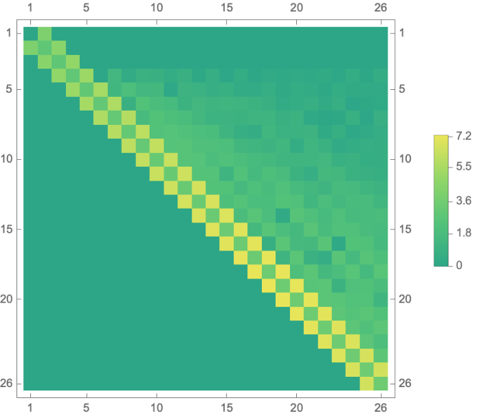
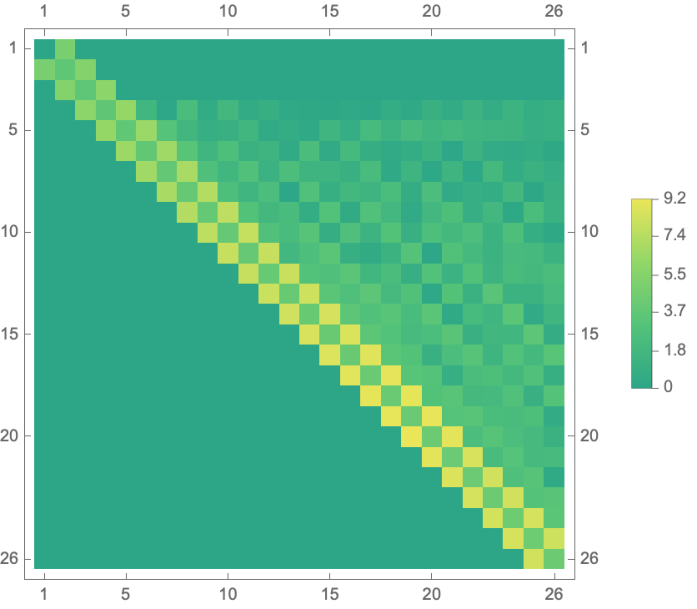
We numerically observe that $h_{n,n-1}\neq h_{n-1,n}$. In fact, their differences behave non-linearly with $n$ for both in integrable and chaotic limit (see Fig. 3 (c), (d)). Moreover, the other non-diagonal elements also do not vanish (except the first three rows) although their magnitude is far less compared to the primary of off-diagonal elements. In Fig. 4, we have shown the matrix elements in tridiagonal (for closed system) and the upper-Hessenberg form. The elements vary significantly with the increase of bulk dephasing parameter (see Appendix B). These two features are completely new for the Lindbladian and in sharp contrast with the usual Liouvillian which takes a tridiagonal form in Krylov basis. The purely imaginary diagonal entries $h_{n,n}$ are a clear reflection of non-Hermiticity in the case of open systems. When the magnitude of the diagonal entries is plotted with $n$ (see Fig. 5), they successfully capture the information about different non-Hermiticity parameters $\alpha$ and $\gamma$.^** * Note that the diagonal entries are zero for closed system, $\alpha=0,\,\gamma=0$. Hence, both the Lanczos algorithm and Arnoldi iteration give the same results in this case. However, when the growth of the magnitude of the diagonal entries for integrable and chaotic cases are compared, they are indistinguishable (see Fig. 6 (a), (b)).

More on the form of the Lindbladian matrix: Here we would like to focus on the form of the Arnoldi matrix. Firstly, $h_{n,n-1}\neq h_{n-1,n}$ is just an artefact of the construction of the Arnoldi matrix. In the usual generalized Lanczos algorithm, since we anyway consider only two sets of coefficients $a_{n}$ and $b_{n}=h_{n-1,n}$, we ignore any possible differences between the row below the diagonals ($h_{n,n-1}$). In the Arnoldi matrix as well, if we look more closely, this difference comes only when there are nonzero coefficients in the upper triangular matrix other than the tridiagonal part (for example, $3$rd or $4$th off-diagonal rows and columns in Fig. 4 (c) and (d)). Hence the difference can be attributed to the presence of other matrix elements in the Arnoldi form. Effectively, this difference spreads in the other set of coefficients. It is worth mentioning that if one makes a systematic approximation of obtaining these small extra coefficients, then an effective tridiagonal form will reappear. For the moment, we ignore them (set them to zero) and we will get back to them in Appendix C.

1. 1.

   Real primary off-diagonal elements $(h_{n,n-1}$ and $h_{n-1,n})$: The coefficients $h_{n,n-1}$ and $h_{n-1,n}$ are the norms of vectors $u_{n}$ as explained in the algorithm. These norms will always be real numbers since even for a non-Hermitian vector $u_{n}$; the norm is defined as $\mathrm{Tr}(u_{n}^{\dagger}u_{n})$, which can only be a real positive number.

2. 2.

   Purely imaginary diagonal elements $(h_{n,n})$: Now that we know the $h_{n,n-1}$ or $b_{n}$-like elements are real, we might expect some complex numbers to show up in the diagonals. However, as we have seen in earlier sections these elements are purely imaginary. Then it is a valid question to ask why do not these coefficient have a real part. To address this issue, we note that in previous literature Albert_2014, the Lindbladian evolution has been studied in the form $e^{\tilde{\mathcal{L}_{o}}t}$. In these cases, the Lindbladian eigenvalues are found to always appear in real and complex conjugate pairs. The complex conjugate pair of eigenvalues result from the non-unitary evolution and are extremely crucial in characterizing the non-unitary evolution. Now for this to hold, the polynomial characteristics equation of the Lindbladian matrix $|\tilde{\mathcal{L}}_{o}-\lambda I|=0$ form must satisfy the complex conjugate root theorem croot, which says that only a polynomial equation with all real coefficients can have either real or complex conjugate pair as roots. Now, since we considered the evolution as $e^{i\mathcal{L}_{o}t}$, we simply have to multiply our tridiagonal matrix form (assuming the other terms are just the difference between $h_{n,n-1}$ and $h_{n-1,n}$) to $i$ and then look at the properties of the polynomial characteristics equation. This modified matrix will therefore have purely negative and real diagonals and purely imaginary $h_{n,n-1}$. The form of the matrix will be

   $$\tilde{\mathcal{L}_{o}}=i\mathcal{L}_{o}=\begin{pmatrix}-|h_{1,1}|&ih_{1,2}&0&\cdots&0\\ ih_{2,1}&-|h_{2,2}|&ih_{2,3}&\cdots&0\\ 0&ih_{3,2}&-|h_{3,3}|&ih_{3,4}&\cdots\\ \cdots&\cdots&ih_{4,3}&\cdots&\cdots\\ 0&\cdots&\cdots&\cdots&ih_{n-1,n}\\ 0&0&\cdots&ih_{n,n-1}&-|h_{n,n}|\\ \end{pmatrix}\,.$$

   (27)

   For this matrix, it can be shown that all the coefficients of the characteristics polynomial equation are real. On the other hand, the possibility of a real part in the diagonals of our $\mathcal{L}_{o}$ will result in an imaginary part in the diagonals of the modified $\tilde{\mathcal{L}_{o}}$ (of the form of $ih_{n,n}=-\mathrm{Im}[h_{n,n}]+i\mathrm{Re}[h_{n,n}]$). In that case, we find that inevitably the characteristics equation will have complex coefficients.^** * We thank Prashanth Raman for helping us in the sketch of this argument. Therefore, by the complex conjugate roots theorem, this can never give real and complex conjugate pairs of eigenvalues. We give more detailed arguments in the Appendix C. With these arguments, we can conclude that the upper Hessenberg form of the Lindbladian with alternating real and purely imaginary values is unique and necessary for producing proper eigenvalues. Hence, this particular nature of alternating diagonals will be independent of the choice of Hamiltonian and the choice of coupling, and hence they are generically true for dissipative quantum systems.

When the Krylov basis is explored completely, the Arnoldi coefficients hit zero. See Fig. 6 (c), (d). This has to be the case, as we have taken a finite-dimensional system. There are a couple of points to remember for the case of a fully explored Krylov basis. In Rabinovici:2020ryf, the authors found that for the integrable SYK model, the Krylov dimension is much smaller than the chaotic case. However, as argued in Rabinovici:2021qqt, this is not true for generic integrable cases where the Krylov space dimension appears to be the same for both integrable and chaotic cases. Due to the phenomenon dubbed the Krylov-space localization Rabinovici:2021qqt, the space is explored less efficiently when the integrable yet strongly interacting XXZ spin chain is analyzed. This localization results in the saturation of Krylov complexity for integrable XXZ chain at a lower value than the chaotic case and happens in the fully symmetry-reduced sector.^** * We thank Julian Sonner and the anonymous referee for pointing out these facts to us. In our case, we find the Krylov space dimensions for integrable and chaotic cases to be almost the same, which is in agreement with the results of Rabinovici:2021qqt. It is worth mentioning that we find many fluctuations for higher Arnoldi coefficients, which can be averaged for the $s$ number of preceding and following coefficients for a specific coefficient (see caption of Fig. 6 more details). After this fluctuation-averaging, the behavior of the Arnoldi coefficients becomes much smoother, and one can observe the full exploration of the Krylov basis much more clearly. Yet, we can see that for integrable systems, the coefficients fluctuate more rapidly than the chaotic ones, which, according to Rabinovici:2021qqt, can again be attributed to the Krylov space localization for the integrable case. However, the non-Hermitian effects tend to reduce it in both integrable and chaotic limits. At this stage, we do not have a clear understanding of it, and it requires further investigation.

Dissipation and decoherence are ubiquitous in nature; hence it is of primary interest to study the operator growth in such systems. Our results indicate that the Lanczos algorithm, while well-suited for Hermitian operators, breaks down if the superoperator becomes non-Hermitian, e.g., in the case of open system Lindbladian evolution. The idea of information scrambling under dissipation also becomes problematic since the coefficients never saturate and exhibit unbounded growth. With changing the coupling with the environment, the growth rate of Lanczos coefficients changes (as discussed in Appendix A), and different kinds of interactions can be distinguished. On the other hand, the Arnoldi iteration, when applied to a non-Hermitian system, distinguishes both integrable and chaotic regimes as well as different non-Hermiticity parameters. The norms $h_{n,n-1}$, analogous to $b_{n}$, distinguish the integrable and chaotic regimes, whereas the purely imaginary diagonal entries $h_{n,n}$ capture the information about the non-Hermiticity parameters.^** * The diagonal entries also appear in the state complexity picture (although real in that case), where Liouvillian is replaced by the Hamiltonian Balasubramanian:2022tpr; Caputa:2022eye. The Liouvillian takes an upper-Hessenberg form which is not symmetric in its elements, a clear contrasting feature of tridiagonal Liouvillian of a closed system. This work, therefore, clearly reflects the breakdown of the Hermitian methods in open systems and supports the application of non-Hermitian methods like Arnoldi iteration.

There are a few interesting questions that need to be understood. Firstly, it would be interesting to back the conclusions by studying other quantum mechanical, and field-theoretic models like open XXZ chain PhysRevX.10.021019 or open Sachdev-Ye-Kitaev model Sa:2021tdr; Kulkarni:2021gtt with corresponding Lindblad operators. One might test the validity of UOGH in open quantum field theory Baidya:2017eho, i.e., whether the asymptotic scaling of the primary off-diagonal Arnoldi coefficients is linear in $n$, similar to the Lanczos coefficients for the closed systems Dymarsky:2021bjq. The interesting question is, what is the asymptotic scaling of (imaginary) diagonal elements? From the numerical examples, we see that their saturation depends on the interaction with the environment. Do they have any description in terms of a Toda chain flow Dymarsky:2019elm? Further, the upper-Hessenberg form of the Lindbladian asks for the role of the other off-diagonal elements than the primary ones. Especially, the smallness of their magnitude seeks whether they can be potentially eliminated by using repeated re-orthogonalization Rabinovici:2020ryf. However, we do not have an analytic result at this stage and would like to return to this issue in the future.

Although here we have only restricted to the growth of Lanczos and Arnoldi coefficients which serves our purpose, it would be interesting to compute Krylov complexity in such cases where the comparison with circuit complexity on open systems Bhattacharyya:2021fii could be possible. The primary obstacle is to ensure the conservation of probability on the Krylov basis, which might be lost, and show decay over time. This is potentially due to the presence of purely imaginary non-zero diagonal elements, even if they are small compared to the primary off-diagonal elements. One practical way could be to implement by bi-orthogonalizing the Lanczos algorithm Gruning; bilan, which will render the Lindbladian in pure tridiagonal form with different sets of coefficients.^** * We thank Xiangyu Cao for discussions on this point. Computing complexity, in such cases, could be practically possible without encountering significant numerical errors.

Our analysis opens up possibilities for the exploration of a vast field of non-Hermitian Hamiltonians, especially with having the PT-symmetry Bender:1998ke; Bender:2007nj, which has gained significant importance in recent experiments Ruter2010; feng; Assawaworrarit2017. By the balanced gain and loss mechanism, the closed PT symmetric system can be described by an open system dynamics such that the evolution of density matrix reads 10.21468/SciPostPhys.9.4.052; PhysRevA.105.022219; broody; Cornelius:2021ccu

$\displaystyle\dot{\rho}=-i\big(H_{\mathrm{eff}}\rho-\rho H_{\mathrm{eff}}^{\dagger}\big),~~~~H_{\mathrm{eff}}=H-\frac{i}{2}\sum_{i}L_{i}^{\dagger}L_{i}\,,$

where $H_{\mathrm{eff}}$ is the effective non-Hermitian Hamiltonian made up from the Hermitian Hamiltonian $H$ and the Lindblad operators $L_{i}$. In other words, this suggests that the operator growth in such systems will be controlled by $H_{\mathrm{eff}}$, which can efficiently obtained by implementing the Arnoldi iteration. We wish to report such issues in future studies.

We wish to thank Hugo A. Camargo, Xiangyu Cao, Pawel Caputa, Shajid Haque, Arnab Kundu, Sabyasachi Maulik, Jeff Murugan, Tatsuma Nishioka, Prashanth Raman, Sayak Ray, Shibaji Roy, Aninda Sinha, Masaki Tezuka, and Hendrik J.R. van Zyl for illuminating discussions and helpful comments on the draft. PN thanks Xiangyu Cao for ongoing collaboration on related topics and Tanay Pathak for implementing the numerical methods in Mathematica. PN would like to thank NITheCS and the University of Cape Town for the warm hospitality during the final stages of the work, where parts of the results were presented. AB would like to thank the TP III division of the University of Würzburg, and the faculty of Physics, University of Warsaw, for hosting him during the final stages of the work. AB is supported by the Institute of Eminence endowed postdoctoral fellowship offered by the Indian Institute of Science. The work of PN is supported by the JSPS Grant-in-Aid for Transformative Research Areas (A) “Extreme Universe” No. 21H05190.

References

- (1) M. Serbyn, Z. Papić and D. A. Abanin, Local conservation laws and the structure of the many-body localized states, Phys. Rev. Lett. 111 (Sep, 2013) 127201, [1305.5554].
- (2) V. Ros, M. Müller and A. Scardicchio, Integrals of motion in the many-body localized phase, Nuclear Physics B 891 (2015) 420–465, [1406.2175].
- (3) A. Chandran, I. H. Kim, G. Vidal and D. A. Abanin, Constructing local integrals of motion in the many-body localized phase, Phys. Rev. B 91 (Feb, 2015) 085425, [1407.8480].
- (4) M. V. Berry, M. Tabor and J. M. Ziman, Level clustering in the regular spectrum, Proceedings of the Royal Society of London. A. Mathematical and Physical Sciences 356 (1977) 375–394.
- (5) E. P. Wigner, On the distribution of the roots of certain symmetric matrices, Annals of Mathematics 67 (1958) 325–327.
- (6) O. Bohigas, M. J. Giannoni and C. Schmit, Characterization of chaotic quantum spectra and universality of level fluctuation laws, Phys. Rev. Lett. 52 (Jan, 1984) 1–4.
- (7) A. Chenu, M. Beau, J. Cao and A. del Campo, Quantum simulation of generic many-body open system dynamics using classical noise, Phys. Rev. Lett. 118 (Apr, 2017) 140403, [1608.01317].
- (8) M. Beau, J. Kiukas, I. L. Egusquiza and A. del Campo, Nonexponential Quantum Decay under Environmental Decoherence, Phys. Rev. Lett. 119 (2017) 130401, [1706.06943].
- (9) A. Del Campo and T. Takayanagi, Decoherence in Conformal Field Theory, JHEP 02 (2020) 170, [1911.07861].
- (10) Z. Xu, A. Chenu, T. Prosen and A. del Campo, Thermofield dynamics: Quantum Chaos versus Decoherence, Phys. Rev. B 103 (2021) 064309, [2008.06444].
- (11) D. Braun, Dissipative Quantum Chaos and Decoherence. Springer Tracts in Modern Physics. Springer Berlin Heidelberg, 2003.
- (12) Z. Xu, L. P. García-Pintos, A. Chenu and A. del Campo, Extreme Decoherence and Quantum Chaos, Phys. Rev. Lett. 122 (2019) 014103, [1810.02319].
- (13) R. Grobe, F. Haake and H.-J. Sommers, Quantum distinction of regular and chaotic dissipative motion, Phys. Rev. Lett. 61 (Oct, 1988) 1899–1902.
- (14) J. Ginibre, Statistical ensembles of complex, quaternion, and real matrices, Journal of Mathematical Physics 6 (1965) 440–449.
- (15) G. Akemann, M. Kieburg, A. Mielke and T. Prosen, Universal signature from integrability to chaos in dissipative open quantum systems, Phys. Rev. Lett. 123 (Dec, 2019) 254101, [1910.03520].
- (16) R. Hamazaki, K. Kawabata, N. Kura and M. Ueda, Universality classes of non-hermitian random matrices, Phys. Rev. Research 2 (Jun, 2020) 023286, [1904.13082].
- (17) J. M. Deutsch, Quantum statistical mechanics in a closed system, Phys. Rev. A 43 (Feb, 1991) 2046–2049.
- (18) M. Srednicki, Chaos and quantum thermalization, Phys. Rev. E 50 (Aug, 1994) 888–901.
- (19) M. Rigol, V. Dunjko, V. Yurovsky and M. Olshanii, Relaxation in a completely integrable many-body quantum system: An ab initio study of the dynamics of the highly excited states of 1d lattice hard-core bosons, Phys. Rev. Lett. 98 (Feb, 2007) 050405, [cond-mat/0604476].
- (20) M. Rigol, V. Dunjko and M. Olshanii, Thermalization and its mechanism for generic isolated quantum systems, Nature 452 (apr, 2008) 854–858, [0708.1324].
- (21) D. E. Parker, X. Cao, A. Avdoshkin, T. Scaffidi and E. Altman, A Universal Operator Growth Hypothesis, Phys. Rev. X 9 (2019) 041017, [1812.08657].
- (22) A. Dymarsky and M. Smolkin, Krylov complexity in conformal field theory, Phys. Rev. D 104 (2021) L081702, [2104.09514].
- (23) B. Bhattacharjee, X. Cao, P. Nandy and T. Pathak, Krylov complexity in saddle-dominated scrambling, JHEP 05 (2022) 174, [2203.03534].
- (24) A. Avdoshkin and A. Dymarsky, Euclidean operator growth and quantum chaos, Phys. Rev. Res. 2 (2020) 043234, [1911.09672].
- (25) A. Dymarsky and A. Gorsky, Quantum chaos as delocalization in Krylov space, Phys. Rev. B 102 (2020) 085137, [1912.12227].
- (26) J. L. F. Barbón, E. Rabinovici, R. Shir and R. Sinha, On The Evolution Of Operator Complexity Beyond Scrambling, JHEP 10 (2019) 264, [1907.05393].
- (27) E. Rabinovici, A. Sánchez-Garrido, R. Shir and J. Sonner, Operator complexity: a journey to the edge of Krylov space, JHEP 06 (2021) 062, [2009.01862].
- (28) S.-K. Jian, B. Swingle and Z.-Y. Xian, Complexity growth of operators in the SYK model and in JT gravity, JHEP 03 (2021) 014, [2008.12274].
- (29) J. D. Noh, Operator growth in the transverse-field ising spin chain with integrability-breaking longitudinal field, Phys. Rev. E 104 (Sep, 2021) 034112, [2107.08287].
- (30) X. Cao, A statistical mechanism for operator growth, J. Phys. A 54 (2021) 144001, [2012.06544].
- (31) J. M. Magan and J. Simón, On operator growth and emergent Poincaré symmetries, JHEP 05 (2020) 071, [2002.03865].
- (32) E. Rabinovici, A. Sánchez-Garrido, R. Shir and J. Sonner, Krylov localization and suppression of complexity, JHEP 03 (2022) 211, [2112.12128].
- (33) D. J. Yates and A. Mitra, Strong and almost strong modes of Floquet spin chains in Krylov subspaces, Phys. Rev. B 104 (2021) 195121, [2105.13246].
- (34) D. J. Yates, A. G. Abanov and A. Mitra, Lifetime of almost strong edge-mode operators in one-dimensional, interacting, symmetry protected topological phases, Phys. Rev. Lett. 124 (May, 2020) 206803, [2002.00098].
- (35) D. J. Yates, A. G. Abanov and A. Mitra, Dynamics of almost strong edge modes in spin chains away from integrability, Phys. Rev. B 102 (Nov, 2020) 195419, [2009.00057].
- (36) J. Kim, J. Murugan, J. Olle and D. Rosa, Operator delocalization in quantum networks, Phys. Rev. A 105 (2022) L010201, [2109.05301].
- (37) P. Caputa and S. Datta, Operator growth in 2d CFT, JHEP 12 (2021) 188, [2110.10519].
- (38) F. B. Trigueros and C.-J. Lin, Krylov complexity of many-body localization: Operator localization in Krylov basis, SciPost Phys. 13 (2022) 037, [2112.04722].
- (39) P. Caputa, J. M. Magan and D. Patramanis, Geometry of Krylov complexity, Phys. Rev. Res. 4 (2022) 013041, [2109.03824].
- (40) D. Patramanis, Probing the entanglement of operator growth, PTEP 2022 (2022) 063A01, [2111.03424].
- (41) N. Hörnedal, N. Carabba, A. S. Matsoukas-Roubeas and A. del Campo, Ultimate Physical Limits to the Growth of Operator Complexity, Commun. Phys. 5 (2022) 207, [2202.05006].
- (42) R. Heveling, J. Wang and J. Gemmer, Numerically probing the universal operator growth hypothesis, Phys. Rev. E 106 (2022) 014152, [2203.00533].
- (43) A. Kar, L. Lamprou, M. Rozali and J. Sully, Random matrix theory for complexity growth and black hole interiors, JHEP 01 (2022) 016, [2106.02046].
- (44) W. Mück and Y. Yang, Krylov complexity and orthogonal polynomials, Nucl. Phys. B 984 (2022) 115948, [2205.12815].
- (45) A. Banerjee, A. Bhattacharyya, P. Drashni and S. Pawar, CFT to BMS: Complexity and OTOC, 2205.15338.
- (46) R. Heveling, J. Wang, C. Bartsch and J. Gemmer, Stability of Exponentially Damped Oscillations under Perturbations of the Mori-Chain, J. Phys. Comm. 6 (2022) 085009, [2204.06903].
- (47) B. Yoshida and N. Y. Yao, Disentangling Scrambling and Decoherence via Quantum Teleportation, Phys. Rev. X 9 (2019) 011006, [1803.10772].
- (48) V. Viswanath and G. Müller, The Recursion Method: Application to Many Body Dynamics. Lecture Notes in Physics Monographs. Springer Berlin Heidelberg, 1994.
- (49) I. Vakulchyk, I. Yusipov, M. Ivanchenko, S. Flach and S. Denisov, Signatures of many-body localization in steady states of open quantum systems, Phys. Rev. B 98 (Jul, 2018) 020202, [1709.08882].
- (50) H.-P. Breuer and F. Petruccione, The Theory of Open Quantum Systems. Oxford University Press, Oxford, 2007, 10.1093/acprof:oso/9780199213900.001.0001.
- (51) G. Lindblad, On the generators of quantum dynamical semigroups, Communications in Mathematical Physics 48 (Jun, 1976) 119–130.
- (52) V. Gorini, A. Kossakowski and E. C. G. Sudarshan, Completely positive dynamical semigroups of n‐level systems, Journal of Mathematical Physics 17 (1976) 821–825, [https://aip.scitation.org/doi/pdf/10.1063/1.522979].
- (53) D. A. Lidar, Lecture notes on the theory of open quantum systems, 1902.00967.
- (54) A. Pal and D. A. Huse, Many-body localization phase transition, Phys. Rev. B 82 (Nov, 2010) 174411, [1010.1992].
- (55) S. Sachdev, Quantum Phase Transitions. Cambridge University Press, 2 ed., 2011, 10.1017/CBO9780511973765.
- (56) M. C. Bañuls, J. I. Cirac and M. B. Hastings, Strong and weak thermalization of infinite nonintegrable quantum systems, Phys. Rev. Lett. 106 (Feb, 2011) 050405, [1007.3957].
- (57) D. A. Roberts, D. Stanford and L. Susskind, Localized shocks, JHEP 03 (2015) 051, [1409.8180].
- (58) M.-D. Choi, Completely positive linear maps on complex matrices, Linear Algebra and its Applications 10 (1975) 285–290.
- (59) A. Jamiołkowski, Linear transformations which preserve trace and positive semidefiniteness of operators, Reports on Mathematical Physics 3 (1972) 275–278.
- (60) M. Jiang, S. Luo and S. Fu, Channel-state duality, Phys. Rev. A 87 (Feb, 2013) 022310.
- (61) L. Sá, P. Ribeiro and T. Prosen, Complex spacing ratios: A signature of dissipative quantum chaos, Phys. Rev. X 10 (Apr, 2020) 021019, [1910.12784].
- (62) M. Am-Shallem, A. Levy, I. Schaefer and R. Kosloff, Three approaches for representing lindblad dynamics by a matrix-vector notation, 2015.
- (63) P. Zanardi and N. Anand, Information scrambling and chaos in open quantum systems, Phys. Rev. A 103 (Jun, 2021) 062214, [2012.13172].
- (64) F. Andreadakis, N. Anand and P. Zanardi, Scrambling of Algebras in Open Quantum Systems, 2206.02033.
- (65) W. E. Arnoldi, The principle of minimized iterations in the solution of the matrix eigenvalue problem, Quarterly of Applied Mathematics 9 (1951) 17–29.
- (66) R. B. Lehoucq and D. C. Sorensen, Deflation techniques for an implicitly restarted arnoldi iteration, SIAM J. Matrix Anal. Appl. 17 (oct, 1996) 789–821.
- (67) F. Minganti and D. Huybrechts, Arnoldi-Lindblad time evolution: Faster-than-the-clock algorithm for the spectrum of time-independent and Floquet open quantum systems, Quantum 6 (2022) 649, [2109.01648].
- (68) Y. Saad, Numerical Methods for Large Eigenvalue Problems. SIAM, Philadelphia, 2011.
- (69) P. Arbenz, Lecture notes: Numerical Methods for Solving Large Scale Eigenvalue Problems, 2018.
- (70) V. V. Albert and L. Jiang, Symmetries and conserved quantities in lindblad master equations, Phys. Rev. A 89 (Feb, 2014) 022118, [1310.1523].
- (71) “Complex conjugate root theorem - wikipedia page.” https://en.wikipedia.org/wiki/Complex_conjugate_root_theorem.
- (72) V. Balasubramanian, P. Caputa, J. M. Magan and Q. Wu, Quantum chaos and the complexity of spread of states, Phys. Rev. D 106 (2022) 046007, [2202.06957].
- (73) P. Caputa and S. Liu, Quantum complexity and topological phases of matter, 2205.05688.
- (74) L. Sá, P. Ribeiro and T. Prosen, Lindbladian dissipation of strongly-correlated quantum matter, Phys. Rev. Res. 4 (2022) L022068, [2112.12109].
- (75) A. Kulkarni, T. Numasawa and S. Ryu, Lindbladian dynamics of the Sachdev-Ye-Kitaev model, Phys. Rev. B 106 (2022) 075138, [2112.13489].
- (76) A. Baidya, C. Jana, R. Loganayagam and A. Rudra, Renormalization in open quantum field theory. Part I. Scalar field theory, JHEP 11 (2017) 204, [1704.08335].
- (77) A. Bhattacharyya, T. Hanif, S. S. Haque and M. K. Rahman, Complexity for an open quantum system, Phys. Rev. D 105 (2022) 046011, [2112.03955].
- (78) M. Grüning, A. Marini and X. Gonze, Implementation and testing of Lanczos-based algorithms for random-phase approximation eigenproblems, Computational materials science 50 (2011) 2148–2156, [1102.3909].
- (79) Z. Bai et al, Templates for the Solution of Algebraic Eigenvalue Problems: A Practical Guide. SIAM, Philadelphia, 2000.
- (80) C. M. Bender and S. Boettcher, Real spectra in non-Hermitian Hamiltonians having PT symmetry, Phys. Rev. Lett. 80 (1998) 5243–5246, [physics/9712001].
- (81) C. M. Bender, Making sense of non-Hermitian Hamiltonians, Rept. Prog. Phys. 70 (2007) 947, [hep-th/0703096].
- (82) C. E. Rüter, K. G. Makris, R. El-Ganainy, D. N. Christodoulides, M. Segev and D. Kip, Observation of parity–time symmetry in optics, Nature Physics 6 (Mar, 2010) 192–195.
- (83) L. Feng, Z. J. Wong, R.-M. Ma, Y. Wang and X. Zhang, Single-mode laser by parity-time symmetry breaking, Science 346 (2014) 972–975.
- (84) S. Assawaworrarit, X. Yu and S. Fan, Robust wireless power transfer using a nonlinear parity–time-symmetric circuit, Nature 546 (Jun, 2017) 387–390.
- (85) J. Huber, P. Kirton, S. Rotter and P. Rabl, Emergence of PT-symmetry breaking in open quantum systems, SciPost Phys. 9 (2020) 52, [2003.02265].
- (86) Y. Nakanishi and T. Sasamoto, phase transition in open quantum systems with lindblad dynamics, Phys. Rev. A 105 (Feb, 2022) 022219, [2104.07349].
- (87) D. C. Brody, PT symmetry and the evolution speed in open quantum systems, 2105.09853.
- (88) J. Cornelius, Z. Xu, A. Saxena, A. Chenu and A. del Campo, Spectral Filtering Induced by Non-Hermitian Evolution with Balanced Gain and Loss: Enhancing Quantum Chaos, Phys. Rev. Lett. 128 (2022) 190402, [2108.06784].
- (89) “Continuant (mathematics) - wikipedia page.” https://en.wikipedia.org/wiki/Continuant_(mathematics)#Generalizations.
- (90) B. Bhattacharjee, X. Cao, P. Nandy and T. Pathak, (to appear), .