跳到论文正文
W Papers独立论文阅读器 arXiv:2207.05344 论文正文 计算阅读时间 · 0%
引用这篇论文根据当前论文元数据生成,正式投稿前建议核对。


License: CC BY 4.0
arXiv:2207.05344v2 [eess.SP] 19 Jul 2022

Simultaneous Indoor and Outdoor 3D Localization with STAR-RIS-Assisted Millimeter Wave Systems

Jiguang He1, Aymen Fakhreddine1, and George C. Alexandropoulos1,2 Affiliation: 1Technology Innovation Institute, 9639 Masdar City, Abu Dhabi, United Arab Emirates Affiliation: 2Department of Informatics and Telecommunications, National and Kapodistrian University of Athens
Panepistimiopolis Ilissia, 15784 Athens, Greece
Affiliation: e-mails: {jiguang.he, aymen.fakhreddine}@tii.ae, alexandg@di.uoa.gr
Abstract

Simultaneously transmitting (refracting) and reflecting reconfigurable intelligent surfaces (STAR-RISs) have been recently identified to improve the spectrum/energy efficiency and extend the communication range. However, their potential for enhanced concurrent indoor and outdoor localization has not yet been explored. In this paper, we study the fundamental limits, i.e., the Cramér Rao lower bounds (CRLBs) via Fisher information analyses, on the three-dimensional (3D) localization performance with a STAR-RIS at millimeter wave frequencies. The effect of the power splitting between refraction and reflection at the STAR-RIS as well as the power allocation between the two mobile stations (MSs) are investigated. By maximizing the principal angle between the two subspaces corresponding to the STAR-RIS reflection and refraction matrices, we are able to find the optimal solutions for these simultaneous operations. We verify that high-accuracy 3D localization can be achieved for both indoor and outdoor MSs when the system parameters are well optimized.

Index Terms: 
Reconfigurable intelligent surface, STAR-RIS, 3D localization, principal angle, Cramér Rao bound.

I Introduction

Reconfigurable intelligent surfaces (RISs) have recently been introduced for improved energy efficiency (EE), spectrum efficiency (SE), localization accuracy, sensing capability, as well as network/physical-layer security [1, 2, 3, 4, 5]. The RIS, either being passive, active, or hybrid, is used to smartly control the radio propagation environment, by virtue of multi-function capabilities, e.g., reflection, refraction, diffraction, polarization, scattering, and even absorption [6, 1]. In the literature, the RIS is commonly used as an intelligent reflector, which breaks the well-known law of reflection [7], to mitigate the blockage and shadowing effect, and expand the communication coverage, especially for millimeter wave (mmWave) and Terahertz (THz) communications.

Recently, there appears another new type of RIS, termed as simultaneously transmitting and reflecting RIS (STAR-RIS) [8], which can be regarded as a promising bridge linking indoor and outdoor connectivity. Unlike the conventional RIS, the STAR-RIS can simultaneously realize two different functionalities, e.g., reflection and refraction. Namely, mobile stations (MSs) on both sides of the STAR-RIS, for instance, one is indoor and the other is outdoor, can be served by it at the same time. In addition, the two functionalities can also be realized in different manners, e.g., energy splitting, time switching, and model switching.

Even though the potential of traditional reflective RISs for radio localization has been studied in the literature [9, 10], we envision that the localization capability can be even further extended by the introduction of one or multiple STAR-RISs. With the aid of such a surfaces, an outdoor base station (BS) is capable of localizing an indoor user, in addition to an outdoor user, via uplink sounding reference signal (SRS) transmission, not only at sub-6GHz but also mmWave frequency bands. In this paper, we study the Cramér Rao lower bounds (CRLBs) for the intermediate channel parameter estimation based on the Fisher information analysis, and extend it to three-dimensional (3D) localization of one indoor and one outdoor MSs by virtue of the Jacobian matrix. We also examine the effect of the energy splitting between the two STAR-RIS functionalities and power allocation between the two MSs during SRS transmission. Besides, we find the optimal design of the STAR-RIS based on the CRLBs, which offers better performance than other alternative designs.

Notations: A bold lowercase letter 𝐚{\mathbf{a}} denotes a vector, and a bold capital letter 𝐀{\mathbf{A}} denotes a matrix. (⋅)𝖳(\cdot)^{\mathsf{T}} and (⋅)𝖧(\cdot)^{\mathsf{H}} denote the matrix or vector transpose and Hermitian transpose, respectively. (⋅)−1(\cdot)^{-1} denotes inverse of a matrix, tr⁡(⋅)\mathrm{tr}(\cdot) denotes the trace operator, diag⁡(𝐚)\mathrm{diag}({\mathbf{a}}) denotes a square diagonal matrix with the entries of 𝐚{\mathbf{a}} on its diagonal, 𝐀⊗𝐁{\mathbf{A}}\otimes{\mathbf{B}} and 𝐀⋄𝐁{\mathbf{A}}\diamond{\mathbf{B}} denote the Kronecker and Khatri-Rao products of 𝐀{\mathbf{A}} and 𝐁{\mathbf{B}}, respectively, 𝔼⁡[⋅]\mathbb{E}[\cdot] and var⁡(⋅)\mathrm{var}(\cdot) are the expectation and variance operators, 𝟏\mathbf{1} is the all-one vector, 𝐈M{\mathbf{I}}_{M} denotes the M×MM\times M identity matrix, j=−1j=\sqrt{-1}, and ∥⋅∥2\|\cdot\|_{2} denotes the Euclidean norm of a vector. [𝐚]i[{\mathbf{a}}]_{i}, [𝐀]i​j[{\mathbf{A}}]_{ij}, and [𝐀]i:j,i:j[{\mathbf{A}}]_{i:j,i:j} denote the iith element of 𝐚{\mathbf{a}}, the (i,j)(i,j)th element of 𝐀{\mathbf{A}}, and the submatrix of 𝐀{\mathbf{A}} formed by rows i,i+1,…,ji,i+1,\ldots,j and columns i,i+1,…,ji,i+1,\ldots,j. Finally, |⋅||\cdot| returns the absolute value of a complex number.

II System Model
Refer to caption
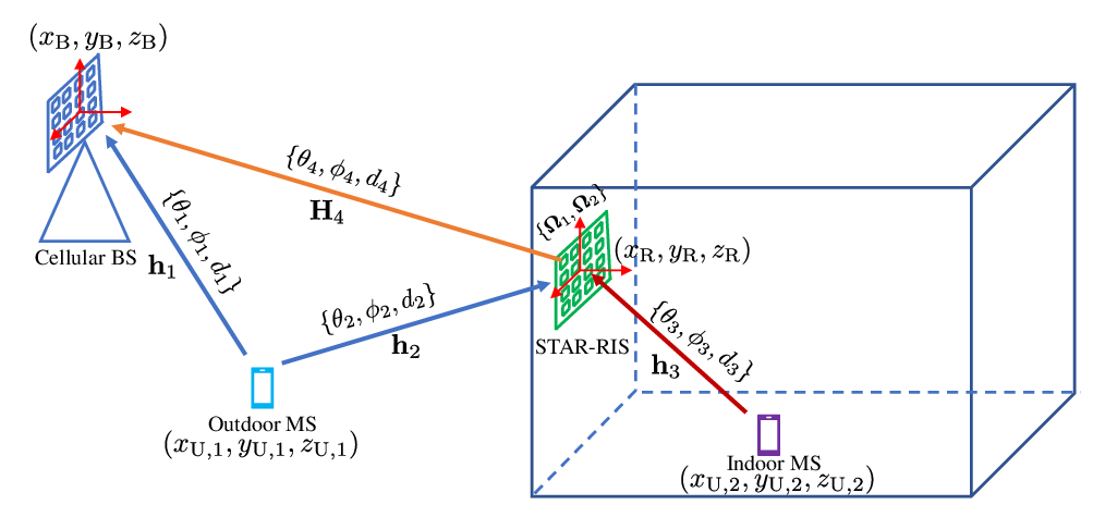
Fig. 1: The considered STAR-RIS-assisted mmWave MIMO systems for simultaneous indoor and outdoor 3D localization.

We consider a nearly-passive STAR-RIS-aided mmWave multiple-input multiple-output (MIMO) system, which consists of one multi-antenna BS, one multi-element STAR-RIS, one indoor MS, and one outdoor MS, which is intended for simultaneous indoor and outdoor 3D localization, as shown in Fig. 1. The BS and STAR-RIS are equipped with MM antennas and NN almost passive scattering elements, respectively, while each MS is equipped with a single antenna. Extension to multi-antenna MSs is feasible. Both the BS and STAR-RIS employ the uniform planar array (UPA) structure parallel to the x−zx-z plane. The STAR-RIS has two operation functionalities, i.e., reflection and refraction, which can be realized simultaneously.

II-A Channel Model

The system is assumed to operate in the mmWave frequency band and we consider the Saleh-Valenzuela parametric channel model to construct all four individual channels. The direct line-of-sight (LoS) channel between the outdoor MS and the MM-antenna cellular BS is denoted as 𝐡1∈ℂM×1{\mathbf{h}}_{1}\in\mathbb{C}^{M\times 1} and is mathematically expressed as follows:

𝐡1=e−j2πd1/λρ1​𝜶x​(θ1,ϕ1)⊗𝜶z​(ϕ1),{\mathbf{h}}_{1}=\frac{e^{-j2\pi d_{1}/\lambda}}{\sqrt{\rho_{1}}}\boldsymbol{\alpha}_{x}(\theta_{1},\phi_{1})\otimes\boldsymbol{\alpha}_{z}(\phi_{1}), (1)

where d1d_{1} (in meters) and ρ1\rho_{1} (for the sake of simplicity, we assume that ρ1=d12\rho_{1}=d_{1}^{2}) are the distance and path loss between the outdoor MS and BS, respectively, λ\lambda is the wavelength of the carrier frequency, θ1\theta_{1} and ϕ1\phi_{1} are the azimuth and elevation angles of arrival associated with 𝐡1{\mathbf{h}}_{1}, respectively.11 1 In fact, we can also consider the free-space path loss, which is modeled: ρ1=d12​fc2/108.755,\rho_{1}=d_{1}^{2}f_{c}^{2}/10^{8.755}, where fcf_{c} (in KHz) is the carrier frequency, defined as fc=cλf_{c}=\frac{c}{\lambda} with cc being the speed of light (3×1083\times 10^{8} m/s). Alternatively, the standard 3GPP urban micro (UMi) path loss model can be considered, according to which holds: ρ1=102.27​d13.67​fc2.6,\rho_{1}=10^{2.27}d_{1}^{3.67}f_{c}^{2.6}, where fcf_{c} needs to be included in GHz [11]. The steering vectors 𝜶x​(θ1,ϕ1)\boldsymbol{\alpha}_{x}(\theta_{1},\phi_{1}) and 𝜶z​(ϕ1)\boldsymbol{\alpha}_{z}(\phi_{1}) can be written as [12]:

𝜶x​(θ1,ϕ1)=\displaystyle\boldsymbol{\alpha}_{x}(\theta_{1},\phi_{1})= [e−j​2​π​dxλ​(Mx−12)​cos⁡(θ1)​sin⁡(ϕ1),\displaystyle\Big[e^{-j\frac{2\pi d_{x}}{\lambda}(\frac{M_{x}-1}{2})\cos(\theta_{1})\sin(\phi_{1})},
⋯,ej​2​π​dxλ​(Mx−12)​cos⁡(θ1)​sin⁡(ϕ1)]𝖳,\displaystyle\cdots,e^{j\frac{2\pi d_{x}}{\lambda}(\frac{M_{x}-1}{2})\cos(\theta_{1})\sin(\phi_{1})}\Big]^{\mathsf{T}}, (2)
𝜶z​(ϕ1)=\displaystyle\boldsymbol{\alpha}_{z}(\phi_{1})= [e−j​2​π​dzλ​(Mz−12)​cos⁡(ϕ1),\displaystyle\Big[e^{-j\frac{2\pi d_{z}}{\lambda}(\frac{M_{z}-1}{2})\cos(\phi_{1})},
⋯,ej​2​π​dzλ​(Mz−12)​cos⁡(ϕ1)]𝖳,\displaystyle\cdots,e^{j\frac{2\pi d_{z}}{\lambda}(\frac{M_{z}-1}{2})\cos(\phi_{1})}\Big]^{\mathsf{T}}, (3)

where M=Mx​MzM=M_{x}M_{z} with MxM_{x} and MzM_{z} being the number of horizontal and vertical BS antennas, respectively, and dxd_{x} and dzd_{z} denote their inter-element spacing in the horizontal and vertical axes, which were set as half-wavelength without loss of generality. Similarly, the other channels, e.g., 𝐡2∈ℂN×1{\mathbf{h}}_{2}\in\mathbb{C}^{N\times 1} and 𝐡3∈ℂN×1{\mathbf{h}}_{3}\in\mathbb{C}^{N\times 1}, can be presented in the same manner, as:

𝐡i=e−j2πdi/λρi​𝜶x​(θi,ϕi)⊗𝜶z​(ϕi),{\mathbf{h}}_{i}=\frac{e^{-j2\pi d_{i}/\lambda}}{\sqrt{\rho_{i}}}\boldsymbol{\alpha}_{x}(\theta_{i},\phi_{i})\otimes\boldsymbol{\alpha}_{z}(\phi_{i}), (4)

for i=2i=2 and 33, where N=Nx​NzN=N_{x}N_{z} is the number of STAR-RIS elements with NxN_{x} and NzN_{z} denoting the numbers in the horizontal and vertical axes, respectively. Note that the array response vectors 𝜶x​(⋅)\boldsymbol{\alpha}_{x}(\cdot) and 𝜶z​(⋅)\boldsymbol{\alpha}_{z}(\cdot) may have a different dimension compared to that in (1) but possess the same form. Finally, ρ2\rho_{2} and ρ3\rho_{3} follow the same assumption as ρ1\rho_{1}.

The wireless channel between the STAR-RIS and BS, i.e., 𝐇4∈ℂM×N{\mathbf{H}}_{4}\in\mathbb{C}^{M\times N}, is expressed as follows:

𝐇4=e−j2πd4/λρ4​𝜶x​(θ4,ϕ4)⊗𝜶z​(ϕ4)​(𝜶x​(θ4,ϕ4)⊗𝜶z​(ϕ4))𝖧,{\mathbf{H}}_{4}=\frac{e^{-j2\pi d_{4}/\lambda}}{\sqrt{\rho_{4}}}\boldsymbol{\alpha}_{x}(\theta_{4},\phi_{4})\otimes\boldsymbol{\alpha}_{z}(\phi_{4})(\boldsymbol{\alpha}_{x}(\theta_{4},\phi_{4})\otimes\boldsymbol{\alpha}_{z}(\phi_{4}))^{\mathsf{H}}, (5)

assuming that the two UPAs (i.e., one for the BS and the other for the STAR-RIS) are deployed in parallel without any biased orientation. Due to the wall in between the BS and the indoor MS, there does not exist a direct LoS path between them. The only path is the reflection route via the STAR-RIS. In this work, we consider only LoS paths in all the individual channels; the extension for the multipath scenario and for arbitrary orientations between the UPAs is left for future work.

II-B Geometric Relationship

The Cartesian coordinates of the BS and STAR-RIS as well as the outdoor and indoor MSs are 𝐩B=(xB,yB,zB)𝖳{\mathbf{p}}_{\text{B}}=(x_{\text{B}},y_{\text{B}},z_{\text{B}})^{\mathsf{T}}, 𝐩R=(xR,yR,zR)𝖳{\mathbf{p}}_{\text{R}}=(x_{\text{R}},y_{\text{R}},z_{\text{R}})^{\mathsf{T}}, 𝐩U,1=(xU,1,yU,1,zU,1)𝖳{\mathbf{p}}_{\text{U},1}=(x_{\text{U},1},y_{\text{U},1},z_{\text{U},1})^{\mathsf{T}}, and 𝐩U,2=(xU,2,yU,2,zU,2)𝖳{\mathbf{p}}_{\text{U},2}=(x_{\text{U},2},y_{\text{U},2},z_{\text{U},2})^{\mathsf{T}}, respectively. The relationship between the distances and a pair of Cartesian coordinates are listed below:

d1\displaystyle d_{1} =‖𝐩B−𝐩U,1‖2,\displaystyle=\|{\mathbf{p}}_{\text{B}}-{\mathbf{p}}_{\text{U},1}\|_{2}, (6)
di\displaystyle d_{i} =∥𝐩R−𝐩U,i−1∥2,fori=2,3,\displaystyle=\|{\mathbf{p}}_{\text{R}}-{\mathbf{p}}_{\text{U},i-1}\|_{2},\;\text{for}\;i=2,3, (7)
d4\displaystyle d_{4} =‖𝐩B−𝐩R‖2.\displaystyle=\|{\mathbf{p}}_{\text{B}}-{\mathbf{p}}_{\text{R}}\|_{2}. (8)

By introducing the three-element vector 𝝃i≜[cos⁡(θi)​cos⁡(ϕi),sin⁡(θi)​cos⁡(ϕi),sin⁡(ϕi)]𝖳\boldsymbol{\xi}_{i}\triangleq[\cos(\theta_{i})\cos(\phi_{i}),\sin(\theta_{i})\cos(\phi_{i}),\sin(\phi_{i})]^{\mathsf{T}} for i=1,2,3,4i=1,2,3,4, the geometric relationship between the angular parameters and the Cartesian coordinates of the nodes can be expressed as

𝐩R\displaystyle{\mathbf{p}}_{\text{R}} =𝐩B+d4​𝝃4,\displaystyle={\mathbf{p}}_{\text{B}}+d_{4}\boldsymbol{\xi}_{4}, (9)
𝐩U,1\displaystyle{\mathbf{p}}_{\text{U},1} =𝐩B+d1​𝝃1=𝐩R+d2​𝝃2,\displaystyle={\mathbf{p}}_{\text{B}}+d_{1}\boldsymbol{\xi}_{1}={\mathbf{p}}_{\text{R}}+d_{2}\boldsymbol{\xi}_{2}, (10)
𝐩U,2\displaystyle{\mathbf{p}}_{\text{U},2} =𝐩R+d3​𝝃3.\displaystyle={\mathbf{p}}_{\text{R}}+d_{3}\boldsymbol{\xi}_{3}. (11)

II-C Signal Model

Recall that the STAR-RIS has two operation functionalities, i.e., reflection and refraction. Two separate series of phase shifters are leveraged for controlling them, so each one is represented by a phase control matrix, i.e., 𝛀1\boldsymbol{\Omega}_{1} for controlling refraction and 𝛀2\boldsymbol{\Omega}_{2} for controlling reflection. 𝛀1\boldsymbol{\Omega}_{1} and 𝛀2\boldsymbol{\Omega}_{2} are diagonal matrices with each diagonal element satisfying the unit-modulus constraints, e.g., |[𝛀1]j​j|=|[𝛀2]j​j|=1|[\boldsymbol{\Omega}_{1}]_{jj}|=|[\boldsymbol{\Omega}_{2}]_{jj}|=1, ∀j=1,2,…,N\forall j=1,2,\ldots,N. We consider the 3D localization via the uplink transmission, where the two users send SRSs towards the BS simultaneously. The received signal during the kkth time slot, for k=1,2,…,Kk=1,2,\ldots,K, can be mathematically expressed as

𝐲k=𝐡1​x1,k+ϵ2​𝐇4​𝛀2,k​𝐡2​x1,k+ϵ1​𝐇4​𝛀1,k​𝐡3​x2,k+𝐧k,{\mathbf{y}}_{k}={\mathbf{h}}_{1}x_{1,k}+\epsilon_{2}{\mathbf{H}}_{4}\boldsymbol{\Omega}_{2,k}{\mathbf{h}}_{2}x_{1,k}+\epsilon_{1}{\mathbf{H}}_{4}\boldsymbol{\Omega}_{1,k}{\mathbf{h}}_{3}x_{2,k}+{\mathbf{n}}_{k}, (12)

where x1,kx_{1,k} is the SRS from the outdoor MS, x2,kx_{2,k} is the SRS from the indoor MS, as well as ϵ1\epsilon_{1} (for refraction) and ϵ2\epsilon_{2} (for reflection) are used to control the energy splitting for the two different operational modes of the STAR-RIS, satisfying the following condition: ϵ12+ϵ22=1\epsilon_{1}^{2}+\epsilon_{2}^{2}=1. The received signal at the BS is further corrupted by the white Gaussian noise 𝐧k{\mathbf{n}}_{k}, and each element of 𝐧k{\mathbf{n}}_{k} follows 𝒞​𝒩​(0,σ2)\mathcal{CN}(0,\sigma^{2}). During the kkth time slot, the refraction matrix 𝛀1,k\boldsymbol{\Omega}_{1,k} and the reflection matrix 𝛀2,k\boldsymbol{\Omega}_{2,k} are considered. In order to ensure good estimates, 𝛀1,k\boldsymbol{\Omega}_{1,k} and 𝛀2,k\boldsymbol{\Omega}_{2,k} vary from one time slot to another, i.e., 𝛀1,1≠𝛀1,2≠⋯≠𝛀1,K\boldsymbol{\Omega}_{1,1}\neq\boldsymbol{\Omega}_{1,2}\neq\cdots\neq\boldsymbol{\Omega}_{1,K}, and 𝛀2,1≠𝛀2,2≠⋯≠𝛀2,K\boldsymbol{\Omega}_{2,1}\neq\boldsymbol{\Omega}_{2,2}\neq\cdots\neq\boldsymbol{\Omega}_{2,K}. This refractive/reflective beam sweeping was verified through our numerical results on the STAR-RIS design in Section IV-C.

Based on the received signals across KK time slots, the BS estimates the Cartesian coordinates of both the indoor and outdoor users, enabling 3D localization. Without loss of generality, we assume that the sum power constraint is applied for each time slot, i.e., 𝔼⁡[|x1,k|2]+𝔼⁡[|x1,k|2]=P\mathbb{E}[|x_{1,k}|^{2}]+\mathbb{E}[|x_{1,k}|^{2}]=P, ∀k\forall k. The vector 𝐲k{\mathbf{y}}_{k} in (12) can be further expressed as

𝐲k=\displaystyle{\mathbf{y}}_{k}= 𝐡1​x1,k+ϵ2​𝐇4​diag​(𝐡2)​𝝎2,k​x1,k\displaystyle{\mathbf{h}}_{1}x_{1,k}+\epsilon_{2}{\mathbf{H}}_{4}\mathrm{diag}({\mathbf{h}}_{2})\boldsymbol{\omega}_{2,k}x_{1,k}
+ϵ1​𝐇4​diag​(𝐡3)​𝝎1,k​x2,k+𝐧k,\displaystyle+\epsilon_{1}{\mathbf{H}}_{4}\mathrm{diag}({\mathbf{h}}_{3})\boldsymbol{\omega}_{1,k}x_{2,k}+{\mathbf{n}}_{k}, (13)

where 𝛀1,k=diag⁡(𝝎1,k)\boldsymbol{\Omega}_{1,k}=\mathrm{diag}(\boldsymbol{\omega}_{1,k}) and 𝛀2,k=diag⁡(𝝎2,k)\boldsymbol{\Omega}_{2,k}=\mathrm{diag}(\boldsymbol{\omega}_{2,k}), ∀k\forall k. By stacking all 𝐲k{\mathbf{y}}_{k}’s column by column, we get the expression:

𝐘=\displaystyle{\mathbf{Y}}= η1​P​𝐡1​𝟏𝖳+η1​P​ϵ2​𝐇4​diag​(𝐡2)​𝛀¯2\displaystyle\eta_{1}\sqrt{P}{\mathbf{h}}_{1}\mathbf{1}^{\mathsf{T}}+\eta_{1}\sqrt{P}\epsilon_{2}{\mathbf{H}}_{4}\mathrm{diag}({\mathbf{h}}_{2})\bar{\boldsymbol{\Omega}}_{2}
+η2​P​ϵ1​𝐇4​diag​(𝐡3)​𝛀¯1+𝐍,\displaystyle+\eta_{2}\sqrt{P}\epsilon_{1}{\mathbf{H}}_{4}\mathrm{diag}({\mathbf{h}}_{3})\bar{\boldsymbol{\Omega}}_{1}+{\mathbf{N}}, (14)

where 𝟏\mathbf{1} denotes the KK-element all-one vector, 𝐘=[𝐲1,⋯,𝐲K]{\mathbf{Y}}=[{\mathbf{y}}_{1},\cdots,{\mathbf{y}}_{K}], 𝐍=[𝐧1,⋯,𝐧K]{\mathbf{N}}=[{\mathbf{n}}_{1},\cdots,{\mathbf{n}}_{K}], 𝛀¯1=[𝝎1,1,⋯,𝝎1,K]\bar{\boldsymbol{\Omega}}_{1}=[\boldsymbol{\omega}_{1,1},\cdots,\boldsymbol{\omega}_{1,K}], and 𝛀¯2=[𝝎2,1,⋯,𝝎2,K]\bar{\boldsymbol{\Omega}}_{2}=[\boldsymbol{\omega}_{2,1},\cdots,\boldsymbol{\omega}_{2,K}]. We have also set |x1,k|2=η12​P|x_{1,k}|^{2}=\eta_{1}^{2}P, |x2,k|2=η22​P|x_{2,k}|^{2}=\eta_{2}^{2}P, where η12+η22=1\eta_{1}^{2}+\eta_{2}^{2}=1. Applying vectorization to 𝐘{\mathbf{Y}} in (II-C), the following expression is deduced:

𝐲=\displaystyle{\mathbf{y}}= η1​P​(𝟏⊗𝐈M)​𝐡1+η1​P​ϵ2​(𝛀¯2𝖳⊗𝐈M)​(𝐈N⋄𝐇4)​𝐡2\displaystyle\eta_{1}\sqrt{P}(\mathbf{1}\otimes{\mathbf{I}}_{M}){\mathbf{h}}_{1}+\eta_{1}\sqrt{P}\epsilon_{2}(\bar{\boldsymbol{\Omega}}_{2}^{\mathsf{T}}\otimes{\mathbf{I}}_{M})({\mathbf{I}}_{N}\diamond{\mathbf{H}}_{4}){\mathbf{h}}_{2}
+η2​P​ϵ1​(𝛀¯1𝖳⊗𝐈M)​(𝐈N⋄𝐇4)​𝐡3+𝐧,\displaystyle+\eta_{2}\sqrt{P}\epsilon_{1}(\bar{\boldsymbol{\Omega}}_{1}^{\mathsf{T}}\otimes{\mathbf{I}}_{M})({\mathbf{I}}_{N}\diamond{\mathbf{H}}_{4}){\mathbf{h}}_{3}+{\mathbf{n}}, (15)

where 𝐲=vec⁡(𝐘){\mathbf{y}}=\mathrm{vec}({\mathbf{Y}}) and 𝐧=vec⁡(𝐍){\mathbf{n}}=\mathrm{vec}({\mathbf{N}}). We further introduce the following new notations to simplify the analyses that follows:

𝐀1\displaystyle{\mathbf{A}}_{1} =(𝟏⊗𝐈M),\displaystyle=(\mathbf{1}\otimes{\mathbf{I}}_{M}), (16)
𝐀2\displaystyle{\mathbf{A}}_{2} =(𝛀¯2𝖳⊗𝐈M)​(𝐈N⋄𝐇4),\displaystyle=(\bar{\boldsymbol{\Omega}}_{2}^{\mathsf{T}}\otimes{\mathbf{I}}_{M})({\mathbf{I}}_{N}\diamond{\mathbf{H}}_{4}), (17)
𝐀3\displaystyle{\mathbf{A}}_{3} =(𝛀¯1𝖳⊗𝐈M)​(𝐈N⋄𝐇4).\displaystyle=(\bar{\boldsymbol{\Omega}}_{1}^{\mathsf{T}}\otimes{\mathbf{I}}_{M})({\mathbf{I}}_{N}\diamond{\mathbf{H}}_{4}). (18)

To this end, expression in (II-C) can be re-written as:

𝐲=P​η1​𝐀1​𝐡1+P​η1​ϵ2​𝐀2​𝐡2+P​η2​ϵ1​𝐀3​𝐡3+𝐧.{\mathbf{y}}=\sqrt{P}\eta_{1}{\mathbf{A}}_{1}{\mathbf{h}}_{1}+\sqrt{P}\eta_{1}\epsilon_{2}{\mathbf{A}}_{2}{\mathbf{h}}_{2}+\sqrt{P}\eta_{2}\epsilon_{1}{\mathbf{A}}_{3}{\mathbf{h}}_{3}+{\mathbf{n}}. (19)

Upon the STAR-RIS deployment, we assume that the BS knows the exact/precise location of the STAR-RIS. Thus, we assume that the BS has exact information on 𝐇4{\mathbf{H}}_{4} in terms of the parameters θ4\theta_{4}, ϕ4\phi_{4}, and d4d_{4}.22 2 The assumption needs to be further relaxed since perfect information is usually infeasible in practice. Therefore, 𝐀1{\mathbf{A}}_{1}, 𝐀2{\mathbf{A}}_{2}, and 𝐀3{\mathbf{A}}_{3} in (19) are known measurement matrices to the BS (the BS also knows the refractive/reflective phase configurations due to its interaction with the STAR-RIS controller).

III Cramér Rao Lower Bound Analyses

In this section, we will provide the CRLBs on the estimation of the intermediate channel parameters, followed by the 3D Cartesian coordinates’ estimation. We also present the refractive/reflective optimization of the STAR-RIS for the indoor/outdoor localization objective.

III-A Estimation of Channel Parameters

The channel parameters to be estimated are those included in 𝐡1{\mathbf{h}}_{1}, 𝐡2{\mathbf{h}}_{2}, and 𝐡3{\mathbf{h}}_{3}, i.e., the nine-tuple 𝝂≜[θ1,ϕ1,d1,θ2,ϕ2,d2,θ3,ϕ3,d3]𝖳\boldsymbol{\nu}\triangleq[\theta_{1},\phi_{1},d_{1},\theta_{2},\phi_{2},d_{2},\theta_{3},\phi_{3},d_{3}]^{\mathsf{T}}. Since the additive noise is complex Gaussian distributed, by introducing 𝝁⁡(𝝂)≜η1​𝐀1​𝐡1+η1​ϵ2​𝐀2​𝐡2+η2​ϵ1​𝐀3​𝐡3\boldsymbol{\mu}(\boldsymbol{\nu})\triangleq\eta_{1}{\mathbf{A}}_{1}{\mathbf{h}}_{1}+\eta_{1}\epsilon_{2}{\mathbf{A}}_{2}{\mathbf{h}}_{2}+\eta_{2}\epsilon_{1}{\mathbf{A}}_{3}{\mathbf{h}}_{3} for (19), the Fisher information matrix for 𝝂\boldsymbol{\nu} is obtained as:

[𝐉⁡(𝝂)]i,j=Pσ2​ℜ⁡{∂𝝁𝖧∂νi​∂𝝁∂νj}.[{\mathbf{J}}(\boldsymbol{\nu})]_{i,j}=\frac{P}{\sigma^{2}}\Re\Big\{\frac{\partial\boldsymbol{\mu}^{\mathsf{H}}}{\partial\nu_{i}}\frac{\partial\boldsymbol{\mu}}{\partial\nu_{j}}\Big\}. (20)

The detailed information on the partial derivatives in (20) related to parameters in 𝐡1{\mathbf{h}}_{1}, 𝐡2{\mathbf{h}}_{2}, and 𝐡3{\mathbf{h}}_{3} is provided below:

∂𝝁∂θ1\displaystyle\frac{\partial\boldsymbol{\mu}}{\partial\theta_{1}} =η1​𝐀1​(𝐃11⊗𝐈Mx)​𝐡1,\displaystyle=\eta_{1}{\mathbf{A}}_{1}({\mathbf{D}}_{11}\otimes{\mathbf{I}}_{M_{x}}){\mathbf{h}}_{1}, (21)
∂𝝁∂ϕ1\displaystyle\frac{\partial\boldsymbol{\mu}}{\partial\phi_{1}} =η1​𝐀1​(𝐃12⊗𝐈Mx)​𝐡1+η1​𝐀1​(𝐈Mz⊗𝐃13)​𝐡1,\displaystyle=\eta_{1}{\mathbf{A}}_{1}({\mathbf{D}}_{12}\otimes{\mathbf{I}}_{M_{x}}){\mathbf{h}}_{1}+\eta_{1}{\mathbf{A}}_{1}({\mathbf{I}}_{M_{z}}\otimes{\mathbf{D}}_{13}){\mathbf{h}}_{1},
=η1​𝐀1​(𝐃12⊗𝐈Mx+𝐈Mz⊗𝐃13)​𝐡1,\displaystyle=\eta_{1}{\mathbf{A}}_{1}({\mathbf{D}}_{12}\otimes{\mathbf{I}}_{M_{x}}+{\mathbf{I}}_{M_{z}}\otimes{\mathbf{D}}_{13}){\mathbf{h}}_{1}, (22)
∂𝝁∂d1\displaystyle\frac{\partial\boldsymbol{\mu}}{\partial d_{1}} =η1​−j2πd1/λ−1d1​𝐀1​𝐡1,\displaystyle=\eta_{1}\frac{-j2\pi d_{1}/\lambda-1}{d_{1}}{\mathbf{A}}_{1}{\mathbf{h}}_{1}, (23)
∂𝝁∂θ2\displaystyle\frac{\partial\boldsymbol{\mu}}{\partial\theta_{2}} =η1​ϵ2​𝐀2​(𝐃21⊗𝐈Nx)​𝐡2,\displaystyle=\eta_{1}\epsilon_{2}{\mathbf{A}}_{2}({\mathbf{D}}_{21}\otimes{\mathbf{I}}_{N_{x}}){\mathbf{h}}_{2}, (24)
∂𝝁∂ϕ2\displaystyle\frac{\partial\boldsymbol{\mu}}{\partial\phi_{2}} =η1​ϵ2​𝐀2​(𝐃22⊗𝐈Nx)​𝐡2+η1​ϵ2​𝐀2​(𝐈Nz⊗𝐃23)​𝐡2,\displaystyle=\eta_{1}\epsilon_{2}{\mathbf{A}}_{2}({\mathbf{D}}_{22}\otimes{\mathbf{I}}_{N_{x}}){\mathbf{h}}_{2}+\eta_{1}\epsilon_{2}{\mathbf{A}}_{2}({\mathbf{I}}_{N_{z}}\otimes{\mathbf{D}}_{23}){\mathbf{h}}_{2},
=η1​ϵ2​𝐀2​(𝐃22⊗𝐈Nx+𝐈Nz⊗𝐃23)​𝐡2,\displaystyle=\eta_{1}\epsilon_{2}{\mathbf{A}}_{2}({\mathbf{D}}_{22}\otimes{\mathbf{I}}_{N_{x}}+{\mathbf{I}}_{N_{z}}\otimes{\mathbf{D}}_{23}){\mathbf{h}}_{2}, (25)
∂𝝁∂d2\displaystyle\frac{\partial\boldsymbol{\mu}}{\partial d_{2}} =η1​ϵ2​−j2πd2/λ−1d2​𝐀2​𝐡2,\displaystyle=\eta_{1}\epsilon_{2}\frac{-j2\pi d_{2}/\lambda-1}{d_{2}}{\mathbf{A}}_{2}{\mathbf{h}}_{2}, (26)
∂𝝁∂θ3\displaystyle\frac{\partial\boldsymbol{\mu}}{\partial\theta_{3}} =η2​ϵ1​𝐀3​(𝐃31⊗𝐈Nx)​𝐡3,\displaystyle=\eta_{2}\epsilon_{1}{\mathbf{A}}_{3}({\mathbf{D}}_{31}\otimes{\mathbf{I}}_{N_{x}}){\mathbf{h}}_{3}, (27)
∂𝝁∂ϕ3\displaystyle\frac{\partial\boldsymbol{\mu}}{\partial\phi_{3}} =η2​ϵ1​𝐀3​(𝐃32⊗𝐈Nx)​𝐡3+η2​ϵ1​𝐀3​(𝐈Nz⊗𝐃33)​𝐡3,\displaystyle=\eta_{2}\epsilon_{1}{\mathbf{A}}_{3}({\mathbf{D}}_{32}\otimes{\mathbf{I}}_{N_{x}}){\mathbf{h}}_{3}+\eta_{2}\epsilon_{1}{\mathbf{A}}_{3}({\mathbf{I}}_{N_{z}}\otimes{\mathbf{D}}_{33}){\mathbf{h}}_{3},
=η2​ϵ1​𝐀3​(𝐃32⊗𝐈Nx+𝐈Nz⊗𝐃33)​𝐡3,\displaystyle=\eta_{2}\epsilon_{1}{\mathbf{A}}_{3}({\mathbf{D}}_{32}\otimes{\mathbf{I}}_{N_{x}}+{\mathbf{I}}_{N_{z}}\otimes{\mathbf{D}}_{33}){\mathbf{h}}_{3}, (28)
∂𝝁∂d3\displaystyle\frac{\partial\boldsymbol{\mu}}{\partial d_{3}} =η2​ϵ1​−j2πd3/λ−1d3​𝐀3​𝐡3,\displaystyle=\eta_{2}\epsilon_{1}\frac{-j2\pi d_{3}/\lambda-1}{d_{3}}{\mathbf{A}}_{3}{\mathbf{h}}_{3}, (29)

where we have used the following matrix definitions:

𝐃11=\displaystyle{\mathbf{D}}_{11}= diag([−jπ(−Mx−12)sin(θ1)sin(ϕ1),⋯,\displaystyle\mathrm{diag}\Big(\Big[-j\pi\Big(-\frac{M_{x}-1}{2}\Big)\sin(\theta_{1})\sin(\phi_{1}),\cdots,
−jπ(Mx−12)sin(θ1)sin(ϕ1)]),\displaystyle-j\pi\Big(\frac{M_{x}-1}{2}\Big)\sin(\theta_{1})\sin(\phi_{1})\Big]\Big), (30)
𝐃12=\displaystyle{\mathbf{D}}_{12}= diag⁡([j​π​(−Mx−12)​cos⁡(θ1)​cos⁡(ϕ1),⋯CLOSECLOSE,\displaystyle\mathrm{diag}\Big(\Big[j\pi\Big(-\frac{M_{x}-1}{2}\Big)\cos(\theta_{1})\cos(\phi_{1}),\cdots,
jπ(Mx−12)cos(θ1)cos(ϕ1)]),\displaystyle j\pi\Big(\frac{M_{x}-1}{2}\Big)\cos(\theta_{1})\cos(\phi_{1})\Big]\Big), (31)
𝐃13\displaystyle{\mathbf{D}}_{13} =diag([−jπ(−Mx−12)sin(ϕ1),⋯,\displaystyle=\mathrm{diag}\Big(\Big[-j\pi\Big(-\frac{M_{x}-1}{2}\Big)\sin(\phi_{1}),\cdots,
−jπ(Mx−12)sin(ϕ1)]),\displaystyle-j\pi\Big(\frac{M_{x}-1}{2}\Big)\sin(\phi_{1})\Big]\Big), (32)
𝐃i​1=\displaystyle{\mathbf{D}}_{i1}= diag([−jπ(−Nx−12)sin(θi)sin(ϕi),⋯,\displaystyle\mathrm{diag}\Big(\Big[-j\pi\Big(-\frac{N_{x}-1}{2}\Big)\sin(\theta_{i})\sin(\phi_{i}),\cdots,
−jπ(Nx−12)sin(θi)sin(ϕi)]),fori=2,3,\displaystyle-j\pi\Big(\frac{N_{x}-1}{2}\Big)\sin(\theta_{i})\sin(\phi_{i})\Big]\Big),\;\text{for}\;i=2,3, (33)
𝐃i​2=\displaystyle{\mathbf{D}}_{i2}= diag⁡([j​π​(−Nx−12)​cos⁡(θi)​cos⁡(ϕi),⋯CLOSECLOSE,\displaystyle\mathrm{diag}\Big(\Big[j\pi\Big(-\frac{N_{x}-1}{2}\Big)\cos(\theta_{i})\cos(\phi_{i}),\cdots,
jπ(Nx−12)cos(θi)cos(ϕi)]),fori=2,3,\displaystyle j\pi\Big(\frac{N_{x}-1}{2}\Big)\cos(\theta_{i})\cos(\phi_{i})\Big]\Big),\;\text{for}\;i=2,3, (34)
𝐃i​3=\displaystyle{\mathbf{D}}_{i3}= diag([−jπ(−Nx−12)sin(ϕi),⋯,\displaystyle\mathrm{diag}\Big(\Big[-j\pi\Big(-\frac{N_{x}-1}{2}\Big)\sin(\phi_{i}),\cdots,
−jπ(Nx−12)sin(ϕi)]),fori=2,3,\displaystyle-j\pi\Big(\frac{N_{x}-1}{2}\Big)\sin(\phi_{i})\Big]\Big),\;\text{for}\;i=2,3, (35)

under the assumption of half-wavelength inter-element spacing for both the BS and the STAR-RIS UPAs.

For the above estimators of the channel parameters (unbiased 𝝂^​(𝐲)\hat{\boldsymbol{\nu}}({\mathbf{y}})), we can calculate the CRLB on the error covariance matrix as follows:

𝔼⁡{(𝝂−𝝂^​(𝐲))​(𝝂−𝝂^​(𝐲))𝖧}⪰𝐉−1​(𝝂),\mathbb{E}\{(\boldsymbol{\nu}-\hat{\boldsymbol{\nu}}({\mathbf{y}}))(\boldsymbol{\nu}-\hat{\boldsymbol{\nu}}({\mathbf{y}}))^{\mathsf{H}}\}\succeq{\mathbf{J}}^{-1}(\boldsymbol{\nu}), (36)

where the notation 𝐀⪰𝐁{\mathbf{A}}\succeq{\mathbf{B}} for square matrices 𝐀{\mathbf{A}} and 𝐁{\mathbf{B}} means 𝐚𝖧​𝐀𝐚≥𝐚𝖧​𝐁𝐚{\mathbf{a}}^{\mathsf{H}}{\mathbf{A}}{\mathbf{a}}\geq{\mathbf{a}}^{\mathsf{H}}{\mathbf{B}}{\mathbf{a}} for any valid vector 𝐚{\mathbf{a}}.

III-B Estimation of 3D Cartesian Coordinates

We are interested in estimating the 3D Cartesian coordinates of the indoor and outdoor MSs. Therefore, after estimating the channel parameters, we need to map them to 3D Cartesian coordinates, e.g., 𝜿=[xU,1,yU,1,zU,1,xU,2,yU,2,zU,2]𝖳\boldsymbol{\kappa}=[x_{\text{U},1},y_{\text{U},1},z_{\text{U},1},x_{\text{U},2},y_{\text{U},2},z_{\text{U},2}]^{\mathsf{T}}, based on the geometrical relationship among the BS, the STAR-RIS, and the two MSs. For the CRLB evaluation of 𝜿\boldsymbol{\kappa}, we resort to the Jacobian matrix 𝐓{\mathbf{T}}, which links the connection between the channel parameters 𝝂\boldsymbol{\nu} and the 3D Cartesian coordinates of the two MSs 𝜿\boldsymbol{\kappa}. Each (i,j)(i,j)th element of 𝐓{\mathbf{T}} is expressed as:

[𝐓]i​j=∂[𝝂]j∂[𝜿]i.[{\mathbf{T}}]_{ij}=\frac{\partial[\boldsymbol{\nu}]_{j}}{\partial[\boldsymbol{\kappa}]_{i}}. (37)

We provide the following derivatives for the calculation of the submatrix of the Jacobian matrix related to the outdoor MS:

∂θi/∂xU,1\displaystyle\partial\theta_{i}/\partial x_{\text{U},1} =−sin⁡(θi)di​cos⁡(ϕi),\displaystyle=-\frac{\sin(\theta_{i})}{d_{i}\cos(\phi_{i})}, (38)
∂θi/∂yU,1\displaystyle\partial\theta_{i}/\partial y_{\text{U},1} =cos⁡(θi)di​cos⁡(ϕi),\displaystyle=\frac{\cos(\theta_{i})}{d_{i}\cos(\phi_{i})}, (39)
∂θi/∂zU,1\displaystyle\partial\theta_{i}/\partial z_{\text{U},1} =0,\displaystyle=0, (40)
∂ϕi/∂xU,1\displaystyle\partial\phi_{i}/\partial x_{\text{U},1} =−cos⁡(θi)​sin⁡(ϕi)di,\displaystyle=-\frac{\cos(\theta_{i})\sin(\phi_{i})}{d_{i}}, (41)
∂ϕi/∂yU,1\displaystyle\partial\phi_{i}/\partial y_{\text{U},1} =−sin⁡(θi)​sin⁡(ϕi)di,\displaystyle=-\frac{\sin(\theta_{i})\sin(\phi_{i})}{d_{i}}, (42)
∂ϕi/∂zU,1\displaystyle\partial\phi_{i}/\partial z_{\text{U},1} =cos⁡(ϕi)di,\displaystyle=\frac{\cos(\phi_{i})}{d_{i}}, (43)
∂di/∂xU,1\displaystyle\partial d_{i}/\partial x_{\text{U},1} =cos⁡(θi)​cos⁡(ϕi),\displaystyle=\cos(\theta_{i})\cos(\phi_{i}), (44)
∂di/∂yU,1\displaystyle\partial d_{i}/\partial y_{\text{U},1} =sin⁡(θi)​cos⁡(ϕi),\displaystyle=\sin(\theta_{i})\cos(\phi_{i}), (45)
∂di/∂zU,1\displaystyle\partial d_{i}/\partial z_{\text{U},1} =sin⁡(ϕi),\displaystyle=\sin(\phi_{i}), (46)

for i=1i=1 and 22. The submatrix of 𝐓{\mathbf{T}} related to the indoor MS can be computed in the same manner. In addition, it can be easily seen that only the channel parameters {θ1,ϕ1,d1,θ2,ϕ2,d2}\{\theta_{1},\phi_{1},d_{1},\theta_{2},\phi_{2},d_{2}\} are related to the coordinates (xU,1,yU,1,zU,1)(x_{\text{U},1},y_{\text{U},1},z_{\text{U},1}) of the outdoor MS, and only the parameters {θ3,ϕ3,d3}\{\theta_{3},\phi_{3},d_{3}\} are related to the coordinates (xU,2,yU,2,zU,2)(x_{\text{U},2},y_{\text{U},2},z_{\text{U},2}) of the indoor MS, as concluded from (10) and (11). Therefore, the Jacobian matrix 𝐓{\mathbf{T}} has the following form:

𝐓=[𝐓1𝟎𝟎𝐓2],{\mathbf{T}}=\begin{bmatrix}{\mathbf{T}}_{1}&\mathbf{0}\\ \mathbf{0}&{\mathbf{T}}_{2}\end{bmatrix}, (47)

where the submatrix 𝐓1∈ℝ3×6{\mathbf{T}}_{1}\in\mathbb{R}^{3\times 6} consists of the partial derivatives from (38) to (46), and the submatrix 𝐓2∈ℝ3×3{\mathbf{T}}_{2}\in\mathbb{R}^{3\times 3} consists of the partial derivatives related to the indoor MS; this part is omitted here due to the space limitation.

The Fisher information of 𝜿\boldsymbol{\kappa} can be then expressed as [10]

𝐉⁡(𝜿)=𝐓𝐉⁡(𝝂)​𝐓𝖳.{\mathbf{J}}(\boldsymbol{\kappa})={\mathbf{T}}{\mathbf{J}}(\boldsymbol{\nu}){\mathbf{T}}^{\mathsf{T}}. (48)

Similar to (36), we have the inequality for the CLRB:

𝔼⁡{(𝜿−𝜿^​(𝐲))​(𝜿−𝜿^​(𝐲))𝖳}⪰𝐉−1​(𝜿).\mathbb{E}\{(\boldsymbol{\kappa}-\hat{\boldsymbol{\kappa}}({\mathbf{y}}))(\boldsymbol{\kappa}-\hat{\boldsymbol{\kappa}}({\mathbf{y}}))^{\mathsf{T}}\}\succeq{\mathbf{J}}^{-1}(\boldsymbol{\kappa}). (49)

The lower bounds on the root mean square error (RMSE) of the position estimation of the outdoor and indoor MSs are:

RMSEU,1=var⁡(𝐱^U,1)\displaystyle\text{RMSE}_{\text{U},1}=\sqrt{\mathrm{var}(\hat{{\mathbf{x}}}_{\text{U},1})} ≥tr{[𝐉−1(𝜿)]1:3,1:3},\displaystyle\geq\sqrt{\mathrm{tr}\{[{\mathbf{J}}^{-1}(\boldsymbol{\kappa})]_{1:3,1:3}\}}, (50)
RMSEU,2=var⁡(𝐱^U,2)\displaystyle\text{RMSE}_{\text{U},2}=\sqrt{\mathrm{var}(\hat{{\mathbf{x}}}_{\text{U},2})} ≥tr{[𝐉−1(𝜿)]4:6,4:6}.\displaystyle\geq\sqrt{\mathrm{tr}\{[{\mathbf{J}}^{-1}(\boldsymbol{\kappa})]_{4:6,4:6}\}}. (51)

III-C Localization-Optimal Design for the STAR-RIS

By introducing 𝐆1≜[∂𝝁∂θ1,∂𝝁∂ϕ1,∂𝝁∂d1,∂𝝁∂θ2,∂𝝁∂ϕ2,∂𝝁∂d2]{\mathbf{G}}_{1}\triangleq[\frac{\partial\boldsymbol{\mu}}{\partial\theta_{1}},\frac{\partial\boldsymbol{\mu}}{\partial\phi_{1}},\frac{\partial\boldsymbol{\mu}}{\partial d_{1}},\frac{\partial\boldsymbol{\mu}}{\partial\theta_{2}},\frac{\partial\boldsymbol{\mu}}{\partial\phi_{2}},\frac{\partial\boldsymbol{\mu}}{\partial d_{2}}], 𝐆^1≜𝐆1​𝐓1𝖧\hat{{\mathbf{G}}}_{1}\triangleq{\mathbf{G}}_{1}{\mathbf{T}}_{1}^{\mathsf{H}}, 𝐆2≜[∂𝝁∂θ3,∂𝝁∂ϕ3,∂𝝁∂d3]{\mathbf{G}}_{2}\triangleq[\frac{\partial\boldsymbol{\mu}}{\partial\theta_{3}},\frac{\partial\boldsymbol{\mu}}{\partial\phi_{3}},\frac{\partial\boldsymbol{\mu}}{\partial d_{3}}], and 𝐆^2≜𝐆2​𝐓2𝖧\hat{{\mathbf{G}}}_{2}\triangleq{\mathbf{G}}_{2}{\mathbf{T}}_{2}^{\mathsf{H}}, the expression of 𝐉−1​(𝜿){\mathbf{J}}^{-1}(\boldsymbol{\kappa}) in (36) can be expressed as [13, 14]

𝐉−1​(𝜿)=σ2P​[(𝐆^1𝖧​(𝐈−𝐏𝐆^2)​𝐆^1)−1∗∗(𝐆^2𝖧​(𝐈−𝐏𝐆^1)​𝐆^2)−1],{\mathbf{J}}^{-1}\!(\boldsymbol{\kappa})\!=\!\frac{\sigma^{2}}{P}\begin{bmatrix}(\hat{{\mathbf{G}}}_{1}^{\mathsf{H}}({\mathbf{I}}\!-\!{\mathbf{P}}_{\hat{{\mathbf{G}}}_{2}})\hat{{\mathbf{G}}}_{1})^{-1}&*\\ *&(\hat{{\mathbf{G}}}_{2}^{\mathsf{H}}({\mathbf{I}}\!-\!{\mathbf{P}}_{\hat{{\mathbf{G}}}_{1}})\hat{{\mathbf{G}}}_{2})^{-1}\end{bmatrix}\!\!, (52)

where 𝐏𝐆^i=𝐆^i​(𝐆^i𝖧​𝐆^i)−1​𝐆^i𝖧{\mathbf{P}}_{\hat{{\mathbf{G}}}_{i}}=\hat{{\mathbf{G}}}_{i}(\hat{{\mathbf{G}}}_{i}^{\mathsf{H}}\hat{{\mathbf{G}}}_{i})^{-1}\hat{{\mathbf{G}}}_{i}^{\mathsf{H}} is the orthogonal projection onto the column space of 𝐆^i\hat{{\mathbf{G}}}_{i} for i=1i=1 and 22.

In order to simplify the diagonal terms in (52), we rewrite 𝐆1{\mathbf{G}}_{1} and 𝐆2{\mathbf{G}}_{2} as 𝐆1=[η1​𝐀1​𝐇1,η1​ϵ2​𝐀2​𝐇2]{\mathbf{G}}_{1}=[\eta_{1}{\mathbf{A}}_{1}{\mathbf{H}}_{1},\;\eta_{1}\epsilon_{2}{\mathbf{A}}_{2}{\mathbf{H}}_{2}] and 𝐆2=η2​ϵ1​𝐀3​𝐇3{\mathbf{G}}_{2}=\eta_{2}\epsilon_{1}{\mathbf{A}}_{3}{\mathbf{H}}_{3}, where 𝐇1=[(𝐃11⊗𝐈Mx)​𝐡1,(𝐃12⊗𝐈Mx+𝐈Mz⊗𝐃13)​𝐡1,−j2πd1/λ−1d1​𝐡1]{\mathbf{H}}_{1}=[({\mathbf{D}}_{11}\otimes{\mathbf{I}}_{M_{x}}){\mathbf{h}}_{1},\;({\mathbf{D}}_{12}\otimes{\mathbf{I}}_{M_{x}}+{\mathbf{I}}_{M_{z}}\otimes{\mathbf{D}}_{13}){\mathbf{h}}_{1},\;\frac{-j2\pi d_{1}/\lambda-1}{d_{1}}{\mathbf{h}}_{1}], 𝐇2=[(𝐃21⊗𝐈Nx)​𝐡2,(𝐃22⊗𝐈Nx+𝐈Nz⊗𝐃23)​𝐡2,−j2πd2/λ−1d2​𝐡2]{\mathbf{H}}_{2}=[({\mathbf{D}}_{21}\otimes{\mathbf{I}}_{N_{x}}){\mathbf{h}}_{2},\;({\mathbf{D}}_{22}\otimes{\mathbf{I}}_{N_{x}}+{\mathbf{I}}_{N_{z}}\otimes{\mathbf{D}}_{23}){\mathbf{h}}_{2},\;\frac{-j2\pi d_{2}/\lambda-1}{d_{2}}{\mathbf{h}}_{2}], and 𝐇3=[(𝐃31⊗𝐈Nx)​𝐡3,(𝐃32⊗𝐈Nx+𝐈Nz⊗𝐃33)​𝐡3,−j2πd3/λ−1d3​𝐡3]{\mathbf{H}}_{3}=[({\mathbf{D}}_{31}\otimes{\mathbf{I}}_{N_{x}}){\mathbf{h}}_{3},\;({\mathbf{D}}_{32}\otimes{\mathbf{I}}_{N_{x}}+{\mathbf{I}}_{N_{z}}\otimes{\mathbf{D}}_{33}){\mathbf{h}}_{3},\;\frac{-j2\pi d_{3}/\lambda-1}{d_{3}}{\mathbf{h}}_{3}]. It can be seen that 𝐀2{\mathbf{A}}_{2} is a function of 𝛀¯2\bar{\boldsymbol{\Omega}}_{2} and 𝐀3{\mathbf{A}}_{3} is a function of 𝛀¯1\bar{\boldsymbol{\Omega}}_{1}, while 𝐀1{\mathbf{A}}_{1} is independent of 𝛀¯1\bar{\boldsymbol{\Omega}}_{1} and 𝛀¯2\bar{\boldsymbol{\Omega}}_{2}. By dividing 𝐓1{\mathbf{T}}_{1} into two submatrices, i.e., as 𝐓1=[𝐓~1∈ℝ3×3,𝐓¯1∈ℝ3×3]{\mathbf{T}}_{1}=[\tilde{{\mathbf{T}}}_{1}\in\mathbb{R}^{3\times 3},\bar{{\mathbf{T}}}_{1}\in\mathbb{R}^{3\times 3}], we can derive the expressions 𝐆^1=η1​𝐀1​𝐇1​𝐓~1𝖧+η1​ϵ2​𝐀2​𝐇2​𝐓¯1𝖧\hat{{\mathbf{G}}}_{1}=\eta_{1}{\mathbf{A}}_{1}{\mathbf{H}}_{1}\tilde{{\mathbf{T}}}_{1}^{\mathsf{H}}+\eta_{1}\epsilon_{2}{\mathbf{A}}_{2}{\mathbf{H}}_{2}\bar{{\mathbf{T}}}_{1}^{\mathsf{H}} and 𝐆^2=η2​ϵ1​𝐀3​𝐇3​𝐓2𝖧\hat{{\mathbf{G}}}_{2}=\eta_{2}\epsilon_{1}{\mathbf{A}}_{3}{\mathbf{H}}_{3}{\mathbf{T}}_{2}^{\mathsf{H}}.

For the sake of tractability for the STAR-RIS optimization (i.e., 𝛀¯1\bar{\boldsymbol{\Omega}}_{1} and 𝛀¯2\bar{\boldsymbol{\Omega}}_{2}), we maximize the principal angle (within [0,π/2][0,\pi/2]) between the subspaces of 𝐆^1\hat{{\mathbf{G}}}_{1} and 𝐆^2\hat{{\mathbf{G}}}_{2} by following [13]. The optimal solutions are founded when [𝟏,𝛀¯2𝖳][\mathbf{1},\bar{\boldsymbol{\Omega}}_{2}^{\mathsf{T}}] is orthogonal to 𝛀¯1𝖳\bar{\boldsymbol{\Omega}}_{1}^{\mathsf{T}}. In this regard, the largest principal angle, e.g., π/2\pi/2, is obtained [15]. The choices for the 𝛀¯1\bar{\boldsymbol{\Omega}}_{1} and 𝛀¯2\bar{\boldsymbol{\Omega}}_{2} can be the non-overlapping parts of a DFT or a Hadamard matrix.33 3 Hadamard matrices possess good properties, since they only contain {−1,1}\{-1,1\}. Therefore, only 11-bit quantization is needed for both the reflection and refraction matrices at the STAR-RIS. Note that we need to assume that K≥2​NK\geq 2N here in order to guarantee that both 𝛀¯1\bar{\boldsymbol{\Omega}}_{1} and 𝛀¯2\bar{\boldsymbol{\Omega}}_{2} are optimal.

IV Numerical Results

In this section’s numerical investigation, we have set the system parameters as follows: 𝐩B=(0,0,8)𝖳{\mathbf{p}}_{\text{B}}=(0,0,8)^{\mathsf{T}}, 𝐩R=(2,2,5)𝖳{\mathbf{p}}_{\text{R}}=(2,2,5)^{\mathsf{T}}, 𝐩U,1=(5,1,2)𝖳{\mathbf{p}}_{\text{U},1}=(5,1,2)^{\mathsf{T}}, and 𝐩U,2=(1,5,2)𝖳{\mathbf{p}}_{\text{U},2}=(1,5,2)^{\mathsf{T}}. The numbers of BS antennas, STAR-RIS elements, and SRSs from each MS were set as M=16M=16, N=64N=64, and K=128K=128. The signal-to-noise ratio (SNR) is defined as P/σ2P/\sigma^{2}.

IV-A Results on the Channel Parameters’ Estimation

We evaluate the estimation of the intermediate parameters with different setups for the STAR-RIS energy splitting coefficient ϵ1\epsilon_{1} and the power allocation coefficient η1\eta_{1}, i.e., ϵ1=η1=0.5\epsilon_{1}=\eta_{1}=\sqrt{0.5}, ϵ1=0.9,η1=0.5\epsilon_{1}=\sqrt{0.9},\eta_{1}=\sqrt{0.5}, and ϵ1=0.5,η1=0.9\epsilon_{1}=\sqrt{0.5},\eta_{1}=\sqrt{0.9}. The simulation results on estimation of θi\theta_{i}’s and did_{i}’s are shown in Figs. 2 and 3 in terms of the mean square error (MSE). Due to the similar estimation performance for θi\theta_{i}’s, the results for ϕi\phi_{i}’s are omitted here. From the simulation results, we can see that when ϵ1\epsilon_{1} increases with fixed η1\eta_{1}, better performance on the estimation of parameters in 𝐡3{\mathbf{h}}_{3} can be achieved. Meanwhile, the performance degrades for the parameter estimation in 𝐡1{\mathbf{h}}_{1} and 𝐡2{\mathbf{h}}_{2} when η1\eta_{1} decreases (less transmission power at the outdoor MS). Note that when fixing η1\eta_{1}, the performance for the parameter estimation in 𝐡1{\mathbf{h}}_{1} will not change with ϵ1\epsilon_{1}.

Refer to caption
Fig. 2: CRLB on the estimation of {θi}\{\theta_{i}\} for i=1,2i=1,2 and 33 with different pairs of ϵ1\epsilon_{1} and η1\eta_{1}.
Refer to caption
Fig. 3: CRLB on the estimation of {di}\{d_{i}\} for i=1,2i=1,2 and 33 with different pairs of ϵ1\epsilon_{1} and η1\eta_{1}.

IV-B CRLBs on 3D Localization

Based on the expressions (48) and (49), we can calculate the CRLBs for the estimation of the 3D Cartesian coordinates of the indoor and outdoor MSs. The simulation results are shown in Fig. 4 in terms of RMSE. The performance of 3D localization has been controlled by the two parameters ϵ1\epsilon_{1} and η1\eta_{1}. When ϵ1=η1=0.5\epsilon_{1}=\eta_{1}=\sqrt{0.5}, the performance gap between the two MSs’ position estimation is small. However, in the other two cases, the gap is obvious. In this sense, well-selected ϵ1\epsilon_{1} and η1\eta_{1} can satisfy the quality of services (QoSs) and user fairness for both MSs simultaneously.

Refer to caption
Fig. 4: CRLB on the estimation of the 3D Cartesian coordinates of the two MSs with different pairs of ϵ1\epsilon_{1} and η1\eta_{1}.

More comprehensive results on ϵ1\epsilon_{1} and η1\eta_{1} on the 3D localization are shown in Fig. 5. In general, a small ϵ1\epsilon_{1} and a large η1\eta_{1} offer poor performance for the indoor MS. On the contrary, a large ϵ1\epsilon_{1} and a small η1\eta_{1} results in poor performance for the outdoor MS. However, for most of the cases, where it holds η1,ϵ1>0.3\eta_{1},\epsilon_{1}>0.3, we can achieve promising 3D localization in term of the RMSE for both MSs.

Refer to caption
Fig. 5: The effect of η1\eta_{1} and ϵ1\epsilon_{1} on the 3D localization, when the SNR is fixed to 1515 dB.

IV-C Effect of the STAR-RIS Design

We evaluate the effect of the STAR-RIS design by considering three different cases: i) 𝛀¯1\bar{\boldsymbol{\Omega}}_{1} and 𝛀¯2\bar{\boldsymbol{\Omega}}_{2} are part of a DFT matrix; ii) 𝛀¯1\bar{\boldsymbol{\Omega}}_{1} and 𝛀¯2\bar{\boldsymbol{\Omega}}_{2} are part of a Hadamard matrix; and iii) the phases of 𝛀¯1\bar{\boldsymbol{\Omega}}_{1} and 𝛀¯2\bar{\boldsymbol{\Omega}}_{2} are randomly generated. The simulation results are shown in Fig. 6. We observe that the first two cases have the same performance and outperform the third one, since according to Section III-C they are optimal. The performance gain is not obvious due to the fact that, for large KK and NN, case iii) approximates the optimal solutions (i.e., the subspaces of 𝐆^1\hat{{\mathbf{G}}}_{1} and 𝐆^2\hat{{\mathbf{G}}}_{2} are nearly orthogonal).

Refer to caption
Fig. 6: The effect of the STAR-RIS design on the 3D localization.

V Conclusion and Future Work

In this paper, we studied the fundamental 3D localization performance limits of STAR-RIS-aided mmWave MIMO systems for simultaneously serving one indoor MS and one outdoor MS. We also investigated the effect of energy splitting at the STAR-RIS and the power allocation between the two MSs to offer some useful insights for practical implementations. Moreover, the optimal design of the STAR-RIS reflection and refraction configuration matrices was derived by maximizing the principal angle of two associated subspaces.

In the future, we will focus on the design of practical localization algorithms, which attain this paper’s theoretical performance limits. We will also extend the CRLB analysis to general multipath scenarios and consider arbitrary orientations between the UPAs of the BS and the STAR-RIS.

References

  • [1] C. Huang, A. Zappone, G. C. Alexandropoulos, M. Debbah, and C. Yuen, “Reconfigurable intelligent surfaces for energy efficiency in wireless communication,” IEEE Trans. Wireless Commun., vol. 18, no. 8, pp. 4157–4170, Aug. 2019.
  • [2] Q. Wu, S. Zhang, B. Zheng, C. You, and R. Zhang, “Intelligent reflecting surface aided wireless communications: A tutorial,” IEEE Trans. Commun., vol. 69, no. 5, pp. 3313–3351, May 2021.
  • [3] H. Wymeersch, J. He, B. Denis, A. Clemente, and M. Juntti, “Radio localization and mapping with reconfigurable intelligent surfaces: Challenges, opportunities, and research directions,” IEEE Veh. Technol. Mag., vol. 15, no. 4, pp. 52–61, Dec. 2020.
  • [4] J. Hu, H. Zhang, B. Di, L. Li, K. Bian, L. Song, Y. Li, Z. Han, and H. V. Poor, “Reconfigurable intelligent surface based RF sensing: Design, optimization, and implementation,” IEEE J. Sel. Areas Commun., vol. 38, no. 11, pp. 2700–2716, Nov. 2020.
  • [5] E. Calvanese Strinati, G. C. Alexandropoulos, H. Wymeersch, B. Denis, V. Sciancalepore, R. D’Errico, A. Clemente, D.-T. Phan-Huy, E. D. Carvalho, and P. Popovski, “Reconfigurable, intelligent, and sustainable wireless environments for 6G smart connectivity,” IEEE Commun. Mag., vol. 59, no. 10, pp. 99–105, Oct. 2021.
  • [6] M. Di Renzo, M. Debbah, D.-T. Phan-Huy, A. Zappone, M.-S. Alouini, C. Yuen, V. Sciancalepore, G. C. Alexandropoulos, J. Hoydis, H. Gacanin et al., “Smart radio environments empowered by reconfigurable AI meta-surfaces: An idea whose time has come,” EURASIP J. Wireless Commun. Netw., vol. 2019, no. 1, pp. 1–20, May 2019.
  • [7] G. C. Alexandropoulos, G. Lerosey, M. Debbah, and M. Fink, “Reconfigurable intelligent surfaces and metamaterials: The potential of wave propagation control for 6G wireless communications,” IEEE ComSoc TCCN Newsletter, vol. 6, no. 1, 2020.
  • [8] Y. Liu, X. Mu, J. Xu, R. Schober, Y. Hao, H. V. Poor, and L. Hanzo, “STAR: Simultaneous transmission and reflection for 360∘ coverage by intelligent surfaces,” IEEE Wireless Commun., vol. 28, no. 6, pp. 102–109, Dec. 2021.
  • [9] J. He, H. Wymeersch, L. Kong, O. Silvén, and M. Juntti, “Large intelligent surface for positioning in millimeter wave MIMO systems,” in Proc. IEEE VTC-Spring, 2020, pp. 1–5.
  • [10] A. Elzanaty, A. Guerra, F. Guidi, and M.-S. Alouini, “Reconfigurable intelligent surfaces for localization: Position and orientation error bounds,” IEEE Trans. Signal Process., vol. 69, Aug. 2021.
  • [11] M. R. Akdeniz, Y. Liu, M. K. Samimi, S. Sun, S. Rangan, T. S. Rappaport, and E. Erkip, “Millimeter wave channel modeling and cellular capacity evaluation,” IEEE J. Sel. Areas Commun., vol. 32, no. 6, pp. 1164–1179, Jun. 2014.
  • [12] Y. Tsai, L. Zheng, and X. Wang, “Millimeter-wave beamformed full-dimensional MIMO channel estimation based on atomic norm minimization,” IEEE Trans. Commun., vol. 66, no. 12, pp. 6150–6163, Dec. 2018.
  • [13] L. L. Scharf and L. T. McWhorter, “Geometry of the Cramer-Rao bound,” Signal Process., vol. 31, no. 3, pp. 301–311, Apr. 1993.
  • [14] P. Pakrooh, A. Pezeshki, L. L. Scharf, D. Cochran, and S. D. Howard, “Analysis of Fisher information and the Cramér–Rao bound for nonlinear parameter estimation after random compression,” IEEE Trans. Signal Process., vol. 63, no. 23, pp. 6423–6428, Dec. 2015.
  • [15] G. H. Golub and C. F. Van Loan, Matrix computations. JHU press, 2013.