Quench-Probe Setup as Analyzer of Fractionalized Entanglement Spreading
Abstract
We propose a novel spatially inhomogeneous setup for revealing quench-induced fractionalized excitations in entanglement dynamics. In this quench-probe setting, the region undergoing a quantum quench is tunnel-coupled to a static region, the probe. Subsequently, the time-dependent entanglement signatures of a tunable subset of excitations propagating to the probe are monitored by energy selectivity. We exemplify the power of this generic approach by identifying a unique dynamical signature associated with the presence of an isolated Majorana zero mode in the post-quench Hamiltonian. In this case excitations emitted from the topological part of the system give rise to a fractionalized jump of in the entanglement entropy of the probe. This dynamical effect is highly sensitive to the localized nature of the Majorana zero mode, but does not require the preparation of a topological initial state.
Introduction.— Identifying physical signatures to distinguish and understand phases of matter occurring in nature is a main objective of research in physics. Dynamical approaches probing a system far from thermal equilibrium have become increasingly important. In particular, quantum quenches, i.e. abrupt changes of parameters in the Hamiltonian, have enabled unprecedented insights into structure and dynamics of quantum matter, both in theory Gogolin and Eisert 2016; Polkovnikov et al. 2011; Essler and Fagotti 2016 and experiment Kinoshita et al. 2006; Gring et al. 2012; Cheneau et al. 2012; Langen et al. 2013; Bloch et al. 2008. A prominent example is provided by the prediction and observation of non-equilibrium topological invariants Hauke et al. 2014; Vajna and Dóra 2015; Budich and Heyl 2016; Goldman et al. 2016; Eckardt 2017; Cooper et al. 2019; Bermudez et al. 2009; Caio et al. 2015; Hu et al. 2016; Wang et al. 2017; Sun et al. 2018; Hu and Zhao 2020; McGinley and Cooper 2018; Fläschner et al. 2017; Marks et al. 2021 that probe topological properties of matter without requiring the preparation of a topological equilibrium state.
As a powerful and genuinely quantum-mechanical diagnostic tool, the time-evolution of entanglement has been widely investigated Gogolin and Eisert 2016; Calabrese et al. 2016; Essler and Fagotti 2016; Calabrese 2020, including dynamical signatures of topology such as protected crossings in the entanglement spectrum Gong and Ueda 2018; Pastori et al. 2020; Sayyad et al. 2021; Micallo et al. 2020; Mondal et al. 2022. In homogeneous integrable systems, the spreading of entanglement after a quench is closely related to the propagation of pairs of entangled quasiparticle excitations with opposite momenta Calabrese and Cardy 2005; Calabrese and Cardy 2016; Kim and Huse 2013; Calabrese 2020. For more complex scenarios, involving for example periodic spatial modulations Bastianello and Calabrese 2018 or open systems Alba and Carollo 2021; Maity et al. 2020, richer entanglement structures related to quench-induced excitations represent a frontier of ongoing research Alba and Heidrich-Meisner 2014; Alba 2018; Bertini et al. 2018a; Alba et al. 2019; Alba 2019; Bertini et al. 2017; Bertini et al. 2018b; Bastianello and Collura 2020.
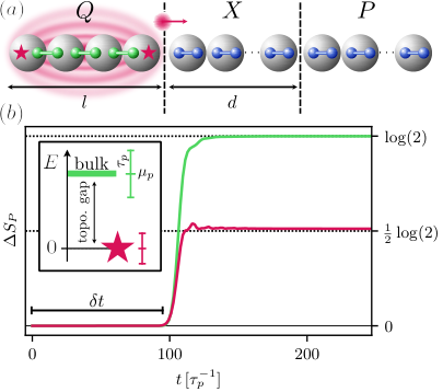
In this Letter, we propose a novel approach for the study of entanglement dynamics in complex systems to selectively analyze a subset of quench-induced excitations. This enables us to identify unique features in the spreading of entanglement, such as fractional jumps of the entanglement entropy (EE). We directly relate their presence to the existence of non-trivial eigenmodes in the post-quench Hamiltonian, e.g. topological localized modes. This remarkable capability stems from the hybrid nature of our proposed setup, sketched in Fig. 1(a), where only a part of the system () is quenched while the entanglement is measured in a different (static) region (), the two being coupled via a (static) separation layer (). This quench-probe approach provides a new perspective for the analysis of entanglement spreading in highly inhomogeneous systems, paving the way for novel observations that complement the study of (almost) homogeneous setups Calabrese and Cardy 2005; Calabrese and Cardy 2016; Eckardt 2017; Cooper et al. 2019; Alba and Calabrese 2017; Alba and Calabrese 2018; Giulio et al. 2019; Bastianello and Calabrese 2018; Bastianello and Collura 2020. Its energy selectivity – due to resonant coupling between regions and – is reminiscent of scanning tunneling spectroscopy.
As a specific case study, we use our approach to analyze the dynamics of the entanglement generated by a localized Majorana zero mode (MZM), hosted by a Kitaev chain (KC) Majorana 1937; Kitaev 2001; Alicea 2012. This leads us to the discovery of quantized jumps in the EE of the probe with fractional amplitude
| (1) |
The corresponding trace is provided by the red line in Fig. 1(b).
Such a fractional increase, associated with the fractional entropy of a single MZM Sela et al. 2019; Smirnov 2015; Silva et al. 2020, clearly differs from the conventional EE increase that originates from an ordinary fermionic mode [see the green line in Fig. 1(b)].
The quantization is robust with respect to parameter variations but highly sensitive to the hybridization of two MZMs.
These findings, representing a novel dynamical signature associated with a truly isolated MZM, are corroborated by the additional analysis of the mutual information (MI) shared between and Alba and Calabrese 2018; Maity et al. 2020; Mondal et al. 2022, which allows us to identify spurious contributions to the EE and highlight the fractional entanglement jumps.
Importantly, the observation of this toplogical signature only requires the post-quench Hamiltonian to be topological, while the system can be prepared in a trivial thermal state.
The topological nature (and robustness) of an isolated MZM is the origin of the fractional value of . Our setup is applicable to a variety of systems with particular entanglement spreading of either bulk or edge modes. Due to energy selective coupling, we are able to single out the contributions from a subset of modes, if they are separated in energy.
Hybrid quench-probe setup.—
We consider the system depicted in Fig. 1(a), consisting of the three parts labeled and . The first one, , is the one eventually undergoing a quantum quench. It is an -site KC described by the Hamiltonian
| (2) |
The operators create (annihilate) a spinless fermion at site , is the chemical potential, the nearest-neighbor hopping amplitude and the superconducting pairing amplitude. For simplicity, we consider those parameters to be non-negative real numbers. The KC features two different gapped phases, a trivial one for and a topological one for finite and . At the topological sweet spot (TSS), i.e. and , the analysis of in terms of Majorana operators reveals the presence of two completely isolated MZMs at the two open ends of the chain , depicted by red stars in Fig. 1(a). The bulk of the KC at the TSS is described by a flat band at finite energy . Deviations from the TSS (within the topological phase) imply an exponential leakage of the MZMs into the bulk, whose spectrum acquires then a finite bandwidth Alicea 2012. For simplicity, we illustrate the main features of our setup at the TSS. However, the observation of fractional EE is not limited to the TSS as we show below.
The remaining sites of the system are described by a tight-binding Hamiltonian
| (3) |
with chemical potential and hopping amplitude . The corresponding spectrum reads
| (4) |
The first sites, i.e. the ones between , form the separation layer , while the probe region consists of the remaining sites with . The presence of a finite allows us to consider regimes in which the probe region is exclusively affected by quench-induced excitations that propagate ballistically in the chain, filtering out possible contributions to the entanglement associated with the - interface. Regions and are connected via a standard tunneling Hamiltonian
| (5) |
with coupling strength .
It is particularly instructive to express fermions in terms of the corresponding Majorana operators. At the TSS, is an isolated MZM while , together with , belongs to an ordinary fermionic mode of the flat bulk band of the KC. Coupled Majorana operators belonging to the bulk of the KC are depicted by green circles in Fig. 1(a). By properly tuning the parameters of the system, it is thus possible to define two separated regimes. For the probe is exclusively coupled to the MZM at the right end of the topological KC. By contrast, for , the probe is coupled to the bulk band [Seethesupplementalmaterial; whichincludesRefs.\cite[cite]{\@@bibref{AuthorsPhrase1YearPhrase2}{Levy2019; Vidal et al. 2003; Calabrese and Cardy 2004; Holzhey et al. 1994; Islam et al. 2015; Kaufman et al. 2016; Lukin et al. 2019; Brydges2019}{\@@citephrase{(}}{\@@citephrase{)}}}.]supp. A sketch of this energy-selective coupling is provided in the inset of Fig. 1(b). The exploitation of energy and spatial sensitivity, together with the presence of a separation layer , differentiates our proposal from other quench-probe scenarios, such as the ones discussed in Calzona et al. 2017; Calzona et al. 2018; Ruggiero et al. 2021.
Quench procedure.— The quench of region consists in the abrupt change, at , of the parameters . We assume the system to be initially prepared in the ground state of the initial Hamiltonian . For , the time evolution of the system is instead controlled by the final Hamiltonian . With respect to , the state consists of several quasiparticle excitations, that are emitted in both directions from every site in the quenched region . Those counter-propagating quasiparticles are entangled between each other. Their motion is responsible for spreading of correlations and entanglement within the system, bounded by the Lieb-Robinson limit Lieb and Robinson 1972. For a wide range of homogeneous systems, these quasiparticles are produced in uncorrelated pairs, each one consisting of two entangled quasiparticles with opposite momenta Cazalilla et al. 2012; Schuricht and Essler 2012; Cazalilla 2006; De Nardis et al. 2014; Brockmann et al. 2014. The physics is richer in presence of interactions and/or inhomogeneities, which can lead to the presence of quasiparticle multiplets and non-trivial correlations Bertini et al. 2017; Bertini et al. 2018b; Bastianello and Calabrese 2018; Bastianello and Collura 2020. When is chosen in the topological regime, our system is spatially inhomogeneous due to the presence of a pair of isolated MZMs. This observation naturally raises the question whether the quasiparticles originating from the MZMs differ from the ones associated with the fermionic bulk of the KC. Our proposed quench-probe setup proves to be particularly effective in providing an affirmative answer to this question.
Entanglement dynamics.— The simplest way to analyze the entanglement properties of is to compute its EE, defined as
| (6) |
Here, is the reduced density matrix of the probe , whose spectrum can be calculated from the single-particle correlation matrix Peschel 2003; Peschel and Eisler 2009; Vidal et al. 2003. The time-dependent variation of the EE after a quench to the TSS is shown in Fig. 1(b), where we plot considering a selective coupling either to the isolated MZM (red line) or to the flat fermionic bulk band (green line). After a finite time delay , we observe jumps in the EE that eventually reach either the trivial quantized value (for the coupling to the bulk) or an anomalous fractional value (for the coupling to the MZM). Consistently with the quasiparticle picture, the time delay satisfies . It can be interpreted as the time-of-flight associated with the excitations, emitted from the last site of , that propagates through the sites of at the maximum group velocity [see Eq. (4)]. The lack of a steady linear increase of , typically observed in homogeneous systems Calabrese and Cardy 2005; Calabrese and Cardy 2016; Kim and Huse 2013, can be understood in terms of the vanishing group velocity in the bulk of the KC at the TSS. This effectively freezes all the quasiparticles emitted in with the only exception of the ones related to and , which are directly connected to via . Those quasiparticles are ultimately responsible for the quantized jumps discussed before.

To strengthen the connection between the anomalous fractional jump of the EE and the presence of an isolated MZM, we additionally compute the time-dependent mutual information (MI) shared between the probe and the quenched region . It is defined as
| (7) |
and quantifies the total amount of correlations between the two disjoint regions Alba and Calabrese 2018; Maity et al. 2020; Mondal et al. 2022, eliminating spurious contributions to coming from the separation layer and not from the quenched region . The increase of MI , where and for large sup, is plotted in the inset of Fig. 2 (dashed lines). It shares its main features with . In particular, when the probe is effectively coupled to the fermionic bulk of the KC (dashed lines), saturates at , indicating that and share a conventional fermionic mode sup. In contrast, when the probe is coupled to the isolated MZM (solid lines), the height of the increase is halved and saturates at . In the following, we carefully analyze the MZM case.
Anomalous quantization.— After a sufficiently long time and in the large limit 11 1 Note that the maximum time that can be actually studied is limited by the finite number of sites because we want to avoid a signal that stems from the reflections of quasiparticles at the right end of the region . The dependence of the signal on , the length of the region , is further discussed in the description of Fig. 4., shows a high degree of quantization and robustness. Indeed, as long as the probe is gapless and the initial Hamiltonian features a large trivial gap (such that regions and are initially decoupled), the MI saturates at without the need of fine-tuning, as shown by the extended white area in Fig. 3. Likewise, no fine-tuning of the tunnel coupling between and is necessary to produce the anomalous quantization signature, as long as it is comparable to sup. This anomalous quantization is robust against finite temperature effects and deviations of from the TSS, as can be seen from the large white area in Fig. 2. Away from the TSS, two main effects matter: (i) hybridization of MZMs and (ii) finite band-width of the fermionic bulk band. Related to point (i), the hybridization of the MZMs disturbs the saturation of the EE at the fractional value of log(2)/2. This makes sense because hybridized MZMs become regular fermions. If the region Q is, however, chosen long enough such that the hybridization between the MZMs is weak, then the fractional EE can be observed, see Fig.2. Related to point (ii), as long as the MZMs are energetically decoupled from the bulk, our quench-probe setup allows to isolate their contribution to the EE by energy selectivity.
As for the robustness at finite temperature, we show that the quantization of the MI is retained even when the system is initialized in a thermal trivial state of at finite temperature , as long as the latter remains smaller than the topological gap sup.

Non-equilibrium dynamics.— Our quench-probe setup features another useful knob, i.e. the size of region , which can significantly enrich the analysis of the post-quench entanglement dynamics. Indeed, a careful study of as a function of (plotted in Fig. 4) reveals the coexistence of a fixed and a propagating component of the correlations contributing to the MI. Let us explain this point by carefully inspecting Fig. 4, from right to left. If the probe region is too far away from , the quench-induced excitations have not yet reached and the MI is basically zero. This explains the large triangular gray area in Fig. 4, which is bounded by the Lieb-Robinson limit (black dashed line) 22 2 The small deviations from , which can be observed below the dashed line for small , are a consequence of the non-local nature of the MI.. To the left of the Lieb-Robinson line, the MI increases as the probe includes an increasing number of sites entangled with (orange region). The MI reaches close to the red-dotted line, which we attribute to the propagation of excitations of finite but smaller group velocity than . To the left of the red-dotted line, the MI features a plateau around the anomalous quantized value of (white region), the regime described in the previous paragraphs. For small , i.e. when the probe region starts to include sites close to the - interface, the MI increases again and displays values above (blue region). Interestingly, the correlations responsible for this additional increase of MI do not propagate within the probe, as shown by the blue-dotted line, corresponding to , which is asymptotically vertical. Finally, for , the MI reaches the conventional quantized value of . At a given (large) time, we can thus identify two groups of sites that are entangled with , a propagating one and a fixed one (pinned at the - interface), as sketched in the inset of Fig. 4. The precise and robust quantization of , shown in Fig. 3, can therefore be understood as the result of a dynamical phenomenon, namely the separation of the correlations between and into two different components.
Conclusions.—
Our quench-probe setup allows us to identify a robust dynamical effect associated with the presence of an isolated MZM, hosted by the post-quench topological Hamiltonian.
The observation of this effect, consisting of particular fractional quantized jumps in the entanglement properties of the probe, only requires the preparation of the system in a trivial state.
Recent experimental progress shows that it is feasible to measure the second order Renyi entropy by quantum interference Islam et al. 2015; Kaufman et al. 2016; Lukin et al. 2019 or randomized measurements Brydges et al. 2019.
Even though the main focus of our work is put on the von Neumann entropy, we show in the SM [Seethesupplementalmaterial; whichincludesRefs.\cite[cite]{\@@bibref{AuthorsPhrase1YearPhrase2}{Levy2019; Vidal et al. 2003; Calabrese and Cardy 2004; Holzhey et al. 1994; Islam et al. 2015; Kaufman et al. 2016; Lukin et al. 2019; Brydges2019}{\@@citephrase{(}}{\@@citephrase{)}}}]supp that all fractional features of the entanglement dynamics of MZMs can also be identified in the second order Renyi entropy.
Hence, we are confident that our quench-probe setup can be realized in engineered quantum systems similar to the ones discussed in Refs. Islam et al. 2015; Kaufman et al. 2016; Lukin et al. 2019; Brydges et al. 2019.
Acknowledgements.
This work was supported by the Würzburg-Dresden Cluster of Excellence ct.qmat, EXC2147, project-id 390858490, and the DFG (SPP 1666 and SFB 1170). We thank the Bavarian Ministry of Economic Affairs, Regional Development and Energy for financial support within the High-Tech Agenda Project “Bausteine für das Quanten Computing auf Basis topologischer Materialen”.References
- Gogolin and Eisert (2016) C. Gogolin and J. Eisert, Equilibration, thermalisation, and the emergence of statistical mechanics in closed quantum systems, Reports on Progress in Physics 79, 056001 (2016).
- Polkovnikov et al. (2011) A. Polkovnikov, K. Sengupta, A. Silva, and M. Vengalattore, Colloquium: Nonequilibrium dynamics of closed interacting quantum systems, Rev. Mod. Phys. 83, 863 (2011).
- Essler and Fagotti (2016) F. H. L. Essler and M. Fagotti, Quench dynamics and relaxation in isolated integrable quantum spin chains, Journal of Statistical Mechanics: Theory and Experiment 2016, 064002 (2016).
- Kinoshita et al. (2006) T. Kinoshita, T. Wenger, and D. S. Weiss, A quantum newton’s cradle, Nature 440, 900 (2006).
- Gring et al. (2012) M. Gring, M. Kuhnert, T. Langen, T. Kitagawa, B. Rauer, M. Schreitl, I. Mazets, D. A. Smith, E. Demler, and J. Schmiedmayer, Relaxation and prethermalization in an isolated quantum system, Science 337, 1318 (2012).
- Cheneau et al. (2012) M. Cheneau, P. Barmettler, D. Poletti, M. Endres, P. Schauß, T. Fukuhara, C. Gross, I. Bloch, C. Kollath, and S. Kuhr, Light-cone-like spreading of correlations in a quantum many-body system, Nature 481, 484 (2012).
- Langen et al. (2013) T. Langen, R. Geiger, M. Kuhnert, B. Rauer, and J. Schmiedmayer, Local emergence of thermal correlations in an isolated quantum many-body system, Nature Physics 9, 640 (2013).
- Bloch et al. (2008) I. Bloch, J. Dalibard, and W. Zwerger, Many-body physics with ultracold gases, Rev. Mod. Phys. 80, 885 (2008).
- Hauke et al. (2014) P. Hauke, M. Lewenstein, and A. Eckardt, Tomography of band insulators from quench dynamics, Phys. Rev. Lett. 113, 045303 (2014).
- Vajna and Dóra (2015) S. Vajna and B. Dóra, Topological classification of dynamical phase transitions, Phys. Rev. B 91, 155127 (2015).
- Budich and Heyl (2016) J. C. Budich and M. Heyl, Dynamical topological order parameters far from equilibrium, Phys. Rev. B 93, 085416 (2016).
- Goldman et al. (2016) N. Goldman, J. C. Budich, and P. Zoller, Topological quantum matter with ultracold gases in optical lattices, Nature Physics 12, 639 (2016).
- Eckardt (2017) A. Eckardt, Colloquium: Atomic quantum gases in periodically driven optical lattices, Rev. Mod. Phys. 89, 011004 (2017).
- Cooper et al. (2019) N. R. Cooper, J. Dalibard, and I. B. Spielman, Topological bands for ultracold atoms, Rev. Mod. Phys. 91, 015005 (2019).
- Bermudez et al. (2009) A. Bermudez, D. Patanè, L. Amico, and M. A. Martin-Delgado, Topology-induced anomalous defect production by crossing a quantum critical point, Phys. Rev. Lett. 102, 135702 (2009).
- Caio et al. (2015) M. D. Caio, N. R. Cooper, and M. J. Bhaseen, Quantum quenches in chern insulators, Phys. Rev. Lett. 115, 236403 (2015).
- Hu et al. (2016) Y. Hu, P. Zoller, and J. C. Budich, Dynamical buildup of a quantized hall response from nontopological states, Phys. Rev. Lett. 117, 126803 (2016).
- Wang et al. (2017) C. Wang, P. Zhang, X. Chen, J. Yu, and H. Zhai, Scheme to measure the topological number of a chern insulator from quench dynamics, Phys. Rev. Lett. 118, 185701 (2017).
- Sun et al. (2018) W. Sun, C.-R. Yi, B.-Z. Wang, W.-W. Zhang, B. C. Sanders, X.-T. Xu, Z.-Y. Wang, J. Schmiedmayer, Y. Deng, X.-J. Liu, S. Chen, and J.-W. Pan, Uncover topology by quantum quench dynamics, Phys. Rev. Lett. 121, 250403 (2018).
- Hu and Zhao (2020) H. Hu and E. Zhao, Topological invariants for quantum quench dynamics from unitary evolution, Phys. Rev. Lett. 124, 160402 (2020).
- McGinley and Cooper (2018) M. McGinley and N. R. Cooper, Topology of one-dimensional quantum systems out of equilibrium, Physical review letters 121, 090401 (2018).
- Fläschner et al. (2017) N. Fläschner, D. Vogel, M. Tarnowski, B. S. Rem, D.-S. Lühmann, M. Heyl, J. C. Budich, L. Mathey, K. Sengstock, and C. Weitenberg, Observation of dynamical vortices after quenches in a system with topology, Nature Physics 14, 265 (2017).
- Marks et al. (2021) J. A. Marks, M. Schüler, and T. P. Devereaux, Dynamical signatures of symmetry protected topology following symmetry breaking, Phys. Rev. Research 3, 023137 (2021).
- (24) We choose the following parameter .
- Calabrese et al. (2016) P. Calabrese, F. H. L. Essler, and G. Mussardo, Introduction to ‘quantum integrability in out of equilibrium systems’, Journal of Statistical Mechanics: Theory and Experiment 2016, 064001 (2016).
- Calabrese (2020) P. Calabrese, Entanglement spreading in non-equilibrium integrable systems, SciPost Phys. Lect. Notes , 20 (2020).
- Gong and Ueda (2018) Z. Gong and M. Ueda, Topological entanglement-spectrum crossing in quench dynamics, Phys. Rev. Lett. 121, 250601 (2018).
- Pastori et al. (2020) L. Pastori, S. Barbarino, and J. C. Budich, Signatures of topology in quantum quench dynamics and their interrelation, Phys. Rev. Research 2, 033259 (2020).
- Sayyad et al. (2021) S. Sayyad, J. Yu, A. G. Grushin, and L. M. Sieberer, Entanglement spectrum crossings reveal non-hermitian dynamical topology, Phys. Rev. Research 3, 033022 (2021).
- Micallo et al. (2020) T. Micallo, V. Vitale, M. Dalmonte, and P. Fromholz, Topological entanglement properties of disconnected partitions in the Su-Schrieffer-Heeger model, SciPost Phys. Core 3, 12 (2020).
- Mondal et al. (2022) S. Mondal, S. Bandyopadhyay, S. Bhattacharjee, and A. Dutta, Detecting topological phase transitions through entanglement between disconnected partitions in a kitaev chain with long-range interactions, Phys. Rev. B 105, 085106 (2022).
- Calabrese and Cardy (2005) P. Calabrese and J. Cardy, Evolution of entanglement entropy in one-dimensional systems, Journal of Statistical Mechanics: Theory and Experiment 2005, P04010 (2005).
- Calabrese and Cardy (2016) P. Calabrese and J. Cardy, Quantum quenches in 1+1 dimensional conformal field theories, Journal of Statistical Mechanics: Theory and Experiment 2016, 064003 (2016).
- Kim and Huse (2013) H. Kim and D. A. Huse, Ballistic spreading of entanglement in a diffusive nonintegrable system, Phys. Rev. Lett. 111, 127205 (2013).
- Bastianello and Calabrese (2018) A. Bastianello and P. Calabrese, Spreading of entanglement and correlations after a quench with intertwined quasiparticles, SciPost Phys. 5, 33 (2018).
- Alba and Carollo (2021) V. Alba and F. Carollo, Spreading of correlations in markovian open quantum systems, Phys. Rev. B 103, L020302 (2021).
- Maity et al. (2020) S. Maity, S. Bandyopadhyay, S. Bhattacharjee, and A. Dutta, Growth of mutual information in a quenched one-dimensional open quantum many-body system, Phys. Rev. B 101, 180301 (2020).
- Alba and Heidrich-Meisner (2014) V. Alba and F. Heidrich-Meisner, Entanglement spreading after a geometric quench in quantum spin chains, Phys. Rev. B 90, 075144 (2014).
- Alba (2018) V. Alba, Entanglement and quantum transport in integrable systems, Phys. Rev. B 97, 245135 (2018).
- Bertini et al. (2018a) B. Bertini, M. Fagotti, L. Piroli, and P. Calabrese, Entanglement evolution and generalised hydrodynamics: noninteracting systems, Journal of Physics A: Mathematical and Theoretical 51, 39LT01 (2018a).
- Alba et al. (2019) V. Alba, B. Bertini, and M. Fagotti, Entanglement evolution and generalised hydrodynamics: interacting integrable systems, SciPost Phys. 7, 5 (2019).
- Alba (2019) V. Alba, Towards a generalized hydrodynamics description of rényi entropies in integrable systems, Phys. Rev. B 99, 045150 (2019).
- Bertini et al. (2017) B. Bertini, E. Tartaglia, and P. Calabrese, Quantum quench in the infinitely repulsive hubbard model: the stationary state, Journal of Statistical Mechanics: Theory and Experiment 2017, 103107 (2017).
- Bertini et al. (2018b) B. Bertini, E. Tartaglia, and P. Calabrese, Entanglement and diagonal entropies after a quench with no pair structure, Journal of Statistical Mechanics: Theory and Experiment 2018, 063104 (2018b).
- Bastianello and Collura (2020) A. Bastianello and M. Collura, Entanglement spreading and quasiparticle picture beyond the pair structure, SciPost Phys. 8, 45 (2020).
- Alba and Calabrese (2017) V. Alba and P. Calabrese, Entanglement and thermodynamics after a quantum quench in integrable systems, Proceedings of the National Academy of Sciences 114, 7947 (2017).
- Alba and Calabrese (2018) V. Alba and P. Calabrese, Entanglement dynamics after quantum quenches in generic integrable systems, SciPost Physics 4, 10.21468/scipostphys.4.3.017 (2018).
- Giulio et al. (2019) G. D. Giulio, R. Arias, and E. Tonni, Entanglement hamiltonians in 1d free lattice models after a global quantum quench, Journal of Statistical Mechanics: Theory and Experiment 2019, 123103 (2019).
- Majorana (1937) E. Majorana, Teoria simmetrica dell’elettrone e del positrone, Il Nuovo Cimento 14, 171 (1937).
- Kitaev (2001) A. Y. Kitaev, Unpaired majorana fermions in quantum wires, Physics-Uspekhi 44, 131 (2001).
- Alicea (2012) J. Alicea, New directions in the pursuit of majorana fermions in solid state systems, Reports on Progress in Physics 75, 076501 (2012).
- Sela et al. (2019) E. Sela, Y. Oreg, S. Plugge, N. Hartman, S. Lüscher, and J. Folk, Detecting the universal fractional entropy of majorana zero modes, Phys. Rev. Lett. 123, 147702 (2019).
- Smirnov (2015) S. Smirnov, Majorana tunneling entropy, Phys. Rev. B 92, 195312 (2015).
- Silva et al. (2020) J. F. Silva, L. G. G. V. D. da Silva, and E. Vernek, Robustness of the kondo effect in a quantum dot coupled to majorana zero modes, Phys. Rev. B 101, 075428 (2020).
- (55) URL_will_be_inserted_by_publisher.
- Calzona et al. (2017) A. Calzona, F. M. Gambetta, F. Cavaliere, M. Carrega, and M. Sassetti, Quench-induced entanglement and relaxation dynamics in luttinger liquids, Phys. Rev. B 96, 085423 (2017).
- Calzona et al. (2018) A. Calzona, F. M. Gambetta, M. Carrega, F. Cavaliere, T. Schmidt, and M. Sassetti, Universal scaling of quench-induced correlations in a one-dimensional channel at finite temperature, SciPost Physics 4, 10.21468/scipostphys.4.5.023 (2018).
- Ruggiero et al. (2021) P. Ruggiero, P. Calabrese, L. Foini, and T. Giamarchi, Quenches in initially coupled tomonaga-luttinger liquids: a conformal field theory approach, SciPost Physics 11, 10.21468/scipostphys.11.3.055 (2021).
- Lieb and Robinson (1972) E. H. Lieb and D. W. Robinson, The finite group velocity of quantum spin systems, Communications in Mathematical Physics 28, 251 (1972).
- Cazalilla et al. (2012) M. A. Cazalilla, A. Iucci, and M.-C. Chung, Thermalization and quantum correlations in exactly solvable models, Phys. Rev. E 85, 011133 (2012).
- Schuricht and Essler (2012) D. Schuricht and F. H. L. Essler, Dynamics in the ising field theory after a quantum quench, Journal of Statistical Mechanics: Theory and Experiment 2012, P04017 (2012).
- Cazalilla (2006) M. A. Cazalilla, Effect of suddenly turning on interactions in the luttinger model, Phys. Rev. Lett. 97, 156403 (2006).
- De Nardis et al. (2014) J. De Nardis, B. Wouters, M. Brockmann, and J.-S. Caux, Solution for an interaction quench in the lieb-liniger bose gas, Phys. Rev. A 89, 033601 (2014).
- Brockmann et al. (2014) M. Brockmann, J. D. Nardis, B. Wouters, and J.-S. Caux, Néel-XXZ state overlaps: odd particle numbers and lieb–liniger scaling limit, Journal of Physics A: Mathematical and Theoretical 47, 345003 (2014).
- (65) The parameters used in the main figure are . In the inset our parameter choice is . Note, for ease of computing we use if we quench to the TSS where the MZMs are perfectly localized at the edges. For quenches away from the TSS we need to increase to avoid hybridization.
- Peschel (2003) I. Peschel, Calculation of reduced density matrices from correlation functions, Journal of Physics A: Mathematical and General 36, L205 (2003).
- Peschel and Eisler (2009) I. Peschel and V. Eisler, Reduced density matrices and entanglement entropy in free lattice models, Journal of Physics A: Mathematical and Theoretical 42, 504003 (2009).
- Vidal et al. (2003) G. Vidal, J. I. Latorre, E. Rico, and A. Kitaev, Entanglement in quantum critical phenomena, Phys. Rev. Lett. 90, 227902 (2003).
- (69) The parameters used in the figure are .
- (70) Note that the maximum time that can be actually studied is limited by the finite number of sites because we want to avoid a signal that stems from the reflections of quasiparticles at the right end of the region . The dependence of the signal on , the length of the region , is further discussed in the description of Fig. 4.
- (71) We choose the following parameter .
- (72) The small deviations from , which can be observed below the dashed line for small , are a consequence of the non-local nature of the MI.
- Islam et al. (2015) R. Islam, R. Ma, P. M. Preiss, M. Eric Tai, A. Lukin, M. Rispoli, and M. Greiner, Measuring entanglement entropy in a quantum many-body system, Nature 528, 77 (2015).
- Kaufman et al. (2016) A. M. Kaufman, M. E. Tai, A. Lukin, M. Rispoli, R. Schittko, P. M. Preiss, and M. Greiner, Quantum thermalization through entanglement in an isolated many-body system, Science 353, 794 (2016).
- Lukin et al. (2019) A. Lukin, M. Rispoli, R. Schittko, M. E. Tai, A. M. Kaufman, S. Choi, V. Khemani, J. Léonard, and M. Greiner, Probing entanglement in a many-body–localized system, Science 364, 256 (2019).
- Brydges et al. (2019) T. Brydges, A. Elben, P. Jurcevic, B. Vermersch, C. Maier, B. P. Lanyon, P. Zoller, R. Blatt, and C. F. Roos, Probing rényi entanglement entropy via randomized measurements, Science 364, 260 (2019), https://www.science.org/doi/pdf/10.1126/science.aau4963 .
- Levy and Goldstein (2019) L. Levy and M. Goldstein, Entanglement and disordered-enhanced topological phase in the kitaev chain, Universe 5, 33 (2019).
- Calabrese and Cardy (2004) P. Calabrese and J. Cardy, Entanglement entropy and quantum field theory, Journal of Statistical Mechanics: Theory and Experiment 2004, P06002 (2004).
- Holzhey et al. (1994) C. Holzhey, F. Larsen, and F. Wilczek, Geometric and renormalized entropy in conformal field theory, Nuclear Physics B 424, 443 (1994).
Appendix
In the main text, we propose a novel quench-probe setup for the study of entanglement dynamics and demonstrate its capabilities by showing a fractional entanglement signature induced by a single Majorana zero mode. The main goal of this supplemental material is to provide additional technical details about origin and robustness of this signature. This includes a discussion about the origin of the fractional entanglement signature in the mutual information (Section A), an analysis of the initial entanglement (Section B), a study of the dispersion of the entanglement quasiparticles in the region (Section C), an extended analysis of the robustness of the fractional entanglement signature (Section D), and an analysis of the fractional entanglement signature using the experimental relevant second order Rényi entropy (Section E).
Appendix A Majornana-related MI
The goal of this section is to compute the entanglement entropy (EE) and the mutual information (MI) for subsystems that share either an ordinary fermion or a single Majorana. To this end, we consider a toy model consisting of three physical fermionic sites whose creation (annihilation) operators read () with . In the following, we use the eigenvalues of the number operators to label the states as . As discussed in the main text, it is convenient to describe the system in terms of Majorana operators that satisfy
| (A.1) |
We start our analysis by considering a pure state of the system,
| (A.2) |
which is an eigenstate of the Hermitian operator . As the latter describes the tunneling of one fermion between the first two sites, features a delocalized fermion distributed over the first two sites. A straightforward analysis of the entanglement entropies associated to every single site leads to and . The MI between the first and the second site is thus given by
| (A.3) |
The expression of the operator in terms of Majorana operators shows that a fermionic tunneling actually corresponds to two Majorana tunneling terms, expressed via the parity operators (remember that ). This raises the question about the entanglement properties of the system when it is in an eigenstate of only a single Majorana tunneling term, say . To this end, we consider the state
| (A.4) |
that indeed satisfies
| (A.5) |
However, is not an eigenstate of the second Majorana tunneling term
| (A.6) |
The single-site reduced density matrices obtained from are all maximally mixed. This leads to . The MI between the first and the second site is thus given by
| (A.7) |
To summarize, when two sites equally share a fermion, their MI reads . By contrast, when they only share one Majorana, the MI is halved, i.e. .
Appendix B Initial entanglement value of EE and MI
In the main text (see Figs. 1-3), we focus on the entanglement entropy of the probe and the mutual information between the and region, as only the change of those measures is important to observe the fractional entanglement value of the MZM.
The aim of this section is to discuss more thoroughly the genuine measures and since both exhibit a finite value for times before the delay time .
Here, is the time period between the quench and the first entanglement quasiparticles arriving in region , which can be identified by a rapid increase of the entanglement measure.
The origin of this initial value is completely different between the EE and MI, so we discuss them separately in the following.
B1 Initial entanglement entropy
In Fig. B2, we study of the probe, when coupled to the MZM, from to approximately for several setups with varying distances .
Here, the important observation is that has a constant finite value from until and which is similar in magnitude as the height of the (fractionalized) jump of .
The finite constant EE is due to the fact that we use a gapless probe.
It is well known that a subset (here the -region) of a gapless system (here the -region) has a non-zero EE Holzhey et al. 1994.
The initial value vanishes as soon as the probe becomes gapped.
It is expected that, for a gapless probe, the initial EE grows logarithmically with the size of the -region.
We verify this in Fig. B2, where we plot for several distances and fit a logarithmic function (red curve) to the data points.
It follows , in agreement with the expectation for a 1D fermionic system with a single entanglement cut and a central charge Levy and Goldstein 2019; Vidal et al. 2003; Calabrese and Cardy 2004; Holzhey et al. 1994.
B2 Initial mutual information
The MI behaves completely different to the EE for times , as can be seen in Fig: B2, where we plot the MI when coupled to the MZM for several distances . Initially, at , the MI is because the and region are initially decoupled from each other. Subsequently, we observe a time evolution consisting of damped oscillations, which eventually decay into a plateau at a small but finite value of , see Fig. B2. The height of the plateau is typically much smaller (two orders of magnitude in Fig. B2) than the height of the jump occurring at . In addition, the height of the plateau goes to zero as increases (see Fig. B2 and Fig. B2). It follows a powerlaw decay (red line in Fig. B2). A non-vanishing (and time-dependent) MI before might seem puzzling, given the fact that the information about the quench reaches region only after a time , as shown by the EE. However, the reason is that the MI is not a local quantity but, by definition, it involves the EE of , and . Right after the quench, region starts to be coupled only to the first sites of region . They, however, are already weakly correlated with region , given the gapless nature of . Those initial correlations are indeed expected to decay as a powerlaw with (i.e. the distance of the sites from the entanglement cut between region and ). This explains the non zero value of below the Lieb-Robinson line for small , visible in Fig. 4 of the main text. We emphasize that is very small for most values of , so that it is fair to consider in most scenarios.
Appendix C Quasiparticle dispersion in region
We now focus on the long-time behavior of the MI, detailing how the limit value is reached when we couple to the MZM.
For this reason, we define , which measures the distance of the mutual information to in units of .
In Fig. C1, we plot on a double logarithmic scale for several setups.
In Fig. C1, we vary the distance , while in Fig. C1, we change the chemical potential in the region.
Both have in common that during the delay time , when non of the entanglement particles emitted from have reached the probe region , remains constant.
However, after some transient for we observe a power law decay of towards zero.
In the following, we study how depends on the system parameters.
In particular, we show that it is independent of (Fig. C1) but, in general, it depends on the other parameters e.g. (see Fig. C1).
Neglecting some transient effects, we can give a rough description of the MI as:
| (C.1) |
Here, and depend on the system parameters we choose for a specific setup.
The parameter plays a particular role in the entanglement dynamics of our system as it determines the amount of correlation carried by modes of a specific velocity in the probe. In the following, we want to define more precisely the relation between and the aforementioned velocity. Therefore, using Eq. (C.1), let us determine the time needed to reach a certain level of MI, say (with ). Then it follows that
with .
Hence, there is a linear relation between , which we have already seen in Fig. 4 of the main text.
There, the red dotted line corresponds to the contour of with .
From , we can derive a velocity
| (C.2) |
We can thus interpret Eq. (C.2) as the velocity of the modes whose arrival in the probe region is associated with reaching .
This picture is consistent with the idea that several quasiparticles are emitted and travel independently in the probe, with different velocities according to their momentum and the dispersion relation of the probe, each one carrying a contribution to the MI.
Large (small) values of can be therefore associated with the fact that a large portion of the correlations is carried by fast (slow) modes.
That explains why varying in Fig. C1 has no effect on the decay of , since the distribution of entanglement carried by modes with different velocity is independent of the distance between the and the region.
A change of (see Fig. C1) affects the aforementioned distribution of entanglement between the modes, leading to different decaying rates of .
Appendix D Robustness and sensitivity of the fractional entanglement signature
In the main text, we explain that the fractional entanglement signature is robust against deviations from the TSS and finite temperatures , while being very sensitive to hybridization of the MZMs.
In the following we want to corroborate these statements.
D1 Sensitivity to hybridization
An important property of and is that they display a remarkable sensitivity to the presence of hybridization between the two MZMs hosted by the Kitaev chain (KC). To quantify this point, we consider an additional contribution to the Hamiltonian:
| (D.1) |
It directly couples the Majorana operators and at the two ends of the KC and a finite amplitude leads to an hybridization of the two MZMs, which acquire a finite energy and cease to be isolated. If we add to our problem and stay otherwise at the topological sweet spot (TSS) then is the only parameter that controls the hybridization of the MZMs. In this sense, it quantifies the hybridization. At the same time, it mimics the situation away from the TSS in a finite length KC. The sensitivity of the entanglement signature to hybridization can be seen in Fig. D2, where we plot the values of (orange line) and (blue line) a long time after the quench as a function of . Deviations from the quantized values can be observed already for . This remarkable sensitivity to Majorana hybridization strongly points at the isolated nature of the right MZM as the origin of the anomalous quantized jumps observed in both and .
D2 Robustness at finite temperature
In sharp contrast to the high sensitivity with respect to Majorana hybridization, the anomalous quantization of is particularly robust with respect to other parameters.
In Fig. D2, we study the effects of finite temperature .
This amounts to consider the system to be initialized not in the groundstate of , but rather in the thermal state , where are eigenstates respectively eigenenergies of and .
After a quench to the TSS, the quantization of (orange line) is perfectly retained up to temperatures slightly higher than the probe bandwidth, , but smaller than the topological gap, .
This remarkable robustness at finite temperature strongly supports the topological origin of our phenomenon.
The EE is more sensitive to the presence of thermal correlations.
It displays a quantized jump in (blue line) only for .
D3 Robustness against deviations from the TSS
Importantly, the anomalous quantization of and is retained also when the final Hamiltonian is tuned away from the TSS (but still within the topological phase). In Fig. D2, it is clearly visible, that for a sufficiently long region converges to the fractional value of even for substantial deviations from the TSS (such as , which is of similar magnitude to ). The same behavior can be observed in the MI.
In Fig. D3, we illustrate how the hybridization of the MZMs affects the time evolution of and the fractional entanglement signature.
For , the hybridization is very small, leading to an energy splitting between the MZM of .
As a result, according to Sec. D1, we expect the quantization to be retained until times of the order .
As increases, the hybridization becomes more sizable.
For (orange dots), the splitting is and, indeed, we start to see a deviation from the blue line around .
For (green), the splitting is even larger () and displays no fractional plateau anymore.
The situation is different when the probe is selectively coupled to the bulk of the KC.
Then, the finite group velocity of the bulk band allows for a large number of quench-generated quasiparticles above the topological gap to move from to via .
As a result, in the long time limit, and do not saturate anymore but rather increase linearly (before finite size effects associated with finite and matter), as illustrated in Fig. D2.
D4 Interplay of edge and bulk contributions
As long as the hybridization is small and the bulk gap sufficiently large the entanglement signature is perfectly fractional quantized. We now address the question whether we can still distinguish the edge contribution to the entanglement dynamics from the bulk contribution in case of a propagation of bulk modes into the probe. This happens when the probe is coupled to the MZM and also partially to the bulk modes. To clarify this point, we analyze the influence of bulk modes on the fractional signature of the edge modes. Hence, we choose of the region, such that the bulk gap is comparable to the bandwidth of the probe (see Fig. D5). We clearly observe in Fig. D5 a sharp fractional jump due to the MZM on top of linear growth caused by the bulk modes. This stresses again the significance of our result. The fractional entanglement signature of the MZM is recognizable in the presence of bulk modes.
Appendix E MZM entanglement signature in second order Rényi entropy
In our manuscript, we analyze the entanglement dynamics of a quenched Kitaev chain using a quench-probe setup. There the MZM reveals a fractional signature in the time dependent von Neumann entropy. In general, such entanglement signatures are challenging to detect experimentally. However, impressive experimental progress has recently been made Islam et al. 2015; Kaufman et al. 2016; Lukin et al. 2019; Brydges et al. 2019, where protocols aiming at observing the second order Rényi entropy by using two ”copies” of the system of interest respectively by means of randomized measurements have been employed. In the following, we demonstrate that the main findings of our manuscript remain visible in the second order Rényi entropy.
E1 Rényi entropy signature of MZM
The Renyi entropy of a subsystem is defined as
| (E.1) |
hence the second order Rényi entropy, also called quantum purity, corresponds to
In the limit , the Renyi entropy transforms to the standard von Neumann entropy.
Based on Eq. E.1, we can define the Rényi mutual information (RMI) as
| (E.2) |
In Fig. E6, we illustrate the fractional entanglement signature of the MZM with respect to the second order Renyi entropy. We see that all the main features of the fractional von Neumann entropy signature of the MZM compared to one of the bulk modes can be observed by the second order Renyi entropy.
The change of the quantum purity of the MZM saturates at a fractional value, but not exactly at .
Instead, it saturates at a slightly larger value.
However, there is a clear difference between the saturation of the second order Renyi entropy for MZMs and bulk modes.
The second order Rényi entropy of the bulk modes saturates at , which is equivalent to the von Neumann entropy shown in the manuscript.
Performing the same analysis of the MZM and bulk modes using the RMI we obtain exactly the same results as for the von Neumann mutual information considered in the manuscript.
The MZM RMI is saturates at , while the bulk modes reach .