Force field optimization by imposing kinetic constraints with path reweighting

Consider a system consisting of $N$ atoms. $x\in\mathbb{R}^{3N}$ denotes the configurational state of the system, where $\mathbb{R}^{3N}$ is the $3N$-dimensional position space. We assume that the system evolves according to the overdamped Langevin dynamics Leimkuhler and Matthews 2015; Øksendal 2003 in a force field $-\nabla V(x)$ and note that our method can be generalized to underdamped Langevin dynamics Kieninger and Keller 2021, so that $x\in\mathbb{R}^{6N}$. We simulate the system using the Euler-Maruyama (EM) method Kloeden and Platen 1992 to obtain time-discretized trajectories.

A trajectory is defined as an ordered sequence of frames $\mathbf{x}=\{x_{0},x_{1},...x_{L}\}$, where the subscripts denote the time index. Subsequent frames are separated by a time interval $\Delta t$, such that the total duration of a path is $\mathcal{T}=L\Delta t$. These paths $\mathbf{x}$ live in a domain $\mathcal{S}$. The probability for a trajectory in this domain $\mathcal{S}$ is defined as

where $\rho(x_{0})$ denotes the probability density of the initial condition, usually the Boltzmann distribution $\rho(x)\sim\exp(-\beta V(x))$, with $V(x)$ the potential energy of configuration $x$, $\beta=1/k_{B}T$ the reciprocal temperature, $T$ the temperature and $k_{B}$ Boltzmann’s constant. $p(x_{i}\rightarrow x_{i+1})$ is a short-time Markovian probability representing the dynamical evolution, as given by the integration algorithm and thus depends on $V(x)$.(See eq. 13 in Ref. Kieninger and Keller 2021 for $p(x_{i}\rightarrow x_{i+1})$ in the EM algorithm). $\mathcal{Z}$ is a normalization constant such that $\mathcal{P}[\mathbf{x}]$ is normalised with respect to integration over the path ensemble $\int_{\mathcal{S}}\mathcal{D}\mathbf{x}\mathcal{P}[\mathbf{x}]=1$. ($\mathcal{D}\mathbf{x}$ indicates a path integral over all trajectories $\mathbf{x}\in\mathcal{S}$, in the domain $\mathcal{S}$, see the Appendix for a discussion on the definition of $\mathcal{S}$ in relation to path integrals).

The (relative) path entropy, $S$ or caliber, for any path distribution $\mathcal{P}[\mathbf{x}]$ is given by the Kullback-Leibler divergence $D_{KL}$

Here, $\mathcal{P}^{0}[\mathbf{x}]$ denotes the probability of trajectory $\mathbf{x}$ in the reference path ensemble. The maximum caliber principle Hazoglou et al. 2015 states that the optimal path probability distribution $\mathcal{P}^{MC}[{\mathbf{x}}]$ follows from maximising the caliber while satisfying an external constraint $s^{\mathrm{exp}}$.

That is, $\mathcal{P}^{MC}[{\mathbf{x}}]$ maximizes the path entropy or caliber, while obeying the constraints given by external constraint $s^{\mathrm{exp}}$ and keeping the probability normalized. Even though the specification of the domain $\mathcal{S}$ that is associated to the external constraints is important, we will nonetheless drop $\mathcal{S}$ from the following equations to keep the notation manageable.

Solving eq. 3 can be addressed using the method of Lagrange multipliers. The path Lagrange function is

where the second term imposes the experimental constraint, $\mu$ and $\nu$ stand for Lagrange multipliers, and the final constraint enforces normalisation. $\mathcal{L}$ depends on the potential energy function $V(x)$ via Eq. 1. The task is now to find the stationary points of the Lagrange function, which constitutes setting to zero the derivatives of $\mathcal{L}$ with respect to the adjustable parameters of the potential energy function.

We make the following ansatz: the adjusted potential energy function $\tilde{V}(x;\mathbf{a})$ differs from the current/prior $V(x)$ by a perturbation $U(x;\mathbf{a})$

where the change from the current to the new potential energy function can be expressed in terms of $m$ parameters $\mathbf{a}=(a_{1},a_{2}\dots a_{m})$.

The path probability of the new force field $\mathcal{P}[\mathbf{x}]$ and the path probability of the prior force field $\mathcal{P}^{0}[\mathbf{x}]$ are related by the relative path probabilityKieninger and Keller 2021 $\frac{\mathcal{P}[\mathbf{x}]}{\mathcal{P}^{0}[\mathbf{x}]}=\frac{\mathcal{Z}^{0}}{\mathcal{Z}(\mathbf{a})}W(\mathbf{x};\mathbf{a})$, thus

where the second equation defines $W[\mathbf{x};\mathbf{a}]$, with

where $p_{0}(x_{i+1}|x_{i})$ is the single-step transition probability of the current (prior) force field, and $\tilde{p}(x_{i+1}|x_{i},\mathbf{a})$ is the single-step transition probability of the new force field. $\mathcal{Z}^{0}/\mathcal{Z}(\mathbf{a})$ is the ratio of the partition function at the current (prior) force field, $\mathcal{Z}^{0}$, and the partition function at the new (posterior) force field, $\mathcal{Z}(\mathbf{a})$ (see eq. 1). The ratio is linked to the free energy difference of adjusting the force field. We treat $\mathcal{Z}(\mathbf{a})$ as a path probability normalization constant which guarantees that $\int\mathcal{D}\mathbf{x}\mathcal{P}[\mathbf{x}]=1$. (Note that in previous work e.g. Ref. Dellago et al. 2002 the $\mathcal{Z}^{0}$ was set to unity, as the partition function was implicitly embedded in the density $\rho(x_{0})$ and the single step transition probabilities were considered normalised. However, in the path reweighting work of Ref. Kieninger and Keller 2021 and in this work we cannot assume that anymore, and the partition functions are explicitly taken into account.)

Inserting eq. 6 into eq. 2 yields for the $D_{KL}$

where in the second equality we used $\frac{\mathcal{Z}^{0}}{\mathcal{Z}(\mathbf{a})}\int\mathcal{D}\mathbf{x}\mathcal{P}^{0}[\mathbf{x}]W[\mathbf{x};\mathbf{a}]=\int\mathcal{D}\mathbf{x}\mathcal{P}[\mathbf{x}]=1$. This equation can be written as

The total Lagrange function follows then by inserting Eq. 6 into Eq. 4.

where we now imposed the constraint onto the logarithm of the observable, and the normalisation constraint is automatically obeyed.Therefore we can leave out the third term in the Lagrange function in Eq. 4

Eq. 10 is a central and general result of this work.

Generalizing the Lagrangian in eq. 10 to multiple external constraints $(s_{1}^{\mathrm{exp}}\dots s_{n}^{\mathrm{exp}})$ that need to be satisfied simultaneously, yields

To find the optimal new force field parameters $\bf a$ for a single constraint, we determine the stationary point of the Lagrange function, i.e. we solve

for all $a_{1},\dots a_{m}$, leading to $m+1$ constraint equations.

Obtaining explicit expressions for these constraint equations is easier when defining an auxiliary function $w[\mathbf{x};a]=\ln W[\mathbf{x};a]$, so that

The first term in the Lagrange function, $D_{KL}$ is then

Taking the derivative would give then

where the derivative $w^{\prime}[\mathbf{x};\mathbf{a}]={\partial w[\mathbf{x};\mathbf{a}]}/{\partial a_{k}}$. Intermediate steps for this derivative are reported in appendix B.

Note that the fractions in Eq. can be interpreted as (path) ensemble averages, so that

where the bracket subscript $W$ indicates that path ensemble average is calculated with respect to $\mathcal{P}[\mathbf{x}]$, i.e. the reweighted path probability density.

Taking the derivative of the total Lagrange function Eq. 10 with respect to $a_{k}$ gives

or again by using path ensemble notation

where the $Ws$ subscript now denotes that the path ensemble averages is calculated with respect to the transformed path probability $\mathcal{P}[\mathbf{x}]\cdot s[\mathbf{x}]$. Note that, while the expression $\left<w^{\prime}[\mathbf{x};{\mathbf{a}}]\right>_{Ws}$ can be evaluated for any integrable function $s[\mathbf{x}]$, its interpretation as a path ensemble average is only justified if $s[\mathbf{x}]$ is a positive function.

The entire expression for the derivative is then

We can condense this expression even more by dropping the arguments of the functions, which yields

The final ingredient for optimisation is the derivative with respect to the Lagrange multiplier $\mu$. This simply is given by the constraint itself

or in the condensed form by

Together, Eqs.  22 and 24, provide the derivatives for finding the stationary point for the Lagrange function, and hence the optimal force field parameters $\bf a$.

So far, the logarithm of the relative path probability $w(\mathbf{x},\mathbf{a})=\ln W[\mathbf{x},\mathbf{a}]$ and the path observable $s(\mathbf{x})$ have been abstract functions. Next, section II.3 derives an expression for the term $\mu\left(\left<w^{\prime}\right>_{Ws}-\left<w^{\prime}\right>_{W}\right)$, and section II.4 derives expressions for $w$ and $w^{\prime}$ for trajectories generated by the Euler-Maruyama integrator.

In the Lagrange function the experimental observable is constrained. While this could be any dynamical observable such a mobility, viscosity, etc., in our work it is taken to be the kinetic observable rate constant. In principle the rate constant can be obtained by counting the number of effective transitions per unit time in a straightforward MD simulation, but this is extremely inefficient due to the rare event problem. Many enhanced sampling methods exist to make rate constant computations more efficient, such as reactive flux approach Chandler 1978, milestoning Faradjian and Elber 2004, forward flux sampling Allen et al. 2006, infrequent Metadynamics Tiwary and Parrinello 2013 virtual interface exchange transition path sampling Brotzakis and Bolhuis 2019 etc Bolhuis and Dellago 2010; Valsson et al. 2016. Here, we adopt the framework of transition path sampling Bolhuis et al. 2002 and transition interface sampling (TIS)van Erp et al. 2003, and in particular that of the reweighted path ensemble (RPE) Rogal et al. 2010. Defining the metastable stable states A and B using an order parameter or collective variable (CV) $\lambda$, with $\lambda_{A,B}$ the boundaries of the states A and B, one can compute the rate constant in the RPE framework from the following expression

where $\int_{A}\mathcal{D}\mathbf{x}$ denotes a path integral over paths that leave A and go over the barrier to $B$, or return to enter $A$, after which they are terminated. The path length is thus flexible. The frequency with which these paths are sampled is determined by $\mathcal{P}^{0}[\mathbf{x}]$ and such a (reweighted) path ensemble can be obtained by e.g. TIS. (For a brief discussion on flexible path length ensembles, see appendix A). The $\theta(x)$ is the Heaviside step function and $\lambda_{max}[\mathbf{x}]$ returns the maximum value of the progress order parameter or collective variable (CV) that is able to measure how far the transition has proceeded. Thus, the $\theta$-function in the integral in the numerator selects the paths that reach the boundary of state B, $\lambda_{B}$, i.e., the reactive paths. The fraction is thus equal to the probability of reaching B for paths that leave A. Multiplying with the flux $\phi_{A}$ through the first interface $\lambda_{0}$ for paths leaving state A, this indeed gives the rate constant. Using the path reweighting of Eq.6 we obtain

Setting $s[\mathbf{x}]=\phi_{A}\theta(\lambda_{max}[\mathbf{x}]-\lambda_{B})$ and the experimental observable to $s^{\mathrm{exp}}=k_{AB}^{\mathrm{exp}}$ in Eq. 10, we obtain the Lagrange function

The derivative of the Lagrangian (eqs. 19 and 20) is

We used the assumption that $\phi_{A}$ is not depending on $\bf a$, and does not depend on $\mathbf{x}$, and thus $\phi_{A}$ cancels in the second term. This assumption is justified if the parameters $a$ do not influence the stable state A. In general, of course the parameters can also affect the stable states, and in that case also the change in the flux need to be taken in to account. However, the effect on the flux is expected to be small, in comparison to the change in rate constant due to the barrier height.

In the second equality, the path ensemble average $\left<w^{\prime}\right>_{A,W}$ is calculated with respect to the reweighted path probability $\mathcal{P}[\mathbf{x}]=W[\mathbf{x},\mathbf{a}]\mathcal{P}^{0}[\mathbf{x}]$ (indicated by the subscript $W$) over all paths that leave A (indicated by the subscript $A$). The path ensemble average $\left<w^{\prime}\right>_{AB,W}$ is calculated with respect to the path probability $\mathcal{P}[\mathbf{x}]\theta(\lambda_{max}[\mathbf{x}]-\lambda_{B})$ over all paths that leave $A$. However, since $\theta(\lambda_{max}[\mathbf{x}]-\lambda_{B})$ selects paths that end in $B$, one can interpret this term as a path ensemble average calculated with respect to the reweighted path probability density $\mathcal{P}[\mathbf{x}]$ (indicated by the subscript $W$) over all reactive AB trajectories (indicated by the subscript $AB$) Note the similarities to the temperature derivative of the rate constant in e.g. RefDellago and Bolhuis 2004; Bolhuis and Csányi 2018.

The term between brackets in the second equality of Eq. 29 denotes the derivative of the rate constant with respect to the force field parameters.

This quantity can thus serve as a first sanity check whether the reweighting approach actually works.

As defined in Eq. 5, the new force field $\tilde{V}(x)$ differs from the current force field $V(x)$ by a perturbation $U(x;\mathbf{a})$ and the reweighting factor for the stationary density becomes

where we left out the normalizing partition function $Z$, which is included in RefKieninger and Keller 2021, as it is already included in the path partition normalization constant $\mathcal{Z}(\mathbf{a})$.

Following RefKieninger and Keller 2021, the path reweighting factor $M[\mathbf{x};\mathbf{a}]$ is

where we use the formulation with the random numbers $\eta$Kieninger and Keller 2021. In this definition $\xi$ is the Langevin friction and $m$ the particle mass, as defined in the EM integrator. $\eta_{i}$ is the random number used in the $i$th iteration of the EM integrator out of $n$ time steps (frames) and can be recorded during the simulation a the current force field. Multiplying these two factors gives the total path reweighting $W[\bf x;a]$. Taking the logarithm yields

We might further simplify this long expression by defining

so that

and the derivative becomes

The above equation can be used to compute both the caliber and the derivatives of the Lagrange function. While it is possible to compute the derivative with respect to $a_{k}$ on the fly, it is even more efficient to be able to compute these a posteriori. This depends on the precise functional form of $U(x,\mathbf{a})$. In case of a linear dependence $\widetilde{V}(x)=V(x)+aU(x)$, the perturbation forces are $a\nabla U(x)$, and the derivate with respect to $a$ is just $\nabla U(x)$. Hence it is convenient to store the sums over $\eta_{i}\nabla U(x_{i},\mathbf{a})$ and $(\nabla U(x_{i},\mathbf{a}))^{2}$ terms for each trajectory explicitly, so that the derivatives can be computed easily for arbitrary values of $\bf a$. For a non-linear dependence one can still do so, but it becomes more complicated.

Before embarking on the full problem of force field optimization, we first will check the path reweighting method, by computing the derivative of the rate constant, i.e. Eq. 30.

Thus the rate constant derivative is equal to the difference between two path ensembles averages. This is a general expression and can be related to the Arrhenius law, and estimates of the activation energy from path samplingDellago and Bolhuis 2004; Bolhuis and Csányi 2018.

Now that the rate constant derivatives are tested, and well-predicted by our path reweighting approach, we can turn to the optimisation of the force field parameters. Here we focus first on the trimer system, since this has two parameters to optimize, which both can be tweaked to reproduce the imposed rate. To optimise the Lagrange function Eq.10, we have to be able to compute the Lagrange function as a function of parameters not only at zero perturbation, but also for the reweighted path ensemble $W[\mathbf{x};a]$. Moreover, we need to be able to take its derivatives at nonzero perturbation.

To do so, we keep track of several variables for each path that are appearing in the polynomial expansion of the path action. To be precise, we compute the path action as

where the different $u$ and $\eta f$ terms refer to the specific contribution to the energy in the first time slice 0 and the random number force (gradients), respectively (see Eq. 35). The $f^{2}$ terms refer to the gradient square terms. Using these quantities it is easy to compute the derivatives $dw[a,r;\Delta a,\Delta r]/da$ and $dw[a,r;\Delta a,\Delta r]/dr$. From these we compute the path ensemble averages $\langle w^{\prime}w^{\prime}\rangle_{W}$, $\langle w\rangle_{W}$ and $\langle w^{\prime}\rangle_{W}$. Finally, we construct the reweighted rate constant $\ln k[a,r;\Delta a,\Delta r]$ $D_{KL}$, and the Langrange function $\mathcal{L}$, from the above equations.

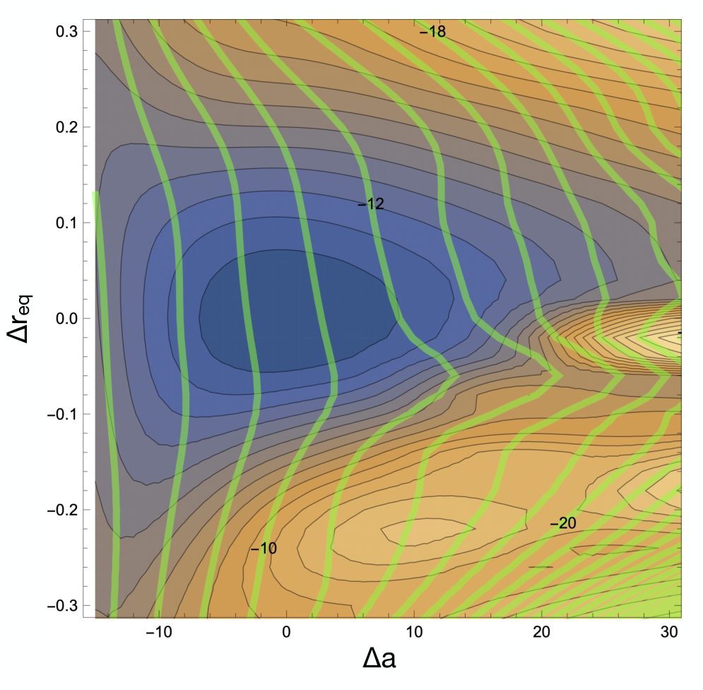
For a particular set of values of $a=20$ and $r_{eq}=1.5$ we computed the path ensemble. In figure 6, we show the $D_{KL}$, and the log rate constant $\ln k[a,r;\Delta a,\Delta r]$ on top of each other as a function of $\Delta a$ and $\Delta r$. As expected, the $D_{KL}$ is minimal for the reference value $\Delta a=0,\Delta r=0$, that is, at zero perturbation.

The reweighted rate constant is identical to the predicted rate constant from the prior path ensemble for $\Delta a=0,\Delta r=0$, but clearly varies if the system is perturbed. Note that $\Delta a$ seems to have the strongest effect in changing the rate. In contrast, for a similar change in $D_{KL}$ varying $\Delta r$ also changes the rate constant but not as dramatically. Indeed, the $D_{KL}$ is very sensitive to the $\Delta r$, already indicating that it is probably better to adjust $a$ than $r_{eq}$.

When we change the rate constant from the observed value of $\ln k_{AB}=-9$ to the new value $\ln k^{exp}$ we need to compute the derivatives and optimise the Lagrange function. We apply the method of Ref. Platt and Barr 1987. This iterative method starts at certain initial values and slowly converges to the solution. The solution for the most optimal set of $\{\Delta a,\Delta r\}$ is shown in table 2. In this table we show several sets of optimal solutions, as a function of imposed $k_{AB}^{exp}$. The first set shows the optimal solution for both $\Delta a$ and $\Delta r$. The other two sets we optimised for only one of the two parameters, and set the other to zero. From the value of $D_{KL}$ (which is identical to the negative of the Lagrange function $\mathcal{L}$ when the constraints are obeyed) it is clear that this is always less optimal than the two parameter solution, thus illustrating the need for multi-parameter force field optimization. Also note that the further the imposed $\ln k_{AB^{exp}}$ is from -9, the more $\mathcal{L}$, and thus $D_{KL}$ deviates.

References

- Brünger et al. (1998) A. T. Brünger, P. D. Adams, G. M. Clore, W. L. Delano, P. Gros, R. W. Grossekunstleve, J. S. Jiang, J. Kuszewski, M. Nilges, N. S. Pannu, R. J. Read, L. M. Rice, T. Simonson, and G. L. Warren, Acta Crystallogr. Sect. D Biol. Crystallogr. 54, 905 (1998).
- Bonomi et al. (2017) M. Bonomi, G. T. Heller, C. Camilloni, and M. Vendruscolo, Curr. Opin. Struct. Biol. 42, 106 (2017).
- Capelli et al. (2018) R. Capelli, G. Tiana, and C. Camilloni, J. Chem. Phys. 148, 184114 (2018).
- Brotzakis et al. (2021) Z. F. Brotzakis, M. Vendruscolo, and P. G. Bolhuis, Proceedings of the National Academy of Sciences 118, e2012423118 (2021).
- Alder and Wainwright (1957) B. J. Alder and T. E. Wainwright, J. Chem. Phys. 27, 1208 (1957).
- Frenkel and Smit (2001) D. Frenkel and B. Smit, Understanding Molecular Simulation, 2nd ed. (Academic Press, Inc., Orlando, FL, USA, 2001).
- Shaw et al. (2008) D. E. Shaw, M. M. Deneroff, R. O. Dror, J. S. Kuskin, R. H. Larson, J. K. Salmon, C. Young, B. Batson, K. J. Bowers, J. C. Chao, M. P. Eastwood, J. Gagliardo, and S. C. Gross, Commun. ACM 51, 91 (2008).
- Stone et al. (2007) J. E. Stone, J. C. Phillips, P. L. Freddolino, D. J. Hardy, L. G. Trabuco, and K. Schulten, J Comput Chem 28, 2618 (2007).
- Ciccotti et al. (2022) G. Ciccotti, C. Dellago, M. Ferrario, E. R. Hernández, and M. E. Tuckerman, European Physical Journal B 95 (2022), 10.1140/epjb/s10051-021-00249-x.
- Hollingsworth and Dror (2018) S. A. Hollingsworth and R. O. Dror, Neuron 99, 1129 (2018).
- Eyring (1935) H. Eyring, J. Chem. Phys. 3, 107 (1935).
- Chandler (1987) D. Chandler, Introduction to modern statistical mechanics (Oxford University Press, 1987).
- Bolhuis and Dellago (2010) P. G. Bolhuis and C. Dellago, Rev. Comput. Chem. 27, 1 (2010).
- Valsson et al. (2016) O. Valsson, P. Tiwary, and M. Parrinello, Annu. Rev. Phys. Chem. 67, 159 (2016).
- Harrison et al. (2018) J. A. Harrison, J. D. Schall, S. Maskey, P. T. Mikulski, M. T. Knippenberg, and B. H. Morrow, Applied Physics Reviews 5, 031104 (2018).
- Piana et al. (2011) S. Piana, K. Lindorff-Larsen, and D. E. Shaw, Biophysical journal 100, L47 (2011).
- van der Spoel (2021) D. van der Spoel, Current Opinion in Structural Biology 67, 18 (2021).
- Tkatchenko and Scheffler (2009) A. Tkatchenko and M. Scheffler, Phys. Rev. Lett. 102, 6 (2009).
- Zhang et al. (2018) L. Zhang, J. Han, H. Wang, R. Car, and E. Weinan, Phys. Rev. Let. 120, 143001 (2018), arXiv:1707.09571 .
- Bonati and Parrinello (2018) L. Bonati and M. Parrinello, Physical Review Letters 121, 265701 (2018), arXiv:1809.11088 .
- Singraber et al. (2019) A. Singraber, J. Behler, and C. Dellago, J. Chem. Theory Comput. 15, 1827 (2019).
- Lindorff-Larsen et al. (2012) K. Lindorff-Larsen, P. Maragakis, S. Piana, M. P. Eastwood, R. O. Dror, and D. E. Shaw, PloS one 7, e32131 (2012).
- Vitalini et al. (2015) F. Vitalini, A. S. Mey, F. Noé, and B. G. Keller, The Journal of Chemical Physics 142, 02B611_1 (2015).
- Cavalli et al. (2013) A. Cavalli, C. Camilloni, and M. Vendruscolo, J. Chem. Phys. 138, 094112 (2013).
- Boomsma et al. (2014) W. Boomsma, J. Ferkinghoff-Borg, and K. Lindorff-Larsen, PLoS Comput. Biol. 10, 1 (2014).
- Bonomi et al. (2015) M. Bonomi, C. Camilloni, A. Cavalli, and M. Vendruscolo, Sci. Adv. 2, 1 (2015).
- Bolhuis et al. (2021) P. G. Bolhuis, Z. F. Brotzakis, and M. Vendruscolo, The European Physical Journal B 94 (2021), 10.1140/epjb/s10051-021-00154-3.
- Tsai et al. (2022) S.-T. Tsai, E. Fields, and P. Tiwary, , 1 (2022), arXiv:2203.00597 .
- Cesari et al. (2019) A. Cesari, S. Bottaro, K. Lindorff-Larsen, P. Banáš, J. Šponer, and G. Bussi, Journal of Chemical Theory and Computation 15, 3425 (2019).
- Tesei et al. (2021) G. Tesei, T. K. Schulze, R. Crehuet, and K. Lindorff-Larsen, Proceedings of the National Academy of Sciences 118 (2021), 10.1073/pnas.2111696118.
- Fröhlking et al. (2020) T. Fröhlking, M. Bernetti, N. Calonaci, and G. Bussi, J. Chem. Phys. 152 (2020), 10.1063/5.0011346, arXiv:2004.01630 .
- Varela-Rial et al. (2022) A. Varela-Rial, I. Maryanow, M. Majewski, S. Doerr, N. Schapin, J. Jiménez-Luna, and G. De Fabritiis, Journal of Chemical Information and Modeling 62, 225 (2022).
- Qiu et al. (2021) Y. Qiu, D. G. A. Smith, S. Boothroyd, H. Jang, D. F. Hahn, J. Wagner, C. C. Bannan, T. Gokey, V. T. Lim, C. D. Stern, A. Rizzi, B. Tjanaka, G. Tresadern, X. Lucas, M. R. Shirts, M. K. Gilson, J. D. Chodera, C. I. Bayly, D. L. Mobley, and L.-P. Wang, J. Chem. Theory Comput. 17, 6262 (2021).
- Rose et al. (2021) D. C. Rose, J. F. Mair, and J. P. Garrahan, New Journal of Physics 23, 013013 (2021).
- Das et al. (2021) A. Das, D. C. Rose, J. P. Garrahan, and D. T. Limmer, The Journal of Chemical Physics 155, 134105 (2021).
- Das et al. (2022) A. Das, B. Kuznets-Speck, and D. T. Limmer, Phys. Rev. Lett. 128, 028005 (2022).
- Donati et al. (2017) L. Donati, C. Hartmann, and B. G. Keller, The Journal of chemical physics 146, 244112 (2017).
- Donati and Keller (2018) L. Donati and B. G. Keller, The Journal of chemical physics 149, 072335 (2018).
- Kieninger and Keller (2021) S. Kieninger and B. G. Keller, The Journal of Chemical Physics 154, 094102 (2021).
- Bolhuis et al. (2002) P. G. Bolhuis, D. Chandler, C. Dellago, and P. L. Geissler, Annu. Rev. Phys. Chem. 53, 291 (2002).
- Dellago et al. (2002) C. Dellago, P. Bolhuis, and P. Geissler, Advances in Chemical Physics 123 (2002).
- Du and Bolhuis (2013) W.-N. Du and P. G. Bolhuis, The Journal of Chemical Physics 139, 044105 (2013).
- Allen et al. (2005) R. J. Allen, P. B. Warren, and P. R. ten Wolde, Physical Review Letters 94 (2005), 10.1103/physrevlett.94.018104.
- Zuckerman and Chong (2017) D. M. Zuckerman and L. T. Chong, Annual Review of Biophysics 46, 43 (2017).
- Leimkuhler and Matthews (2015) B. Leimkuhler and C. Matthews, Interdisciplinary applied mathematics 36 (2015).
- Øksendal (2003) B. Øksendal, in Stochastic differential equations (Springer, 2003) pp. 65–84.
- Kloeden and Platen (1992) P. E. Kloeden and E. Platen, Numerical Solution of Stochastic Differential Equations., 1st ed. (Springer, Berlin, Heidelberg, 1992).
- Hazoglou et al. (2015) M. J. Hazoglou, V. Walther, P. D. Dixit, and K. A. Dill, The Journal of Chemical Physics 143, 051104 (2015).
- Chandler (1978) D. Chandler, J. Chem. Phys. 68, 2959 (1978).
- Faradjian and Elber (2004) A. K. Faradjian and R. Elber, Journal of Chemical Physics 120, 10880 (2004).
- Allen et al. (2006) R. J. Allen, D. Frenkel, and P. R. Ten Wolde, Journal of Chemical Physics 124 (2006), 10.1063/1.2140273, arXiv:0509499 [cond-mat] .
- Tiwary and Parrinello (2013) P. Tiwary and M. Parrinello, Physical Review Letters 111, 230602 (2013).
- Brotzakis and Bolhuis (2019) Z. F. Brotzakis and P. G. Bolhuis, Journal of Chemical Physics 151, 174111 (2019).
- van Erp et al. (2003) T. van Erp, D. Moroni, and P. Bolhuis, J of chem phys 118, 7762 (2003).
- Rogal et al. (2010) J. Rogal, W. Lechner, J. Juraszek, B. Ensing, and P. G. Bolhuis, J. Chem. Phys. 133, 174109 (2010).
- Dellago and Bolhuis (2004) C. Dellago and P. G. Bolhuis, Molecular Simulation 30, 795 (2004).
- Bolhuis and Csányi (2018) P. G. Bolhuis and G. Csányi, Physical Review Letters 120, 1 (2018).
- Ferrenberg, Alan M.; Swendsen, Robert (1989) H. Ferrenberg, Alan M.; Swendsen, Robert, Phys. Rev. Lett. 63, 1195 (1989), arXiv:0302123 [cond-mat] .
- Weeks et al. (1971) J. D. Weeks, D. Chandler, and H. C. Andersen, The Journal of Chemical Physics 54, 5237 (1971).
- Platt and Barr (1987) J. C. Platt and A. H. Barr, NIPS’87: Proceedings of the 1987 International Conference on Neural Information Processing Systems , 612–621 (1987).
- Copeland et al. (2006) R. A. Copeland, D. L. Pompliano, and T. D. Meek, Nat Rev Drug Discov 5, 730 (2006).
- Tonge (2018) P. J. Tonge, ACS Chemical Neuroscience 9, 29 (2018).
- Romano and Sciortino (2011) F. Romano and F. Sciortino, Nature Materials 10, 171 (2011).
- Oh et al. (2019) J. S. Oh, S. Lee, S. C. Glotzer, G. R. Yi, and D. J. Pine, Nature Communications 10 (2019), 10.1038/s41467-019-11915-1.
- Wang et al. (2019) Z. Wang, Z. Wang, J. Li, S. T. H. Cheung, C. Tian, S. H. Kim, G. R. Yi, E. Ducrot, and Y. Wang, Journal of the American Chemical Society 141, 14853 (2019).
- Zhang et al. (2020) S. Zhang, R. G. Alberstein, J. J. De Yoreo, and F. A. Tezcan, Nature Communications 11, 1 (2020).
- Fisher and Elbaum-Garfinkle (2020) R. S. Fisher and S. Elbaum-Garfinkle, Nature Communications 11 (2020), 10.1038/s41467-020-18224-y.
- Mitchell et al. (2021) M. J. Mitchell, M. M. Billingsley, R. M. Haley, M. E. Wechsler, N. A. Peppas, and R. Langer, Nature Reviews Drug Discovery 20, 101 (2021).
- Vijaykumar et al. (2016) A. Vijaykumar, P. G. Bolhuis, and P. R. ten Wolde, Faraday Discussions 195, 421 (2016).
- Vijaykumar et al. (2017) A. Vijaykumar, P. R. ten Wolde, and P. G. Bolhuis, The Journal of Chemical Physics 147, 184108 (2017).
- Winter et al. (2020) D. L. Winter, H. Iranmanesh, D. S. Clark, and D. J. Glover, ACS Synthetic Biology 9, 2132 (2020).
- Dignon et al. (2018) G. L. Dignon, W. Zheng, Y. C. Kim, R. B. Best, and J. Mittal, PLoS Computational Biology 14, 1 (2018).
- Best and Hummer (2016) R. B. Best and G. Hummer, Proceedings of the National Academy of Sciences of the United States of America 113, 3263 (2016).
- Senftle et al. (2016) T. P. Senftle, S. Hong, M. M. Islam, S. B. Kylasa, Y. Zheng, Y. K. Shin, C. Junkermeier, R. Engel-Herbert, M. J. Janik, H. M. Aktulga, T. Verstraelen, A. Grama, and A. C. Van Duin, npj Computational Materials 2 (2016), 10.1038/npjcompumats.2015.11.
- Rogal et al. (2019) J. Rogal, E. Schneider, and M. E. Tuckerman, Physical Review Letters 123, 245701 (2019), arXiv:1905.01536 .
- Bouchaud and Cont (1998) J.-p. Bouchaud and R. Cont, Eur. Phys. J. B. 6, 543 (1998), arXiv:9801279 [arXiv:cond-mat] .
- Haworth and Pope (1986) D. C. Haworth and S. B. Pope, Phys. Fluids 29, 387 (1986).
- Jones et al. (2020) L. D. Jones, M. Magdon-Ismail, L. Mersini-Houghton, and S. Meshnick, arXiv:2008.10530 , 1 (2020), arXiv:2008.10530 .