Neutrino Flavor Conversion, Advection, and Collisions: Towards the Full Solution
Abstract
At high densities in compact astrophysical sources, the coherent forward scattering of neutrinos onto each other is responsible for making the flavor evolution non-linear. Under the assumption of spherical symmetry, we present the first simulations tracking flavor transformation in the presence of neutrino-neutrino forward scattering, neutral and charged current collisions with the matter background, as well as neutrino advection. We find that, although flavor equipartition could be one of the solutions, it is not a generic outcome, as often postulated in the literature. Intriguingly, the strong interplay between flavor conversion, collisions, and advection leads to a spread of flavor conversion across the neutrino angular distributions and neighboring spatial regions. Our simulations show that slow and fast flavor transformation can occur simultaneously. In the light of this, looking for crossings in the electron neutrino lepton number as a diagnostic tool of the occurrence of flavor transformation in the high-density regime is a limiting method.
I Introduction
In neutrino-dense sources, such as core-collapse supernovae, the large number of neutrinos drives the source physics, despite the weakness of their interaction Burrows and Vartanyan 2021; Janka et al. 2016; Bethe and Wilson 1985; Colgate and White 1966; Wilson 1985. Tracking the neutrino flavor evolution in the source core is a complex task because, in addition to resonant conversion of neutrinos in matter Mikheyev and Smirnov 1985; Wolfenstein 1978, the coherent forward scattering of neutrinos on other neutrinos makes the flavor evolution non-linear Pantaleone 1992; Sigl and Raffelt 1993a; Duan et al. 2010; Mirizzi et al. 2016; Tamborra and Shalgar 2021. Neutrino self-interaction is a peculiar phenomenon: neutrinos with different momenta undergo flavor evolution with identical characteristic frequency Duan et al. 2007; Duan et al. 2006a; Duan et al. 2006b; Duan et al. 2006c; Fogli et al. 2007; Fogli et al. 2008; Raffelt and Smirnov 2007a; Hannestad et al. 2006.
In the context of core-collapse supernovae, collective neutrino oscillation was originally conceptualized within the “neutrino-bulb” model Duan et al. 2006b. The latter was based on the assumption of spherical symmetry and instantaneous decoupling of all neutrino flavors at a single radius. Within this framework, neutrino self-interaction leads to a swap in the energy distributions of the electron and non-electron flavors, the spectral split Duan et al. 2007; Duan et al. 2006b; Fogli et al. 2007; Fogli et al. 2008; Raffelt and Smirnov 2007a; Dasgupta et al. 2009; Fogli et al. 2009; Dasgupta et al. 2010; Friedland 2010. However, soon it was realized that the non-linear nature of neutrino collective effects leads to spontaneous breaking of symmetries Raffelt et al. 2013; Duan and Shalgar 2015.
Neutrinos of different flavors interact with matter differently. As a consequence, a crossing between the angular distributions of electron neutrinos and antineutrinos, the electron lepton number (ELN) crossing, may occur Shalgar and Tamborra 2019; Nagakura et al. 2021. Because of this feature, neutrinos experience a flavor instability, also in the limit of vanishing vacuum frequency Sawyer 2005; Sawyer 2009; Sawyer 2016; Chakraborty et al. 2016a; Chakraborty et al. 2016b; Tamborra and Shalgar 2021; Izaguirre et al. 2017; Yi et al. 2019; Martin et al. 2020. The flavor transformations resulting from such a flavor instability can occur at arbitrarily large neutrino number densities Sawyer 2005; Sawyer 2016; Tamborra and Shalgar 2021; Izaguirre et al. 2017; Shalgar and Tamborra 2021a; Shalgar et al. 2020; Shalgar and Tamborra 2021b; Johns et al. 2020a; Chakraborty and Chakraborty 2020; Abbar et al. 2019; Dasgupta et al. 2017. The corresponding characteristic frequency associated with flavor transformation can be very large, lending the phenomenon the name of “fast flavor conversion” to distinguish it from the ordinary neutrino self-interaction Chakraborty et al. 2016a; Tamborra and Shalgar 2021. The latter is also named “slow” collective oscillation since it is governed by a combination of the neutrino-neutrino self-interaction potential and the vacuum frequencies Duan et al. 2010; Mirizzi et al. 2016.
Despite being driven by the angular distributions of neutrinos, fast flavor conversion is further affected by the vacuum term and by the presence of all three neutrino flavors Shalgar and Tamborra 2021a; Chakraborty and Chakraborty 2020; Capozzi et al. 2020; Shalgar and Tamborra 2021b; Capozzi et al. 2022, as well as by symmetry breaking effects Shalgar and Tamborra 2022a. Moreover, collisions can enhance or suppress fast flavor transition according to the neutrino angular distributions Shalgar and Tamborra 2021c; Johns 2021; Hansen et al. 2022; Johns and Nagakura 2022; Martin et al. 2021; Shalgar and Tamborra 2022b. Unlike in the case of the neutrino-bulb model, which ignores the temporal dependence of the neutrino field due to advection, the motion of neutrinos can alter their momentum distribution; this can, in turn, affect the flavor evolution Shalgar et al. 2020; Richers et al. 2021a; Nagakura and Zaizen 2022; Shalgar and Tamborra 2022b.
Favorable conditions for the occurrence of fast flavor instabilities have been found in core-collapse supernovae as well as in compact binary merger remnants Xiong et al. 2020; Wu et al. 2017; Just et al. 2022; George et al. 2020; Li and Siegel 2021; Tamborra et al. 2017; Shalgar and Tamborra 2019; Abbar et al. 2019; Delfan Azari et al. 2019a; Delfan Azari et al. 2020; Delfan Azari et al. 2019b; Morinaga et al. 2020; Glas et al. 2020; Abbar et al. 2020; Nagakura et al. 2019; Abbar et al. 2021; Capozzi et al. 2021; Nagakura et al. 2021; Harada and Nagakura 2022. These developments have triggered intense research work aiming to assess the feedback of flavor transformation on the source physics. However, a deeper assessment of the extent of flavor conversion is still lacking.
This paper expands on our earlier work Shalgar and Tamborra 2022b, where we have reported on the impact of fast flavor conversion on the decoupling of neutrinos from matter in core-collapse supernovae. Our paper begins in Sec. II, where we introduce the formalism and outline the setup of our model. In Sec. III, we compute the classical steady state distribution of neutrinos in the absence of flavor transformation. First, we explore how the angular distributions of neutrinos evolve as functions of the radius and become forward peaked as neutrinos decouple from matter. Then, for illustrative purposes, we carry out the linear stability analysis restricting ourselves to the homogenous mode and by relying on the classical steady state distributions. Section IV focuses on the non-linear regime of flavor conversion in the presence of neutrino-neutrino interaction, advection, and collisions with the matter background. Finally, we discuss and summarize our findings in Sec. V. Appendix A provides additional details on the numerical convergence of the simulations.
II Problem setup
In this section, we introduce the neutrino equations of motion. Then, we provide details on the simulation setup and the parameters adopted to model the neutrino flavor evolution.
II.1 Neutrino equations of motion
For the sake of simplicity, we assume that neutrinos are monoenergetic and work in the two flavor approximation. However, note that additional modifications to the flavor conversion physics may be derived by relaxing such approximations Shalgar and Tamborra 2021b; Shalgar and Tamborra 2021a; Capozzi et al. 2022; Capozzi et al. 2020.
The evolution of flavor can be investigated in terms of Wigner transformed density matrices in the flavor space for neutrinos and antineutrinos, and , respectively. The diagonal elements of the density matrix, (with ), stand for the occupation numbers of neutrinos of different species, while the off-diagonal terms encode flavor coherence. As shown in Fig. 1, the parameter represents the radial direction, while is the angle with respect to the radial direction at the given , which should not be confused with the emission angle. The time variable is represented by .

The equations of motion that determine the flavor evolution of neutrinos and antineutrinos are given by Sigl and Raffelt 1993b:
| (1) | |||||
| (2) |
The left-hand sides of Eqs. 1 and 2 contain the total derivative, including the advective term. Due to the radial dependence of and the assumption of spherical symmetry, the advective term can be written as follows Rampp and Janka 2002:
| (3) | |||||
The right-hand sides of Eqs. 1 and 2 consist of the Hamiltonian that governs the flavor evolution and the collision term. The Hamiltonian includes the vacuum and self-interaction terms:
| (4) |
with
| (5) | |||
| (6) |
We use to denote the vacuum mixing angle, while is the vacuum frequency with being the neutrino energy. In the self-interaction Hamiltonian, , denotes the self-interaction strength. The additional integration over the azimuthal angle in Eq. 6 results in a factor , which has been absorbed in . Note that, due to the radial evolution of the angular distributions of neutrinos, the effective self-interaction strength decreases as a function of the radius in the regions beyond the neutrinosphere. The Hamiltonian governing the evolution of antineutrinos is the same as Eq. 4, with . The matter term in the Hamiltonian is neglected since its effect is to reduce the effective mixing angle of neutrinos Esteban-Pretel et al. 2008.
| (Cases A, B, C) | (Case A) | (Case B) | (Case C) | (Cases A, B, C) | |
|---|---|---|---|---|---|
| (km) | 1/[50 | 1/[50 | 1/[26 | 1/[30 | 1/[10 |
| (km) | 1/[50 | 1/[50 | 1/[25 | 1/[25 | 1/[10 |
| (km) | 1/[50 | 1/[25 | 1/[25 | 1/[25 | 1/[12.5 |
The collision term includes emission, absorption, and direction-changing collisions, respectively Weinberg 2019, i.e. it takes into account the main reactions of neutrinos with the matter background Shalgar and Tamborra 2019; Bowers and Wilson 1982; O’Connor 2015; Mezzacappa et al. 2020; Richers et al. 2019. This implies :
| (7) | |||||
| (8) | |||||
| (9) | |||||
Each of the above equations refers to all flavors as denoted by the superscripts. In principle, and the ratio among the different terms entering the collision term changes as a function of energy and time Bowers and Wilson 1982; O’Connor 2015; Mezzacappa et al. 2020; Richers et al. 2019. However, for the sake of simplicity, we omit any dependence on and . In addition, due to the small time scales associated with fast flavor evolution compared to the collision term, the off-diagonal components do not play any significant role (we have numerically verified that this assumption holds; results not shown here). We also neglect the Pauli blocking and neutrino chemical potentials for the sake of simplicity, although they should be taken into account once more a advanced modeling of the collision term is developed Bruenn 1985; Raffelt 1996.
II.2 Simulation setup
We carry out the simulations presented in this paper in a “simulation shell,” see gray shaded region in Fig 1. The radial range extends from km to km, while at each . We use a grid of uniform bins for both and . We have tested the convergence of the code with respect to the number of bins and provide further details in Appendix A. We use MeV eV2, km-1, and the effective vacuum mixing angle
At , the boundary condition is determined by the collision term. At , we impose two different boundary conditions depending on . For , neutrinos stream outward and, hence, the boundary condition is determined by conditions within the simulation region. For , we impose a vanishing boundary condition.
In order to investigate the dependence of fast flavor conversion on the shape of the ELN crossings, we consider three different collision terms: Cases A, B, and C, engineered to give different types of ELN crossings. Case A is also adopted in Ref. Shalgar and Tamborra 2022b. The flavor-dependent length-scales entering the collision terms in Eqs. 7–9 are reported in Table 1. For all collision terms, we use a simplified radial dependence defined by , with . We refer the reader to Appendix A of Ref. Shalgar and Tamborra 2022b for further details on the modeling of our heuristic collision term. We parametrize to have a characteristic length scale of – m at for all cases and so that falls exponentially as a function of . We stress that this is a simplification, not aiming to reproduce realistic conditions in the supernova core, but rather allowing to pass from isotropic to forward peaked distribution within the simulation shell and to generate an ELN crossing, as discussed in the next section. Since we populate the simulation shell through collisions, the collisions term for in Table 1 is chosen such that is within the trapping region and the neutrino number density there is governed only by the ratio of and .
The collision term involves factors that give rise to exponentially growing and damping solutions, which make them stiff. We use the Adams–Bashforth-Moulton method from the Differentialequations.jl package of Julia to solve the equations of motion Rackauckas and Nie 2017; Bezanson et al. 2017. Each simulation took CPU hours employing shared memory on the High Performance Computing Centre at the University of Copenhagen.
III Classical steady state configuration: no flavor conversion
In this section, we present our results on the classical steady state configuration achieved in the absence of flavor conversion. On the basis of these findings, we then introduce the linear stability analysis to investigate the regions in the simulation shell where the development of flavor instabilities is foreseen.
III.1 Angular distributions of neutrinos
In the absence of flavor conversion (i.e., in Eqs. 1 and 2), we aim to find a classical steady state configuration by setting as the initial condition for all flavors (the off-diagonal terms of the density matrices are initially equal to zero and remain as such throughout the evolution in the absence of flavor transformation) and by considering the collision and advection terms only.
Neutrinos in our setup are generated through collisions and advected across the simulation shell. The advective term allows for a change in the number density of neutrinos at a given location due to their motion. As for the collision term, the emission term is independent of the number density of neutrinos, the absorption term is proportional to the number density of neutrinos, while the direction changing term conserves the number of neutrinos. To obtain the steady state configuration, we need to evolve the neutrino field in our simulation shell at least for a period corresponding to the radial range , assuming that neutrinos travel at the speed of light, i.e. s. In the simulations, we have evolved the system for s out of caution.
The top panel of Fig. 2 shows a polar diagram of the angular distribution of for Case C, which we consider our benchmark configuration hereafter, once the steady state configuration is achieved. We obtain an isotropic configuration at small radii, which slowly becomes forward peaked at larger radii as the density falls. Such a trend holds for all flavors. However, as we move towards larger radii and the density falls, start forward peaking, followed by and , as displayed in the bottom panel of Fig. 2. This behavior can lead to ELN crossings and hence fast flavor instabilities. The qualitative trend in the angular distributions for Cases A and B is similar to the one of Case C and therefore not shown here.
The classical steady state obtained as described above constitutes the initial configuration adopted to solve the neutrino equations of motion including flavor conversion (see Sec. IV). This procedure is important from a numerical point of view. Any configuration that is not initially in a classical steady state leads to large gradients at the edges of the simulation shell, which give rise to numerical instabilities. Moreover, the advective term involves the calculation of the derivatives using a finite-element method, leading to numerical instabilities without sufficient resolution. Various tests have been carried out to make sure that numerical instabilities do not affect the results presented here.
III.2 Looking for flavor instabilities through the classical steady state solutions
It has been proven that the existence of ELN crossings is a necessary condition for fast flavor instabilities Morinaga 2022; Izaguirre et al. 2017. In order to gauge the presence of ELN crossings, we rely on a slightly modified definition of the parameter introduced in Ref. Padilla-Gay et al. 2021 and evaluate it at the time when the steady state configuration has been reached:
| (10) |
with
| (11) |
for and
| (12) |
for . The parameter can be different from zero if and only if there are regions in the angular domain where and other regions in the angular domain where , which implies the existence of an ELN crossing. Figure 3 shows the radial profile of for Cases A, B, and C. An ELN crossing exists for km for all cases; hence one should expect a potential flavor instability in this region.
To better gauge which regions of the simulation shell may be prone to flavor instabilities, we rely on the linear stability analysis of the classical steady state solution obtained in Sec. III.1 for Cases A, B, and C (see Tab. 1). In particular, we focus on flavor instabilities in the limit of vanishing and non-vanishing vacuum frequency (i.e., fast and slow flavor instabilities). For the sake of simplicity, we focus on the linear stability analysis for the homogeneous mode only, since we aim to gain insight on where flavor conversion may develop. This simplifying choice is also justified by the fact that if the neutrino gas is not homogeneous, as in our case, the equations for the Fourier modes are coupled. Note, however, that the numerical results presented in Sec. IV do not distinguish between homogeneous and inhomogeneous modes and do take into account collisions and advection.
To this purpose, we linearize Eqs. 1 and 2 ignoring the collision and advective terms. The linearization implies expanding the equations of motion for the off-diagonal components of the density matrix up to linear order in (and the same for ) Banerjee et al. 2011; Izaguirre et al. 2017. For each , the results are solutions for and of the form:
| (13) | |||
| (14) |
where is the eigenvalue which is independent of and it is the same for neutrinos and antineutrinos, due to the collective nature of the flavor evolution. The eigenvalue can be obtained semi-analytically and either is real or appears in complex-conjugate pairs. A complex with a non-zero imaginary part implies that and grow exponentially; this is known as flavor instability Banerjee et al. 2011.
The flavor instability thus obtained can be classified as a “fast” flavor instability, if it exists in the limit , and “slow” flavor instability otherwise. Note that this definition of slow flavor instability is a generalization of the one commonly adopted in the literature, invoking the existence of at least one crossing between the electron and non-electron flavors either in energy Raffelt and Smirnov 2007a; Raffelt and Smirnov 2007b; Fogli et al. 2008; Fogli et al. 2007; Dasgupta et al. 2009 or in angle Mirizzi and Serpico 2012a; Mirizzi and Serpico 2012b. The crossing would determine the development of a flavor instability while conserving the lepton number. As discussed later, the presence of ELN crossings (in angle) for our system of mono-energetic neutrinos is enough to guarantee the development of slow flavor instabilities for . The presence of a fast flavor instability requires that an ELN crossing occurs, which means that there is at least one angle for which . On the other hand, the presence of an ELN crossing does not necessarily imply the existence of a flavor instability or large flavor conversion Padilla-Gay et al. 2022; Padilla-Gay et al. 2021.
Figure 3 shows the growth rate of the flavor instability obtained by relying on the linear stability analysis. A non-zero value of the growth rate denotes the regions of flavor instability for and , and in the absence of advection and collisions. One can see that the parameter peaks in the same region where the flavor instability for is most prominent, confirming that the parameter is a good indicator of the regions of instability Padilla-Gay et al. 2021.
Figure 3 displays a substantial radial range where the flavor instability is present for all cases. However, not all regions that exhibit a flavor instability do so due to a fast flavor instability. In some radial regions, the flavor instability is due to slow collective modes, as can be seen by comparing the orange curve with the magenta one. Moreover, for Cases B and C, the growth rates for and coincide for some spatial regions. The growth rate for the fast flavor instability is much faster than the one of the slow flavor instability for the homogeneous mode, as seen by comparing the radial range for which only the slow flavor instability is present in Fig. 3 with the one where the fast instability occurs.
The fact that there are regions where the fast instabilities occur with the growth rate being strongly influenced by the vacuum term demands for a reassessment of the distinction between fast and slow flavor instabilities. In fact, the presence of a slow flavor instability near the decoupling region has not been shown in the literature before, because most studies do not follow the evolution of the angular distributions as functions of the radius or they just focus on one of the two instabilities ( or ). The implications of the presence of slow flavor instabilities near the decoupling region could show many more interesting results in multi-energy calculations because of the large vacuum frequency associated with the low energy tail of the neutrino distributions and its interplay with fast modes Shalgar and Tamborra 2021a; Duan et al. 2010; Mirizzi et al. 2016.
For both slow and fast instabilities, the absolute value of the eigenvectors determines the angular regions where flavor transformation first manifests itself for the homogeneous mode. Comparing the top and bottom panels of Fig. 4, we can see that the absolute value of the eigenvector for Case C peaks near the region of the ELN crossing (see also the bottom panel of Fig. 3 where the parameter peaks). It is also interesting to note that the absolute value of the eigenvector is zero or nearly zero in the proximity of (see Fig. 4). This divides the angular regions in two distinct regions which show qualitatively different flavor evolution, and flavor transformation in one domain () does not easily spread to the other domain (), as discussed in Sec. IV. From Fig. 3, we conclude that we should expect fast instabilities for and km, and slow instability for km. Interestingly, we can see from Fig. 4 that the slow instability for km still develops in the proximity of the ELN crossing, generalizing the findings of Refs. Mirizzi and Serpico 2012a; Mirizzi and Serpico 2012b.
IV Quasi steady state configuration: flavor conversion physics
In this section, we investigate the quasi steady state configuration reached by our system in the presence of flavor transformation. We then explore the effects of flavor conversion on neutrino decoupling, expanding on the findings of Ref. Shalgar and Tamborra 2022b, before to discuss the dynamical coupling among flavor conversion, collisions, and neutrino advection.
IV.1 Neutrino flavor transformation in the non-linear regime
In the presence of flavor conversion, this paper aims to find a “quasi steady state” solution of Eqs. 1 and 2. In fact, due to the non-linear nature of the flavor evolution, it is not possible to obtain a flavor configuration for which the neutrino flavor remains constant as a function of time for each and . The spatial and angular structures continue to evolve on smaller and smaller scales. The quasi steady state configuration should be reached by solving Eqs. 1 and 2 irrespective of the initial condition. However, from a numerical perspective, it is convenient to start with a configuration that is as close to the classical steady state configuration as possible.


Figure 5 shows a contour plot of the difference between with and without neutrino mixing in the plane spanned by and for Cases A, B, and C. The density matrix element, was calculated by using the classical steady state configuration () as the initial condition. The latter was then evolved up to s, which corresponds to the size of the simulation shell divided by the speed of light. If a smaller value of mixing angle is used, it takes longer for the system to reach the quasi steady state, but the results are unchanged.
By comparing with Figs. 5 and 3 and by taking into account the findings of Refs. Padilla-Gay et al. 2022; Shalgar and Tamborra 2022b, we conclude that looking for flavor instabilities is not enough to predict the radial regions actually affected by flavor conversion. In fact, the neutrinos that undergo flavor transformation at one radius are transported to larger radii due to advection. Cases B and C show an interesting phenomenology for the effect of advection and collisions, since the flavor instability is limited to a small range of the radial region (Fig. 3), but the actual region affected by flavor conversion is larger because of the dynamical effects induced by advection and collisions (Fig. 5).
The results from the numerical simulations show a spread in the flavor transformation to a finite domain of angular range, typically on one side of the ELN crossing as visible by comparing Figs. 3 and 6. To some extent, the essence of this phenomenon is captured in a homogeneous system with collisions Shalgar and Tamborra 2021c; Tamborra and Shalgar 2021.
From Fig. 6, we can also see that, as increases, the angular distributions become more forward peaked and the distributions of and are similar to each other. As a consequence, the angular distributions after flavor transformation of and tend to be similar to each other for certain , however, this does not imply that flavor equipartition is a general finding.
The spread of flavor transformed neutrinos from one radius to another is visible in the angle averaged neutrino occupation number as a function of the radius. We define the (quasi) steady state angle averaged neutrino number density as follows:
| (15) |
Figure 7 shows the radial profiles of for Cases A, B, and C. Note that in the absence of advection and collisions, unitary evolution dictates that lies in between and for all radii. However, due to the presence of advection and collision, Fig. 7 shows that this no longer holds; see for example Case B at km.
It is worth stressing that it is not possible to disentangle the effects of collisions and advection in our formalism. Nevertheless, their interplay ensures that neutrinos see different angular distributions over the simulation time, thus capturing the essence of the effects highlighted in Refs. Shalgar and Tamborra 2021c; Padilla-Gay et al. 2021.
IV.2 Effects of flavor transformation on neutrino decoupling
As discussed in Ref. Shalgar and Tamborra 2022b, the angle averaged number density of neutrinos of various flavors offers insight into the effect of flavor transformation on neutrino decoupling. In order to predict the region where decoupling approximately occurs, we consider the radius at which the flux factor for at the time when the quasi steady state configuration is reached,
| (16) |
We use this as an indicator of the effective decoupling radius since, in the coupled region, the neutrino angular distribution is isotropic, and the numerator vanishes. In the completely decoupled region, neutrinos are forward peaked and for all neutrinos; hence the flux factor is thus equal to unity.
Figure 7 shows the region where for Cases A, B, and C, generalizing the findings of Ref. Shalgar and Tamborra 2022b. However, as visible in some panels of Fig. 7, changes in the angle averaged neutrino occupation number are not always directly correlated to changes in the decoupling radius. This is a consequence of the non-trivial angular distributions arising from neutrino flavor transformation.
IV.3 Interplay among flavor transformation, collisions, and advection
The presence of collisions and advection redistributes neutrinos over the angle bins, as also found in Refs. Shalgar and Tamborra 2021c; Shalgar et al. 2020. In the absence of collisions and advection, flavor transformation is predominantly present in a narrow angular range around the ELN crossing. Moreover, in the regions where neutrino flavor transformation is present, the angular structure becomes progressively finer with time. Because of this, more angle bins are required as the simulation time increases, when Shalgar and Tamborra 2021a; Johns et al. 2020a; Johns et al. 2020b. However, the growth of structure at smaller and smaller scales is suppressed due to the presence of collisions and advection (see also Appendix A and Ref. Shalgar and Tamborra 2022b). This is not surprising and it is due to the fact that the collision term redistributes neutrinos across angles. More importantly, in the present case, neutrinos at different radii undergo flavor transformation at different angles at a given time. The advective term mixes the angular distribution at various radii as neutrinos travel, reducing the number of angular bins required to reach angular convergence.
The presence of flavor transformation in the angular range where and are approximately equal is a consequence of the assumption of azimuthal symmetry. In the absence of azimuthal symmetry, the flavor transformation is not necessarily correlated to the angular region in the proximity of the ELN crossing Shalgar and Tamborra 2022a.
Recent literature has speculated that flavor equipartition or depolarization may be a general outcome of fast flavor evolution Wu et al. 2021; Richers et al. 2021b; Bhattacharyya and Dasgupta 2021. Our findings suggest that this is not the case in our setup. Although we find equipartition in Case A, as shown in the top panel of Fig. 7, this is not true for Cases B and C. For Case A, flavor equipartition is reached because the occupation numbers of and are very similar in the classical steady state configuration. It is also important to note that this finding in our simulation setup is also linked to the fact that the lepton number in the neutrino sector is not conserved in our simulations due to absorption and emission collisional terms.
V Conclusions
Understanding the evolution of neutrino flavor in dense media remains an active subject of research. In this work, expanding on Ref. Shalgar and Tamborra 2022b, we investigate the flavor evolution for three different parametrizations of the collision term, consistently treating collision, advection, and flavor transformation. We rely on a spherically symmetric simulation shell and assume that all neutrinos have the same energy for simplicity. We populate the simulation shell through collisions and in the absence of flavor conversion, a steady state configuration is reached. In the presence of flavor transformation, flavor mixing spreads across angular and radial regions because of the dynamical effects induced by advection and collisions until a quasi steady state configuration is reached.
While in the literature flavor equipartition or depolarization is often presented as a general outcome of fast flavor conversion, we find that flavor equipartition is not achieved in general. Moreover, in the literature, it has been classically considered that fast flavor transformations could occur in the region of high density of neutrinos, while slow flavor collective transformations occur at larger radii and smaller densities; however, we find that an overlap between slow and fast flavor conversion could take place. This gives rise to a completely new phenomenology of neutrino self-interactions, yet to be explored.
Our work highlights the dynamical interplay among flavor conversion, advection, and collisions. In particular, we find that flavor conversion spreads across angular modes and in a larger spatial range, instead of remaining clustered in the proximity of the ELN crossing. On the other hand, the dynamical interplay among flavor conversion, advection, and collisions hinders the cascade of flavor structure to small scales, otherwise expected Shalgar and Tamborra 2021a; Johns et al. 2020a; Johns et al. 2020b, and smears the quasi steady state distributions.
Because of the numerical challenges, our model includes some simplifications. The ones which further need to be relaxed concern the dependence on energy of flavor transformation and the collision term. In fact, fast flavor conversion is by itself not sensitive to neutrino energy, but slow flavor conversion is. Hence, a non-trivial interplay between collisions and slow flavor conversion may exist.
This work highlights the fascinating nature of neutrino self-interaction in compact astrophysical sources and the non-trivial interplay of the flavor conversion physics with neutrino advection and collisions. As such, our findings give a glimpse of flavor phenomenology that could have potentially interesting implications for the physics of compact sources and remains to be explored.
Acknowledgements.
We would like to thank Rasmus S.L. Hansen and Christopher Rackauckas for insightful discussions. We acknowledge support from the Villum Foundation (Project No. 13164), the Danmarks Frie Forskningsfonds (Project No. 8049-00038B), the MERAC Foundation, and the Deutsche Forschungsgemeinschaft through Sonderforschungbereich SFB 1258 “Neutrinos and Dark Matter in Astro- and Particle Physics” (NDM).Appendix A Numerical convergence
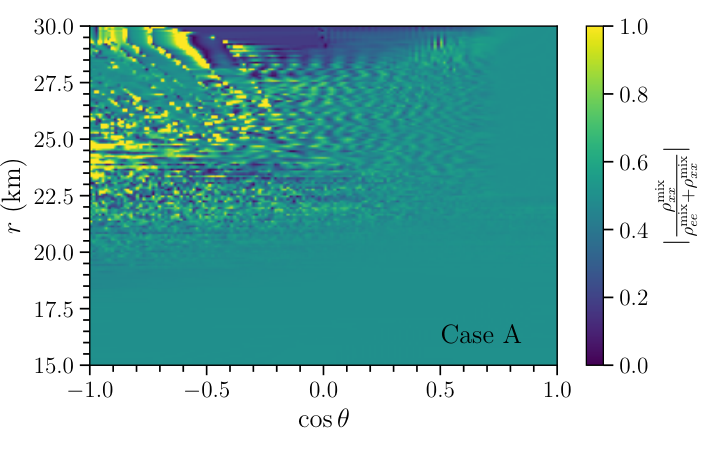
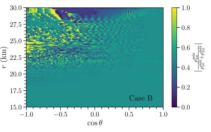
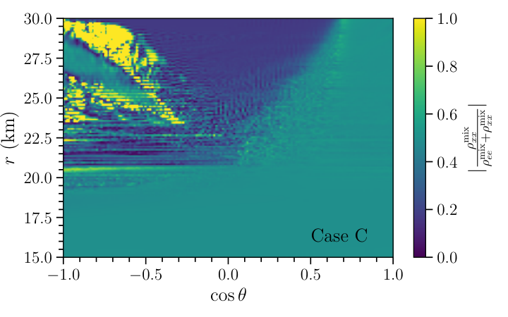
To prove numerical convergence, Fig. 8 shows the analogous of Fig. 5, but with simulations obtained by using bins, while keeping all other inputs unchanged. One can see that the agreement between the two figures is excellent.


Naively, one might expect that the simulation radial resolution should be dictated by (as it would be the case in the absence of advection, collisions, and the vacuum term). However this is not the case in our simulation setup, because of the inclusion of neutrino advection and collisions. To this purpose, we consider two simulation sets, one with km-1 and the other one with km-1, and for each , we run two simulations, one with and one with radial bins for Case A, while all other inputs are kept unchanged. Figure 9 shows the results: while minor differences are appreciable, the overall trend is robust. The cascade of the large scale inhomogeneous modes to small scales occurs at a rate that advection and collisions are not able to erase only for km-1. For km-1 and 1500 radial bins, we resolve resolve spatial scales of order and show that our conclusions are not affected.
To quantify the differences between the cases with different resolution in Fig. 9, we compute the relative error by coarse-graining the results with radial bins and averaging over batches of radial bins to compare the results with the ones from the numerical simulation with radial bins. At each radius, the error is defined as relative error between the angle averaged population densities. We further average the relative error over all the radial bins to calculate the average relative error (see Ref. Shalgar and Tamborra 2022b for additional details). The average relative error at s between the two simulations with different number of radial bins is for km-1 and for km-1. The figures demonstrate that the eventual existence of structures at small length scales of size does not affect the results qualitatively even if the spatial resolution is not of that order. These findings are also in agreement with the ones presented in Refs. Shalgar et al. 2020; Padilla-Gay et al. 2021; Shalgar and Tamborra 2021c. Figure 10 shows for Cases A, B, and C using the default value of km-1 for the sake of completeness. In addition, Fig. 11 shows the same quantity for lower value of for Case A (see also Fig. 9). Note that some of these plots should be interpreted with caution because of numerical artifacts in the top-left region where the denominator is very small.




References
- Burrows and Vartanyan (2021) Adam Burrows and David Vartanyan, “Core-Collapse Supernova Explosion Theory,” Nature 589, 29–39 (2021), arXiv:2009.14157 [astro-ph.SR] .
- Janka et al. (2016) Hans-Thomas Janka, Tobias Melson, and Alexander Summa, “Physics of Core-Collapse Supernovae in Three Dimensions: a Sneak Preview,” Ann. Rev. Nucl. Part. Sci. 66, 341–375 (2016), arXiv:1602.05576 [astro-ph.SR] .
- Bethe and Wilson (1985) Hans A. Bethe and James R. Wilson, “Revival of a stalled supernova shock by neutrino heating,” Astrophys. J. 295, 14–23 (1985).
- Colgate and White (1966) Stirling A. Colgate and Richard H. White, “The Hydrodynamic Behavior of Supernovae Explosions,” Astrophys. J. 143, 626 (1966).
- Wilson (1985) James R. Wilson, “Supernovae and Post-Collapse Behavior,” in Numerical Astrophysics (1985) p. 422.
- Mikheyev and Smirnov (1985) Stanislav P. Mikheyev and Alexei Yu. Smirnov, “Resonance enhancement of oscillations in matter and solar neutrino spectroscopy,” Yadernaya Fizika 42, 1441–1448 (1985).
- Wolfenstein (1978) Lincoln Wolfenstein, “Neutrino oscillations in matter,” Phys. Rev. D 17, 2369–2374 (1978).
- Pantaleone (1992) James T. Pantaleone, “Neutrino oscillations at high densities,” Phys. Lett. B 287, 128–132 (1992).
- Sigl and Raffelt (1993a) Günther Sigl and Georg G. Raffelt, “General kinetic description of relativistic mixed neutrinos,” Nucl. Phys. B 406, 423–451 (1993a).
- Duan et al. (2010) Huaiyu Duan, George M. Fuller, and Yong-Zhong Qian, “Collective Neutrino Oscillations,” Ann. Rev. Nucl. Part. Sci. 60, 569–594 (2010), arXiv:1001.2799 [hep-ph] .
- Mirizzi et al. (2016) Alessandro Mirizzi, Irene Tamborra, Hans-Thomas Janka, Ninetta Saviano, Kate Scholberg, Robert Bollig, Lorenz Hüdepohl, and Sovan Chakraborty, “Supernova Neutrinos: Production, Oscillations and Detection,” Riv. Nuovo Cim. 39, 1–112 (2016), arXiv:1508.00785 [astro-ph.HE] .
- Tamborra and Shalgar (2021) Irene Tamborra and Shashank Shalgar, “New Developments in Flavor Evolution of a Dense Neutrino Gas,” Ann. Rev. Nucl. Part. Sci. 71, 165–188 (2021), arXiv:2011.01948 [astro-ph.HE] .
- Duan et al. (2007) Huaiyu Duan, George M. Fuller, J. Carlson, and Yong-Zhong Qian, “Neutrino Mass Hierarchy and Stepwise Spectral Swapping of Supernova Neutrino Flavors,” Phys. Rev. Lett. 99, 241802 (2007), arXiv:0707.0290 [astro-ph] .
- Duan et al. (2006a) Huaiyu Duan, George M. Fuller, J. Carlson, and Yong-Zhong Qian, “Coherent Development of Neutrino Flavor in the Supernova Environment,” Phys. Rev. Lett. 97, 241101 (2006a), arXiv:astro-ph/0608050 [astro-ph] .
- Duan et al. (2006b) Huaiyu Duan, George M. Fuller, J Carlson, and Yong-Zhong Qian, “Simulation of Coherent Non-Linear Neutrino Flavor Transformation in the Supernova Environment. 1. Correlated Neutrino Trajectories,” Phys. Rev. D74, 105014 (2006b), arXiv:astro-ph/0606616 [astro-ph] .
- Duan et al. (2006c) Huaiyu Duan, George M. Fuller, and Yong-Zhong Qian, “Collective neutrino flavor transformation in supernovae,” Phys. Rev. D 74, 123004 (2006c), arXiv:astro-ph/0511275 [astro-ph] .
- Fogli et al. (2007) Gianluigi Fogli, Eligio Lisi, Antonio Marrone, and Alessandro Mirizzi, “Collective neutrino flavor transitions in supernovae and the role of trajectory averaging,” JCAP 12, 010 (2007), arXiv:0707.1998 [hep-ph] .
- Fogli et al. (2008) Gianluigi Fogli, Eligio Lisi, Antonio Marrone, Alessandro Mirizzi, and Irene Tamborra, “Low-energy spectral features of supernova (anti)neutrinos in inverted hierarchy,” Phys. Rev. D 78, 097301 (2008), arXiv:0808.0807 [hep-ph] .
- Raffelt and Smirnov (2007a) Georg G. Raffelt and Alexei Yu. Smirnov, “Self-induced spectral splits in supernova neutrino fluxes,” Phys. Rev. D 76, 081301 (2007a), [Erratum: Phys.Rev.D 77, 029903 (2008)], arXiv:0705.1830 [hep-ph] .
- Hannestad et al. (2006) Steen Hannestad, Georg G. Raffelt, Gunter Sigl, and Yvonne Y. Y. Wong, “Self-induced conversion in dense neutrino gases: Pendulum in flavour space,” Phys. Rev. D 74, 105010 (2006), [Erratum: Phys.Rev.D 76, 029901 (2007)], arXiv:astro-ph/0608695 .
- Dasgupta et al. (2009) Basudeb Dasgupta, Amol Dighe, Georg G. Raffelt, and Alexei Yu. Smirnov, “Multiple Spectral Splits of Supernova Neutrinos,” Phys. Rev. Lett. 103, 051105 (2009), arXiv:0904.3542 [hep-ph] .
- Fogli et al. (2009) Gianluigi Fogli, Eligio Lisi, Antonio Marrone, and Irene Tamborra, “Supernova neutrinos and antineutrinos: Ternary luminosity diagram and spectral split patterns,” JCAP 10, 002 (2009), arXiv:0907.5115 [hep-ph] .
- Dasgupta et al. (2010) Basudeb Dasgupta, Alessandro Mirizzi, Irene Tamborra, and Ricard Tomas, “Neutrino mass hierarchy and three-flavor spectral splits of supernova neutrinos,” Phys. Rev. D 81, 093008 (2010), arXiv:1002.2943 [hep-ph] .
- Friedland (2010) Alexander Friedland, “Self-refraction of supernova neutrinos: mixed spectra and three-flavor instabilities,” Phys. Rev. Lett. 104, 191102 (2010), arXiv:1001.0996 [hep-ph] .
- Raffelt et al. (2013) Georg G. Raffelt, Srdjan Sarikas, and David de Sousa Seixas, “Axial Symmetry Breaking in Self-Induced Flavor Conversion of Supernova Neutrino Fluxes,” Phys. Rev. Lett. 111, 091101 (2013), [Erratum: Phys. Rev. Lett.113,no.23,239903(2014)], arXiv:1305.7140 [hep-ph] .
- Duan and Shalgar (2015) Huaiyu Duan and Shashank Shalgar, “Flavor instabilities in the neutrino line model,” Phys. Lett. B747, 139–143 (2015), arXiv:1412.7097 [hep-ph] .
- Shalgar and Tamborra (2019) Shashank Shalgar and Irene Tamborra, “On the Occurrence of Crossings Between the Angular Distributions of Electron Neutrinos and Antineutrinos in the Supernova Core,” Astrophys. J. 883, 80 (2019), arXiv:1904.07236 [astro-ph.HE] .
- Nagakura et al. (2021) Hiroki Nagakura, Lucas Johns, Adam Burrows, and George M. Fuller, “Where, when, and why: Occurrence of fast-pairwise collective neutrino oscillation in three-dimensional core-collapse supernova models,” Phys. Rev. D 104, 083025 (2021), arXiv:2108.07281 [astro-ph.HE] .
- Sawyer (2005) Raymond F. Sawyer, “Speed-up of neutrino transformations in a supernova environment,” Phys. Rev. D 72, 045003 (2005), arXiv:hep-ph/0503013 .
- Sawyer (2009) Raymond F. Sawyer, “The multi-angle instability in dense neutrino systems,” Phys. Rev. D 79, 105003 (2009), arXiv:0803.4319 [astro-ph] .
- Sawyer (2016) Raymond F. Sawyer, “Neutrino cloud instabilities just above the neutrino sphere of a supernova,” Phys. Rev. Lett. 116, 081101 (2016), arXiv:1509.03323 [astro-ph.HE] .
- Chakraborty et al. (2016a) Sovan Chakraborty, Rasmus Hansen, Ignacio Izaguirre, and Georg G. Raffelt, “Collective neutrino flavor conversion: Recent developments,” Nucl. Phys. B 908, 366–381 (2016a), arXiv:1602.02766 [hep-ph] .
- Chakraborty et al. (2016b) Sovan Chakraborty, Rasmus Sloth Hansen, Ignacio Izaguirre, and Georg G. Raffelt, “Self-induced neutrino flavor conversion without flavor mixing,” JCAP 03, 042 (2016b), arXiv:1602.00698 [hep-ph] .
- Izaguirre et al. (2017) Ignacio Izaguirre, Georg G. Raffelt, and Irene Tamborra, “Fast Pairwise Conversion of Supernova Neutrinos: A Dispersion-Relation Approach,” Phys. Rev. Lett. 118, 021101 (2017), arXiv:1610.01612 [hep-ph] .
- Yi et al. (2019) Changhao Yi, Lei Ma, Joshua D. Martin, and Huaiyu Duan, “Dispersion relation of the fast neutrino oscillation wave,” Phys. Rev. D 99, 063005 (2019), arXiv:1901.01546 [hep-ph] .
- Martin et al. (2020) Joshua D. Martin, Changhao Yi, and Huaiyu Duan, “Dynamic fast flavor oscillation waves in dense neutrino gases,” Phys. Lett. B 800, 135088 (2020), arXiv:1909.05225 [hep-ph] .
- Shalgar and Tamborra (2021a) Shashank Shalgar and Irene Tamborra, “Dispelling a myth on dense neutrino media: fast pairwise conversions depend on energy,” JCAP 01, 014 (2021a), arXiv:2007.07926 [astro-ph.HE] .
- Shalgar et al. (2020) Shashank Shalgar, Ian Padilla-Gay, and Irene Tamborra, “Neutrino propagation hinders fast pairwise flavor conversions,” JCAP 06, 048 (2020), arXiv:1911.09110 [astro-ph.HE] .
- Shalgar and Tamborra (2021b) Shashank Shalgar and Irene Tamborra, “Three flavor revolution in fast pairwise neutrino conversion,” Phys. Rev. D 104, 023011 (2021b), arXiv:2103.12743 [hep-ph] .
- Johns et al. (2020a) Lucas Johns, Hiroki Nagakura, George M. Fuller, and Adam Burrows, “Neutrino oscillations in supernovae: angular moments and fast instabilities,” Phys. Rev. D 101, 043009 (2020a), arXiv:1910.05682 [hep-ph] .
- Chakraborty and Chakraborty (2020) Madhurima Chakraborty and Sovan Chakraborty, “Three flavor neutrino conversions in supernovae: slow & fast instabilities,” JCAP 01, 005 (2020), arXiv:1909.10420 [hep-ph] .
- Abbar et al. (2019) Sajad Abbar, Huaiyu Duan, Kohsuke Sumiyoshi, Tomoya Takiwaki, and Maria Cristina Volpe, “On the occurrence of fast neutrino flavor conversions in multidimensional supernova models,” Phys. Rev. D100, 043004 (2019), arXiv:1812.06883 [astro-ph.HE] .
- Dasgupta et al. (2017) Basudeb Dasgupta, Alessandro Mirizzi, and Manibrata Sen, “Fast neutrino flavor conversions near the supernova core with realistic flavor-dependent angular distributions,” JCAP 02, 019 (2017), arXiv:1609.00528 [hep-ph] .
- Capozzi et al. (2020) Francesco Capozzi, Madhurima Chakraborty, Sovan Chakraborty, and Manibrata Sen, “Fast flavor conversions in supernovae: the rise of mu-tau neutrinos,” Phys. Rev. Lett. 125, 251801 (2020), arXiv:2005.14204 [hep-ph] .
- Capozzi et al. (2022) Francesco Capozzi, Madhurima Chakraborty, Sovan Chakraborty, and Manibrata Sen, “Supernova fast flavor conversions in 1+1D: Influence of mu-tau neutrinos,” Phys. Rev. D 106, 083011 (2022), arXiv:2205.06272 [hep-ph] .
- Shalgar and Tamborra (2022a) Shashank Shalgar and Irene Tamborra, “Symmetry breaking induced by pairwise conversion of neutrinos in compact sources,” Phys. Rev. D 105, 043018 (2022a), arXiv:2106.15622 [hep-ph] .
- Shalgar and Tamborra (2021c) Shashank Shalgar and Irene Tamborra, “A change of direction in pairwise neutrino conversion physics: The effect of collisions,” Phys. Rev. D 103, 063002 (2021c), arXiv:2011.00004 [astro-ph.HE] .
- Johns (2021) Lucas Johns, “Collisional flavor instabilities of supernova neutrinos,” (2021), arXiv:2104.11369 [hep-ph] .
- Hansen et al. (2022) Rasmus S. L. Hansen, Shashank Shalgar, and Irene Tamborra, “Enhancement or damping of fast neutrino flavor conversions due to collisions,” Phys. Rev. D 105, 123003 (2022), arXiv:2204.11873 [astro-ph.HE] .
- Johns and Nagakura (2022) Lucas Johns and Hiroki Nagakura, “Self-consistency in models of neutrino scattering and fast flavor conversion,” Phys. Rev. D 106, 043031 (2022), arXiv:2206.09225 [hep-ph] .
- Martin et al. (2021) Joshua D. Martin, J. Carlson, Vincenzo Cirigliano, and Huaiyu Duan, “Fast flavor oscillations in dense neutrino media with collisions,” Phys. Rev. D 103, 063001 (2021), arXiv:2101.01278 [hep-ph] .
- Shalgar and Tamborra (2022b) Shashank Shalgar and Irene Tamborra, “Supernova Neutrino Decoupling Is Altered by Flavor Conversion,” (2022b), arXiv:2206.00676 [hep-ph] .
- Richers et al. (2021a) Sherwood Richers, Donald Willcox, and Nicole Ford, “Neutrino fast flavor instability in three dimensions,” Phys. Rev. D 104, 103023 (2021a), arXiv:2109.08631 [astro-ph.HE] .
- Nagakura and Zaizen (2022) Hiroki Nagakura and Masamichi Zaizen, “Time-Dependent and Quasisteady Features of Fast Neutrino-Flavor Conversion,” Phys. Rev. Lett. 129, 261101 (2022), arXiv:2206.04097 [astro-ph.HE] .
- Xiong et al. (2020) Zewei Xiong, Andre Sieverding, Manibrata Sen, and Yong-Zhong Qian, “Potential Impact of Fast Flavor Oscillations on Neutrino-driven Winds and Their Nucleosynthesis,” Astrophys. J. 900, 144 (2020), arXiv:2006.11414 [astro-ph.HE] .
- Wu et al. (2017) Meng-Ru Wu, Irene Tamborra, Oliver Just, and Hans-Thomas Janka, “Imprints of neutrino-pair flavor conversions on nucleosynthesis in ejecta from neutron-star merger remnants,” Phys. Rev. D 96, 123015 (2017), arXiv:1711.00477 [astro-ph.HE] .
- Just et al. (2022) Oliver Just, Sajad Abbar, Meng-Ru Wu, Irene Tamborra, Hans-Thomas Janka, and Francesco Capozzi, “Fast neutrino conversion in hydrodynamic simulations of neutrino-cooled accretion disks,” Phys. Rev. D 105, 083024 (2022), arXiv:2203.16559 [astro-ph.HE] .
- George et al. (2020) Manu George, Meng-Ru Wu, Irene Tamborra, Ricard Ardevol-Pulpillo, and Hans-Thomas Janka, “Fast neutrino flavor conversion, ejecta properties, and nucleosynthesis in newly-formed hypermassive remnants of neutron-star mergers,” Phys. Rev. D 102, 103015 (2020), arXiv:2009.04046 [astro-ph.HE] .
- Li and Siegel (2021) Xinyu Li and Daniel M. Siegel, “Neutrino Fast Flavor Conversions in Neutron-Star Postmerger Accretion Disks,” Phys. Rev. Lett. 126, 251101 (2021), arXiv:2103.02616 [astro-ph.HE] .
- Tamborra et al. (2017) Irene Tamborra, Lorenz Hüdepohl, Georg G. Raffelt, and Hans-Thomas Janka, “Flavor-dependent neutrino angular distribution in core-collapse supernovae,” Astrophys. J. 839, 132 (2017), arXiv:1702.00060 [astro-ph.HE] .
- Delfan Azari et al. (2019a) Milad Delfan Azari, Shoichi Yamada, Taiki Morinaga, Wakana Iwakami, Hirotada Okawa, Hiroki Nagakura, and Kohsuke Sumiyoshi, “Linear Analysis of Fast-Pairwise Collective Neutrino Oscillations in Core-Collapse Supernovae based on the Results of Boltzmann Simulations,” Phys. Rev. D99, 103011 (2019a), arXiv:1902.07467 [astro-ph.HE] .
- Delfan Azari et al. (2020) Milad Delfan Azari, Shoichi Yamada, Taiki Morinaga, Hiroki Nagakura, Shun Furusawa, Akira Harada, Hirotada Okawa, Wakana Iwakami, and Kohsuke Sumiyoshi, “Fast collective neutrino oscillations inside the neutrino sphere in core-collapse supernovae,” Phys. Rev. D 101, 023018 (2020), arXiv:1910.06176 [astro-ph.HE] .
- Delfan Azari et al. (2019b) Milad Delfan Azari, Shoichi Yamada, Taiki Morinaga, Wakana Iwakami, Hirotada Okawa, Hiroki Nagakura, and Kohsuke Sumiyoshi, “Linear Analysis of Fast-Pairwise Collective Neutrino Oscillations in Core-Collapse Supernovae based on the Results of Boltzmann Simulations,” Phys. Rev. D 99, 103011 (2019b), arXiv:1902.07467 [astro-ph.HE] .
- Morinaga et al. (2020) Taiki Morinaga, Hiroki Nagakura, Chinami Kato, and Shoichi Yamada, “Fast neutrino-flavor conversion in the preshock region of core-collapse supernovae,” Physical Review Research 2, 012046 (2020), arXiv:1909.13131 [astro-ph.HE] .
- Glas et al. (2020) Robert Glas, Hans-Thomas Janka, Francesco Capozzi, Manibrata Sen, Basudeb Dasgupta, Alessandro Mirizzi, and Guenter Sigl, “Fast Neutrino Flavor Instability in the Neutron-star Convection Layer of Three-dimensional Supernova Models,” Phys. Rev. D 101, 063001 (2020), arXiv:1912.00274 [astro-ph.HE] .
- Abbar et al. (2020) Sajad Abbar, Huaiyu Duan, Kohsuke Sumiyoshi, Tomoya Takiwaki, and Maria Cristina Volpe, “Fast Neutrino Flavor Conversion Modes in Multidimensional Core-collapse Supernova Models: the Role of the Asymmetric Neutrino Distributions,” Phys. Rev. D 101, 043016 (2020), arXiv:1911.01983 [astro-ph.HE] .
- Nagakura et al. (2019) Hiroki Nagakura, Taiki Morinaga, Chinami Kato, and Shoichi Yamada, “Fast-pairwise Collective Neutrino Oscillations Associated with Asymmetric Neutrino Emissions in Core-collapse Supernovae,” Astrophys. J. 886, 139 (2019), arXiv:1910.04288 [astro-ph.HE] .
- Abbar et al. (2021) Sajad Abbar, Francesco Capozzi, Robert Glas, H. Thomas Janka, and Irene Tamborra, “On the characteristics of fast neutrino flavor instabilities in three-dimensional core-collapse supernova models,” Phys. Rev. D 103, 063033 (2021), arXiv:2012.06594 [astro-ph.HE] .
- Capozzi et al. (2021) Francesco Capozzi, Sajad Abbar, Robert Bollig, and Hans-Thomas Janka, “Fast neutrino flavor conversions in one-dimensional core-collapse supernova models with and without muon creation,” Phys. Rev. D 103, 063013 (2021), arXiv:2012.08525 [astro-ph.HE] .
- Harada and Nagakura (2022) Akira Harada and Hiroki Nagakura, “Prospects of Fast Flavor Neutrino Conversion in Rotating Core-collapse Supernovae,” Astrophys. J. 924, 109 (2022), arXiv:2110.08291 [astro-ph.HE] .
- Sigl and Raffelt (1993b) G. Sigl and G. G. Raffelt, “General kinetic description of relativistic mixed neutrinos,” Nucl. Phys. B 406, 423–451 (1993b).
- Rampp and Janka (2002) Markus Rampp and H. Thomas Janka, “Radiation hydrodynamics with neutrinos: Variable Eddington factor method for core collapse supernova simulations,” Astron. Astrophys. 396, 361 (2002), arXiv:astro-ph/0203101 .
- Esteban-Pretel et al. (2008) A. Esteban-Pretel, A. Mirizzi, S. Pastor, R. Tomas, G. G. Raffelt, P. D. Serpico, and G. Sigl, “Role of dense matter in collective supernova neutrino transformations,” Phys. Rev. D 78, 085012 (2008), arXiv:0807.0659 [astro-ph] .
- Weinberg (2019) Steven Weinberg, Lectures on Astrophysics (Cambridge University Press, 2019).
- Bowers and Wilson (1982) R. L. Bowers and J. R. Wilson, “A numerical model for stellar core collapse calculations.” Astrophys. J. Suppl. 50, 115–159 (1982).
- O’Connor (2015) Evan O’Connor, “An Open-Source Neutrino Radiation Hydrodynamics Code for Core-Collapse Supernovae,” Astrophys. J. Suppl. 219, 24 (2015), arXiv:1411.7058 [astro-ph.HE] .
- Mezzacappa et al. (2020) Anthony Mezzacappa, Eirik Endeve, O. E. Bronson Messer, and Stephen W. Bruenn, “Physical, numerical, and computational challenges of modeling neutrino transport in core-collapse supernovae,” Liv. Rev. Comput. Astrophys. 6, 4 (2020), arXiv:2010.09013 [astro-ph.HE] .
- Richers et al. (2019) Sherwood A. Richers, Gail C. McLaughlin, James P. Kneller, and Alexey Vlasenko, “Neutrino Quantum Kinetics in Compact Objects,” Phys. Rev. D 99, 123014 (2019), arXiv:1903.00022 [astro-ph.HE] .
- Bruenn (1985) S. W. Bruenn, “Stellar core collapse - Numerical model and infall epoch,” Astrophys. J. Suppl. 58, 771–841 (1985).
- Raffelt (1996) G. G. Raffelt, Stars as laboratories for fundamental physics: The astrophysics of neutrinos, axions, and other weakly interacting particles (1996).
- Rackauckas and Nie (2017) Christopher Rackauckas and Qing Nie, “Differentialequations.jl–a performant and feature-rich ecosystem for solving differential equations in julia,” Journal of Open Research Software 5 (2017).
- Bezanson et al. (2017) Jeff Bezanson, Alan Edelman, Stefan Karpinski, and Viral B Shah, “Julia: A fresh approach to numerical computing,” SIAM Review 59, 65–98 (2017).
- Morinaga (2022) Taiki Morinaga, “Fast neutrino flavor instability and neutrino flavor lepton number crossings,” Phys. Rev. D 105, L101301 (2022), arXiv:2103.15267 [hep-ph] .
- Padilla-Gay et al. (2021) Ian Padilla-Gay, Shashank Shalgar, and Irene Tamborra, “Multi-Dimensional Solution of Fast Neutrino Conversions in Binary Neutron Star Merger Remnants,” JCAP 01, 017 (2021), arXiv:2009.01843 [astro-ph.HE] .
- Banerjee et al. (2011) Arka Banerjee, Amol Dighe, and Georg G. Raffelt, “Linearized flavor-stability analysis of dense neutrino streams,” Phys. Rev. D 84, 053013 (2011), arXiv:1107.2308 [hep-ph] .
- Raffelt and Smirnov (2007b) Georg G. Raffelt and Alexei Yu. Smirnov, “Adiabaticity and spectral splits in collective neutrino transformations,” Phys. Rev. D 76, 125008 (2007b), arXiv:0709.4641 [hep-ph] .
- Mirizzi and Serpico (2012a) Alessandro Mirizzi and Pasquale D. Serpico, “Instability in the Dense Supernova Neutrino Gas with Flavor-Dependent Angular Distributions,” Phys. Rev. Lett. 108, 231102 (2012a), arXiv:1110.0022 [hep-ph] .
- Mirizzi and Serpico (2012b) Alessandro Mirizzi and Pasquale Dario Serpico, “Flavor Stability Analysis of Dense Supernova Neutrinos with Flavor-Dependent Angular Distributions,” Phys. Rev. D 86, 085010 (2012b), arXiv:1208.0157 [hep-ph] .
- Padilla-Gay et al. (2022) Ian Padilla-Gay, Irene Tamborra, and Georg G. Raffelt, “Neutrino Flavor Pendulum Reloaded: The Case of Fast Pairwise Conversion,” Phys. Rev. Lett. 128, 121102 (2022), arXiv:2109.14627 [astro-ph.HE] .
- Johns et al. (2020b) Lucas Johns, Hiroki Nagakura, George M. Fuller, and Adam Burrows, “Fast oscillations, collisionless relaxation, and spurious evolution of supernova neutrino flavor,” Phys. Rev. D 102, 103017 (2020b), arXiv:2009.09024 [hep-ph] .
- Wu et al. (2021) Meng-Ru Wu, Manu George, Chun-Yu Lin, and Zewei Xiong, “Collective fast neutrino flavor conversions in a 1D box: Initial conditions and long-term evolution,” Phys. Rev. D 104, 103003 (2021), arXiv:2108.09886 [hep-ph] .
- Richers et al. (2021b) Sherwood Richers, Don E. Willcox, Nicole M. Ford, and Andrew Myers, “Particle-in-cell Simulation of the Neutrino Fast Flavor Instability,” Phys. Rev. D 103, 083013 (2021b), arXiv:2101.02745 [astro-ph.HE] .
- Bhattacharyya and Dasgupta (2021) Soumya Bhattacharyya and Basudeb Dasgupta, “Fast Flavor Depolarization of Supernova Neutrinos,” Phys. Rev. Lett. 126, 061302 (2021), arXiv:2009.03337 [hep-ph] .