A Deep Learning-Based Framework for Low Complexity Multi-User MIMO Precoding Design
Abstract
Using precoding to suppress multi-user interference is a well-known technique to improve spectra efficiency in multiuser multiple-input multiple-output (MU-MIMO) systems, and the pursuit of high performance and low complexity precoding method has been the focus in the last decade. The traditional algorithms including the zero-forcing (ZF) algorithm and the weighted minimum mean square error (WMMSE) algorithm failed to achieve a satisfactory trade-off between complexity and performance. In this paper, leveraging on the power of deep learning, we propose a low-complexity precoding design framework for MU-MIMO systems. The key idea is to transform the MIMO precoding problem into the multiple-input single-output precoding problem, where the optimal precoding structure can be obtained in closed-form. A customized deep neural network is designed to fit the mapping from the channels to the precoding matrix. In addition, the technique of input dimensionality reduction, network pruning, and recovery module compression are used to further improve the computational efficiency. Furthermore, the extension to the practical MIMO orthogonal frequency-division multiplexing (MIMO-OFDM) system is studied. Simulation results show that the proposed low-complexity precoding scheme achieves similar performance as the WMMSE algorithm with very low computational complexity.
Index Terms:
Multi-user MIMO, precoder design, deep learning, model compression, MIMO-OFDMI Introduction
The multiple-input multiple-output (MIMO) antenna technique can dramatically improve the spectral efficiency by exploiting spatial domain resources, and has become a key enabling technology for the next generation wireless communication systems. Combining with multi-user spatial multiplexing, multi-user MIMO (MU-MIMO) can further increase the spectral efficiency and user capacity, which is crucial for supporting the massive access scenario in the future. To fully realize the potential of MU-MIMO, it is essential to preform precoding to suppress the interuser interference.
Many methods have appeared in the literature to tackle the precoding problem in MU-MIMO systems. Specifically, for the classic weighted sum rate (WSR) maximization problem, two different types of solution have been proposed, namely, optimization-based iterative algorithm and intuition-based non-iterative algorithm. The weighted minimum mean square error (WMMSE) algorithm is one of the most popular iterative algorithms [1, 2]. The original WMMSE algorithm is further improved in [3, 4]. In general, the WMMSE algorithm can achieve near optimal sum rate performance. Yet, due to slow convergence rate and high-dimensional matrix inversion in each iteration, the WMMSE algorithm suffers from high computational complexity. Another feasible way is to solve the WSR problem heuristically, such as the zero-forcing (ZF) algorithm. Since the heuristic algorithms enjoy a closed-form solution and thus have much lower computational complexity. The performance of ZF-based algorithm under different system settings has been studied in [5, 6, 7, 8, 9, 10, 11]. Since the ZF algorithm ignores the transmission noise and has a restrict solution space, its performance is unsatisfactory in the low signal-to-noise-ratio (SNR) regime or the fully loaded scenarios. In conclusion, the existing solutions suffer from either high computational complexity or unsatisfactory performance.
Recently, deep learning (DL) has demonstrated its superiority in the fields of computer vision and natural language processing, which motivates its application in the area of wireless communications. For instance, DL has been used to solve many classic communication problems, such as resource management [12, 13, 14, 15, 16], signal detection [17, 18, 19], channel estimation [20, 21, 22, 23, 24] and beamforming [25, 26, 27, 3, 28, 29, 30, 4]. The main advantage of DL is that, with rich training samples, the intensive computing task is transferred to the offline training stage, only simple forward computation is needed in the online predicting stage. As such, DL provides a new way to design low complexity precoding algorithm. The DL-based design can be classified into two different types, namely model-driven design and data-driven design [31, 32]. The model-driven method tries to construct the neural network by leveraging on the prior expert knowledge. One of the most popular model-driven approaches is “deep unfolding”, which unfolds the existing iterative algorithm and embeds some trainable parameters to improve the performance. The unfolding design of WMMSE algorithm for precoding has been discussed in [27, 3]. Specifically, the authors in [27] first proposed the idea of using deep unfolding of the WMMSE algorithm for MISO downlink precoding. Different variations of the deep unfolding idea have been proposed in [2, 3]. Generally speaking, the deep unfolding schemes could achieve decent performance when compared with the original iterative algorithm. However, since the deep unfolding method retains the iterative process, the computational complexity is still high. On the other hand, the data-driven precoding algorithm has low computational complexity [28], albeit with significant performance degradation. In most cases, it is more efficient to predict the key features by network and then recover the solution of the original problem through a recovery module. Aware of this, the authors in [3] and [4] proposed to take the intermediate iterative variables in WMMSE algorithm as the network output, and then recover the final precoding matrix through a recovery module. However, even with the recovery module designed in [4], there is still noticeable performance gap with the WMMSE algorithm.
To realize high-performance data-driven precoding algorithm, the key is to simplify the learning task of network, which can be achieved by fully exploiting the existing expert knowledge. Most recently, for the multi-input single-output (MISO) case, capitalizing on the optimal solution structure derived in [33, 34], the authors in [29, 30] used convolutional neural network (CNN) to fit the mapping between two power allocation vectors and the channel matrix. Motivated by this, in the current paper, we first propose to transform the original MIMO precoding problem into a MISO precoding problem, and then design a low complexity DL-based scheme for the WSR maximization problem in MIMO systems. The extension to the practical MIMO orthogonal frequency-division multiplexing (MIMO-OFDM) system is also discussed. The contributions of the paper are summarized as follows:
- •
We propose a DL-based low complexity downlink precoding framework for MU-MIMO systems. Capitalizing on the optimal precoder structure of the MISO systems, an approximated optimal precoder structure of the MIMO systems is presented.
- •
The idea of input dimensionality reduction, network pruning and recovery module compression is proposed, which not only significantly improves the computational efficiency, but also provides a simple way to balance the system performance and computational complexity.
- •
We extend the proposed scheme to the practical MIMO-OFDM scenario where multiple adjacent resource blocks (RB) share a common precoding matrix. Based on the newly derived optimal solution structure, a dedicated neural network is proposed to learn the mapping from the channel to the key features.
- •
Simulation results show that the proposed scheme can achieve similar performance as the WMMSE algorithm, but with much lower computational complexity. In addition, it was demonstrated that the proposed scheme has strong generalization ability, and can adapt to various scenarios with different number of user streams, varying number of users, or imperfect channel state information (CSI).
The rest of this paper is organized as follows. Section II introduces the system model and problem formulation. Section III gives the method of transforming the MIMO precoding problem into MISO precoding problem. Based on the optimal solution structure, the novel learning based low complexity precoding design is presented in Section IV. Then, Section V discusses the extension to MIMO-OFDM systems. Extensive simulation results are presented in Section VI. Finally, Section VII concludes the paper.
Notations: We use italic, bold-face lower-case and bold-face upper-case letter to denote scalar, vector and matrix, respectively. and denote the transpose and Hermitian or complex conjugate transpose of matrix , respectively. denotes the inversion of matrix . denotes the statistical expectations. denotes the trace operation. denotes the -2 norm of vector . denotes the complex space. denotes the distribution of a circularly symmetric complex Gaussian random variable with mean and variance . denotes the uniform distribution between and .
II System Model and Problem Formulation
II-A System Model
We consider a single cell downlink MU-MIMO system, where the BS is equipped with transmit antennas and serves users each with antennas. The received signal at the -th user is given by
| (1) |
where denotes the channel matrix from the BS to user , denotes the precoding matrix for user , is the number of data streams, denotes the additive white Gaussian noise with distribution , denotes the transmitted data for user that satisfies , and it is assumed that the transmitted data between different users is independent, denotes the set of users.
II-B Problem Formulation
For the downlink precoding design, we consider to maximize the weighted sum rate (WSR) under total transmit power constraint, the problem is given below
| (2) | ||||
where denotes the transmit power budget of the BS, is a weighted scalar which represents the priority of user . The achievable rate of user , is given by
| (3) |
It is obvious that is nonconvex, and thus hard to solve. In prior works, an iterative WMMSE algorithm has been proposed to find the optimal solution. Yet, it incurs high computational cost and substantial delays, which makes it difficult to implement in practice. In the rest of the paper, leveraging on the power of DL technique, we propose a DL-based method which achieves comparable performance as the WMMSE algorithm with much lower complexity.
III Problem Transformation
In this section, we start with the special MISO case, and present the optimal structure of the downlink precoding matrix. Then by transforming the MIMO precoding problem into the MISO precoding problem, the optimal structure in the general MIMO scenario is designed.
III-A Optimal Solution Structure
We first introduce the principles of the well known WMMSE algorithm [3, 2]. It repeats the following three steps until convergence:
| (4) | ||||
| (5) | ||||
| (6) |
Therefore, the optimal precoding matrix should meet the form of (6). For the MISO system (i.e., ), the intermediate iteration variables and reduce to scalars. To avoid confusion, we use to denote in the MISO scenario. Then the optimal precoding vector in (6) can be rewritten as
| (7) |
where are scaling factors. It can be observed that and have the same objective value in [34], thus we have the following proposition.
Proposition 1.
For the MU-MISO system with channel , the optimal solution of can be expressed as
| (8) |
where and are positive scaling factors satisfying . is the normalization function.
Remark 1.
For the WSR problem in the MISO system, the optimal solution depends on two factors, namely the item determining the beamforming direction, and the item determining the beamforming power. Moreover, to obtain the optimal precoding vector , only and need to be calculated, where is the downlink power allocation vector, and can be viewed as the virtual uplink power allocation vector [34].
With the optimal solution in hand, the original WSR problem can be converted to two power allocation problems. The powerful neural network can be used to learn the mapping from the channel to and , as discussed in [29].
However, to the authors’ best knowledge, there is no such optimal solution structure of for MIMO systems (i.e., ). To utilize the optimal solution structure in (8) for MIMO systems, we resort to transforming the MIMO precoding problem into the MISO precoding problem.
III-B Transform MIMO Precoding to MISO Precoding
Without loss of generality, we assume . Performing the truncated singular value decomposition (SVD) for , we have
| (9) |
where , , denote the left singular matrix, right singular matrix and square matrix composed of singular values, respectively.
As can be regarded as a part of recovery precoding at the receiver, for downlink precoding design, can be interpreted as the equivalent channel matrix. Thus the equivalent received signal is given as follows.
| (10) |
where denotes the -th largest singular value, with being the corresponding right singular vector, being the precoding vector for data , being the -th stream of .
Further separating the received signal of the -th antenna of user , we have
| (11) |
It can be seen that the transmission process of each data stream can be viewed as a MISO system with the channel , where can be considered as the virtual channel. As shown in (III-B), we propose to manually assign a virtual channel to each data stream, other streams from both other users and the same user are treated as interference. From the perspective of SVD for the channel, there are mutually orthogonal channels with different channel gains, among which, we assign the channels with the highest gains to the data streams 11 1 Notice that, the proposed transformation method is only applicable when . In case of , proper scheduling algorithm can be applied in practice., which is given below.
| (12) |
where denotes the -th largest singular value, with being the corresponding right singular vector. The virtual channel is used for user ’s -th data stream transmission. Now define as follows.
| (13) |
where denotes the number of total data streams, can be viewed as the channel between the BS and a user with single receiving antenna, and has a priority weight coefficient inherited from the original MIMO problem , where . To this end, the original MIMO WSR precoding problem becomes equivalent to the users MISO WSR problem with the channel , where denotes the equivalent user set. The detailed process is summarized in Algorithm 1. It is worth noting that the transforming process incurs a performance loss by discarding some available channels. As demonstrated in Section VI-B, the performance loss is in general negligible.
Input: Original channel matrix .
Output: Precoding matrix .
1: for: do
2: Do truncated SVD for : , where , .
3: .
4: end for
5: .
6: Obtain the precoding matrix by solving the MISO WSR problem, where there are users in total, with the channel and priority weight , satisfying .
7: for: do
8: .
9: end for
IV Learning Based Low Complexity Precoding Design
In this section, we will give the DL-based solution for the step 6 in Algorithm 1. We first discuss the design of neural network. Then to further reduce complexity, we consider the compression of recovery module and network pruning. Finally, the generalization ability of the proposed scheme and computational complexity are discussed.

IV-A Neural Network Design
To realize high-performance precoding algorithm, instead of using the “black-box” approach, it is essential to exploit expert knowledge, which can be achieved through pre-processing and post-processing. In general, an efficient deep learning based precoding method should consist of the following three key steps as illustrated in Fig 1: 1) input pre-processing, which aims to remove the redundant information and reduce the input dimension; 2) feature extraction, which intends to extract the most significant features from the compressed input; 3) efficient recovery, which enables high quality recovery based on the key features leveraging the expert knowledge. The specific implementation of each sub module will be discussed below.
IV-A1 Pre-processing and Post-processing
The objective of pre-processing and post-processing is to simplify the input and output of the network as much as possible. To simplify the output, we need to leverage the optimal solution structure in (8), which is achieved by transforming the original MIMO precoding problem to MISO precoding problem according to Algorithm 1. In this way, the network only needs to output two power allocation vectors and instead of the whole precoding matrix, then (8) can be used as the recovery module to recover the precoding matrix from and . Moreover, for such a feature learning task, the existing works [29, 30] directly use the channel matrix as the network input, while it is actually redundant for predicting and . To compress the network input, here we first give the following proposition.
Proposition 2.
For WSR maximization problem in MISO system with channels and weights of users, the beamforming matrix’s key features in (8) is determined by .
Proof: See Appendix -A.
Let , where is the virtual channel. With Proposition 2 in hand, we just need the inner product of each equivalent user channel vector as the network input rather than the full channel state information. Therefore, is taken as the input of the neural network, compared with the full channel matrix , the input dimension has been reduced from to . On the other hand, as the neural network only supports real number operation, it is necessary to convert the input to the real number field. The conventional method is to split the real and imaginary parts and then stack them together. However, since is a Hermitian matrix, the upper triangular part or lower triangular part of the matrix contains all the input information. Therefore we adopt a more compact way proposed in [4], that is, we first take the upper triangle of , then reassemble the real part and imaginary part into a square matrix.
IV-A2 Network Backbone Design
With pre-processing and post-processing, we adopt the network architecture in [29] to fit the mapping between and . As shown in Fig. 2, the input of the network is the correlation matrix of the equivalent channels, hence, the powerful convolutional neural network is a suitable choice for feature extraction [35]. The combination of the 2D convolutional layer, the batch normalization layer and the leaky relu activation layer composes the backbone of the network. Then the fully-connected layer combined with the sigmoid activation layer are responsible for predicting and from the extracted information.22 2 In [30], the authors proposed to estimate by to further reduce the complexity. Since the and share a common network backbone, this method can not efficiently reduce the complexity and will cause a performance loss, thus is not considered in this paper. Considering that and have constant -1 norm, the outputs are further normalized by the respective -1 norm. The network is trained by combining supervised and unsupervised learning. In the supervised learning stage, the label is obtained using the WMMSE algorithm, and the model is trained with the MSE loss function. Then, unsupervised learning for WSR maximization is used to further improve the performance.

IV-B Model Compression
IV-B1 Recovery Module Compression
To obtain the final precoding matrix, the recovery module is needed to recover the precoding matrix from and , which conducts the process as in (8). Unfortunately, there exists a high-dimensional matrix inverse operation in (8), which introduces high computational cost. So here we consider a low complexity recovery method. First let , the recovery process can be rewritten as follows.
| (14) |
where is defined in (13), , , and is the column-wise normalization function.
Let , then (14) can be rewritten as . With the equivalent transformation [36], where , finally we have
| (15) |
With the equivalent transformation from (14) to (15), the dimension of the inverse matrix is reduced from to , in most of the practical MIMO systems, , therefore, the computational complexity of the restore module can be reduced.
IV-B2 Network Pruning
Artificially designed neural network generally have redundant parts, so it is necessary to do model compression. For the CNN model in Fig 2, network structured pruning is an efficient way to remove the unnecessary filters of the convolutional layers. We adopt the pruning algorithm in [37], which removes the filters as well as their connecting parts. We apply it to remove the redundant filters of the first two convolutional layers. The whole pruning process can be divided into three steps:
- •
Large Model Training: In this stage, the complexity concern is omitted. Each convolutional layer is assigned enough filters to guarantee the best convergence performance.
- •
- •
Fine-Tuning: Perform fine-tuning training on the pruned model with a small learning rate until convergence.
By repeating the last two steps above, the redundant parts can be gradually removed. In addition, it is worth noting that with network pruning, the deep learning based precoding algorithm can achieve dynamic adjustment between complexity and performance. In practice, different systems may have different requirements for the computational complexity. By pruning more filters, the complexity of network can be further reduced, at the cost of performance loss. Compared with the conventional iteration based algorithms (e.g., WMMSE algorithm), which reduce the computational complexity by adjusting the number of iterations, network pruning has a finer adjustment range, and thus is more practical.
IV-C Generalization
The main advantage of deep learning method is that it offloads most of the high complexity operations to the training stage. Only simple forward calculation is required in the application stage. However, the major issue is that the model is trained for a specific system configuration. In the current wireless communication system, the system configuration may often change dynamically, such as number of users, number of data streams and imperfect CSI caused by the channel estimation. In this subsection, we will discuss the generalization performance of the proposed method in the above scenarios.
IV-C1 Varying number of user streams
In the practical system, due to different data transmission requirements, the number of user streams may change. This problem has not been properly addressed in existing deep learning based methods. For the proposed algorithm, since the original MIMO precoding problem is transformed into the MISO precoding problem, the neural network only needs to predict the key feature of the MISO precoding problem with user streams. Therefore, as long as the total number of data streams remains unchanged, the trained network is applicable for any MIMO system with , where satisfies and .
IV-C2 Varying number of users and antennas
The change of the number of users () and antennas (, ) is also very common. We assume that we have obtained the well-trained model for a group of specific system parameters. For the system with the same antennas but less user, the zero filling method can be applied. For the system with different numbers of receive or transmit antennas but serve same number of users, the proposed precoding scheme can be directly applied without any additional processing. This is because with the pre-processing in Section IV-A1, the input dimension is decreased to (), the information in antenna dimension has been well extracted in the pre-processing stage.
IV-C3 Imperfect CSI
Many existing works on MIMO precoding assume that the CSI is perfect. However, in the practical system, the CSI is obtained through channel estimation, and thus may have errors (i.e., ). The advantage of data-driven method is that it can adapt to such an error through training. When preparing channel data for offline training, we assume that both the noisy channel and noiseless channel can be obtained, the former is obtained through a practical channel estimator, while the latter is obtained through an ideal channel estimator that does not account for channel estimation overhead. The noisy channel is used for forward calculation of network and precoding recovery, and the noiseless channel is used to calculate the final sum-rate loss function for unsupervised learning. In this way, the relationship between and can be obtained by the network itself through back propagation, so that in the online prediction stage, to obtain the desired precoding matrix for , only is needed.
IV-D Computational Complexity
In this subsection, we discuss the computational complexity of the proposed low complexity precoding (LCP) scheme and the WMMSE algorithm. For the proposed LCP algorithm, it is divided into three steps. The first step includes SVD operations and matrix multiplication of the merged channel, with a complexity of , where denotes the number of the total data streams; the second steps includes the forward calculation of the network, with the complexity of , where the , , , denotes the feature map size, kernel size, number of input channel, number of output channel respectively, the computational complexity of offline training is omitted; the third steps includes the recovery operation in (15), with a complexity of . In conclusion, the computational complexity of the proposed LCP scheme is given by
| (16) |
According to [2] and [3], the computational complexity of WMMSE algorithm is given by:
| (17) |
where denotes the number of iterations.
V Extention to MIMO-OFDM systems

In the practical OFDM system, as shown in Fig. 3, one resource block (RB) contains 12 adjacent subcarriers [39], the same precoding matrix is used across a set of physical RBs. The corresponding WSR maximization problem can be written as follows
| (18) | ||||
where and denotes the number of users and precoding granularity respectively, the achievable rate of user ’s -th RB channel is given by
| (19) |
Different from , the RB channels share a common precoding matrix . Following the previous idea of dealing with , we first transform the original MIMO precoding problem to the MISO precoding problem, then we derive the optimal solution structure for in MISO scenario, as shown in the following proposition.
Proposition 3.
For MU-MISO-OFDM system with the channels of users, the optimal solution of can be expressed as
| (20) |
where and meet , is a weighted scalar for , is the normalization function.
Proof: See Appendix B.
Remark 2.
For WSR problem with the precoding granularity of multiple RBs, the optimal solution structure has three key features to be determined, e.g., , ,. The precoding design should first consider suppressing the interference between users, controlled by the feature . Then, since the channels of multiple RBs share a common precoding vector, for the sum rate maximization problem, the MRT beamformer is obtained by the weighted sum of the channels of each RB, with the weight factor . Finally, similar to the optimal solution structure in (8) for scenario, the transmitted power is allocated according to .
With the optimal solution structure in Proposition 3, we then give the deep learning based precoding scheme, as shown in Fig. 4. First, by conducting SVD for the MIMO channel, the corresponding MISO channel is obtained. Then, it still can be proved that the key features , , are the function of . Similar with the preprocessing in Section IV-A1, let , we use rather than as the input of the network. For the prediction task of and , due to the increase of network input and output dimensions, we use more convolutional layers and fully connected layers to enhance the fitting ability. In addition, for the prediction of , as it is responsible for adjusting the MRT beamforming direction within the user, so the is predicted separately through three fully connected layers, where the input denotes , with .

VI Simulation results
VI-A Simulation Setup
System setup. We consider the wideband mmWave MIMO-OFDM system in [40], each resource block contains 12 adjacent subcarriers. The first subcarrier channel in each RB is viewed as the channel for the corresponding RB. The channel model of the -th user on the -th RB is given as follows.
| (21) |
where is the number of path, is the path gain of the -th path, denotes sampling rate, denotes the path delay, and are the azimuth angles of arrival and departure (AoA/AoD) at the receiver and the transmitter, respectively. The simulation setting of the above parameters are given in Table II(a).
For the MIMO system setting, we consider two cases, including a standard case () and a massive case (). The detailed system settings are presented in Table III(b). The number of filters and the kernel size for the three convolution layers in Fig. 2 are , , . The Adam optimizer is used for network parameter updating. We adopt the learning rate decay strategy, with an initial value of 0.01 at supervised learning stage and 0.001 at unsupervised learning stage.
| Parameter | Value |
|---|---|
| 10 | |
| 0.32 GHz | |
| Parameters | case 1 | case 2 |
| 16 | 64 | |
| 2 | 4 | |
| 48 | 816 | |
| 1 | 2 | |
| SNR () | 0 dB | 0 dB |
Benchmark schemes. We compare the proposed low complexity precoding (LCP) scheme with three benchmark schemes including: 1) high performance baseline, WMMSE algorithm [2]; 2) data-driven baseline, learning to and (LUW) algorithm [3, 4], which achieves a good tradeoff between performance and complexity; 3) low complexity baseline, eigen-based zero-forcing (EZF) algorithm, which obtains the precoding matrix by the Moore-Penrose pseudo-inverse of defined in (13).
VI-B Problem Transformation Loss
Under the typical system setting in case 2, the performance loss caused by Algorithm 1 in different transmission SNR and number of users is shown in Table II, where WMMSE denotes the performance of WMMSE algorithm, and LCP (ideal) denotes the optimal performance solved by Algorithm 1 (obtained by running WMMSE algorithm to solve the corresponding MISO precoding problem in step 6), it can be viewed as the performance of the proposed LCP algorithm when the neural network is able to fit the mapping between the channel and key features perfectly. First, it can be seen that in all the simulation setting, the performance loss caused by the problem transformation is no more than 3%. Second, as the SNR increases, the performance loss increases slightly. This is because Algorithm 1 discards some available channels with small channel gains, which can still be used to transmit some information when the channel noise is small enough. Third, an increase in the number of users will not have a significant impact on the performance loss. It can be concluded that the performance loss caused by problem transformation in Algorithm 1 is small enough and can be neglected in most practical scenarios.
| SNR (dB) | -5 | 0 | 5 | 10 | 15 |
|---|---|---|---|---|---|
| WMMSE | 24.921 | 44.325 | 70.317 | 100.550 | 132.320 |
| LCP (ideal) | 24.715 (99.2%) | 43.601 (98.4%) | 68.505 (97.4%) | 97.550 (97.0%) | 128.822 (97.3%) |
| # of user | 8 | 10 | 12 | 14 | 16 |
|---|---|---|---|---|---|
| WMMSE | 40.242 | 44.325 | 47.658 | 50.458 | 52.843 |
| LCP (ideal) | 39.643 (98.5%) | 43.601 (98.4%) | 46.836 (98.3%) | 49.561 (98.2%) | 51.877 (98.2%) |
VI-C Performance and Complexity Evaluation
VI-C1 Sum-Rate Performance


In this subsection, we evaluate the performance of the proposed LCP algorithm. The sum rate performance under two system cases in Table III(b) are illustrated in Fig 5. Under the system setting of case 1, the sum rate performance of the proposed LCP scheme has a similar performance with WMMSE algorithm, then followed by LUW and EZF algorithm. With the increase of the number of users, the performance gap between LCP and WMMSE algorithm increases, the same trend also appears in the system setting of case 2. This is because with the increase of , the input-output dimension of the network increases, resulting in the increase of the loss caused by network fitting. But the gap still holds in an acceptable range. Similarly, as the LUW algorithm has a larger output, the performance gap between the LUW algorithm and the proposed LCP algorithm also increases with the increase of . As for EZF algorithm, due to the limitation of solution space dimension, its performance is significantly worse than other algorithms in the scenario of large . In conclusion, the proposed LCP scheme not only outperforms the LUW and EZF algorithm, but also achieves comparable performance to WMMSE algorithm.
VI-C2 Computational Complexity


Fig 6 presents the CPU processing time of the four precoding schemes in the prediction stage. In the small system setting case, the execution time of the proposed LCP algorithm is slightly less than that of the LUW algorithm, and slightly more than twice that of EZF. Reasonably, due to the inversion of high-dimensional matrix in each iteration and multiple iteration, WMMSE algorithm takes much longer time to complete the iterative process, preventing it to be applied in the real-time communication systems. A similar phenomenon can also be found in the large system setting case. However, as the computational complexity of the recovery module in LUW is , the execution time of LUW algorithm is clearly increased. Fortunately, the proposed LCP algorithm still holds its execution time about twice that of EZF algorithm. In conclusion, the proposed LCP algorithm achieves similar performance of WMMSE algorithm with only twice execution time of EZF algorithm, and has better performance of LUW algorithm with smaller execution time, which shows its superiority in terms of both performance and complexity.
VI-D Impact of Network Pruning
| #users (K) | # of pruning filters | sum rate | relative complexity of the network part | |
| first layer | second layer | |||
| 10 | 0 | 0 | 43.34 | 1.00 |
| 8 | 4 | 43.30 | 0.35 | |
| 12 | 6 | 43.26 | 0.14 | |
| 15 | 7 | 43.13 | 0.05 | |
Table III shows the performance and the complexity when removing different number of convolution filters. Firstly the large model (, , ) is carefully trained, and then different size of model is obtained by pruning convolution filters recursively. With more convolution filters being pruned, the sum rate only decreases slightly, which indicates there are some redundant parts in the network. Moreover, according to the complexity requirements of different systems, the dynamic adjustment between complexity and performance can be realized by cutting off different number of convolution filters.
VI-E Generalization
VI-E1 Varying Number of User Streams
Fig 7 shows the performance of users with the same or different number of data streams under case 2’s system setting, as dicussed in Section IV-C1, the total number of streams is set to , for the same case, the number of data streams per user is fixed to ; for the different case, could vary from to between users. First, compared with the same case, both algorithms have a worse performance when is different between users. For a specific user, allocating too many data streams will not increase the sum rate, while too few will have a great impact on the sum rate performance since the channel between the base station and the user is not fully utilized. Second, it is found that the performance gap between WMMSE and LCP in the same setting (blue shadow) and the gap in the different setting (red shadow) are almost the same, which shows that even in the scenario with dynamic changes of user streams, with the transformation in Algorithm 1, the proposed scheme can still maintain a performance close to WMMSE algorithm without any change to the network design.

VI-E2 Varying Number of Users
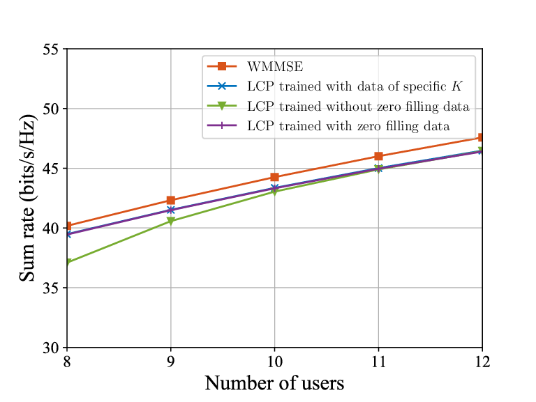
Fig 8 presents the user number generalization performance of the proposed method under different training settings, where the abscissa represents the actual number of users in the system. For a specific number of users , three training settings are considered, including 1) trained with data of specific : training a model with , testing on ; 2) trained without zero filling data: training a model with , testing on and ; 3) trained with zero filling data: training a model with and , testing on and . For the WMMSE algorithm, it can naturally adapt to the zero filling input, so it maintains nearly optimal performance, and thus can be used as a performance baseline of generalization ability. For the proposed algorithm, when the training data does not contain zero filling data, the network can not adapt to the input of zero filling data, the performance decreased obviously. Fortunately, with the help of zero filling data for training, it can be seen that the model trained on zero filling data achieves almost the same performance with the customized model trained on specific data, and a close performance to the WMMSE algorithm, which shows its strong generalization ability on number of users. In conclusion, the data-driven method should try to make the training data and test data have similar statistical characteristics. Once the proposed scheme has partial zero filling data samples for auxiliary training, the generalization ability can be greatly improved.
VI-E3 Imperfect CSI
Fig. 9 shows the performance of the four precoding schemes with imperfect CSI, where the precoding matrix is designed based on the noisy channel, i.e., , and the actual sum rate is calculated based on the noiseless channel . For WMMSE algorithm and EZF algorithm, their performance drops a lot due to the strong dependence on the accurate channel. For the proposed LCP algorithm, it can adapt to such noise through a large number of training samples in the offline training stage, so as to performance better. Though the LUW algorithm, another learning based scheme, enjoys such adaptive process as well, the proposed LCP algorithm outperforms the LUW algorithm in all the error settings. With the decrease of channel estimation error, the channel becomes relatively more accurate, the WMMSE algorithm leads the performance again at the cost of huge computational complexity, but still the proposed LCP algorithm has a close performance with the WMMSE algorithm, which demonstrates the robustness of the proposed LCP algorithm in imperfect CSI scenarios.

VI-F Precoding with Granularity of Multi-RB Channels


Fig 10 shows the sum rate performance of the four precoding schemes when the precoding granularity . It can be found that in the two system setting cases, the WMMSE algorithm, still leads the performance. For the proposed LCP algorithm, it achieves nearly 90% performance of WMMSE algorithm, while has much lower computational complexity. Moreover, compared with EZF and LUW algorithm which has a similar computational complexity, LCP algorithm significantly outperforms them in the sum-rate performance. It can be concluded that the proposed LCP algorithm has good practicability in MIMO-OFDM system.

Fig 11 shows the sum rate performance of the four schemes in different precoding granularity, where the sum rate is divided by the precoding granularity . When increases, there are more RB that needs to share a common precoding matrix, the precoding algorithm needs to take all of them into account, and thus the per RB’s sum-rate decreases. It can be found that the proposed LCP algorithm outperforms the LUW algorithm and the EZF algorithm a lot, and still has the closest performance to WMMSE algorithm. The performance gap between the proposed LCP algorithm and WMMSE algorithm increases with the increase of . This is because when increases, the key feature has a greater impact on the performance, and the learning performance of neural network drops due to the more complex mapping from the channel to . This problem can be solved by designing a more effective network, which is worthy of further study to promote the application of the proposed algorithm in the practical system.
VII Conclusion
In this paper, we have proposed a novel data-driven precoding algorithm. Firstly, we develop a method to transform the MIMO precoding problem into MISO precoding problem. Then, we present a DL-based solution for the corresponding MISO precoding problem, and further reduce the complexity through recovery module compression and model pruning. The extension to the MIMO-OFDM systems is also discussed. Experimental results show that the proposed scheme achieves similar performance with the WMMSE algorithm, and has a much lower computational cost. For future work, it is interesting to extend the proposed scheme to hybrid precoding scenarios and multi-cell systems.
-A Proof of Proposition 2
Proof: From (7), it can be found that is determined by the final , where denotes the number of iterations to convergence. Therefore, to establish proposition 2, we only needs to prove that is determined by . For convenience of expression, we use to denote that is a function of .
With the intermediate variable , the WMMSE algorithm obtains by performing the following three steps.
| (22) | ||||
| (23) | ||||
| (24) |
where , .
Let , , , . Then can be expressed as
| (25) |
where .
Then we have
| (26) | ||||
| (27) | ||||
| (28) |
From the definition of , we have
| (29) |
Moreover, can be expressed as
| (30) |
where is the element of row and column of .
-B Proof of Proposition 3
The WSR maximization problem in MISO scenario is given as follows.
| (33) | ||||
| (34) |
Then the weighted least mean square error problem can be formulated as
| (35) |
where is given by
| (36) |
Similar to [2] and [3], it can be proven that and is equivalent. Therefore, we can obtain the iterative based solution for by solving as follows.
| (37) | ||||
| (38) | ||||
| (39) |
Therefore, the optimal precoding matrix should meet the form of (39). Proposition 3 can be obtained by reorganizing (39), which ends the proof.
References
- [1] S. S. Christensen, R. Agarwal, E. De Carvalho, and J. M. Cioffi, “Weighted sum-rate maximization using weighted MMSE for MIMO-BC beamforming design,” IEEE Trans. Wireless Commun., vol. 7, no. 12, pp. 4792–4799, 2008.
- [2] Q. Shi, M. Razaviyayn, Z.-Q. Luo, and C. He, “An iteratively weighted MMSE approach to distributed sum-utility maximization for a MIMO interfering broadcast channel,” IEEE Trans. Singal Process., vol. 59, no. 9, pp. 4331–4340, 2011.
- [3] Q. Hu, Y. Cai, Q. Shi, K. Xu, G. Yu, and Z. Ding, “Iterative algorithm induced deep-unfolding neural networks: Precoding design for multiuser MIMO systems,” IEEE Trans. Wireless Commun., 2020.
- [4] S. Lu, S. Zhao, and Q. Shi, “Learning-based massive beamforming,” in Proc. IEEE Global Communications Conference (GLOBECOM), pp. 1–6, Taipei, Taiwan, 2020.
- [5] G. Caire and S. Shamai, “On the achievable throughput of a multiantenna Gaussian broadcast channel,” IEEE Trans Inf. Theory, vol. 49, no. 7, pp. 1691–1706, 2003.
- [6] Q. H. Spencer, A. L. Swindlehurst, and M. Haardt, “Zero-forcing methods for downlink spatial multiplexing in multiuser MIMO channels,” IEEE Trans. Singal Process., vol. 52, no. 2, pp. 461–471, 2004.
- [7] T. Yoo and A. Goldsmith, “On the optimality of multiantenna broadcast scheduling using zero-forcing beamforming,” IEEE J. Sel. Areas Commun., vol. 24, no. 3, pp. 528–541, 2006.
- [8] L. Sun and M. R. McKay, “Eigen-based transceivers for the MIMO broadcast channel with semi-orthogonal user selection,” IEEE Trans. Singal Process., vol. 58, no. 10, pp. 5246–5261, 2010.
- [9] C. B. Peel, B. M. Hochwald, and A. L. Swindlehurst, “A vector-perturbation technique for near-capacity multiantenna multiuser communication-part I: channel inversion and regularization,” IEEE Trans. Commun., vol. 53, no. 1, pp. 195–202, 2005.
- [10] S. Lu, S. Zhao, and Q. Shi, “Block-diagonal zero-forcing beamforming for weighted sum-rate maximization in multi-user massive MIMO systems,” in Proc. IEEE Symposium on Computers and Communications (ISCC), pp. 1–6, Rennes, France, 2020.
- [11] C. Zhang, Y. Jing, Y. Huang, and L. Yang, “Performance analysis for massive MIMO downlink with low complexity approximate zero-forcing precoding,” IEEE Trans. Commun., vol. 66, no. 9, pp. 3848–3864, 2018.
- [12] H. Sun, X. Chen, Q. Shi, M. Hong, X. Fu, and N. D. Sidiropoulos, “Learning to optimize: Training deep neural networks for interference management,” IEEE Trans. Singal Process., vol. 66, no. 20, pp. 5438–5453, 2018.
- [13] H. Ye, G. Y. Li, and B.-H. F. Juang, “Deep reinforcement learning based resource allocation for V2V communications,” IEEE Trans. Veh. Technol., vol. 68, no. 4, pp. 3163–3173, 2019.
- [14] L. Liang, H. Ye, and G. Y. Li, “Spectrum sharing in vehicular networks based on multi-agent reinforcement learning,” IEEE J. Sel. Areas Commun., vol. 37, no. 10, pp. 2282–2292, 2019.
- [15] L. Liang, H. Ye, G. Yu, and G. Y. Li, “Deep-learning-based wireless resource allocation with application to vehicular networks,” Proc. IEEE, vol. 108, no. 2, pp. 341–356, 2019.
- [16] M. Eisen, C. Zhang, L. F. Chamon, D. D. Lee, and A. Ribeiro, “Learning optimal resource allocations in wireless systems,” IEEE Trans. Singal Process., vol. 67, no. 10, pp. 2775–2790, 2019.
- [17] H. Ye, G. Y. Li, and B.-H. Juang, “Power of deep learning for channel estimation and signal detection in OFDM systems,” IEEE Wireless Commun. Lett., vol. 7, no. 1, pp. 114–117, 2017.
- [18] N. Samuel, T. Diskin, and A. Wiesel, “Learning to detect,” IEEE Trans. Singal Process., vol. 67, no. 10, pp. 2554–2564, 2019.
- [19] H. He, C.-K. Wen, S. Jin, and G. Y. Li, “Model-driven deep learning for MIMO detection,” IEEE Trans. Singal Process., vol. 68, pp. 1702–1715, 2020.
- [20] H. He, C.-K. Wen, S. Jin, and G. Y. Li, “Deep learning-based channel estimation for beamspace mmWave massive MIMO systems,” IEEE Wireless Commun. Lett., vol. 7, no. 5, pp. 852–855, 2018.
- [21] P. Dong, H. Zhang, G. Y. Li, I. S. Gaspar, and N. NaderiAlizadeh, “Deep CNN-based channel estimation for mmWave massive MIMO systems,” IEEE J. Sel. Topics Signal Process., vol. 13, no. 5, pp. 989–1000, 2019.
- [22] X. Ma and Z. Gao, “Data-driven deep learning to design pilot and channel estimator for massive MIMO,” IEEE Trans. Veh. Technol., vol. 69, no. 5, pp. 5677–5682, 2020.
- [23] Y. Yang, F. Gao, C. Xing, J. An, and A. Alkhateeb, “Deep multimodal learning: Merging sensory data for massive MIMO channel prediction,” IEEE J. Sel. Areas Commun., 2020.
- [24] J. Gao, M. Hu, C. Zhong, G. Y. Li, and Z. Zhang, “An attention-aided deep learning framework for massive MIMO channel estimation,” IEEE Trans. Wireless Commun., 2021.
- [25] J. Gao, C. Zhong, X. Chen, H. Lin, and Z. Zhang, “Unsupervised learning for passive beamforming,” IEEE Commun. Lett., vol. 24, no. 5, pp. 1052–1056, 2020.
- [26] H. Song, M. Zhang, J. Gao, and C. Zhong, “Unsupervised Learning-Based Joint Active and Passive Beamforming Design for Reconfigurable Intelligent Surfaces Aided Wireless Networks,” IEEE Commun. Lett., vol. 25, no. 3, pp. 892–896, 2020.
- [27] L. Pellaco, M. Bengtsson, and J. Jaldén, “Deep unfolding of the weighted MMSE beamforming algorithm,” [Online]. Available: https://arxiv.org/abs/2006.08448, 2020.
- [28] H. Huang, W. Xia, J. Xiong, J. Yang, G. Zheng, and X. Zhu, “Unsupervised learning-based fast beamforming design for downlink MIMO,” IEEE Access, vol. 7, pp. 7599–7605, 2018.
- [29] W. Xia, G. Zheng, Y. Zhu, J. Zhang, J. Wang, and A. P. Petropulu, “A deep learning framework for optimization of MISO downlink beamforming,” IEEE Trans. Commun., vol. 68, no. 3, pp. 1866–1880, 2019.
- [30] J. Kim, H. Lee, S.-E. Hong, and S.-H. Park, “Deep learning methods for universal MISO beamforming,” IEEE Wireless Commun. Lett., vol. 9, no. 11, pp. 1894–1898, 2020.
- [31] H. He, S. Jin, C.-K. Wen, F. Gao, G. Y. Li, and Z. Xu, “Model-driven deep learning for physical layer communications,” IEEE Wireless Commun., vol. 26, no. 5, pp. 77–83, 2019.
- [32] A. Zappone, M. Di Renzo, and M. Debbah, “Wireless networks design in the era of deep learning: Model-based, AI-based, or both?,” IEEE Trans. Commun., vol. 67, no. 10, pp. 7331–7376, 2019.
- [33] W. Yu and T. Lan, “Transmitter optimization for the multi-antenna downlink with per-antenna power constraints,” IEEE Trans. Singal Process., vol. 55, no. 6, pp. 2646–2660, 2007.
- [34] E. Björnson, M. Bengtsson, and B. Ottersten, “Optimal multiuser transmit beamforming: A difficult problem with a simple solution structure [lecture notes],” IEEE Signal Process. Mag., vol. 31, no. 4, pp. 142–148, 2014.
- [35] M. Chen, U. Challita, W. Saad, C. Yin, and M. Debbah, “Artificial neural networks-based machine learning for wireless networks: A tutorial,” IEEE Commun. Surveys & Tutorials, vol. 21, no. 4, pp. 3039–3071, 2019.
- [36] L. D. Nguyen, H. D. Tuan, T. Q. Duong, and H. V. Poor, “Multi-user regularized zero-forcing beamforming,” IEEE Trans. Singal Process., vol. 67, no. 11, pp. 2839–2853, 2019.
- [37] H. Li, A. Kadav, I. Durdanovic, H. Samet, and H. P. Graf, “Pruning filters for efficient convnets,” [Online]. Available: https://arxiv.org/abs/1608.08710, 2016.
- [38] Y. He, G. Kang, X. Dong, Y. Fu, and Y. Yang, “Soft filter pruning for accelerating deep convolutional neural networks,” [Online]. Available: https://arxiv.org/abs/1808.06866, 2018.
- [39] 3GPP, “NR; NR and NG-RAN Overall Description,” Technical Specification (TS) 38.300, 3rd Generation Partnership Project (3GPP), 2021.
- [40] Z. Zhou, J. Fang, L. Yang, H. Li, Z. Chen, and R. S. Blum, “Low-rank tensor decomposition-aided channel estimation for millimeter wave MIMO-OFDM systems,” IEEE J. Sel. Areas Commun., vol. 35, no. 7, pp. 1524–1538, 2017.