Bounding Box Disparity: 3D Metrics for Object Detection
With Full Degree of Freedom

Michael G. Adam Martin Piccolrovazzi Sebastian Eger Eckehard Steinbach Thanks: This work is funded by Germany’s Federal Ministry of Education and Research within the project KIMaps (grant ID #01IS20031C).

Abstract

The most popular evaluation metric for object detection in 2D images is Intersection over Union (IoU). Existing implementations of the IoU metric for 3D object detection usually neglect one or more degrees of freedom. In this paper, we first derive the analytic solution for three dimensional bounding boxes. As a second contribution, a closed-form solution of the volume-to-volume distance is derived. Finally, the Bounding Box Disparity is proposed as a combined positive continuous metric. We provide open source implementations of the three metrics as standalone python functions, as well as extensions to the Open3D library and as ROS nodes.

Index Terms:

metric, object detection, 3D bounding box, intersection over union, volume-to-volume distance

^†^†address: Chair of Media Technology and Munich Institute of Robotics and Machine Intelligence,
Technical University of Munich, Munich, Germany

1 Introduction

As 3D object detection gets more popular and new datasets are published [1, 2, 3], evaluation metrics gain in importance. The most common one is Intersection over Union (IoU). It is well known from object detection on two-dimensional data such as images. Existing implementations of its three-dimensional counterpart usually neglect one or more degrees of freedom. Examples for this are implementations that work with axis-aligned bounding boxes or only consider a rotation around the z-axis [4]. This oversimplifies real world problems, as usually rotation of objects is possible in any given direction.
To the best of our knowledge, although the strategy of computing IoU has already been mathematically generalized [5], we provide and derive the first closed-form analytic solution for the case of 3D bounding boxes with full degree of freedom.
We further derive an analytic solution for the volume-to-volume distance (v2v) of two 3D bounding boxes. The metric v2v is defined as the shortest distance between the hull of one volume to the hull of another volume. Both metrics are visualized in Fig. 1.
For both metrics we provide the first open source implementation as a standalone python function, as well as an extension to the Open3D library [6] and a ROS-node [7].
This paper is structured as follows. First, we discuss related work. In Section 3, we mathematically define bounding boxes and review the existing metrics. Afterwards the solution for volumetric IoU is stated and shortly compared to its point based method. Consecutively v2v is presented and a combined positive continuous metric called Bounding Box Disparity (BBD) is proposed.

2 Related work

Calculating the intersection of two three-dimensional volumes is a common task in rendering, CAD pipelines and deep learning [8]. In open source frameworks such as blender [9] it is possible to use an accurate solver. In practice, fast numerical solutions are used, in order to speed up the computation with the disadvantage of loosing accuracy. Instead of using cuboids directly, the frameworks usually have in common that only triangular-mesh representations are allowed for boolean operations such as intersection.
Hence, with an additional step of meshifying bounding boxes one can define a volumetric intersection. This adds unnecessary computation of multiple equations and conversions. For reference purposes, we also provide a blender-based implementation of this method. When used for custom code this adds a big dependency, since blender and its API is rather developed for graphical usage with complex scenes, but not for calculating basic linear equations.
The Open3D framework, which is often used in the context of machine learning does not have an implementation of an exact intersection for meshes, as well as no solution for oriented bounding boxes.
Benchmarks for 3D object detection such as [10] often rely on evaluation metrics that use axis aligned bounding boxes or bounding boxes with only a rotation around the z-axis [11, 12]. Other benchmarks like [13] use a combination of 2D IoU and an additional orientation value. To the best of our knowledge there are no full-degree of freedom bounding box benchmarks published for the 3D case yet.

3 Methods

3.1 Definition of a Bounding Box

First, we have to define a bounding box $i$ , shown in Fig. 2. It can be represented by a transformation matrix $T^{i}$ , consisting of its rotation $R^{i}$ , position $p^{i}$ and dimension $d^{i}$

T^{i}=\left[\begin{array}[]{c|c}\scalebox{1.2}{$d^{i}R^{i}$}&\scalebox{1.2}{$p^{i}$}\\ \hline\cr 0\;0\;0&1\end{array}\right],

(1)

whereas the position corresponds to the cuboid center. Its corners $C_{1-8}^{i}$ can then be defined as follows:

C_{1-8}^{i}=T^{i}u_{1-8}

(2)

with $u_{1-8}$ being defined as the corners of the unit cube centered around the origin of the coordinate system.

$u_{1-8}=\begin{bmatrix}-0.5&0.5&-0.5&-0.5&0.5&-0.5&0.5&0.5\\ -0.5&-0.5&0.5&-0.5&0.5&0.5&-0.5&0.5\\ -0.5&-0.5&-0.5&0.5&0.5&0.5&0.5&-0.5\end{bmatrix}$

(3)

One can further define the edges $e_{1-12}^{i}$ and faces $f_{1-6}^{i}$ of a cube as a list of connected corners. Its elements correspond to the column-index in the matrix of corners.

$\displaystyle e_{1-12}=$	$\displaystyle[[1,2],[2,8],[3,8],[1,3],[4,7],[7,5],$
	$\displaystyle[6,5],[4,6],[1,4],[2,7],[8,5],[3,6]]$	(4)
$\displaystyle f_{1-12}=$	$\displaystyle[[1,2,3],[1,2,4],[1,3,4],$
	$\displaystyle[5,6,7],[5,6,8],[5,7,8]]$	(5)

Lastly, the normal vectors $n_{1-6}^{i}$ of the faces are defined by the rotation $R^{i}$ . Each column $r_{j}^{i}$ corresponds to two face normals - one time in positive and one time in negative direction.

$\displaystyle R^{i}$	$\displaystyle=[r_{1}^{i},r_{2}^{i},r_{3}^{i}]$
$\displaystyle n_{1}^{i}$	$\displaystyle=-r_{3}^{i}\qquad n_{2}^{i}=-r_{2}^{i}\qquad n_{3}^{i}=-r_{1}^{i}$	(6)
$\displaystyle n_{4}^{i}$	$\displaystyle=+r_{3}^{i}\qquad n_{5}^{i}=+r_{2}^{i}\qquad n_{6}^{i}=+r_{1}^{i}$

3.2 Metrics

There a several metrics to consider when comparing two bounding boxes (BB) [14, 15]:

•

absolute/quadratic difference in position
•

absolute/quadratic difference in size
•

rotation (can affect difference in size [16]), i.e.:

- angular-difference of euler angles

- quaternion-distance

- distance of rotation matrices
•

IoU of point-cloud points within the BBs [17]
•

volumetric IoU
•

volume-to-volume distance

All of the above are part of our open source implementation. Only the last two are discussed in the following.

3.3 Volumetric IoU

3.3.1 Points of interest

We now define possible corner points $POI$ of the intersection. There are four candidates:

•

Corners of the first cuboid laying inside the second cuboid
•

Corners of the second cuboid laying inside the first cuboid
•

Intersections of an edge of the first cuboid with a plane of the second cuboid
•

Intersections of an edge of the second cuboid with a plane of the first cuboid

In order to compute them, we formulate equations for each line and plane corresponding to the edges and faces of both cubes. The lines can simply be defined as

L_{k}^{i}\left(t_{l}\right)=e_{k,1}^{i}+\underbrace{\left(e_{k,2}^{i}-e_{k,1}^{i}\right)}_{\begin{subarray}{c}m_{k}^{i}\end{subarray}}t_{l}

(7)

with $m_{k}^{i}$ describing the line’s slope. Whereas the planes can be defined by three corner points.

\displaystyle P_{k}^{i}\left(t_{p}\right)=f_{k,1}^{i}+\underbrace{\begin{bmatrix}f_{k,2}^{i}-f_{k,1}^{i}&f_{k,3}^{i}-f_{k,1}^{i}\end{bmatrix}}_{\begin{subarray}{c}N_{k}^{i}\end{subarray}}\begin{bmatrix}t_{p,1}\\ t_{p,2}\end{bmatrix}

(8)

The $3\times 2$ -matrix $N_{k}^{i}$ can also be expressed by the normals perpendicular to the face normal $n_{k}^{i}$ scaled according to $d^{i}$ .
For all possible line-plane combinations of the two cuboids, we get $144$ equations. Each resulting in possible points of interest. The number depends on how many lines are parallel with the planes or lay in the planes. This again depends on how the cubes are rotated to each other.
Next, we calculate the corners $C^{1},C^{2}$ of both cuboids and add them to the list of points.

3.3.2 Checking Validity of the Points

Now every point in the solution list has to be checked, if its a valid corner point of the intersection. For this the points have to be part of both cubes.
This can be done by transforming the points into the coordinate system of $T^{1}$ .

POI={T^{1}}^{-1}POI

(9)

The corner points of the first cube $C_{1}$ now correspond to the ones of a unit cube $u_{1-8}$ . Thus, every point has to be checked if its coordinates are smaller than $0.5$ and greater than $-0.5$ .

valid=(POI<0.5)\,\&\,(POI>-0.5)

(10)

After pruning the non valid points from the list, we transform everything into the coordinate system of the second cube $T^{2}$ .

POI={T^{2}}^{-1}T^{1}POI

(11)

Repeating the validity check from equation 10 leaves us all relevant points.

3.3.3 Calculating the Volume

We now pick every valid point and construct the convex hull of this set of points, which corresponds to the intersection of the cuboids. If the hull cannot be constructed, because no point is valid or the points all lay in a plane, then there is no intersection, thus $IoU=0$ holds.
In all other cases, the volume of the hull $V_{I}$ can be computed by summation of the signed volumes of tetrahedrons [18].
As a last step we calculate the volume of the union $V_{U}$

V_{U}=d_{1}^{1}d_{2}^{1}d_{3}^{1}+d_{1}^{2}d_{2}^{2}d_{3}^{2}-V_{I}

(12)

such that $IoU$ is defined as

IoU=\frac{V_{I}}{V_{U}}.

(13)

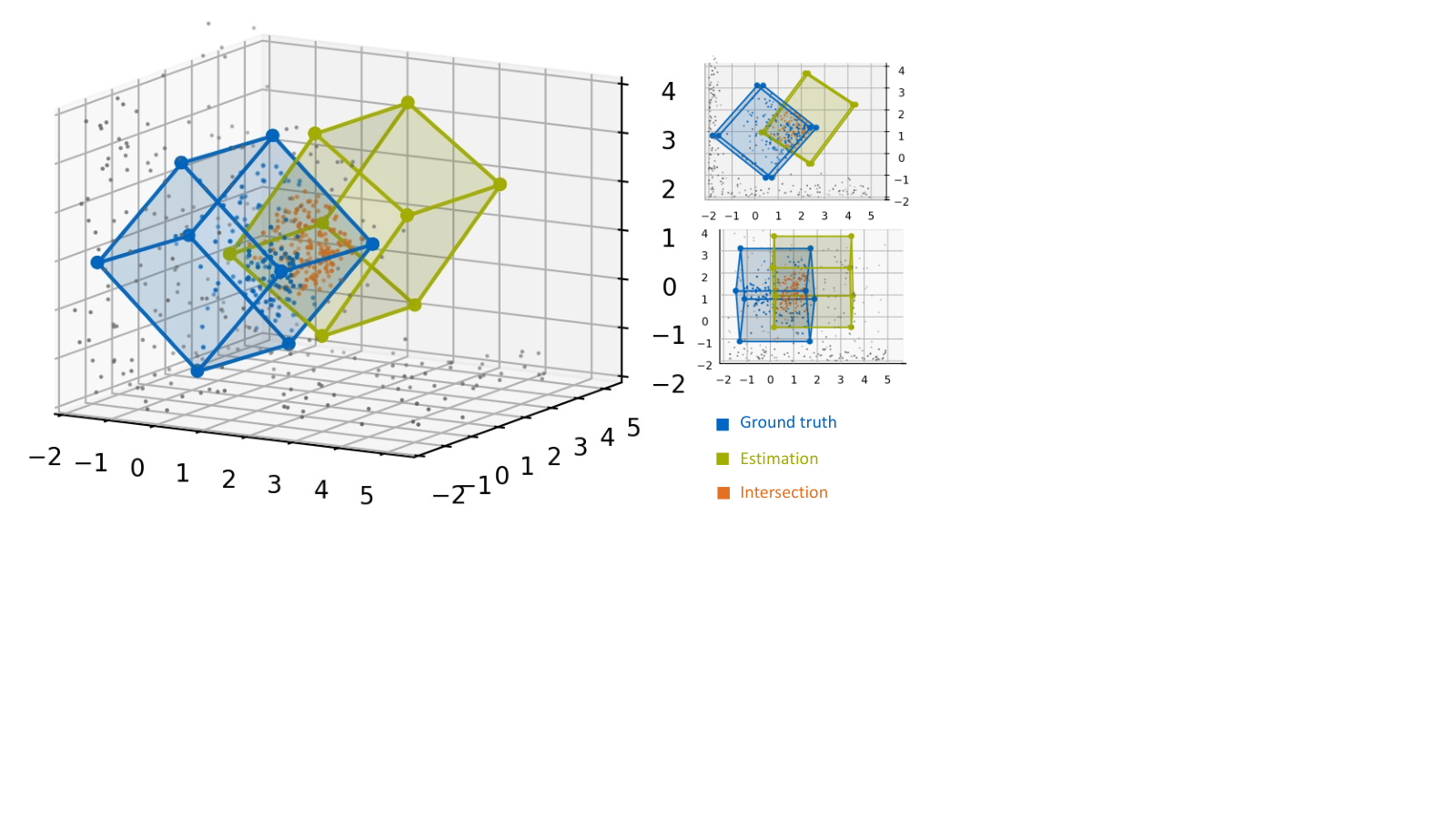
3.4 Comparison of point and volume based IoU

In Fig 3 a typical example of an object leaning against a wall is shown. The underlying point cloud is constructed by a lidar scan. Hence, most of the points of the object lay in the front. With the shown estimation of an object detector, this results in a relatively high intersection over union of $0.47$ , when computed based on the points in the cloud, in comparison to $0.07$ of the semantically more meaningful volumetric counterpart.

3.5 Volume-to-Volume Distance

3.5.1 Point-Pairs of Interest

Similar to calculating the volumetric IoU, point-pairs of interest (PPOIs) can be defined, one of which gives the shortest distance $d_{s}$ between two bounding boxes $T^{1}$ , $T^{2}$ such that

	$\displaystyle d_{s}=\textit{norm}(P^{1}_{s}-P^{2}_{s})<\textit{norm}(P^{1}_{i}-P^{2}_{j}),$			(14)
	$\displaystyle i\in\textit{hull}(T^{1})\,\&\,j\in\textit{hull}(T^{2})$

Where $P^{1}_{s}$ , $P^{2}_{s}$ denotes the two points from where the shortest distance is measured. Notice that the surface of the bounding boxes is an infinite, non discrete set of points, however, only a discrete set of points can be candidates for the pair of $P_{s}$ .
The relevant point-pairs, shown in Fig 4, are as follows

•

Corners of the first cuboid with their rectangular projection on the faces of the second cuboid (a)
•

Corners of the second cuboid with their rectangular projection on the faces of the first cuboid
•

Corners of the first cuboid with their rectangular projection on the edges of the second cuboid (b)
•

Corners of the second cuboid with their rectangular projection on the edges of the first cuboid
•

The distance defined by two edges, each of one cube (c)
•

The distance defined by two corners, each of one cube (d)

In order to compute the point-pairs and the corresponding distances, we formulate equations for each point-face, point-edge, edge-edge projections.

3.5.2 Point-Plane Projection

The shortest distance $d$ between a point and a plane is given by its projection. In case of corners $l$ of one cuboid $i$ and the faces $k$ of another cuboid $j$ , it is defined by

$\displaystyle v$	$\displaystyle=C_{l}^{i}-f_{k,0}^{j}$	(15)
$\displaystyle d$	$\displaystyle={n_{k}^{j}}^{T}v$	(16)
$\displaystyle p_{\textit{prj}}$	$\displaystyle=C_{l}^{i}+n_{k}^{j}*d$	(17)

In order to check if the projected point $p_{\textit{prj}}$ is within the face $f_{k}^{j}$ of the cube $j$ one can calculate the parameters $t_{p,1}$ and $t_{p,2}$ of its plane-function $P_{k}^{j}$ . This can be done by calculating the pseudo-inverse of $N_{k}^{j}$ .

\begin{bmatrix}t_{p,1}\\ t_{p,2}\end{bmatrix}=\left({N_{k}^{j}}^{T}N_{k}^{j}\right)^{-1}N_{k}^{j}\;v={N_{k}^{j}}^{+}\;v

(18)

Only if both parameters are between $0$ and $1$ , the projected point is a valid point.

3.5.3 Point-Line projection

The shortest distance $d$ between a point and a line is given by its projection. In case of corners $l$ of one cuboid $i$ and the edges $k$ of another cuboid $j$ , it is defined by

	$\displaystyle t$	$\displaystyle=\frac{\left(C_{l}^{i}-l_{k,0}^{j}\right)^{T}m_{k}^{j}}{{m_{k}^{j}}^{2}}$		(19)
	$\displaystyle p_{\textit{prj}}$	$\displaystyle=L_{k}^{j}(t)$		(20)

Only if parameter $t$ has a value between $0$ and $1$ , the projected point is a valid point. The solution is only defined for non-parallel lines, which in our case is sufficient. In parallel cases, the shortest distance is already given by the point to point or point to edge distance.

3.5.4 Line-Line projection

The shortest distance $d$ between a line and another line is given by its projection. In case of edges $k$ of one cuboid $i$ and the edges $l$ of another cuboid $j$ , it is defined by

$\displaystyle v$	$\displaystyle=e_{k}^{i}-e_{l}^{j}$	(21)
$\displaystyle det$	$\displaystyle={m_{k}^{i}}^{2}+{m_{l}^{j}}^{2}+{m_{k}^{i}}^{T}m_{l}^{j}$	(22)
$\displaystyle t^{i}$	$\displaystyle=\frac{{m_{l}^{j}}^{2}\left({m_{k}^{i}}^{T}v\right)-\left({m_{l}^{j}}^{T}v\right)\left({m_{k}^{i}}^{T}m_{l}^{j}\right)}{det}$	(23)

$\displaystyle t^{j}$	$\displaystyle=\frac{-{m_{k}^{i}}^{2}\left({m_{l}^{j}}^{T}v\right)+\left({m_{k}^{i}}^{T}v\right)\left({m_{k}^{i}}^{T}m_{l}^{j}\right)}{det}$	(24)
$\displaystyle p_{\textit{prj}}^{i}$	$\displaystyle=L_{k}^{i}(t^{i})$	(25)
$\displaystyle p_{\textit{prj}}^{j}$	$\displaystyle=L_{l}^{j}(t^{j})$	(26)

The formula for the parameters $t^{i},t^{j}$ can be derived by solving the minimization-problem $\left(L_{k}^{i}-L_{l}^{j}\right)^{2}$ .

3.5.5 Shortest Distance

Every combination results in a maximum of $496$ point-pairs of interest. Since all functions only consist of linear equations, efficient methods of parallel computing can be applied. As a last step left, one must sort the list of candidates according to a vector-norm, such as L2 of the point-pair difference. Using L2 has the advantage that the values are already byproducts of the previously introduced point-to-plane projection. The shortest value of all PPOIs then corresponds to the shortest volume-to-volume distance.

3.6 Bounding Box Disparity

As a last metric we introduce the bounding box disparity (BBD), which is a combination of IoU and v2v. Since the Intersection over Union can only rank the similarity of two bounding boxes when they are overlapping, a distinction between two bounding boxes closer or farther away without an overlap cannot be made. Hence, we suggest the combination of IoU and v2v in the following way

BBD=1-IoU+v2v

(27)

such that a continuous positive metric for the (dis-)similarity of two bounding boxes can be calculated. IoU can have values between $0$ and $1$ , whereas $1$ corresponds to a total match and $0$ to no overlap. v2v on the other hand is $0$ as long as there is overlap and increases with further distance/mismatch of the bounding boxes. This results in a first quickly, but then linearly increasing scalar-field $BBD$ .

4 Conclusion

With this paper we publish an open source library¹¹ 1 https://github.com/M-G-A/3D-Metrics for multiple 3D metrics for object detection, including the first analytic solution and its implementation of volumetric Intersection over Union and volume-to-volume distance for two bounding boxes with full degree of freedom. Further, we introduce the combined metric Bounding Box Disparity. In future work this could be extended such that for non overlapping bounding boxes also the rotation and size differences are considered.

References

[1] Santhosh K. Ramakrishnan, Aaron Gokaslan, Erik Wijmans, Oleksandr Maksymets, Alex Clegg, John Turner, Eric Undersander, Wojciech Galuba, Andrew Westbury, and Angel X. Chang, “Habitat-Matterport 3D Dataset (HM3D): 1000 Large-scale 3D Environments for Embodied AI,” arXiv preprint arXiv:2109.08238, 2021.
[2] Gilad Baruch, Zhuoyuan Chen, Afshin Dehghan, Tal Dimry, Yuri Feigin, Peter Fu, Thomas Gebauer, Brandon Joffe, Daniel Kurz, and Arik Schwartz, “ARKitScenes–A Diverse Real-World Dataset For 3D Indoor Scene Understanding Using Mobile RGB-D Data,” arXiv preprint arXiv:2111.08897, 2021.
[3] Artsiom Ablavatski Jianing Wei Matthias Grundmann Adel Ahmadyan, Liangkai Zhang, “Objectron: A large scale dataset of object-centric videos in the wild with pose annotations,” Proceedings of the IEEE Conference on Computer Vision and Pattern Recognition, 2021.
[4] Jun Xu, Yanxin Ma, Songhua He, and Jiahua Zhu, “3D-GIoU: 3D generalized intersection over union for object detection in point cloud,” Sensors, vol. 19, no. 19, pp. 4093, 2019, Publisher: Multidisciplinary Digital Publishing Institute.
[5] Ivan E. Sutherland and Gary W. Hodgman, “Reentrant polygon clipping,” Communications of the ACM, vol. 17, no. 1, pp. 32–42, 1974, Publisher: ACM New York, NY, USA.
[6] Qian-Yi Zhou, Jaesik Park, and Vladlen Koltun, “Open3D: A modern library for 3D data processing,” arXiv:1801.09847, 2018.
[7] Morgan Quigley, Ken Conley, Brian Gerkey, Josh Faust, Tully Foote, Jeremy Leibs, Rob Wheeler, and Andrew Y. Ng, “ROS: an open-source Robot Operating System,” in ICRA workshop on open source software. 2009, vol. 3, p. 5, Kobe, Japan, Issue: 3.2.
[8] Yana Hasson, Gul Varol, Dimitrios Tzionas, Igor Kalevatykh, Michael J. Black, Ivan Laptev, and Cordelia Schmid, “Learning joint reconstruction of hands and manipulated objects,” in Proceedings of the IEEE/CVF Conference on Computer Vision and Pattern Recognition, 2019, pp. 11807–11816.
[9] Blender Online Community, Blender - a 3D modelling and rendering package, http://www.blender.org, Blender Foundation, Blender Institute, Amsterdam.
[10] I. Armeni, A. Sax, A. R. Zamir, and S. Savarese, “Joint 2D-3D-Semantic Data for Indoor Scene Understanding,” ArXiv e-prints, Feb. 2017.
[11] Shuran Song, Samuel P Lichtenberg, and Jianxiong Xiao, “Sun rgb-d: A rgb-d scene understanding benchmark suite,” in Proceedings of the IEEE conference on computer vision and pattern recognition, 2015, pp. 567–576.
[12] Angela Dai, Angel X Chang, Manolis Savva, Maciej Halber, Thomas Funkhouser, and Matthias Nießner, “Scannet: Richly-annotated 3d reconstructions of indoor scenes,” in Proceedings of the IEEE conference on computer vision and pattern recognition, 2017, pp. 5828–5839.
[13] Andreas Geiger, Philip Lenz, and Raquel Urtasun, “Are we ready for autonomous driving? the kitti vision benchmark suite,” in 2012 IEEE conference on computer vision and pattern recognition. 2012, pp. 3354–3361, IEEE.
[14] Caner Sahin, Guillermo Garcia-Hernando, Juil Sock, and Tae-Kyun Kim, “A review on object pose recovery: from 3d bounding box detectors to full 6d pose estimators,” Image and Vision Computing, vol. 96, pp. 103898, 2020, Publisher: Elsevier.
[15] Arsalan Mousavian, Dragomir Anguelov, John Flynn, and Jana Kosecka, “3d bounding box estimation using deep learning and geometry,” in Proceedings of the IEEE conference on Computer Vision and Pattern Recognition, 2017, pp. 7074–7082.
[16] Danila Rukhovich, Anna Vorontsova, and Anton Konushin, “FCAF3D: Fully Convolutional Anchor-Free 3D Object Detection,” arXiv preprint arXiv:2112.00322, 2021.
[17] Zetong Yang, Yanan Sun, Shu Liu, Xiaoyong Shen, and Jiaya Jia, “Std: Sparse-to-dense 3d object detector for point cloud,” in Proceedings of the IEEE/CVF International Conference on Computer Vision, 2019, pp. 1951–1960.
[18] Cha Zhang and Tsuhan Chen, “Efficient feature extraction for 2d/3d objects in mesh representation,” in Proceedings 2001 International Conference on Image Processing (Cat. No. 01CH37205). IEEE, 2001, vol. 3, pp. 935–938.

Bounding Box Disparity: 3D Metrics for Object Detection With Full Degree of Freedom