Balanced Self-Paced Learning for AUC Maximization

Abstract

Learning to improve AUC performance is an important topic in machine learning. However, AUC maximization algorithms may decrease generalization performance due to the noisy data. Self-paced learning is an effective method for handling noisy data. However, existing self-paced learning methods are limited to pointwise learning, while AUC maximization is a pairwise learning problem. To solve this challenging problem, we innovatively propose a balanced self-paced AUC maximization algorithm (BSPAUC). Specifically, we first provide a statistical objective for self-paced AUC. Based on this, we propose our self-paced AUC maximization formulation, where a novel balanced self-paced regularization term is embedded to ensure that the selected positive and negative samples have proper proportions. Specially, the sub-problem with respect to all weight variables may be non-convex in our formulation, while the one is normally convex in existing self-paced problems. To address this, we propose a doubly cyclic block coordinate descent method. More importantly, we prove that the sub-problem with respect to all weight variables converges to a stationary point on the basis of closed-form solutions, and our BSPAUC converges to a stationary point of our fixed optimization objective under a mild assumption. Considering both the deep learning and kernel-based implementations, experimental results on several large-scale datasets demonstrate that our BSPAUC has a better generalization performance than existing state-of-the-art AUC maximization methods.

Introduction

Learning to improve AUC performance is an important topic in machine learning, especially for imbalanced datasets (Huang and Ling 2005; Ling, Huang, and Zhang 2003; Cortes and Mohri 2004). Specifically, for severely imbalanced binary classification datasets, a classifier may achieve a high prediction accuracy if it predicts all samples to be the dominant class. However, the classifier actually has a poor generalization performance because it cannot properly classify samples from non-dominant class. AUC (area under the ROC curve) (Hanley and McNeil 1982), which measures the probability of a randomly drawn positive sample having a higher decision value than a randomly drawn negative sample (McKnight and Najab 2010), would be a better evaluation criterion for imbalanced datasets.

Real-world data tend to be massive in quantity, but with quite a few unreliable noisy data that can lead to decreased generalization performance. Many studies have tried to address this, with some degree of success (Wu and Liu 2007; Zhai et al. 2020; Zhang et al. 2020). However, most of these studies only consider the impact of noisy data on accuracy, rather than on AUC. In many cases, AUC maximization algorithms may decrease generalization performance due to the noisy data. Thus, how to deal with noisy data in AUC maximization problems is still an open topic.

Since its birth (Kumar, Packer, and Koller 2010), self-paced learning (SPL) has attracted increasing attention (Wan et al. 2020; Klink et al. 2020; Ghasedi et al. 2019) because it can simulate the learning principle of humans, i.e., starting with easy samples and then gradually introducing more complex samples into training. Complex samples are considered to own larger loss than easy samples, and noise samples normally have a relatively large loss. Thus, SPL could reduce the importance weight of noise samples because they are treated as complex samples. Under the learning paradigm of SPL, the model is constantly corrected and its robustness is improved. Thus, SPL is an effective method for handling noisy data. Many experimental and theoretical analyses have proved its robustness (Meng, Zhao, and Jiang 2017; Liu, Ma, and Meng 2018; Zhang et al. 2020). However, existing SPL methods are limited to pointwise learning, while AUC maximization is a pairwise learning problem.

To solve this challenging problem, we innovatively propose a balanced self-paced AUC maximization algorithm (BSPAUC). Specifically, we first provide an upper bound of expected AUC risk by the empirical AUC risk on training samples obeying pace distribution plus two more terms related to SPL. Inspired by this, we propose our balanced self-paced AUC maximization formulation. In particular, the sub-problem with respect to all weight variables may be non-convex in our formulation, while the one is normally convex in existing self-paced problems. To solve this challenging difficulty, we propose a doubly cyclic block coordinate descent method to optimize our formulation.

The main contributions of this paper are summarized as follows.

1.

Inspired by our statistical explanation for self-paced AUC, we propose a balanced self-paced AUC maximization formulation with a novel balanced self-paced regularization term. To the best of our knowledge, this is the first objective formulation introducing SPL into the AUC maximization problem.
2.

We propose a doubly cyclic block coordinate descent method to optimize our formulation. Importantly, we give closed-form solutions of the two weight variable blocks and provide two instantiations of optimizing the model parameter block on kernel learning and deep learning, respectively.
3.

We prove that the sub-problem with respect to all weight variables converges to a stationary point on the basis of closed-form solutions, and our BSPAUC converges to a stationary point of our fixed optimization objective under a mild assumption.

Self-Paced AUC

In this section, we first provide a statistical objective for self-paced AUC. Inspired by this, we provide our objective.

Statistical Objective

Empirical and Expected AUC Objective for IID Data: Let $X$ be a compact subset of $\mathbb{R}^{d}$ , $Y=\{-1,+1\}$ be the label set and $Z=X\times Y$ . Given a distribution $P(z)$ and let $S=\{z_{i}=(x_{i},y_{i})\}_{i=1}^{n}$ be an independent and identically distributed (IID) training set drawn from $P(z)$ , where $x_{i}\in X$ , $y_{i}\in Y$ and $z_{i}\in Z$ . Thus, empirical AUC risk on $S$ can be formulated as:

\displaystyle R_{emp}(S;f)=\frac{1}{n(n-1)}\sum_{z_{i},z_{j}\in S,z_{i}\neq z_{j}}L_{f}(z_{i},z_{j}).

(1)

Here, $f\in\mathcal{F}:\mathbb{R}^{d}\to\mathbb{R}$ is one real-valued function and the pairwise loss function $L_{f}(z_{i},z_{j})$ for AUC is defined as:

L_{f}(z_{i},z_{j})=\left\{\begin{array}[]{l@{\ \ \textrm{if} \ \ }l}0&y_{i}=y_{j}\\ \mathbb{I}(f(x_{i})\leq f(x_{j}))&y_{i}=+1\&\ y_{j}=-1\\ \mathbb{I}(f(x_{j})\leq f(x_{i}))&y_{j}=+1\&\ y_{i}=-1\end{array}\right.

where $\mathbb{I}(\cdot)$ is the indicator function such that $\mathbb{I}(\pi)$ equals 1 if $\pi$ is true and 0 otherwise. Further, the expected AUC risk for the distribution $P(z)$ can be defined as:

	$\displaystyle R_{exp}(P(z);f):=$	$\displaystyle\mathbb{E}_{z_{1},z_{2}\sim P(z)^{2}}L_{f}(z_{1},z_{2})$
	$\displaystyle=$	$\displaystyle\mathbb{E}_{S}[R_{emp}(S;f)].$		(2)

Compound Data: In practice, it is expensive to collect completely pure dataset because that would involve domain experts to evaluate the quality of collected data. Thus, it is a reasonable assumption that our training set in reality is composed of not only clean target data but also a proportion of noise samples (Natarajan et al. 2013; Kang et al. 2019). If we denote the distribution of clean target data by $P_{target}(z)$ , and one of noisy data by $P_{noise}(z)$ , the distribution for the real training data can be formulated as $P_{train}(z)=\alpha P_{target}(z)+(1-\alpha)P_{noise}(z)$ , where $\alpha\in[0,1]$ is a weight to balance $P_{target}(z)$ and $P_{noise}(z)$ . We also illustrate this compound training data in Figure 1. Note that we assume noise samples normally have a relatively large loss, and thus they are treated as complex samples in SPL as discussed previously.

Refer to caption — Figure 1: Data distribution on the degree of complexity.

Upper Bound of Expected AUC for Compound Data: Gong et al. (Gong et al. 2016) connect the distribution $P_{train}(z)$ of the training set with the distribution $P_{target}(z)$ of the target set using a weight function $W_{\lambda}(z)$ :

\displaystyle P_{target}(z)=\frac{1}{\alpha_{*}}W_{\lambda}(z)P_{train}(z),

(3)

where $0\leq W_{\lambda}(z)\leq 1$ and $\alpha_{*}=\int_{Z}W_{\lambda}(z)P_{train}(z)dz$ denotes the normalization factor. Intuitively, $W_{\lambda}(z)$ gives larger weights to easy samples than to complex samples and with the increase of pace parameter $\lambda$ , all samples tend to be assigned larger weights.

Then, Eq. (17) can be reformulated as:

		$\displaystyle P_{train}(z)=\alpha_{}P_{target}(z)+(1-\alpha_{})E(z),$		(4)
		$\displaystyle E(z)=\frac{1}{1-\alpha_{}}(1-W_{\lambda_{}}(z))P_{train}(z).$

Here, $E(z)$ is related to $P_{noise}(z)$ . Based on (18), we define the pace distribution $Q_{\lambda}(z)$ as:

\displaystyle Q_{\lambda}(z)=\alpha_{\lambda}P_{target}(z)+(1-\alpha_{\lambda})E(z),

(5)

where $\alpha_{\lambda}$ varies from $1$ to $\alpha_{*}$ with increasing pace parameter $\lambda$ . Correspondingly, $Q_{\lambda}(z)$ simulates the changing process from $P_{target}(z)$ to $P_{train}(z)$ . Note that $Q_{\lambda}(z)$ can also be regularized into the following formulation:

\displaystyle Q_{\lambda}(z)\propto W_{\lambda}(z)P_{train}(z),

where $W_{\lambda}(z)$ through normalizing its maximal value to 1.

We derive the following result on the upper bound of the expected AUC risk. Please refer to Appendix for the proof.

Theorem 1.

For any $\delta>0$ and any $f\in\mathcal{F}$ , with confidence at least $1-\delta$ over a training set $S$ , we have:

	$\displaystyle R_{exp}(P_{target};f)$
$\displaystyle\leq$	$\displaystyle\frac{1}{n_{\lambda}(n_{\lambda}-1)}\sum_{z_{i},z_{j}\in S\atop z_{i}\neq z_{j}}W_{\lambda}(z_{i})W_{\lambda}(z_{j})L_{f}(z_{i},z_{j})$
	$\displaystyle+\sqrt{\frac{\ln(1/\delta)}{n_{\lambda}/2}}+e_{\lambda}$	(6)

where $n_{\lambda}$ denotes the number of selected samples from the training set and $e_{\lambda}:=R_{exp}(P_{target};f)-R_{exp}(Q_{\lambda};f)$ decreases monotonically from $0$ with the increasing of $\lambda$ .

We will give a detailed explanation on the three terms of the upper bound (1) for Theorem 1 as follows.

1.

The first term corresponds to the empirical AUC risk on training samples obeying pace distribution $Q_{\lambda}$ . With increasing $\lambda$ , the weights $W_{\lambda}(z)$ of complex samples gradually increase and these complex samples are gradually involved in training.
2.

The second term reflects the expressive capability of training samples on the pace distribution $Q_{\lambda}$ . With increasing $\lambda$ , more samples are considered, the pace distribution $Q_{\lambda}$ can be expressed better.
3.

The last term measures the generalization capability of the learned model. As shown in Eq. (19), with increasing $\lambda$ , $\alpha_{\lambda}$ gets smaller and the generalization of the learned model becomes worse. This is due to the gradually more evident deviation $E(z)$ from $Q_{\lambda}$ to $P_{target}$ .

Inspired by the upper bound (1) and the above explanations, we will propose our self-paced AUC maximization formulation in the next subsection.

Optimization Objective

First of all, we give the definition of some necessary notations. Let $\theta$ represent the model parameters, $n$ and $m$ denote the number of positive and negative samples respectively, $\mathbf{v}\in[0,1]^{n}$ and $\mathbf{u}\in[0,1]^{m}$ be the weights of positive and negative samples respectively, $\lambda$ be the pace parameter for controlling the learning pace, and $\mu$ balance the proportions of selected positive and negative samples. The zero-one loss is replaced by the pairwise hinge loss which is a common surrogate loss in AUC maximization problems (Brefeld and Scheffer 2005; Zhao et al. 2011; Gao and Zhou 2015). Then, inspired by the upper bound (1), we have the following optimization objective:

	$\displaystyle\mathcal{L}(\theta,\mathbf{v},\mathbf{u};\lambda)$
$\displaystyle=$	$\displaystyle\underbrace{\frac{1}{nm}\sum_{i=1}^{n}\sum_{j=1}^{m}v_{i}u_{j}\xi_{ij}}_{\mathbf{1}}\underbrace{-\lambda\left(\frac{1}{n}\sum_{i=1}^{n}v_{i}+\frac{1}{m}\sum_{j=1}^{m}u_{j}\right)}_{\mathbf{2}}$
	$\displaystyle\underbrace{+\tau\Omega(\theta)}_{\mathbf{3}}\underbrace{+\mu\left(\frac{1}{n}\sum_{i=1}^{n}v_{i}-\frac{1}{m}\sum_{j=1}^{m}u_{j}\right)^{2}}_{\mathbf{4}}$	(7)
	$\displaystyle\ s.t.\ \mathbf{v}\in[0,1]^{n},\mathbf{u}\in[0,1]^{m}$

where $\xi_{ij}=\max\{1-f(x^{+}_{i})+f(x^{-}_{j}),0\}$ is the pairwise hinge loss and $\Omega(\theta)$ is the regularization term to avoid overfitting. Specifically, $\theta$ is a matrix composed of weights and biases of each layer and $\Omega(\theta)$ is formulated as $\frac{1}{2}||\theta||_{F}^{2}$ in the deep learning setting and in the kernel-based setting, $\Omega(\theta)$ is formulated as $\frac{1}{2}||\theta||_{\mathcal{H}}^{2}$ , where $||\cdot||_{\mathcal{H}}$ denotes the norm in a reproducing kernel Hilbert space (RKHS) $\mathcal{H}$ .

As the explanation about the upper bound (1) shows, the upper bound is composed of three aspects: empirical risk, sample expression ability and model generalization ability. Inspired by this, we construct our optimization objective (28) which also considers the above three aspects. Specifically, the term 1 in Eq. (28) corresponds to the (weighted) empirical risk . The term 2 in Eq. (28) corresponds to the sample expression ability. As we explained before, sample expression ability is related to the number of selected samples and pace parameter $\lambda$ in term 2 is used to control the number of selected samples. The term 3 in Eq. (28) corresponds to the model generalization ability which is a common model regularization term used to avoid model overfitting.

In addition, the term 4 in Eq. (28) is our new proposed balanced self-paced regularization term, which is used to balance the proportions of selected positive and negative samples as Figure 2 shows. Specifically, if this term is not used, only the degree of sample complexity is considered and this would lead to severe imbalance between the proportions of selected positive and negative samples in practice. But the proportions of selected positive and negative samples could be ensured properly if this term is enforced.

BSPAUC Algorithm

In this section, we propose our BSPAUC algorithm (i.e., Algorithm 1) to solve the problem (28). Different from traditional SPL algorithms (Wan et al. 2020; Klink et al. 2020; Ghasedi et al. 2019) which have two blocks of variables, our problem (28) has three blocks of variables which makes the optimization process more challenging. To address this issue, we propose a doubly cyclic block coordinate descent algorithm as shown in Algorithm 1, which consists of two layers of cyclic block coordinate descent algorithms. The outer layer cyclic block coordinate descent procedure (i.e., lines 2-9 of Algorithm 1) follows the general optimization procedure of SPL to optimize all weight variables and model parameters alternatively. The inner layer cyclic block coordinate descent procedure (i.e., lines 3-6 of Algorithm 1) is aimed to optimize the two blocks of weight variables (i.e., $\mathbf{v}$ and $\mathbf{u}$ ) alternatively.

In the following, we revolve around the outer layer cyclic block coordinate descent procedure to discuss how to optimize all weight variables (i.e., $\mathbf{v}$ and $\mathbf{u}$ ) and model parameters (i.e., $\theta$ ) respectively.

Algorithm 1 Balanced self-paced learning for AUC maximization

0: The training set,

\theta^{0}

T

\lambda^{0}

c

\lambda_{\infty}

and

\mu

1: Initialize

\mathbf{v}^{0}=\mathbf{1}_{n}

and

\mathbf{u}^{0}=\mathbf{1}_{m}

2: for

t=1,\cdots,T

3: repeat

4: Update

\mathbf{v}^{t}

through Eq. (10).

5: Update

\mathbf{u}^{t}

through Eq. (11).

6: until Converge to a stationary point.

7: Update

\theta^{t}

through solving (13).

\lambda^{t}=\min\{c\lambda^{t-1},\lambda_{\infty}\}

9: end for

9: The model solution

\theta

Algorithm 2 Deep learning implementation of solving Eq. (13)

T,\mathbf{\eta},\tau,\hat{X}^{+},\hat{X}^{-},\pi,\theta^{0}

1: for

i=1,\cdots,T

2: Sample

\hat{x}^{+}_{1},...,\hat{x}^{+}_{\pi}

from

\hat{X}^{+}

3: Sample

\hat{x}^{-}_{1},...,\hat{x}^{-}_{\pi}

from

\hat{X}^{-}

4: Calculate

f({x})

5: Update

\theta

by the following formula:

\displaystyle\theta=

\displaystyle(1-\eta_{i}\tau)\theta-\frac{\eta_{i}}{\pi}\sum_{j=1}^{\pi}v_{j}u_{j}\frac{\partial\xi_{jj}}{\partial\theta}.\qquad\qquad

6: end for

\theta

Optimizing $\mathbf{v}$ and $\mathbf{u}$

Firstly, we consider the sub-problem with respect to all weight variables which is normally convex in existing self-paced problems. However, if we fix $\theta$ in Eq. (28), the sub-problem with respect to $\mathbf{v}$ and $\mathbf{u}$ could be non-convex as shown in Theorem 2. Please refer to Appendix for the proof of Theorem 2.

Theorem 2.

If we fix $\theta$ in Eq. (28), the sub-problem with respect to $\mathbf{v}$ and $\mathbf{u}$ maybe non-convex.

In order to address the non-convexity of sub-problem, we further divide all weight variables into two disjoint blocks, i.e., weight variables $\mathbf{v}$ of positive samples and weight variables $\mathbf{u}$ of negative samples. Note that the sub-problems w.r.t. $\mathbf{v}$ and $\mathbf{u}$ respectively are convex. Thus, we can solve the following two convex sub-problems to update $\mathbf{v}$ and $\mathbf{u}$ alternatively

	$\displaystyle\mathbf{v}^{t}=\argmin\limits_{\mathbf{v}\in[0,1]^{n}}\ \mathcal{L}(\mathbf{v};\theta,\mathbf{u},\lambda),$		(8)
	$\displaystyle\mathbf{u}^{t}=\argmin\limits_{\mathbf{u}\in[0,1]^{m}}\ \mathcal{L}(\mathbf{u};\theta,\mathbf{v},\lambda).$		(9)

We derive the closed-form solutions of the optimization problems (32) and (33) respectively in the following theorem. Note that sorted index represents the index of the sorted loss set $\{l_{1},l_{2},\dots\}$ which satisfies $l_{i}\leq l_{i+1}$ . Please refer to Appendix for the detailed proof.

Theorem 3.

The following formula gives one global optimal solution for problem (32):

\left\{\begin{array}[]{ll}&v_{p}=1{\ \ \textrm{if}\ \ }l^{+}_{p}<\lambda-2\mu\left(\frac{p}{n}-\frac{\sum_{j=1}^{m}u_{j}}{m}\right)\\ &v_{p}=n\left(\frac{\sum_{j=1}^{m}u_{j}}{m}-\frac{l^{+}_{p}-\lambda}{2\mu}-\frac{p-1}{n}\right){\textrm{otherwise}}\\ &v_{p}=0{\ \ \textrm{if}\ \ }l^{+}_{p}>\lambda-2\mu\left(\frac{p-1}{n}-\frac{\sum_{j=1}^{m}u_{j}}{m}\right)\end{array}\right.

(10)

where $p\in\{1,...,n\}$ is the sorted index based on the loss values $l^{+}_{p}=\frac{1}{m}\sum_{j=1}^{m}u_{j}\xi_{pj}$ .
The following formula gives one global optimal solution for problem (33):

\left\{\begin{array}[]{ll}&u_{q}=1{\ \ \textrm{if}\ \ }l^{-}_{q}<\lambda-2\mu\left(\frac{q}{m}-\frac{\sum_{i=1}^{n}v_{i}}{n}\right)\\ &u_{q}=m\left(\frac{\sum_{i=1}^{n}v_{i}}{n}-\frac{l^{-}_{q}-\lambda}{2\mu}-\frac{q-1}{m}\right){\textrm{otherwise}}\\ &u_{q}=0{\ \ \textrm{if}\ \ }l^{-}_{q}>\lambda-2\mu\left(\frac{q-1}{m}-\frac{\sum_{i=1}^{n}v_{i}}{n}\right)\end{array}\right.

(11)

where $q\in\{1,...,m\}$ is the sorted index based on the loss values $l^{-}_{q}=\frac{1}{n}\sum_{i=1}^{n}v_{i}\xi_{iq}$ .

In this case, the solution (10) of problem (32) implies our advantages. Obviously, a sample with a loss greater/less than the threshold, i.e., $\lambda-2\mu(\frac{p-1}{n}-\frac{\sum_{j=1}^{m}u_{j}}{m})$ is ignored/involved in current training. In particular, the threshold is also a function of the sorted index, and consequently decreases as the sorted index increases. In this case, easy samples with less loss are given more preference. Besides, the proportion, i.e., $\frac{\sum_{j=1}^{m}u_{j}}{m}$ of selected negative samples also affects the threshold. This means that the higher/lower the proportion of selected negative samples is, the more/fewer positive samples will be assigned high weights. Because of this, the proportions of selected positive and negative samples can be guaranteed to be balanced. What’s more, we can easily find that the solution (11) of problem (33) yields similar conclusions. In summary, our algorithm can not only give preference to easy samples, but also ensure that the selected positive and negative samples have proper proportions.

Optimizing $\theta$

In this step, we fix $\mathbf{v},\mathbf{u}$ to update $\theta$ :

\theta^{t}=\argmin\limits_{\theta}\frac{1}{nm}\sum_{i=1}^{n}\sum_{j=1}^{m}v_{i}u_{j}\xi_{ij}+\tau\Omega(\theta)+\text{const},

(12)

where $\xi_{ij}=\max\{1-f(x^{+}_{i})+f(x^{-}_{j}),0\}$ . Obviously, this is a weighted AUC maximization problem. We provide two instantiations of optimizing the problem on kernel learning and deep learning settings, respectively.

For the deep learning implementation, we compute the gradient on random pairs of weighted samples which are selected from two subsets $\hat{X}^{+}$ and $\hat{X}^{-}$ respectively. $\hat{X}^{+}$ is a set of selected positive samples with weights $\hat{x}^{+}=(v_{i},x_{i}^{+}),\forall v_{i}>0$ and $\hat{X}^{-}$ is a set of selected negative samples with weights $\hat{x}^{-}=(u_{j},x_{j}^{-}),\forall u_{j}>0$ . In this case, we introduce the weighted batch AUC loss:

\displaystyle\sum_{j=1}^{\pi}v_{j}u_{j}\xi_{jj}=\sum_{j=1}^{\pi}v_{j}u_{j}\max\{1-f(x^{+}_{j})+f(x^{-}_{j}),0\},

and obtain Algorithm 2 by applying the doubly stochastic gradient descent method (DSGD) (Gu, Huo, and Huang 2019) w.r.t. random pairs of weighted samples, where $\eta$ means the learning rate.

For the kernel-based implementation, we apply random Fourier feature method to approximate the kernel function (Rahimi and Recht 2008; Dai et al. 2014) for large-scale problems. The mapping function of $D$ random features is defined as

	$\displaystyle\phi_{\omega}(x)=\sqrt{1/D}[$	$\displaystyle\cos(\omega_{1}x),\ldots,\cos(\omega_{D}x),$
		$\displaystyle\sin(\omega_{1}x),\ldots,\sin(\omega_{D}x)]^{T},$

where $\omega_{i}$ is randomly sampled according to the density function $p(\omega)$ associated with $k(x,x^{\prime})$ (Odland 2017). Then, based on the weighted batch AUC loss and the random feature mapping function $\phi_{\omega}(x)$ , we obtain Algorithm 3 by applying the triply stochastic gradient descent method (TSGD) (Dang et al. 2020) w.r.t. random pairs of weighted samples and random features which can be found in Appendix.

Theoretical Analysis

In this section, we prove the convergence of our algorithms and all the proof details are available in Appendix.

For the sake of clarity, we define $\mathcal{K}(\mathbf{v},\mathbf{u})=\mathcal{L}(\mathbf{v},\mathbf{u};\theta,\lambda)$ as the sub-problem of (28) where $\theta$ and $\lambda$ are fixed, and then prove that $\mathcal{K}$ converges to a stationary point based on the closed-form solutions (i.e., Theorem 3).

Theorem 4.

With the inner layer cyclic block coordinate descent procedure (i.e., lines 3-6 of Algorithm 1), the sub-problem $\mathcal{K}$ with respect to all weight variables converges to a stationary point.

Next, we prove that our BSPAUC converges along with the increase of hyper-parameter $\lambda$ under a mild assumption.

Theorem 5.

If Algorithm 2 or Algorithm 3 (in Appendix) optimizes $\theta$ such that $\mathcal{L}(\theta^{t+1};\mathbf{v}^{t+1},\mathbf{u}^{t+1},\lambda^{t})\leq\mathcal{L}(\theta^{t};\mathbf{v}^{t+1},\mathbf{u}^{t+1},\lambda^{t})$ , BSPAUC converges along with the increase of hyper-parameter $\lambda$ .

Remark 1.

No matter the sub-problem (13) is convex or not, it is a basic requirement for a solver (e.g., Algorithm 2 and Algorithm 3 in Appendix) such that the solution $\theta^{t+1}$ satisfies:

\displaystyle\mathcal{L}(\theta^{t+1};\mathbf{v}^{t+1},\mathbf{u}^{t+1},\lambda^{t})

\displaystyle\leq\mathcal{L}(\theta^{t};\mathbf{v}^{t+1},\mathbf{u}^{t+1},\lambda^{t}).

Thus, we can have that our BSPAUC converges along with the increase of hyper-parameter $\lambda$ .

Considering that the hyper-parameter $\lambda$ reaches its maximum $\lambda_{\infty}$ , we will have that our BSPAUC converges to a stationary point of $\mathcal{L}(\theta,\mathbf{v},\mathbf{u};\lambda_{\infty})$ if the iteration number $T$ is large enough.

Theorem 6.

If Algorithm 2 or Algorithm 3 (in Appendix) optimizes $\theta$ such that $\mathcal{L}(\theta^{t+1};\mathbf{v}^{t+1},\mathbf{u}^{t+1},\lambda^{t})\leq\mathcal{L}(\theta^{t};\mathbf{v}^{t+1},\mathbf{u}^{t+1},\lambda^{t})$ , and $\lambda$ reaches its maximum $\lambda_{\infty}$ , we will have that our BSPAUC converges to a stationary point of $\mathcal{L}(\theta,\mathbf{v},\mathbf{u};\lambda_{\infty})$ if the iteration number $T$ is large enough.

$\mathbf{Dataset}$	$\mathbf{Size}$	$\mathbf{Dimensions}$	$\mathbf{N_{-}\backslash N_{+}}$
sector	9,619	55,197	95.18
rcv1	20,242	47,236	1.07
a9a	32,561	123	3.15
shuttle	43,500	9	328.54
aloi	108,000	128	999.00
skin $\_$ nonskin	245,057	3	3.81
cod-rna	331,152	8	2.00
poker	1,000,000	10	701.24

Table 1: Datasets. (

N_{-}

means the number of negative samples and

N_{+}

means the number of positive samples.)

Experiments

In this section, we first describe the experimental setup, and then provide our experimental results and discussion.

Datasets	Non Deep Learning Methods				Deep Learning Methods
Datasets	BSPAUC	TSAM	KOIL_FIFO++	OPAUC	BSPAUC	DSAM	PPD_SG
sector	0.991 $\pm$ 0.005	0.986 $\pm$ 0.005	0.953 $\pm$ 0.014	0.971 $\pm$ 0.018	0.991 $\pm$ 0.002	0.978 $\pm$ 0.007	0.935 $\pm$ 0.008
rcv1	0.979 $\pm$ 0.001	0.970 $\pm$ 0.001	0.913 $\pm$ 0.018	0.966 $\pm$ 0.012	0.993 $\pm$ 0.001	0.990 $\pm$ 0.001	0.988 $\pm$ 0.001
a9a	0.926 $\pm$ 0.008	0.904 $\pm$ 0.015	0.858 $\pm$ 0.020	0.869 $\pm$ 0.013	0.927 $\pm$ 0.005	0.908 $\pm$ 0.003	0.906 $\pm$ 0.001
shuttle	0.978 $\pm$ 0.002	0.970 $\pm$ 0.004	0.948 $\pm$ 0.010	0.684 $\pm$ 0.036	0.994 $\pm$ 0.003	0.989 $\pm$ 0.004	—
aloi	0.999 $\pm$ 0.001	0.999 $\pm$ 0.001	0.999 $\pm$ 0.001	0.998 $\pm$ 0.001	0.999 $\pm$ 0.001	0.999 $\pm$ 0.001	—
skin $\_$ nonskin	0.958 $\pm$ 0.004	0.946 $\pm$ 0.004	—	0.943 $\pm$ 0.007	0.999 $\pm$ 0.001	0.999 $\pm$ 0.001	0.949 $\pm$ 0.001
cod-rna	0.973 $\pm$ 0.006	0.966 $\pm$ 0.010	—	0.924 $\pm$ 0.024	0.994 $\pm$ 0.001	0.992 $\pm$ 0.001	0.988 $\pm$ 0.001
poker	0.934 $\pm$ 0.013	0.901 $\pm$ 0.021	—	0.662 $\pm$ 0.025	0.990 $\pm$ 0.004	0.976 $\pm$ 0.015	—

Table 2: Mean AUC results with the corresponding standard deviation on original benchmark datasets. (’–’ means out of memory or unable to handle severely imbalanced datasets.)

Datasets	rcv1			a9a			skin_nonskin			cod-rna
FP	$10\%$	$20\%$	$30\%$	$10\%$	$20\%$	$30\%$	$10\%$	$20\%$	$30\%$	$10\%$	$20\%$	$30\%$
OPAUC	0.958	0.933	0.845	0.824	0.804	0.778	0.925	0.884	0.815	0.902	0.864	0.783
KOIL_FIFO++	0.901	0.889	0.804	0.836	0.806	0.726	—	—	—	—	—	—
TSAM	0.961	0.946	0.838	0.877	0.846	0.752	0.937	0.913	0.842	0.933	0.880	0.808
PDD_SG	0.964	0.936	0.855	0.881	0.849	0.739	0.940	0.912	0.852	0.937	0.873	0.788
DSAM	0.983	0.962	0.862	0.886	0.837	0.811	0.961	0.917	0.819	0.975	0.922	0.781
BSPAUC	0.991	0.985	0.945	0.914	0.894	0.883	0.979	0.944	0.912	0.990	0.956	0.874
PP	$10\%$	$20\%$	$30\%$	$10\%$	$20\%$	$30\%$	$10\%$	$20\%$	$30\%$	$10\%$	$20\%$	$30\%$
OPAUC	0.923	0.863	0.803	0.833	0.816	0.797	0.927	0.880	0.856	0.914	0.893	0.858
KOIL_FIFO++	0.891	0.838	0.793	0.831	0.823	0.806	—	—	—	—	—	—
TSAM	0.930	0.859	0.809	0.872	0.849	0.838	0.933	0.911	0.877	0.953	0.903	0.886
PDD_SG	0.934	0.918	0.828	0.885	0.873	0.839	0.935	0.927	0.898	0.972	0.941	0.881
DSAM	0.902	0.845	0.757	0.881	0.852	0.843	0.980	0.954	0.902	0.973	0.938	0.913
BSPAUC	0.955	0.937	0.876	0.911	0.907	0.896	0.995	0.982	0.965	0.991	0.973	0.953

Table 3: Mean AUC results on noisy datasets. The corresponding standard deviations can be found in Appendix. (FP means the proportion of noise samples constructed by flipping labels, PP denotes the proportion of injected poison samples and ’–’ means out of memory.)

Experimental Setup

Design of Experiments: To demonstrate the advantage of our BSPAUC for handling noisy data, we compare our BSPAUC with some state-of-the-art AUC maximization methods on a variety of benchmark datasets with/without artificial noisy data. Specifically, the compared algorithms are summarized as follows.
$\mathbf{TSAM}$ : A kernel-based algorithm which updates the solution based on triply stochastic gradient descents w.r.t. random pairwise loss and random features (Dang et al. 2020).
$\mathbf{DSAM}$ : A modified deep learning algorithm which updates the solution based on the doubly stochastic gradient descents w.r.t. random pairwise loss (Gu, Huo, and Huang 2019).
KOIL_FIFO++ ¹¹ 1 KOIL_FIFO++ is available at https://github.com/JunjieHu.: A kernelized online imbalanced learning algorithm which directly maximizes the AUC objective with fixed budgets for positive and negative class (Hu et al. 2015).
$\mathbf{PPD}_{SG}$ ²² 2 PPD_SG is available at https://github.com/yzhuoning.: A deep learning algorithm that builds on the saddle point reformulation and explores Polyak-Łojasiewicz condition (Liu et al. 2019).
$\mathbf{OPAUC}$ ³³ 3 OPAUC is available at http://lamda.nju.edu.cn/files. : A linear method based on a regression algorithm, which only needs to maintain the first and second order statistics of data in memory (Gao et al. 2013).

In addition, considering hyper-parameters $\mu$ and $\lambda_{\infty}$ , we also design experiments to analyze their roles. Note that we introduce a new variable $\nu$ to illustrate the value of $\mu$ , i.e., $\mu=\nu\lambda_{\infty}$ , and a new indicator called absolute proportion difference (APD): $\text{APD}=\left|\frac{1}{n}\sum_{i=1}^{n}v_{i}-\frac{1}{m}\sum_{j=1}^{m}u_{j}\right|.$

Datasets: The benchmark datasets are obtained from the LIBSVM repository⁴⁴ 4 Datasets are available at https://www.csie.ntu.edu.tw/˜cjlin/libsvmtools/datasets. which take into account different dimensions and imbalance ratios, as summarized in Table 1. The features have been scaled to $[-1,1]$ for all datasets, and the multiclass classification datasets have been transformed to class imbalanced binary classification datasets. Specifically, we denote one class as the positive class, and the remaining classes as the negative class. We randomly partition each dataset into $75\%$ for training and $25\%$ for testing.

In order to test the robustness of all methods, we construct two types of artificial noisy datasets. The first method is to turn normal samples into noise samples by flipping their labels (Frénay and Verleysen 2013; Ghosh, Kumar, and Sastry 2017). Specifically, we first utilize training set to obtain a discriminant hyperplane, and then stochastically select samples far away from the discriminant hyperplane to flip their labels. Another method is to inject poison samples. Specifically, we generate poison samples for each dataset according to the poisoning attack method ⁵⁵ 5 The poisoning attack method is available at https://github.com/Trusted-AI/adversarial-robustness-toolbox. (Biggio, Nelson, and Laskov 2012), and inject these poison samples into training set to form a noisy dataset. We conduct experiments with different noise proportions (from 10% to 30%).

Implementation: All the experiments are conducted on a PC with 48 2.2GHz cores, 80GB RAM and 4 Nvidia 1080ti GPUs and all the results are the average of 10 trials. We complete the deep learning and kernel-based implementations of our BSPAUC in python, we also implement the TSAM and the modified DSAM in python. We use the open codes as the implementations of KOIL_FIFO++, PPD_SG and OPAUC, which are provided by their authors.

For the OPAUC algorithm on high dimensional datasets (the feature size is larger than $1000$ ), we use the low-rank version, and set the rank parameter at $50$ . For all kernel-based methods, we use Gaussian kernel $k(x,x^{\prime})=\exp{(-\frac{||x-x^{\prime}||^{2}}{2\sigma^{2}})}$ and tune its hyper-parameter $\sigma\in 2^{[-5,5]}$ by a 5-fold cross-validation. For TSAM method and our Algorithm 3 (in Appendix), the number of random Fourier features is selected from $[500:500:4000]$ . For KOIL_FIFO++ method, the buffer size is set at $100$ for each class. For all deep learning methods, we utilize the same network structure which consists of eight full connection layers and uses the ReLu activation function. For PPD_SG method, the initial stage is tuned from $200$ to $2000$ . For our BSPAUC, the hyper-parameters are chosen according to the proportion of selected samples. Specifically, we start training with about $50\%$ samples, and then linearly increase $\lambda$ to include more samples. Note that all algorithms have the same pre-training that we select a small number of samples for training and take the trained model as the initial state of experiments.

Results and Discussion

First of all, we explain the missing part of the experimental results on Tables 3 and 3. The KOIL_FIFO++ is a kernel-based method and needs to calculate and save the kernel matrix. For large datasets, such operation could cause out of memory. The PPD_SG does not consider the severe imbalance of datasets and it can only produce negligible updates when the stochastic batch samples are severely imbalanced. If facing these issues, these two algorithms could not work as usual. Thus, we cannot provide the corresponding results.

Table 3 presents the mean AUC results with the corresponding standard deviation of all algorithms on the original benchmark datasets. The results show that, due to the SPL used in our BSPAUC, the deep learning and kernel-based implementations of our BSPAUC outperforms the DSAM and TSAM, which are the non self-paced versions of our implementations. At the same time, our BSPAUC also obtains better AUC results compared to other existing state-of-the-art AUC maximization methods (i.e., OPAUC and PPD_SG).

Table 3 shows the performance of the deep learning implementation of our BSPAUC and other compared methods on the two types of noisy datasets. The results clearly show that our BSPAUC achieves the best performance on all noisy datasets. Specifically, the larger the proportion of noisy data is, the more obvious the advantage is. Our BSPAUC excludes the noise samples from training by giving a zero weight and thus has a better robustness.

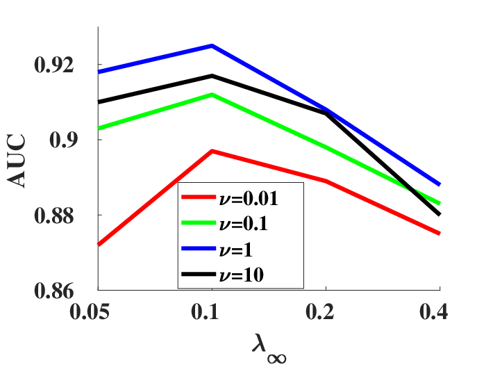
Figures 3 and 4 show the results of the deep learning implementation of BSPAUC with different hyper-parameter values. Figure 3 clearly reveals that with the increase of $\lambda_{\infty}$ , AUC increases first and then decreases gradually. This phenomenon is expected. When $\lambda_{\infty}$ is small, increasing $\lambda_{\infty}$ will cause more easy samples to join the training and thus the generalization of model is improved. However, when $\lambda_{\infty}$ is large enough, complex (noise) samples start being included and then AUC decreases. What’s more, Figure 4 directly reflects that with the increase of $\mu$ , which can be calculated by $\mu=\nu\lambda_{\infty}$ , the proportions of selected positive and negative samples gradually approach. Further more, combining with the above two figures, we observe that too large APD often tends to low AUC. Large APD often implies that some easy samples in the class with low proportion of selected samples don’t join the training while some complex samples in the other class with high proportion are selected. The above case leads to the reduction of generalization ability and thus causes low AUC. Importantly, our balanced self-paced regularization term is proposed for this issue.

Conclusion

In this paper, we first provide a statistical explanation to self-paced AUC. Inspired by this, we propose our self-paced AUC maximization formulation with a novel balanced self-paced regularization term. Then we propose a doubly cyclic block coordinate descent algorithm (i.e., BSPAUC) to optimize our objective function. Importantly, we prove that the sub-problem with respect to all weight variables converges to a stationary point on the basis of closed-form solutions, and our BSPAUC converges to a stationary point of our fixed optimization objective under a mild assumption. The experimental results demonstrate that our BSPAUC outperforms existing state-of-the-art AUC maximization methods and has better robustness.

Acknowledgments

Bin Gu was partially supported by the National Natural Science Foundation of China (No:61573191).

Appendix A. Table 3 with standard deviation

Mean AUC results with the corresponding standard deviation on noisy datasets are shown in Table 3. The results clearly show that our BSPAUC achieves the best performance on all noisy datasets. Specifically, the larger the proportion of noisy data is, the more obvious the advantage is. Our BSPAUC excludes the noise samples from training by giving a zero weight and thus has a better robustness.

Table 3: Mean AUC results with the corresponding standard deviation on noisy datasets. (FP means the proportion of noise samples constructed by flipping labels, PP denotes the proportion of injected poison samples and ’–’ means out of memory.)

Datasets	rcv1			a9a
FP	$10\%$	$20\%$	$30\%$	$10\%$	$20\%$	$30\%$
OPAUC	0.958 $\pm$ 0.015	0.933 $\pm$ 0.025	0.845 $\pm$ 0.023	0.824 $\pm$ 0.009	0.804 $\pm$ 0.013	0.778 $\pm$ 0.016
KOIL_FIFO++	0.901 $\pm$ 0.026	0.889 $\pm$ 0.031	0.804 $\pm$ 0.042	0.836 $\pm$ 0.015	0.806 $\pm$ 0.024	0.726 $\pm$ 0.033
TSAM	0.961 $\pm$ 0.002	0.946 $\pm$ 0.015	0.838 $\pm$ 0.024	0.877 $\pm$ 0.012	0.846 $\pm$ 0.015	0.752 $\pm$ 0.018
PDD_SG	0.964 $\pm$ 0.002	0.936 $\pm$ 0.007	0.855 $\pm$ 0.017	0.881 $\pm$ 0.002	0.849 $\pm$ 0.002	0.739 $\pm$ 0.006
DSAM	0.983 $\pm$ 0.005	0.962 $\pm$ 0.011	0.862 $\pm$ 0.034	0.886 $\pm$ 0.003	0.837 $\pm$ 0.007	0.811 $\pm$ 0.006
BSPAUC	0.991 $\pm$ 0.002	0.985 $\pm$ 0.009	0.945 $\pm$ 0.009	0.914 $\pm$ 0.006	0.894 $\pm$ 0.012	0.883 $\pm$ 0.010
Datasets	skin_nonskin			cod-rna
FP	$10\%$	$20\%$	$30\%$	$10\%$	$20\%$	$30\%$
OPAUC	0.925 $\pm$ 0.009	0.884 $\pm$ 0.009	0.815 $\pm$ 0.008	0.902 $\pm$ 0.021	0.864 $\pm$ 0.036	0.783 $\pm$ 0.034
KOIL_FIFO++	—	—	—	—	—	—
TSAM	0.937 $\pm$ 0.001	0.913 $\pm$ 0.004	0.842 $\pm$ 0.007	0.933 $\pm$ 0.006	0.880 $\pm$ 0.004	0.808 $\pm$ 0.015
PDD_SG	0.940 $\pm$ 0.001	0.912 $\pm$ 0.004	0.852 $\pm$ 0.012	0.937 $\pm$ 0.002	0.873 $\pm$ 0.006	0.788 $\pm$ 0.021
DSAM	0.961 $\pm$ 0.003	0.917 $\pm$ 0.002	0.819 $\pm$ 0.014	0.975 $\pm$ 0.002	0.922 $\pm$ 0.002	0.781 $\pm$ 0.016
BSPAUC	0.979 $\pm$ 0.001	0.944 $\pm$ 0.002	0.912 $\pm$ 0.010	0.990 $\pm$ 0.001	0.956 $\pm$ 0.001	0.874 $\pm$ 0.007
Datasets	rcv1			a9a
PP	$10\%$	$20\%$	$30\%$	$10\%$	$20\%$	$30\%$
OPAUC	0.923 $\pm$ 0.016	0.863 $\pm$ 0.020	0.803 $\pm$ 0.026	0.833 $\pm$ 0.015	0.816 $\pm$ 0.018	0.797 $\pm$ 0.016
KOIL_FIFO++	0.891 $\pm$ 0.023	0.838 $\pm$ 0.027	0.793 $\pm$ 0.044	0.831 $\pm$ 0.022	0.823 $\pm$ 0.034	0.806 $\pm$ 0.035
TSAM	0.930 $\pm$ 0.002	0.859 $\pm$ 0.012	0.809 $\pm$ 0.021	0.872 $\pm$ 0.002	0.849 $\pm$ 0.002	0.838 $\pm$ 0.005
PDD_SG	0.934 $\pm$ 0.003	0.918 $\pm$ 0.005	0.828 $\pm$ 0.017	0.885 $\pm$ 0.002	0.873 $\pm$ 0.001	0.839 $\pm$ 0.004
DSAM	0.902 $\pm$ 0.007	0.845 $\pm$ 0.017	0.757 $\pm$ 0.051	0.881 $\pm$ 0.004	0.852 $\pm$ 0.004	0.843 $\pm$ 0.009
BSPAUC	0.955 $\pm$ 0.002	0.937 $\pm$ 0.003	0.876 $\pm$ 0.010	0.911 $\pm$ 0.002	0.907 $\pm$ 0.002	0.896 $\pm$ 0.008
Datasets	skin_nonskin			cod-rna
PP	$10\%$	$20\%$	$30\%$	$10\%$	$20\%$	$30\%$
OPAUC	0.927 $\pm$ 0.010	0.880 $\pm$ 0.020	0.856 $\pm$ 0.021	0.914 $\pm$ 0.015	0.893 $\pm$ 0.023	0.858 $\pm$ 0.034
KOIL_FIFO++	—	—	—	—	—	—
TSAM	0.933 $\pm$ 0.002	0.911 $\pm$ 0.004	0.877 $\pm$ 0.005	0.953 $\pm$ 0.002	0.903 $\pm$ 0.006	0.886 $\pm$ 0.005
PDD_SG	0.935 $\pm$ 0.001	0.927 $\pm$ 0.002	0.898 $\pm$ 0.009	0.972 $\pm$ 0.001	0.941 $\pm$ 0.001	0.881 $\pm$ 0.014
DSAM	0.980 $\pm$ 0.001	0.954 $\pm$ 0.001	0.902 $\pm$ 0.005	0.973 $\pm$ 0.004	0.938 $\pm$ 0.005	0.913 $\pm$ 0.004
BSPAUC	0.995 $\pm$ 0.001	0.982 $\pm$ 0.001	0.965 $\pm$ 0.006	0.991 $\pm$ 0.003	0.973 $\pm$ 0.003	0.953 $\pm$ 0.008

Appendix B. Implementation of Algorithm 3

When we fix $\mathbf{v},\mathbf{u}$ to update $\theta$ :

\theta^{t}=\argmin\limits_{\theta}\frac{1}{nm}\sum_{i=1}^{n}\sum_{j=1}^{m}v_{i}u_{j}\xi_{ij}+\tau\Omega(\theta)+\text{const},

(13)

where $\xi_{ij}=\max\{1-f(x^{+}_{i})+f(x^{-}_{j}),0\}$ .

For the kernel-based implementation of solving Eq. (13), we also compute the gradient on random pairs of weighted samples which are selected from two subsets $\hat{X}^{+}$ and $\hat{X}^{-}$ respectively. In this case, the weighted batch AUC loss is defined as:

\displaystyle\sum_{j=1}^{\pi}v_{j}u_{j}\xi_{jj}=\sum_{j=1}^{\pi}v_{j}u_{j}\max\{1-f(x^{+}_{j})+f(x^{-}_{j}),0\}.

(14)

Then, we apply random Fourier feature method to approximate the kernel function (Rahimi and Recht 2008; Dai et al. 2014) for large-scale problems. The mapping function of $D$ random features is defined as

	$\displaystyle\phi_{\omega}(x)=\sqrt{1/D}[$	$\displaystyle\cos(\omega_{1}x),\ldots,\cos(\omega_{D}x),$
		$\displaystyle\sin(\omega_{1}x),\ldots,\sin(\omega_{D}x)]^{T},$

where $\omega_{i}$ is randomly sampled according to the density function $p(\omega)$ associated with $k(x,x^{\prime})$ (Odland 2017). Then, based on the weighted batch AUC loss (14) and the random feature mapping function $\phi_{\omega}(x)$ , we obtain Algorithm 3 by applying the triply stochastic gradient descent method (TSGD) (Dang et al. 2020) w.r.t. random pairs of weighted samples and random features.

Algorithm 3 Kernel-based implementation of solving Eq. (13)

p(\omega),\phi_{\omega}(x),\tau,T,\mathbf{\eta},\hat{X}^{+},\hat{X}^{-},\pi,\theta^{0}

1: for

i=1,\cdots,T

2: Sample

\hat{x}^{+}_{1},...,\hat{x}^{+}_{\pi}

from

\hat{X}^{+}

3: Sample

\hat{x}^{-}_{1},...,\hat{x}^{-}_{\pi}

from

\hat{X}^{-}

4: Sample

\omega_{i}

\sim

p(\omega)

with seed

i

5: Calculate

f({x})

by Predict

(x,\{\alpha_{i}\}_{j=1}^{i-1})

6: Get

\alpha_{i}

according to the following formula:

\displaystyle\alpha_{i}=

\displaystyle-\frac{\eta_{i}}{\pi}\sum_{j=1}^{\pi}v_{j}u_{j}\frac{\partial\xi_{jj}}{\partial\theta}.\qquad\qquad\qquad\qquad

7: Update

\alpha_{j}=(1-\eta_{j}\tau)\alpha_{j},j\in[1,i-1]

8: end for

\theta=\{\alpha_{i}\}_{i=1}^{T}

Algorithm 4

f(x)=

Predict

(x,\{\alpha_{i}\}_{i=1}^{t})

p(\omega),\phi_{\omega}(x),x,\{\alpha_{i}\}_{i=1}^{t}

1: Set

f(x)=0

2: for

i=1,\cdots,t

3: Sample

\omega_{i}

\sim

p(\omega)

with seed

i

f(x)=f(x)+\alpha_{i}\phi_{\omega_{i}}(x)

5: end for

f(x)

Appendix C. Proof of Theorem 1

Firstly, we introduce some notions again. Let $X$ be a compact subset of $\mathbb{R}^{d}$ , $Y=\{-1,+1\}$ be the label set and $Z=X\times Y$ . Given a distribution $P(z)$ and let $S=\{z_{i}=(x_{i},y_{i})\}_{i=1}^{n}$ be an independent and identically distributed (IID) training set drawn from $P(z)$ , where $x_{i}\in X$ , $y_{i}\in Y$ and $z_{i}\in Z$ . Thus, empirical AUC risk on $S$ can be formulated as:

\displaystyle R_{emp}(S;f)=\frac{1}{n(n-1)}\sum_{z_{i},z_{j}\in S,z_{i}\neq z_{j}}L_{f}(z_{i},z_{j}).

(15)

Here, $f\in\mathcal{F}:\mathbb{R}^{d}\to\mathbb{R}$ is one real-valued function and the pairwise loss function $L_{f}(z_{i},z_{j})$ for AUC is defined as:

L_{f}(z_{i},z_{j})=\left\{\begin{array}[]{l@{\ \ \textrm{if} \ \ }l}0&\ y_{i}=y_{j}\\ \mathbb{I}(f(x_{i})\leq f(x_{j}))&y_{i}=+1\&\ y_{j}=-1\\ \mathbb{I}(f(x_{j})\leq f(x_{i}))&y_{j}=+1\&\ y_{i}=-1\end{array}\right.

where $\mathbb{I}(\cdot)$ is the indicator function such that $\mathbb{I}(\pi)$ equals 1 if $\pi$ is true and 0 otherwise.

Further, the expected risk of AUC for the distribution $P(z)$ can be defined as:

	$\displaystyle R_{exp}(P(z);f):=\mathbb{E}_{z_{1},z_{2}\sim P(z)^{2}}L_{f}(z_{1},z_{2})$
$\displaystyle=$	$\displaystyle\mathbb{E}_{S\sim P(z)^{n}}\left[\frac{1}{n(n-1)}\sum_{z_{i},z_{j}\in S,z_{i}\neq z_{j}}L_{f}(z_{i},z_{j})\right]$
$\displaystyle=$	$\displaystyle\mathbb{E}_{S}[R_{emp}(S;f)].$	(16)

Under the assumption that our training set in reality is composed by not only target clean data but also a proportion of noise samples, Gong et al. (Gong et al. 2016) connect the data distribution $P_{train}(z)$ of the training set with the distribution $P_{target}(z)$ of the target set using a weight function $W_{\lambda}(z)$ :

		$\displaystyle P_{target}(z)=\frac{1}{\alpha_{*}}W_{\lambda}(z)P_{train}(z),$		(17)
		$\displaystyle\alpha_{*}=\int_{Z}W_{\lambda}(z)P_{train}(z)dz,$

where $0\leq W_{\lambda}(z)\leq 1$ and $\alpha_{*}$ denotes the normalization factor. Intuitively, $W_{\lambda}(z)$ gives larger weights to easy samples than to complex samples and with the increase of pace parameter $\lambda$ , all samples tend to be assigned larger weights.

Then, Eq. (17) can be reformulated as:

		$\displaystyle P_{train}(z)=\alpha_{}P_{target}(z)+(1-\alpha_{})E(z),$		(18)
		$\displaystyle E(z)=\frac{1}{1-\alpha_{}}(1-W_{\lambda_{}}(z))P_{train}(z).$

Based on (18), we define the pace distribution $Q_{\lambda}(z)$ as:

\displaystyle Q_{\lambda}(z)=\alpha_{\lambda}P_{target}(z)+(1-\alpha_{\lambda})E(z),

(19)

\displaystyle Q_{\lambda}(z)\propto W_{\lambda}(z)P_{train}(z).

(20)

Here,

\displaystyle W_{\lambda}(z)\propto\frac{\alpha_{\lambda}P_{target}(z)+(1-\alpha_{\lambda})E(z)}{\alpha_{*}P_{target}(z)+(1-\alpha_{*})E(z)},

and

		$\displaystyle\frac{\alpha_{\lambda}P_{target}(z)+(1-\alpha_{\lambda})E(z)}{\alpha_{}P_{target}(z)+(1-\alpha_{})E(z)}$
	$\displaystyle=$	$\displaystyle\frac{\alpha_{\lambda}P_{target}(z)+(1-\alpha_{\lambda})E(z)}{P_{train}(z)},$

where $0\leq W_{\lambda}(z)\leq 1$ through normalizing its maximal value to 1.

Then, after introducing the definition of McDiarmid inequality, we obtain the relationship between the empirical AUC risk $R_{emp}$ (15) and the expected AUC risk $R_{exp}$ (Appendix C. Proof of Theorem ) in Lemma 1.

Definition 1.

(McDiarmid Inequality) Let $z_{1},...z_{n}\in S$ be a set of independent random variables and assume that there exists $c_{1},...,c_{n}>0$ such that $f:S^{n}\rightarrow\mathbb{R}$ satisfies the following inequalities:

\displaystyle|f(z_{1},...,z_{i},...,z_{n})-f(z_{1},...,z_{i}^{\prime},...z_{n})|\leq c_{i},

for all $i\in\{1,...,n\}$ and points $z_{1}^{\prime},...z_{n}^{\prime}\in S$ . Then, $\forall\epsilon>0$ we have

		$\displaystyle P(f(z_{1},...,z_{n})-\mathbb{E}(f(z_{1},...,z_{n}))\geq\epsilon)\leq\exp\left(\frac{-2\epsilon^{2}}{\sum_{i=1}^{n}c_{i}^{2}}\right)$
		$\displaystyle P(f(z_{1},...,z_{n})-\mathbb{E}(f(z_{1},...,z_{n}))\leq-\epsilon)\leq\exp\left(\frac{-2\epsilon^{2}}{\sum_{i=1}^{n}c_{i}^{2}}\right)$

Lemma 1.

An independent and identically distributed sample set $S=\{z_{1},...,z_{n}\},z_{i}\in Z$ is obtained according to the distribution $P(z)$ . Then for any $\delta>0$ and any $f\in\mathcal{F}$ , the following holds for $R_{emp}$ (15) and $R_{exp}$ (Appendix C. Proof of Theorem ) with confidence at least $1-\delta$ :

\displaystyle R_{exp}(P(z);f)\leq R_{emp}(S;f)+\sqrt{\frac{\ln(1/\delta)}{n/2}}.

(21)

Proof.

Let $S^{\prime}$ be a set of samples same as $S$ and then we change the $z\in S^{\prime}$ to $z^{\prime}$ . In this case, $S^{\prime}$ is different from $S$ with only one sample and $z\in S,z^{\prime}\in S^{\prime}$ are the two different samples. Then, we have

		$\displaystyle R_{emp}(S;f)-R_{emp}(S^{\prime};f)$
	$\displaystyle\overset{a}{=}$	$\displaystyle\frac{2}{n(n-1)}\left(\sum_{z_{j}\in S,z_{j}\neq z}L_{f}(z,z_{j})-\sum_{z_{j}\in S^{\prime},z_{j}\neq z^{\prime}}L_{f}(z^{\prime},z_{j})\right)$
	$\displaystyle\overset{b}{\leq}$	$\displaystyle\frac{2(n-1)}{n(n-1)}=\frac{2}{n}$

The equality (a) is due to the property that $\forall z_{i},z_{j}\in Z,L_{f}(z_{i},z_{j})=L_{f}(z_{j},z_{i})$ , and the inequality (b) is obtained by the fact that the function $L_{f}$ is bounded by $[0,1]$ . Similarly, we can get

\displaystyle|R_{emp}(S;f)-R_{emp}(S^{\prime};f)|\leq\frac{2}{n}.

According to Definition 1, $\forall\epsilon>0$ we have

		$\displaystyle P(R_{emp}(S;f)-E_{S}[R_{emp}(S;f)]\leq-\epsilon)\leq\exp(\frac{-\epsilon^{2}}{2/n})$
	$\displaystyle\iff$	$\displaystyle P(R_{emp}(S;f)-R_{exp}(P(z);f)\geq-\epsilon)\geq 1-\exp(\frac{-\epsilon^{2}}{2/n})$

Then, we define $\delta$ as $\exp(\frac{-\epsilon^{2}}{2/n})$ and calculate $\epsilon$ as $\sqrt{\frac{\ln(1/\delta)}{n/2}}$ .
In this case, we proof that with confidence at least $1-\delta$ , the following holds

\displaystyle R_{exp}(P(z);f)\leq R_{emp}(S;f)+\sqrt{\frac{\ln(1/\delta)}{n/2}}.

(22)

The proof is then completed. ∎

Combining with the pace distribution $Q_{\lambda}$ (19), we get the following Lemma.

Lemma 2.

An independent and identically distributed sample set $S=\{z_{1},...,z_{n}\}$ is obtained according to the pace distribution $Q_{\lambda}$ (19). Then for any $\delta>0$ and any $f\in\mathcal{F}$ , with confidence at least $1-\delta$ we have:

\displaystyle R_{exp}(P_{target};f)

\displaystyle\leq R_{emp}(S;f)+e_{\lambda}+\sqrt{\frac{\ln(1/\delta)}{n/2}}

(23)

where $e_{\lambda}$ is defined as $R_{exp}(P_{target};f)-R_{exp}(Q_{\lambda};f)$ and with the increasing of $\lambda$ , $e_{\lambda}$ decreases monotonically from $0$ .

Proof.

The empirical risk in training set tends not to approximate the expected risk due to the inconsistence of $P_{train}$ and $P_{target}$ . However, by introducing pace empirical risk with pace distribution $Q_{\lambda}$ in the error analysis, we can formulate the following error decomposition:

		$\displaystyle R_{exp}(P_{target};f)-R_{emp}(S;f)$		(24)
	$\displaystyle=$	$\displaystyle R_{exp}(P_{target};f)-R_{exp}(Q_{\lambda};f)+R_{exp}(Q_{\lambda};f)-R_{emp}(S;f),$

and we define

\displaystyle e_{\lambda}=R_{exp}(P_{target};f)-R_{exp}(Q_{\lambda};f).

(25)

Considering the definition of $Q_{\lambda}$ (19) which simulates the changing process from $P_{target}$ to $P_{train}$ and the relationship (17) between $P_{train}$ and $P_{target}$ , we conclude that with the increasing of $\lambda$ , $e_{\lambda}$ decreases monotonically from $0$ .
Because $S$ is subject to the pace distribution $Q_{\lambda}$ (19), according to Lemma 1, the following holds with confidence $1-\delta$

\displaystyle R_{exp}(Q_{\lambda};f)-R_{emp}(S;f)\leq\sqrt{\frac{\ln(1/\delta)}{n/2}}.

(26)

Combining (24),(25) with (26), we have

\displaystyle R_{exp}(P_{target};f)\leq R_{emp}(S;f)+e_{\lambda}+\sqrt{\frac{\ln(1/\delta)}{n/2}}.

The proof is then completed. ∎

Finally, the proof of Theorem 1 is as follows.

Proof.

When we use training set $S=\{z_{1},...,z_{m}\}$ to approximate $P_{train}$ , we have

\displaystyle P_{train}=\sum_{i=1}^{m}p_{i}D_{z_{i}}(z),\ \forall i\in\{1,...,m\},

where $p_{i}=\frac{1}{m}$ and $D_{z_{i}}(z)$ denotes the Dirac delta function centered at $z_{i}$ :

\displaystyle\forall z!=z_{i},\ D_{z_{i}}(z)=0\ \text{and}\ \int_{Z}D_{z_{i}}(z)dz=1.

It is easy to see that $P_{train}$ supposes a uniform density on each sample $z_{i}$ . Next, according to the special formulation (20) of $Q_{\lambda}$ , we have:

\displaystyle Q_{\lambda}(z)\propto\sum_{i=1}^{m}W_{\lambda}(z_{i})p_{i}D_{z_{i}}(z).

In this case, $S_{Q}=\{W_{\lambda}(z_{1})z_{1},...,W_{\lambda}(z_{m})z_{m}\}$ is subject to the pace distribution $Q_{\lambda}$ . And the empirical risk on $Q_{\lambda}$ can be rewritten as

		$\displaystyle R_{emp}(S_{Q};f)$
	$\displaystyle=$	$\displaystyle\frac{1}{n_{\lambda}(n_{\lambda}-1)}\sum_{z_{i},z_{j}\in S,z_{i}\neq z_{j}}W_{\lambda}(z_{i})W_{\lambda}(z_{j})L_{f}(z_{i},z_{j})$

where $n_{\lambda}=\sum_{i=1}^{m}\mathbb{I}(W_{\lambda}(z_{i})!=0)$ denotes the number of selected samples in SPL setting.

And combining with Lemma 2, we conclude that for any $\delta>0$ and any $f\in\mathcal{F}$ , with confidence at least $1-\delta$ over a sample set $S$ , we have:

	$\displaystyle R_{exp}(P_{target};f)\leq$	$\displaystyle\frac{1}{n_{\lambda}(n_{\lambda}-1)}\sum_{z_{i},z_{j}\in S\atop z_{i}\neq z_{j}}W_{\lambda}(z_{i})W_{\lambda}(z_{j})L_{f}(z_{i},z_{j})$
	$\displaystyle+$	$\displaystyle e_{\lambda}+\sqrt{\frac{\ln(1/\delta)}{n_{\lambda}/2}},$		(27)

where $n_{\lambda}$ denotes the number of selected samples, $e_{\lambda}$ is defined as $R_{exp}(P_{target};f)-R_{exp}(Q_{\lambda};f)$ and with the increasing of $\lambda$ , $e_{\lambda}$ decreases monotonically from $0$ . ∎

Appendix D. Proof of Theorem 2

The objective function of our BSPAUC is defined as follows:

	$\displaystyle\min_{\theta,\mathbf{v},\mathbf{u}}\ \mathcal{L}(\theta,\mathbf{v},\mathbf{u};\lambda)$	(28)
$\displaystyle=$	$\displaystyle\min_{\theta,\mathbf{v},\mathbf{u}}\ \frac{1}{nm}\sum_{i=1}^{n}\sum_{j=1}^{m}v_{i}u_{j}\xi_{ij}+\tau\Omega(\theta)$	(29)
$\displaystyle-$	$\displaystyle\lambda\left(\frac{1}{n}\sum_{i=1}^{n}v_{i}+\frac{1}{m}\sum_{j=1}^{m}u_{j}\right)+\mu\left(\frac{1}{n}\sum_{i=1}^{n}v_{i}-\frac{1}{m}\sum_{j=1}^{m}u_{j}\right)^{2}$
	$\displaystyle\ s.t.\ \mathbf{v}\in[0,1]^{n},\mathbf{u}\in[0,1]^{m}$

where $\xi_{ij}=\max\{1-f(x^{+}_{i})+f(x^{-}_{j}),0\}$ is the pairwise hinge loss.

Proof.

For the sake of clarity, we define $\mathcal{K}(\mathbf{v},\mathbf{u})=\mathcal{L}(\mathbf{v},\mathbf{u};\theta,\lambda)$ as the sub-problem of (28) where $\theta$ and $\lambda$ are fixed:

	$\displaystyle\min_{\mathbf{v},\mathbf{u}}\ \mathcal{K}(\mathbf{v},\mathbf{u})=\min_{\mathbf{v},\mathbf{u}}\ \mathcal{L}(\mathbf{v},\mathbf{u};\theta,\lambda)$	(30)
$\displaystyle=$	$\displaystyle\min_{\mathbf{v},\mathbf{u}}\ \frac{1}{nm}\sum_{i=1}^{n}\sum_{j=1}^{m}v_{i}u_{j}\xi_{ij}-\lambda\left(\frac{1}{n}\sum_{i=1}^{n}v_{i}+\frac{1}{m}\sum_{j=1}^{m}u_{j}\right)$
$\displaystyle+$	$\displaystyle\mu\left(\frac{1}{n}\sum_{i=1}^{n}v_{i}-\frac{1}{m}\sum_{j=1}^{m}u_{j}\right)^{2}+\text{const}$
	$\displaystyle\ s.t.\ \mathbf{v}\in[0,1]^{n},\mathbf{u}\in[0,1]^{m}$

First of all, we have to be clear that the necessary condition for $\mathcal{K}(\mathbf{v},\mathbf{u})$ to be a convex function is

		$\displaystyle\mathcal{K}(\frac{1}{2}(\mathbf{v}^{1}+\mathbf{v}^{2}),\frac{1}{2}(\mathbf{u}^{1}+\mathbf{u}^{2}))-\frac{1}{2}(\mathcal{K}(\mathbf{v}^{1},\mathbf{u}^{1})+\mathcal{K}(\mathbf{v}^{2},\mathbf{u}^{2}))\leq 0,$		(31)
		$\displaystyle\mathbf{v}^{1},\mathbf{v}^{2}\in[0,1]^{n},\mathbf{u}^{1},\mathbf{u}^{2}\in[0,1]^{m}.$		(31)

Without loss of generality, let

	$\displaystyle\mathbf{v}^{1}=(1,1,...,1),\mathbf{u}^{1}=(0,0,...,0),$
	$\displaystyle\mathbf{v}^{2}=(0,0,...,0),\mathbf{u}^{2}=(1,1,...,1).$

Then $\mathcal{K}(\mathbf{v},\mathbf{u})$ satisfies

		$\displaystyle\mathcal{K}(\frac{1}{2}(\mathbf{v}^{1}+\mathbf{v}^{2}),\frac{1}{2}(\mathbf{u}^{1}+\mathbf{u}^{2}))-\frac{1}{2}(\mathcal{K}(\mathbf{v}^{1},\mathbf{u}^{1})+\mathcal{K}(\mathbf{v}^{2},\mathbf{u}^{2}))$
	$\displaystyle=$	$\displaystyle\frac{1}{4nm}\sum_{i=1}^{n}\sum_{j=1}^{m}\xi_{ij}-\mu.$

Due to the condition that $\mu$ is a hyperparameter greater than 0 and $\xi_{ij}$ is not less than 0, the formula $\frac{1}{4nm}\sum_{i=1}^{n}\sum_{j=1}^{m}\xi_{ij}-\mu$ is not guaranteed to be less than or equal to 0. And then according to the necessary condition (31), we can conclude that if we fix $\theta$ in Eq. (28), the sub-problem with respect to $\mathbf{v}$ and $\mathbf{u}$ maybe non-convex. ∎

Appendix E. Proof of Theorem 3

When we fix $\mathbf{u}$ and $\theta$ , the sub-problem with respect to $\mathbf{v}$ is as follows:

	$\displaystyle\mathbf{v}^{t}=$	$\displaystyle\argmin\limits_{\mathbf{v}\in[0,1]^{n}}\ \mathcal{L}(\mathbf{v};\theta,\mathbf{u},\lambda)$		(32)
	$\displaystyle=$	$\displaystyle\argmin\limits_{\mathbf{v}\in[0,1]^{n}}\ \frac{1}{n}\sum_{i=1}^{n}v_{i}l^{+}_{i}-\lambda\frac{1}{n}\sum_{i=1}^{n}v_{i}+\mu\left(\frac{1}{n}\sum_{i=1}^{n}v_{i}-Q\right)^{2}+\text{const},$

where $l^{+}_{i}=\frac{1}{m}\sum_{j=1}^{m}u_{j}\xi_{ij}$ and $Q=\frac{1}{m}\sum_{j=1}^{m}u_{j}$ .

And when we fix $\mathbf{v}$ and $\theta$ , the sub-problem with respect to $\mathbf{u}$ is as follows:

	$\displaystyle\mathbf{u}^{t}=$	$\displaystyle\argmin\limits_{\mathbf{u}\in[0,1]^{m}}\ \mathcal{L}(\mathbf{u};\theta,\mathbf{v},\lambda)$		(33)
	$\displaystyle=$	$\displaystyle\argmin\limits_{\mathbf{u}\in[0,1]^{m}}\ \frac{1}{m}\sum_{j=1}^{m}u_{j}l^{-}_{j}-\lambda\frac{1}{m}\sum_{j=1}^{m}u_{j}+\mu\left(\frac{1}{m}\sum_{j=1}^{m}u_{j}-P\right)^{2}+\text{const},$

where $l^{-}_{j}=\frac{1}{n}\sum_{i=1}^{n}v_{i}\xi_{ij}$ and $P=\frac{1}{n}\sum_{i=1}^{n}v_{i}$ .

Proof.

Eq. (32) can be expressed as

	$\displaystyle\argmin\limits_{\mathbf{v}\in[0,1]^{n}}\quad\frac{1}{n}\sum_{i=1}^{n}v_{i}l^{+}_{i}-\lambda\frac{1}{n}\sum_{i=1}^{n}v_{i}+\mu(\frac{1}{n}\sum_{i=1}^{n}v_{i}-Q)^{2}$
$\displaystyle\iff$	$\displaystyle\argmin\limits_{\mathbf{v}\in[0,1]^{n}}\quad\sum_{i=1}^{n}v_{i}b_{i}+\frac{1}{n}(\sum_{i=1}^{n}v_{i}-nQ)^{2}$	(34)
$\displaystyle:=$	$\displaystyle\argmin\limits_{\mathbf{v}\in[0,1]^{n}}\quad F(\mathbf{v})$	(35)

where $l^{+}_{i}=\frac{1}{m}\sum_{j=1}^{m}u_{j}\xi_{ij}$ , $Q=\frac{1}{m}\sum_{j=1}^{m}u_{j}$ and $b_{i}=\frac{l_{i}^{+}-\lambda}{\mu}$ .
Without loss of generality, we suppose that $b_{1}\leq b_{2}\leq\cdots\leq b_{n}$ . In this case, we firstly proof that the following $\mathbf{v}=(1,1,\ldots,1,v_{p},0,0,\ldots,0)$ , which means that the $p$ -th element $v_{p}$ is the only element in $\mathbf{v}$ that can not equal to 0 or 1, minimizes $F(\mathbf{v})$ .
For each $\mathbf{v}\in[0,1]^{n}$ , if $v_{i}<v_{j}$ for some $i<j$ , then we can exchange $v_{i}$ and $v_{j}$ , thus $\mathbf{v}$ becomes $\mathbf{v^{\prime}}$ . We have

		$\displaystyle F(\mathbf{v^{\prime}})-F(\mathbf{v})$
	$\displaystyle=$	$\displaystyle(b_{i}v_{j}+b_{j}v_{i})-(b_{i}v_{i}+b_{j}v_{j})=(b_{i}-b_{j})(v_{j}-v_{i})\leq 0.$

Therefore, we can always assume that $1\geq v_{1}\geq v_{2}\geq\cdots\geq v_{n}\geq 0$ when $\mathbf{v}$ minimizes $F(\mathbf{v})$ .
Assuming that there exist $1>v_{i}>v_{i+1}>0$ , we consider the following two cases.
Case 1: $v_{i}+v_{i+1}\geq 1$ . In this case, we replace $(v_{i},v_{i+1})$ by $(1,v_{i}+v_{i+1}-1)$ , then $\mathbf{v}$ becomes $\mathbf{v^{\prime}}$ . And we have

		$\displaystyle F(\mathbf{v^{\prime}})-F(\mathbf{v})$
	$\displaystyle=$	$\displaystyle(b_{i}+b_{i+1}(v_{i}+v_{i+1}-1))-(b_{i}v_{i}+b_{i+1}v_{i+1})$
	$\displaystyle=$	$\displaystyle(b_{i}-b_{i+1})(1-v_{i})\leq 0.$

Case 2: $v_{i}+v_{i+1}<1$ . In this case, we replace $(v_{i},v_{i+1})$ by $(v_{i}+v_{i+1},0)$ , then $\mathbf{v}$ becomes $\mathbf{v^{\prime}}$ . And we have

	$\displaystyle F(\mathbf{v^{\prime}})-F(\mathbf{v})$	$\displaystyle=b_{i}(v_{i}+v_{i+1})-(b_{i}v_{i}+b_{i+1}v_{i+1})$
		$\displaystyle=(b_{i}-b_{i+1})v_{i+1}\leq 0.$

Therefore, we can always assume that at most one element in $\mathbf{v}$ is not equal to 0 or 1 when $\mathbf{v}$ minimizes $F(\mathbf{v})$ .
According to the fact that $1\geq v_{1}\geq v_{2}\geq\cdots\geq v_{n}\geq 0$ and at most one element in $\mathbf{v}$ is not equal to 0 or 1 when $\mathbf{v}$ minimizes $F(\mathbf{v})$ , we conclude that the following $\mathbf{v}=(1,1,\ldots,1,v_{p},0,0,\ldots,0)$ , which means that the $p$ -th element $v_{p}$ is the only element in $\mathbf{v}$ that can not equal to 0 or 1, minimizes $F(\mathbf{v})$ .
Then, we rewrite $F(\mathbf{v})$ as

\displaystyle F(\mathbf{v})=\frac{1}{n}(v_{p}+p-1+\frac{nb_{p}}{2}-nQ)^{2}+\text{const}

(36)

and consider the following three cases when $\mathbf{v}=(1,1,\ldots,1,v_{p},0,0,\ldots,0)$ minimizes $F(\mathbf{v})$ .
Case 1: $v_{p}=1$ . According to Eq. (36) we have that

p-1+\frac{nb_{p}}{2}-nQ\leq-1

and thus

-\frac{b_{p}}{2}\geq\frac{p}{n}-Q.

Furthermore, for each $i<p$ we have $v_{i}=1$ and

-\frac{b_{i}}{2}\geq-\frac{b_{p}}{2}\geq\frac{p}{n}-Q\geq\frac{i}{n}-Q.

And for each $i>p$ we have $v_{i}=0$ , we rewrite $F(\mathbf{v})$ as

F(\mathbf{v})=\frac{1}{n}(v_{i}+p+\frac{nb_{i}}{2}-nQ)^{2}+\text{const}.

Since $\mathbf{v}$ minimizes $F(\mathbf{v})$ , we have

p+\frac{nb_{i}}{2}-nQ\geq 0

and thus

-\frac{b_{i}}{2}\leq\frac{p}{n}-Q\leq\frac{i-1}{n}-Q.

Therefore, in this case we can get $\forall i\in\{1,2,...,n\}$ ,

	$\displaystyle v_{i}=1$	$\displaystyle\iff-\frac{b_{i}}{2}\geq\frac{i}{n}-Q,$		(37)
	$\displaystyle v_{i}=0$	$\displaystyle\iff-\frac{b_{i}}{2}\leq\frac{i-1}{n}-Q.$		(38)

Case 2: $0<v_{p}<1$ . According to Eq. (36) we have that

0<v_{p}=-(p-1+\frac{nb_{p}}{2}-nQ)<1

and thus

\frac{p-1}{n}-Q<-\frac{b_{p}}{2}<\frac{p}{n}-Q.

Furthermore, for each $i<p$ we have $v_{i}=1$ , we rewrite $F(\mathbf{v})$ as

F(\mathbf{v})=\frac{1}{n}(v_{i}+p-2+v_{p}+\frac{nb_{i}}{2}-nQ)^{2}+\text{const}.

Since $\mathbf{v}$ minimizes $F(\mathbf{v})$ , we have

p-2+v_{p}+\frac{nb_{i}}{2}-nQ\leq-1

and thus

-\frac{b_{i}}{2}\geq\frac{p-1+v_{p}}{n}-Q\geq\frac{i}{n}-Q.

And for each $i>p$ we have $v_{i}=0$ , we rewrite $F(\mathbf{v})$ as

F(\mathbf{v})=\frac{1}{n}(v_{i}+p-1+v_{p}+\frac{nb_{i}}{2}-nQ)^{2}+\text{const}.

Since $\mathbf{v}$ minimizes $F(\mathbf{v})$ , we have

p-1+v_{p}+\frac{nb_{i}}{2}-nQ\geq 0

and thus

-\frac{b_{i}}{2}\leq\frac{p-1+v_{p}}{n}-Q\leq\frac{i-1}{n}-Q.

Therefore, in this case we can get $\forall i\in\{1,2,...,n\}$ ,

		$\displaystyle v_{i}=1\iff-\frac{b_{i}}{2}\geq\frac{i}{n}-Q,$		(39)
		$\displaystyle v_{i}=0\iff-\frac{b_{i}}{2}\leq\frac{i-1}{n}-Q,$		(40)

and

		$\displaystyle 0<v_{i}=-(i-1+\frac{nb_{i}}{2}-nQ)<1$
	$\displaystyle\iff$	$\displaystyle\frac{i-1}{n}-Q<-\frac{b_{i}}{2}<\frac{i}{n}-Q.$		(41)

Case 3: $v_{p}=0$ . According to Eq. (36) we have that

p-1+\frac{nb_{p}}{2}-nQ\geq 0

and thus

-\frac{b_{p}}{2}\leq\frac{p-1}{n}-Q.

Similarly as Case 1, in this case, we can get $\forall i\in\{1,2,...,n\}$ ,

	$\displaystyle v_{i}=1$	$\displaystyle\iff-\frac{b_{i}}{2}\geq\frac{i}{n}-Q,$		(42)
	$\displaystyle v_{i}=0$	$\displaystyle\iff-\frac{b_{i}}{2}\leq\frac{i-1}{n}-Q.$		(43)

By Cases 1, 2 and 3, it is easy to see that if $\mathbf{v}$ minimizes $F(\mathbf{v})$ , then for each $1\leq i\leq n$ , we always have

		$\displaystyle v_{i}=0\iff-\frac{b_{i}}{2}\leq\frac{i-1}{n}-Q,$
		$\displaystyle v_{i}=1\iff-\frac{b_{i}}{2}\geq\frac{i}{n}-Q,$

and

		$\displaystyle 0<v_{i}=-(i-1+\frac{nb_{i}}{2}-nQ)<1$
	$\displaystyle\iff$	$\displaystyle\frac{i-1}{n}-Q<-\frac{b_{i}}{2}<\frac{i}{n}-Q.$

which can be rewritten as:

\left\{\begin{array}[]{ll}&v_{p}=1\qquad{\ \ \textrm{if}\ \ }l^{+}_{p}<\lambda-2\mu\left(\frac{p}{n}-\frac{\sum_{j=1}^{m}u_{j}}{m}\right)\\ &v_{p}=n\left(\frac{\sum_{j=1}^{m}u_{j}}{m}-\frac{l^{+}_{p}-\lambda}{2\mu}-\frac{p-1}{n}\right){\ \ \textrm{otherwise}\ \ }\\ &v_{p}=0\qquad{\ \ \textrm{if}\ \ }l^{+}_{p}>\lambda-2\mu\left(\frac{p-1}{n}-\frac{\sum_{j=1}^{m}u_{j}}{m}\right)\end{array}\right.

(44)

where $p\in\{1,...,n\}$ is the sorted index based on the loss values $l^{+}_{p}=\frac{1}{m}\sum_{j=1}^{m}u_{j}\xi_{pj}$ .
Similarly, we can get one global optimal solution of $\mathbf{u}$

\left\{\begin{array}[]{ll}&u_{q}=1\qquad{\ \ \textrm{if}\ \ }l^{-}_{q}<\lambda-2\mu\left(\frac{q}{m}-\frac{\sum_{i=1}^{n}v_{i}}{n}\right)\\ &u_{q}=m\left(\frac{\sum_{i=1}^{n}v_{i}}{n}-\frac{l^{-}_{q}-\lambda}{2\mu}-\frac{q-1}{m}\right){\ \ \textrm{otherwise}\ \ }\\ &u_{q}=0\qquad{\ \ \textrm{if}\ \ }l^{-}_{q}>\lambda-2\mu\left(\frac{q-1}{m}-\frac{\sum_{i=1}^{n}v_{i}}{n}\right)\end{array}\right.

(45)

where $q\in\{1,...,m\}$ is the sorted index based on the loss values $l^{-}_{q}=\frac{1}{n}\sum_{i=1}^{n}v_{i}\xi_{iq}$ . ∎

Appendix F. Proof of Theorem 4

Firstly, we prove that $\mathcal{K}$ converges with the inner layer cyclic block coordinate descent procedure (i.e., lines 3-6 of Algorithm 1).

Lemma 3.

With the inner layer cyclic block coordinate descent procedure (i.e., lines 3-6 of Algorithm 1), the sub-problem $\mathcal{K}$ with respect to all weight variables converges.

Proof.

Firstly, we prove that $\mathcal{K}$ has a lower bound:

	$\displaystyle\mathcal{K}$	$\displaystyle\overset{(a)}{\geq}\frac{1}{nm}\sum_{i=1}^{n}\sum_{j=1}^{m}v_{i}u_{j}\xi_{ij}-\lambda\left(\frac{1}{n}\sum_{i=1}^{n}v_{i}+\frac{1}{m}\sum_{j=1}^{m}u_{j}\right)$		(46)
		$\displaystyle\overset{(b)}{\geq}-\lambda\left(\frac{1}{n}\sum_{i=1}^{n}v_{i}+\frac{1}{m}\sum_{j=1}^{m}u_{j}\right)\overset{(c)}{\geq}-2\lambda_{\infty}>-\infty.$		(46)

Inequality (a) follows from $\text{const}=\tau\Omega(\theta)\geq 0$ and $\mu(\frac{1}{n}\sum_{i=1}^{n}v_{i}-\frac{1}{m}\sum_{j=1}^{m}u_{j})^{2}\geq 0$ , and inequality (b) follows from $\xi_{ij}\geq 0$ , $\mathbf{v}\in[0,1]^{n}$ and $\mathbf{u}\in[0,1]^{m}$ . Considering that $\lambda_{\infty}$ is the maximum threshold of hyperparameter $\lambda$ , when all $v_{i}$ and $u_{j}$ are equal to $1$ , $-\lambda(\frac{1}{n}\sum_{i=1}^{n}v_{i}+\frac{1}{m}\sum_{j=1}^{m}u_{j})$ reaches its minimum value $-2\lambda_{\infty}$ . Therefore, we can obtain the inequality (c). We prove that $\mathcal{K}$ has a lower bound.

Then, according to the update model of inner layer cyclic block coordinate descent procedure of Algorithm 1, we need to solve the following two convex sub-problems iteratively:

		$\displaystyle\mathbf{v}^{k+1}=\argmin\limits_{\mathbf{v}\in[0,1]^{n}}\mathcal{K}(\mathbf{v};\mathbf{u}^{k}),$
		$\displaystyle\mathbf{u}^{k+1}=\argmin\limits_{\mathbf{u}\in[0,1]^{m}}\mathcal{K}(\mathbf{u};\mathbf{v}^{k+1}).$

Obviously, we have:

\displaystyle\mathcal{K}(\mathbf{v}^{k},\mathbf{u}^{k})\geq\mathcal{K}(\mathbf{v}^{k+1},\mathbf{u}^{k})\geq\mathcal{K}(\mathbf{v}^{k+1},\mathbf{u}^{k+1}),

(47)

and we prove that $\mathcal{K}$ does not increase at each update.

Since $\mathcal{K}$ does not increase at each update and it has a lower bound, we prove that with the inner layer cyclic block coordinate descent procedure (i.e., lines 3-6 of Algorithm 1), the sub-problem $\mathcal{K}$ with respect to all weight variables converges:

	$\displaystyle\lim\limits_{k\rightarrow\infty}\mathcal{K}(\mathbf{v}^{k},\mathbf{u}^{k})-\mathcal{K}(\mathbf{v}^{k+1},\mathbf{u}^{k})=0,$	(48)
	$\displaystyle\lim\limits_{k\rightarrow\infty}\mathcal{K}(\mathbf{v}^{k+1},\mathbf{u}^{k})-\mathcal{K}(\mathbf{v}^{k+1},\mathbf{u}^{k+1})=0.$
$\displaystyle\Longrightarrow$	$\displaystyle\lim\limits_{k\rightarrow\infty}\mathcal{K}(\mathbf{v}^{k},\mathbf{u}^{k})-\mathcal{K}(\mathbf{v}^{k+1},\mathbf{u}^{k+1})=0.$

The proof is then completed. ∎

Next, we introduce the necessary definition and lemma.

Definition 2.

(Bertsekas 1997; Nouiehed, Lee, and Razaviyayn 2018) For the constrained optimization problem: $\min_{\mathbf{x}\in\mathcal{F}}f(\mathbf{x})$ where $\mathcal{F}\subseteq\mathcal{R}^{n}$ is a closed convex set. A point $\mathbf{x}^{*}\in\mathcal{F}$ is a first order stationary point when

\displaystyle\triangledown f(\mathbf{x}^{*})^{\prime}(\mathbf{x}-\mathbf{x}^{*})\geq 0,\forall\mathbf{x}\in\mathcal{F}.

Lemma 4.

(Bertsekas 1997) If $\mathbf{x}^{*}$ is a local minimun of $f$ over $\mathcal{F}$ , then

\displaystyle\triangledown f(\mathbf{x}^{*})^{\prime}(\mathbf{x}-\mathbf{x}^{*})\geq 0,\forall\mathbf{x}\in\mathcal{F}.

Lemma 5.

(Cauchy’s convergence criterion) (Waner 2001) The necessary and sufficient condition for sequence $\{X_{n}\}$ convergence is : For every $\varepsilon>0$ , there is a number $N$ , such that for all $n,m>N$ holds

|X_{n}-X_{m}|\leq\varepsilon.

Finally, we prove that combining with the closed-form solutions provided in Theorem 3, $\mathcal{K}$ converges to a stationary point in Theorem 4.

Proof.

When we talk about $\mathbf{v}$ , we suppose that

\displaystyle\lim\limits_{k\rightarrow\infty}||\mathbf{v}^{k+1}-\mathbf{v}^{k}||^{2}\geq\varepsilon>0,

(49)

where $k$ is the iteration number of inner layer cyclic block coordinate descent procedure (i.e., lines 3-6 of Algorithm 1). Same as Eq. (48), we have:

\displaystyle\lim\limits_{k\rightarrow\infty}\mathcal{K}(\mathbf{v}^{k};\mathbf{u}^{k})-\mathcal{K}(\mathbf{v}^{k+1};\mathbf{u}^{k})=0.

(50)

According to the fact that $\mathbf{v}^{k+1}$ is one global optimal solution of the sub-problem $\mathcal{K}(\mathbf{v};\mathbf{u}^{k})$ , we have that $\mathbf{v}^{k}$ in Eq. (50) is also one global optimal solution of the sub-problem $\mathcal{K}(\mathbf{v};\mathbf{u}^{k})$ . And according to the supposition (49), we have that $\mathbf{v}^{k}$ and $\mathbf{v}^{k+1}$ are two different points. However, when we update $\mathbf{v}$ with the Eq. (10) in Theorem 3, we can only own one global optimal solution of the sub-problem $\mathcal{K}(\mathbf{v};\mathbf{u}^{k})$ and thus the supposition does not hold. We prove that $\lim\limits_{k\rightarrow\infty}||\mathbf{v}^{k+1}-\mathbf{v}^{k}||^{2}=0$ . Note that the proof of $\lim\limits_{k\rightarrow\infty}||\mathbf{u}^{k+1}-\mathbf{u}^{k}||^{2}=0$ is similar and then we have

\displaystyle\lim\limits_{k\rightarrow\infty}||(\mathbf{v}^{k+1},\mathbf{u}^{k+1})-(\mathbf{v}^{k},\mathbf{u}^{k})||^{2}=0.

(51)

Then, according to Lemma 5, we have that there exists a limit point $(\mathbf{v}^{*},\mathbf{u}^{*})$ of the sequence $\{(\mathbf{v}^{k},\mathbf{u}^{k})\}$ , which satisfies:

\displaystyle\lim\limits_{k\rightarrow\infty}(\mathbf{v}^{k},\mathbf{u}^{k})=(\mathbf{v}^{*},\mathbf{u}^{*}).

And then, according to the update model of inner layer cyclic block coordinate descent procedure of Algorithm 1 :

		$\displaystyle\mathbf{v}^{k+1}=\argmin\limits_{\mathbf{v}\in[0,1]^{n}}\mathcal{K}(\mathbf{v};\mathbf{u}^{k})$
		$\displaystyle\mathbf{u}^{k+1}=\argmin\limits_{\mathbf{u}\in[0,1]^{m}}\mathcal{K}(\mathbf{u};\mathbf{v}^{k+1})$

we have

		$\displaystyle\mathcal{K}(\mathbf{v}^{};\mathbf{u}^{})\leq\mathcal{K}(\mathbf{v};\mathbf{u}^{*})\ \forall\mathbf{v}\in[0,1]^{n},$		(52)
		$\displaystyle\mathcal{K}(\mathbf{u}^{};\mathbf{v}^{})\leq\mathcal{K}(\mathbf{u};\mathbf{v}^{*})\ \forall\mathbf{u}\in[0,1]^{m}.$		(53)

According to Eq. (52), we have that $\mathbf{v}^{*}$ is one global minimum solution of $\mathcal{K}(\mathbf{v};\mathbf{u}^{*})$ . Then, according to Lemma 4, we have that:

\displaystyle\triangledown_{\mathbf{v}}\mathcal{K}(\mathbf{v}^{*})^{\prime}(\mathbf{v}-\mathbf{v}^{*})\geq 0,\forall\mathbf{v}\in[0,1]^{n}

where $\triangledown_{\mathbf{v}}\mathcal{K}$ denotes the gradient of $\mathcal{K}$ with respect to the block $\mathbf{v}$ . Similarly, we have that

\displaystyle\triangledown_{\mathbf{u}}\mathcal{K}(\mathbf{u}^{*})^{\prime}(\mathbf{u}-\mathbf{u}^{*})\geq 0,\forall\mathbf{u}\in[0,1]^{m}.

Then, combining with the above two inequalities, we have that

		$\displaystyle\triangledown\mathcal{K}(\mathbf{v}^{},\mathbf{u}^{})^{\prime}\left((\mathbf{v},\mathbf{u})-(\mathbf{v}^{},\mathbf{u}^{})\right)$
	$\displaystyle=$	$\displaystyle(\triangledown_{\mathbf{v}}\mathcal{K}(\mathbf{v}^{}),\triangledown_{\mathbf{u}}\mathcal{K}(\mathbf{u}^{}))^{\prime}(\mathbf{v}-\mathbf{v}^{},\mathbf{u}-\mathbf{u}^{})$
	$\displaystyle=$	$\displaystyle\triangledown_{\mathbf{v}}\mathcal{K}(\mathbf{v}^{})^{\prime}(\mathbf{v}-\mathbf{v}^{})+\triangledown_{\mathbf{u}}\mathcal{K}(\mathbf{u}^{})^{\prime}(\mathbf{u}-\mathbf{u}^{})$
	$\displaystyle\geq$	$\displaystyle 0,\ \forall(\mathbf{v},\mathbf{u})\in[0,1]^{n+m}.$

Finally, according to the Definition 2, we have the limit point $(\mathbf{v}^{*},\mathbf{u}^{*})$ is a stationary point and then we prove that with the inner layer cyclic block coordinate descent procedure (i.e., lines 3-6 of Algorithm 1), the sub-problem $\mathcal{K}$ with respect to all weight variables converges to a stationary point.

∎

Appendix G. Proof of Theorem 5

Proof.

Before we prove the convergence of our BSPAUC (Algorithm 1), we first show that the value of the objective function $\mathcal{L}(\theta,\mathbf{v},\mathbf{u};\lambda)$ does not increase in each iteration of our BSPAUC. Let $\mathbf{v}^{t},\mathbf{u}^{t},\theta^{t}$ and $\lambda^{t}$ indicate the values of $\mathbf{v},\mathbf{u},\theta$ and $\lambda$ in the $t$ -th iteration of outer layer cyclic block coordinate descent procedure (i.e., lines 2-9 of Algorithm 1).

Same as Ep. (47), we have:

\displaystyle\mathcal{K}(\mathbf{v}^{k},\mathbf{u}^{k})\geq\mathcal{K}(\mathbf{v}^{k+1},\mathbf{u}^{k})\geq\mathcal{K}(\mathbf{v}^{k+1},\mathbf{u}^{k+1}),

where $k$ is the iteration number of inner layer cyclic block coordinate descent procedure (i.e., lines 3-6 of Algorithm 1). As such, we can obtain the following inequality:

\displaystyle\mathcal{L}(\theta^{t},\mathbf{v}^{t+1},\mathbf{u}^{t+1};\lambda^{t})

\displaystyle\leq\mathcal{L}(\theta^{t},\mathbf{v}^{t},\mathbf{u}^{t};\lambda^{t}).

(54)

And then, we follow the assumption on Algorithm 2 and Algorithm 3 about $\theta$ :

\displaystyle\mathcal{L}(\theta^{t+1},\mathbf{v}^{t+1},\mathbf{u}^{t+1};\lambda^{t})

\displaystyle\leq\mathcal{L}(\theta^{t},\mathbf{v}^{t+1},\mathbf{u}^{t+1};\lambda^{t}).

(55)

Since $\lambda_{t+1}\geq\lambda_{t}>0$ and $\mathbf{v}\in[0,1]^{n},\mathbf{u}\in[0,1]^{m}$ , we obtain

\displaystyle\mathcal{L}(\theta^{t+1},\mathbf{v}^{t+1},\mathbf{u}^{t+1};\lambda^{t+1})\leq\mathcal{L}(\theta^{t+1},\mathbf{v}^{t+1},\mathbf{u}^{t+1};\lambda^{t}).

Combining with the above inequalities, we have

\displaystyle\mathcal{L}(\theta^{t+1},\mathbf{v}^{t+1},\mathbf{u}^{t+1};\lambda^{t+1})\leq\mathcal{L}(\theta^{t},\mathbf{v}^{t},\mathbf{u}^{t};\lambda^{t}).

We prove that $\mathcal{L}$ does not increase in each iteration of our BSPAUC. Similar to Eq. (46), we can easily prove that $\mathcal{L}$ has a lower bound:

	$\displaystyle\mathcal{L}$	$\displaystyle\geq\frac{1}{nm}\sum_{i=1}^{n}\sum_{j=1}^{m}v_{i}u_{j}\xi_{ij}-\lambda\left(\frac{1}{n}\sum_{i=1}^{n}v_{i}+\frac{1}{m}\sum_{j=1}^{m}u_{j}\right)$		(56)
		$\displaystyle\geq-\lambda\left(\frac{1}{n}\sum_{i=1}^{n}v_{i}+\frac{1}{m}\sum_{j=1}^{m}u_{j}\right)\geq-2\lambda_{\infty}>-\infty.$		(56)

Then, we prove that BSPAUC converges along with the increase of hyper-parameter $\lambda$ . ∎

Appendix H. Proof of Theorem 6

Proof.

When $\lambda$ reaches its maximum $\lambda_{\infty}$ , we obtain the fixed objective function: $\mathcal{L}(\theta,\mathbf{v},\mathbf{u};\lambda_{\infty}).$ Let $\mathbf{v}^{t},\mathbf{u}^{t}$ and $\theta^{t}$ indicate the values of $\mathbf{v},\mathbf{u}$ and $\theta$ in the $t$ -th iteration of outer layer cyclic block coordinate descent procedure (i.e., lines 2-9 of Algorithm 1).

We first talk about the weight parameters $(\mathbf{v},\mathbf{u})$ . According to Theorem 5 and the optimizing procedure (54) of Algorithm 1, we have

\displaystyle\lim\limits_{t\rightarrow\infty}\mathcal{L}(\mathbf{v}^{t},\mathbf{u}^{t};\theta^{t},\lambda_{\infty})-\mathcal{L}(\mathbf{v}^{t+1},\mathbf{u}^{t+1};\theta^{t},\lambda_{\infty})=0,

(57)

which implies that for $t\to\infty$ and $\forall k$ :

\displaystyle\mathcal{K}(\mathbf{v}^{k};\mathbf{u}^{k})-\mathcal{K}(\mathbf{v}^{k+1};\mathbf{u}^{k})=0,

(58)

where $k$ is the iteration number of inner layer cyclic block coordinate descent procedure (i.e., lines 3-6 of Algorithm 1).

We suppose that

\displaystyle\lim\limits_{t\rightarrow\infty}||\mathbf{v}^{t+1}-\mathbf{v}^{t}||^{2}\geq\varepsilon>0,

(59)

which implies that for $t\to\infty$ , $\exists k,$

\displaystyle||\mathbf{v}^{k+1}-\mathbf{v}^{k}||^{2}>0.

(60)

According to the fact that $\mathbf{v}^{k+1}$ is one global optimal solution of the sub-problem $\mathcal{K}(\mathbf{v};\mathbf{u}^{k})$ , we have that $\mathbf{v}^{k}$ in Eq. (58) is also one global optimal solution of the sub-problem $\mathcal{K}(\mathbf{v};\mathbf{u}^{k})$ . And according to the supposition (60), we have that $\mathbf{v}^{k}$ and $\mathbf{v}^{k+1}$ are two different points. However, when we update $\mathbf{v}$ with the Eq. (10) in Theorem 3, we can only own one global optimal solution of the sub-problem $\mathcal{K}(\mathbf{v};\mathbf{u}^{k})$ and thus the supposition (59) does not hold. We prove that $\lim\limits_{t\rightarrow\infty}||\mathbf{v}^{t+1}-\mathbf{v}^{t}||^{2}=0$ . Note that the proof of $\lim\limits_{t\rightarrow\infty}||\mathbf{u}^{t+1}-\mathbf{u}^{t}||^{2}=0$ is similar and then we have

\displaystyle\lim\limits_{t\rightarrow\infty}||(\mathbf{v}^{t+1},\mathbf{u}^{t+1})-(\mathbf{v}^{t},\mathbf{u}^{t})||^{2}=0.

(61)

And then, we consider the model parameter $\theta$ . According to Theorem 5 and the optimizing procedure (55) of Algorithm 1, we have:

\displaystyle\lim\limits_{t\rightarrow\infty}\mathcal{L}(\theta^{t};\mathbf{v}^{t+1},\mathbf{u}^{t+1},\lambda_{\infty})-\mathcal{L}(\theta^{t+1};\mathbf{v}^{t+1},\mathbf{u}^{t+1},\lambda_{\infty})=0,

where $t$ is the iteration number of outer layer cyclic block coordinate descent procedure (i.e., lines 2-9 of Algorithm 1). Combining with that $\theta^{t+1}$ is initialized with $\theta^{t}$ and is one stationary point of $\mathcal{L}(\theta;\mathbf{v}^{t+1},\mathbf{u}^{t+1},\lambda_{\infty})$ obtained by gradient based method, i.e., Algorithm 2 (Gu, Huo, and Huang 2019) or Algorithm 3 (Dang et al. 2020), we get

\displaystyle\lim\limits_{t\rightarrow\infty}||\theta^{t+1}-\theta^{t}||^{2}=0.

(62)

Combining with the above two formulas (62) and (61), we have

\lim\limits_{t\rightarrow\infty}||(\theta^{t+1},\mathbf{v}^{t+1},\mathbf{u}^{t+1})-(\theta^{t},\mathbf{v}^{t},\mathbf{u}^{t})||^{2}=0.

Then, according to Lemma 5, we have that there exists a limit point $(\theta^{*},\mathbf{v}^{*},\mathbf{u}^{*})$ of the sequence $\{(\theta^{t},\mathbf{v}^{t},\mathbf{u}^{t})\}$ satisfying:

\lim\limits_{t\rightarrow\infty}(\theta^{t},\mathbf{v}^{t},\mathbf{u}^{t})=(\theta^{*},\mathbf{v}^{*},\mathbf{u}^{*}).

According to Theorem 4, the sub-problem $\mathcal{L}(\mathbf{v},\mathbf{u};\theta^{*},\lambda_{\infty})$ with respect to all weight parameters converges to one stationary point, thus we have

\triangledown_{(\mathbf{v},\mathbf{u})}\mathcal{L}(\mathbf{v}^{*},\mathbf{u}^{*};\theta^{*},\lambda_{\infty})^{\prime}((\mathbf{v},\mathbf{u})-(\mathbf{v}^{*},\mathbf{u}^{*}))\geq 0

for $\forall(\mathbf{v},\mathbf{u})\in[0,1]^{n+m}.$ At the same time, with gradient based method to optimize $\theta$ , i.e., Algorithm 2 (Gu, Huo, and Huang 2019) or Algorithm 3 (Dang et al. 2020), the sub-problem $\mathcal{L}(\theta;\mathbf{v}^{*},\mathbf{u}^{*},\lambda_{\infty})$ with respect to model parameter converges to one stationary point, thus we have

\triangledown_{\theta}\mathcal{L}(\theta^{*};\mathbf{v}^{*},\mathbf{u}^{*},\lambda_{\infty})^{\prime}(\theta-\theta^{*})\geq 0

for any $\theta$ . Then, combining with the above two inequalities, we have that

		$\displaystyle\triangledown\mathcal{L}(\theta^{},\mathbf{v}^{},\mathbf{u}^{};\lambda_{\infty})^{\prime}\left((\theta,\mathbf{v},\mathbf{u})-(\theta^{},\mathbf{v}^{},\mathbf{u}^{})\right)$
	$\displaystyle=$	$\displaystyle(\triangledown_{\theta}\mathcal{L}(\theta^{}),\triangledown_{(\mathbf{v},\mathbf{u})}\mathcal{L}(\mathbf{v}^{},\mathbf{u}^{}))^{\prime}(\theta-\theta^{},(\mathbf{v},\mathbf{u})-(\mathbf{v}^{},\mathbf{u}^{}))$
	$\displaystyle=$	$\displaystyle\triangledown_{\theta}\mathcal{L}(\theta^{};\mathbf{v}^{},\mathbf{u}^{},\lambda_{\infty})^{\prime}(\theta-\theta^{})$
		$\displaystyle+\triangledown_{(\mathbf{v},\mathbf{u})}\mathcal{L}(\mathbf{v}^{},\mathbf{u}^{};\theta^{},\lambda_{\infty})^{\prime}((\mathbf{v},\mathbf{u})-(\mathbf{v}^{},\mathbf{u}^{*}))$
	$\displaystyle\geq$	$\displaystyle 0.$

Finally, according to the Definition 2, we have that our BSPAUC converges to a stationary point of $\mathcal{L}(\theta,\mathbf{v},\mathbf{u};\lambda_{\infty})$ if the iteration number $T$ is large enough. ∎

References

Bertsekas (1997) Bertsekas, D. P. 1997. Nonlinear programming. Journal of the Operational Research Society, 48(3): 334–334.
Biggio, Nelson, and Laskov (2012) Biggio, B.; Nelson, B.; and Laskov, P. 2012. Poisoning attacks against support vector machines. arXiv preprint arXiv:1206.6389.
Brefeld and Scheffer (2005) Brefeld, U.; and Scheffer, T. 2005. AUC maximizing support vector learning. In Proceedings of the ICML 2005 workshop on ROC Analysis in Machine Learning.
Cortes and Mohri (2004) Cortes, C.; and Mohri, M. 2004. AUC optimization vs. error rate minimization. In Advances in neural information processing systems, 313–320.
Dai et al. (2014) Dai, B.; Xie, B.; He, N.; Liang, Y.; Raj, A.; Balcan, M.-F.; and Song, L. 2014. Scalable kernel methods via doubly stochastic gradients. arXiv preprint arXiv:1407.5599.
Dang et al. (2020) Dang, Z.; Li, X.; Gu, B.; Deng, C.; and Huang, H. 2020. Large-Scale Nonlinear AUC Maximization via Triply Stochastic Gradients. IEEE Transactions on Pattern Analysis and Machine Intelligence.
Frénay and Verleysen (2013) Frénay, B.; and Verleysen, M. 2013. Classification in the presence of label noise: a survey. IEEE transactions on neural networks and learning systems, 25(5): 845–869.
Gao et al. (2013) Gao, W.; Jin, R.; Zhu, S.; and Zhou, Z.-H. 2013. One-pass AUC optimization. In International conference on machine learning, 906–914.
Gao and Zhou (2015) Gao, W.; and Zhou, Z.-H. 2015. On the Consistency of AUC Pairwise Optimization. In IJCAI, 939–945.
Ghasedi et al. (2019) Ghasedi, K.; Wang, X.; Deng, C.; and Huang, H. 2019. Balanced self-paced learning for generative adversarial clustering network. In Proceedings of the IEEE/CVF Conference on Computer Vision and Pattern Recognition, 4391–4400.
Ghosh, Kumar, and Sastry (2017) Ghosh, A.; Kumar, H.; and Sastry, P. 2017. Robust loss functions under label noise for deep neural networks. In Proceedings of the AAAI Conference on Artificial Intelligence, volume 31.
Gong et al. (2016) Gong, T.; Zhao, Q.; Meng, D.; and Xu, Z. 2016. Why curriculum learning & self-paced learning work in big/noisy data: A theoretical perspective. Big Data & Information Analytics, 1(1): 111.
Gu, Huo, and Huang (2019) Gu, B.; Huo, Z.; and Huang, H. 2019. Scalable and Efficient Pairwise Learning to Achieve Statistical Accuracy. In Proceedings of the AAAI Conference on Artificial Intelligence, volume 33, 3697–3704.
Hanley and McNeil (1982) Hanley, J. A.; and McNeil, B. J. 1982. The meaning and use of the area under a receiver operating characteristic (ROC) curve. Radiology, 143(1): 29–36.
Hu et al. (2015) Hu, J.; Yang, H.; King, I.; Lyu, M. R.; and So, A. M.-C. 2015. Kernelized Online Imbalanced Learning with Fixed Budgets. In AAAI, 2666–2672.
Huang and Ling (2005) Huang, J.; and Ling, C. X. 2005. Using AUC and accuracy in evaluating learning algorithms. IEEE Transactions on knowledge and Data Engineering, 17(3): 299–310.
Kang et al. (2019) Kang, Z.; Pan, H.; Hoi, S. C.; and Xu, Z. 2019. Robust graph learning from noisy data. IEEE transactions on cybernetics, 50(5): 1833–1843.
Klink et al. (2020) Klink, P.; Abdulsamad, H.; Belousov, B.; and Peters, J. 2020. Self-paced contextual reinforcement learning. In Conference on Robot Learning, 513–529. PMLR.
Kumar, Packer, and Koller (2010) Kumar, M. P.; Packer, B.; and Koller, D. 2010. Self-paced learning for latent variable models. In Advances in neural information processing systems, 1189–1197.
Ling, Huang, and Zhang (2003) Ling, C. X.; Huang, J.; and Zhang, H. 2003. AUC: a better measure than accuracy in comparing learning algorithms. In Conference of the canadian society for computational studies of intelligence, 329–341. Springer.
Liu et al. (2019) Liu, M.; Yuan, Z.; Ying, Y.; and Yang, T. 2019. Stochastic auc maximization with deep neural networks. arXiv preprint arXiv:1908.10831.
Liu, Ma, and Meng (2018) Liu, S.; Ma, Z.; and Meng, D. 2018. Understanding self-paced learning under concave conjugacy theory. arXiv preprint arXiv:1805.08096.
McKnight and Najab (2010) McKnight, P. E.; and Najab, J. 2010. Mann-Whitney U Test. The Corsini encyclopedia of psychology, 1–1.
Meng, Zhao, and Jiang (2017) Meng, D.; Zhao, Q.; and Jiang, L. 2017. A theoretical understanding of self-paced learning. Information Sciences, 414: 319–328.
Natarajan et al. (2013) Natarajan, N.; Dhillon, I. S.; Ravikumar, P. K.; and Tewari, A. 2013. Learning with noisy labels. Advances in neural information processing systems, 26.
Nouiehed, Lee, and Razaviyayn (2018) Nouiehed, M.; Lee, J. D.; and Razaviyayn, M. 2018. Convergence to second-order stationarity for constrained non-convex optimization. arXiv preprint arXiv:1810.02024.
Odland (2017) Odland, T. 2017. Fourier analysis on abelian groups; theory and applications. Master’s thesis, The University of Bergen.
Rahimi and Recht (2008) Rahimi, A.; and Recht, B. 2008. Random features for large-scale kernel machines. In Advances in neural information processing systems, 1177–1184.
Wan et al. (2020) Wan, Y.; Yang, B.; Wong, D. F.; Zhou, Y.; Chao, L. S.; Zhang, H.; and Chen, B. 2020. Self-Paced Learning for Neural Machine Translation. arXiv preprint arXiv:2010.04505.
Waner (2001) Waner, S. 2001. Introduction to analysis. Lecture notes in Department of mathematics.
Wu and Liu (2007) Wu, Y.; and Liu, Y. 2007. Robust truncated hinge loss support vector machines. Journal of the American Statistical Association, 102(479): 974–983.
Zhai et al. (2020) Zhai, Z.; Gu, B.; Li, X.; and Huang, H. 2020. Safe sample screening for robust support vector machine. In Proceedings of the AAAI Conference on Artificial Intelligence, volume 34, 6981–6988.
Zhang et al. (2020) Zhang, X.; Wu, X.; Chen, F.; Zhao, L.; and Lu, C.-T. 2020. Self-Paced Robust Learning for Leveraging Clean Labels in Noisy Data. In AAAI, 6853–6860.
Zhao et al. (2011) Zhao, P.; Hoi, S. C.; Jin, R.; and YANG, T. 2011. Online AUC maximization.

Balanced Self-Paced Learning for AUC Maximization

Abstract

Introduction

Self-Paced AUC

Statistical Objective

Theorem 1.

Optimization Objective

BSPAUC Algorithm

Optimizing 𝐯\mathbf{v} and 𝐮\mathbf{u}

Theorem 2.

Theorem 3.

Optimizing θ\theta

Theoretical Analysis

Theorem 4.

Theorem 5.

Remark 1.

Theorem 6.

Experiments

Experimental Setup

Results and Discussion

Conclusion

Acknowledgments

Appendix A. Table 3 with standard deviation

Appendix B. Implementation of Algorithm 3

Appendix C. Proof of Theorem 1

Definition 1.

Lemma 1.

Proof.

Lemma 2.

Proof.

Proof.

Appendix D. Proof of Theorem 2

Proof.

Appendix E. Proof of Theorem 3

Proof.

Appendix F. Proof of Theorem 4

Lemma 3.

Proof.

Definition 2.

Lemma 4.

Lemma 5.

Proof.

Appendix G. Proof of Theorem 5

Proof.

Appendix H. Proof of Theorem 6

Proof.

References

Optimizing $\mathbf{v}$ and $\mathbf{u}$

Optimizing $\theta$