Unitary Partitioning and the Contextual Subspace
Variational Quantum EigensolverPreprint: APS/123-QED

The foundation of quantum contextuality is the Bell-Kochen-Specker (BKS) theorem Kochen and Specker 1975. In lay terms, every measurement provides a classical probability distribution (via the spectral theorem) and a joint distribution can be built as a product over all possible measurements Budroni 2019. The BKS theorem proves that it is impossible to reproduce the probabilities of every possible measurement outcome for a quantum system as marginals of this joint probability distribution Budroni et al. 2022. This is related to how quantum mechanics does not allow models that are locally causal in a classical sense de Silva 2017. Contextuality is a generalization of nonlocality de Silva 2017; Cabello 2021. This means that quantum measurement cannot be understood as simply revealing a pre-existing value of some underlying hidden variable Howard et al. 2014; Mermin 1990. Bell’s theorem also reaches a similar conclusion against hidden variables Bell 1964, but in a different way.

A good example of this phenomenon is the “Peres-Mermin square” Mermin 1990; Peres 1990, where no state preparation is involved and only observables are considered. We include an example in Appendix ?? and remark on the relation to VQE. Colloquially, for a noncontextual problem it is possible to assign deterministic outcomes to observables simultaneously without contradiction; however, for a contextual problem this is not possible Kirby et al. 2021.

The following subsections set out the contextual subspace VQE algorithm and we provide an alternate way to construct $U_{\mathcal{W}}$ (defined below) compared to the original work Kirby et al. 2021. This modification addresses the exponential scaling part of the method. Further background on the full CS-VQE algorithm is given in the Supplemental Material Sup.

Consider a Hamiltonian expressed as:

As it is possible to assign definite values to all terms in $H_{\text{noncon}}$ without contradiction, a classical hidden variable model (or quasiquantized model) can be used to represent this system Spekkens 2016a.

In Kirby and Love 2020, such a model is constructed along with a classical algorithm to solve it. This was based on the work of Spekkens Spekkens 2007; Spekkens 2016b. Solving this model yields a noncontextual ground-state.

Once that solution is obtained, the remaining contextual part of the problem is solved. Solutions to $H_{\text{con}}$ must be consistent with the noncontextual ground-state, which defines a subspace of allowed states Kirby et al. 2021. By projecting the problem into this subspace the overall energy is given by:

We have written $U_{\mathcal{W}}$ rather than $U_{\mathcal{W}}(\vec{q},\vec{r})$ to simplify our notation.

The vector $(\vec{q},\vec{r})$ should be thought of as parameters that define a particular noncontextual state: normally, this will be a parameterization for the noncontextual ground-state Kirby and Love 2020; Kirby et al. 2021. This vector has a size of at most $2n+1$ for a Hamiltonian defined on $n$ qubits Kirby and Love 2020. From $(\vec{q},\vec{r})$, we define a set of stabilizers $\mathcal{W}$ which stabilize that particular noncontextual state Kirby et al. 2021. The unitary $U_{\mathcal{W}}$ maps each of these stabilizers to a distinct single-qubit Pauli matrix; details of this are covered in ??. By enforcing the eigenvalue of these single-qubit Pauli operators we define a subspace of allowed quantum states that are consistent with the noncontextual state. To constrain the problem to this subspace, we use the projector $Q_{\mathcal{W}}$. Note that this is not a unitary operation, hence the renormalization in equation ??. By projecting our contextual Hamiltonian into this subspace $H_{\text{con}}\mapsto H_{\text{con}}^{\mathcal{W}}=Q_{\mathcal{W}}^{\dagger}U_{\mathcal{W}}^{\dagger}H_{\text{con}}U_{\mathcal{W}}Q_{\mathcal{W}}$, we ensure that solutions to $H_{\text{con}}^{\mathcal{W}}$ remain in the subspace consistent with the noncontextual solution Kirby et al. 2021. In other words, this operation means that solutions to $H_{\text{con}}^{\mathcal{W}}$ will remain consistent with the noncontextual solution. Section ?? goes into detail on this.

The contextual trial or ansatz state is prepared as $\ket{\psi_{\text{con}}(\vec{\theta})}=\;U_{\mathcal{W}}^{\dagger}V(\vec{\theta})\ket{0}^{\otimes n}$, where $V(\vec{\theta})$ is the parameterized operator that prepares it. The projector $Q_{\mathcal{W}}$, in equation ??, then projects this state into the subspace of possible states consistent with the noncontextual ground-state. Again this depends on which stabilizer eigenvalues are fixed. Note that as $Q_{\mathcal{W}}$ is not a unitary operation the state must be renormalized. Further analysis of the contextual subspace VQE projection ansatz is provided in Weaving et al. 2023. In section ?? we discuss how to solve the noncontextual problem.

For a given noncontextual Hamiltonian, we define $\mathcal{S}^{H_{\text{noncon}}}$ to be the set of $P_{i}$ present in $H_{\text{noncon}}$. This set can be expanded as two subsets denoted as $\mathcal{Z}$ and $\mathcal{T}$, representing the set of fully commuting operators and its complement respectively Kirby and Love 2020; Kirby et al. 2021. The set $\mathcal{T}$ can be expanded into $N$ cliques, where operators within a clique must all commute with each other and operators between cliques must pairwise anticommute. This is because commutation forms an equivalence relation on $\mathcal{T}$ if and only if $\mathcal{S}^{H_{\text{noncon}}}$ is noncontextual Kirby and Love 2020; Kirby et al. 2021.

A hidden variable model for such a system can be built, where the set of observables $\mathcal{R}$ that define the phase-space points of the hidden variable model is Kirby and Love 2020; Kirby et al. 2021; Raussendorf et al. 2020:

The set $\mathcal{G}$ represents an independent set of Pauli operators that generates the set of commuting observables $\mathcal{Z}$. Each $P_{0}^{(j)}$ corresponds to a chosen Pauli operator in the $j$-th clique of $\mathcal{T}$: by convention we say that this is the first operator in the set, but this can be any operator in the $j$th clique.

With respect to the phase-space model given in Kirby and Love 2020, a valid noncontextual state is defined by the parameters $(\vec{q},\vec{r})$, which set the expectation value of the operators in $\mathcal{R}$ (Equation ??). Each operator in $\mathcal{G}$ is assigned the value $\langle G_{i}\rangle=q_{i}=\pm 1$. The operators in $\mathcal{T}$ are assigned the values $\langle P_{0}^{(j)}\rangle=r_{j}$, where $\vec{r}$ is a unit vector ($|\vec{r}|=1$) Kirby and Love 2020; Kirby et al. 2021. The number of elements in $\vec{q}$ and $\vec{r}$ are $|\mathcal{G}|$ and $N$ respectively. For $n$ qubits the size of $|\mathcal{R}|$ is bounded by $2n+1$, which bounds the size of $(\vec{q},\vec{r})$ Kirby and Love 2020; Raussendorf et al. 2020.

The observables for the $N$ anticommuting $P_{0}^{(j)}$ operators in $\mathcal{R}$ can be combined into the observable Kirby and Love 2020:

We denote the set of Pauli operators making up this operator as $\mathcal{A}\equiv\{P_{0}^{(j)}|j=0,1\ldots,N-1\}$.

The expectation value of $A(\vec{r})$ is assigned by the hidden variable model to always be $+1$, due to:

The expectation value for $H_{\text{noncon}}$ can be induced, by setting the expectation values of operators in $\mathcal{R}$ (Equation ??), as this set generates $\mathcal{S}^{H_{\text{noncon}}}$ Kirby and Love 2020; Kirby et al. 2021. To find the ground-state of $H_{\text{noncon}}$, we perform a brute force search over this space. For each possible $\pm 1$ combination of expectation values for each $G_{j}$ ($2^{|\mathcal{G}|}$ possibilities), the energy is minimized with respect to the unit vector $\vec{r}$ - that sets the expectation values $\langle P_{0}^{(j)}\rangle=r_{j}$. The Supplemental Material provides further algorithmic details Sup. The vector $(\vec{q},\vec{r})$ that was found to give the lowest energy defines the noncontextual ground-state. Each noncontextual state $(\vec{q},\vec{r})$, corresponds to subspaces of quantum states, which we will describe in subsection ??.

In Zhao et al. 2020 and Izmaylov et al. 2020 it was shown that an operator constructed as a normalized linear combination of pairwise anticommuting Pauli operators, such as $A(\vec{r})$ (Equation ??), is equivalent to a single Pauli operator up to a unitary rotation $R$. We can therefore write $A(\vec{r})\mapsto P_{0}^{(k)}=RA(\vec{r})R^{\dagger}$ for a selected $P_{0}^{(k)}\in\mathcal{A}$. We write the set $\mathcal{R}_{\vec{r}}$ (Equation ??) under this transformation:

It will be shown later that the unitary $R$ is constructed from the operators in $\mathcal{A}$. This means that the terms in $\mathcal{G}$ are unaffected by this transformation, as operators in $\mathcal{G}$ and so must universally commute so must commute with $R$.

A given noncontextual state $(\vec{q},\vec{r})$ is equivalent to the joint expectation value assignment of $\langle G_{i}\rangle=q_{i}=\pm 1$ and $\langle A(\vec{r})\rangle=+1$. This defines a set of stabilizers:

which by definition must stabilize that noncontextual state $(\vec{q},\vec{r})$ or more precisely, the subspace of quantum states corresponding to it ¹¹ 1 Note that a stabilizer for a state leaves it unchanged. For example, if $O$ stabilizes $\ket{\psi}$ then $O\ket{\psi}=\ket{\psi}$. Note that $A(\vec{r})$ is not a conventional stabilizer, but is unitarily equivalent to a single qubit operator $P_{0}^{(k)}$ Zhao et al. 2020; Izmaylov et al. 2020.

We can consider this problem under the unitary transform defined in Equation ??. The stabilizers in $\mathcal{W}_{all}$ become:

which defines a regular set of stabilizers for the noncontextual state $(\vec{q},\vec{r})$, which defines a subspace of quantum states. Here $\xi=\pm 1$, is determined by $RA(\vec{r})R^{\dagger}=\xi P_{0}^{(k)}$ and can always be chosen to be $+1$, which we do throughout this paper.

Altogether, when certain noncontextual stabilizers are fixed (by the noncontextual state) they specify a subspace of allowed quantum states that will be consistent with that noncontextual state and thus define the constraints for the contextual part of the problem. We refer to this subspace as the contextual subspace Kirby et al. 2021.

In CS-VQE, the expectation value of the full Hamiltonian is obtained according to Equation ??. First, the noncontextual problem is solved yielding the noncontextual state $(\vec{q},\vec{r})$ - normally the ground-state $(\vec{q}_{0},\vec{r}_{0})$. The Supplemental Material shows how $(\vec{q}_{0},\vec{r}_{0})$ can be obtained via a brute force approach Sup. Next the contextual Hamiltonian is projected into the subspace of allowed quantum states consistent with the defined noncontextual state. This constraint is imposed via: $H_{\text{full}}\mapsto H_{\text{full}}^{\mathcal{W}}=Q_{\mathcal{W}}^{\dagger}U_{\mathcal{W}}^{\dagger}H_{\text{full}}U_{\mathcal{W}}Q_{\mathcal{W}}$, where the expectation value is then found on a quantum device.

The unitary operation $U_{\mathcal{W}}$ is defined by the set of contextual stabilizers $\mathcal{W}\subseteq\mathcal{W}_{all}$ (equation ??), whose eigenvalue we fix according to the noncontextual state. If $A(\vec{r})\in\mathcal{W}$, meaning that $\langle A(\vec{r})\rangle$ is fixed to be $+1$, then the steps summarized in Equation ?? must first be performed to reduce $A(\vec{r})$ to a single Pauli operator. Clifford operators $V_{i}(P)$ are then used to map each $P\in\mathcal{W}$ to a single-qubit $Z$ operator. Each $V_{i}$ is made up of at most two $\frac{\pi}{2}$ Clifford rotations, generated by Pauli operators, per element in $\mathcal{W}$. In Kirby et al. 2021 it was shown that at most there will be $2n$ of these rotations, where $n$ is the number of qubits the problem is defined on Nielsen and Chuang 2011. We can write this operator as:

Applying $U_{\mathcal{W}}^{\dagger}\mathcal{W}U_{\mathcal{W}}=\mathcal{W}^{Z}$ results in a set of single-qubit $Z$ Pauli operators. An implementation note is that each operator $V_{i}(P_{i})$ in $U_{\mathcal{W}}$ depends on the others. This can be seen by expanding $U_{\mathcal{W}}^{\dagger}\mathcal{W}U_{\mathcal{W}}$. Therefore each $V_{i}$ operator is dependent on the stabilizers in $\mathcal{W}$ and the order in which they occur. We recursively define each $V_{i}$ as follows:

1. 1.

   Set $\mathcal{W}=R\mathcal{W}R^{\dagger}$ if and only if $A(\vec{r})\in\mathcal{W}$.

2. 2.

   Find the unitary $V_{0}$ mapping the first Pauli operator $P_{0}\in\mathcal{W}$ to a single qubit Pauli operator.

3. 3.

   Apply this operator to each operator in the set: $V_{0}\mathcal{W}V_{0}^{\dagger}=\mathcal{W}^{(0)}$.

4. 4.

   Find the unitary $V_{1}$ mapping $V_{0}P_{1}V_{0}^{\dagger}\in\mathcal{W}^{(0)}$ to a single-qubit $Z$ Pauli operator.

5. 5.

   Apply this operator to all operators in the set: $V_{1}\mathcal{W}^{(0)}V_{1}^{\dagger}=\mathcal{W}^{(1)}$

6. 6.

   Repeat this procedure from step (3) until all the operators are mapped to single qubit $Z$ Pauli operators: $\mathcal{W}\mapsto\mathcal{W}^{Z}$.

Finally, the eigenvalue of each single-qubit $Z$ Pauli stabilizer in $\mathcal{W}^{Z}$ is defined by the vector $\vec{q}$ of the noncontextual ground-state $(\vec{q},\vec{r})$, note that $\langle A(\vec{r})\rangle$ is fixed to $+1$ and thus $\vec{r}$ is not important here. $U_{\mathcal{W}}$ can flip the sign of these assignments, but it is efficient to classical determine by tracking how $U_{\mathcal{W}}$ affects the sign of the operators in $\mathcal{W}$.

To project the Hamiltonian into the subspace consistent with the noncontextual state, we first perform the following rotation $H_{\text{full}}\mapsto H_{\text{full}}^{{}^{\prime}}=U_{\mathcal{W}}^{\dagger}H_{\text{full}}U_{\mathcal{W}}$. As this is a unitary transform, the resultant operator has the same spectrum as before. We then restrict the rotated Hamiltonian to the correct subspace by enforcing the eigenvalue of the operators in $\mathcal{W}^{Z}$, where the outcomes are defined by the noncontextual state. As each operator in $\mathcal{W}^{Z}$ only acts nontrivially on a unique qubit, each stabilizer fixes the state of that qubit to be either $\ket{0}$ or $\ket{1}$. We write this state as:

where $v$ indexes the qubit a given single-qubit stabilizer acts on and $\langle P_{v}\rangle$ is defined by the noncontextual state. We can write the projector onto this state as:

where $\mathcal{I}_{(n-|\mathcal{W}^{Z}|)}$ is the identity operator acting on the $(n-|\mathcal{W}^{Z}|)$ qubits not fixed by the single-qubit $P_{v}$ stabilizers. The action on a general state $\ket{\phi}$ is:

where $Q_{\mathcal{W}}$ has only fixed the state of qubits $v$ and thus each stabilizer $P_{v}$ removes $1$ qubit from the problem. As the states of these qubits are fixed, the expectation values of the single-qubit Pauli matrices indexed on qubits $v$ are known. Thus the Pauli operators in the rotated Hamiltonian $H_{\text{full}}\mapsto H_{\text{full}}^{{}^{\prime}}=U_{\mathcal{W}}^{\dagger}H_{\text{full}}U_{\mathcal{W}}$ acting on these qubits can be updated accordingly and the Pauli matrices on qubits $v$ can be dropped. Any term in the rotated Hamiltonian that anticommutes with a fixed generator $P_{v}$ is forced to have an expectation value of zero and can be completely removed from the problem Hamiltonian. The resultant Hamiltonian acts on $|\mathcal{W}^{Z}|$ fewer qubits. We denote this operation as $H_{\text{full}}\mapsto H_{\text{full}}^{\mathcal{W}}=Q_{\mathcal{W}}^{\dagger}U_{\mathcal{W}}^{\dagger}H_{\text{full}}U_{\mathcal{W}}Q_{\mathcal{W}}$. The noncontextual approximation will be stored in the identity term of the problem and therefore does not need to be tracked separately.

The choice of which stabilizer eigenvalues to fix (i.e. what is included in $\mathcal{W}$) and which to allow to vary remains an open question of the CS-VQE algorithm. The number of possible stabilizer combinations will be $\sum_{i=1}^{|\mathcal{W}_{all}|}\binom{|\mathcal{W}_{all}|}{i}=2^{|\mathcal{W}_{all}|}-1$. Rather than searching over all $2^{|\mathcal{W}_{all}|}-1$ combinations of stabilizers to fix, in this paper we use the heuristic given in Kirby et al. 2021. This begins at the full noncontextual approximation, where $\mathcal{W}$ contains all possible stabilizers. We then add a qubit to the quantum correction, by removing an operator from $\mathcal{W}$ and greedily choosing each pair that gives the lowest ground-state energy estimate Kirby et al. 2021. Alternative strategies on how to do this remain an open question of CS-VQE. A possible way to approach this problem is to look at the priority of different terms in $H_{\text{con}}$ Poulin et al. 2015. Note that the quality of the approximation is sensitive to which stabilizers are included in $\mathcal{W}$. When fewer stabilizers are considered (included in $\mathcal{W}$), the resultant rotated Hamiltonians will act on more qubits and approximate the true ground-state energy better.

In Kirby et al. 2021, Kirby et al. construct $R$ as a sequence of rotations (exponentiated Pauli operators) defined by $A(\vec{r})$ as in the unitary partitioning method Zhao et al. 2020; Izmaylov et al. 2020. We denote this operation $R_{S}$. The Supplemental Material gives the full definition of this operator Sup. If $R_{S}$ is considered as just an arbitrary sequence of exponentiated Pauli operator rotations, then the transformation $H_{\text{full}}\mapsto H_{\text{full}}^{R_{S}}=R_{S}H_{\text{full}}R_{S}^{\dagger}$ results in an operator whose terms have increased by a factor of $\mathcal{O}(2^{N})$, where $N$ is the number of cliques defined from $\mathcal{T}$ Kirby et al. 2021. This presents a possible roadblock for the CS-VQE algorithm, as classically precomputing $U_{\mathcal{W}}^{\dagger}H_{\text{full}}U_{\mathcal{W}}$ could cause the number of terms to exponentially increase. We give a further analysis of this in the Supplemental Material Sup. Additional structure between $R_{S}$ and $H_{\text{full}}$ can make the base of the exponent slightly lower; however, the scaling still remains exponential in the number of qubits $n$, where $|\mathcal{A}|\leq 2n+1$ Kirby and Love 2020. The only case in which there is not an exponential increase in terms is for the trivial instance that $R_{S}$ commutes with $H_{\text{full}}$. In the next section, we provide an alternative construction of $R$ via a linear combination of unitaries (LCU) that results in only a quadratic increase in the number of terms of the Hamiltonian when transformed. This avoids the need to apply the unitary partitioning operator $R$ (via a sequence of rotations) coherently in the quantum circuit after the ansatz circuit, which was proposed in Kirby et al. 2021.

In the unitary partitioning method Zhao et al. 2020; Izmaylov et al. 2020, it was shown that $R$ could also be built as a linear combination of Pauli operatorsZhao et al. 2020; Ralli et al. 2021. We provide the full construction in the Supplemental Material Sup. We denote the operator as $R_{LCU}$. Rotating a general Hamiltonian $H_{\text{full}}$ by this operation $R_{LCU}$ results in:

The Pauli operators $P_{j}$, $P_{k}$ and $P_{l}$ are operators in $\mathcal{A}$, further details are covered in the Supplemental Material Sup. Overall, this unitary transformation causes the number of terms in the Hamiltonian to scale as $\mathcal{O}\big(\;|H_{\text{full}}|\cdot|\mathcal{A}|^{2}\;\big)$. This scaling is quadratic in the size of $\mathcal{A}$ and as $|\mathcal{A}|\leq 2n+1$ Kirby and Love 2020, the number of terms in the rotated system will at worst scale quadratically with the number of qubits $n$. In a different context, this scaling result was also obtained for involutory linear combinations of entanglers Lang et al. 2021. Overall, unlike the sequence of rotations approach, this non-Clifford operation doesn’t cause the number of terms in a Hamiltonian to increase exponentially.

The transformation given in Equation ?? $H_{\text{full}}\mapsto H_{\text{full}}^{LCU}=R_{LCU}^{\dagger}H_{\text{full}}R_{LCU}$ is performed classically in CS-VQE. This is efficient to do because it just involves Pauli operator multiplication, which can be done symbolically or via a symplectic approach Dehaene and De Moor 2003. This operation could be applied within the quantum circuit. However, in contrast to the deterministic sequence of rotations approach, this implementation would be probabilistic as it requires post selection on an ancillary register Ralli et al. 2021; Zhao et al. 2020; Childs and Wiebe 2012; Low and Chuang 2019. Amplitude amplification techniques could improve this, but would require further coherent resources Berry et al. 2014; Grover 1997; Guerreschi 2019; Boyer et al. 1998. Performing this transformation in a classical pre-processing step therefore reduces the coherent resources required and at worst increases the number of terms needing measuring quadratically with respect to the number of qubits.

In Kirby et al. 2021, $U_{\mathcal{W}}(\vec{q},\vec{r})$ was fixed to include all the stabilizers of the noncontextual ground-state $\mathcal{W}\equiv\mathcal{W}_{all}$ (Equation ??), rather than possible subsets $\mathcal{W}\subseteq\mathcal{W}_{all}$. The whole Hamiltonian was mapped according to $H_{\text{full}}\mapsto H_{\text{full}}^{{}^{\prime}}=U_{\mathcal{W}_{all}}^{\dagger}H_{\text{full}}U_{\mathcal{W}_{all}}$. In general, $A(\vec{r})\in\mathcal{W}$ and $U_{\mathcal{W}_{all}}$ will therefore normally include the unitary partitioning operator $R$. The problem with this approach is that the unitary $R$ is not a Clifford operation and the transformation can cause the number of terms in the Hamiltonian to increase. This increase is exponential if $R_{S}$ is used and quadratic if $R_{LCU}$ is employed. As this step can generate more terms, $R$ should only be included in $U_{\mathcal{W}}$ if the eigenvalue of $A(\vec{r})$ is fixed to $+1$, otherwise it is a redundant operation as the spectrum of the operator rotated by $R$ is unchanged. We therefore modify the CS-VQE algorithm to construct $U_{\mathcal{W}}$ from the CS-VQE noncontextual generator eigenvalues that are fixed. This means that $\mathcal{W}\subseteq\mathcal{W}_{all}$ and ensures that the number of terms can only increase if the eigenvalue of $A(\vec{r})$ is fixed.

We investigated the same electronic structure Hamiltonians considered in the original CS-VQE paper Kirby et al. 2021. All molecules considered had a multiplicity of $1$ and thus a singlet ground-state. The same qubit tapering was performed to remove the $\mathbb{Z}_{2}$ symmetries Bravyi et al. 2017. For each tapered Hamiltonian, we generate a set of reduced Hamiltonians $\{Q_{\mathcal{W}}^{\dagger}U_{\mathcal{W}}^{\dagger}H_{\text{full}}U_{\mathcal{W}}Q_{\mathcal{W}}\}$ where the size of $\mathcal{W}$ varies from $1$ to $|\mathcal{W}_{all}|$, representing differing noncontextual approximations, as summarized in Section ??. To generate the different CS-VQE Hamiltonians, we modify the original CS-VQE source code used in Kirby et al. 2021; Kirby 2021. The code was modified to implement the unitary partitioning step of CS-VQE if and only if the eigenvalue of $A(\vec{r})$ was fixed. This ensured that the number of terms in the rotated Hamiltonian did not increase unnecessarily, as described in Section ??.

For each electronic structure Hamiltonian generated in this way, we then apply the unitary partitioning measurement reduction scheme to further reduce the number of terms requiring separate measurement Zhao et al. 2020; Izmaylov et al. 2020; Ralli et al. 2021. Partitioning into anticommuting sets was performed using NETWORKX Hagberg et al. 2008. A graph of the qubit Hamiltonian is built, where nodes represent Pauli operators and edges are between nodes that commute. A graph coloring can be used to find the anticommuting cliques of the graph. This searches for the minimum number of colors required to color the graph, where no neighbors of a node can have the same color as the node itself. The “largest first” coloring strategy in NETWORKX was used in all cases Hagberg et al. 2008; Welsh and Powell 1967.

We calculate the ground-state energy of each Hamiltonian in this paper by directly evaluating the lowest eigenvalues. This was achieved by diagonalizing them on a conventional computer.

We consider the qubit Hamiltonian:

and use it to exemplify the steps of the CS-VQE algorithm. The results are reported to three decimal places and full numerical details can be found in the Supplemental Material Sup.

Following the CS-VQE procedure Kirby et al. 2021, we first split the Hamiltonian into its contextual and noncontextual parts (Equation ??):

Note how different combinations of the operators in Equation ?? allow all the operators in $H_{\text{noncon}}$ (Equation ??a) to be inferred under the Jordan product, defined as: $P_{a}\circ P_{b}=\frac{\{P_{a},P_{b}\}}{2}$. Basically, the Jordan product is equal to the regular matrix product if the operators commute, and equal to zero if the operators anticommute. Next the noncontextual problem was solved.

The expectation value for $H_{\text{noncon}}$ can be induced, by setting the expectation values of operators in $\mathcal{R}$ (Equation ??), as the Pauli operators in $H_{\text{noncon}}$ are generated by $\mathcal{R}$ under the Jordan product. The expectation value of each operator in $H_{\text{noncon}}$ can therefore be inferred without contradiction. To find the ground-state of $H_{\text{noncon}}$, we checked all possible $\pm 1$ expectation values for each $G_{j}$ ($2^{3}=8$ possibilities). For each possible $\pm 1$ combination, the energy was minimized with respect to the unit vector $\vec{r}$, which sets the expectation value for each $\langle P_{0}^{(j)}\rangle=r_{j}$. The vector $(\vec{q},\vec{r})$ that was found to give the lowest energy defines the noncontextual ground-state. In this case the ground-state is:

This noncontextual state defines the operator $\mathcal{A}(\vec{r}_{0})$:

From this we can write $\mathcal{R}_{\vec{r}}$ (Equation ??)

To map $A(\vec{r}_{0})$ to a single Pauli operator we use unitary partitioning Zhao et al. 2020; Izmaylov et al. 2020; Ralli et al. 2021. The required unitary can be constructed as either a sequence of rotations Zhao et al. 2020,

or linear combination of unitaries Zhao et al. 2020,

These operators perform the following reduction: $R_{S}A(\vec{r}_{0})R_{S}^{\dagger}=R_{LCU}A(\vec{r}_{0})R_{LCU}^{\dagger}=YXYI$.

If the eigenvalue of $A(\vec{r}_{0})$ is fixed, then we should consider $\mathcal{R}_{\vec{r}}$ (Equation ??) under the unitary transform $R_{LCU}$ or $R_{S}$ (Equation ??):

Equations ??, ?? and ?? define the noncontextual stabilizers:

Next, we define different $U_{\mathcal{W}}$ (Equation ??), depending on which stabilizers $\mathcal{W}$ we wish to fix. For this problem we found the optimal ordering of which stabilizers to fix to be $\{-1\,YIYI,+1\,IXYI,+1\,\mathcal{A}(\vec{r}_{0}),-1\,IIIZ\}$ followed by $\{+1\,IXYI,-1\,IIIZ,+1\,\mathcal{A}(\vec{r}_{0})\}$ followed by $\{+1\,IXYI,-1\,IIIZ\}$ followed by $\{-1\,IIIZ\}$. This was achieved by a brute force search over all $\sum_{i=1}^{|\mathcal{W}_{all}|}\binom{|\mathcal{W}_{all}|}{i}=2^{4}-1=15$ possibilities for $\mathcal{W}$.

The members of the resulting set of four different $\mathcal{W}$ each represent different noncontextual approximations. These give four different $U_{\mathcal{W}}$ built according to Equation ??. The full definition of each operator is given in the Supplemental Material Sup.

Taking a specific example, for $\mathcal{W}=\{+IXYI,-IIIZ,+\mathcal{A}(\vec{r}_{0})\}$ we define $U_{\mathcal{W}}^{\dagger}$ (Equation ??). This operator transforms $\mathcal{W}$ as $\mathcal{W}^{Z}=U_{\mathcal{W}}^{\dagger}\mathcal{W}U_{\mathcal{W}}=\{+IZII,-IIIZ,+IIZI\}$. The eigenvalues of the operators in $\mathcal{W}^{Z}$ are fixed by the noncontextual state to be $\langle IZII\rangle=+1$, $\langle IIZI\rangle=+1$, $\langle IIIZ\rangle=-1$. This defines the projector:

The reduced Hamiltonian is therefore

The Supplemental Material gives further details about this operation and provides the specifics for the other projected Hamiltonians Sup.

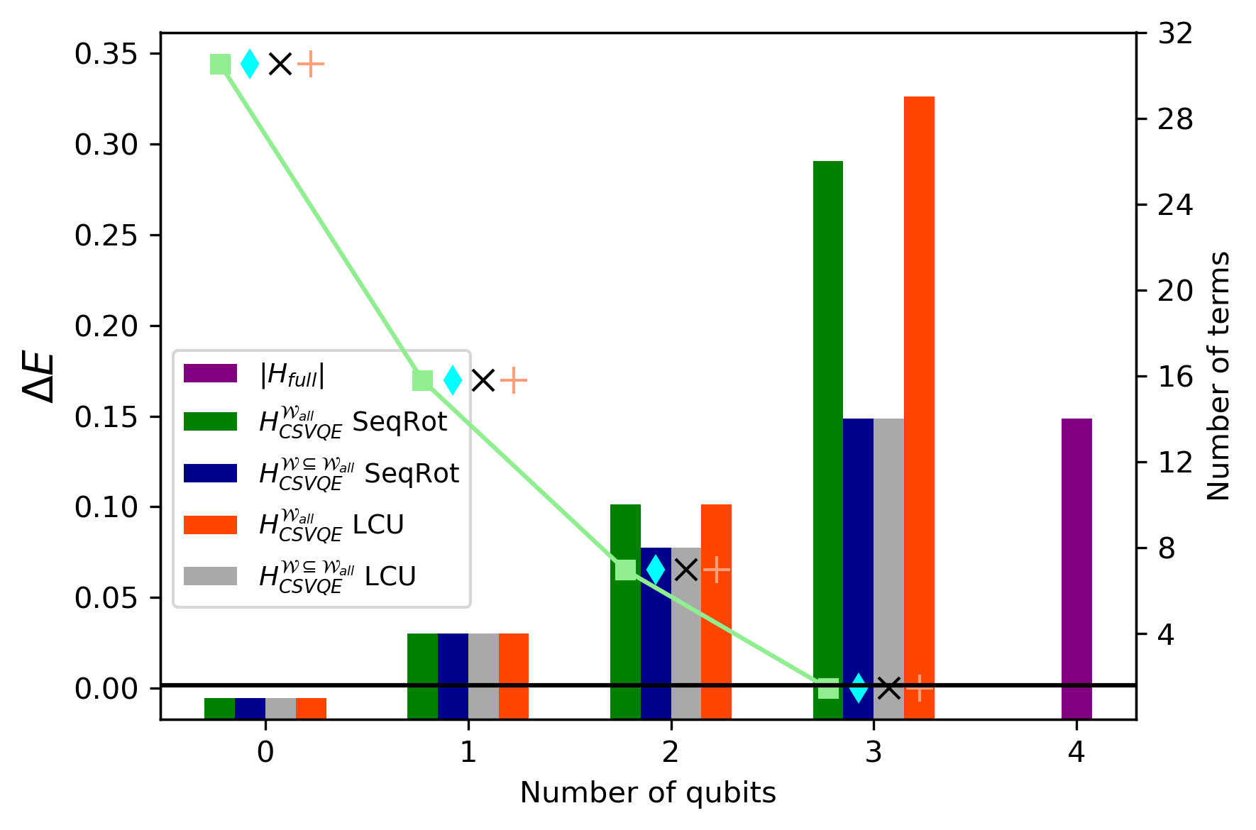
Overall four Hamiltonians are generated, representing different levels of approximation, that act on $0$, $1$, $2$ and $3$ qubits respectively. The $4$ qubit case represents the standard VQE on the full Hamiltonian. Figure ?? summarizes the error $\Delta E$ of each of these compared with the true ground-state energy (scatter plot). The number of terms in each Hamiltonian is given by the bar chart. The green and orange results have $\mathcal{W}\equiv\mathcal{W}_{all}$ for all cases and represent the old CS-VQE implementation. For these results, in the $3$ and $4$ qubit Hamiltonians have an increased number of terms due to $R_{S/LCU}$ being implemented, even though the eigenvalue of $\mathcal{A}(\vec{r}_{0})$ is not being fixed to $+1$. On the other hand, the gray and blue results in Figure ?? build $U_{\mathcal{W}}$ according to Equation ??, where $\mathcal{W}\subseteq\mathcal{W}_{all}$. This approach ensures that $R_{S/LCU}$ is only applied when necessary.

Figures ?? and ?? summarize the results of applying the unitary partitioning measurement reduction strategy to a set of electronic structure Hamiltonians We report the number of terms and number of qubits in each Hamiltonian required to achieve chemical accuracy compared with the original problem. The Supplemental Material gives further information about each result, where the different levels of noncontextual approximation are shown Sup. As previously discussed in Kirby et al. 2021, even though CS-VQE in general is an approximate method, chemical accuracy can still be achieved using significantly fewer qubits. Applying unitary partitioning on-top of the reduced CS-VQE Hamiltonians required to achieve chemical accuracy can further reduce the number of terms by roughly an order of magnitude. This is consistent with the previous results in Ralli et al. 2021.

To actually obtain a measurement reduction, one needs to show that the number of measurement required to measure the energy of a molecular system, to a certain precision $\epsilon$, is reduced. Currently, Figure ?? only shows that we have reduced the number of Pauli terms being measured. We have not commented on the variance. In the Supplemental Material Sup, we prove that simultaneous measurement of normalized anticommuting cliques can never do worse than performing no measurement reduction and will more often than not give an improvement. The proof given is state independent. There are other measurement strategies based on grouping techniques, such as splitting a Hamiltonian into commuting or qubit-wise commuting cliques Crawford et al. 2021; Gokhale and Chong 2019; Gokhale et al. 2019; Verteletskyi et al. 2020; Kandala et al. 2017. The measurement reduction obtained from these methods is more complicated, as the covariance of operators within a clique must be carefully accounted for McClean et al. 2016; Gokhale et al. 2019. This is one of the reasons we do not analyze the performance of these strategies in this paper. Many other measurement methods have also been proposed Izmaylov et al. 2019; Cotler and Wilczek 2020; Bonet-Monroig et al. 2020; Jena et al. 2019; Huggins et al. 2021; Crawford et al. 2021; Huang et al. 2020; Hadfield et al. 2022; Huang et al. 2021; Rubin et al. 2018; Gonthier et al. 2022 and their effect on the number of measurements would be interesting to investigate.

In Table ??, we report the upper bound on the gate count required to implement measurement reduction as a sequence of rotations. The LCU method would require ancilla qubits and analysis of the circuit depth is more complicated. Further analysis can be found in Ralli et al. 2021. The number of extra coherent resources required to implement unitary partitioning measurement reduction is proportional to the size of each anticommuting clique a Hamiltonian is split into Ralli et al. 2021; Zhao et al. 2020. The sequence of rotations circuit depth scales as $\mathcal{O}\big(N_{s}(|C|-1)\big)$ single qubit and $\mathcal{O}\big(N_{s}(|C|-1)\big)$ CNOT gates, where $N_{s}$ is the number of system qubits and $|C|$ is the size of the anticommuting clique being measured. Table ?? reports the gate count upper bound for the largest anticommuting clique of a given CS-VQE Hamiltonian. We do not consider possible circuit simplifications, such as gate cancellations. To decrease the depth of quantum circuit required for practical application, we suggest finding nonoptimal clique covers; for example, if anticommuting cliques are fixed to a size of $2$, the resources required to perform $R_{S}$ are experimentally realistic for current and near-term devices, as only $\mathcal{O}(N_{s})$ single qubit and $\mathcal{O}(N_{s})$ CNOT gates are required Ralli et al. 2021.

The heuristic used to determine the operators in $H_{\text{noncon}}$ selected terms in the full Hamiltonian greedily by coefficient magnitude, while keeping the set noncontextual Kirby and Love 2020. The Hamiltonians studied here had weights dominated by diagonal Pauli operators, as the Hartree-Fock approximation accounts for most of the energy. This heavily constrains the operators allowed in $\mathcal{A}$. For the electronic structure Hamiltonians considered in this paper, we found in all cases that $|\mathcal{A}|=2$. In general, we do expect more commuting terms in $H_{\text{noncon}}$ than anticommuting terms. This is because there are more possible commuting Pauli operators defined on $n$ qubits compared with anticommuting operators ( $2^{n}$ vs $2n+1$). $\mathcal{G}$ will therefore in general be the larger contributor to the superset $\mathcal{R}$ (Equation ??).

In Figure ??, the CS-VQE bars have not been split into two for the case when $R$ is constructed as $R_{LCU}$ or $R_{S}$. This is due to $|\mathcal{A}|$ being $2$ in all cases, which is the special case when these operators ($R_{LCU}$ and $R_{S}$) end up being identical. In this instance $R$ has the form $R=\alpha I+i\beta P$ and thus the number of terms will only increase for every term in the Hamiltonian that $P$ anticommutes with. However, in general $|\mathcal{A}|$ will be greater than $2$ and the effect of $R$ can dramatically affect the number of terms in the resultant rotated Hamiltonian. We observe this in Fig. ?? of the toy example, where the $2$ and $3$ qubit CS-VQE Hamiltonians have had $U_{\mathcal{W}_{all}}$ applied to them even though the eigenvalue of $A(\vec{r})$ is not fixed. In that example, for the $3$ qubit approximation the sequence-of-rotations rotated Hamiltonian (green) actually has fewer terms than the LCU rotated operator (orange). This result is an artifact of the small problem size. In the Supplemental Material we show that the scaling will favor the LCU implementation, where the number of terms in a Hamiltonian can only increase quadratically, not exponentially, when performing the unitary partitioning rotation as a LCU rather than a sequence of rotations Sup.

In the Supplemental Material, we show the convergence of CS-VQE at different noncontextual approximations. The results illustrate that CS-VQE can converge to below chemical accuracy well before the case when no noncontextual approximation is made (full VQE). Results beyond convergence are included to show the different possible levels of approximation. In practice knowledge of the true ground-state energy is not known a priori and so using chemical precision to motivate the noncontextual approximation will not be possible. In this setting, a way to approach quantum advantage is to note that CS-VQE is a variational method. The quantum resources required can be expanded until the energy obtained by CS-VQE is lower than that coming from the best possible classical method. At this point, either the algorithm can be terminated or further contextual corrections can be added until the energy converges, at which point the algorithm should be stopped.