Joint Super-Resolution and Inverse Tone-Mapping:
A Feature Decomposition Aggregation Network and A New BenchmarkJournal: Pattern Recognition

Previous one-stage joint SR-ITM methods [3, 4] first decompose an input LR-SDR image $\bm{I}_{in}\in\mathbb{R}^{H\times W\times 3}$, where $H$ and $W$ are the height and width, into the base and detail components via guided image filtering [11], and enhance them separately by different network branches. However, the decomposition [11] is performed only on the input image with fixed hyperparameters, which is not robust to versatile scenarios. To generalize the decomposition from the specific image domain to the general feature domain, we propose a novel Feature Decomposition Block (FDB) to perform the separation of feature details and contrasts in a data-driven manner. The pipeline of the feature decomposition block is as shown in Fig. 2 (top-left).

The goal of our FDB block is to extract detail and base feature maps from the input feature $\bm{F}_{in}\in\mathbb{R}^{H\times W\times C}$ (e.g., extracted from the input LR-SDR image $\bm{I}_{in}$) for joint SR-ITM, where $C$ is the number of channels. A straightforward way to this goal is to individually perform base feature extraction from the whole feature map $\bm{F}_{in}$, and obtain the detail feature by subtracting the base feature from $\bm{F}_{in}$. To improve the computational efficiency, we propose to split the input feature $\bm{F}_{in}$, along the channel dimension, into two feature maps $\bm{F}_{in}^{\alpha}$ and $\smash{\bm{F}_{in}^{\beta}}$, both in $\mathbb{R}^{H\times W\times C/2}$. This also makes our FDB block lightweight for efficient model design. Then we extract the initial base feature $\bm{F}_{ini}^{base}\in\mathbb{R}^{H\times W\times C/2}$ from the feature map $\smash{\bm{F}_{in}^{\beta}}$ by a $1\times 1$ convolutional layer, followed by a $3\times 3$ convolutional layer to output the enhanced base feature $\bm{F}_{out}^{base}\in\mathbb{R}^{H\times W\times C/2}$ with larger receptive field. To extract and output the detail feature $\bm{F}_{out}^{detail}$, we subtract the initial base feature $\bm{F}_{ini}^{base}$ from the feature map $\bm{F}_{in}^{\alpha}$ by

In this way, our FDB block decomposes the input feature map $\bm{F}_{in}$ into the detail feature map and base feature map in a data-driven manner:

Next, we stack multiple FDB blocks into a cascade to exploit the power of multi-level decomposition for fine-grained feature extraction and separation.

To obtain fine-grained detail feature map and base feature map, we cascade several (e.g., $B$) FDB blocks into a Hierarchical Feature Decomposition Group (HFDG) to separate the input feature $\bm{F}_{in}$ into different levels of base and detail feature maps, as shown in Fig. 2 (top-right). Given the input feature $\bm{F}_{in}\in\mathbb{R}^{H\times W\times C}$, we employ the first FDB block (called FDB-1) to decompose it into the base feature $\bm{F}_{1}^{base}$ and detail feature $\bm{F}_{1}^{detail}$, both in $\mathbb{R}^{H\times W\times C/2}$. Then the base feature $\bm{F}_{1}^{base}$ is fed into the subsequent FDB block for next-level feature decomposition. In general, the $b$-th FDB block ($b\in\{2,...,B\}$) decomposes the base feature $\bm{F}_{b-1}^{base}\in\mathbb{R}^{H\times W\times C/2^{b-1}}$ from previous FDB block as

where $\bm{F}_{b}^{base}$ and $\bm{F}_{b}^{detail}$ (both in $\mathbb{R}^{H\times W\times C/2^{b}}$) are the output base and detail feature maps, respectively.

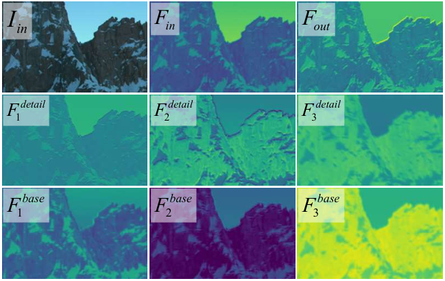
Thus far, we have multiple hierarchically decomposed base and detail feature maps. To well exploit their power for joint SR-ITM, we concatenate these features and refine them by a spatial attention mechanism. Since the base feature $\bm{F}_{b-1}^{base}$ ($b=2,...,B$) have been decomposed into next-level detail and base features, we only concatenate all the detail features $\bm{F}_{b}^{detail}$ ($b=1,2,...,B$) and the $B$-th base feature $\bm{F}_{B}^{base}$ to avoid redundancy on information and computational costs. Instead of the plain concatenation, here we choose to rescale the hierarchical feature maps from the FDBs and adaptively highlight the important regions in each hierarchical feature map according to the spatial distribution inside. Thus, we employ an Enhanced Spatial Attention (ESA) block introduced in [44] for spatial refinement aggregation:

where $[\cdot]$ denotes the concatenation operation and $\bm{F}_{out}$ is the output by HFDG group. Note that $\bm{F}_{out}\in\mathbb{R}^{H\times W\times C}$ is of the same size as the input feature $\bm{F}_{in}$. Considering that the ESA block [44] is not our contribution and not a key design in our main network, we put the detailed description of the ESA block [44] in the supplementary material.

In Fig. 3, we visualize the intermediate feature maps extracted by one HFDG with $B=3$ FDBs on the input LR-SDR image $\bm{I}_{in}$. From $\bm{I}_{in}$, we extract the input feature $\bm{F}_{in}$, and decompose it into different levels of detail features $\bm{F}_{b}^{detail}$ and base features $\bm{F}_{b}^{base}$ ($b=1,2,3$). As we can see, the three base features become coarser and coarser, and contain more and more structural information. This is reasonable since each base feature $\bm{F}_{b}^{base}$ is fused by a $3\times 3$ convolutional layer on that in the previous level. Similarly, by subtracting the base feature from that in the previous level, three detail features also become coarser and coarser. Finally, the multi-level detail and base features are integrated to produce an enhanced feature $\bm{F}_{out}$ with richer details and contrasts. This shows that our HFDG effectively integrates different levels of detail and structural base features.

With our HFDG group, we now develop a Feature Decomposition Aggregation Network (FDAN) for joint SR-ITM. The overall architecture is shown in Fig. 2 (bottom). Given the input LR-SDR image $\bm{I}_{in}\in\mathbb{R}^{H\times W\times 3}$, our FDAN network first extracts the initial feature $\bm{F}_{0}\in\mathbb{R}^{H\times W\times C}$ by a $3\times 3$ convolutional layer. Then, we cascade $G$ HFDG groups to extract the features $\bm{F}_{g}\in\mathbb{R}^{H\times W\times C}$ ($g\in\{1,...,G\}$) with different scales of receptive fields. The feature extracted by the $g$-th HFDG group (denoted as $\text{HFDG}_{g}$) is:

To fully exploit the multi-scale information for effective joint SR-ITM, we aggregate all these $G$ features $\{\bm{F}_{1},...,\bm{F}_{G}\}$ by direct concatenation, and integrate them by one $1\times 1$ convolutional layer and one $3\times 3$ convolutional operation. The resulting feature is added by the initial feature $\bm{F}_{0}$ via a long skip connection, to utilize the low-level detail information for visual-pleasing reconstruction. This can also stabilize and accelerate the training process of our FDAN network [6]. Finally, we reconstruct the HR-HDR image $\bm{I}_{out}\in\mathbb{R}^{sH\times sW\times 3}$ by a $3\times 3$ convolutional operation and a Pixel Shuffle operation [45] with the scale factor $s$.

Unless otherwise specified, in all experiments, we set the hyperparameters $C$, $B$, and $G$ in our FDAN as $C=48$, $B=3$, and $G=6$. Each convolutional layer contains a convolutional operation and a ReLU nonlinear function. We initialize our FDAN by the Kaiming initialization [46] without a pre-trained model. We utilize the Adam optimizer [47] with $\beta_{1}=0.9$ and $\beta_{2}=0.999$ to optimize our FDAN with the $\ell_{1}$ loss function. On the dataset introduced in the next section, we train our FDAN for 1,200 epochs (a total of 93,760 iterations) with the batch size of 64 for the scale factor of 4, 8 and 16 and the batch size of 32 for the scale factor of 2 due to the GPU memory limitation. The learning rate is initialized as $5\times 10^{-5}$ and decayed to $1\times 10^{-11}$ by a cosine annealing scheme [48] for every 120 epochs (9376 iterations). The training takes about 6.75 hours on a RTX 2080Ti GPU with 11GB memory.

Besides the official settings of LR-SDR and HR-HDR images with the scale factors of 2 and 4 provided in [3], we conduct additional SR-ITM settings with the scale factors of 8 and 16, to comprehensively evaluate the comparison methods on dataset in [3]. To obtain the LR-SDR images with the scale factors of 8 and 16, we downsample the LR-SDR images at the scale factor of 2 by a further scale factor of 4 and 8, respectively, through the standard bicubic interpolation. All models are retrained to achieve their corresponding best performance. The results of different competitors are listed in Table 2. One can see that our FDAN still outperforms the other one-stage SR-ITM methods [3, 4] in terms of PSNR and SSIM, but with the least parameters (model complexity) and lowest FLOPs (computational costs). This demonstrates the efficiency and effectiveness of our FDAN network over previous methods [3, 4] on joint SR-ITM.

Here, we provide comprehensive experiments to access: 1) effectiveness of our feature decomposition strategy; 2) the number of FDB blocks in an HFDG group; 3) the number of HFDG groups in our FDAN; 4) how feature aggregation contributes to our FDAN on joint SR-ITM. All the variants of our FDAN are trained on the SRITM-4K training set and evaluated on the SRITM-4K test set when the scale factor $s=4$.

References

- [1] I. Union, Recommendation itu-r bt. 2100-2, Electronic Publication (2016).
- [2] I. Union, Recommendation itu-r bt. 709-6, Electronic Publication (2015).
- [3] S. Y. Kim, J. Oh, M. Kim, Deep sr-itm: Joint learning of super-resolution and inverse tone-mapping for 4k uhd hdr applications, in: Int. Conf. Comput. Vis., 2019, pp. 3116–3125.
- [4] S. Y. Kim, J. Oh, M. Kim, Jsi-gan: Gan-based joint super-resolution and inverse tone-mapping with pixel-wise task-specific filters for uhd hdr video, in: Association for the Advancement of Artificial Intelligence, 2020, pp. 11287–11295.
- [5] C. Dong, C. C. Loy, K. He, X. Tang, Image super-resolution using deep convolutional networks, IEEE Trans. Pattern Anal. Mach. Intell. 38 (2) (2015) 295–307.
- [6] J. Kim, J. K. Lee, K. M. Lee, Accurate image super-resolution using very deep convolutional networks, in: IEEE Conf. Comput. Vis. Pattern Recog., 2016, pp. 1646–1654.
- [7] Y. Zhang, K. Li, K. Li, L. Wang, B. Zhong, Y. Fu, Image super-resolution using very deep residual channel attention networks, in: Eur. Conf. Comput. Vis., 2018, pp. 286–301.
- [8] G. Eilertsen, J. Kronander, G. Denes, R. K. Mantiuk, J. Unger, Hdr image reconstruction from a single exposure using deep cnns, ACM transactions on graphics (TOG) 36 (6) (2017) 1–15.
- [9] Y.-L. Liu, W.-S. Lai, Y.-S. Chen, Y.-L. Kao, M.-H. Yang, Y.-Y. Chuang, J.-B. Huang, Single-image hdr reconstruction by learning to reverse the camera pipeline, in: IEEE Conf. Comput. Vis. Pattern Recog., 2020, pp. 1651–1660.
- [10]
G. Wu, R. Song, M. Zhang, X. Li, P. L. Rosin,
Litmnet:
A deep cnn for efficient hdr image reconstruction from a single ldr image,
Pattern Recognition 127 (2022) 108620.
doi:https://doi.org/10.1016/j.patcog.2022.108620.
URL https://www.sciencedirect.com/science/article/pii/S0031320322001017 - [11] K. He, J. Sun, X. Tang, Guided image filtering, IEEE Trans. Pattern Anal. Mach. Intell. 35 (6) (2012) 1397–1409.
- [12] R. Zeyde, M. Elad, M. Protter, On single image scale-up using sparse-representations, in: Int. Conf. Curves and Surfaces, Springer, 2010, pp. 711–730.
- [13] J. Yang, J. Wright, T. S. Huang, Y. Ma, Image super-resolution via sparse representation, IEEE Transactions on Image Processing 19 (11) (2010) 2861–2873. doi:10.1109/TIP.2010.2050625.
- [14] R. Timofte, V. De Smet, L. Van Gool, A+: Adjusted anchored neighborhood regression for fast super-resolution, in: Asian Conf. Comput. Vis., Springer, 2014, pp. 111–126.
- [15] K. He, X. Zhang, S. Ren, J. Sun, Deep residual learning for image recognition, in: IEEE Conf. Comput. Vis. Pattern Recog., 2016, pp. 770–778.
- [16] G. Huang, Z. Liu, L. Van Der Maaten, K. Q. Weinberger, Densely connected convolutional networks, in: IEEE Conf. Comput. Vis. Pattern Recog., 2017, pp. 4700–4708.
- [17]
G. Li, M. Zhang, J. Li, F. Lv, G. Tong,
Efficient
densely connected convolutional neural networks, Pattern Recognition 109
(2021) 107610.
doi:https://doi.org/10.1016/j.patcog.2020.107610.
URL https://www.sciencedirect.com/science/article/pii/S0031320320304131 - [18]
B. Fu, Y. Li, X. hai Wang, Y. gong Ren,
Image
super-resolution using tv priori guided convolutional network, Pattern
Recognition Letters 125 (2019) 780–784.
doi:https://doi.org/10.1016/j.patrec.2019.06.022.
URL https://www.sciencedirect.com/science/article/pii/S0167865518308389 - [19]
P. V. Arun, I. Herrmann, K. M. Budhiraju, A. Karnieli,
Convolutional
network architectures for super-resolution/sub-pixel mapping of drone-derived
images, Pattern Recognition 88 (2019) 431–446.
doi:https://doi.org/10.1016/j.patcog.2018.11.033.
URL https://www.sciencedirect.com/science/article/pii/S0031320318304217 - [20]
N. Ahn, B. Kang, K.-A. Sohn,
deep neural network for photo-realistic image super-resolution, Pattern
Recognition 127 (2022) 108649.
doi:https://doi.org/10.1016/j.patcog.2022.108649.
URL https://www.sciencedirect.com/science/article/pii/S0031320322001303 - [21] C. Ledig, L. Theis, F. Huszár, J. Caballero, A. Cunningham, A. Acosta, A. Aitken, A. Tejani, J. Totz, Z. Wang, et al., Photo-realistic single image super-resolution using a generative adversarial network, in: IEEE Conf. Comput. Vis. Pattern Recog., 2017, pp. 4681–4690.
- [22] I. Goodfellow, J. Pouget-Abadie, M. Mirza, B. Xu, D. Warde-Farley, S. Ozair, A. Courville, Y. Bengio, Generative adversarial nets, Adv. Neural Inform. Process. Syst. 27 (2014).
- [23] J. Hu, L. Shen, G. Sun, Squeeze-and-excitation networks, in: IEEE Conf. Comput. Vis. Pattern Recog., 2018, pp. 7132–7141.
- [24]
P. Behjati, P. Rodriguez, C. Fernández, I. Hupont, A. Mehri, J. Gonzàlez,
Single
image super-resolution based on directional variance attention network,
Pattern Recognition 133 (2023) 108997.
doi:https://doi.org/10.1016/j.patcog.2022.108997.
URL https://www.sciencedirect.com/science/article/pii/S0031320322004770 - [25] A. Vaswani, N. Shazeer, N. Parmar, J. Uszkoreit, L. Jones, A. N. Gomez, Ł. Kaiser, I. Polosukhin, Attention is all you need, in: Adv. Neural Inform. Process. Syst., 2017, pp. 5998–6008.
- [26] X. Wang, R. Girshick, A. Gupta, K. He, Non-local neural networks, in: IEEE Conf. Comput. Vis. Pattern Recog., 2018, pp. 7794–7803.
- [27] Y. Mei, Y. Fan, Y. Zhou, Image super-resolution with non-local sparse attention, in: IEEE Conf. Comput. Vis. Pattern Recog., 2021, pp. 3517–3526.
- [28] H. Chen, Y. Wang, T. Guo, C. Xu, Y. Deng, Z. Liu, S. Ma, C. Xu, C. Xu, W. Gao, Pre-trained image processing transformer, in: IEEE Conf. Comput. Vis. Pattern Recog., 2021, pp. 12299–12310.
- [29] N. Ahn, B. Kang, K.-A. Sohn, Fast, accurate, and lightweight super-resolution with cascading residual network, in: Eur. Conf. Comput. Vis., 2018, pp. 252–268.
- [30] H. Zhao, X. Kong, J. He, Y. Qiao, C. Dong, Efficient image super-resolution using pixel attention, in: Eur. Conf. Comput. Vis., Springer, 2020, pp. 56–72.
- [31] X. Luo, Y. Xie, Y. Zhang, Y. Qu, C. Li, Y. Fu, Latticenet: Towards lightweight image super-resolution with lattice block, in: Eur. Conf. Comput. Vis., Springer, 2020, pp. 272–289.
- [32] Z. Hui, X. Gao, Y. Yang, X. Wang, Lightweight image super-resolution with information multi-distillation network, in: ACM Int. Conf. Multimedia, 2019, pp. 2024–2032.
- [33] J. Liu, J. Tang, G. Wu, Residual feature distillation network for lightweight image super-resolution, Springer, 2020, pp. 41–55.
- [34] F. Banterle, P. Ledda, K. Debattista, A. Chalmers, Inverse tone mapping, in: Proceedings of the 4th international conference on Computer graphics and interactive techniques in Australasia and Southeast Asia, 2006, pp. 349–356.
- [35] F. Banterle, P. Ledda, K. Debattista, A. Chalmers, M. Bloj, A framework for inverse tone mapping, The Visual Computer 23 (7) (2007) 467–478.
- [36] A. G. Rempel, M. Trentacoste, H. Seetzen, H. D. Young, W. Heidrich, L. Whitehead, G. Ward, Ldr2hdr: on-the-fly reverse tone mapping of legacy video and photographs, ACM transactions on graphics (TOG) 26 (3) (2007) 39–es.
- [37] S. Wu, J. Xu, Y.-W. Tai, C.-K. Tang, Deep high dynamic range imaging with large foreground motions, in: Eur. Conf. Comput. Vis., 2018, pp. 117–132.
- [38] N. K. Kalantari, R. Ramamoorthi, Deep high dynamic range imaging of dynamic scenes, ACM Trans. Graph. 36 (4) (2017).
- [39] G. Chen, C. Chen, S. Guo, Z. Liang, K.-Y. K. Wong, L. Zhang, HDR video reconstruction: A coarse-to-fine network and a real-world benchmark dataset, Int. Conf. Comput. Vis. (2021).
- [40]
R. Khan, Y. Yang, K. Wu, A. Mehmood, Z. H. Qaisar, Z. Zheng,
A
high dynamic range imaging method for short exposure multiview images,
Pattern Recognition 137 (2023) 109344.
doi:https://doi.org/10.1016/j.patcog.2023.109344.
URL https://www.sciencedirect.com/science/article/pii/S0031320323000456 - [41]
Q. Yan, D. Gong, J. Q. Shi, A. van den Hengel, J. Sun, Y. Zhu, Y. Zhang,
High
dynamic range imaging via gradient-aware context aggregation network,
Pattern Recognition 122 (2022) 108342.
doi:https://doi.org/10.1016/j.patcog.2021.108342.
URL https://www.sciencedirect.com/science/article/pii/S0031320321005227 - [42] M. S. Santos, R. Tsang, N. Khademi Kalantari, Single image hdr reconstruction using a cnn with masked features and perceptual loss, ACM Transactions on Graphics 39 (4) (7 2020). doi:10.1145/3386569.3392403.
- [43] X. Chen, Z. Zhang, J. S. Ren, L. Tian, Y. Qiao, C. Dong, A new journey from sdrtv to hdrtv, in: Int. Conf. Comput. Vis., 2021.
- [44] J. Liu, W. Zhang, Y. Tang, J. Tang, G. Wu, Residual feature aggregation network for image super-resolution, in: IEEE Conf. Comput. Vis. Pattern Recog., 2020, pp. 2359–2368.
- [45] W. Shi, J. Caballero, F. Huszár, J. Totz, A. P. Aitken, R. Bishop, D. Rueckert, Z. Wang, Real-time single image and video super-resolution using an efficient sub-pixel convolutional neural network, in: IEEE Conf. Comput. Vis. Pattern Recog., 2016, pp. 1874–1883.
- [46] K. He, X. Zhang, S. Ren, J. Sun, Delving deep into rectifiers: Surpassing human-level performance on imagenet classification, in: Int. Conf. Comput. Vis., 2015, pp. 1026–1034.
- [47] D. P. Kingma, J. Ba, Adam: A method for stochastic optimization, in: Int. Conf. Learn. Represent., 2015.
- [48] I. Loshchilov, F. Hutter, Sgdr: Stochastic gradient descent with warm restarts, Int. Conf. Learn. Represent. (2017).
- [49] L. Van der Maaten, G. Hinton, Visualizing data using t-sne, Journal of Mach. Learn. Res. 9 (11) (2008).
- [50] Z. Wang, A. C. Bovik, H. R. Sheikh, E. P. Simoncelli, Image quality assessment: from error visibility to structural similarity, IEEE Trans. Image Process. 13 (4) (2004) 600–612.
- [51] R. Mantiuk, K. J. Kim, A. G. Rempel, W. Heidrich, Hdr-vdp-2: A calibrated visual metric for visibility and quality predictions in all luminance conditions, ACM Trans. Graph. 30 (4) (2011) 1–14.
- [52] R. K. Mantiuk, M. Azimi, Pu21: A novel perceptually uniform encoding for adapting existing quality metrics for hdr, in: 2021 Picture Coding Symposium (PCS), IEEE, 2021, pp. 1–5.
- [53] X. Chen, Y. Liu, Z. Zhang, Y. Qiao, C. Dong, Hdrunet: Single image hdr reconstruction with denoising and dequantization, in: IEEE Conf. Comput. Vis. Pattern Recog. Worksh., 2021, pp. 354–363.
- [54] X.-T. Cheng, Pytorch-implemented-deep-sr-itm, https://github.com/greatwallet/Pytorch-Implemented-Deep-SR-ITM (2019).
- [55] K. Zhang, M. Danelljan, Y. Li, R. Timofte, J. Liu, J. Tang, G. Wu, Y. Zhu, X. He, W. Xu, et al., Aim 2020 challenge on efficient super-resolution: Methods and results, in: Eur. Conf. Comput. Vis., 2020, pp. 5–40.
Gang Xu received his B.Sc. degree in information security from Xidian University, China in 2018, and Ph.D. degree in computer science and technology from Nankai University, China in 2023.
Yu-Chen Yang received the B.Sc. degree from the School of Statistics and Data Science, Nankai University, Tianjin, China, in 2022, where he is currently pursuing the M.Sc. degree with the School of Statistics and Data Science.
Liang Wang received his Ph.D. degree from the Institute of Automation, Chinese Academy of Sciences (CASIA) in 2004. From 2004 to 2010, he has been working at Imperial College London, United Kingdom, Monash University, Australia, the University of Melbourne, Australia, and the University of Bath, United Kingdom, respectively. Currently, he is a full Professor at the National Lab of Pattern Recognition, CASIA.
Xian-Tong Zhen received the B.S. and M.E. degrees from Lanzhou University, Lanzhou, China in 2007 and 2010, respectively, and the Ph.D. degree from the Department of Electronic and Electrical Engineering, The University of Sheffield, U.K., in 2013. He is currently with University of Amsterdam and Inception Institute of Artificial Intelligence (IIAI).
Jun Xu received his B.Sc. and M.Sc. degrees from School of Mathematics Science, Nankai University, Tianjin, China, in 2011 and 2014, respectively, and Ph.D. degree from Department of Computing, Hong Kong Polytechnic University, in 2018. He worked as a Research Scientist at IIAI, Abu Dhabi, UAE. He is currently an Associate Professor with School of Statistics and Data Science, Nankai University.