Revealing the dust grain polarization properties as a function of extinction and distance towards NGC 18932022Revealing the dust grain polarization properties as a function of extinction and distance towards NGC 1893–A
Abstract
Dust polarization observations at optical wavelengths help to understand the dust grain properties and trace the plane-of-the-sky component of the magnetic field. In this study, we make use of the -band polarization data acquired from AIMPOL along with the distances () and extinction () data to study the variation of polarization fraction () as a function of and towards the star-forming region, NGC 1893. We employ a broken power-law fit and Bayesian analysis on extinction () versus polarization efficiency (/) and distance () versus rate of polarization (/). We find that / shows a break at an extinction of 0.9 mag, whereas exhibits a break at a distance of 1.5 kpc. Based on these, we categorize the dust towards NGC 1893 into two populations: (i) foreground dust confined to 1 mag and distance up to 2 kpc and (ii) Perseus spiral arm dust towards NGC 1893 characterized with 1 mag and distance beyond 2 kpc. Foreground dust exhibits higher polarization efficiency but a lower polarization rate, whereas Perseus dust shows a lower polarization efficiency but a slightly higher polarization rate. Hence, we suggest that while polarization efficiency reveals the dust grain alignment, the rate of polarization infers about the distribution of dust grains towards NGC 1893. Further, we also shed a light on the spatial variation of intrinsic polarization and magnetic field orientation, and other parameters within the intra-cluster medium of NGC 1893.
Keywords:
polarization, dust, extinction, magnetic fields1 Introduction
Interstellar dust polarization has been studied extensively for more than half a century since it was observed for the first time at visible wavelengths by Hall 1949 and Hiltner 1949a. It has been proposed that the observed polarization was caused by the dichroic extinction of asymmetrical dust grains, which are aligned with respect to the Galactic magnetic field (Hiltner 1949b; Davis Jr & Greenstein 1951).
Since magnetic alignment of the dust grains is a prerequisite for the interstellar polarization to occur, several mechanisms have been proposed to explain it (Andersson et al. 2015, see,). Nevertheless, most of the theoretical and experimental evidence points towards the radiative alignment torque (RAT) mechanism as the most probable mechanism for dust grain alignment, which can then explain the observed optical/NIR and far-infrared/millimeter polarization in the interstellar medium (Lazarian 2007; Lazarian & Hoang 2007; Andersson et al. 2011). According to the RAT mechanism, when the radiation incidents upon an irregular dust grain, there is a difference in the extinction cross-sections experienced by the left circular and right circular polarization components of the incident light. This results in the generation of radiative torques which act on the grains, causing them to spin up due to increased angular momentum. In the presence of an external magnetic field, the grains Larmor precesses around the magnetic field, and the radiative torques acting over the precessing period align the grains with the field (Dolginov & Mytrophanov 1976; Draine & Weingartner 1996; Draine & Weingartner 1997).
When the background starlight passes through these magnetically aligned dust grains, its electric vector parallel to the long axis of the dust grains encounter a maximum extinction cross-section as compared to that parallel to the short axis. This differential extinction cross-section causes the transmitted starlight through the dust grains to be partially plane-polarized up to a few percent. The observed polarized light yield, two important parameters – (i) fraction of polarization (), which reveals the averaged dust grain properties along the line of sight (LOS), and (ii) polarization angle (), which reveals the LOS averaged magnetic field projected on the plane of the sky (POS) (Davis Jr & Greenstein 1951; Lazarian & Hoang 2007).
It has been observed that in optical -band, the observed polarization, , increases with total extinction (), and the distribution for various lines of sight suggest, an upper limit of < 3% mag-1 (Serkowski et al. 1975). A key conclusion from these data is that does not increase in the same proportion as does, owing to several factors that include (i) the properties of dust grains themselves such as the grain size (e.g, 0.1 – 0.3 µm), shape (e.g, oblate or prolate), composition (e.g, silicate, graphite or graphite-silicate), mantle to core volume ratio, presence or absence of surface coatings, (ii) magnetic field orientation weighted according to the distribution of dust grains along the line of sight, (iii) the efficiency of grain alignment, and (iv) inclination angle between the actual magnetic field with respect to LOS, and (v) the physical conditions of the environment in which dust exist (Lee & Draine 1985, see). Therefore, observed polarization measurements need to be critically analysed before interpreting the data.
One of the key concerns is to know whether the polarization measurements of a distant target would reveal the dust grain properties and magnetic field orientation of foreground dust only, but not of intra-cluster medium of a distant cluster, or all the dust grains along the line of sight to the target. To be specific about what regime of is responsible for the observed polarization observations, one of the promising approaches would be analysing the variation of the ratio , the dust grain polarization efficiency, as a function of , e.g, by means of a power-law fit of the form . The power-law index at different ranges of hints at dust grain alignment efficiency at those corresponding layers of dust. For example, corresponds to the total loss of dust grain alignment, and corresponds to the efficiently aligned dust grains at all optical depths (Pattle et al. 2019, e.g,). These interpretations are similar to those based on the index in the relation , where and are the dust emission polarization and intensity, respectively at sub-millimeter wavelength (Jones et al. 2015; Wang et al. 2019; Pattle et al. 2019, e.g,). The study of polarization efficiency at various wavelengths has been the subject of research (Goodman et al. 1992; Goodman et al. 1995; Gerakines et al. 1995; Andersson & Potter 2005; Franco et al. 2010; Wang et al. 2017). The majority of these studies have shown that varies as a function of with the values ranging from about 1 to 0.5.
In this work, we examine the relation between versus towards the direction of a prominent star forming region NGC 1893, located at a distance of 3.2 kpc (Kharchenko et al. 2005), with an average age of 23 Myr (Massey et al. 1995). NGC 1893 is an active star forming region hosting young massive O/B type stars and two elephant trunk-like nebulae Sim 129 and 130 shown in Figure 1. Therefore, it is an interesting region to study the dust properties and magnetic field orientations influencing star formation and polarization. This region has been investigated extensively over several years (Gaze & Shajn 1952; Massey et al. 1995; Marco & Negueruela 2002; Maheswar et al. 2007; Sharma et al. 2007) and has existing polarization data (Eswaraiah et al. 2011).
Another critical parameter that can be used to study the dust properties is the ratio of polarization to distance, , as a function of distance () along a particular LOS. is known as the rate of polarization. This relation is analogous to the rate of extinction, , that is, the ratio of visual extinction () to distance (), the mean of which is found to be 1.8 mag kpc-1 (Whittet 2018, see,). Recently, several researchers (Eswaraiah et al. 2011; Kumar et al. 2014; Wang et al. 2017; Lee et al. 2018; Eswaraiah et al. 2019; Kumar et al. 2019, e.g.,) have studied the variation of using the polarization data from Heiles 2000 and distances from Hipparchus catalogue (Van Leeuwen 2007) to show that increases as a function of distance towards several targets in the solar neighbourhood. A common limitation of all such studies have been that they are confined to the solar neighbourhood or to particular distances where the clusters are located. In this context, studying as a function of distance towards NGC 1893, being at a long distance beyond the solar neighbourhood, can shed light on the distribution of polarizing dust grains and presence of dust clouds along the LOS. It can also help to distinguish the foreground dust from that in the intra-cluster medium by revealing the distance at which the shows a change.
Eswaraiah et al. 2011 have observed a constant magnetic field orientation beyond 1 kpc along the direction of NGC 1893. It was uncertain whether this is due to the uniform and dominant magnetic field in the foreground dust medium, or a truly constant field all up to the distance of NGC 1893. The revised distances determined from the recent Gaia EDR3 observations for both foreground and background fields and cluster members plus the polarization data provides an opportunity to study the variation of polarization and magnetic fields as a function of distance for a statistically significant sample of stars. It is possible to correct for the foreground contribution in the stokes vector form and therefore to study the variation in the dust properties and magnetic fields within a distant cluster. In this work, in addition to versus , we also examine versus utilizing the newly acquired polarization data along with the existing data (Eswaraiah et al. 2011), stellar distances from Gaia EDR3 (Bailer-Jones et al. 2021), and the extinction values from Bayestar19 three-dimensional (3D) dust map (Green et al. 2019).
Section 2 describes our new observations, and data reduction, in addition to archival data. Section 3 presents the analyses. Results are given in Section 4, including the fit with the broken power-law and Bayesian analyses on – and – plots, foreground subtraction, magnetic field morphology in NGC 1893, and the variation of various parameters of the confirmed cluster members as a function of radial distance, etc. We discuss our results in Section 5. Finally, Section 6 summarizes our findings and gives the conclusions.
2 Observations and data reduction and archival data
2.1 Polarization data from ARIES IMaging POLarimeter (AIMPOL)

Deeper -band polarimetry observations of three fields towards NGC 1893 were carried out using the ARIES Imaging Polarimeter (AIMPOL) (Rautela et al. 2004, ) on 04 November 2013, mounted on the Cassegrain focus of the 104 cm Sampurnanand Telescope at ARIES in Nainital, India. In addition, we also reanalysed the six fields of -band data towards NGC 1893 acquired on the two nights of 08 and 09 November 2008. The detailed reduction and analysis procedures of AIMPOL data can be found in Eswaraiah et al. 2011; Eswaraiah et al. 2012; Eswaraiah et al. 2013. Figure 1 depicts the field around NGC 1893. The six fields observed in 2008 and three fields in 2013 are indicated. Instrumental polarization of AIMPOL has been consistently estimated to be less than 0.1 (Eswaraiah et al. 2011; Eswaraiah et al. 2012, cf. ). The offset in the polarization angle is determined by observing the polarized standard star HD 25443 on 04 November 2013 for which the polarization and polarization angle in -band are estimated 4.160.10 and 1341, respectively, consistent with the standard polarization 4.250.04 and polarization angle 134.20.3 in -band for HD 25443 (Schmidt et al. 1992). All the polarization measurements, acquired on 04 November 2013, are corrected for the instrumental polarization and offset in the polarization angle. We found 40 common stars observed in both years of 2008 and 2013. The values of polarization (Top) and polarization angles (Bottom) measured in 2008 and 2013 are found to match closely with each other, as shown in Fig. 2. The stars shown with encircled filled circles are the two H sources (Maheswar et al. 2007) and two Class II/Class III sources (Pandey et al. 2014). The measurements made in 2013 have smaller uncertainties owing to longer exposure time than those measured in 2008. Therefore, we adopt the measurements of 2013 for common sources in both epochs, and for the sources otherwise detected in only one epoch, we use the corresponding epoch data in our analysis.

Before we perform the analyses, we exclude the stars with possible intrinsic polarization based on the near-infrared (NIR) colour-colour diagram. Here, we assume that the intrinsic polarization can only be caused by the stars with circumstellar disks. Figure 3 shows the [J-H] vs [H-Ks] NIR colour-colour diagrams for 173 stars in -band whose signal-to-noise ratio in polarization, , is greater than 3, i.e, possibly with intrinsic polarization. The photometric data have been obtained from 2MASS Point Source Catalogue (Cutri et al. 2003). Red and blue-filled circles are the Class II and Class III sources (Pandey et al. 2014). Small green-filled circles are the H sources (Maheswar et al. 2007). Other NIR-excess sources are represented with encircled filled circles. In total, 21 stars, as mentioned above, may have intrinsic polarization. Therefore, out of 173 stars, we utilize the polarization data of 152 stars for the analyses. Figure 3 shows that most stars are not highly extincted, but rather are distributed around the main sequence (MS) locus, with a few along the giant locus.

2.2 Distances from GAIA Early Data Release 3
We obtain the distances from Bailer-Jones et al. 2021. They have estimated distances using stellar parallaxes of 1.47 billion stars and have published Gaia Early Data Release 3 (hereafter Gaia ERD3). Even though Gaia ERD3 have a significant improvement in both precision and accuracy of astrometry and broad-band photometry, the majority of these stars are distant or faint that their parallax uncertainties are large, thereby precluding a simple inversion of stellar parallax to provide a distance. Therefore, they use a probabilistic approach to estimate the stellar distances using a prior constructed from a three-dimensional model of our galaxy, which includes the interstellar extinction and Gaia’s variable magnitude limit. Using this method, Bailer-Jones estimate two types of distances: (i) Geometric and (ii) Photogeometric. The first one uses the parallax together with a direction-dependent prior on distance, whereas the second one additionally uses the colour and apparent magnitude of a star, by exploiting the fact that stars of a given colour have a restricted range of probable absolute magnitudes and extinction. There exist geometric distances for 1.47 billion stars, and 92% of these stars have photogeometric distances. Tests on simulated data and external validation show that the photogeometric estimates generally have higher accuracy and precision for fainter and distant stars (Bailer-Jones et al. 2021). Therefore, we utilize photogeometric distances for our study. We cross-match the coordinates of 152 stars having polarization data with the Bailer-Jones catalogue towards NGC 1893. Within a 0.5 matching radius, we find 151 stars have photogeometric distances. They are given in Table 1.
2.3 Extinction data
We use the total extinction at V-band, , data for our analyses. data are extracted from Green et al. 2019. They use stellar photometry from optical Pan-STARRS 1 and near-infrared 2MASS photometry along with the Gaia DR2 parallaxes to infer distances and reddening to 800 million stars. The reddening values of these stars are traced along different lines of sight, based on which they build a map of dust reddening in three-dimensions (Green et al. 2019) referred to as Bayestar19. Extinction towards a particular line of sight but at different distances can be extracted using the Python based module, dust maps11 1 {https://dustmaps.readthedocs.io/en/latest/modules.html##module-dustmaps.bayestar}. The extinction map is structured as a set of sight lines, each of which contains multiple samples of cumulative dust reddening as a function of distance. Each sight line is identified by a HEALPix nside parameter and a nested pixel index. Within each sight line, cumulative reddening is given at discrete distances, spaced evenly in the distance modulus. Thus, for each pixel, it provides multiple samples from the posterior of dust reddening. It also gives quality assurance information for each pixel, i.e., whether the fit converges in the pixel and the minimum/maximum reliable distance moduli in the pixel (Green et al. 2019)22 2 {https://dataverse.harvard.edu/dataset.xhtml?persistentId=doi:10.7910/DVN/2EJ9TX}.
We use the above-mentioned Python package ‘dust maps’ which provides functions for querying and downloading the Bayestar19 3D dust map. The reddening values from the Bayestar19 dust map are obtained by providing the equatorial coordinates of stars and their distances as input. Thus, the reddening values corresponding to the maximum posterior density at a particular coordinate and distance are returned as output. Finally, the obtained reddening values are checked for their quality by examining whether the line-of-sight fit has converged in a given pixel and also whether the input distance is reliable within the range of the considered distances. Hence, we find the reddening values for 151 stars. Of which, 8 do not have reliable distance information, although their line-of-sight fits are converged. These eight stars are excluded from further analyses. Thus, the obtained reddening values for 143 stars are converted into extinctions using the following relations (Green et al. 2019) 33 3 {http://argonaut.skymaps.info/usage##units}:
| (1) |
where is the reddening value obtained from Bayestar19 3D dust map. The and are the reddening values corresponding to and colours, is the total extinction in the visual band, and is the total-to-selective extinction of 3.1 (Savage & Mathis 1979; Cardelli et al. 1989). Since the dustmaps module does not provide uncertainties in reddening values, they are extracted from Galactic Interstellar Extinction (GALExtin44 4 www.galextin.org; Amôres et al. 2021).
The maximum distance up to which the Bayestar19 3-D extinction map reddening values are reliable are estimated based on the distance at which the main sequence stars disappear along a particular LOS (Green et al. 2019). Since the stellar cluster NGC 1893 which is the subject of our study has a galactic latitude of -1.6342°, and is located close to the galactic midplane, the stellar number density in this region is significantly high (Sharma et al. 2007, see, Figure 6 (a) of). So, there won’t be any dearth of main sequence stars at a particular distance along any LOS in this region. So the extinction () values we have extracted are valid up to a maximum of distance of 7 kpc which is the maximum photogeometric distance that we have used in our study.
To check the reliability of our reddening values obtained from Bayestar19 dust map (Green et al. 2019) , we compare our reddening values with those from Bayestar15 (Green et al. 2015), Bayestar17 (Green et al. 2018) and Chen2019 (Chen et al. 2019) dust maps. Bayestar15 is a 3D map of dust reddening using Pan-STARRSS 1 and 2MASS photometry based on a probabilistic approach, covering over a three-quarters of the sky. Bayestar17 is an improved version of Bayestar15 with the inclusion of additional Pan-STARRS 1 data, updated methodology and finer angular resolutions at high extinction regions. Chen2019 is another all sky map of dust reddening in 3D computed using the parallax and optical photometry from Gaia DR2 and infrared photometry from 2MASS and WISE. We find that most of our reddening values have a one to one correspondence with the reddening values obtained from these three dust maps, thereby attesting that our reddening values are reliable, and these data are also given in Table 1.
2.4 Dust temperature using IRAS data
One of the key predictions of RAT theory is the positive correlation between the degree of polarization and dust temperature (Lazarian & Hoang 2007; Andersson et al. 2015). In order to examine whether this relation exists in NGC 1893 region, we extract the dust temperature map. Since the current target does not have Herschel data, we use Infrared Astronomical Satellite (IRAS) maps at 60 and 100 m taken from SkyView Virtual observatory55 5 https://skyview.gsfc.nasa.gov/current/cgi/titlepage.pl. The dust temperature in each pixel of the IRAS image is obtained by assuming that the dust in a single beam is isothermal and that the observed ratio of 60 to 100 m emission follows a blackbody radiation from dust grains at temperature , modified by a power-law emissivity spectral index . We use the following relation to derive (Schnee et al. 2005):
| (2) |
where is the ratio of 60 to flux densities, is the dust emissivity spectral index which is approximately taken as 2, and is the dust temperature at each pixel of the IRAS image. We cross-match the list of cluster stars having polarization measurements with the pixels of map. Since the resolution of IRAS 60/100 m, and hence the map, is 2′, we estimate mean and standard deviation in over the pixels within 2′ diameter around each star having polarization data.
| SNo | Year | RA (J2000) | Dec (J2000) | Distance | P | PA |
|---|---|---|---|---|---|---|
| (degree) | (degree) | (kpc) | (%) | (degree) | ||
| 1 | 2008 | 80.665346 | 33.371732 | 3.00 0.16 | 2.12 0.18 | 151.0 2.0 |
| 2 | 2008 | 80.723805 | 33.392084 | 2.22 0.10 | 2.15 0.48 | 167.0 6.0 |
| 3 | 2008 | 80.719046 | 33.386870 | 2.32 0.12 | 2.37 0.49 | 164.0 6.0 |
| 4 | 2008 | 80.717592 | 33.384285 | 2.35 0.15 | 2.54 0.31 | 162.0 4.0 |
| 5 | 2008 | 80.688602 | 33.371345 | 0.86 0.01 | 1.46 0.23 | 174.0 4.0 |
| 6 | 2008 | 80.699181 | 33.368585 | 0.94 0.02 | 1.65 0.38 | 175.0 7.0 |
| 7 | 2008 | 80.741272 | 33.368718 | 2.68 0.78 | 2.79 0.49 | 158.0 5.0 |
| 8 | 2008 | 80.771703 | 33.359300 | 2.87 0.16 | 2.23 0.63 | 156.0 8.0 |
| 9 | 2008 | 80.622089 | 33.514012 | 3.01 0.21 | 2.86 0.12 | 147.0 1.0 |
| 10 | 2008 | 80.699321 | 33.476143 | 0.84 0.01 | 1.88 0.21 | 165.0 3.0 |
| 11 | 2008 | 80.751907 | 33.496616 | 2.51 0.12 | 2.79 0.27 | 161.0 3.0 |
| 12 | 2008 | 80.731302 | 33.487467 | 3.10 0.25 | 3.39 0.58 | 159.0 5.0 |
| 13 | 2008 | 80.767385 | 33.470600 | 2.92 0.17 | 3.12 0.48 | 155.0 4.0 |
| 14 | 2008 | 80.725975 | 33.445086 | 2.81 0.16 | 3.00 0.59 | 154.0 6.0 |
| 15 | 2008 | 80.782324 | 33.467270 | 2.14 0.12 | 2.82 0.54 | 159.0 6.0 |
| 16 | 2008 | 80.762063 | 33.454518 | 1.63 0.08 | 2.25 0.69 | 159.0 9.0 |
| 17 | 2008 | 80.741849 | 33.443460 | 1.47 0.50 | 2.36 0.26 | 160.0 3.0 |
| 18 | 2008 | 80.713246 | 33.426608 | 3.29 0.28 | 3.03 0.73 | 150.0 7.0 |
| 19 | 2008 | 80.744290 | 33.400895 | 2.73 0.22 | 3.47 0.52 | 160.0 4.0 |
| 20 | 2008 | 80.765901 | 33.400821 | 3.28 0.20 | 2.90 0.46 | 161.0 5.0 |
| SNo | J | H | K | Temperature | |
|---|---|---|---|---|---|
| (mag) | (mag) | (mag) | (mag) | (K) | |
| 1 | 9.00 0.02 | 8.89 0.02 | 8.79 0.02 | 1.67 0.12 | 28.72 0.77 |
| 2 | 11.58 0.02 | 11.57 0.02 | 11.54 0.02 | 0.79 0.02 | - |
| 3 | 11.82 0.02 | 11.76 0.02 | 11.71 0.02 | 0.79 0.02 | - |
| 4 | 11.02 0.02 | 10.99 0.02 | 10.99 0.02 | 0.79 0.02 | - |
| 5 | 10.13 0.03 | 10.06 0.02 | 9.99 0.02 | 0.63 0.1 | - |
| 6 | 10.92 0.02 | 10.58 0.02 | 10.49 0.02 | 0.63 0.1 | - |
| 7 | 11.91 0.02 | 11.82 0.02 | 11.81 0.02 | 1.07 0.09 | - |
| 8 | 11.44 0.02 | 10.70 0.02 | 10.50 0.02 | 1.24 0.11 | - |
| 9 | 8.28 0.02 | 8.25 0.03 | 8.18 0.02 | 1.07 0.09 | 30.87 0.31 |
| 10 | 8.82 0.02 | 8.22 0.02 | 8.06 0.02 | 0.68 0.02 | - |
| 11 | 11.64 | 11.53 | 11.43 0.03 | 0.79 0.05 | - |
| 12 | 12.48 0.02 | 12.09 0.02 | 11.94 0.02 | 1.15 0.05 | 31.21 0.4 |
| 13 | 12.77 | 12.57 0.05 | 12.47 0.04 | 0.88 0.07 | - |
| 14 | 12.80 0.03 | 12.68 0.04 | 12.62 0.03 | 0.87 0.05 | - |
| 15 | 12.48 0.02 | 12.31 0.03 | 12.24 0.02 | 0.83 0.02 | - |
| 16 | 12.77 0.02 | 12.43 0.02 | 12.34 0.02 | 0.82 0.02 | - |
| 17 | 11.46 0.02 | 11.32 0.02 | 11.26 0.02 | 0.82 0.03 | - |
| 18 | 13.44 0.03 | 13.33 0.04 | 13.22 0.04 | 2.16 0.04 | 30.58 0.64 |
| 19 | 12.40 0.02 | 12.26 0.02 | 12.21 0.02 | 0.86 0.07 | - |
| 20 | 11.90 0.02 | 11.24 0.02 | 11.05 0.02 | 1.15 0.08 | 31.64 0.53 |
3 analyses
In this section we analyse how the polarization efficiency () varies as a function of extinction () and (ii) rate of polarization () varies as a function of distance (). We used these analyses to examine whether the observed polarization measurements reveal the dust properties and magnetic field orientation of the foreground medium alone but not of the intra cluster medium, or of the dust grains distributed along the entire line of sight towards NGC 1893. After confirming the latter one that our polarization measurements consist of a contribution from the magnetically aligned dust grains in the intra-cluster medium, we try to quantify the foreground polarization contribution and subtract it from the measurements of cluster members. Eventually, we examine if there are changes in intrinsic polarization parameters, dust temperature, extinction, and polarization efficiency within the cluster region.
We model the plots with two different methods: – (i) broken power-law with a Levenberg-Marquardt non-linear least squares fitting method and (ii) broken power-law but with a Bayesian approach.
3.1 Broken Power-law fit
The relation – is fitted with broken power-law of the form using module in Python:
| (3) |
where is , is the at which the power-law breaks, and is a coefficient. The and are power-law indices before and after . Similarly, the data of – are also fitted with the broken power-law of the similar form to equation 3, where and are replaced with distance () and distance break at which the power-law breaks, respectively. Figure 4 show the data and corresponding best fits for – and – , respectively. The best-fit parameters are given in Table 2.
To check whether the broken power-law model of – and – fit the data better than a single power-law, we perform -difference test and also estimate Akaike Information Criterion (AIC) and Bayesian Information Criterion (BIC) values. For – with the difference in the degrees of freedom 2, the -difference is 9.255 which is statistically significant as the corresponding p-value turns out to be 0.01 which is less than the statistically accepted 0.05 significance level, meaning that the model with more free-parameters or the broken power-law fits the data better. Furthermore, the AIC and BIC values for the broken power-law are lower than that of single power-law fit, confirming that the broken power-law is a better model than single power-law for – . For – again with the difference in the degrees of freedom 2, the -difference is 1.032, which is statistically insignificant as the corresponding p-value turns out to be 0.6 which is greater than the significance level of 0.05, implying that both models fit the data equally well. But lower values of AIC and BIC when compared to that of single power-law suggests that the broken power-law fits the data better. Therefore, broken power-law model can be accepted for fitting both – and – relations.


| Relation | or | |||
|---|---|---|---|---|
| – | 2.6 0.2 | 0.01 0.19 | -1.0 0.1 | 0.96 0.09 mag |
| – | 1.1 0.1 | -0.8 0.1 | -0.3 0.1 | 1.5 0.3 kpc |
3.2 Bayesian Analyses
We have employed Bayesian analyses to confirm the results obtained from the broken power-law for – and – (above section). Bayesian analyses can help constrain the posterior distribution of all parameters based on the prior distributions and observational data expressed in the form of a likelihood function. We modeleled the trends followed by – and – by combining broken power-law with Bayesian approach. The resulting analyses yield us the posterior mean fit along with the 95%, 68%, and 50% confidence regions (CRs), and the posterior probability density function (PDF) of each parameter as output as described in appendix A. The 95%, 68%, and 50% confidence regions (CRs) predicted by the posterior distribution for – and – plots are shown in Figure 5. From the figures, it is seen that the majority of the data fall well within 95% CR predicted by the posterior. The 94 % highest density interval (HDI) of each parameter are plotted to represent the data lying within 2 uncertainties. The posterior PDF of the parameters derived from the Bayesian modelling is given in Figure 6. In Figure 6, is a constant, , and are the power-law indices before and after the break in power-law for both the – . and – plots. and are the and values at which the break occurs in – and – respectively. Similarly, is the dispersion in the data of or . More details about various parameters are given in the appendix A. The parameters constrained through the Bayesian analyses are reasonably more accurate than those obtained from the broken power-law alone. The constrained results from Bayesian analyses are listed in Table 3.
| Relation | 3% HDI () | 97 % HDI () | 3% HDI () | 97 % HDI () | or | 3% HDI ( or ) | 97 % HDI ( or ) | ||||
|---|---|---|---|---|---|---|---|---|---|---|---|
| – | 2.8 | 0.04 | -0.26 | 0.18 | -0.9 | -1.2 | -0.7 | 0.9 mag | 0.8 mag | 1 mag | 0.6 %/mag |
| – | 1.3 | -0.8 | -0.9 | -0.6 | -0.6 | -0.7 | -0.4 | 1.5 kpc | 0.8 kpc | 2.3 kpc | 0.3 %/kpc |
- •
HDI: Highest density interval


3.3 Differential plots in P and PA as a function of distance
Stokes parameters ( and ) of all 151 stars are converted from and (see, section 2.1) using the relations:
| (4) |
To understand the change in polarization parameters in response to the dust layers along the line of sight, we construct differential plots in Stokes parameters ) and ) versus distancei+1, where is an immediate foreground star to star. These and are converted into and using the relations:
| (5) |
The corresponding errors are given by:
| (6) |
These analyses help visualize the changes in and across the dust layers lying between and star (see Eswaraiah et al. 2019).


The differential density plots shown in the Figure 7 reveal a clear transition in both and at a distance of 2 kpc. To elucidate further, the information on probability density and frequency distribution are shown with gray/black background and histograms, respectively. Note that while constructing histograms we use bin sizes of 0.25%, 10, and 350 pc for , , and distancei+1 respectively.
To confirm this transition occurring at a distance of 2 kpc, we apply the Gaussian Mixture Model (GMM) analyses (Krone-Martins et al. 2010; Ducourant et al. 2017; Melchior & Goulding 2018; Cantat-Gaudin et al. 2019, e.g,) on the differential plots, by providing , , and, distancei+1 as input using the module in python. GMM is a probabilistic model which assumes that the data instances are generated from several Gaussian distributions each with an unknown set of parameters, i.e, mean and covariance values. Since GMM is a powerful grouping algorithm, we use it for grouping stars based on their properties. The GMM does this by assigning probability for each star being part of a separate group, say group-0 or group-1. For this purpose, GMM uses an Expectation-Maximization (EM) algorithm. The EM algorithm starts off by assigning the group parameters randomly to the given set of stars and is followed by two steps: expectation and maximization, which are repeated until it achieves convergence. In the expectation step, EM computes the probability for each star to belong to each group based on the current group parameters. Then in the maximization step, it updates each group based on all the stars in the group, with each star weighted by the probability that it belongs to that group. The GMM resulting group of stars (0 and 1) are shown using red and blue symbols in Figure 7.
It is evident that two distributions exist in both plots of Figure 7 and are clearly separated at 2 kpc. The darkest probability density centred around 3 kpc could be related to the cluster members of NGC 1893. Note that a marked shift from a lower to higher value of at 2 kpc can be seen in Figure 7 (Bottom). These findings are in accordance with the distance break obtained at 1.50.5 kpc based on the broken-power law and broken power-law Bayesian models (cf. Sections 3.1 and 3.2).
3.4 Confirmation of two groups of stars
To confirm the presence of two groups of stars as proposed in Section 3.3, we again employ GMM analyses. For this we utilize proper motion ( and ), Stokes parameters ( and ), and stellar parallax data as input parameters. The proper motion data are obtained from the Gaia EDR3 catalogue, whereas the Stokes parameters using equation 3.3. The GMM resulting groups (0 and 1) are shown using red and blue symbols in Figures 8 and 9. The 1, 2 and 3 confidence ellipses of group-0 and group-1 stars are also shown in Figure 8.
Figure 8 (Top) shows the clear distributions predicted by GMM – cluster members and background stars as depicted in red exhibit a smaller amounts of proper motion as they fall close (0, 0), whereas the foreground stars, shown with blue, exhibit larger amounts of proper motion with a scattered distribution. This is also evident from the larger confidence ellipses for foreground stars when compared to cluster and background stars.
Similarly, the Stokes plane diagram ( vs ) shown in Figure 8 (Bottom) also reveals two distributions. Cluster members shown in red are grouped together as their polarization properties are similar. This is because they are believed to be formed out of a same parental molecular cloud at the similar ages, and also their distances and amounts of extinction will also be similar. Owing to these, when the light from cluster members passes through the common layers of aligned dust grains and magnetic fields, their polarization properties will be similar and as a result they exhibit clustered distribution in the Stokes plane. In case of a negligible amount of polarizing dust in the background medium (that lies between cluster members and background stars), their position in the Stokes plane may merge with (or scatter from) those of cluster members given the magnetic field orientation is similar (or different) from that in the cluster. Foreground stars with blue fall close to (0, 0) and also show a scattered distribution in the Stokes plane depending upon the amount of extinction (hence polarization) present in the foreground medium and the morphology of magnetic field in the foreground medium (Eswaraiah et al. 2011, eg.,). Therefore, distance versus proper motions plots (Figure 9) demonstrate two groups being separated at 2 kpc, with a very few stars from one group falling into the another one.


4 Results
4.1 versus /
Based on the broken power-law fitting on – /, shown in Figure 4 (Top), we find that the polarization efficiency (/) remains constant up to a threshold extinction, , of 0.96 0.09 mag with a power-law index of 0.01 0.19. For mag the dust polarization efficiency decreases with a power-law index of 1.0 0.1. The Bayesian analysis also reveals similar results as those obtained from broker power-law fits (see Table 3) with occurring at 0.9 mag with a 97 % highest density interval (HDI) of 1 mag as shown in Figure 5 (Top). From this, we infer the existence of two dust populations. One with < 0.9 mag exhibits a higher polarization efficiency than the other with > 0.9 mag.
4.2 versus /
The broken power-law over the data of – , shown in Figure 4 (Top), reveals a steeply decreasing trend by the rate of polarization up to a break distance, , of 1.5 0.3 kpc by following an index of 0.8 0.1. Thereafter, the rate of polarization still decreases, but with a shallower power-law index of 0.3 0.1. The Bayesian analysis on this plot also exhibits similar results as those obtained from broken power-law fits as per the Table 3. Therefore, we confirm the presence of two dust populations, as proposed in Section 4.1, that they are separated at the distance of 1.5 kpc. The first dust population span below 1.5 kpc exhibits weaker rate of polarization, whereas the second dust population with distance 1.5 kpc exhibits a higher rate of polarization.
Hereafter, we consider 2 kpc as the boundary where the broken power-law and Bayesian analyses (Sections 3.1 and 3.2), differential plots (Section 3.3), and GMM analyses on Stokes parameters and proper motion data (Section 3.4), altogether hint a change in the polarization properties and dust extinction. Based on these, we categorize stars with kpc and 1 mag as the foreground stars tracing the foreground dust, whereas the stars with 2 kpc and mag as cluster members and background stars tracing Perseus arm dust (hereafter, Perseus dust) towards the line of sight of NGC 1893.
4.3 Foreground contribution and intrinsic polarization measurements of the intra-cluster medium
Power-law indices of – (Section 4.1) imply that although foreground dust is a major contributor to polarization, it is not a sole contributor, and that there is a non-neglible contribution from Persues-dust. In contrast, the power-law indices of – (Section 4.2) suggest a higher polarization rate for Perseus-dust than foreground dust. Therefore, current observations indeed can reveal the polarization properties of intra-cluster medium of NGC 1893 if we do the foreground correction. Based on this assumption of a small and non-negligible polarization contribution from the intra-cluster medium, we subtract the contribution of foreground polarization and extract the intrinsic polarization properties ( and ).
To estimate the foreground polarization measurements, we perform weighted linear fits on the Stokes parameters versus distance plots by considering the data up to 2 kpc. From the fit we have estimated the resultant Stokes parameters at 2 kpc, which are treated as foreground Stokes parameters, and . These are vectorially subtracted from the Stokes parameters of stars distributed beyond 2 kpc and obtain the intrinsic Stokes parameters using the following relations:
| (7) |
The intrinsic polarization () and intrinsic polarization angle () of the Perseus-dust and its corresponding errors are derived using equations 3.3 and 3.3. We have excluded 21 stars with lower signal-to-noise ratio with criteria of / 2. The resulting and values are shown in Figure 10. To infer the variation in the intrinsic polarization properties of the intra-cluster medium, we further exclude 38 stars whose distances lie between 2 and 3 kpc. We assume that the remaining 32 stars lying beyond 3 kpc can trace the dust properties of the intra-cluster medium.

4.4 Effect of foreground polarization and magnetic field morphology in NGC 1893
To examine the effect of foreground polarization subtraction, we construct cumulative distribution function (CDF) and Probability distribution function (PDF) for the polarization measurements before ( and ) and after ( and ) foreground subtraction. These CDF and PDF plots for and and and are shown in Figure 11. To verify whether the mentioned pair of distributions ( versus and versus ) are similar or not, we perform Kolmogorov-Smirnov (KS) test on the PDFs and CDFs. KS test yield two parameters – statistic and p-value, of which p-value is the most important parameter as it infers whether a pair of distributions are drawn from a same parental distribution or not. A smaller p-value denotes that the two distributions are different, such that they are not drawn from a same parental distribution. KS-test on CDFs and PDFs of vs. and vs. suggest smaller p-values (6.8e-10 and 5.2e-05). These imply and are entirely different from and , respectively, and are not drawn from the same distributions.
The above findings are further corroborated by the observed different Gaussian means for polarization and polarization angles, as indicated in Figure 12. We observe two noticeable differences in the intrinsic polarization properties of the intra-cluster medium after the foreground subtraction: (a) the Gaussian mean of is systematically smaller than that of , as clear from Figure 12 (Top) due to removal of the foreground contribution, and (b) Gaussian means of and are similar within the standard deviations albeit with a wider distribution indicating slight change in the magnetic field morphology in NGC 1893.
Figure 13 (Left) shows the polarization vector map delineating the magnetic field morphology before (red) and after (yellow) foreground subtraction. The length of the vector is proportional to the degree of polarization ( or ), whereas the orientation of the vector corresponds to the magnetic field orientation ( or ) with reference to equatorial north but increasing towards the east. Therefore, the effect of foreground subtraction on the polarization properties of intra-cluster medium can be seen as a systematic reduction in fraction of polarization but without a significant difference in the overall mean magnetic field orientation in NGC 1893. Moreover, magnetic field in the foreground (circular mean 156 6) and intra cluster medium (circular mean 147 11) are nearly similar within the uncertainties, indicating the presence of uniform magnetic field orientation towards the direction of NGC 1893. The overall mean field orientation in the intra-cluster medium is nearly parallel to the position angle of the Galactic plane, , at towards the direction of NGC 1893. The mean magnetic field orientation inferred by Planck dust continuum polarization data at 850 m 66 6 The Planck polarization data comprising of Stokes , , and maps were extracted from Planck Public Data Release 2 (Planck Collaboration et al. 2016b) of Multiple Frequency Cutout Visualization (PR2 Full Mission Map with PCCS2 Catalog; https://irsa.ipac.caltech.edu/applications/planck/. The pixel size and beam size were 1 and 5 , respectively. We have processed the data and obtained the magnetic field map using the procedures presented in Section 3.4 of Baug et al. 2020 and references therein. is found to be 153 9 (Planck Collaboration et al. 2016a). The overall magnetic field morphology, based on Planck/353 GHz low-resolution (5′) dust polarization data, is found to be uniform as shown in the Figure 13 (Right). This overall geometry is consistent with the magnetic field morphology inferred from optical data.


4.5 Changes in the intrinsic polarization parameters and other relevant parameters in the cluster region
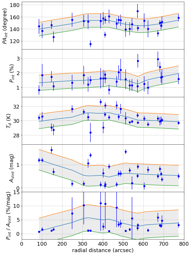
In order to examine the change in the polarization parameters in response to other crucial parameters in the star forming region, we have plotted radial distance (with respect to central coordinates of NGC 1893) versus , , , , and as shown in Figure 14. Here, is the intrinsic total extinction of stars with distance greater than 3 kpc after correcting for a mean foreground extinction of 0.97 mag. is the dust temperature and is the intrinsic polarization efficiency. To make the trends in the plot more clear, we over plot Figure 14 with curves drawn using the locally weighted scattered smoothing (LOWESS) algorithm (Cleveland 1979) from package in python. We use a ‘frac’ parameter of 0.5 to draw the LOWESS curves over all the panels. The corresponding 1- regions (green) bounded by the (orange) and (green) lines are also shown in all the plots.
From Figure 14, the magnetic field orientation, based on the majority values of , is found to be rather uniform without a significant change in the intra cluster medium of NGC 1893 region. The shows a constant trend up to 500, and afterwards it exhibits a scattered distribution. Dust temperature is tending to increase up to 500, and thereafter it decreases. shows a decreasing trend up to 400, and thereafter it remains nearly constant. The intrinsic polarization efficiency, , exhibits an increasing trend up to 400, and thereafter it shows a scattered distribution. Except for and , all parameters show a clear change within the region spread over 400 – 500 in NGC 1893. This is where the two nebulae Sim 129 and Sim 130 are forming due to radiative driven implosion by the UV radiation emanating from the O/B- type stars (Maheswar et al. 2007; Sharma et al. 2007). Changes in various parameters are found to be happening in the area lying between two concentric circles of radii 400″and 500″as shown in Figure 13 (Left). We note here that both tips of Sim 129 and 130, and the shell-like structure surrounding the cluster centre, seem to be formed as a consequence of swept material out of expanding ionization and shock fronts from the O/B type stars formed near the cluster centre.
5 Discussion
From the broken power-law fit and Bayesian analyses of – / (see Figures 4 and 5 and Section 4.1) we show that polarization efficiency (/) exhibits a constant trend as a function of extinction () up to threshold extinction value 0.9 mag with a power-law index of 0 (see, Table 3). This constant trend implies all the dust grains are aligned uniformly, and they polarize the stellar light up to the same degree at all the dust layers located up to 0.9 mag . For 0.9 mag, polarization efficiency declines steeply with 94% highest density interval of indexes ranging from to (see Figure 6 (Top)), indicating poorly aligned dust grains. A number of studies have probed the variation of as a function of towards several dark clouds like Taurus and Rho Ophiuchus molecular cloud complexes using near-infrared observations. Majority of these studies find a drop in as a function of with a typical power law index close to 0.5 (Tamura et al. 1987; Gerakines et al. 1995; Whittet et al. 2008; Chapman et al. 2011; Cashman & Clemens 2014, eg.,). Some studies (Goodman et al. 1995, eg.,) find a constant versus trend, which in terms of versus will follow a steeply decreasing trend, indicating poor dust grain alignment at relatively higher opacities. Arce et al. 1998 have found a linear and flat trends in their versus for the stars lying behind the diffuse and dense regions of Taurus, respectively. However, their data in terms of versus , will follow similar trends that we observed in this work. Similarly, Jones et al. 2014 while studying the variation of fractional polarization per unit optical depth () versus towards a selection of starless cores using NIR and submm observations also find a change in the power-law from 0.5 to 1 at 20 mag which is again similar to our trends. Another study carried out by Wang et al. 2017 showed that broken power-law prevails towards IC 5146 molecular cloud and evidenced a better dust grain alignment at relatively denser regions of the cloud with mag in comparison to the poorly aligned dust grains in the low-density region with 2.25 mag. This result is in contrast to our result of efficiently aligned dust grains in the diffuse ISM and poorly aligned Perseus-arm dust.
From the broken power-law fit and Bayesian analysis of – / as presented in section 4.2, it is seen that the rate of polarization decreases steeply as a function of distance up to a threshold distance of 2 kpc with a relation , thereafter decreases but with a shallower rate with . We found that similar power-law indices have been found by the data on distance versus rate of extinction, versus plot as shown in Figure 15. The data up to 2 kpc follow the relation , while beyond 2 kpc they exhibit . Therefore, the observed trends in the rate of extinction could be reflecting on the rate of polarization because both the quantities, extinction and polarization, are related. However, there exist a difference in the indices of the relations and for stars with > 2 kpc. This implies that although the dust extinction increases abruptly beyond 2 kpc, the amount of polarization does not increase in the same proportion. We suggest that the rate of polarization plot reveals whether the dust grains are distributed in a uniform or non-uniform manner as a function of distance. To confirm this, we have plotted distancei+1 versus differential extinction () in Figure 16, which essentially reveals a constant and scattered distribution of corresponding to uniform and non-uniform dust distributions before and after 2 kpc, respectively.


Based on the analyses – /, – /, and the differential plots, we propose that there exist two dust populations: (i) the foreground dust distributed between local Solar neighbourhood and Perseus arm and is – located up to 2 kpc and characterized by < 1 mag, and (ii) the Perseus arm dust (Perseus-dust) could be part of the Perseus spiral arm in the direction of NGC 1893 and is – distributed beyond 2 kpc and characterized by >1 mag. Foreground dust is found to be uniformly distributed and efficiently aligned to the same degree at all distances to polarize the stellar light efficiently, as clear from the flat distribution in versus plot. In contrast, Persues-dust seems to be non-uniform and not efficient enough to produce the polarization, as clear from the steeply decreasing trend in versus . Therefore, rate of polarization plot reveals about the distribution of dust, whereas the polarization efficiency plot sheds a light on dust grain alignment efficiency. We suggest that the observed differences in the polarization efficiency of the foreground and Perseus-dust are not due to the complex magnetic fields (but because of the differences in the dust distribution and their respective polarization efficiencies) as the magnetic field is found to be uniform across the entire line of sight to NGC 1893.
Although Perseus-dust seems to be non-uniform and poorly aligned, we assume that it infers the intra-cluster medium properties with a proper treatment of foreground subtraction and excluding stars with distance less than 3 kpc as well as lower SN ratio of intrinsic polarization (see Section 4.4). From Figure 14, we notice that , and parameters tend to increase up to 400 – 500 distance from the cluster centre, but the total dust extinction, , decreases up to 400 – 500 distance. at the same time tends to follow a constant trend up to 500. But interestingly, the magnetic field orientation in the cluster region, as inferred by , is found to be nearly constant at all the radial distances. This implies that the increasing trend seen in is not because of spatial variation in and of a constant trend in . Instead, it is most likely caused by an increase in the high energy stellar radiation emanating from the O/B type stars at the cluster center. Two emission nebulae Sim 129 and 130 are formed by the photoevaporation of the pre-existing clouds as a consequence of advancing ionization and shock fronts along with high energy UV photons and stellar winds originating from the O/B-type stars at the center of NGC 1893 cluster (Maheswar et al. 2007; Sharma et al. 2007, see,). It is also possible that a number of newly formed pre-main-sequence stars around these nebulae could also act as secondary sources of radiation in the vicinity of Sim 129 and 130 so as to alter the dust grain alignment.
Such an increase in the amount of radiation towards the two nebulae can also increase the dust temperature . This would result in a better alignment of the dust grains in accordance with the RAT mechanism (Tram et al. 2021). Consequently, this in turn would be resulting in a higher polarization efficiency () towards the two nebulae. Therefore, increase in the amount of radiation could be the plausible reason behind the observed increase in the two parameters , and close to the two emission nebulae in the region distributed between 400 – 500 as represented with two concentric circles in Figure 13 (Left).
We further performed a power-law fit to the versus data to quantify the existence of any positive correlation. As shown in Figure 17, the data exhibits a positive power-law index of 0.66 indicating slow increase in as a function of increase in . To confirm this correlation, we perform the spearman rank-order correlation test using the module in Python. The spearman test gives two outputs: correlation coefficient (r) and probability for an uncorrelated system of datasets (p-value), which are given to be 0.139 and 0.48, respectively. The small positive r-value and statistically insignificant p-value (as p > 0.05) indicates a very weak correlation between and .
Nevertheless, within a range, 29.5 – 31 K, of , the is seen to exhibit a scattered distribution. Within this range of temperatures, some dust grains show relatively higher values ( > 2.3 %) probably due to better alignment by RAT mechanism.
To confirm this, we have examined offset angle () between the magnetic field and the radiation field emanating from two O/B-type stars (HD 242935 and BD +33 1025 that are located at the center of the NGC 1893 cluster) for three stars whose values are higher than 2.3%. The angles are found to be 63, 80, and 68 and in the order of increasing level of . According to Lazarian & Hoang 2021, for >45 the fraction of dust grains driven to high J-attaractor points increase significantly due to weaker rotational disruption and relatively strong RAT, thereby resulting in a higher fraction of polarization (). Therefore, three stars with exhibit relatively higher could be due to enhanced RAT mechanism.

6 summary and conclusions
The main aim of this paper is to investigate whether polarization observations from a distant target enable us to reveal the dust properties and magnetic field orientation within the target of interest. For this purpose, we have studied the variation of interstellar polarization as a function of extinction and distance towards the direction of NGC 1893. We have utilized the newly acquired -band polarization data from ARIES IMaging POLarimeter (AIMPOL) plus the already published -band polarization data (Eswaraiah et al. 2011). In addition, we also utilize distances from Bailer-Jones et al. 2021 and extinction data from Green et al. 2019. We have analysed two key plots (i) polarization efficiency () as a function of extinction () and (ii) rate of polarization () as a function of distance () by employing fitting (i) broken power-law and (ii) Bayesian analysis on both of the plots.
The following are the main conclusions of our study:
- •
The analyses on extinction () versus polarization efficiency () plot reveals a flat trend with a power-law index of 0 up to the threshold extinction, , of 1 mag. For 1 mag, exhibits a steeply decreasing trend with a power-law index ranging from 1.2 to 0.7.
- •
The analyses on distance () versus rate of polarization () suggest that declines steeply with an index of 0.8 up to the threshold distance, , of 1.5 kpc and beyond which the index is found to be 0.6 indicating same declining rate of polarization but with a lesser degree.
- •
Based on the analyses of – and – , we suggest that there exist two dust populations: (1) foreground dust characterized by 1 mag and distributed up to 2 kpc distance, and (2) Perseus-arm dust (Perseus dust) characterized by 1 mag and distributed beyond 2 kpc.
- •
The relations – and – reveal two different clues about the dust grain properties: the former is about dust grain alignment efficiency and the latter is on the distribution of dust.
- •
We find that foreground dust is uniformly distributed and efficiently aligned, whereas the Perseus-dust is non-uniformly distributed and poorly aligned.
- •
After correcting for foreground polarization, we have derived the intrinsic polarization parameters ( and ) and other parameters such as intrinsic extinction (), dust temperature (), and intrinsic polarization efficiency ().
- •
The magnetic field orientation within the star forming region is found to be almost constant, and is not too different from that in the foreground medium.
- •
We notice an increasing trend in , and towards the two nebulae Sim 129 and Sim 130, which we attribute to the increase in the stellar radiation emanating from the O/B-type stars located near the cluster centre of NGC 1893 or to the pre-main-sequence stars in the vicinity of the two nebulae which can act as secondary sources of radiation.
- •
and shows a very weak correlation, however a fewer data points show relatively higher polarization could be due to RAT mechanism.
In order to strengthen our statements, we plan to perform similar analyses using the polarization, extinction, and distance data towards other stellar clusters that are situated towards the direction of, but lying close to, NGC 1893.
Acknowledgements
We thank the referee for constructive suggestions which have improved the content and flow of this paper. C.E. acknowledges the financial support from grant RJF/2020/000071 as a part of Ramanujan Fellowship awarded by Science and Engineering Research Board (SERB), Department of Science and Technology (DST), Govt. of India. C.E. and B.N thank Prem Prakash and Belinda Damian for their help in programming and analyses. This work is done as part of the MS thesis project at Indian Institute of Science Education and Research (IISER) Tirupati.
Data Availability
The partial data is given in Table 1 and the complete dataset can be accessed online in the Harvard Dataverse using the following link: {https://dataverse.harvard.edu/privateurl.xhtml?token=76d51b62-b334-4289-aa3c-34a265634266}.
References
- Amôres et al. (2021) Amôres E. B., et al., 2021, MNRAS, 508, 1788
- Andersson & Potter (2005) Andersson B., Potter S., 2005, Monthly Notices of the Royal Astronomical Society, 356, 1088
- Andersson et al. (2011) Andersson B., Pintado O., Potter S., Straižys V., Charcos-Llorens M., 2011, Astronomy & Astrophysics, 534, A19
- Andersson et al. (2015) Andersson B., Lazarian A., Vaillancourt J. E., 2015, Annual Review of Astronomy and Astrophysics, 53, 501
- Arce et al. (1998) Arce H. G., Goodman A. A., Bastien P., Manset N., Sumner M., 1998, The Astrophysical Journal Letters, 499, L93
- Bailer-Jones et al. (2021) Bailer-Jones C. A. L., Rybizki J., Fouesneau M., Demleitner M., Andrae R., 2021, VizieR Online Data Catalog, p. I/352
- Baug et al. (2020) Baug T., et al., 2020, ApJ, 890, 44
- Bessell & Brett (1988) Bessell M. S., Brett J. M., 1988, PASP, 100, 1134
- Cantat-Gaudin et al. (2019) Cantat-Gaudin T., et al., 2019, Astronomy & Astrophysics, 624, A126
- Cardelli et al. (1989) Cardelli J. A., Clayton G. C., Mathis J. S., 1989, in Allamandola L. J., Tielens A. G. G. M., eds, Vol. 135, Interstellar Dust. pp 5–10
- Cashman & Clemens (2014) Cashman L. R., Clemens D., 2014, The Astrophysical Journal, 793, 126
- Chapman et al. (2011) Chapman N. L., Goldsmith P. F., Pineda J. L., Clemens D., Li D., Krčo M., 2011, The Astrophysical Journal, 741, 21
- Chen et al. (2019) Chen B., et al., 2019, Monthly Notices of the Royal Astronomical Society, 483, 4277
- Cleveland (1979) Cleveland W. S., 1979, Journal of the American Statistical Association, 74, 829
- Cutri et al. (2003) Cutri R. M., et al., 2003, VizieR Online Data Catalog, 2246, 0
- Davis Jr & Greenstein (1951) Davis Jr L., Greenstein J. L., 1951, The Astrophysical Journal, 114, 206
- Dolginov & Mytrophanov (1976) Dolginov A., Mytrophanov I., 1976, Astrophysics and Space Science, 43, 291
- Dougherty et al. (1994) Dougherty S. M., Waters L. B. F. M., Burki G., Cote J., Cramer N., van Kerkwijk M. H., Taylor A. R., 1994, A&A, 290, 609
- Draine & Weingartner (1996) Draine B. T., Weingartner J. C., 1996, ApJ, 470, 551
- Draine & Weingartner (1997) Draine B., Weingartner J. C., 1997, The Astrophysical Journal, 480, 633
- Ducourant et al. (2017) Ducourant C., et al., 2017, Astronomy & Astrophysics, 597, A90
- Eswaraiah et al. (2011) Eswaraiah C., Pandey A. K., Maheswar G., Medhi B. J., Pandey J. C., Ojha D. K., Chen W. P., 2011, MNRAS, 411, 1418
- Eswaraiah et al. (2012) Eswaraiah C., Pandey A. K., Maheswar G., Chen W. P., Ojha D. K., Chandola H. C., 2012, MNRAS, 419, 2587
- Eswaraiah et al. (2013) Eswaraiah C., Maheswar G., Pandey A. K., Jose J., Ramaprakash A. N., Bhatt H. C., 2013, A&A, 556, A65
- Eswaraiah et al. (2019) Eswaraiah C., et al., 2019, The Astrophysical Journal, 875, 64
- Franco et al. (2010) Franco G. A., Alves F. d. O., Girart J. M., 2010, The Astrophysical Journal, 723, 146
- Gaze & Shajn (1952) Gaze V., Shajn G., 1952, Izvestiya Ordena Trudovogo Krasnogo Znameni Krymskoj Astrofizicheskoj Observatorii, 9, 52
- Gerakines et al. (1995) Gerakines P., Whittet D., Lazarian A., 1995, The Astrophysical Journal, 455, L171
- Goodman et al. (1992) Goodman A. A., Jones T. J., Lada E. A., Myers P. C., 1992, The Astrophysical Journal, 399, 108
- Goodman et al. (1995) Goodman A. A., Jones T. J., Lada E. A., Myers P. C., 1995, The Astrophysical Journal, 448, 748
- Green et al. (2015) Green G. M., et al., 2015, ApJ, 810, 25
- Green et al. (2018) Green G. M., et al., 2018, MNRAS, 478, 651
- Green et al. (2019) Green G. M., Schlafly E., Zucker C., Speagle J. S., Finkbeiner D., 2019, ApJ, 887, 93
- Hall (1949) Hall J. S., 1949, Science, 109, 166
- Heiles (2000) Heiles C., 2000, AJ, 119, 923
- Hernández et al. (2005) Hernández J., Calvet N., Hartmann L., Briceño C., Sicilia-Aguilar A., Berlind P., 2005, AJ, 129, 856
- Hiltner (1949a) Hiltner W., 1949a, The Astrophysical Journal, 109, 471
- Hiltner (1949b) Hiltner W., 1949b, Science, 109, 165
- Jones et al. (2014) Jones T. J., Bagley M., Krejny M., Andersson B.-G., Bastien P., 2014, The Astronomical Journal, 149, 31
- Jones et al. (2015) Jones T. J., Bagley M., Krejny M., Andersson B. G., Bastien P., 2015, AJ, 149, 31
- Kharchenko et al. (2005) Kharchenko N. V., Piskunov A. E., Röser S., Schilbach E., Scholz R. D., 2005, A&A, 440, 403
- Krone-Martins et al. (2010) Krone-Martins A., Soubiran C., Ducourant C., Teixeira R., Le Campion J., 2010, Astronomy & Astrophysics, 516, A3
- Kumar et al. (2014) Kumar B., Pandey S., Eswaraiah C., Gorosabel J., 2014, Monthly Notices of the Royal Astronomical Society, 442, 2
- Kumar et al. (2019) Kumar B., et al., 2019, MNRAS, 488, 3089
- Lazarian (2007) Lazarian A., 2007, Journal of Quantitative Spectroscopy and Radiative Transfer, 106, 225
- Lazarian & Hoang (2007) Lazarian A., Hoang T., 2007, MNRAS, 378, 910
- Lazarian & Hoang (2021) Lazarian A., Hoang T., 2021, ApJ, 908, 12
- Lee & Draine (1985) Lee H. M., Draine B. T., 1985, ApJ, 290, 211
- Lee et al. (2018) Lee C., Eswaraiah C., Chen W.-P., Pandey A., 2018, The Astronomical Journal, 156, 115
- Maheswar et al. (2007) Maheswar G., Sharma S., Biman J. M., Pandey A. K., Bhatt H. C., 2007, MNRAS, 379, 1237
- Marco & Negueruela (2002) Marco A., Negueruela I., 2002, A&A, 393, 195
- Massey et al. (1995) Massey P., Johnson K. E., Degioia-Eastwood K., 1995, ApJ, 454, 151
- Melchior & Goulding (2018) Melchior P., Goulding A. D., 2018, Astronomy and computing, 25, 183
- Meyer et al. (1997) Meyer M. R., Calvet N., Hillenbrand L. A., 1997, AJ, 114, 288
- Pandey et al. (2014) Pandey A. K., Samal M. R., Yadav R. K., Richichi A., Lata S., Pandey J. C., Ojha D. K., Chen W. P., 2014, New Astron., 29, 18
- Pattle et al. (2019) Pattle K., et al., 2019, ApJ, 880, 27
- Planck Collaboration et al. (2016a) Planck Collaboration et al., 2016a, A&A, 594, A1
- Planck Collaboration et al. (2016b) Planck Collaboration et al., 2016b, A&A, 594, A8
- Quinn (2012) Quinn J. L., 2012, A&A, 538, A65
- Rautela et al. (2004) Rautela B. S., Joshi G. C., Pandey J. C., 2004, Bulletin of the Astronomical Society of India, 32, 159
- Rice (1945) Rice S. O., 1945, Bell System Technical Journal, 24, 46
- Salvatier et al. (2016) Salvatier J., Wieckia T. V., Fonnesbeck C., 2016, PyMC3: Python probabilistic programming framework (ascl:1610.016)
- Savage & Mathis (1979) Savage B. D., Mathis J. S., 1979, ARA&A, 17, 73
- Schmidt et al. (1992) Schmidt G. D., Elston R., Lupie O. L., 1992, AJ, 104, 1563
- Schnee et al. (2005) Schnee S. L., Ridge N. A., Goodman A. A., Li J. G., 2005, ApJ, 634, 442
- Serkowski et al. (1975) Serkowski K., Mathewson D. S., Ford V. L., 1975, ApJ, 196, 261
- Sharma et al. (2007) Sharma S., Pandey A. K., Ojha D. K., Chen W. P., Ghosh S. K., Bhatt B. C., Maheswar G., Sagar R., 2007, MNRAS, 380, 1141
- Simmons & Stewart (1985) Simmons J. F. L., Stewart B. G., 1985, A&A, 142, 100
- Tamura et al. (1987) Tamura M., Nagata T., Sato S., Tanaka M., 1987, Monthly Notices of the Royal Astronomical Society, 224, 413
- Tram et al. (2021) Tram L. N., Hoang T., Lee H., Santos F. P., Soam A., Lesaffre P., Gusdorf A., Reach W. T., 2021, ApJ, 906, 115
- Van Leeuwen (2007) Van Leeuwen F., 2007, A&A, 474, 653
- Van de Schoot et al. (2021) Van de Schoot R., et al., 2021, Nature Reviews Methods Primers, 1, 1
- Wang et al. (2017) Wang J.-W., Lai S.-P., Eswaraiah C., Clemens D. P., Chen W.-P., Pandey A. K., 2017, ApJ, 849, 157
- Wang et al. (2019) Wang J.-W., et al., 2019, ApJ, 876, 42
- Wardle & Kronberg (1974) Wardle J. F. C., Kronberg P. P., 1974, ApJ, 194, 249
- Whittet (2018) Whittet D. C., 2018, Dust in the galactic environment. CRC press
- Whittet et al. (2008) Whittet D., Hough J., Lazarian A., Hoang T., 2008, The Astrophysical Journal, 674, 304
Appendix A Bayesian analyses
Bayesian analysis is a method of statistical inference, where the available knowledge about parameters in a statistical model is updated with the information in the observed data. The background knowledge is expressed as a prior distribution and combined with observational data in the form of a likelihood function to determine the posterior distribution (Van de Schoot et al. 2021). The most general form of Bayesian inference is:
| (8) | |||||
| (9) |
where is the observed data and represents the model parameters. The posterior describes the probability of the model parameters matching the given data. The evidence is the probability of obtaining the data, which mainly serves as a normalization factor for the posterior. The prior serves as the initial guessing probability of the model parameters based on our prior knowledge. The likelihood describes how likely it is for a given model parameter set to match the observed data.
We already know from previous studies that the probability density function (PDF) of fractional polarization () follows a Rician distribution (Rice 1945; Wardle & Kronberg 1974; Simmons & Stewart 1985; Quinn 2012). Similarly, to determine the exact PDF distributions followed by and we use the package in python. It compares the distributions of and with 26 continuos distributions available in , a module in python, to find the distribution which can fit the and data best. ranks the 26 candidate distributions from best to worst based on their Residual Sum of Squares (RSS) values. As a result, the best fit distributions with the lowest values of RSS are selected. Hence, we find that follow a Student’s T distribution, and has PDF of the form:
| (10) |
where and are the observed and real values of , and is the uncertainty in any observed value of . is the gamma function, and is the degrees of freedom of the Student’s T distribution. Similarly, is found to follow a Rician distribution with the PDF given by:
| (11) |
where and are the observed and real values of and is the uncertainty in any observed value of . is the zeroth order modified Bessel function. The likelihood functions and , respectively for and , can be defined as:
| (12) | |||||
| (13) |
Here represents the measurement of in equation 12 and in equation 13 respectively. To perform the fit to the two plots using Bayesian method, we assume the following broken power-law model for – :
| (14) |
Here , , and are the free model parameters. is the real value of , is , and is the at which break occurs in – . Similarly, for – , we assume a broken power-law similar to equation 14, where , , and are replaced with , and, i.e, the at which the break occurs in – respectively.
For each relation, we define uniform priors within reasonable limits based on the best-fit parameters and their uncertainties from broken power laws (see Section 3.1 and Table 2).
The following are the priors:
(a) For – :
| (15) |
(b) For – :
| (16) |
For the above two plots, Bayesian modelling is performed using a Python package called PyMC3 (Salvatier et al. 2016) via Markov Chain Monte-Carlo (MCMC) method using the Metropolis-Hastings sampling algorithm. The 95%, 68%, and 50% confidence regions (CRs) predicted by the posterior distribution for each of the two plots are shown in Figure 5. From the figures, it is seen that the majority of the data fall well within 95% CR predicted by the posterior. The 94% highest density intervals (HDI) of each parameter are plotted to represent the data lying within uncertainties. The posterior PDF of the parameters derived from the Bayesian modelling is given in Figure 6. The parameters constrained through the Bayesian analyses are reasonably more accurate than those obtained from the broken power-law alone. The constrained results from Bayesian analyses are listed in Table 3.
To determine whether the broken power-law Bayesian model better represent the data over single-power-law Bayesian model, we perform the leave one out () cross-validation using module in Python. cross validation estimates the expected log pointwise predictive density (elpdloo) values for the broken-power law and single-power law bayesian models using the Pareto-smoothed importance sampling (PSIS) procedure. The standard error in elpdloo and the effective number of parameters are also estimated for both models. then compares the broken power-law and single power-law models based on the standard errors in elpdloo values and ranks the models from best to worst. For both – and – , ranked the broken power-law as a better model over the single power-law.