Distributional neural networks for electricity price forecasting
Abstract
We present a novel approach to probabilistic electricity price forecasting which utilizes distributional neural networks. The model structure is based on a deep neural network that contains a so-called probability layer. The network’s output is a parametric distribution with 2 (normal) or 4 (Johnson’s SU) parameters. In a forecasting study involving day-ahead electricity prices in the German market, our approach significantly outperforms state-of-the-art benchmarks, including LASSO-estimated regressions and deep neural networks combined with Quantile Regression Averaging. The obtained results not only emphasize the importance of higher moments when modeling volatile electricity prices, but also – given that probabilistic forecasting is the essence of risk management – provide important implications for managing portfolios in the power sector.
Keywords:
distributional neural network , probabilistic forecasting , quantile regression , lasso , electricity prices , Johnson’s SU distribution1 Introduction and motivation
Trading in competitive markets requires precise probabilistic forecasts. Therefore, the attention of researchers and practitioners is shifting recently from point to probabilistic forecasting methods. It is not different in electricity markets since the liberalization starting in 1990s. The point electricity price forecasting (EPF) literature is very broad, and the topic is well-researched (Weron 2014). However, these models can be used in probabilistic forecasting only to a limited extent, as they mostly predict only the expected price, rarely quantiles or other characteristics. A proper risk optimization that is compulsory in the very volatile and uncertain electricity markets can only be carried out using methods that provide a broader view, such as e.g. distributional forecasting. It did not go unnoticed to researchers (Nowotarski and Weron 2018; Petropoulos et al. 2022), however the literature on probabilistic EPF is much scarcer than the one on point EPF.
We propose a probabilistic EPF approach based on distributional neural networks. More specifically, we consider a ‘vanilla’ deep neural network (DNN), i.e., a multi-layer perceptron in which the information propagates only forward. We utilize the TensorFlow (Abadi et al. 2015) and Keras (Chollet et al. 2015) frameworks, and let the output layer be a parametric distribution with 2 or 4 parameters (Salinas et al. 2020; Barnes and Barnes 2021; Barnes et al. 2021). The difference to a standard network providing point forecasts is only in the output layer. Thus, if we have already built a neural network model for point forecasting, it is very easy to convert it to a distributional one. Even though the method is not new (Nix and Weigend 1994; Williams 1996), it has not attracted much attention. To the best of our knowledge, the only existing distributional networks in the energy forecasting literature use mixtures of normal distributions obtained using complex structures comprising convolutional neural networks (CNN) and gated recurrent units (GRU) (Afrasiabi et al. 2020) or recurrent neural networks (RNN) (Mashlakov et al. 2021; Brusaferri et al. 2020). The distributional deep neural network (DDNN) proposed in this paper is far less complex than the CNNs, GRUs and RNNs, easier to interpret and computationally less demanding.
Neural network-based models are popular and have been shown to achieve good predictive accuracy in the fields of point EPF (Keles et al. 2016; Lago et al. 2021), load forecasting – both point (Yang et al. 2019) and quantile (Zhou et al. 2022) as well as quantile wind power forecasting (He and Zhang 2020). However, despite the relative simplicity of moving from point to probabilistic forecasting using the TensorFlow framework, it has not been utilized in EPF yet.
The performance of the model is evaluated using a rolling window forecasting study with the day-ahead electricity prices in Germany. The DDNN is benchmarked against naive bootstrapping and two well performing point EPF approaches (Lago et al. 2021): a lasso estimated autoregression (LEAR) and a DNN, both combined with quantile regression averaging (QRA) for converting point predictions into probabilistic ones.
The major contributions of the manuscript are as follows:
- 1.
It is the first work to consider the DDNN and one of the first to consider probabilistic neural networks in electricity price forecasting.
- 2.
The proposed method is very simple compared to the existing neural network solutions. As we show in this paper, the generalization from a point to a distributional DNN requires almost no effort.
- 3.
If needed, point forecasts can be easily derived from the predicted distribution.
- 4.
It is the first in EPF and one of the first studies to use the Johnson’s SU (Johnson 1949) distribution in probabilistic forecasting (Mori 2021).
- 5.
It is a fully automatic forecasting method that may be used with other markets and data. The code is open-source.
- 6.
The obtained forecasts are interpretable in terms of distribution’s characteristics, and the results provide evidence of the importance of higher moments in EPF.
- 7.
The aggregation schemes for probabilistic forecasts proposed in the paper yield robust predictions that significantly outperform the state-of-the-art benchmarks in terms of the continuous ranked probability score (CRPS).
Finally, given that probabilistic forecasting is the essence of risk management, our study provides power market participants with a new, significantly more accurate tool for assessing risks related to trading power portfolios.
The remainder of this manuscript is structured as follows. Section 2 introduces the reader to the concept of distributional artificial neural networks. Section 3 provides an overview of the market and data used in the application study. The models, including the DDNN and the hyperparameter tuning, are described in Section 4. The application study together with the results are presented in Section 5. The paper is concluded with a discussion of the main findings in Section 6.
1.1 Probabilistic forecasting literature
The probabilistic EPF literature is not as rich as the one considering point forecasts, what can be deducted from the reviews of Nowotarski and Weron 2018, Ziel and Steinert 2018 and Hong et al. 2020. Researchers consider mainly the day-ahead market, which is the main electricity spot trading place. However in recent years the research focused on other markets as well, e.g. the intraday (Uniejewski et al. 2019; Narajewski and Ziel 2020a; Narajewski and Ziel 2020b; Oksuz and Ugurlu 2019; Janke and Steinke 2019) and balancing markets (Kraft et al. 2020; Browell and Gilbert 2022; Janczura and Wójcik 2022). Two widely used and efficient model estimation methods in point EPF are lasso (Ziel 2016; Ziel and Weron 2018; Uniejewski et al. 2019; Narajewski and Ziel 2020a) of Tibshirani 1996 and artificial neural networks (Dudek 2016; Oksuz and Ugurlu 2019; Zhou et al. 2019; Luo and Weng 2019; Zahid et al. 2019; Lago et al. 2021). A substantial stream of new EPF research considers hybrid models (Jahangir et al. 2019; Zhang et al. 2020; Oreshkin et al. 2021; Olivares et al. 2022), however, as Lago et al. 2021 conclude, they often avoid proper comparisons to well-established methods. The probabilistic EPF comprises mostly of quantile regression (Maciejowska et al. 2016; Marcjasz et al. 2020a; Maciejowska 2020), bootstrapping (Efron 1979) of point forecast residuals (Wan et al. 2013; Ziel and Steinert 2018; Narajewski and Ziel 2022), and of RNNs (Mashlakov et al. 2021; Brusaferri et al. 2020). We follow the recommendations of Lago et al. 2021 and compare our model against the very competitive lasso estimated autoregressive (LEAR) and a point deep neural network. These are point forecasting models, thus we apply quantile regression averaging on them. Other methods of obtaining probabilistic forecasts, such as bootstrap, could be considered as well, but we refrain from that for the sake of simplicity. A vast amount of literature concerns also forecast combinations in the electricity markets (Hubicka et al. 2018; Serafin et al. 2019; Karabiber and Xydis 2019), however due to the complexity of the probabilistic forecast aggregation as pointed out by Berrisch and Ziel 2022, we limit ourselves only to two simple averaging schemes with equal weights that allow to stabilize the neural network predictions.
2 The distributional deep neural network (DDNN) model
We assume that the reader is familiar with and understands the concept of the (feed-forward) deep neural networks (DNN). In this section, we briefly recall the definition and the mathematics behind it to underline the difference between the DNN with point and probabilistic output layers.
2.1 Architecture
Let be the input matrix with denoting the number of features and the number of observations. Further, let be the output matrix of th hidden layer, and be the corresponding hidden-layer weights and bias where is the number of neurons in th hidden layer with and thus . Additionally, denote the th activation function. Then, for we have
| (1) |
Now, we got to the point where the DNN with point and probabilistic output layers differ. That is to say, in the standard DNN we calculate the output , where is the number of modelled features. Formally,
| (2) |
are the values returned by the network. Such DNN is optimized given the true observation matrix with respect to point losses, e.g. the mean squared error (MSE) or mean absolute error (MAE). In the case of the DDNN, the parameter layer consists of distribution parameters for each of the modelled features. It is however computed in the same manner as in equation (2). The final output is made by creating a -dimensional matrix of the assumed distributions . The network is then optimized given the true observation matrix with respect to probabilistic losses, e.g. by maximizing the likelihood for a parametric distribution or by minimizing the continuous ranked probability score (CRPS).
Figure 1 provides an example with hidden layers and this setting we use in the remainder of the manuscript.
The number of neurons in the hidden layers is arbitrary, but the same for both DNNs in order to underline the difference between the point and probabilistic networks. We see clearly that the input and hidden layers are identical for both DNNs and only the output part differs.
As a final remark of the subsection, we discuss the multivariate output which consists of multiple features and the possible probabilistic distributions. Namely, we allow in the definition for output features, and in our setting they are all hours of the electricity prices of the following day. This can be done as all the day-ahead electricity prices are published at once, and therefore they can share the input regressor set. In other applications this is rather not the case, however such a multivariate setting may still be preserved if one considers similar time series to be forecasted that may benefit from common regressors.
The probabilistic output layer may consist of nearly any implemented probabilistic distribution. Based on application, these can be, e.g., binomial or Poisson if we deal with a discrete problem, gamma or beta if we deal with a continuous problem, but supported only on the positive line, or normal, or Johnson’s SU if supported on the whole real line. As the electricity prices may be both positive and negative, we use in our study the two-parametric normal and four-parametric Johnson’s SU distributions.
2.2 Regularization
The danger of overfitting the model can be tackled in the DDNN similarly as in the standard one. One could use regularization, a dropout layer or early stopping. We use all of these in our forecasting study, however we approach the regularization of the parameter layer differently.
The DNN design allows for regularization of every hidden layer , its weights , and bias . Applying it to the DNN we get the following loss with regularization
| (3) | ||||
where represents the norm. One can flexibly choose between the types of regularization, use both or none, and choose to regularize only some part of the network, e.g., only layer and weights. The parameters are subject to hyperparameter tuning. The regularization of the DDNN may be done in the same way as described in Eq. (3), however, we could also regularize each of the distributional parameters separately as follows
| (4) | ||||
The difference between Eq. (4) and Eq. (3) is the regularization of the last layer. Namely, in Eq. (3) we regularize the whole output layer using the same values, whereas in Eq. (4) each parameter is regularized using its own values. The colour arrows in Figure 1(b) denote separate kernel regularization for each of the distributions’ parameters. The reason to use such a differentiation is the possibility to use different amount of inputs’ information for each distribution parameter, what was already observed in the literature (Narajewski and Ziel 2020b).
3 The data
The goal in the empirical case study is forecasting day-ahead electricity prices in Germany. This section familiarizes the reader with the utilized data, especially the input features and the forecasting objective. The electricity markets in Europe consist of derivative, spot and balancing parts (Viehmann 2017). The most important is the spot market, particularly the day-ahead auction. It takes place once a day at noon where all products of the following day are traded in a uniform price auction (Weron and Ziel 2019). In the majority of countries , however in some cases like the UK it is . As all hours of the following day are traded at once, all of them are based on the same set of information. Therefore, in our study we model all the prices using exactly the same input features, what supports the multivariate output of the DDNN presented in Section 2.
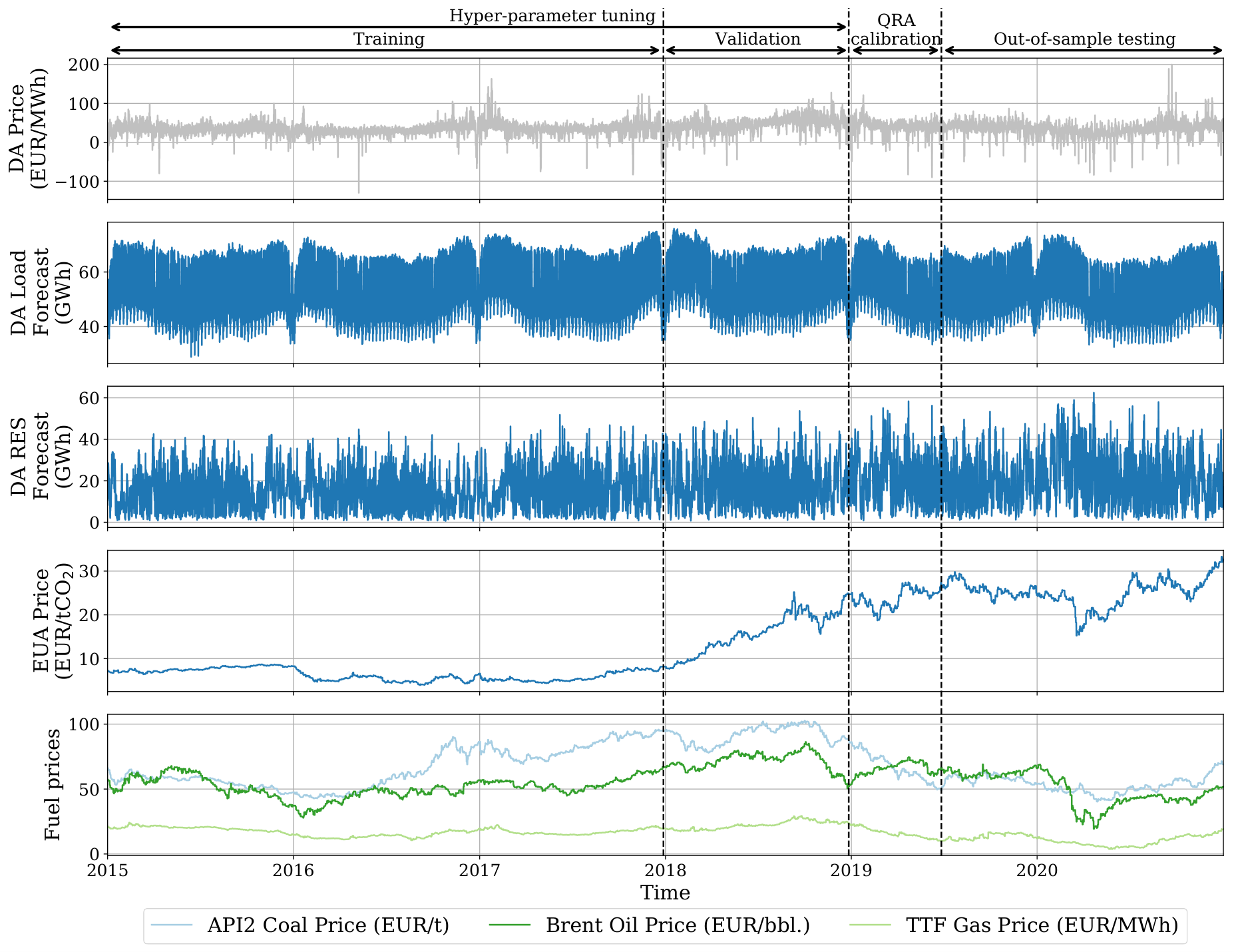
The considered dataset spans six years of hourly observations from 01.01.2015 to 31.12.2020. The study uses a rolling window what mimics the daily business in practice and is a standard procedure in the EPF literature (Weron 2014; Weron and Ziel 2019). The initial in-sample period spans the date range from 01.01.2015 to 26.12.2018 which consists of observations. For the purpose of hyperparameter tuning, we split it additionally to training and validation sets. The out-of-sample period starts on 27.12.2018, and ends on 31.12.2020, however the first 182 observations are used to obtain the QRA forecasts and thus are excluded from the analysis. Therefore, the final out-of-sample test set for probabilistic predictions uses 554 days of data. The models are retrained every day using the most recent observations and the hyperparameters obtained in the tuning that is run on initial in-sample dataset.
Figure 2 shows plots of the considered features together with the dates and study stages mentioned above. The data contains the day-ahead (DA) electricity prices, DA load forecasts, DA renewable energy sources (RES) forecasts, EU emission allowance prices and fuel: coal, oil and natural gas prices. The RES forecast is a sum of wind offshore, wind onshore and solar generation day-ahead forecasts. The DA prices and load forecasts exhibit strong daily, weekly and annual seasonality. Thus, we model each hour of the day separately within a single neural network and also utilize the weekday dummies. We do not construct any regressor explaining the annual behavior as it is well described by the load data. On the other hand, the RES forecasts exhibit only daily and annual seasonality and the EUA and fuel prices are random-walk type processes. These conclusions might not be easy to derive based on Figure 2, however see Ziel and Weron 2018, Sgarlato and Ziel 2022 and Billé et al. 2022 for more insights.
Figure 3 presents histograms of prices for selected hours.
Additionally, we fit there normal and Johnson’s SU distributions and plot their densities. Both distributions belong to the location-scale family. The normal distribution is a well-known two-parametric distribution with being the location and the scale parameters. The Johnson’s SU distribution was first investigated by Johnson 1949 as a transformation of the normal distribution. It is a four-parametric distribution with being the location, the scale, the skewness and the tail-weight parameters. So far, it has not found application with distributional neural networks. However, it is often used in the context of energy commodities (Patra 2021; Gianfreda and Bunn 2018; Abramova and Bunn 2020). Based on Figure 3 we suspect that the Johnson’s SU is more suitable for modeling the electricity prices than the normal. We observe heavy tails and skewness what cannot be explained by the normal distribution. Thus, in the forecasting study we use both distributions to emphasize the gain that comes from using the more flexible distribution.
4 Models and estimation
4.1 Input features
Let us recall that we forecast the day-ahead prices on day , i.e. . The following input features are available for all considered models:
- 1.
Past day-ahead prices of the previous three days and one week ago, i.e. , , , and .
- 2.
Day-ahead forecasts of the total load for day , i.e. , as well as the past values of the previous day and one week ago, i.e. , and .
- 3.
Day-ahead forecasts of renewable energy sources (RES) for day , i.e. , as well as the past values of the previous day, i.e. .
- 4.
EU emission allowance most recent closing price, i.e. .
- 5.
Fuels most recent closing prices, i.e. , , and .
- 6.
Weekday dummies, i.e. for .
Let us note that the forecasting exercise is performed on day before the day-ahead auction. That is to say, we possess only the information available at around 11:30 CET on day . The considered input does not violate this assumption, and therefore we use e.g. lag for the EUA and fuels prices.
4.2 Probabilistic neural network
The probabilistic NN model uses the DDNN described in Section 2. The model consists of 2 hidden layers, output distributions, and various number of input features. The output distributions are assumed to be either normal or Johnson’s SU and each of them defines a separate model. We regularize the model through input feature selection, dropout layer and regularization of the hidden layers and weights. All these are subject to hyperparameter tuning. Additionally, we tune the activation functions, the number of neurons, and the learning rate. The detailed list of hyperparameters and the process is described in Section 4.2.1.
The model is built and estimated using the TensorFlow (Abadi et al. 2015) and Keras (Chollet et al. 2015) frameworks. The hyperparameter optimization is performed with the help of Optuna (Akiba et al. 2019) package, 4 times for result stability reasons, each time consisting of 2048 iterations. We report the results for each of the 4 optimized hyperparameter sets, as well as for 3 different ensembles of the four distributions, as described in Section 5. The model consists naturally also of components that are not tuned in the hyperparameter optimization. That is to say, the model uses additionally an input normalization, negative loglikehood as the loss function, Adam optimizing algorithm, and early stopping callback with patience of 50 epochs. The batch size is fixed to 32, and the maximum number of epochs to 1500. For the rolling prediction, the dataframe was shuffled and was left out for validation.
Probabilistic neural networks are denoted in the later parts of the paper using DDNN-{distribution}-{run} scheme, where {distribution} is either Normal (or N) or JSU and {run} is either a number from 1 to 4 (corresponding to the individual hyperparameter sets), or an indicator of the ensemble of the four: pEns for the vertical average or qEns for the horizontal averaging. See Section 4.2.1 for the description of different schemes. Note, that when the choice of the distribution is obvious, as in Fig. 5, the {distribution} term may be missing in the model acronym.
4.2.1 Hyperparameter tuning for neural network models
The neural network models (both point and distributional) underwent the hyperparameter optimization considering below hyperparameters and their potential values:
- 1.
Indicator for inclusion of input features described in Section 4.1 (14 hyperparameters).
- 2.
Dropout layer – whether to use the dropout layer after the input layer, and if yes at what rate. The rate parameter is drawn from (0, 1) interval (up to 2 hyperparameters – the rate is not optimized if dropout layer is not present in the model).
- 3.
Number of neurons in the hidden layers. The values are chosen from integers from [16, 1024] interval (1 hyperparameter per layer).
- 4.
Activation functions used in each of the hidden layers. The possible functions are: elu, relu, sigmoid, softmax, softplus, and tanh (1 hyperparameter per layer).
- 5.
regularization for hidden layers – whether to use the regularization on the hidden layers and their weights and if yes at what rate. The rate is drawn from interval on a log-scale (up to 2 hyperparameters per layer – inclusion of for the layer and the rate).
- 6.
regularization for distribution layer – separate for each of the distribution parameters, where for normal and for Johnson’s SU distributions – whether to use the regularization and if yes at what rate (a total of hyperparameters; rates identical to the hidden layer regularization).
- 7.
Learning rate for the Adam algorithm chosen from the interval on a log-scale (1 hyperparameter).
The process consists of 2048 iterations of the optimization algorithm which are performed in a hybrid batch-rolling approach. Having the first four years (1456 days) at disposal, we split them into training data (the first 1092 days) and validation data (the last 364 days). Note, that the first day of the out-of-sample test window is the day after the end of the hyperparameter validation data, as illustrated on Figure 2 (i.e., there is no data contamination). The hybrid approach is needed to balance two opposing factors. On one hand, a batch estimation (using a single estimation on NN weights) would be less computationally demanding (we would only have 1 neural network trained for every considered hyperparameter set), however the results of such an experiment are very volatile. The best hyperparameter set chosen using the accuracy metric of only a single run would not – in general – guarantee a good predictive performance. On the other hand, a rolling setting identical to the one used later (i.e., with a daily recalibration) would be infeasible to compute (as it would take roughly 364 times longer than for batch approach – we would have 364 neural networks trained for every hyperparameter set). The hybrid approach we have chosen uses 13 recalibrations of neural network models with batches of 28 days estimated using each of the nets. Training data is rolled by 28 days after each step.
As mentioned earlier, to counteract the local behavior of the hyperparameter optimizer, we repeat the process four times for each of the neural networks. We observe that the predictive performance across the separate hyperparameter sets is not consistent, however the simple aggregation schemes described below provide results consistently better than any of the inputs.
The first of the aggregation schemes is a mixture distribution, which corresponds to averaging the distributions vertically. However, having two distributions with disjoint pdfs (e.g., two copies of the same distributions significantly shifted), the resulting mixture will be very wide, and might have a “gap” in the middle. A more robust alternative is considered, which utilizes horizontal (quantile) averaging – i.e., a quantile of an ensemble is computed as an arithmetic mean of the same quantiles from all distributions considered. Such an aggregation in an edge case described earlier would result in an unimodal ensemble distribution, which is much sharper than the vertically averaged one.
4.3 Benchmarks
4.3.1 The naive model
The first and the simplest benchmark model that we consider is the well-known and widely utilized (Weron 2014; Ziel and Weron 2018) naive model. It requires no parameter tuning. Its formula is as follows
| (5) |
In other words, the naive model uses the prices of yesterday to forecast the prices on Tuesday, Wednesday, Thursday and Friday, and the last week’s prices on Monday, Saturday and Sunday. The price distributions are obtained using the bootstrap method which was first proposed by Efron 1979. We receive the distributions by adding the in-sample bootstrapped errors to the forecasted expected price
| (6) |
where are drawn with replacement in-sample residuals for day , i.e., we sample from the set of for .
4.3.2 The LEAR model combined with QRA
The first of the models that use the structure presented in Section 4.1 is LEAR point forecasting model that uses Quantile Regression Averaging (QRA) to generate probabilistic forecasts. The LEAR model utilizes the LASSO regularization (Tibshirani 1996). Such an approach eliminates the need for an additional input selection, as the algorithm itself indirectly chooses the most relevant inputs. The regularization parameter (the sole hyperparameter of the LEAR model) is obtained using 7-fold cross validation and a grid of 100 values automatically chosen by a least angle regression (LARS) based estimator. The LEAR approach encompasses a forecast averaging scheme proposed by Lago et al. 2021 – four independent forecasts are generated for each hour (based on 56, 84, 1092 and 1456 day rolling calibration windows) and the final output is their simple average. Such an approach allows for a balance of the ability to adapt to rapidly-changing market conditions (thanks to the shorter calibration windows) with robustness coming from the use of long windows. It was shown to provide forecasts that – on average – are on par or better than all of the comprising forecasts considered separately (Lago et al. 2021).
There are two ways of using a set of four separate forecasts or an ensemble: one that uses the whole information directly (i.e., the separate forecasts), which we will denote QRA (Quantile Regression Averaging) and QRM (Quantile Regression committee Machine) that uses the ensemble of the point predictions (Marcjasz et al. 2020b).
Aside from the input data, the QRA and QRM approaches are identical – both use quantile regression with 182 day rolling calibration window to produce the forecast for each of the 99 percentiles, which approximate the predictive distribution relatively well.
The LEAR models’ results are denoted by LEAR-{CAL} for the point forecast estimated using {CAL} calibration days (e.g., LEAR-1456 for the longest calibration window), LEAR-Ens for an hour-by-hour average of all 4 point forecasts and LEAR-QRA and -QRM for the probabilistic forecasts.
4.3.3 The DNN model combined with QRA
The second set of benchmarks utilizes a point neural network model. It differs from the probabilistic counterpart only in the output construction in the network and hyperparameters corresponding to the missing distribution layer (see Sections 2, 4.2 and Figure 1). The rest of the model setting remains unchanged: DNN model has the same inputs, the same hyperparameter selection and uses the same calibration window lengths and training and validation splits. The loss function for the network is MAE, whereas DDNN uses log-likelihood.
Similarly to the DDNN, for the (point) DNN we also derive four independently-trained hyperparameter sets. This allows us to i) measure the robustness of the predictions and ii) apply two quantile-regression based methods (QRA and QRM), similarly as for the LEAR point predictions, also using a 182 day rolling calibration window.
The results are marked with DNN-n for the point forecasts (where or Ens) and DNN-QRA and DNN-QRM, respectively for percentile forecasts obtained using quantile regression on the four separate point forecasts and their ensemble.
5 Empirical results
Many earlier works show that forecast averaging is often key to achieving accurate predictions. Here, we also aggregate multiple forecast runs to improve the result accuracy and robustness. However, considering probabilistic forecasts instead of the point ones significantly increases the complexity of the aggregation schemes that can be applied. As the detailed discussion is out of scope of this paper, we opted to include only the simple aggregations, based on the equally-weighted averaging or distribution mixing.
On the probabilistic forecasts side, we have four hyperparameter sets chosen in four separate hyperparameter optimization runs for both the normal and JSU DDNNs. We report the errors of each of them separately, as well as the result of two aggregation schemes: an equally-weighted mixture of the four resulting distributions (vertical aggregation) or a mean of values for a given quantile (horizontal aggregation).
5.1 Evaluation
While the paper focuses on probabilistic forecasting, we are also interested in the accuracy of the point forecasts. The latter can be easily derived from the probabilistic ones. Following the best practices of Weron and Ziel 2019, we report two point-oriented metrics: the mean absolute error(MAE; we use median statistic from the probabilistic methodologies for this metric) and root mean squared error (RMSE; we use mean statistic).
When it comes to the probabilistic forecasts, we use the CRPS, or rather its approximation – an average pinball score across 99 percentiles.(Gneiting 2011; Hong et al. 2016):
| (7) | ||||
where is the forecast of the -th quantile of the price .
Additionally for each hour of the day, we perform the Kupiec test (Kupiec 1995) for unconditional coverage for 50% and 90% prediction intervals (PIs). For the CRPS, we aggregate the score across all forecasted hours, whereas for the Kupiec test, we provide the number of hours which passed the Kupiec test.
Lastly, we use the Diebold-Mariano (DM) test that measures the statistical significance of the difference between the accuracy of the forecasts of two models (here, we use and to discern between them) (Uniejewski et al. 2019; Muniain and Ziel 2020; Sgarlato and Ziel 2022). Let us denote the vector of errors (here, the CRPS scores) of model for day as . Then, the multivariate loss differential series
| (8) |
defines the difference of the norm of loss vectors. For each pair of models, we compute the -value of two one-sided DM tests – one with the null hypothesis , which corresponds to the outperformance of model forecasts by those of model and the second with the reverse null hypothesis , complementary to the first one. We use the CRPS as the loss function.
5.2 Results
| MAE | RMSE | CRPS | Kupiec 50% | Kupiec 90% | |
| LEAR-Ens | 4.372 | 6.375 | - | - | - |
| DNN-Ens | 3.610 | 5.850 | - | - | - |
| naive | 9.336 | 14.358 | 3.585 | 21 | 23 |
| LEAR-QRA | 4.161 | 6.676 | 1.575 | 10 | 8 |
| LEAR-QRM | 4.285 | 6.788 | 1.662 | 6 | 3 |
| DNN-QRA | 3.668 | 5.845 | 1.399 | 6 | 10 |
| DNN-QRM | 3.670 | 5.821 | 1.412 | 9 | 8 |
| DDNN-N-pEns | 3.663 | 5.962 | 1.351 | 2 | 6 |
| DDNN-N-qEns | 3.670 | 5.962 | 1.348 | 13 | 20 |
| DDNN-JSU-pEns | 3.542 | 6.146 | 1.304 | 1 | 4 |
| DDNN-JSU-qEns | 3.564 | 6.174 | 1.299 | 14 | 13 |
In terms of the CRPS scores, as can be seen in Figure 5 and Table 1, the LEAR-based methods are significantly worse than the neural network-based approaches. However, the performance of the latter is not robust – run-to-run, the CRPS scores differ by as much as 10%. As discussed in Section 5.3, this is not known ex-ante, therefore an aggregation scheme is needed. After ensembling, regardless of the aggregation scheme applied (vertical, horizontal with mean, horizontal with median), we see similar performance. The normally-distributed networks yield a CRPS of ca. 1.35, whereas JSU ones – 1.30, i.e., ca. 3-4% better than the normal. DNN-QR methods can be placed between the probabilistic DDNN ensembles and the individual runs.
As shown in Table 1, the neural network-based models are better than LEAR-based ones also for the point forecasts. Interestingly, the ensemble of DNN forecasts has the third lowest error – both in terms of MAE and RMSE. The best model according to MAE is DDNN-JSU-pEns, followed by its -qEns counterpart – the two models with the best CRPS score. However, these models are worse w.r.t. the RMSE than all other NN-based models. On the other hand, we see the lowest RMSE for DNN-QR based methods, closesly followed by the DNN-Ens model. The DDNNs are ca 2% (normal) and 7% (JSU) worse. There are only minor differences between the vertical and horizontal aggregation schemes.
Additionally, we performed the Kupiec test for unconditional coverage with 5% significance level for 50% and 90% prediction intervals. From what can be seen in Table 1, QRA seems to perform better than QRM – for both the LEAR and point DNN models. However, the QR-based approahces pass the Kupiec test for at most 10 hours of the day. The probabilistic DDNNs, on the other hand show mixed performance. The p-Ens forecasts are worse than most other methods, while q-Ens are better than QR-based predictions. As the p-Ens models sport the CRPS scores similar to the q-Ens ones, the latter are a much better choice, especially when chosen with a more robust median quantile instead of mean. Note, however, that the worst overall method (Naive benchmark) provides the best coverage for both 50 and 90% PIs.
Lastly, the results of the DM test are visualized in Figure 6. We can observe that DDNN-JSU-qEns is the best model overall, with forecasts significantly better than from any other model (represented by a column with all cells green or yellow). Secondly, the DDNN-N-qEns is also significantly better than both other aggregation schemes. Lastly, QRA models (both LEAR and DNN ones) produce significantly better forecasts than their QRM counterparts.
5.3 The need for multiple hyperparameter sets
Even though the hyperparameter optimization uses a repeated neural network training procedure to mimic the rolling calibration window setting used later for the evaluation, the optimal sets obtained using independent hyperparameter trials differ significantly. Moreover, all the optimal sets have a similar, i.e. within 2% difference, in-sample error metric – what is not reflected in the out-of-sample error obtained using this set. Here, the differences are much more prominent, up to 10%. The locality of the hyperparameter optimization is clearly visible in the optimal sets chosen in independent trials, despite most of the trials being stalled after around 1000 iterations. Figure 7 shows choice frequency of the considered input features (i.e., the number of hyperparameter sets that uses a particular input variable), described in Section 4.1. All 3 considered neural network models are quite consistent when selecting the inputs. The most important ones are the prices of the previous day and two days ago, the current DA forecasts of load and RES, the previous day’s DA forecasts of RES and the recent gas price. The least important are the further lags of prices and load forecast.
Besides the differences in the inputs chosen, hidden layer sizes are the most prominent, especially for the probabilistic networks. They found optima in both the larger and smaller networks, as shown in Table 2. For example, one of the probabilistic neural networks that used the JSU distribution uses 565 and 962 neurons in the hidden layers (amounting to over 540,000 weights just between the two hidden layers), whereas other had 940 and 58 (over 54,000 weights) or 123 and 668 (over 82,000 weights). Moreover, even the activation functions chosen were not unanimous, but softplus seems to be the best for the first hidden layer. We also observe that the dropout is almost never chosen, similarly to the regularization of the network weights.
| DNN | DDNN-N | DDNN-JSU | |||||||||||
| Run | 1 | 2 | 3 | 4 | 1 | 2 | 3 | 4 | 1 | 2 | 3 | 4 | |
| Layer 1 | Activation | softplus | softplus | softplus | softplus | softplus | softplus | softplus | softplus | softplus | elu | softplus | softplus |
| Neurons | 906 | 912 | 979 | 965 | 948 | 266 | 542 | 110 | 565 | 940 | 243 | 123 | |
| Layer 2 | Activation | softplus | softplus | relu | elu | elu | relu | softplus | relu | relu | elu | elu | elu |
| Neurons | 901 | 619 | 767 | 448 | 554 | 883 | 641 | 823 | 962 | 58 | 895 | 668 | |
To conclude, we observe that there is a need for repeating the hyperparameter optimization process. Despite the robust optimization setting, the end results are vastly different – both in terms of the parameters chosen, and the out-of-sample error metrics. A form of the forecast combination is crucial for the outperformance of QR-based methods.
6 Conclusions
The paper proposes an application of distributional neural networks to probabilistic day-ahead electricity price forecasting and a simple, yet well-performing aggregation scheme for the distributional neural networks that stabilizes the predictions. Since probabilistic forecasting is the essence of risk management – Value-at-Risk (VaR) is nothing else but a quantile forecast – our study provides important implications for managing portfolios in the power sector.
Comparing the results with the literature approaches, we observe a strong performance of the neural networks – both the probabilistic forecasts from the proposed methods and from quantile regression applied to their point counterparts are significantly more accurate than the statistical-based combination of LEAR and quantile regression. The added complexity of the neural network having to model the distribution of the data, rather than just their expected values, proves effective, especially when the limitations incurred by the distribution choice are not too severe.
Interestingly, the benefit of using distributional neural networks is visible also when mean absolute errors of the median (50th percentile) forecasts are considered. The DDNN-JSU-Ens approach is the only one that outperforms the ensemble of point NNs in this regard.
Acknowledgments
This research was partially supported by the Ministry of Science and Higher Education (MNiSW, Poland) through Diamond Grant No. 0219/DIA/2019/48 (to G.M.) and the National Science Center (NCN, Poland) through grant No. 2018/30/A/HS4/00444 (to R.W. and F.Z.).
References
- Abadi et al. (2015) Abadi, M., Agarwal, A., Barham, P., et al., 2015. TensorFlow: Large-Scale Machine Learning on Heterogeneous Systems. URL: https://www.tensorflow.org/. software available from tensorflow.org.
- Abramova and Bunn (2020) Abramova, E., Bunn, D., 2020. Forecasting the intra-day spread densities of electricity prices. Energies 13, 687.
- Afrasiabi et al. (2020) Afrasiabi, M., Mohammadi, M., Rastegar, M., Stankovic, L., Afrasiabi, S., Khazaei, M., 2020. Deep-based conditional probability density function forecasting of residential loads. IEEE Transactions on Smart Grid 11, 3646–3657.
- Akiba et al. (2019) Akiba, T., Sano, S., Yanase, T., Ohta, T., Koyama, M., 2019. Optuna: A next-generation hyperparameter optimization framework, in: Proceedings of the 25th ACM SIGKDD international conference on knowledge discovery & data mining, pp. 2623–2631.
- Barnes and Barnes (2021) Barnes, E.A., Barnes, R.J., 2021. Controlled abstention neural networks for identifying skillful predictions for classification problems. Journal of Advances in Modeling Earth Systems 13, e2021MS002573.
- Barnes et al. (2021) Barnes, E.A., Barnes, R.J., Gordillo, N., 2021. Adding uncertainty to neural network regression tasks in the geosciences arXiv:2109.07250.
- Berrisch and Ziel (2022) Berrisch, J., Ziel, F., 2022. CRPS Learning. Journal of Econometrics doi:10.1016/j.jeconom.2021.11.008.
- Billé et al. (2022) Billé, A.G., Gianfreda, A., Del Grosso, F., Ravazzolo, F., 2022. Forecasting electricity prices with expert, linear, and nonlinear models. International Journal of Forecasting doi:10.1016/j.ijforecast.2022.01.003.
- Browell and Gilbert (2022) Browell, J., Gilbert, C., 2022. Predicting electricity imbalance prices and volumes: Capabilities and opportunities. Energies 15.
- Brusaferri et al. (2020) Brusaferri, A., Matteucci, M., Ramin, D., Spinelli, S., Vitali, A., 2020. Probabilistic day-ahead energy price forecast by a Mixture Density Recurrent Neural Network, in: 2020 7th International Conference on Control, Decision and Information Technologies (CoDIT), pp. 523–528.
- Chollet et al. (2015) Chollet, F., et al., 2015. Keras. https://keras.io.
- Dudek (2016) Dudek, G., 2016. Multilayer perceptron for GEFCom2014 probabilistic electricity price forecasting. International Journal of Forecasting 32, 1057–1060.
- Efron (1979) Efron, B., 1979. Bootstrap Methods: Another Look at the Jackknife. The Annals of Statistics , 1–26.
- Gianfreda and Bunn (2018) Gianfreda, A., Bunn, D., 2018. A stochastic latent moment model for electricity price formation. Operations Research 66, 1189–1203.
- Gneiting (2011) Gneiting, T., 2011. Quantiles as optimal point forecasts. International Journal of Forecasting 27, 197–207.
- He and Zhang (2020) He, Y., Zhang, W., 2020. Probability density forecasting of wind power based on multi-core parallel quantile regression neural network. Knowledge-Based Systems 209, 106431.
- Hong et al. (2016) Hong, T., Pinson, P., Fan, S., Zareipour, H., Troccoli, A., Hyndman, R.J., 2016. Probabilistic energy forecasting: Global energy forecasting competition 2014 and beyond. International Journal of Forecasting 32, 896–913.
- Hong et al. (2020) Hong, T., Pinson, P., Wang, Y., Weron, R., Yang, D., Zareipour, H., 2020. Energy forecasting: A review and outlook. IEEE Open Access Journal of Power and Energy 7, 376–388.
- Hubicka et al. (2018) Hubicka, K., Marcjasz, G., Weron, R., 2018. A note on averaging day-ahead electricity price forecasts across calibration windows. IEEE Transactions on Sustainable Energy 10, 321–323.
- Jahangir et al. (2019) Jahangir, H., Tayarani, H., Baghali, S., Ahmadian, A., Elkamel, A., Golkar, M.A., Castilla, M., 2019. A novel electricity price forecasting approach based on dimension reduction strategy and rough artificial neural networks. IEEE Transactions on Industrial Informatics 16, 2369–2381.
- Janczura and Wójcik (2022) Janczura, J., Wójcik, E., 2022. Dynamic short-term risk management strategies for the choice of electricity market based on probabilistic forecasts of profit and risk measures. the German and the Polish market case study. Energy Economics 110, 106015.
- Janke and Steinke (2019) Janke, T., Steinke, F., 2019. Forecasting the price distribution of continuous intraday electricity trading. Energies 12, 4262.
- Johnson (1949) Johnson, N.L., 1949. Systems of frequency curves generated by methods of translation. Biometrika 36, 149–176.
- Karabiber and Xydis (2019) Karabiber, O.A., Xydis, G., 2019. Electricity price forecasting in the Danish day-ahead market using the TBATS, ANN and ARIMA methods. Energies 12, 928.
- Keles et al. (2016) Keles, D., Scelle, J., Paraschiv, F., Fichtner, W., 2016. Extended forecast methods for day-ahead electricity spot prices applying artificial neural networks. Applied Energy 162, 218–230.
- Kraft et al. (2020) Kraft, E., Keles, D., Fichtner, W., 2020. Modeling of frequency containment reserve prices with econometrics and artificial intelligence. Journal of Forecasting 39, 1179–1197.
- Kupiec (1995) Kupiec, P.H., 1995. Techniques for verifying the accuracy of risk measurement models. The Journal of Derivatives 3.
- Lago et al. (2021) Lago, J., Marcjasz, G., De Schutter, B., Weron, R., 2021. Forecasting day-ahead electricity prices: A review of state-of-the-art algorithms, best practices and an open-access benchmark. Applied Energy 293, 116983.
- Luo and Weng (2019) Luo, S., Weng, Y., 2019. A two-stage supervised learning approach for electricity price forecasting by leveraging different data sources. Applied Energy 242, 1497–1512.
- Maciejowska (2020) Maciejowska, K., 2020. Assessing the impact of renewable energy sources on the electricity price level and variability–A quantile regression approach. Energy Economics 85, 104532.
- Maciejowska et al. (2016) Maciejowska, K., Nowotarski, J., Weron, R., 2016. Probabilistic forecasting of electricity spot prices using Factor Quantile Regression Averaging. International Journal of Forecasting 32, 957–965.
- Marcjasz et al. (2020a) Marcjasz, G., Uniejewski, B., Weron, R., 2020a. Probabilistic electricity price forecasting with narx networks: Combine point or probabilistic forecasts? International Journal of Forecasting 36, 466–479.
- Marcjasz et al. (2020b) Marcjasz, G., Uniejewski, B., Weron, R., 2020b. Probabilistic electricity price forecasting with narx networks: Combine point or probabilistic forecasts? International Journal of Forecasting 36, 466–479.
- Mashlakov et al. (2021) Mashlakov, A., Kuronen, T., Lensu, L., Kaarna, A., Honkapuro, S., 2021. Assessing the performance of deep learning models for multivariate probabilistic energy forecasting. Applied Energy 285, 116405.
- Mori (2021) Mori, R., 2021. Off-block time prediction using operators’ prediction history, in: 2021 IEEE/AIAA 40th Digital Avionics Systems Conference (DASC), pp. 1–7.
- Muniain and Ziel (2020) Muniain, P., Ziel, F., 2020. Probabilistic forecasting in day-ahead electricity markets: Simulating peak and off-peak prices. International Journal of Forecasting 36, 1193–1210.
- Narajewski and Ziel (2020a) Narajewski, M., Ziel, F., 2020a. Econometric modelling and forecasting of intraday electricity prices. Journal of Commodity Markets 19, 100107.
- Narajewski and Ziel (2020b) Narajewski, M., Ziel, F., 2020b. Ensemble forecasting for intraday electricity prices: Simulating trajectories. Applied Energy 279, 115801.
- Narajewski and Ziel (2022) Narajewski, M., Ziel, F., 2022. Optimal bidding on hourly and quarter-hourly day-ahead electricity price auctions: trading large volumes of power with market impact and transaction costs. Energy Economics 110, 105974.
- Nix and Weigend (1994) Nix, D., Weigend, A., 1994. Estimating the mean and variance of the target probability distribution, in: Proceedings of 1994 IEEE International Conference on Neural Networks (ICNN’94), pp. 55–60.
- Nowotarski and Weron (2018) Nowotarski, J., Weron, R., 2018. Recent advances in electricity price forecasting: A review of probabilistic forecasting. Renewable and Sustainable Energy Reviews 81, 1548–1568.
- Oksuz and Ugurlu (2019) Oksuz, I., Ugurlu, U., 2019. Neural network based model comparison for intraday electricity price forecasting. Energies 12, 4557.
- Olivares et al. (2022) Olivares, K.G., Challu, C., Marcjasz, G., Weron, R., Dubrawski, A., 2022. Neural basis expansion analysis with exogenous variables: Forecasting electricity prices with NBEATSx. International Journal of Forecasting doi:10.1016/j.ijforecast.2022.03.001.
- Oreshkin et al. (2021) Oreshkin, B.N., Dudek, G., Pełka, P., Turkina, E., 2021. N-beats neural network for mid-term electricity load forecasting. Applied Energy 293, 116918.
- Patra (2021) Patra, S., 2021. Revisiting value-at-risk and expected shortfall in oil markets under structural breaks: The role of fat-tailed distributions. Energy Economics 101, 105452.
- Petropoulos et al. (2022) Petropoulos, F., Apiletti, D., Assimakopoulos, V., et al., 2022. Forecasting: theory and practice. International Journal of Forecasting 38, 705–871.
- Salinas et al. (2020) Salinas, D., Flunkert, V., Gasthaus, J., Januschowski, T., 2020. Deepar: Probabilistic forecasting with autoregressive recurrent networks. International Journal of Forecasting 36, 1181–1191.
- Serafin et al. (2019) Serafin, T., Uniejewski, B., Weron, R., 2019. Averaging predictive distributions across calibration windows for day-ahead electricity price forecasting. Energies 12, 2561.
- Sgarlato and Ziel (2022) Sgarlato, R., Ziel, F., 2022. The role of weather predictions in electricity price forecasting beyond the day-ahead horizon. IEEE Transactions on Power Systems doi:10.1109/TPWRS.2022.3180119.
- Tibshirani (1996) Tibshirani, R., 1996. Regression shrinkage and selection via the lasso. Journal of the Royal Statistical Society: Series B (Methodological) 58, 267–288.
- Uniejewski et al. (2019) Uniejewski, B., Marcjasz, G., Weron, R., 2019. Understanding intraday electricity markets: Variable selection and very short-term price forecasting using LASSO. International Journal of Forecasting 35, 1533–1547.
- Viehmann (2017) Viehmann, J., 2017. State of the German Short-Term Power Market. Zeitschrift für Energiewirtschaft 41, 87–103.
- Wan et al. (2013) Wan, C., Xu, Z., Wang, Y., Dong, Z.Y., Wong, K.P., 2013. A hybrid approach for probabilistic forecasting of electricity price. IEEE Transactions on Smart Grid 5, 463–470.
- Weron (2014) Weron, R., 2014. Electricity price forecasting: A review of the state-of-the-art with a look into the future. International journal of forecasting 30, 1030–1081.
- Weron and Ziel (2019) Weron, R., Ziel, F., 2019. Electricity price forecasting, in: Soytaş, U., Sarı, R. (Eds.), Routledge handbook of energy economics. Routledge, pp. 506–521.
- Williams (1996) Williams, P.M., 1996. Using neural networks to model conditional multivariate densities. Neural Computation 8, 843–854.
- Yang et al. (2019) Yang, A., Li, W., Yang, X., 2019. Short-term electricity load forecasting based on feature selection and least squares support vector machines. Knowledge-Based Systems 163, 159–173.
- Zahid et al. (2019) Zahid, M., Ahmed, F., Javaid, N., Abbasi, R.A., Zainab Kazmi, H.S., Javaid, A., Bilal, M., Akbar, M., Ilahi, M., 2019. Electricity price and load forecasting using enhanced convolutional neural network and enhanced support vector regression in smart grids. Electronics 8, 122.
- Zhang et al. (2020) Zhang, F., Fleyeh, H., Bales, C., 2020. A hybrid model based on bidirectional long short-term memory neural network and Catboost for short-term electricity spot price forecasting. Journal of the Operational Research Society , 1–25.
- Zhou et al. (2019) Zhou, S., Zhou, L., Mao, M., Tai, H.M., Wan, Y., 2019. An optimized heterogeneous structure LSTM network for electricity price forecasting. IEEE Access 7, 108161–108173.
- Zhou et al. (2022) Zhou, X., Wang, J., Wang, H., Lin, J., 2022. Panel semiparametric quantile regression neural network for electricity consumption forecasting. Ecological Informatics 67, 101489.
- Ziel (2016) Ziel, F., 2016. Forecasting electricity spot prices using lasso: On capturing the autoregressive intraday structure. IEEE Transactions on Power Systems 31, 4977–4987.
- Ziel and Steinert (2018) Ziel, F., Steinert, R., 2018. Probabilistic mid-and long-term electricity price forecasting. Renewable and Sustainable Energy Reviews 94, 251–266.
- Ziel and Weron (2018) Ziel, F., Weron, R., 2018. Day-ahead electricity price forecasting with high-dimensional structures: Univariate vs. multivariate modeling frameworks. Energy Economics 70, 396–420.