Note on graph-based BCJ relation for Berends-Giele currents

In BS theory, the Berends-Giele current $\phi(1,2,\dots,n-1|\boldsymbol{\sigma})$, where $\boldsymbol{\sigma}$ is a permutation of $n-1$ elements (which are not necessarily the elements $1$, …, $n-1$), can be recursively defined Mafra:2016ltu by

In the above expression, $s_{12\dots n-1}\equiv(k_{1}+k_{2}+...+k_{n-1})^{2}$, where $k_{i}$ is the momentum of the particle $i$ which satisfies the on-shell condition $k_{i}^{2}=0$. This recursive definition starts with the one-point current $\phi(l|l^{\prime})$ that is defined by

A consequent result of the definition is $\phi(a_{1},\dots,a_{i}|b_{1},\dots,b_{i})=0$ if $\{a_{1},\dots,a_{i}\}\setminus\{b_{1},\dots,b_{i}\}\neq\emptyset$. The $n$-point on-shell partial amplitude $\mathcal{A}(1,2,\dots,n|\boldsymbol{\sigma})$ is obtained by taking the following limit

Berends-Giele currents (2.1) in BS theory satisfy Kleiss-Kuijf (KK) relation Kleiss:1988ne

where $\boldsymbol{\alpha}$, $\boldsymbol{\beta}$ are two ordered sets, and $\boldsymbol{\beta},1,\boldsymbol{\alpha}$ is a permutation of $n-1$ elements. The notation $|\boldsymbol{\beta}|$ stands for the number of elements in the ordered set $\boldsymbol{\beta}$, and $\boldsymbol{\beta}^{T}$ denotes the inverse permutation of $\boldsymbol{\beta}$. For two ordered sets $\boldsymbol{A}$ and $\boldsymbol{B}$, $\boldsymbol{A}\shuffle\boldsymbol{B}$ denotes the set of all shuffle permutations, which are obtained by merging $\boldsymbol{A}$ and $\boldsymbol{B}$ together with keeping the relative order of elements in each ordered set. For example, $\{2,4\}\shuffle\{3,5\}$ involves the following permutations

When the ordered set $\boldsymbol{\alpha}$ in eq. (2.6) is empty, KK relation turns into the reflection relation

For given two ordered sets $\boldsymbol{\alpha}\in\mathcal{P}(\{i_{1},..,i_{l}\})$ and $\boldsymbol{\beta}\in\mathcal{P}(\{1,2,...,n-1\}\setminus\{i_{1},..,i_{l}\})$ where $i_{1},..,i_{l}\in\{1,2,...,n-1\}$ and $\mathcal{P}(\{i_{1},..,i_{l}\})$ denotes the set of all permutations of $i_{1},..,i_{l}$, the Berends-Giele currents satisfy the following identity

which is essentially equivalent to the KK relation (2.6).

As pointed in Wu:2021bcy, Berends-Giele currents (2.1) satisfy so-called graph-based BCJ relation whose on-shell version was first proposed for YM amplitudes Hou:2018bwm. To show this relation, we introduce permutations $\boldsymbol{\sigma}$ for a given connected tree graph $\mathcal{T}$ and a given node $a\in\mathcal{T}$ as follows: (i). the node $a$ is considered as the leftmost element in $\boldsymbol{\sigma}$, (ii). for any two adjacent elements $x$ and $y$, we have ${\sigma}^{-1}(x)<\sigma^{-1}(y)$ ¹¹ 1 The notation ${\sigma}^{-1}(x)$ denotes the position of the element $x$ in the permutation $\boldsymbol{\sigma}$. In some places, we used $x\prec y$ to stand for ${\sigma}^{-1}(x)<\sigma^{-1}(y)$ for simplicity. if $x$ is nearer to $a$ than $y$, (iii). for subtrees attached to a same node, we shuffle the permutations corresponding to these subtrees together. The collection of all such permutations is denoted by $\mathcal{T}|_{a}$. For example, the set of permutations established by Fig. 1 when the node $1$ is considered as the leftmost element are given by

Having the above definition, we define the following combination of BS currents which are characterized by two connected tree graphs $\mathcal{T}_{\boldsymbol{A}}$ and $\mathcal{T}_{\boldsymbol{B}}$:

where $s_{ac}=(k_{a}+k_{c})^{2}$. On the LHS of the above expression, $x$ is an arbitrarily chosen node in $\mathcal{T}_{\boldsymbol{A}}$, while $\boldsymbol{\sigma}$ is an arbitrary permutation of all elements corresponding to nodes. On the RHS, the first summation is taken over all choices of $c$ in $\mathcal{T}_{\boldsymbol{B}}$. The second and the third summations are taken over permutations established by $\mathcal{T}_{\boldsymbol{A}}$ and $\mathcal{T}_{\boldsymbol{B}}$ when $a$ and $b$ are considered as the leftmost elements, respectively. We further sum over all the shuffle permutations such that $c\prec a$ and associate a factor $s_{ac}$ to a given choice of $c$. The $|ax|$ denotes the distance between $a$ and $x$ (the number of edges between $a$ and $x$). According to this definition, the sign $(-)^{|ax|}$ can be determined as follows: (i). if $a=x$, $(-)^{|ax|}=1$, (ii) for two adjacent nodes $y$ and $z$, $(-)^{|yx|}=-(-)^{|zx|}$. With the combination (2.11), graph-based BCJ relation for BS currents is introduced as

where $\boldsymbol{\sigma}_{i,j}$ ($i<j$) denotes $\{\sigma_{i},\sigma_{i+1},...,\sigma_{j}\}$ for short, the number of nodes in the two graphs $\mathcal{T}_{\boldsymbol{A}}$ and $\mathcal{T}_{\boldsymbol{B}}$ are supposed to be $i$ and $l-i$, respectively ²² 2 In Wu:2021bcy, we have checked the relation up to six-point scattering..

The simplest example is the case in which each of $\mathcal{T}_{\boldsymbol{A}}$ and $\mathcal{T}_{\boldsymbol{B}}$ contains only one node, say $1$ and $2$, respectively. When the Berends-Giele recursion (2.1) for the BS current $\phi(\sigma_{1},\sigma_{2}|2,1)$ is substituted into the LHS of (2.12), we get

which reproduces the RHS of the graph-based BCJ relation (2.12) with $\mathcal{T}_{\boldsymbol{A}}=\{1\}$ and $\mathcal{T}_{\boldsymbol{B}}=\{2\}$.

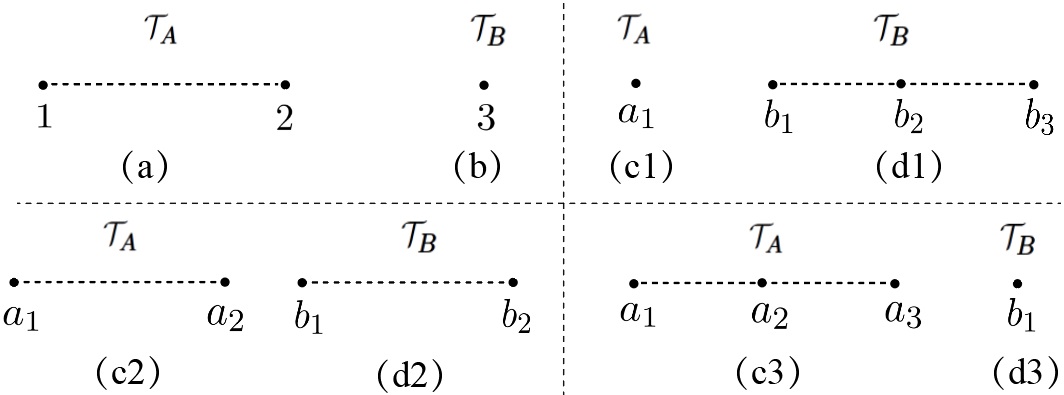
The second example is given by relations for three-point Berends-Giele currents. There are two possible cases corresponding to distinct number of nodes in the two graphs.

Now let us study the example in which $\mathcal{T}_{\boldsymbol{A}}$ corresponds to the star graph Fig. 3 (a), while $\mathcal{T}_{\boldsymbol{B}}$ refers to the single node $5$. Although the relation (2.12) in this case can also be directly verified via Berends-Giele recursion, we illustrate this example in another way, by expanding the combinations corresponding to the start graph in terms of those corresponding to simple chains.

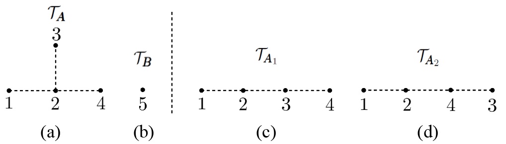
Particularly, the LHS of (2.12) for $\mathcal{T}_{{A}}=\text{Fig.~\ref{Fig:StarGraphExample} (a)}$ and $\mathcal{T}_{{B}}=\text{Fig.~\ref{Fig:StarGraphExample} (b)}$ can be expanded as

where $\boldsymbol{\sigma}$ stands for a permutation with the five external particles, while $\mathcal{T}_{\boldsymbol{A}_{1}}$ and $\mathcal{T}_{\boldsymbol{A}_{2}}$ are the two simple chains, as shown by Fig. 3 (c), (d). This can be easily verified by writing down the permutations and signs corresponding to $\mathcal{T}_{\boldsymbol{A}}$, $\mathcal{T}_{\boldsymbol{A}_{1}}$ and $\mathcal{T}_{\boldsymbol{A}_{2}}$ explicitly

Once $\mathbb{B}^{(1)}(\boldsymbol{\sigma}\,|\,\mathcal{T}_{\boldsymbol{A}_{1}},\mathcal{T}_{\boldsymbol{B}}|_{b})$ and $\mathbb{B}^{(1)}(\boldsymbol{\sigma}\,|\,\mathcal{T}_{\boldsymbol{A}_{2}},\mathcal{T}_{\boldsymbol{B}}|_{b})$, where $\mathcal{T}_{\boldsymbol{A}_{1}}$ and $\mathcal{T}_{\boldsymbol{A}_{2}}$ are the simple chains Fig. 3 (c) and (d) respectively, satisfy the relation (2.12), we have

According to the first line of (3.11), the sum of $\mathbb{B}^{(1)}(\boldsymbol{\sigma}\,|\,\mathcal{T}_{\boldsymbol{A}_{1}},\mathcal{T}_{\boldsymbol{B}}|_{b})$ and $\mathbb{B}^{(1)}(\boldsymbol{\sigma}\,|\,\mathcal{T}_{\boldsymbol{A}_{2}},\mathcal{T}_{\boldsymbol{B}}|_{b})$ precisely reproduces

which is the RHS of (2.12) with $\mathcal{T}_{\boldsymbol{A}}=\text{Fig.~\ref{Fig:StarGraphExample} (a)}$ and $\mathcal{T}_{\boldsymbol{B}}=\text{Fig.~\ref{Fig:StarGraphExample} (b)}$.

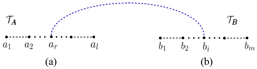
When both $\mathcal{T}_{\boldsymbol{A}}$ and $\mathcal{T}_{\boldsymbol{B}}$ stand for simple chains, as shown by Fig. 4, the LHS of eq. (2.12) are expressed by

where we have written $s_{a_{r},b_{i}}$ by $2k_{a_{r}}\cdot k_{b_{i}}$ explicitly. The permutations $\boldsymbol{\gamma}$ for given $i$, $r$ are defined by

Noting that one can exchange the summations over $i$ and $\boldsymbol{\gamma}$ in eq. (4.1) by collecting the coefficients corresponding to a given $\boldsymbol{\gamma}$ and then summing over all possible permutations. As a result, $\mathbb{B}^{(a_{1})}\left(\boldsymbol{\sigma}\,|\,\mathcal{T}_{\boldsymbol{A}},\mathcal{T}_{\boldsymbol{B}}|_{b_{1}}\right)$ is reexpressed by

where we have summed over all possible $\boldsymbol{\gamma}$ satisfying

Expressing each current in eq. (4.3) by Berends-Giele recursion (2.1), we rewrite eq. (4.3) as

where $n-1=l+m$ is the total number of on-shell particles. One can collect those subcurrents with the same particle contents but distinct permutations together. The contributions of the first term in the above expression can be collected as follows, according to whether $a_{r}\in\boldsymbol{\gamma}_{1,j}$ or $a_{r}\in\boldsymbol{\gamma}_{j+1,n-1}$.

References

- (1) S. Stieberger and T. R. Taylor, New relations for Einstein-Yang-Mills amplitudes, Nucl. Phys. B 913 (2016) 151–162, [arXiv:1606.09616].
- (2) D. Nandan, J. Plefka, O. Schlotterer, and C. Wen, Einstein-Yang-Mills from pure Yang-Mills amplitudes, JHEP 10 (2016) 070, [arXiv:1607.05701].
- (3) O. Schlotterer, Amplitude relations in heterotic string theory and Einstein-Yang-Mills, JHEP 11 (2016) 074, [arXiv:1608.00130].
- (4) C.-H. Fu, Y.-J. Du, R. Huang, and B. Feng, Expansion of Einstein-Yang-Mills Amplitude, JHEP 09 (2017) 021, [arXiv:1702.08158].
- (5) M. Chiodaroli, M. Gunaydin, H. Johansson, and R. Roiban, Explicit Formulae for Yang-Mills-Einstein Amplitudes from the Double Copy, JHEP 07 (2017) 002, [arXiv:1703.00421].
- (6) F. Teng and B. Feng, Expanding Einstein-Yang-Mills by Yang-Mills in CHY frame, JHEP 05 (2017) 075, [arXiv:1703.01269].
- (7) Y.-J. Du, B. Feng, and F. Teng, Expansion of All Multitrace Tree Level EYM Amplitudes, JHEP 12 (2017) 038, [arXiv:1708.04514].
- (8) Y.-J. Du and F. Teng, BCJ numerators from reduced Pfaffian, JHEP 04 (2017) 033, [arXiv:1703.05717].
- (9) Z. Bern, J. J. M. Carrasco, and H. Johansson, New Relations for Gauge-Theory Amplitudes, Phys. Rev. D 78 (2008) 085011, [arXiv:0805.3993].
- (10) Z. Bern, J. J. M. Carrasco, and H. Johansson, Perturbative Quantum Gravity as a Double Copy of Gauge Theory, Phys. Rev. Lett. 105 (2010) 061602, [arXiv:1004.0476].
- (11) V. Del Duca, L. J. Dixon, and F. Maltoni, New color decompositions for gauge amplitudes at tree and loop level, Nucl. Phys. B 571 (2000) 51–70, [hep-ph/9910563].
- (12) L. Hou and Y.-J. Du, A graphic approach to gauge invariance induced identity, JHEP 05 (2019) 012, [arXiv:1811.12653].
- (13) Y.-J. Du and L. Hou, A graphic approach to identities induced from multi-trace Einstein-Yang-Mills amplitudes, JHEP 05 (2020) 008, [arXiv:1910.04014].
- (14) H. Tian, E. Gong, C. Xie, and Y.-J. Du, Evaluating EYM amplitudes in four dimensions by refined graphic expansion, JHEP 04 (2021) 150, [arXiv:2101.02962].
- (15) Z. Bern, T. Dennen, Y.-t. Huang, and M. Kiermaier, Gravity as the Square of Gauge Theory, Phys. Rev. D82 (2010) 065003, [arXiv:1004.0693].
- (16) N. E. J. Bjerrum-Bohr, P. H. Damgaard, T. Sondergaard, and P. Vanhove, The Momentum Kernel of Gauge and Gravity Theories, JHEP 01 (2011) 001, [arXiv:1010.3933].
- (17) Y.-J. Du, B. Feng, and C.-H. Fu, BCJ Relation of Color Scalar Theory and KLT Relation of Gauge Theory, JHEP 08 (2011) 129, [arXiv:1105.3503].
- (18) J. Broedel, O. Schlotterer, and S. Stieberger, Polylogarithms, Multiple Zeta Values and Superstring Amplitudes, Fortsch. Phys. 61 (2013) 812–870, [arXiv:1304.7267].
- (19) F. Cachazo, S. He, and E. Y. Yuan, Scattering equations and Kawai-Lewellen-Tye orthogonality, Phys. Rev. D90 (2014), no. 6 065001, [arXiv:1306.6575].
- (20) F. Cachazo, S. He, and E. Y. Yuan, Scattering of Massless Particles in Arbitrary Dimensions, Phys. Rev. Lett. 113 (2014), no. 17 171601, [arXiv:1307.2199].
- (21) F. Cachazo, S. He, and E. Y. Yuan, Scattering of Massless Particles: Scalars, Gluons and Gravitons, JHEP 07 (2014) 033, [arXiv:1309.0885].
- (22) F. Cachazo, S. He, and E. Y. Yuan, Einstein-Yang-Mills Scattering Amplitudes From Scattering Equations, JHEP 01 (2015) 121, [arXiv:1409.8256].
- (23) C. R. Mafra, Berends-Giele recursion for double-color-ordered amplitudes, JHEP 07 (2016) 080, [arXiv:1603.09731].
- (24) C. R. Mafra and O. Schlotterer, A solution to the nonlinear field equations of ten dimensional supersymmetric Yang-Mills theory, Phys Rev.D 92 (2015) 066001, [arXiv:1501.05562].
- (25) S. Lee, C. R. Mafra, and O. Schlotterer, Non-linear gauge transformations in SYM theory and the BCJ duality, JHEP 03 (2016) 090, [arXiv:1510.08843].
- (26) E. Bridges and C. R. Mafra, Algorithmic construction of SYM multiparticle superfields in the BCJ gauge, JHEP 10 (2019) 022, [arXiv:1906.12252].
- (27) H. Frost, C. R. Mafra, and L. Mason, A Lie bracket for the momentum kernel, arXiv:2012.00519.
- (28) K. Wu and Y.-J. Du, Off-shell extended graphic rule and the expansion of Berends-Giele currents in Yang-Mills theory, JHEP 01 (2021) 162, [arXiv:2109.14462].
- (29) F. A. Berends and W. T. Giele, Recursive Calculations for Processes with n Gluons, Nucl. Phys. B 306 (1988) 759.
- (30) N. E. J. Bjerrum-Bohr, P. H. Damgaard, and P. Vanhove, Minimal Basis for Gauge Theory Amplitudes, Phys. Rev. Lett. 103 (2009) 161602, [arXiv:0907.1425].
- (31) S. Stieberger, Open & Closed vs. Pure Open String Disk Amplitudes, arXiv:0907.2211.
- (32) Y.-X. Chen, Y.-J. Du, and B. Feng, A Proof of the Explicit Minimal-basis Expansion of Tree Amplitudes in Gauge Field Theory, JHEP 02 (2011) 112, [arXiv:1101.0009].
- (33) R. Kleiss and H. Kuijf, Multi - Gluon Cross-sections and Five Jet Production at Hadron Colliders, Nucl. Phys. B 312 (1989) 616–644.
- (34) B. Feng, R. Huang, and Y. Jia, Gauge Amplitude Identities by On-shell Recursion Relation in S-matrix Program, Phys. Lett. B695 (2011) 350–353, [arXiv:1004.3417].
- (35) Q. Ma, Y.-J. Du, and Y.-X. Chen, On Primary Relations at Tree-level in String Theory and Field Theory, JHEP 02 (2012) 061, [arXiv:1109.0685].
- (36) H. Frost, The Algebraic Structure of the KLT Relations for Gauge and Gravity Tree Amplitudes, SIGMA 17 (2021) 101, [arXiv:2111.07257].