Nuclear incompressibility and sound speed in uniform matter and finite nuclei

The NEP, e.g., $E_{\mathrm{sat}}$, $E_{\mathrm{sym}}$, are defined as the coefficients of the series expansion of the energy per particle in SM ($e_{\mathrm{SM}}$) and of the symmetry energy ($e_{\mathrm{sym}}$) as,

where $x=(n-n_{\mathrm{sat}})/3n_{\mathrm{sat}}$, with $n_{\mathrm{sat}}$ being the saturation density of nuclear matter ($n_{\mathrm{sat}}=0.155\pm 0.005$ fm^-3, see for instance Ref. Margueron et al. 2018a). Note that choosing $n_{\mathrm{sat}}$ as the reference density for the parameter $x$, is arbitrary: in Sec. II.2 for instance, we explore another reference density. It should also be noted that in Eq. (7), the symmetry energy is defined as the difference between neutron matter (NM) and SM energies, as $e_{\mathrm{sym}}(n)=e_{\mathrm{NM}}(n)-e_{\mathrm{SM}}(n)$. It can be expanded in terms of $\delta^{2}$ as $e_{\mathrm{sym}}(n)=e_{\mathrm{sym},2}(n)\delta^{2}+e_{\mathrm{NQ}}$, where $e_{\mathrm{sym},2}$ and $e_{\mathrm{NQ}}$ subsume the quadratic and non-quadratic (NQ) contributions respectively.

It was suggested in Ref. Margueron et al. 2018a to consider the series expansion up to order 4 in the density parameter $x$ in order to represent accurately the energy per particle, the pressure and the sound speed of existing models up to about $4n_{\mathrm{sat}}$. We adopt this prescription here as well, even if we do not explore such high densities.

Note that since asymmetric matter is mostly quadratic in $\delta$, as it is expected to be Somasundaram et al. 2021a, Eqs. (6)-(7) could also be written in a more compact way,

where

It should be noted that the above expression of K($\delta)$ is by no means the true isospin dependence of the incompressibility, as it will be discussed below. In particular, it neglects the contribution of the pressure which is different from zero as one gets farther from saturation. It solely represents the second order term in the density expansion of the energy per particle.

From Eq. (9), one could deduce a similar expression for the energy density $\epsilon_{\mathrm{UM}}=(1+3x)e_{\mathrm{UM}}n_{\mathrm{sat}}$ as,

where

with

The $\delta$-dependence of the energy density curvature $K^{\epsilon}(\delta)$ is different from that of the energy per particle curvature $K(\delta)$. Consequences will be discussed in the following, especially for the incompressibility modulus in asymmetric matter. It will be shown that $K^{\epsilon}(\delta)$ do correspond to the isospin dependence of the incompressibility around saturation density, contrarily to K_sym, which is only a parameter useful in the expansion (9)

The general expressions for the pressure (5) and the incompressibility modulus (4) in AM could be expressed in terms of the parameter $x$ as,

Injecting Eq. (9) into the expression for the pressure  (16), we obtain

where $K^{p}=K^{\epsilon}$ and $Q^{p}$ reads

with

Note that in finite nuclei, $|\delta_{A}|<0.3$ and densities are explored from about $2/3n_{\mathrm{sat}}$ up to $n_{\mathrm{sat}}$, which implies $|x_{A}|\lesssim 0.1$. In finite nuclei, we could therefore perform an expansion at the same level in $\delta^{2}$ and in $x$.

The equilibrium density in AM is given by the density for which the mechanical stability is satisfied: $\partial e_{\mathrm{UM}}(x,\delta)/\partial x=0$. From the expression of the pressure (16) truncated at order $x$, one can deduce in AM Piekarewicz and Centelles 2009,

The equilibrium density is a function of the isospin asymmetry parameter $\delta$, and it satisfies the limit $n_{\mathrm{eq}}^{\mathrm{UM}}\rightarrow n_{\mathrm{sat}}$ for $\delta\rightarrow 0$. At order $\delta^{2}$ and $x$, one obtains for the equilibrium density $n_{\mathrm{eq}}^{\mathrm{UM}}$ in asymmetric matter, $n_{\mathrm{eq}}^{\mathrm{UM}}=n_{\mathrm{sat}}[1-3(L_{\mathrm{sym}}/K_{\mathrm{sat}})\delta^{2}]$.

In finite nuclei, the situation is more complex than previously described since: i) the equilibrium density is different from $n_{\mathrm{sat}}$, due to the finite size terms and ii) the density is not uniform allowing for surface contributions to be sizeable. In uniform matter however, only isospin asymmetry contributes to the shift of the equilibrium density from $n_{\mathrm{sat}}$, as shown in Eq. (22). While neglecting the contribution of the finite-size (FS) terms, expression (22) provides a good estimation of the average densities in finite nuclei Papakonstantinou et al. 2013. In the next section, this density is named $n_{\mathrm{cl}}$ in the CLDM and we have $n_{\mathrm{cl}}\approx n_{\mathrm{eq}}^{\mathrm{UM}}$ for large $A$.

The pressure could be decomposed into a SM and an isospin asymmetry terms:

with

We have for instance $P_{\mathrm{sym}}(n_{\mathrm{sat}})=n_{\mathrm{sat}}L_{\mathrm{sym}}/3$, as expected.

Similarly, injecting Eq. (9) into (), one obtains the following expression for the incompressibility modulus

with $K^{k}=K^{p}=K^{\epsilon}$ and $Q^{k}=Q^{p}$, and where the additional coefficient in asymmetric matter reads

with

Remark that while $K(\delta)$ controls the isoscalar and isovector dependence of the curvature of the energy per particle in uniform matter  (9), the incompressibility () itself is driven by the parameter $K^{k}(\delta)$ for $x=0$. The difference between $K(\delta)$ and $K^{k}(\delta)$ reflects the contribution of the pressure, which is non-zero as soon as the density departs from the equilibrium density $n_{\mathrm{eq}}^{\mathrm{UM}}$, see Eq. (4). This contribution is unavoidable, making $K^{k}(\delta)$ the true isospin dependence of the incompressibility Piekarewicz and Centelles 2009. Fixing $n=n_{\mathrm{sat}}$ for instance, the parameter which controls the isospin dependence of the incompressibility is $K^{k}_{\mathrm{sym}}=K_{\mathrm{sym}}+6L_{\mathrm{sym}}$, and not K_sym alone. Considering $L_{\mathrm{sym}}\approx 50$ MeV and $K_{\mathrm{sym}}\approx-100$ MeV d’Etivaux et al. 2019; Sagawa et al. 2019, with a lower limit provided by the unitary limit Tews et al. 2017, the parameter $K^{k}_{\mathrm{sym}}$ is even mostly controlled by $L_{\mathrm{sym}}$, and only moderately by $K_{\mathrm{sym}}$.

In SM the incompressibility modulus can be expressed as a series expansion in $x$ as

and we introduce a new quantity,

which represents the incompressibility modulus of SM for the equilibrium density $n_{\mathrm{eq}}^{\mathrm{UM}}$:

One can show that in AM the incompressibility modulus at the equilibrium density (26) can be expressed as,

In Eq. (32), the isovector term $K_{\mathrm{sym}}^{k}$=$K_{\mathrm{sym}}^{\epsilon}$ (15) depends only on isovector empirical parameters $L_{\mathrm{sym}}$ and $K_{\mathrm{sym}}$, while the isoscalar term only depends on isoscalar NEPs $K_{\mathrm{sat}}$ and $Q_{\mathrm{sat}}$, provided $x_{\mathrm{eq}}^{\mathrm{UM}}$ is known (experimentally for instance). In order to perform comparisons with incompressibilities in nuclei $K_{A}$, it could be relevant to express the incompressibility modulus in AM at equilibrium density $x=x_{\mathrm{eq}}^{\mathrm{UM}}$ as,

where Piekarewicz and Centelles 2009

We choose nine Skyrme models, BSK14Goriely et al. 2007, BSK16Chamel et al. 2008, F0Lesinski et al. 2006, LNS5Cao et al. 2006, RATPRayet et al. 1982, SGIIVan Giai and Sagawa 1981, SKI2Reinhard and Flocard 1995, SKOReinhard et al. 1999, SLy5Chabanat et al. 1998, which NEP are given in Table 1. For these nine interactions, while the parameter $K^{k}_{\mathrm{sym}}$ is positive for actual values of the NEPs, the parameter $K_{\tau}$ controlling the isovector dependence of $K_{\mathrm{eq}}$ is negative since $Q_{\mathrm{sat}}/K_{\mathrm{sat}}\approx-1.5$ from Table 1. Note however that the value of $Q_{\mathrm{sat}}$ has never been measured and its actual value is not necessarily in the range given in Table 1. Aside from the finite size contribution, the ISGMR in finite nuclei is mostly correlated with $K_{\mathrm{eq}}$, whose isospin dependence is given by $K_{\tau}$ Piekarewicz and Centelles 2009. This is the reason why the isovector dependence of the ISGMR across isotopic chains has been correlated with the parameter $K_{\tau}$ Li et al. 2010.

It is clear from the definition of $K_{\tau}$ (34) that here also, a precise experimental determination of $K_{\tau}$ does not necessarily lead to a better value for the NEP $K_{\mathrm{sym}}$, since $K_{\tau}$ is mostly correlated with $L_{\mathrm{sym}}$, which is not precisely known. In order to extract $K_{\mathrm{sym}}$ from experimental investigations, one has to precisely know the values of $L_{\mathrm{sym}}$ and $Q_{\mathrm{sat}}$. Note that with about 10% accuracy Khan et al. 2012; Khan and Margueron 2013; Khan et al. 2013, the NEP $K_{\mathrm{sat}}$ is sufficiently well known in the present case.

An illustration of the different points where the incompressibility has been introduced is shown in Fig. 1. It displays the behavior of the equilibrium density as a function of $\delta$, on the example of the BSk12 functional. The role of the incompressibility at various densities and isospin is also displayed on the figure. It shows that several incompressibilities at various densities are probed when the GMR is measured in a given nuclei. For instance, in addition to the saturation density, their typical mean density is around 0.11 fm^-3 Khan et al. 2012; Khan and Margueron 2013. It should be noted that $K^{k}_{\mathrm{sym}}$ drives the isospin dependence of the incompressibility, independently of the considered density, from $x=0$ (saturation point) to $x=x^{\mathrm{UM}}_{\mathrm{eq}}$ (equilibrium point).

In this section, we explore an alternative representation of the uniform matter properties, where the equilibrium density $n_{\mathrm{eq}}$ is taken, in place of the saturation density $n_{\mathrm{sat}}$. This alternative representation is equivalent to the existing one up to $\delta^{2}$, but generates non-quadratic terms. In the view of constraining uniform matter parameters from measurements of incompressibilities in nuclei, it may be more relevant to consider such a representation: the equilibrium density in uniform matter shall be closer – than the saturation density – to the average one of the nucleus Khan et al. 2012; Khan and Margueron 2013.

In this alternative approach, the associated density parameter is set to be $\tilde{x}=(n-n_{\mathrm{eq}}^{\mathrm{UM}})/(3n_{\mathrm{eq}}^{\mathrm{UM}})$, from which the density $n$ is obtained as $n/n_{\mathrm{eq}}^{\mathrm{UM}}=1+3\tilde{x}$.

The alternative density parameter $\tilde{x}$ can be expressed in term of $x$ as,

Similarly to Eq. (9) one can expand the energy per particle in term of $\tilde{x}$ as

with

It should be noted that K_τ in Eq. (38) corresponds to (34), because it is the incompressibility at the equilibrium density, namely $\tilde{K}(\delta)$=K_eq.

Imposing the equality between the $\delta^{2}$ terms in the series expansions  (9) and (36) orders by orders in $x$, one obtains the following relations,

where $Y_{\mathrm{sat}}$ is the fifth order NEP. Note that these equations are a generalization of Eq. (16) of Ref. Piekarewicz and Centelles 2009 up to the 4^th order, and hence, the above equation for K_τ is the same than the one of the previous subsection.

Eqs. (9) and (36) are identical up to terms in $\delta^{2}$. In Eq. (36) there are however non-quadratic terms, which are small even when $\delta\sim 1$. The contribution of these non-quadratic terms (because of the denominator in Eq. (35)) is even more suppressed by the fact that finite nuclei do not explore large values for $\delta$, since $|\delta_{A}|<0.3$, as previously discussed. So it is possible to use both Eq. (9) or Eq. (36) to describe the energy in finite nuclei.

Expressing the incompressibility modulus in asymmetric matter () as a function of the density parameter $\tilde{x}$:

where we have used $(1+3x)\partial/\partial x=(1+3\tilde{x})\partial/\partial\tilde{x}$, allows to derive the following expression for the incompressibility:

Eq. (46) provides a series expansion of the incompressibility modulus in asymmetric matter up to $\tilde{x}^{2}$ and $\delta^{2}$, which is convenient to use when constraining the uniform matter incompressibility from measurements in nuclei.

We will use the alternate representation developed in this section and confront it with the standard expansion of the nuclear matter energy in Sec. V where we present our analysis of the speed of sound.

From the existence of a lower bound on the energy of NM, on the basis of unitary-gas considerations, the following constraint on $K_{\mathrm{sym}}$ was obtained Tews et al. 2017,

when models with $K_{\mathrm{sat}}>275$ MeV are excluded. Considering $L_{\mathrm{sym}}\approx 50$ MeV for instance, this constraint imposes $K_{\mathrm{sym}}\geqslant\simeq-150$ MeV (see Table 1).

In Eq. (47), the coefficients of the correlation are obtained from a fit to a given set of model realizations. In the following, we will demonstrate the existence of a lower limit from purely theoretical considerations.

It is possible to express the equilibrium density from $K_{\mathrm{sym}}$, by solving the mechanical stability condition $\partial e_{\mathrm{UM}}(x,\delta)/\partial x=0$, with an expansion of the energy to $x^{3}$ and beyond $\delta^{2}$ approximation. The physical solution of this second order equation is

satisfying the limit $n_{\mathrm{eq},2}^{\mathrm{UM}}\rightarrow n_{\mathrm{sat}}$ as $\delta\rightarrow 0$. Eq. (48) is well defined if $K(\delta)^{2}\geq 2L_{\mathrm{sym}}Q(\delta)\delta^{2}$ for all values of $\delta$ for which equilibrium density is defined, which is ranging from SM to very asymmetric matter. There is no equilibrium density in NM, but there is still an equilibrium very close to NM. Since Eq. (48) weakly depends on $\delta$ for isospin asymmetries close to NM, we fix $\delta=1$ in Eq. (48) for simplicity. We then obtain: $K_{\mathrm{sym}}\geq-K_{\mathrm{sat}}+\sqrt{2L_{\mathrm{sym}}Q(\delta=1)}$ or $K_{\mathrm{sym}}\leq-K_{\mathrm{sat}}-\sqrt{2L_{\mathrm{sym}}Q(\delta=1)}$. Considering typical values for the NEPs extracted from Table 1, $\sqrt{2L_{\mathrm{sym}}Q(\delta=1)}\sim 70-100$ MeV, so the previous condition gives $K_{\mathrm{sym}}\gtrsim-150$ MeV or $K_{\mathrm{sym}}\lesssim-350$ MeV. Since the second case is excluded by the constraint on $K_{\mathrm{sym}}$ given by considerations based on the unitary-gas Tews et al. 2017, we are then left with the first condition alone:

Note that using the model averaged values of $Q_{\mathrm{sat}}$ and $Q_{\mathrm{sym}}$ Margueron et al. 2018a, we have the following condition: $Q(\delta)>0$ for all $\delta$, constraining $Q_{\mathrm{sat}}$ and $Q_{\mathrm{sym}}$, as $Q_{\mathrm{sym}}>-Q_{\mathrm{sat}}$. However, this relation is not always satisfied, as shown in table 1.

Other estimates of $K_{\mathrm{sym}}$ from neutron stars observations have been suggested: from X-ray thermal emission on seven LMXBs, it was found $K_{\mathrm{sym}}=-85^{+82}_{-70}$ MeV d’Etivaux et al. 2019;from the analysis of GW170817 it was determined that $-259<K_{\mathrm{sym}}<32$ MeV Carson et al. 2019.

Using recent FRDM mass modelMöller et al. 2012 and the neutron skin of ⁴⁸Ca extracted from ($p,p^{\prime}$) experiments and fixing the nuclear incompressibiliity $K_{\mathrm{sat}}=225\pm 20$ MeV from up-to-date experimental data of ISGMR of ²⁰⁸Pb, it was found that $K_{\mathrm{sym}}=-120\pm 40$ MeV Sagawa et al. 2019. The constraint obtained from FRDM mass model leads to fix $E_{\mathrm{sym}}=32.3\pm 0.5$ MeV and $L_{\mathrm{sym}}=53.5\pm 15$ MeV. The neutron skin experiment gives $L_{\mathrm{sym}}=42\pm 15$ MeV.

A compilation of 16 results from independent analyses of neutron star observational data since GW170817 lead to the following expectation $K_{\mathrm{sym}}\approx-107\pm 88$ MeV Li et al. 2021. All these data tend to point towards negative values of $K_{\mathrm{sym}}$, with a centroid located around $-100$ MeV. The uncertainty is difficult to estimate, but a conservative value may be around $-100$ MeV. Note that these results are compatible with the constraint (49) that we derived.

The novelty of the present work is the introduction of a density dependent surface tension, which is expressed as,

where $x_{\mathrm{cl}}=(n_{\mathrm{cl}}-n_{\mathrm{sat}})/3n_{\mathrm{sat}}$ and the parameter $a_{\mathrm{surf}}$ controls the density dependence of the surface energy. In practice, it encodes the deviation from $n_{\mathrm{sat}}$. It is then larger for nuclei for which $n_{\mathrm{cl}}$ is farther from $n_{\mathrm{sat}}$, i.e. for light and intermediate mass nuclei as well as for exotic nuclei. In Sec. A.3 we suggest a way to estimate $a_{\mathrm{surf}}$ by using a single microscopic calculation of $K_{A}$ in ¹⁰⁰Sn.

In Eq. (50), the function $f(A_{\mathrm{cl}})$ is defined as,

where $A_{\mathrm{cl}}$ is the mass number of the considered nucleus. This function has been introduced to suppress the density dependence of the surface tension in light nuclei, where it appears to be unrealistically too large. From a qualitative study, we suggest the following values for the parameters of the function $f$: $A_{0}=70$ and $A_{w}=10$.

Figure 2 shows a comparison of the surface tension $\sigma_{\mathrm{surf}}$ from the CLDM and eCLDM as function of the cluster density $n_{\mathrm{cl}}$. The figure shows a bell shape for the eCLDM due to its quadratic dependence on $x_{\mathrm{cl}}$, in contrast with the horizontal line of the CLDM which does not depend on the density. The eCLDM simulates a decrease of the surface tension by about 30% from $n_{\mathrm{cl}}\approx 0.16$ fm^-3 down to $n_{\mathrm{cl}}\approx 0.10$ fm^-3. So for typical values of the cluster density, eCLDM reduces the surface tension to a large amount.

Note that we have also investigated other functionals of the density. For instance, we have studied a correction term similar to Eq. (50), replacing $x_{\mathrm{cl}}$ by $n_{\mathrm{cl}}$ and fixing $a_{\mathrm{surf}}$ as described in Sec. A.3. We found that this correction changes the pressure to a large amount, shifting up the cluster density $n_{\mathrm{cl}}$ to unrealistic values (above $0.25$ fm^-3 in some cases).

It should be noted that we have chosen the exponent of the density-dependent term in Eq. (50) to be two. The reason is twofold: first, it approximately satisfies the stationarity of the surface tension w.r.t the density, see Ref. Blaizot 1980 for more details, and second, with such a power, it directly contributes to the incompressibility modulus in finite nuclei. Note that a correction proportional to $x_{\mathrm{cl}}$ has been suggested in Ref. Iida and Oyamatsu 2004, and analysed in view of its impact on the neutron skin. However, such a term does not satisfies the requested stationary of the surface tension and does not contribute to the incompressibility in finite nuclei.

The incompressibility $K_{A}$ in finite nuclei is defined as,

with the energy density given by $\epsilon_{A}=e_{A}n_{\mathrm{cl}}$.

According to Eq. (52) by deriving twice the energy density w.r.t the cluster density, we obtain the incompressibility in a nucleus as,

where $\mathcal{C}_{\mathrm{Coul}}$ and $\mathcal{C}_{\mathrm{surf}}$ are coefficients (close to 1) optimized in order to reproduce nuclear experimental masses. A detailed derivation of $K_{A}$ is given in App. A. The values of the parameters used in the present work are given in Tabel 6. We can identify in the above expression the incompressibility modulus $K_{\mathrm{sat}}$, the isospin term $K_{\tau}$, the Coulomb and surface terms respectively. We have arranged this expression to be comparable with Eq. (6.3) of Blaizot Blaizot 1980. Note that the terms in the surface contribution which are proportional to the derivative of the surface tension w.r.t. the cluster density are absent in usual CLDM while in the eCLDM, these terms become proportional to the constant $a_{\mathrm{surf}}$ introduced in Eq. (50).

The new parameter $a_{\mathrm{surf}}$ controlling the density dependence of the surface tension, is fixed to reproduce the microscopic prediction for the incompressibility $K_{A}$ in the doubly magic $N=Z$ nucleus ¹⁰⁰Sn. The values $a_{\mathrm{surf}}$ and the microscopic prediction from constrained Hartree-Fock-Bogoliubov (CHFB), $K_{A,CHFB}(^{100}\hbox{Sn})$, are shown in Table 2 for the nine Skyrme interactions. The accuracy with which the microscopic prediction is reproduced by the eCLDM is fixed to $<1$ MeV.

Since the parameter $a_{\mathrm{surf}}$ is found to be very stable and close to $\sim-20$, the fit of the eCLDM is made into two steps: First, the values of the coefficients $\mathcal{C}_{\mathrm{surf},\mathrm{sat}}$, $\mathcal{C}_{\mathrm{surf},\mathrm{sym}}$, and $\mathcal{C}_{\mathrm{Coul}}$ are fitted to better reproduce the experimental nuclear masses, using an initial value $a_{\mathrm{surf}}=-20$ (see Table 6), then in a second step, the value of $a_{\mathrm{surf}}$ is accurately fixed by fitting $K_{A,CHFB}(^{100}\hbox{Sn})$ for each of the Skyrme model (see Table 2). For details about the microscopic CHFB approach, we refer for instance to Ref. Khan et al. 2013.

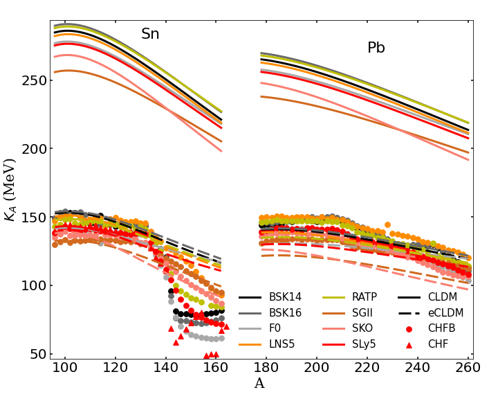
In Fig. 3, we show as function of $A$, for Sn and Pb isotopes, the comparison of the CLDM (solid lines) and eCLDM (53) (dashed lines) predictions against the microscopic predictions (circles) for $K_{A}$, based on the constrained Hartree-Fock-Bogoliubov (CHFB) approach, for the set of Skyrme interaction listed in Tab. 2 (see Refs. Khan et al. 2012; Khan and Margueron 2013 for more details on the microscopic CHFB approach). We use the microscopic radii calculated by each interaction, to transform $E_{\mathrm{ISGMR}}$ into $K_{A}$ using Eq. (1). For SLy5, our results are identical to the ones given in Ref. Khan et al. 2013. By comparing CHF (red triangles) and CHFB (red circles), we see that pairing contributes to reduce the shell effects around $A\approx 140$ in Sn and makes the isotopic evolution of $K_{A}$ smoother.

As stated by Blaizot Blaizot 1980, the CLDM predictions are largely overestimating $K_{A}$, since the surface energy is not explicitly density-dependent. By adding the new term (50) for the surface energy (Eq. (62)), the eCLDM reproduces the isotopic dependence of $K_{A}$ as predicted by the microscopic CHFB approach (note that only one nucleus (¹⁰⁰Sn) has been used for the calibration of $a_{\mathrm{surf}}$).

In Sn isotopes, one can note a marked step for $K_{A}$ for $A\gtrsim 132$, in microscopic predictions, which is not present in the eCLDM prediction. The eCLDM predicts instead a continuous decrease of $K_{A}$ over the isotopic chain. A similar feature, while not as pronounced, is observed for Pb isotopes for $A\gtrsim 208$. Microscopically, these steps are understood as originating from shell effects: in ¹³²Sn, they are 12 occupied 1h_11/2 states below the Fermi level and 10 unoccupied 1h_9/2 states. For ²⁰⁸Pb, the Fermi level is for $1i_{13/2}$ and the next orbital is $1i_{11/2}$. The $\Delta L=0$ isoscalar oscillation is therefore enhanced for neutron-rich systems belonging to these two isotopic chains. Since shell effects are not present in the eCLDM, such steps could not be described by our macroscopic approach. The decrease of $K_{A}$ as nuclei get more and more neutron-rich is however well reproduced by the eCLDM approach. Such a dependence on $A$ depends on the choice of the NEP, as illustrated in the appendix section A.5.

As a first application of the eCLDM, we compute the binding energies, the incompressibilities $K_{A}$ and ISGMR energies for several Sn and Pb isotopes and for the SLy5 Skyrme interaction (see Tab. 3). All these quantities are given for both the eCLDM and the CLDM approaches. Experimental data for the binding energies from AME2020 table Huang et al. 2021 are also given. We have also calculated the ratio $c_{A}=K_{A,\mathrm{surf}}/K_{\mathrm{sat}}$ for the set of nuclei. Interestingly, we found $c_{A}\approx-1.3$, which is compatible with the calculations of Ref. Patra et al. 2002 deduced from a microscopic approach. Consistently with Fig. 3, the value obtained for $K_{A}$ with the eCLDM is considerably reduced, compared to the one provided from the CLDM, illustrating the impact of the density-dependent surface energy term. $K_{\mathrm{surf}}$ is also given in Tab. 3. The contribution of the density-dependent surface energy term is large: it changes the sign of the term $K_{\mathrm{surf}}$, from positive (CLDM) to negative (eCLDM). The $A$ dependence of $K_{\mathrm{surf}}$ is also strongly modified with the density-dependent surface energy term. The value for $K_{\mathrm{Coul}}$ is not much impacted by the density-dependent surface energy term. In addition, $K_{\mathrm{Coul}}$ is compatible with the value extracted from the liquid drop expansion Sagawa et al. 2007 and are rather insensitive to the nuclear interaction. Finally, we show, in the last column, the values for ISGMR energies. Since this values are directly impacted by $K_{A}$, see Eq. (1), the eCLDM shows a reduction for the $E_{\rm ISGMR}$ energies. Note that this reduction makes the eCLDM results closer to the experimental values.

Tab. 3 illustrates one of the main feature of the eCLDM approach: the present density-dependent surface energy term has a small impact on the binding energies, but a large contribution to the incompressibility modulus $K_{A}$ in finite nuclei. This justifies our fitting protocol previously described. It also shows that the low order NEP could be adjusted to the nuclear mass table quite independently to the higher order NEP which are fitted to $K_{A}$.

We aim at reproducing together the values of $K_{A}$ in ^90,92Zr, ^112-124Sn, ^204-208Pb from Ref. Garg and Coló 2018, see Tab. 4 for detailed values. We do not consider here the experimental GMR energy measured for ⁹⁴Zr and reported in Ref. Garg and Coló 2018, since it is very different from the one measured in ⁹⁰Zr and ⁹²Zr. It is not possible, for our modeling to reproduce this data, as it is shown hereafter in Fig. 7. In addition, we investigate the role of a fictitious measurement of the GMR energy in ¹³²Sn and explore possible consequences for the determination of NEP.

We first report, in Tab. 4, the experimental data listed in Ref. Garg and Coló 2018. For some nuclei there are different values obtained from different experiments, see for instance ⁹⁰Zr, ⁹²Zr, ¹¹²Sn and ¹²⁴Sn (the largest differences between different experimental measurements are for ¹¹²Sn and ¹²⁴Sn). In the following, we adopt an agnostic approach w.r.t. these data and we then equally treat the measurements. It should be noted that we have then re-calculated averaged centroids and standard deviations for nuclei were two experimental values are reported, generating a new distribution summing the individual ones. We have then determined the value for $K_{A}$ using Eq. (1), where the total radius $R_{A}$ is provided by an CHFB calculation Bennaceur and Dobaczewski 2005 using SLy5 Chabanat et al. 1998 Skyrme interaction. The last column in Tab. 4 gives the experimental values for $K_{A}$ which are used in the confrontation of our eCLDM to nuclear data.

In this subsection, we vary a set of NEP in order to determine the best parameters reproducing the experimental data. We first present the experimental data and then the Markov-chain Monte Carlo (MCMC) approach we adopt.

The confrontation between the experimental data for the incompressibility $K_{A}$ (see tab. 4), and the model predictions, is based on the loss functions $\chi_{K_{A}}$, which is defined as

References

- van der Woude and Harakeh (2001) A. van der Woude and M. Harakeh, Giant Resonances: Fundamental High-frequency Modes of Nuclear Excitation (Oxford University Press, 2001).
- Rezzolla et al. (2018) L. Rezzolla, P. A. M. Pizzochero, D. I. Jones, N. Rea, and I. Vidaña, The Physics and Astrophysics of Neutron Stars, Vol. 457 (Springer International Publishing, 2018).
- Margueron et al. (2018a) J. Margueron, R. Hoffmann Casali, and F. Gulminelli, Phys. Rev. C 97, 025805 (2018a).
- Blaizot (1980) J. P. Blaizot, Phys. Rep. 64, 171 (1980).
- Garg and Coló (2018) U. Garg and G. Coló, Progress in Particle and Nuclear Physics 101, 55 (2018).
- Huang et al. (2021) W. Huang, M. Wang, F. Kondev, G. Audi, and S. Naimi, Chinese Physics C 45, 030002 (2021).
- Li and Xie (2021) B.-A. Li and W.-J. Xie, Phys. Rev. C 104, 034610 (2021).
- Patra et al. (2002) S. K. Patra, M. Centelles, X. Viñas, and M. Del Estal, Phys. Rev. C 65, 044304 (2002).
- Sagawa et al. (2007) H. Sagawa, S. Yoshida, G. Zeng, J. Gu, and X. Zhang, Phys. Rev. C 76, 034327 (2007).
- Avogadro and Bertulani (2013) P. Avogadro and C. A. Bertulani, Phys. Rev. C 88, 044319 (2013).
- Goriely et al. (2009) S. Goriely, S. Hilaire, M. Girod, and S. Péru, Phys. Rev. Lett. 102, 242501 (2009).
- Lalazissis et al. (2005) G. A. Lalazissis, T. Nikšić, D. Vretenar, and P. Ring, Phys. Rev. C 71, 024312 (2005).
- Khan et al. (2012) E. Khan, J. Margueron, and I. Vidaña, Phys. Rev. Lett. 109, 092501 (2012).
- Khan and Margueron (2013) E. Khan and J. Margueron, Phys. Rev. C 88, 034319 (2013).
- Margueron and Gulminelli (2019) J. Margueron and F. Gulminelli, Phys. Rev. C 99, 025806 (2019).
- Myers and Swiatecki (1969) W. D. Myers and W. J. Swiatecki, Ann. Phys. 55, 395 (1969).
- Weiss and Cameron (1969) R. A. Weiss and A. G. W. Cameron, Can. J. Phys. 47, 2171 (1969).
- Baym et al. (1971) G. Baym, H. A. Bethe, and C. Pethick, Nucl. Phys. A 175, 225 (1971).
- Steiner (2008) A. W. Steiner, Phys. Rev. C 77, 035805 (2008).
- Carreau et al. (2019) T. Carreau, F. Gulminelli, and J. Margueron, Eur. Phys. J. A 55, 188 (2019).
- Grams et al. (2022a) G. Grams, R. Somasundaram, J. Margueron, and S. Reddy, Phys. Rev. C 105, 035806 (2022a).
- Grams et al. (2022b) G. Grams, J. Margueron, R. Somasundaram, and S. Reddy, Eur. Phys. J. A 58, 56 (2022b).
- Somasundaram et al. (2021a) R. Somasundaram, C. Drischler, I. Tews, and J. Margueron, Phys. Rev. C 103, 045803 (2021a).
- Goriely et al. (2007) S. Goriely, M. Samyn, and J. M. Pearson, Phys. Rev. C 75, 064312 (2007).
- Chamel et al. (2008) N. Chamel, S. Goriely, and J. Pearson, Nucl Phys. A 812, 72 (2008).
- Lesinski et al. (2006) T. Lesinski, K. Bennaceur, T. Duguet, and J. Meyer, Phys. Rev. C 74, 044315 (2006).
- Cao et al. (2006) L. G. Cao, U. Lombardo, C. W. Shen, and N. V. Giai, Phys. Rev. C 73, 014313 (2006).
- Rayet et al. (1982) M. Rayet, M. Arnould, F. Tondeur, and G. Paulus, Astron. Astrophys. 116, 183 (1982).
- Van Giai and Sagawa (1981) N. Van Giai and H. Sagawa, Physics Letters B 106, 379 (1981).
- Reinhard and Flocard (1995) P.-G. Reinhard and H. Flocard, Nuclear Physics A 584, 467 (1995).
- Reinhard et al. (1999) P.-G. Reinhard, D. J. Dean, W. Nazarewicz, J. Dobaczewski, J. A. Maruhn, and M. R. Strayer, Phys. Rev. C 60, 014316 (1999).
- Chabanat et al. (1998) E. Chabanat, P. Bonche, P. Haensel, J. Meyer, and R. Schaeffer, Nucl. Phys. A 635, 231 (1998).
- Piekarewicz and Centelles (2009) J. Piekarewicz and M. Centelles, Phys. Rev. C 79, 054311 (2009).
- Papakonstantinou et al. (2013) P. Papakonstantinou, J. Margueron, F. Gulminelli, and A. R. Raduta, Phys. Rev. C 88, 045805 (2013).
- d’Etivaux et al. (2019) N. B. d’Etivaux, S. Guillot, J. Margueron, N. Webb, M. Catelan, and A. Reisenegger, The Astrophysical Journal 887, 48 (2019).
- Sagawa et al. (2019) H. Sagawa, S. Yoshida, and L.-G. Cao, AIP Conference Proceedings 2127, 020002 (2019), https://aip.scitation.org/doi/pdf/10.1063/1.5117792 .
- Tews et al. (2017) I. Tews, J. M. Lattimer, A. Ohnishi, and E. E. Kolomeitsev, The Astrophysical Journal 848, 105 (2017).
- Li et al. (2010) T. Li, U. Garg, Y. Liu, R. Marks, B. K. Nayak, P. V. Madhusudhana Rao, M. Fujiwara, H. Hashimoto, K. Nakanishi, S. Okumura, M. Yosoi, M. Ichikawa, M. Itoh, R. Matsuo, T. Terazono, M. Uchida, Y. Iwao, T. Kawabata, T. Murakami, H. Sakaguchi, S. Terashima, Y. Yasuda, J. Zenihiro, H. Akimune, K. Kawase, and M. N. Harakeh, Phys. Rev. C 81, 034309 (2010).
- Khan et al. (2013) E. Khan, N. Paar, D. Vretenar, L.-G. Cao, H. Sagawa, and G. Colò, Phys. Rev. C 87, 064311 (2013).
- Carson et al. (2019) Z. Carson, A. W. Steiner, and K. Yagi, Phys. Rev. D 99, 043010 (2019).
- Möller et al. (2012) P. Möller, W. D. Myers, H. Sagawa, and S. Yoshida, Phys. Rev. Lett. 108, 052501 (2012).
- Li et al. (2021) B.-A. Li, B.-J. Cai, W.-J. Xie, and N.-B. Zhang, Universe 7 (2021), 10.3390/universe7060182.
- Iida and Oyamatsu (2004) K. Iida and K. Oyamatsu, Phys. Rev. C 69, 037301 (2004).
- Bennaceur and Dobaczewski (2005) K. Bennaceur and J. Dobaczewski, Computer Physics Communications 168, 96 (2005).
- Ota et al. (2017) S. Ota et al., Riken Accel. Prog. Rep. 50, 1 (2017).
- Margueron et al. (2018b) J. Margueron, R. Hoffmann Casali, and F. Gulminelli, Phys. Rev. C 97, 025805 (2018b), arXiv:1708.06894 [nucl-th] .
- Reed et al. (2021) B. T. Reed, F. J. Fattoyev, C. J. Horowitz, and J. Piekarewicz, Phys. Rev. Lett. 126, 172503 (2021).
- Drischler et al. (2020) C. Drischler, R. J. Furnstahl, J. A. Melendez, and D. R. Phillips, Phys. Rev. Lett. 125, 202702 (2020), arXiv:2004.07232 [nucl-th] .
- Danielewicz et al. (2002) P. Danielewicz, R. Lacey, and W. G. Lynch, Science 298, 1592 (2002), arXiv:nucl-th/0208016 .
- Hinderer (2008) T. Hinderer, Astrophys. J. 677, 1216 (2008), arXiv:0711.2420 [astro-ph] .
- Flanagan and Hinderer (2008) E. E. Flanagan and T. Hinderer, Phys. Rev. D 77, 021502 (2008), arXiv:0709.1915 [astro-ph] .
- Somasundaram et al. (2021b) R. Somasundaram, I. Tews, and J. Margueron, (2021b), arXiv:2112.08157 [nucl-th] .
- Han and Steiner (2019) S. Han and A. W. Steiner, Phys. Rev. D 99, 083014 (2019), arXiv:1810.10967 [nucl-th] .
- Bohr and Mottelson (1969) A. Bohr and B. R. Mottelson, Nuclear structure vol I (Addison-Wesley, 1969).
- Vogel et al. (1984) P. Vogel, B. Jonson, and P. Hansen, Physics Letters B 139, 227 (1984).
- Lattimer and Swesty (1991) J. M. Lattimer and D. Swesty, Nuclear Phys. A 535, 331 (1991).
- Colo‘ and Van Giai (2004) G. Colo‘ and N. Van Giai, Nuclear Physics A 731, 15 (2004).
- Garg et al. (2007) U. Garg, T. Li, S. Okumura, H. Akimune, M. Fujiwara, M. Harakeh, H. Hashimoto, M. Itoh, Y. Iwao, T. Kawabata, K. Kawase, Y. Liu, R. Marks, T. Murakami, K. Nakanishi, B. Nayak, P. Madhusudhana Rao, H. Sakaguchi, Y. Terashima, M. Uchida, Y. Yasuda, M. Yosoi, and J. Zenihiro, Nuclear Physics A 788, 36 (2007).
- Patel et al. (2012) D. Patel, U. Garg, M. Fujiwara, H. Akimune, G. Berg, M. Harakeh, M. Itoh, T. Kawabata, K. Kawase, B. Nayak, T. Ohta, H. Ouchi, J. Piekarewicz, M. Uchida, H. Yoshida, and M. Yosoi, Physics Letters B 718, 447 (2012).