跳到论文正文
W Papers独立论文阅读器 arXiv:2207.01796 论文正文 计算阅读时间 · 0%
引用这篇论文根据当前论文元数据生成,正式投稿前建议核对。


License: arXiv.org perpetual non-exclusive license
arXiv:2207.01796v2 [cs.RO] 16 May 2023
\AtNextBibliography

[Uncaptioned image]
Manipulator
Differential Kinematics
Part I: Kinematics and Velocity

By Jesse Haviland and Peter Corke

Manipulator kinematics is concerned with the motion of each link within a manipulator without considering mass or force. This article, which is the first in a two-part tutorial, provides an introduction into modelling manipulators using the elementary transform sequence (ETS) and then formulates the first order differential kinematics. The first order differential kinematics leads to the manipulator Jacobian which is the basis for velocity control and inverse kinematics. We describe important classical techniques which rely on the manipulator Jacobian before exhibiting some contemporary applications. Part 2 of this tutorial provides a formulation of second and higher order differential kinematics, introduces the manipulator Hessian, and illustrates advanced techniques, some of which improve the performance of techniques demonstrated in Part 1.

A serial-link manipulator, which we refer to as a manipulator in this article, is the formal name for a robot which comprises a chain of rigid links and joints which may contain parallel branches, but not form a closed loop. Each joint provides one degree of freedom, which may be a prismatic joint providing translational freedom or a revolute joint providing rotational freedom. The base frame of a manipulator represents the reference frame of the first link in the chain while the last link is known as the end-effector.

Manipulator kinematics is an essential area of study and provides the foundation for robotic control. The motion of each joint within a manipulator modifies the pose of each subsequent joint, and ultimately the pose of the end-effector. This relationship forms the basis of all kinematic equations. This article formulates kinematic equations using ETS notation.

Refer to caption
Figure 1: The Elementary Transform Sequence of the 7 degree-of-freedom Franka-Emika Panda serial-link manipulator in its zero-angle configurations. 𝐄i{{\mathbf{E}}}_{i} represents an elementary transform while ξba{}^{a}{\mathbf{\xi}}_{b} represents the pose of link frame bb in the reference frame of link aa.
Refer to caption
Figure 2: The six elementary transforms 𝐄∈𝐒𝐄⁡(3){{\mathbf{E}}}\in\mathrm{{\bf SE}(3)} from (2) which are the building blocks for ETS notation. Each homogeneous transformation matrix above represents a translation along, or a rotation about, a single axis which is parameterized by η\eta as defined in (3) and (4)

The ETS, introduced in [2], provides a universal method for describing the kinematics of any manipulator. This intuitive and systematic approach can be applied with a simple walk through procedure. The resulting sequence comprises a number of elementary transforms – translations and rotations – from the base frame to the robot’s end-effector. An example of an ETS is displayed in Figure 1 for the Franka-Emika Panda in its zero-angle configuration.

The ETS is conceptually easy to grasp, since it avoids the frame assignment constraints of Denavit and Hartenberg (DH) notation [4], and allows joint rotation or translation about or along any axis.

We have provided Jupyter Notebooks to accompany each section within this tutorial. The Notebooks are written in Python code and use the Robotics Toolbox for Python and the Swift Simulator [1] to provide examples and implementations of algorithms. While not absolutely essential, for the most engaging and informative experience, we recommend working through the Jupyter Notebooks concurrently while reading this article.

We use the notation of [3] where {a}\{\mathrm{a}\} denotes a coordinate frame, and 𝐓ba{}^{a}{{\mathbf{T}}}_{b} is a relative pose or rigid-body transformation of {b}\{\mathrm{b}\} with respect to {a}\{\mathrm{a}\}.

Refer to caption
Figure 3: Shown on the left is a vector 𝒔∈ℝ3{\bm{s}}\in\mathbb{R}^{3} along with its corresponding skew symmetric matrix 𝐒∈\so​3⊂ℝ3×3{{\mathbf{S}}}\in\so{3}\subset\mathbb{R}^{3\times 3}. Shown on the right is a vector 𝒔^∈ℝ6{\hat{{\bm{s}}}}\in\mathbb{R}^{6} along with its corresponding augmented skew symmetric matrix 𝐒^∈𝐬𝐞⁡(3)⊂ℝ4×4{\hat{\mathbf{S}}}\in\mathrm{{\bf se}(3)}\subset\mathbb{R}^{4\times 4}. The skew functions [⋅]×:ℝ3↦\so​3\left[\cdot\right]_{\times}:\mathbb{R}^{3}\mapsto\so{3} maps a vector to a skew symmetric matrix, and [⋅]:ℝ6↦𝐬𝐞⁡(3)\left[\cdot\right]:\mathbb{R}^{6}\mapsto\mathrm{{\bf se}(3)} maps a vector to an augmented skew symmetric matrix. The inverse skew functions ∨×(⋅):\so3↦ℝ3\vee_{\times}\left(\cdot\right):\so{3}\mapsto\mathbb{R}^{3} maps a skew symmetric matrix to a vector and ∨(⋅):𝐬𝐞⁡(3)↦ℝ6\vee\left(\cdot\right):\mathrm{{\bf se}(3)}\mapsto\mathbb{R}^{6} maps an augmented skew symmetric matrix to a vector.

Forward Kinematics

The forward kinematics is the first and most basic relationship between the link geometry and robot configuration.

The forward kinematics of a manipulator provides a non-linear mapping

𝐓⁡(t)=𝒦⁡(𝒒⁡(t)){{\mathbf{T}}}(t)={\cal K}({\bm{q}}(t))

between the joint space and Cartesian task space, where 𝒒(t)=(q1(t),q2(t),⋯qn(t))∈ℝn{\bm{q}}(t)=(q_{1}(t),q_{2}(t),\cdots q_{n}(t))\in\mathbb{R}^{n} is the vector of joint generalised coordinates, nn is the number of joints, and 𝐓∈𝐒𝐄⁡(3){{\mathbf{T}}}\in\mathrm{{\bf SE}(3)} is a homogeneous transformation matrix representing the pose of the robot’s end-effector in the world-coordinate frame. The ETS model defines 𝒦⁡(⋅)\cal{K}(\cdot) as the product of MM elementary transforms 𝐄i∈𝐒𝐄⁡(3){{\mathbf{E}}}_{i}\in\mathrm{{\bf SE}(3)}

𝐓⁡(t)\displaystyle{{\mathbf{T}}}(t) =𝐄1​(η1)​𝐄2​(η2)​…​𝐄M​(ηM)\displaystyle={{\mathbf{E}}}_{1}(\eta_{1}){{\mathbf{E}}}_{2}(\eta_{2})\ldots{{\mathbf{E}}}_{M}(\eta_{M})
=∏i=1M𝐄i​(ηi).\displaystyle=\prod_{i=1}^{M}{{\mathbf{E}}}_{i}(\eta_{i}). (1)

Each of the elementary transforms 𝐄i{{\mathbf{E}}}_{i} can be a pure translation along, or a pure rotation about the local x-, y-, or z-axis by an amount ηi\eta_{i}. Explicitly, each transform is one of the following

𝐄i={𝐓𝒕x​(ηi)𝐓𝒕y​(ηi)𝐓𝒕z​(ηi)𝐓𝐑x​(ηi)𝐓𝐑y​(ηi)𝐓𝐑z​(ηi){{\mathbf{E}}}_{i}=\left\{\begin{matrix}{{\mathbf{T}}}_{{\!{\bm{t}}}_{x}}(\eta_{i})\\ {{\mathbf{T}}}_{{\!{\bm{t}}}_{y}}(\eta_{i})\\ {{\mathbf{T}}}_{{\!{\bm{t}}}_{z}}(\eta_{i})\\ {{\mathbf{T}}}_{{\!{{\mathbf{R}}}}_{x}}(\eta_{i})\\ {{\mathbf{T}}}_{{\!{{\mathbf{R}}}}_{y}}(\eta_{i})\\ {{\mathbf{T}}}_{{\!{{\mathbf{R}}}}_{z}}(\eta_{i})\\ \end{matrix}\right. (2)

where each of the matrices are displayed in Figure 2 and the parameter ηi\eta_{i} is either a constant cic_{i} (translational offset or rotation) or a joint variable qj​(t)q_{j}(t)

ηi={ciqj​(t)\eta_{i}=\left\{\begin{matrix}c_{i}\\ q_{j}(t)\\ \end{matrix}\right. (3)

and the joint variable is

qj(t)={θ⁡(t)for a revolute jointd⁡(t)for a prismatic jointq_{j}(t)=\left\{\begin{matrix}[l]\theta(t)&\quad\mbox{for a revolute joint}\\ d(t)&\quad\mbox{for a prismatic joint}\\ \end{matrix}\right. (4)

where θ⁡(t)\theta(t) represents a joint angle, and d⁡(t)d(t) represents a joint translation.

An ETS description does not require intermediate link frames, but it does not preclude their introduction. The convention we adopt is to place the jt​hj^{th} frame immediately after the ETS term related to qjq_{j}, as shown in Figure 1. The relative transform between link frames aa and bb is simply a subset of the ETS

𝐓ba{}^{a}{{\mathbf{T}}}_{b} =∏i=μ⁡(a)μ⁡(b)𝐄i​(ηi)\displaystyle=\prod_{i=\mu(a)}^{\mu(b)}{{\mathbf{E}}}_{i}(\eta_{i}) (5)

where the function μ⁡(j)\mu(j) returns the index in the ETS expression, (Forward Kinematics) in this case, which corresponds to the link frame jj. For example, from Figure 1, for joint variable j=5j=5, μ⁡(j)=10\mu(j)=10.

Deriving the Manipulator Jacobian

First Derivative of a Pose

Now consider the end-effector pose, which varies as a function of joint coordinates. The derivative with respect to time is

𝐓˙=d​𝐓d​t=∂𝐓∂q1​q˙1+⋯+∂𝐓∂qn​q˙n∈ℝ4×4\dot{{{\mathbf{T}}}}=\frac{\mathrm{d}{{\mathbf{T}}}}{\mathrm{d}t}=\frac{\partial{{\mathbf{T}}}}{\partial q_{1}}\dot{q}_{1}+\cdots+\frac{\partial{{\mathbf{T}}}}{\partial q_{n}}\dot{q}_{n}\in\mathbb{R}^{4\times 4} (6)

where each ∂𝐓∂qi∈ℝ4×4\frac{\partial{{\mathbf{T}}}}{\partial q_{i}}\in\mathbb{R}^{4\times 4}.

The information in 𝐓{{\mathbf{T}}} is non-minimal, and redundant, as is the information in 𝐓˙\dot{{{\mathbf{T}}}}. We can write these respectively as

𝐓=(𝐑𝒕01),𝐓˙=(𝐑˙𝒕˙00){{\mathbf{T}}}=\begin{pmatrix}{{\mathbf{R}}}&{\bm{t}}\\ 0&1\end{pmatrix},\,\,\,\dot{{{\mathbf{T}}}}=\begin{pmatrix}\dot{{{\mathbf{R}}}}&\dot{{\bm{t}}}\\ 0&0\end{pmatrix} (7)

where 𝐑∈𝐒𝐎⁡(3){{\mathbf{R}}}\in\mathrm{{\bf SO}(3)}, 𝐑˙∈ℝ3×3\dot{{{\mathbf{R}}}}\in\mathbb{R}^{3\times 3}, and 𝒕,𝒕˙∈ℝ3{\bm{t}},\dot{{\bm{t}}}\in\mathbb{R}^{3}.

We will write the partial derivative in partitioned form as

∂𝐓∂qj=(𝐉Rj𝐉tj00)\frac{\partial{{\mathbf{T}}}}{\partial q_{j}}=\begin{pmatrix}{{\mathbf{J}_{\!R}}}_{j}&{{\mathbf{J}_{\!t}}}_{j}\\ 0&0\end{pmatrix} (8)

where 𝐉Rj∈ℝ3×3{{\mathbf{J}_{\!R}}}_{j}\in\mathbb{R}^{3\times 3} and 𝐉tj∈ℝ3×1{{\mathbf{J}_{\!t}}}_{j}\in\mathbb{R}^{3\times 1}, and then rewrite (6) as

(𝐑˙𝒕˙00)=(𝐉R1𝐉t100)​q˙1+⋯+(𝐉Rn𝐉tn00)​q˙n\begin{pmatrix}\dot{{{\mathbf{R}}}}&\dot{{\bm{t}}}\\ 0&0\end{pmatrix}=\begin{pmatrix}{{\mathbf{J}_{\!R}}}_{1}&{{\mathbf{J}_{\!t}}}_{1}\\ 0&0\end{pmatrix}\dot{q}_{1}+\cdots+\begin{pmatrix}{{\mathbf{J}_{\!R}}}_{n}&{{\mathbf{J}_{\!t}}}_{n}\\ 0&0\end{pmatrix}\dot{q}_{n}\,\,

and write a matrix equation for each non-zero partition

𝐑˙\displaystyle\dot{{{\mathbf{R}}}} =𝐉R1​q˙1+⋯+𝐉Rn​q˙n\displaystyle={{\mathbf{J}_{\!R}}}_{1}\dot{q}_{1}+\cdots+{{\mathbf{J}_{\!R}}}_{n}\dot{q}_{n} (9)
𝒕˙\displaystyle\dot{{\bm{t}}} =𝐉t1​q˙1+⋯+𝐉tn​q˙n\displaystyle={{\mathbf{J}_{\!t}}}_{1}\dot{q}_{1}+\cdots+{{\mathbf{J}_{\!t}}}_{n}\dot{q}_{n} (10)

where each term represents the contribution to end-effector velocity due to motion of the corresponding joint.

Taking (10) first, we can simply write

𝒕˙\displaystyle\dot{{\bm{t}}} =(𝐉t1⋯𝐉tn)​(q˙1q˙n)\displaystyle=\begin{pmatrix}{{\mathbf{J}_{\!t}}}_{1}&\cdots&{{\mathbf{J}_{\!t}}}_{n}\end{pmatrix}\begin{pmatrix}\dot{q}_{1}\\ \vdots\\ \dot{q}_{n}\end{pmatrix}
=𝐉v​(𝒒)​𝒒˙\displaystyle={{\mathbf{J}}}_{v}({\bm{q}})\dot{{\bm{q}}} (11)

where 𝐉v​(𝒒)∈ℝ3×n{{\mathbf{J}}}_{v}({\bm{q}})\in\mathbb{R}^{3\times n} is the translational part of the manipulator Jacobian.

Rotation rate is slightly more complex, but using the identity 𝐑˙=[𝝎]×​𝐑\dot{{{\mathbf{R}}}}=\left[\bm{\omega}\right]_{\times}{{\mathbf{R}}} where 𝝎∈ℝ3{\bm{\omega}}\in\mathbb{R}^{3} is the angular velocity, and [𝝎]×∈\so​3\left[\bm{\omega}\right]_{\times}\in\so{3} is a skew-symmetric matrix, we can rewrite (9) as

[𝝎]×​𝐑=𝐉R1​q˙1+⋯+𝐉Rn​q˙n\left[\bm{\omega}\right]_{\times}{{\mathbf{R}}}={{\mathbf{J}_{\!R}}}_{1}\dot{q}_{1}+\cdots+{{\mathbf{J}_{\!R}}}_{n}\dot{q}_{n} (12)

and rearrange to

[𝝎]×=(𝐉R1​𝐑⊤)​q˙1+⋯+(𝐉Rn​𝐑⊤)​q˙n∈\so​3\left[\bm{\omega}\right]_{\times}=({{\mathbf{J}_{\!R}}}_{1}{{\mathbf{R}}}^{\top})\dot{q}_{1}+\cdots+({{\mathbf{J}_{\!R}}}_{n}{{\mathbf{R}}}^{\top})\dot{q}_{n}\in\so{3}

where each of the terms 𝐉Rj​𝐑⊤{{\mathbf{J}_{\!R}}}_{j}{{\mathbf{R}}}^{\top} must also be skew-symmetric since the sum of skew-symmetric matrices is skew-symmetric. This 3×33\times 3 matrix equation therefore has only 3 unique equations so applying the inverse skew operator to both sides we have

𝝎\displaystyle{\bm{\omega}} =∨×(𝐉R1𝐑⊤)q˙1+⋯+∨×(𝐉Rn𝐑⊤)q˙n\displaystyle=\vee_{\times}\left({{\mathbf{J}_{\!R}}}_{1}{{\mathbf{R}}}^{\top}\right)\dot{q}_{1}+\cdots+\vee_{\times}\left({{\mathbf{J}_{\!R}}}_{n}{{\mathbf{R}}}^{\top}\right)\dot{q}_{n}
=(∨×(𝐉R1𝐑⊤)⋯∨×(𝐉Rn𝐑⊤))​(q˙1q˙n)\displaystyle=\bigg(\begin{matrix}\vee_{\times}\left({{\mathbf{J}_{\!R}}}_{1}{{\mathbf{R}}}^{\top}\right)&\cdots&\vee_{\times}\left({{\mathbf{J}_{\!R}}}_{n}{{\mathbf{R}}}^{\top}\right)\end{matrix}\bigg)\begin{pmatrix}\dot{q}_{1}\\ \vdots\\ \dot{q}_{n}\end{pmatrix}
=𝐉ω​(𝒒)​𝒒˙\displaystyle={{\mathbf{J}_{\!\omega}}}({\bm{q}})\dot{{\bm{q}}} (13)

where 𝐉ω​(𝒒)∈ℝ3×n{{\mathbf{J}_{\!\omega}}}({\bm{q}})\in\mathbb{R}^{3\times n} is the rotational part of the manipulator Jacobian.

Combining (11) and (First Derivative of a Pose) we can write

𝝂=(𝒗𝝎)=(𝐉v​(𝒒)𝐉ω​(𝒒))​𝒒˙{\bm{\nu}}=\begin{pmatrix}{\bm{v}}\\ \bm{\omega}\end{pmatrix}=\begin{pmatrix}{{\mathbf{J}}}_{v}({\bm{q}})\\ {{\mathbf{J}_{\!\omega}}}({\bm{q}})\end{pmatrix}\dot{{\bm{q}}} (14)

which expresses end-effector velocity in terms of joint velocity

𝐉0​(𝒒)=(𝐉v​(𝒒)𝐉ω​(𝒒))∈ℝ6×n{{}^{0}{{\mathbf{J}}}}({\bm{q}})=\begin{pmatrix}{{\mathbf{J}}}_{v}({\bm{q}})\\ {{\mathbf{J}_{\!\omega}}}({\bm{q}})\end{pmatrix}\in\mathbb{R}^{6\times n} (15)

is the manipulator Jacobian matrix expressed in the world-coordinate frame. We can calculate the Jacobian expressed in the end-effector frame as

𝐉e​(𝒒)=(𝐑e⊤0𝟎𝟎𝐑e⊤0)​𝐉0​(𝒒){{}^{e}{{\mathbf{J}}}}({\bm{q}})=\begin{pmatrix}{{{}^{0}{{\mathbf{R}}}}_{e}^{\top}}&\mathbf{0}\\ \mathbf{0}&{{{}^{0}{{\mathbf{R}}}}_{e}^{\top}}\end{pmatrix}{{}^{0}{{\mathbf{J}}}}({\bm{q}}) (16)

where 𝐑e0=ρ(0𝐓e){{}^{0}{{\mathbf{R}}}}_{e}=\rho(^{0}{{\mathbf{T}}}_{e}) is the matrix which represents the rotation of the end-effector in the world frame.

More compactly we write

𝝂=𝐉0​(𝒒)​𝒒˙{\bm{\nu}}={{}^{0}{{\mathbf{J}}}}({\bm{q}})\dot{{\bm{q}}} (17)

which provides the derivative of the left side of (Forward Kinematics).

However, in order to compute (17), we need to first find the partial derivative of a pose with respect to a joint coordinate.

First Derivative of an Elementary
Transform

Before differentiating the ETS to find the manipulator Jacobian, it is useful to consider the derivative of a single Elementary Transform. In this section we use the skew and inverse skew operation as defined in Figure 3.

Derivative of a Rotation

The derivative of a rotation matrix with respect to the rotation angle θ\theta is required when considering a revolute joint and can be shown to be

d​𝐑​(θ)d​θ\displaystyle\frac{\mathrm{d}{{\mathbf{R}}}(\theta)}{\mathrm{d}\theta} =[𝝎^]×​𝐑​(θ⁡(t))\displaystyle=\left[{\hat{{\bm{\omega}}}}\right]_{\times}{{\mathbf{R}}}(\theta(t)) (18)

where the unit vector 𝝎^{\hat{{\bm{\omega}}}} is the joint rotation axis.

The rotation axis 𝝎^{\hat{{\bm{\omega}}}} can be recovered using the inverse skew operator

𝝎^\displaystyle{\hat{{\bm{\omega}}}} =∨×(d​𝐑​(θ)d​θ𝐑(θ(t))⊤)\displaystyle=\vee_{\times}\left(\frac{\mathrm{d}{{{{\mathbf{R}}}}\left(\theta\right)}}{\mathrm{d}\theta}{{{{\mathbf{R}}}}\left(\theta(t)\right)}^{\top}\right) (19)

since 𝐑∈𝐒𝐎⁡(3){{\mathbf{R}}}\in\mathrm{{\bf SO}(3)}, then 𝐑−1=𝐑⊤{{\mathbf{R}}}^{-1}={{\mathbf{R}}}^{\top}.

For an ETS, we only need to consider the elementary rotations 𝐑x{{\mathbf{R}}}_{x}, 𝐑y{{\mathbf{R}}}_{y}, and 𝐑z{{\mathbf{R}}}_{z} which are embedded within 𝐒𝐄⁡(3)\mathrm{{\bf SE}(3)}, as 𝐓𝐑x{{\mathbf{T}}}_{{\!{{\mathbf{R}}}}_{x}}, 𝐓𝐑y{{\mathbf{T}}}_{{\!{{\mathbf{R}}}}_{y}}, and 𝐓𝐑z{{\mathbf{T}}}_{{\!{{\mathbf{R}}}}_{z}} i.e. pure rotations with no translational component. We can show that the derivative of each elementary rotation with respect to a rotation angle is

d​𝐓𝐑x​(θ)d​θ\displaystyle\dfrac{\mathrm{d}{{\mathbf{T}}}_{{\!{{\mathbf{R}}}}_{x}}(\theta)}{\mathrm{d}\theta} =(000000−1001000000)​𝐓𝐑x​(θ)=[𝑹^x]​𝐓𝐑x​(θ),\displaystyle=\begin{pmatrix}0&0&0&0\\ 0&0&-1&0\\ 0&1&0&0\\ 0&0&0&0\end{pmatrix}{{\mathbf{T}}}_{{\!{{\mathbf{R}}}}_{x}}(\theta)=\big[{\hat{{\bm{R}}}}_{x}\big]{{\mathbf{T}}}_{{\!{{\mathbf{R}}}}_{x}}(\theta), (20)
d​𝐓𝐑y​(θ)d​θ\displaystyle\dfrac{\mathrm{d}{{\mathbf{T}}}_{{\!{{\mathbf{R}}}}_{y}}(\theta)}{\mathrm{d}\theta} =(00100000−10000000)​𝐓𝐑y​(θ)=[𝑹^y]​𝐓𝐑y​(θ),\displaystyle=\begin{pmatrix}0&0&1&0\\ 0&0&0&0\\ -1&0&0&0\\ 0&0&0&0\end{pmatrix}{{\mathbf{T}}}_{{\!{{\mathbf{R}}}}_{y}}(\theta)=\big[{\hat{{\bm{R}}}}_{y}\big]{{\mathbf{T}}}_{{\!{{\mathbf{R}}}}_{y}}(\theta), (21)
d​𝐓𝐑z​(θ)d​θ\displaystyle\dfrac{\mathrm{d}{{\mathbf{T}}}_{{\!{{\mathbf{R}}}}_{z}}(\theta)}{\mathrm{d}\theta} =(0−100100000000000)​𝐓𝐑z​(θ)=[𝑹^z]​𝐓𝐑z​(θ),\displaystyle=\begin{pmatrix}0&-1&0&0\\ 1&0&0&0\\ 0&0&0&0\\ 0&0&0&0\end{pmatrix}{{\mathbf{T}}}_{{\!{{\mathbf{R}}}}_{z}}(\theta)=\big[{\hat{{\bm{R}}}}_{z}\big]{{\mathbf{T}}}_{{\!{{\mathbf{R}}}}_{z}}(\theta), (22)

where each of the augmented skew symmetric matrices [𝑹^][{\hat{{\bm{R}}}}] above corresponds to one of the generators of 𝐒𝐄⁡(3)\mathrm{{\bf SE}(3)} which lies in 𝐬𝐞⁡(3)\mathrm{{\bf se}(3)}, the tangent space of 𝐒𝐄⁡(3)\mathrm{{\bf SE}(3)}. If a defined joint rotation is negative about the axis, as is 𝐄7{{\mathbf{E}}}_{7} and 𝐄11{{\mathbf{E}}}_{11} in the ETS of the Panda shown in Figure 1, then −[𝑹^]-[{\hat{{\bm{R}}}}] is used to calculate the derivative.

Equation (19) uses only the rotational component of the pose, and using the function ρ⁡(⋅)\rho(\cdot) we can restate it as

𝝎^\displaystyle{\hat{{\bm{\omega}}}} =∨×(ρ(d​𝐓𝐑​(θ⁡(t))d​θ)ρ(𝐓𝐑(θ(t))⊤))\displaystyle=\vee_{\times}\left(\rho\left(\frac{\mathrm{d}{{\mathbf{T}}}_{{\!{{\mathbf{R}}}}}(\theta(t))}{\mathrm{d}\theta}\right)\rho\left({{\mathbf{T}}}_{{\!{{\mathbf{R}}}}}(\theta(t))^{\top}\right)\right)
=∨×(ρ([𝑹^]𝐓𝐑(θ(t)))ρ(𝐓𝐑(θ(t))⊤))\displaystyle=\vee_{\times}\left(\rho\left(\big[{\hat{{\bm{R}}}}\big]{{\mathbf{T}}}_{{\!{{\mathbf{R}}}}}(\theta(t))\right)\rho\left({{\mathbf{T}}}_{{\!{{\mathbf{R}}}}}(\theta(t))^{\top}\right)\right)
=∨×([𝐑]×𝐑(θ(t))𝐑(θ(t))⊤).\displaystyle=\vee_{\times}\left(\left[{{\mathbf{R}}}\right]_{\times}{{\mathbf{R}}}(\theta(t)){{\mathbf{R}}}(\theta(t))^{\top}\right). (23)

Derivative of a Translation

Consider the three elementary translations 𝐓𝒕{{\mathbf{T}}}_{{\!{\bm{t}}}} shown in Figure 2.

The derivative of a homogeneous transformation matrix with respect to translation is required when considering a prismatic joint. For an ETS, these translations are embedded in 𝐒𝐄⁡(3)\mathrm{{\bf SE}(3)} as 𝐓𝒕x{{\mathbf{T}}}_{{\!{\bm{t}}}_{x}}, 𝐓𝒕y{{\mathbf{T}}}_{{\!{\bm{t}}}_{y}}, and 𝐓𝒕z{{\mathbf{T}}}_{{\!{\bm{t}}}_{z}} which are pure translations with zero rotational component. We can show that the derivative of each elementary translation with respect to a translation is

d​𝐓𝒕x​(d)d​d\displaystyle\dfrac{\mathrm{d}{{\mathbf{T}}}_{{\!{\bm{t}}}_{x}}(d)}{\mathrm{d}d} =(0001000000000000)=[𝒕^x],\displaystyle=\begin{pmatrix}0&0&0&1\\ 0&0&0&0\\ 0&0&0&0\\ 0&0&0&0\end{pmatrix}=\left[{\hat{{\bm{t}}}}_{x}\right], (24)
d​𝐓𝒕y​(d)d​d\displaystyle\dfrac{\mathrm{d}{{\mathbf{T}}}_{{\!{\bm{t}}}_{y}}(d)}{\mathrm{d}d} =(0000000100000000)=[𝒕^y],\displaystyle=\begin{pmatrix}0&0&0&0\\ 0&0&0&1\\ 0&0&0&0\\ 0&0&0&0\end{pmatrix}=\left[{\hat{{\bm{t}}}}_{y}\right], (25)
d​𝐓𝒕z​(d)d​d\displaystyle\dfrac{\mathrm{d}{{\mathbf{T}}}_{{\!{\bm{t}}}_{z}}(d)}{\mathrm{d}d} =(0000000000010000)=[𝒕^z],\displaystyle=\begin{pmatrix}0&0&0&0\\ 0&0&0&0\\ 0&0&0&1\\ 0&0&0&0\end{pmatrix}=\left[{\hat{{\bm{t}}}}_{z}\right], (26)

where each of the augmented skew symmetric matrices [𝒕^][\,{\hat{{\bm{t}}}}\,] above are the remaining three generators of 𝐒𝐄⁡(3)\mathrm{{\bf SE}(3)} which lie in 𝐬𝐞⁡(3)\mathrm{{\bf se}(3)}. If the translation is negative along an axis, then −[𝒕^]-[\,{\hat{{\bm{t}}}}\,] should be used to calculate the derivative.

Refer to caption
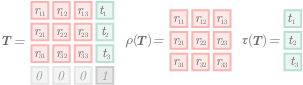
Figure 4: Visualisation of a homogeneous transformation matrix (the derivatives share the form of 𝐓{{\mathbf{T}}}, except will have a 0 instead of a 1 located at 𝐓44{{\mathbf{T}}}_{44}). Where the matrix ρ⁡(𝐓)∈ℝ3×3\rho({{\mathbf{T}}})\in\mathbb{R}^{3\times 3} of green boxes forms the rotation component, and the vector τ⁡(𝐓)∈ℝ3\tau({{\mathbf{T}}})\in\mathbb{R}^{3} of blue boxes form the translation component. The rotation component can be extracted throught the function ρ⁡(⋅):ℝ4×4↦ℝ3×3\rho(\cdot):\mathbb{R}^{4\times 4}\mapsto\mathbb{R}^{3\times 3}, while the translation component can be extracted through the function τ⁡(⋅):ℝ4×4↦ℝ3\tau(\cdot):\mathbb{R}^{4\times 4}\mapsto\mathbb{R}^{3}.

Using the function τ⁡(⋅)\tau(\cdot) which maps the translational component of a 4×44\times 4 matrix to a 33-vector, we can write the translation direction as

𝒗^\displaystyle{\hat{{\bm{v}}}} =τ⁡(d​𝐓𝒕​(d)d​d)\displaystyle=\tau\left(\dfrac{\mathrm{d}{{\mathbf{T}}}_{{\!{\bm{t}}}}(d)}{\mathrm{d}d}\right) (27)

where

𝒗=𝒗^​d˙​(t)\displaystyle{\bm{v}}={\hat{{\bm{v}}}}\dot{d}(t) (28)

The Manipulator Jacobian

Now we can calculate the derivative of an ETS. To find out how the jt​hj^{th} joint affects the end-effector pose, apply the chain rule to (Forward Kinematics)

∂𝐓⁡(𝒒)∂qj\displaystyle\frac{\partial{{{{\mathbf{T}}}}\left({\bm{q}}\right)}}{\partial q_{j}} =∂∂qj​(𝐄1​(η1)​𝐄2​(η2)​…​𝐄M​(ηM))\displaystyle=\frac{\partial}{\partial q_{j}}\left({{\mathbf{E}}}_{1}(\eta_{1}){{\mathbf{E}}}_{2}(\eta_{2})\ldots{{\mathbf{E}}}_{M}(\eta_{M})\right)
=∏i=1μ⁡(j)−1𝐄i​(ηi)​d​𝐄μ⁡(j)​(qj)d​qj​∏i=μ⁡(j)+1M𝐄i​(ηi).\displaystyle=\prod_{i=1}^{\mu(j)-1}{{\mathbf{E}}}_{i}(\eta_{i})\frac{\mathrm{d}{{\mathbf{E}}}_{\mu(j)}(q_{j})}{\mathrm{d}q_{j}}\prod_{i=\mu(j)+1}^{M}{{\mathbf{E}}}_{i}(\eta_{i}). (29)
Refer to caption
Figure 5: Visualisation of the Jacobian 𝐉⁡(𝒒){{\mathbf{J}}}({\bm{q}}) of the Panda serial-link manipulator. Each column describes how the end-effector pose changes due to motion of the corresponding joint. The top three rows 𝐉v{{\mathbf{J}}}_{v} correspond to the linear velocity of the end-effector while the bottom three rows 𝐉ω{{\mathbf{J}_{\!\omega}}} correspond to the angular velocity of the end-effector.

The derivative of the elementary transform with respect to a joint coordinate in (The Manipulator Jacobian) is obtained using one of (20), (21), or (22) for a revolute joint, or one of (24), (25), or (26) for a prismatic joint.

Using (First Derivative of a Pose) with (The Manipulator Jacobian) we can form the angular velocity component of the jt​hj^{th} column of the manipulator Jacobian

𝐉ωj​(𝒒)\displaystyle{{\mathbf{J}}}_{{\!\omega}_{j}}({\bm{q}}) =∨×(ρ(∂𝐓⁡(𝒒)∂qj)ρ(𝐓(𝒒))⊤)\displaystyle=\vee_{\times}\left(\rho\left(\frac{\partial{{{{\mathbf{T}}}}\left({\bm{q}}\right)}}{\partial q_{j}}\right)\rho\left({{{{\mathbf{T}}}}\left({\bm{q}}\right)}\right)^{\top}\right) (30)

and using (11) with (The Manipulator Jacobian), the translational velocity component of the jt​hj^{th} column of the manipulator Jacobian is

𝐉νj​(𝒒)\displaystyle{{\mathbf{J}}}_{{\!\nu}_{j}}({\bm{q}}) =τ⁡(∂𝐓⁡(𝒒)∂qj).\displaystyle=\tau\left(\frac{\partial{{{{\mathbf{T}}}}\left({\bm{q}}\right)}}{\partial q_{j}}\right). (31)
Refer to caption
Figure 6: The two vector representation of a rotation matrix 𝐑∈𝐒𝐎⁡(3){{\mathbf{R}}}\in\mathrm{{\bf SO}(3)}. The rotation matrix 𝐑{{\mathbf{R}}} describes the coordinate frame in terms of three orthogonal vectors 𝒏^{\hat{{\bm{n}}}}, 𝒐^{\hat{{\bm{o}}}}, and 𝒂^{\hat{{\bm{a}}}} which are the axes of the rotated frame expressed in the reference coordinate frame 𝒙^{\hat{{\bm{x}}}}, 𝒚^{\hat{{\bm{y}}}}, and 𝒛^{\hat{{\bm{z}}}}. As shown above, each of the vectors 𝒏^{\hat{{\bm{n}}}}, 𝒐^{\hat{{\bm{o}}}}, and 𝒂^{\hat{{\bm{a}}}} can be calculated using the cross product of the other two.

Stacking the translational and angular velocity components, the jt​hj^{th} column of the manipulator Jacobian becomes

𝐉j​(𝒒)=(𝐉νj​(𝒒)𝐉ωj​(𝒒))∈ℝ6{{\mathbf{J}}}_{j}({\bm{q}})=\begin{pmatrix}{{\mathbf{J}}}_{{\!\nu}_{j}}({\bm{q}})\\ {{\mathbf{J}}}_{{\!\omega}_{j}}({\bm{q}})\end{pmatrix}\in\mathbb{R}^{6} (32)

where the full manipulator Jacobian is

𝐉⁡(𝒒)=(𝐉1​(𝒒)⋯𝐉n​(𝒒))∈ℝ6×n.{{\mathbf{J}}}({\bm{q}})=\begin{pmatrix}{{\mathbf{J}}}_{1}({\bm{q}})&\cdots&{{\mathbf{J}}}_{n}({\bm{q}})\end{pmatrix}\in\mathbb{R}^{6\times n}. (33)

Fast Manipulator Jacobian

We can calculate the manipulator Jacobian using (30) and (31), but has 𝒪⁡(n2)\mathcal{O}(n^{2}) time complexity.

Expanding (30) using (The Manipulator Jacobian) and simplifying using 𝐑𝐑⊤=𝐈{{\mathbf{R}}}{{\mathbf{R}}}^{\top}={{\mathbf{I}}} gives

𝐉ωj​(𝒒)\displaystyle{{\mathbf{J}}}_{{\!\omega}_{j}}({\bm{q}}) =∨×(ρ(𝐓j0)ρ([𝑮^μ⁡(j)])(ρ(0𝐓j)⊤))\displaystyle=\vee_{\times}\bigg(\rho\left({}^{0}{{\mathbf{T}}}_{j}\right)\rho\left(\left[{\hat{{\bm{G}}}}_{\mu(j)}\right]\right)\left(\rho(^{0}{{\mathbf{T}}}_{j})^{\top}\right)\bigg) (34)

where 𝐓j0{}^{0}{{\mathbf{T}}}_{j} represents the transform from the base frame to joint jj as described by (5), and [𝑮^μ⁡(j)][{\hat{{\bm{G}}}}_{\mu(j)}] corresponds to one of the 6 generators from equations (20)-(22) and (24)-(26).

In the case of a prismatic joint, ρ⁡(𝑮^μ⁡(j))\rho({\hat{{\bm{G}}}}_{\mu(j)}) will be a 3×33\times 3 matrix of zeros which results in zero angular velocity. In the case of a revolute joint, the angular velocity is parallel to the axis of joint rotation.

𝐉ωj​(𝒒)\displaystyle{{\mathbf{J}}}_{{\!\omega}_{j}}({\bm{q}}) ={𝒏^jif𝐄m=𝐓𝐑x𝒐^jif𝐄m=𝐓𝐑y𝒂^jif𝐄m=𝐓𝐑z(000)⊤if𝐄m=𝐓𝒕\displaystyle=\left\{\begin{matrix}[l]{\hat{{\bm{n}}}}_{j}&\mbox{if}\ \ {{\mathbf{E}}}_{m}={{\mathbf{T}}}_{{\!{{\mathbf{R}}}}_{x}}\\ {\hat{{\bm{o}}}}_{j}&\mbox{if}\ \ {{\mathbf{E}}}_{m}={{\mathbf{T}}}_{{\!{{\mathbf{R}}}}_{y}}\\ {\hat{{\bm{a}}}}_{j}&\mbox{if}\ \ {{\mathbf{E}}}_{m}={{\mathbf{T}}}_{{\!{{\mathbf{R}}}}_{z}}\\ \begin{pmatrix}0&0&0\end{pmatrix}^{\top}&\mbox{if}\ \ {{\mathbf{E}}}_{m}={{\mathbf{T}}}_{{\!{\bm{t}}}}\\ \end{matrix}\right. (35)

where (𝒏^j𝒐^j𝒂^j)=ρ(0𝐓j)\begin{pmatrix}{\hat{{\bm{n}}}}_{j}&{\hat{{\bm{o}}}}_{j}&{\hat{{\bm{a}}}}_{j}\end{pmatrix}=\rho(^{0}{{\mathbf{T}}}_{j}) as described by the two vector representation displayed in Figure 6.

Expanding (31) using (The Manipulator Jacobian) provides

𝐉νj​(𝒒)\displaystyle{{\mathbf{J}}}_{{\!\nu}_{j}}({\bm{q}}) =τ⁡(𝐓j0​[𝑮^μ⁡(j)]​𝐓ej)\displaystyle=\tau\left({}^{0}{{\mathbf{T}}}_{j}\left[{\hat{{\bm{G}}}}_{\mu(j)}\right]{{}^{j}{{\mathbf{T}}}}_{e}\right) (36)

which reduces to

𝐉νj​(𝒒)\displaystyle{{\mathbf{J}}}_{{\!\nu}_{j}}({\bm{q}}) ={𝒂^j​ye−𝒐^j​zeif𝐄m=𝐓𝐑x𝒏^j​ze−𝒂^j​xeif𝐄m=𝐓𝐑y𝒐^j​xe−𝒚^j​yeif𝐄m=𝐓𝐑z𝒏^jif𝐄m=𝐓𝒕x𝒐^jif𝐄m=𝐓𝒕y𝒂^jif𝐄m=𝐓𝒕z\displaystyle=\left\{\begin{matrix}[l]{\hat{{\bm{a}}}}_{j}y_{e}-{\hat{{\bm{o}}}}_{j}z_{e}&\mbox{if}\ \ {{\mathbf{E}}}_{m}={{\mathbf{T}}}_{{\!{{\mathbf{R}}}}_{x}}\\ {\hat{{\bm{n}}}}_{j}z_{e}-{\hat{{\bm{a}}}}_{j}x_{e}&\mbox{if}\ \ {{\mathbf{E}}}_{m}={{\mathbf{T}}}_{{\!{{\mathbf{R}}}}_{y}}\\ {\hat{{\bm{o}}}}_{j}x_{e}-{\hat{{\bm{y}}}}_{j}y_{e}&\mbox{if}\ \ {{\mathbf{E}}}_{m}={{\mathbf{T}}}_{{\!{{\mathbf{R}}}}_{z}}\\ {\hat{{\bm{n}}}}_{j}&\mbox{if}\ \ {{\mathbf{E}}}_{m}={{\mathbf{T}}}_{{\!{\bm{t}}}_{x}}\\ {\hat{{\bm{o}}}}_{j}&\mbox{if}\ \ {{\mathbf{E}}}_{m}={{\mathbf{T}}}_{{\!{\bm{t}}}_{y}}\\ {\hat{{\bm{a}}}}_{j}&\mbox{if}\ \ {{\mathbf{E}}}_{m}={{\mathbf{T}}}_{{\!{\bm{t}}}_{z}}\\ \end{matrix}\right. (37)

where (𝒏^j𝒐^j𝒂^j)=ρ(0𝐓j)\begin{pmatrix}{\hat{{\bm{n}}}}_{j}&{\hat{{\bm{o}}}}_{j}&{\hat{{\bm{a}}}}_{j}\end{pmatrix}=\rho(^{0}{{\mathbf{T}}}_{j}) and (xeyeze)⊤=τ⁡(𝐓ej)\begin{pmatrix}x_{e}&y_{e}&z_{e}\end{pmatrix}^{\top}=\tau({{}^{j}{{\mathbf{T}}}}_{e}).

This simplification reduces the time complexity of computation of the manipulator Jacobian to 𝒪⁡(n)\mathcal{O}(n).

Manipulator Jacobian
Applications

The manipulator Jacobian is a fundamental tool for robotic control, for the remainder of this article, we detail several applications for the manipulator Jacobian.

Refer to caption
Figure 7: Visualisation of a Panda robot which has been controlled by a position based servoing control scheme utilising resolved-rate motion control. The end-effectors pose has both translated and rotated to reach the desired pose.

Resolved-Rate Motion Control

Resolved-rate motion control (RRMC) is a simple and elegant method to generate straight line motion of the end effector [5]. RRMC is a direct application of the first-order differential equation we generated in (17).

We first re-arrange (17)

𝒒˙=𝐉​(𝒒)−1​𝝂{\dot{{\bm{q}}}}={{{{\mathbf{J}}}}\left({\bm{q}}\right)}^{-1}\ {\bm{\nu}} (38)

which can only be solved when 𝐉⁡(𝒒){{{{\mathbf{J}}}}\left({\bm{q}}\right)} is square (and non-singular), which is when the robot has 6 degrees-of-freedom.

For redundant robots there is no unique solution for (38). Consequently, the most common solution is to use the Moore-Penrose pseudoinverse

𝒒˙=𝐉​(𝒒)+​𝝂{\dot{{\bm{q}}}}={{{{\mathbf{J}}}}\left({\bm{q}}\right)}^{+}\ {\bm{\nu}} (39)

Immediately from this, we can construct a primitive open-loop velocity controller. At each time step we must calculate the manipulator Jacobian 𝐉⁡(𝒒){{{{\mathbf{J}}}}\left({\bm{q}}\right)} which corresponds with the robot’s current configuration qq. Then we set ν\nu to the desired spatial velocity we wish for the end-effector to travel in.

A more useful application of RRMC is to employ it in a closed-loop pose controller which we denote position-based servoing (PBS). Using this method we can get the end-effector to travel in a straight line, in the robot’s task space, towards some desired end-effector pose. The PBS scheme is

𝝂e=k⁡((𝐓e0)−1∙𝐓e∗0){\bm{\nu}}_{e}=k\left((\,{}^{\scriptscriptstyle 0}\!\,{{\mathbf{T}}}_{e})^{-1}\bullet\,{}^{\scriptscriptstyle 0}\!\,{{\mathbf{T}}}_{e^{*}}\right) (40)

where kk is a gain term, 𝐓e0∈𝐒𝐄⁡(3)\,{}^{\scriptscriptstyle 0}\!\,{{\mathbf{T}}}_{e}\in\mathrm{{\bf SE}(3)} is the end-effector pose in the robot’s base frame, 𝐓e∗0∈𝐒𝐄⁡(3)\,{}^{\scriptscriptstyle 0}\!\,{{\mathbf{T}}}_{e^{*}}\in\mathrm{{\bf SE}(3)} is the desired end-effector pose in the robot’s base frame, and ∙\bullet represents composition.

References