跳到论文正文
W Papers独立论文阅读器 arXiv:2207.01761 论文正文 计算阅读时间 · 0%
引用这篇论文根据当前论文元数据生成,正式投稿前建议核对。


License: CC BY 4.0
arXiv:2207.01761v2 [cs.GT] 27 Aug 2023

First Price Auction is 1−1/e21-1/e^{2} Efficient

Yaonan Jin Thanks: Huawei TCS Lab. Work done while the author was a PhD student at Columbia University. Email: jinyaonan@huawei.com    Pinyan Lu Thanks: Shanghai University of Finance and Economics & Huawei TCS Lab. Email: lu.pinyan@mail.shufe.edu.cn
Abstract

We prove that the PoA of First Price Auctions is 1−1/e2≈0.86471-1/e^{2}\approx 0.8647, closing the gap between the best known bounds [0.7430, 0.8689][0.7430,\,0.8689].

1 Introduction

In 1961, Vickrey [Vic61], a Nobel laureate in Economics, initiated auction theory. At the center of his work was the solution concept of Nash equilibrium [Nas50] for auctions as non-cooperative games. This game-theoretical approach has shaped modern auction theory and has a tremendous influence also on other areas in mathematical economics [HR04]. In particular, Vickrey systematically investigated the first-price auction (or its equivalent, the Dutch auction), the most common auction format in real business.

In the first-price auction, the auctioneer (seller) sells an indivisible item to nn potential bidders (buyers). The rule is as simple as it can be: All bidders simultaneously submit bids to the auctioneer (each of which is unknown to the other bidders); the highest bidder wins the item, paying his/her own bid. Simple as the rule is, the bidders’ optimal bidding strategies can be sophisticated. From one bidder’s own perspective, a higher bid means a higher payment on winning but also a better chance of winning. Accordingly, this bidder’s optimal bidding strategy depends on the competitive environment, which in turn is determined by the other bidders’ bidding strategies. This situation is perfectly a non-cooperative game and the standard solution concept is Bayesian Nash equilibrium. To get a better sense, let us show a warm-up example from Vickrey’s original work.

Example 1 ([Vic61]).

Consider two bidders: Alice and Bob have (independent) uniform random values v1,v2∼U⁡[0, 1]v_{1},\,v_{2}\sim U[0,\,1] and respectively bid b1=v12b_{1}=\frac{v_{1}}{2} and b2=v22b_{2}=\frac{v_{2}}{2}. The value distributions and bidding strategies determine the (independent) bid distributions of bidders. In this example, they are (independent) uniform random bids b1,b2∼U⁡[0,12]b_{1},\,b_{2}\sim U[0,\,\frac{1}{2}], whose CDFs are B1​(b)=B2​(b)=min⁡(2​b, 1)B_{1}(b)=B_{2}(b)=\min(2b,\,1). By bidding b≥0b\geq 0, Alice wins with probability min⁡(2​b, 1)\min(2b,\,1) and gains a utility (v1−b)(v_{1}-b) conditioned on winning. Her expected utility is (v1−b)⋅min⁡(2​b, 1)(v_{1}-b)\cdot\min(2b,\,1), which is maximized when b=v12b=\frac{v_{1}}{2}. Thus, her current strategy b1=v12b_{1}=\frac{v_{1}}{2} is optimal. By symmetry, Bob’s current strategy b2=v22b_{2}=\frac{v_{2}}{2} is also optimal. In sum, the above strategy profile (b1,b2)=(v12,v22)(b_{1},\,b_{2})=(\frac{v_{1}}{2},\,\frac{v_{2}}{2}) is an equilibrium, in a sense that no bidder can gain a better utility by deviating from his/her current strategy.

For clarity, let us formalize the model. Each bidder i∈[n]i\in[n] independently draws his/her value from a distribution vi∼Viv_{i}\sim V_{i}. Only with this knowledge and depending on his/her own strategy sis_{i}, bidder ii submits a possibly random bid bi=si​(vi)b_{i}=s_{i}(v_{i}). Then over the randomness of the other bidders’ values 𝒗−i=(vk)k≠i\boldsymbol{v}_{-i}=(v_{k})_{k\neq i} and strategies 𝒔−i={sk}k≠i\boldsymbol{s}_{-i}=\{s_{k}\}_{k\neq i}, bidder ii wins with probability xi​(bi)∈[0, 1]\mathrm{x}_{i}(b_{i})\in[0,\,1] and gains an expected utility ui​(vi,bi)=(vi−bi)⋅xi​(bi)u_{i}(v_{i},\,b_{i})=(v_{i}-b_{i})\cdot\mathrm{x}_{i}(b_{i}).

Definition 1.1 (Equilibria).

A strategy profile 𝒔={si}i∈[n]\boldsymbol{s}=\{s_{i}\}_{i\in[n]} is a Bayesian Nash Equilibrium when: For each bidder i∈[n]i\in[n] and any possible value v∈supp⁡(Vi)v\in\mathrm{supp}(V_{i}), the current strategy si​(v)s_{i}(v) is optimal, namely 𝐄si[ui​(v,si​(v))]≥ui​(v,b)\mathop{{\bf E}\/}_{s_{i}}\big[u_{i}(v,\,s_{i}(v))\big]\geq u_{i}(v,\,b) for any deviation bid b≥0b\geq 0.

Example 1 is special in that bidders have identically distributed values. This symmetric setting is well understood: The first-price auction has a unique Bayesian Nash equilibrium [CH13], which is fully efficient – The bidder with the highest value always wins the item. Instead, the current trend focuses more on the asymmetric setting, where bidders’ values are distinguished by their distributions. Again, let us get a better sense through two concrete examples.

Example 2.

Consider two bidders: Alice has a fixed value v1≡2v_{1}\equiv 2 and always bids s1​(v1)≡1s_{1}(v_{1})\equiv 1. Bob has a uniform random value v2∼U⁡[0, 1]v_{2}\sim U[0,\,1] and truthfully bids his value s2​(v2)=v2s_{2}(v_{2})=v_{2}, namely the distribution B2​(b)=min⁡(b, 1)B_{2}(b)=\min(b,\,1). By bidding b≥0b\geq 0, Alice gains an expected utility (v1−b)⋅min⁡(b, 1)(v_{1}-b)\cdot\min(b,\,1), for which her current strategy s1​(v1)≡1s_{1}(v_{1})\equiv 1 is optimal. Bob cannot gain a positive utility because his value v2∼U⁡[0, 1]v_{2}\sim U[0,\,1] is at most Alice’s bid s1​(v1)≡1s_{1}(v_{1})\equiv 1; thus his current strategy s2​(v2)=v2s_{2}(v_{2})=v_{2} is also optimal. In sum, this strategy profile (s1,s2)(s_{1},s_{2}) is an equilibrium.

Unlike the symmetric setting, this auction game has multiple equilibria. E.g., it is easy to verify that the same strategy s1​(v1)≡1s_{1}(v_{1})\equiv 1 for Alice and a different strategy s~2​(v2)=max⁡(2​v2−1v2, 0)\widetilde{s}_{2}(v_{2})=\max(\frac{2v_{2}-1}{v_{2}},\,0) for Bob (namely the distribution B~2​(b)=12−b\widetilde{B}_{2}(b)=\frac{1}{2-b} for b∈[0, 1]b\in[0,\,1]) are another equilibrium.

Both equilibria (s1,s2)(s_{1},\,s_{2}) and (s1,s~2)(s_{1},\,\widetilde{s}_{2}) given in Example 2 have two features: (i) The strategies s1​(v1)s_{1}(v_{1}), s2​(v2)s_{2}(v_{2}) and s~2​(v2)\widetilde{s}_{2}(v_{2}) are pure strategies – Each of them has no randomness, just the function of a value. (ii) Both equilibria are fully efficient akin to the symmetric setting – Alice always has the highest value ≡2\equiv 2 and always wins the item. However, these are not always the case in the asymmetric setting, such as in the following example, which only slightly modifies Example 2 by changing the fixed value of Alice from 22 to 11.

Example 3.

Consider two bidders: Alice has a fixed value v1≡1v_{1}\equiv 1 and bids s1​(v1)∼B1s_{1}(v_{1})\sim B_{1} following the distribution B1​(b)=14​b−2​exp⁡(4​b−32​b−1)B_{1}(b)=\frac{1}{4b-2}\exp(\frac{4b-3}{2b-1}) for b∈[12,34]b\in[\frac{1}{2},\,\frac{3}{4}]. Bob has a uniform random value v2∼U⁡[0, 1]v_{2}\sim U[0,\,1] and bids s2​(v2)=max⁡(4​v2−14​v2, 0)s_{2}(v_{2})=\max(\frac{4v_{2}-1}{4v_{2}},\,0), namely the distribution B2​(b)=14−4​bB_{2}(b)=\frac{1}{4-4b} for b∈[0,34]b\in[0,\,\frac{3}{4}]. By bidding b≥0b\geq 0, Alice gains an expected utility (v1−b)⋅B2​(b)(v_{1}-b)\cdot B_{2}(b), which is maximized =14=\frac{1}{4} anywhere between b∈[0,34]b\in[0,\,\frac{3}{4}], so her current strategy s1​(v1)∼B1s_{1}(v_{1})\sim B_{1} is optimal. Using elementary algebra, we can check that Bob’s current strategy s2​(v2)=max⁡(4​v2−14​v2, 0)s_{2}(v_{2})=\max(\frac{4v_{2}-1}{4v_{2}},\,0) also is optimal. In sum, this strategy profile (s1,s2)(s_{1},s_{2}) is an equilibrium.

In Example 3: Alice has a mixed strategy – A fixed value v1≡1v_{1}\equiv 1 but a random bid s1​(v1)∼B1s_{1}(v_{1})\sim B_{1}. Furthermore, the equilibrium (s1,s2)(s_{1},\,s_{2}) is not fully efficient. E.g., with a value v2=34v_{2}=\frac{3}{4}, although not the highest value <v1≡1<v_{1}\equiv 1, Bob bids s2​(v2)=23s_{2}(v_{2})=\frac{2}{3} and wins with probability B1​(23)=32​e≈0.5518B_{1}(\frac{2}{3})=\frac{3}{2e}\approx 0.5518. Indeed, Example 3 has infinite equilibria, among which the given one (s1,s2)(s_{1},s_{2}) has the relatively “simplest” format. But none of those equilibria is a pure equilibrium or is fully efficient, despite that Example 3 is only a minor modification of Example 2.

From the above examples, we observe that Bayesian Nash equilibria can be very complicated and sensitive to the value distributions, despite the intrinsic simple rule of the first-price auction. After an extensive study for more than 60 years, the first-price auction and its equilibria remain the centerpiece of modern auction theory and have promoted a rich literature; see [SZ90, Leb06, Leb96, Leb99, MR00a, MR00b, JSSZ02, MR03, HKMN11, CH13, ST13, Syr14, HHT14, FLN16, HTW18, WSZ20, FGH+21] etc. These efforts are justifiable since the study of the first-price auction and its equilibria is both theoretically challenging and practically important.

Among various aspects of the first-price auction, efficiency at equilibria is of primary interest. In economics, efficiency measures to what extent a resource can be allocated to the persons who value it the most, thus maximizing the social welfare, particularly in a competitive environment. As shown above (Example 3), the first-price auction generally is not fully efficient at an equilibrium: The winner has the highest bid but possibly not the highest value; this crucially depends on both (i) the instance 𝑽\boldsymbol{V} itself and (ii) which Bayesian Nash equilibrium 𝒔∈𝔹​ℕ​𝔼​(𝑽)\boldsymbol{s}\in\mathbb{BNE}(\boldsymbol{V}) it falls into. Earlier works in economics focus on (generalizing) the conditions for the value distribution 𝑽={Vi}i∈[n]\boldsymbol{V}=\{V_{i}\}_{i\in[n]} that guarantee the full efficiency.

However, the quality of (in)efficiency should not be all-or-nothing. E.g., when the highest value is 11, a value-0.990.99 bidder versus a value-0.010.01 bidder is very different, although neither of them is fully efficient. Towards a quantitative analysis, Koutsoupias and Papadimitriou introduced a new measure on the efficiency degradation under selfish behaviors, the Price of Anarchy [KP99] (which is an analog of the “approximation ratio” in theoretical computer science). For the first-price auction, denote by 𝖮𝖯𝖳⁡(𝑽){\sf OPT}(\boldsymbol{V}) the expected optimal social welfare from an instance 𝑽\boldsymbol{V}, and by 𝖥𝖯𝖠⁡(𝑽,𝒔){\sf FPA}(\boldsymbol{V},\,\boldsymbol{s}) the expected social welfare at an equilibrium 𝒔∈𝔹​ℕ​𝔼​(𝑽)\boldsymbol{s}\in\mathbb{BNE}(\boldsymbol{V}), then the Price of Anarchy is defined to be the minimum possible ratio, as follows.

Definition 1.2 (Price of Anarchy).

Regarding First Price Auctions, the Price of Anarchy is given by

𝖯𝗈𝖠:=inf{𝖥𝖯𝖠⁡(𝑽,𝒔)𝖮𝖯𝖳⁡(𝑽)|𝒔∈𝔹​ℕ​𝔼​(𝑽)​and​𝖮𝖯𝖳​(𝑽)<+∞}.{\sf PoA}~:=~\inf\bigg\{\,\frac{{\sf FPA}(\boldsymbol{V},\,\boldsymbol{s})}{{\sf OPT}(\boldsymbol{V})}\,\,\bigg|\,\bigg.\,\boldsymbol{s}\in\mathbb{BNE}(\boldsymbol{V})~\text{and}~{\sf OPT}(\boldsymbol{V})<+\infty\,\bigg\}.

The Price of Anarchy is bounded between [0, 1][0,\,1]. Namely, a larger ratio means a higher efficiency and the =1=1 ratio means the full efficiency. For the first-price auction, Syrgkanis and Tardos first proved that the PoA is at least 1−1/e≈0.63211-1/e\approx 0.6321 [ST13]. Later, Hoy, Taggart and Wang derived an improved lower bound of ≈0.7430\approx 0.7430 [HTW18]. On the other hand, Hartline, Hoy and Taggart gave a concrete instance of ratio ≈0.8689\approx 0.8689 [HHT14], which remains the best known upper bound.

Despite the prevalence of the first-price auction and much effort in studying its efficiency, there has been a persistent gap in the state of the art. In the current paper, we will completely solve this long-standing open problem.

Theorem 1 (Tight PoA).

The Price of Anarchy in First Price Auctions is 1−1/e2≈0.86471-1/e^{2}\approx 0.8647.

Remarkably, neither the best known lower bound ≈0.7430\approx 0.7430 nor the upper bound ≈0.8689\approx 0.8689 is tight; we close the gap by improving both of them. Our tight bound 1−1/e2≈0.86471-1/e^{2}\approx 0.8647 not only is a mathematically elegant result but has further implications in real business since it is fairly close to 11. Namely, at any equilibrium, the efficiency degradation in the first-price auction is small, no worse than 13.53%, which might be acceptable given other merits of the first-price auction.

En route to the tight PoA, we obtain many new important perspectives, characterizations, and properties of equilibria in the first-price auction. These might be of independent interest and find applications in the future study of other aspects of the first-price auction, e.g., the complexity of computing equilibria. Beyond the first-price auction, our overall approach is general enough and might help determine the Price of Anarchy in other auctions.

1.1 Technical overview

This subsection sketches our high-level proof ideas. To ease the readability, some descriptions are roughly accurate but not perfectly, and most technical details are deferred to Sections 2, 3, 4, 5 and 6. Our approach is very different from the prior works [ST13, HTW18], which mainly adopt the smoothness techniques or an extension. More concretely, we employ a first principle approach that directly characterizes the worst-case instance and the worst-case Bayesian Nash equilibrium regarding the definition of the Price of Anarchy. To this end, we step by step narrow down the search space of the worst case by proving more and more necessary conditions it must satisfy. Finally, we capture the exact worst case and thus derive the tight PoA bound.

Changing the viewpoints (Section 2)

Regarding the PoA definition, we need to prove that the auction social welfare 𝖥𝖯𝖠⁡(𝑽,𝒔){\sf FPA}(\boldsymbol{V},\,\boldsymbol{s}) is within a certain ratio of the optimal social welfare 𝖮𝖯𝖳⁡(𝑽){\sf OPT}(\boldsymbol{V}), given any value distribution 𝑽={Vi}i∈[n]\boldsymbol{V}=\{V_{i}\}_{i\in[n]} and any equilibrium thereof 𝒔={si}i∈[n]\boldsymbol{s}=\{s_{i}\}_{i\in[n]}.

Two difficulties emerge immediately: (i) One value distribution 𝑽∈𝕍\boldsymbol{V}\in\mathbb{V} generally has multiple or even infinite equilibria. (ii) One equilibrium 𝒔∈𝔹​ℕ​𝔼​(𝑽)\boldsymbol{s}\in\mathbb{BNE}(\boldsymbol{V}) generally has no analytic solution; even an efficient algorithm for computing (approximate) equilibria from value distributions is unknown.

To the rescue, instead of the original value-strategy representation (𝑽,𝒔)∈𝕍×𝔹​ℕ​𝔼(\boldsymbol{V},\,\boldsymbol{s})\in\mathbb{V}\times\mathbb{BNE} of equilibria, we use another representation, the bid distributions 𝑩⁡(𝑽,𝒔)\boldsymbol{B}(\boldsymbol{V},\,\boldsymbol{s}) resulted from equilibria. These two representations and their relationship are demonstrated in Figure 1. Given one equilibrium bid distribution 𝑩⁡(𝑽,𝒔)={Bi}i∈[n]\boldsymbol{B}(\boldsymbol{V},\,\boldsymbol{s})=\{B_{i}\}_{i\in[n]}: (i) One equilibrium (𝑽,𝒔)∈𝕍×𝔹​ℕ​𝔼(\boldsymbol{V},\,\boldsymbol{s})\in\mathbb{V}\times\mathbb{BNE} is uniquely determined. (ii) The reconstruction of the (𝑽,𝒔)(\boldsymbol{V},\,\boldsymbol{s}) essentially has an analytic solution, through the bid-to-value mappings φi​(b):=b+(∑k≠iBk′​(b)/Bk​(b))−1\varphi_{i}(b):=b+(\sum_{k\neq i}B^{\prime}_{k}(b)/B_{k}(b))^{-1} that are almost the inverse functions of the strategies 𝒔={si}i∈[n]\boldsymbol{s}=\{s_{i}\}_{i\in[n]}.11 1 Although the mapping formulas φi​(b)=b+(∑k≠iBk′​(b)/Bk​(b))−1\varphi_{i}(b)=b+(\sum_{k\neq i}B^{\prime}_{k}(b)/B_{k}(b))^{-1} are previously known, NO prior work takes ANY further step. Even this structure result is unknown: “One (valid) bid distribution 𝑩∈𝔹𝗏𝖺𝗅𝗂𝖽\boldsymbol{B}\in\mathbb{B}_{\sf valid} backward uniquely determines the underlying value-strategy tuple (𝑽,𝒔)∈𝕍×𝔹​ℕ​𝔼(\boldsymbol{V},\,\boldsymbol{s})\in\mathbb{V}\times\mathbb{BNE}”; let alone techniques towards the tight 𝖯𝗈𝖠=1−1/e2{\sf PoA}=1-1/e^{2}. These mitigate the above two difficulties.

In sum, there is a bijection between the space of equilibria 𝕍×𝔹​ℕ​𝔼∋(𝑽,𝒔)\mathbb{V}\times\mathbb{BNE}\ni(\boldsymbol{V},\,\boldsymbol{s}) and the space of equilibrium bid distributions {𝑩⁡(𝑽,𝒔)}\{\boldsymbol{B}(\boldsymbol{V},\,\boldsymbol{s})\}. Further, the new representation {𝑩⁡(𝑽,𝒔)}\{\boldsymbol{B}(\boldsymbol{V},\,\boldsymbol{s})\} is mathematically equivalent but technically easier – this is one infinite set instead of the Cartesian product 𝕍×𝔹​ℕ​𝔼\mathbb{V}\times\mathbb{BNE} of two infinite sets – showing an avenue towards the tight PoA. (Later in Sections 2, 3, 4, 5 and 6, we will see more advantages.)

Space 𝕍\mathbb{V}Space 𝔹𝗏𝖺𝗅𝗂𝖽\mathbb{B}_{\sf valid}𝑽\boldsymbol{V}𝑩\boldsymbol{B}𝑩¯\overline{\boldsymbol{B}}𝑩^\widehat{\boldsymbol{B}}𝑽~\widetilde{\boldsymbol{V}}𝑩~\widetilde{\boldsymbol{B}}𝒔∈𝔹​ℕ​𝔼​(𝑽)\boldsymbol{s}\in\mathbb{BNE}(\boldsymbol{V})𝒔¯∈𝔹​ℕ​𝔼​(𝑽)\overline{\boldsymbol{s}}\in\mathbb{BNE}(\boldsymbol{V})𝒔^∈𝔹​ℕ​𝔼​(𝑽)\widehat{\boldsymbol{s}}\in\mathbb{BNE}(\boldsymbol{V})𝒔~∈𝔹​ℕ​𝔼​(𝑽)\widetilde{\boldsymbol{s}}\in\mathbb{BNE}(\boldsymbol{V})
(a) Forward direction: 𝕍×𝔹​ℕ​𝔼↦𝔹𝗏𝖺𝗅𝗂𝖽\mathbb{V}\times\mathbb{BNE}\mapsto\mathbb{B}_{\sf valid}
Space 𝕍×𝔹​ℕ​𝔼\mathbb{V}\times\mathbb{BNE}Space 𝔹𝗏𝖺𝗅𝗂𝖽\mathbb{B}_{\sf valid}(𝑽,𝒔)(\boldsymbol{V},\,\boldsymbol{s})𝑩\boldsymbol{B}(𝑽,𝒔¯)(\boldsymbol{V},\,\overline{\boldsymbol{s}})𝑩¯\overline{\boldsymbol{B}}(𝑽,𝒔^)(\boldsymbol{V},\,\widehat{\boldsymbol{s}})𝑩^\widehat{\boldsymbol{B}}(𝑽~,𝒔~)(\widetilde{\boldsymbol{V}},\,\widetilde{\boldsymbol{s}})𝑩~\widetilde{\boldsymbol{B}}
(b) Inverse direction: 𝔹𝗏𝖺𝗅𝗂𝖽↦𝕍×𝔹​ℕ​𝔼\mathbb{B}_{\sf valid}\mapsto\mathbb{V}\times\mathbb{BNE}
Figure 1: Diagram of the two representations of equilibrium, (i) the value-strategy representation (𝑽,𝒔)∈𝕍×𝔹​ℕ​𝔼(\boldsymbol{V},\,\boldsymbol{s})\in\mathbb{V}\times\mathbb{BNE} versus (ii) the bid distribution representation 𝑩=𝑩⁡(𝑽,𝒔)∈𝔹𝗏𝖺𝗅𝗂𝖽\boldsymbol{B}=\boldsymbol{B}(\boldsymbol{V},\,\boldsymbol{s})\in\mathbb{B}_{\sf valid}. One value distribution 𝑽\boldsymbol{V} has multiple or even infinite equilibria 𝒔∈𝔹​ℕ​𝔼​(𝑽)\boldsymbol{s}\in\mathbb{BNE}(\boldsymbol{V}); each equilibrium induces one valid bid distribution 𝑩=𝑩⁡(𝑽,𝒔)∈𝔹𝗏𝖺𝗅𝗂𝖽\boldsymbol{B}=\boldsymbol{B}(\boldsymbol{V},\,\boldsymbol{s})\in\mathbb{B}_{\sf valid}. Backward, the 𝑩\boldsymbol{B} determines the underlying tuple (𝑽,𝒔)∈𝕍×𝔹​ℕ​𝔼(\boldsymbol{V},\,\boldsymbol{s})\in\mathbb{V}\times\mathbb{BNE} via the bid-to-value mappings 𝝋\boldsymbol{\varphi}. Hence, there is a bijection between the two spaces 𝕍×𝔹​ℕ​𝔼\mathbb{V}\times\mathbb{BNE} and 𝔹𝗏𝖺𝗅𝗂𝖽\mathbb{B}_{\sf valid}.

Nonetheless, there is no free lunch. The new representation has two drawbacks. (i) Unlike that any value distribution 𝑽∈𝕍\boldsymbol{V}\in\mathbb{V} must be feasible since the existence of an equilibrium 𝒔∈𝔹​ℕ​𝔼​(𝑽)\boldsymbol{s}\in\mathbb{BNE}(\boldsymbol{V}) is promised [Leb96],22 2 This existence result requires suitable tie-breaking rules in the first-price auction; see Section 2 for more details. a generic bid distribution 𝑩\boldsymbol{B} not necessarily induces an equilibrium. To remedy this issue, we introduce the notion of validity, which almost refers to monotonicity of the bid-to-value mappings 𝝋={φi}i∈[n]\boldsymbol{\varphi}=\{\varphi_{i}\}_{i\in[n]}. In addition, (ii) a mapping φi\varphi_{i} is undefined at a singular point where the equilibrium bid distribution BiB_{i} of that bidder i∈[n]i\in[n] has a probability mass, which must be handled separately. Luckily, such probability masses are possible only at the left endpoint of the distribution’s support. So, we further consider the conditional value distribution PP given one’s bid being at the left endpoint. Indeed, the concept of validity refers to a tuple (𝑩,P)(\boldsymbol{B},\,P) of equilibrium bid distributions and a conditional value distribution.

More rigorously, our new representation considers all the valid tuples/instances (𝑩,P)∈𝔹𝗏𝖺𝗅𝗂𝖽(\boldsymbol{B},\,P)\in\mathbb{B}_{\sf valid}. Here, the valid distributions 𝑩\boldsymbol{B} can be replaced with the increasing bid-to-value mappings 𝝋\boldsymbol{\varphi}: One determines the other and vice versa (Lemma 3.4). More importantly, monotonicity of the mappings 𝝋\boldsymbol{\varphi} gives a strong geometric intuition, making the third representation (𝝋,P)(\boldsymbol{\varphi},\,P) of equilibrium more convenient for our later use. In particular, in what follows, the figures of the mappings 𝝋={φi}i∈[n]\boldsymbol{\varphi}=\{\varphi_{i}\}_{i\in[n]} play the role of visual demonstrations, i.e., horizontal bid axes and vertical value axes, where each mapping φi\varphi_{i} denotes one bidder i∈[n]i\in[n].

The worst-case instance (Section 6)

Our overall approach is to reduce any given instance to the worst-case instance step by step. Thus, it is helpful to describe the worst case in advance, which explains why we design those reductions since our target is very specific.

Refer to caption
Figure 2: The worst case instance H⊗{Ln}⊗nH\otimes\{\sqrt[n]{L}\}^{\otimes n}. Bidder HH has a fixed high value φH​(b)≡1\varphi_{H}(b)\equiv 1 for b∈[0, 1−4/e2]b\in[0,\,1-4/e^{2}] and each bidder LL has the (parametric) bid-to-value mapping φL​(1−t2⋅e2−2​t)=1−t⋅e2−2​t\varphi_{L}(1-t^{2}\cdot e^{2-2t})=1-t\cdot e^{2-2t} for t∈[1, 2]t\in[1,\,2].

The worst case has n+1n+1 bidders, one bidder HH with a fixed high value vH≡1v_{H}\equiv 1 and sufficiently many n≫1n\gg 1 identical low-value bidders {Ln}⊗n\{\sqrt[n]{L}\}^{\otimes n}. Among the low-value bidders, the highest value vL∼VLv_{L}\sim V_{L} is distributed following the parametric equation VL​(1−t⋅e2−2​t)=4/t2⋅e2​t−4V_{L}(1-t\cdot e^{2-2t})=4/t^{2}\cdot e^{2t-4} for t∈[1, 2]t\in[1,\,2], over the value support vL∈supp⁡(VL)=[0, 1−2/e2]v_{L}\in\mathrm{supp}(V_{L})=[0,\,1-2/e^{2}]. See Figure 2 for a visual aid, based on the bid-to-value mappings φH⊗{φL}⊗n\varphi_{H}\otimes\{\varphi_{L}\}^{\otimes n}.

The equilibrium strategies sH⊗{sL}⊗ns_{H}\otimes\{s_{L}\}^{\otimes n} and the bid distributions H⊗{Ln}⊗nH\otimes\{\sqrt[n]{L}\}^{\otimes n} are less important for understanding our approach;33 3 [HHT14] “just” considered a reasonable instance H⁡(b)=b/λH(b)=\sqrt{b/\lambda} and L⁡(b)=1−λ1−bL(b)=\frac{1-\lambda}{1-b} for λ=0.57\lambda=0.57, but neither gave argument/evidence for “worstness” of the instance family H⊗{Ln}⊗nH\otimes\{\sqrt[n]{L}\}^{\otimes n}, nor searched the worst case (H∗,λ∗)(H^{*},\,\lambda^{*}). In contrast, our contributions are twofold: (primary) “worstness” of this family; (secondary) the nontrivial worst case b=1−4​H∗⋅e2−4​H∗b=1-{4H^{*}}\cdot{e^{2-4\sqrt{H^{*}}}} and L∗​(b)=1−λ∗1−bL^{*}(b)=\frac{1-\lambda^{*}}{1-b} for λ∗=1−4/e2\lambda^{*}=1-4/e^{2}. In this family, the PoA is less sensitive to different instances, hence two numerically close bounds 0.86890.8689 versus 0.86470.8647. we will show in Section 6 how to deduce them and the tight PoA =1−1/e2=1-1/e^{2}. The parametric equation VLV_{L} also is less important, being included just for completeness.

In contrast, the point is the underlying structure: The bidder HH always contributes the optimal social welfare ≡1\equiv 1. The low-value bidders {Ln}⊗n\{\sqrt[n]{L}\}^{\otimes n} individually have negligible effects (the winning probabilities etc) but collectively make the auction game less efficient.

We are inspired by the instance due to Hartline, Hoy and Taggart [HHT14], which has the same H⊗{Ln}⊗nH\otimes\{\sqrt[n]{L}\}^{\otimes n} structure. Our construction differs from theirs in the concrete distributions, hence a slightly worse PoA of 1−1/e2≈0.86471-1/e^{2}\approx 0.8647 in comparison with their ratio of ≈0.8689\approx 0.8689 (Footnote 3).

The pseudo instances (Section 3.1) and (Section 4.3)

Rigorously, the worst case H⊗{Ln}⊗nH\otimes\{\sqrt[n]{L}\}^{\otimes n} for n≫1n\gg 1 described above is not a specific instance, but a sequence of instances with the limit n→+∞n\to+\infty being the worst case. This incurs some notational inconvenience. When such issues occur in real/complex analysis, the standard method is to add the infinite point(s) to the space of the real/complex numbers, making the space more complete. In the same spirit, we introduce the notion of pseudo bidders and pseudo instances (Definition 3.1), thus including the above limit to our search space.

Refer to caption
(a) The input non collapsed mappings 𝝋\boldsymbol{\varphi}
Refer to caption
(b) The output collapsed mappings 𝝋~\widetilde{\boldsymbol{\varphi}}
Figure 3: The Collapse reduction. When a specific bidder i∈[n]i\in[n] has a fixed high value φi​(b)≡vi≥max⁡{φk​(b):k≠i}\varphi_{i}(b)\equiv v_{i}\geq\max\{\varphi_{k}(b):k\neq i\} over the bid support b∈[γ,λ]b\in[\gamma,\,\lambda], the Collapse reduction transforms this instance 𝑩=Bi⊗𝑩−i\boldsymbol{B}=B_{i}\otimes\boldsymbol{B}_{-i} to a two-bidder pseudo instance Bi⊗L~B_{i}\otimes\widetilde{L} that yields a worse-or-equal PoA.

In our extended language, the worst case has a succinct format: one high-value bidder HH and one pseudo bidder LL, namely a two-bidder pseudo instance (Figure 2). Beyond notational brevity, the notion of pseudo bidders/instances also simplifies our proof in several places.

This extension does not hurt our proof, given that pseudo instances are only considered in the lower-bound analysis. Precisely, we show that even the worst case in the extended search space has the PoA ≥1−1/e2\geq 1-1/e^{2}, implying a lower bound of 1−1/e21-1/e^{2} for the original problem. In addition, the upper-bound analysis leverages the above instance sequence H⊗{Ln}⊗nH\otimes\{\sqrt[n]{L}\}^{\otimes n}. Precisely, we show that when the n≫1n\gg 1 is sufficiently large, the PoA can be arbitrarily close to 1−1/e21-1/e^{2}. As a combination, the tight PoA in Theorem 1 gets established.

Another related thing is the reduction. As Figures 3a and 3b show, when a specific bidder i∈[n]i\in[n] has a fixed high value φi​(b)≡vi≥max⁡{φk​(b):k≠i}\varphi_{i}(b)\equiv v_{i}\geq\max\{\varphi_{k}(b):k\neq i\} over the bid support b∈[γ,λ]b\in[\gamma,\,\lambda], the reduction can replace all the other bidders {Bk}k≠i\{B_{k}\}_{k\neq i} by one pseudo bidder L~\widetilde{L}, resulting in a two-bidder pseudo instance Bi⊗L~B_{i}\otimes\widetilde{L} that has a worse-or-equal PoA. (I.e, whether before or after the reduction, the optimal social welfare is the bidder ii’s fixed high value ≡vi\equiv v_{i}. Moreover, it turns out that the auction social welfare can only decrease.) Such a two-bidder pseudo instance Bi⊗L~B_{i}\otimes\widetilde{L} will be easy to handle since it has the same shape as the worst case H⊗LH\otimes L.

In sum, the remaining task is to transform every valid instance ∈𝔹𝗏𝖺𝗅𝗂𝖽\in\mathbb{B}_{\sf valid} into a specific instance that the Collapse reduction can work on, i.e., an instance that has one fixed-high-value bidder.

(Section 3.4): Hierarchizing the bidders

Refer to caption
(a) The input increasing mappings 𝝋\boldsymbol{\varphi}
Refer to caption
(b) The output layered mappings 𝝋~\widetilde{\boldsymbol{\varphi}}
Figure 4: The Layer reduction. Each color corresponds to a bidder. After the reduction, the bidders are ordered. For example, the red bidder is the highest bidder.

To transform a given instance into the worst case, we shall identify one special high-value bidder H∈[n]H\in[n] and “derandomize” his/her value, i.e., making the bid-to-value mapping a constant function φH​(b)≡vH\varphi_{H}(b)\equiv v_{H}. (If so, upon scaling, we can normalize this fixed value vH=1v_{H}=1.) But it is even unclear which bidder i∈[n]i\in[n] should be the candidate: The highest-value bidder argmax{φi​(b):i∈[n]}\mathop{\mathrm{argmax}}\{\varphi_{i}(b):i\in[n]\} at different bids b∈[γ,λ]b\in[\gamma,\,\lambda] can be different. More concretely, consider the example in Figure 4a, the highest-value bidder is the red bidder B1B_{1} initially for small bids, but changes to the blue bidder B2B_{2} later for large bids.

We can segment the bid-to-value mappings into pieces and rearrange them, in a sense of Figure 4b, making them ordered point-wise φ~1​(b)≥⋯≥φ~n​(b)\widetilde{\varphi}_{1}(b)\geq\dots\geq\widetilde{\varphi}_{n}(b). Then, the candidate high-value bidder clearly is the index-11 bidder B~1\widetilde{B}_{1} (i.e., the red one in Figure 4b). We call this reduction .

Under the reduction, the auction/optimal social welfares FPA and OPT each remain the same, so the PoA is invariant. This proof is not that technically involved, once we formalize the reduction. However, without switching our viewpoint to the bid-to-value mappings 𝝋={φi}i∈[n]\boldsymbol{\varphi}=\{\varphi_{i}\}_{i\in[n]}, even describing this reduction seems difficult.

In sum, we narrow down the search space to the “layered” instances and the remaining task to address the candidate high-value bidder B1B_{1}, particularly derandomizing his/her value φ1​(b)≡v1\varphi_{1}(b)\equiv v_{1}.

and (Sections 3.2 and 3.3): Two simplifications

Refer to caption
(a) The input increasing mappings 𝝋\boldsymbol{\varphi}
Refer to caption
(b) The output discretized/translated mappings 𝝋~\widetilde{\boldsymbol{\varphi}}
Figure 5: The Discretize and Translate reductions

Our main reduction is an iterative algorithm; thus it is convenient to work with bounded discrete instances, for which the main reduction will terminate in finite iterations. Such an idea appears in many prior works [CGL14, AHN+19, JLTX20, JLQ+19, JJLZ21], and the proof plan is twofold: (i) For any bounded discrete instance, the PoA is at least 1−1/e21-1/e^{2}. (ii) For any valid instance, there exists a bounded discrete instance approximating the PoA, up to an arbitrary but fixed error ε>0\varepsilon>0. As a combination, the PoA for any valid instance is at least 1−1/e21-1/e^{2}.

However, our discretization scheme is subtle. First, we cannot discretize the valid bid distributions 𝑩\boldsymbol{B} given that they must be continuous everywhere except the left endpoint of the bid support. Second, we cannot discretize the value distributions and the strategies (𝑽,𝒔)(\boldsymbol{V},\,\boldsymbol{s}). Although bounded discrete value distributions 𝑽~\widetilde{\boldsymbol{V}} that well approximate the given ones 𝑽\boldsymbol{V} are trivial, it is unclear how to obtain desirable strategies 𝒔~∈𝔹​ℕ​𝔼​(𝑽~)\widetilde{\boldsymbol{s}}\in\mathbb{BNE}(\widetilde{\boldsymbol{V}}): No algorithm for computing equilibria from value distributions is available. Also, with modified value distributions, even the existence of 𝒔~∈𝔹​ℕ​𝔼​(𝑽~)\widetilde{\boldsymbol{s}}\in\mathbb{BNE}(\widetilde{\boldsymbol{V}}) that is “close enough” to the given equilibrium 𝒔∈𝔹​ℕ​𝔼​(𝑽)\boldsymbol{s}\in\mathbb{BNE}(\boldsymbol{V}) is doubtful.

We circumvent these issues by discretizing the bid-to-value mappings 𝝋\boldsymbol{\varphi} instead (Figure 5), i.e., approximating them through piecewise constant functions 𝝋~\widetilde{\boldsymbol{\varphi}}.44 4 In real analysis, for various purposes, piecewise constant functions (a.k.a. simple functions) are widely used as approximations to general functions. The benefits are threefold: (i) The valid bid distributions 𝑩~\widetilde{\boldsymbol{B}}, the value distributions 𝑽~\widetilde{\boldsymbol{V}}, and the equilibrium strategies 𝒔~∈𝔹​ℕ​𝔼​(𝑽~)\widetilde{\boldsymbol{s}}\in\mathbb{BNE}(\widetilde{\boldsymbol{V}}) can be reconstructed from the new mappings 𝝋~\widetilde{\boldsymbol{\varphi}}, through analytic expressions. (ii) The piecewise constancy of the new mappings 𝝋~\widetilde{\boldsymbol{\varphi}} makes the value distribution 𝑽~\widetilde{\boldsymbol{V}} bounded and discrete. (iii) More importantly, we are able to obtain a sequence of piecewise constant mappings {𝝋~}\{\widetilde{\boldsymbol{\varphi}}\} that pointwise converge to the given ones 𝝋\boldsymbol{\varphi}. The corresponding {𝑩~}\{\widetilde{\boldsymbol{B}}\}, {𝑽~}\{\widetilde{\boldsymbol{V}}\}, and {𝒔~}\{\widetilde{\boldsymbol{s}}\} can be arbitrarily close to the given 𝑩\boldsymbol{B},  𝑽\boldsymbol{V}, and 𝒔\boldsymbol{s}, approximating the PoA up to any fixed error ε>0\varepsilon>0. This exactly implements the second part of our proof plan.

Afterward, the reduction further vanishes the lowest bid, through shifting both the value space and the bid space by the same distance of −γ-\gamma (Fig. 5). As a consequence, both the auction/optimal social welfares decrease by an amount of γ\gamma, giving a worse-or-equal PoA.

In sum, we can focus on piecewise constant and increasing mappings 𝝋\boldsymbol{\varphi} over a bounded support b∈[0,λ]b\in[0,\,\lambda], together with the conditional value PP given the nil bid b=0b=0 (i.e., the left endpoint).

and (Sections 3.5 and 4.2): Dealing with the probability masses

Now we address the probability masses and the conditional value PP. (This is the only information that cannot be reconstructed from the bid-to-value mappings 𝝋\boldsymbol{\varphi} and must be handled separately.) Our main observation is (Lemma 2.16) that at most one bidder can have a nontrivial conditional value PP, who will be called the monopolist HH. (After the reduction, this monopolist HH will be the high-value bidder; cf. Figure 4.) That is why we can use a single conditional value PP, instead of nn values akin to the distributions 𝑽\boldsymbol{V} or 𝑩\boldsymbol{B}. Moreover, following the monotonicity, this value PP is supported on [0,φH​(0)][0,\varphi_{H}(0)].

The reduction derandomizes the conditional value by moving all the probabilities to either P≡0P\equiv 0 or P≡φH​(0)P\equiv\varphi_{H}(0). Namely, this is a win-win reduction, in a sense that at least one of the two possibilities P≡0P\equiv 0 and P≡φH​(0)P\equiv\varphi_{H}(0) induces a worse-or-equal PoA than the given instance. Later, such win-win reductions also appear in several other places.

Further, the reduction totally determines the conditional value P≡φH​(0)P\equiv\varphi_{H}(0) by eliminating the other possibility. This reduction modifies both the conditional value PP and the mappings 𝝋\boldsymbol{\varphi}, thus far more complicated than the reduction, which only modifies the PP.55 5 For very technical reasons, we should not unify and into a single reduction (cf. Sections 3 and 4).

In conclusion, we can drop the notation PP hereafter: Just the piecewise constant and increasing mappings 𝝋\boldsymbol{\varphi} are enough to describe the entire instance and the reductions on it.

10 and (Sections 4.4 and 4.5): The main reductions

Our main reduction aims to reduce the number of pieces of the high-value bidder HH’s mapping φH\varphi_{H}. (After the reduction, this mapping has finite many pieces. In particular, the one in the worst-case instance has one single piece (Figure 2), namely a constant mapping.) To this end, we look at the first jump point of this mapping φH\varphi_{H}. Furthermore, we distinguish two types of jumps, pseudo jumps versus real jumps, and adopt two different reductions respectively.

For a 4.4 (), the after-jump parts of all mappings 𝝋\boldsymbol{\varphi} are universally higher than the before-jump parts, so the entire instance naturally divides into the left-lower part versus the right-upper part ( and ). We prove that at least one part induces a worse-or-equal PoA than the given instance.66 6 In particular, for the right-upper part, we reapply the reduction to make the bid space start from 00. This is another win-win reduction and will be called 10.

For a 4.5 (), the after-jump parts (of some mappings) still interlace with the before-jump parts. We would modify the first two pieces of the high-value mapping φH\varphi_{H} to reduce the number of pieces by one. I.e., we either ascend the first piece to the value of the second piece () or descend the second piece to the value of the first piece (). We show that at least one modification gives a worse-or-equal PoA than the given instance. This is again a win-win reduction and will be called .

To conclude, whether a 4.4 or a 4.5, we obtain a new instance that (i) has a worse-or-equal PoA and (ii) the high-value mapping φH\varphi_{H} has one fewer piece. Clearly, we can iterate the entire process until a constant mapping φH​(b)≡vH\varphi_{H}(b)\equiv v_{H}, i.e., one single piece. Then, the reduction can replace all the other bidders {Bk}k≠H\{B_{k}\}_{k\neq H} by one pseudo bidder LL, hence a two-bidder pseudo instance H⊗LH\otimes L that has the same shape as the worst case (Figure 3), as desired.

We stress again that the above description is greatly simplified and thus just roughly accurate – The high-level idea is delivered, but most technical details are hidden.

Solving the functional optimization (Section 5)

After the above reductions, we get a nice-looking instance: (i) one bidder HH with a fixed high value φH​(b)≡vH\varphi_{H}(b)\equiv v_{H} and (ii) infinite n→+∞n\to+\infty identical low-value bidders {Ln}⊗n\{\sqrt[n]{L}\}^{\otimes n}, or one pseudo bidder LL in our extended language. Towards the worst case, it remains to determine the pseudo mapping φL​(b)\varphi_{L}(b), or essentially, the high-value bidder HH’s bid distribution.

This is accomplished by standard tools from the calculus of variations. Via the Euler-Lagrange equation [GS+00], we formulate the worst-case bid distribution HH as the solution to an ordinary differential equation (ODE). Luckily, this ODE admits a closed-form solution, and “coincidentally” the tight bound 1−1/e21-1/e^{2} is pretty nice-looking.

Comparison with previous techniques

On the Price of Anarchy in auctions, the canonical approach is the smoothness framework proposed by Roughgarden [Rou15] and developed by Syrgkanis and Tardos [ST13]. The past decade has seen an abundance of its applications and extensions (cf. the survey [RST17]).

However, the smoothness framework has an intrinsic restriction – It focuses on the structure of an auction game BUT ignores the independence, i.e., both the independence of value distributions 𝑽={Vi}i∈[n]\boldsymbol{V}=\{V_{i}\}_{i\in[n]} and the independence of strategies 𝒔={si}i∈[n]\boldsymbol{s}=\{s_{i}\}_{i\in[n]}. Thus, although giving an arsenal of tools for proving lower bounds, this approach seems hard to access tight bounds for some auctions. In particular for the first-price auction, the smoothness-based bound of 1−1/e≈0.63211-1/e\approx 0.6321 obtained by Syrgkanis and Tardos [ST13] is tight when correlated distributions are allowed. Hence, this bound cannot be improved without taking the independence into account.

The work by Hoy, Taggart, and Wang [HTW18] is one of the very few follow-ups that transcend the smoothness framework.77 7 To the best of our knowledge, [HTW18] is the only work for Bayesian single-item auctions that transcends the smoothness framework. Other such works for multi-item auctions are thoroughly discussed in [RST17, Section 8.3]. For the first-price auction, they show an improved lower bound of ≈0.7430\approx 0.7430, but this bound is still not tight. Technically, the improvement stems from an extension of the smoothness framework that leverages the independence.

In sum, towards tight bounds for the first-price auction and the beyond, the primary consideration is: What is the consequence of the independence of values 𝒗=(vi)i∈[n]∼𝑽\boldsymbol{v}=(v_{i})_{i\in[n]}\sim\boldsymbol{V} and strategies 𝒔\boldsymbol{s}? Our answer is, the bids 𝒔⁡(𝒗)=(si​(vi))i∈[n]\boldsymbol{s}(\boldsymbol{v})=(s_{i}(v_{i}))_{i\in[n]} are also independent and follow a product distribution 𝑩={Bi}i∈[n]\boldsymbol{B}=\{B_{i}\}_{i\in[n]}. This is the starting point of our overall approach.

In the literature, ALL prior works (within/beyond the smoothness framework) follow the proof paradigm: “searching over value distributions 𝑽∈𝕍\boldsymbol{V}\in\mathbb{V} and equilibrium strategies 𝒔∈𝔹​ℕ​𝔼​(𝑽)\boldsymbol{s}\in\mathbb{BNE}(\boldsymbol{V}) plus deviation strategies thereof 𝒔′≠𝒔\boldsymbol{s}^{\prime}\neq\boldsymbol{s}” [RST17, Section 8.3]. Instead, we present the FIRST different proof paradigm: “searching over (valid) bid distributions 𝑩=𝑩⁡(𝑽,𝒔)∈𝔹𝗏𝖺𝗅𝗂𝖽\boldsymbol{B}=\boldsymbol{B}(\boldsymbol{V},\,\boldsymbol{s})\in\mathbb{B}_{\sf valid} that are resulted from certain value-strategy tuples (𝑽,𝒔)∈𝕍×𝔹​ℕ​𝔼(\boldsymbol{V},\,\boldsymbol{s})\in\mathbb{V}\times\mathbb{BNE}”.

In our main proof, we step by step narrow down the search space of the worst-case instance, by showing stronger and stronger conditions it must satisfy, and completely capture the worst-case instance eventually. En route, an abundance of tools is developed, which may find applications in the future. It is conceivable that our approach can be adapted to other auctions. So, we hope that this would develop into a complement to the smoothness framework, especially in the setting of independent distributions.

2 Structural Results

This section shows a number of structural results on First Price Auction and Bayesian Nash Equilibrium. Some results or their analogs may already appear in the literature [SZ90, Leb96, MR00a, MR00b, JSSZ02, MR03, HKMN11, CH13]. However, we still formalize and reprove them for completeness. Provided these structural results, we can reformulate the Price of Anarchy problem in terms of bid distributions rather than value distributions.

To sell a single indivisible item to one of n≥1n\geq 1 bidders, each bidder i∈[n]i\in[n] is asked to submit a non-negative bid bi≥0b_{i}\geq 0. A generic auction 𝒜=(x,𝝆)\mathcal{A}=(\mathrm{x},\,\boldsymbol{\rho}) is given by its allocation rule x⁡(𝒃):ℝn↦[n]\mathrm{x}(\boldsymbol{b}):\mathbb{R}^{n}\mapsto[n] and payment rule 𝝆⁡(𝒃)=(ρi​(𝒃))i∈[n]:ℝn→ℝn\boldsymbol{\rho}(\boldsymbol{b})=(\rho_{i}(\boldsymbol{b}))_{i\in[n]}:\mathbb{R}^{n}\to\mathbb{R}^{n}, both of which can be randomized. Concretely, the item is allocated to the bidder x⁡(𝒃)∈[n]\mathrm{x}(\boldsymbol{b})\in[n], and ρi​(𝒃)\rho_{i}(\boldsymbol{b})’s are the payments of bidders i∈[n]i\in[n].

Rigorously, First Price Auction is not a single auction but a family of auctions, each of which has a specific allocation rule that obeys the • ‣ 2.1/• ‣ 2.1 principles.

Definition 2.1 (First Price Auctions).

An nn-bidder single-item auction 𝒜=(x,𝝆)\mathcal{A}=(\mathrm{x},\,\boldsymbol{\rho}) is called a First Price Auction when its allocation rule x⁡(𝒃)\mathrm{x}(\boldsymbol{b}) and payment rule 𝝆⁡(𝒃)=(ρi​(𝒃))i∈[n]\boldsymbol{\rho}(\boldsymbol{b})=(\rho_{i}(\boldsymbol{b}))_{i\in[n]} satisfy that:

  • •

    first price allocation: Let X⁡(𝒃):=argmax{bi:i∈[n]}X(\boldsymbol{b}):=\mathop{\mathrm{argmax}}\big\{b_{i}:i\in[n]\big\} be the set of first-order bidders. When such bidders are not unique |X⁡(𝒃)|≥2|X(\boldsymbol{b})|\geq 2, allocate the item to one of them x⁡(𝒃)∈X⁡(𝒃)\mathrm{x}(\boldsymbol{b})\in X(\boldsymbol{b}), through a (randomized) tie-breaking rule given by the auction 𝒜\mathcal{A} itself on this bid profile 𝒃\boldsymbol{b}. When such a bidder is unique |X⁡(𝒃)|=1|X(\boldsymbol{b})|=1, allocate the item to him/her x⁡(𝒃)≡X⁡(𝒃)\mathrm{x}(\boldsymbol{b})\equiv X(\boldsymbol{b}).

  • •

    first price payment: The allocated bidder x⁡(𝒃)\mathrm{x}(\boldsymbol{b}) pays his/her own bid, while non-allocated bidders [n]∖{x⁡(𝒃)}[n]\setminus\{\mathrm{x}(\boldsymbol{b})\} each pay nothing. Formally, ρi​(𝒃)=bi⋅𝟙​(i=x⁡(𝒃))\rho_{i}(\boldsymbol{b})=b_{i}\cdot\mathbbm{1}\big(i=\mathrm{x}(\boldsymbol{b})\big) for i∈[n]i\in[n].

Without ambiguity, the allocation rule x⁡(𝒃)\mathrm{x}(\boldsymbol{b}) itself will be called the considered First Price Auction, since it controls the payment rule 𝝆⁡(𝒃)\boldsymbol{\rho}(\boldsymbol{b}). Denote by 𝔽​ℙ​𝔸∋x\mathbb{FPA}\ni\mathrm{x} the space of all First Price Auctions.

The only undetermined part of a First Price Auction is the tie-breaking rule, which is subtle and plays an important role in our analysis. To clarify it, let us rigorously define the interim allocation/ utility formulas (Definition 2.2) and Bayesian Nash Equilibrium (Definition 2.3).

Definition 2.2 (Interim allocations/utilities).

Given a First Price Auction x∈𝔽​ℙ​𝔸\mathrm{x}\in\mathbb{FPA}, value distributions 𝑽={Vi}i∈[n]\boldsymbol{V}=\{V_{i}\}_{i\in[n]}, and a strategy profile 𝒔={si}i∈[n]\boldsymbol{s}=\{s_{i}\}_{i\in[n]}:

  • •

    Each interim allocation formula xi(b):=𝐏𝐫x,𝒔−i​(𝒗−i)[i=x(b,𝒔−i(𝒗−i))]\mathrm{x}_{i}(b):=\operatorname{{\bf Pr}}_{\mathrm{x},\,\boldsymbol{s}_{-i}(\boldsymbol{v}_{-i})}\big[i=\mathrm{x}\big(b,\,\boldsymbol{s}_{-i}(\boldsymbol{v}_{-i})\big)\big] for b≥0b\geq 0, over the randomness of the others’ bids 𝒔−i​(𝒗−i)\boldsymbol{s}_{-i}(\boldsymbol{v}_{-i}) and the considered First Price Auction x∈𝔽​ℙ​𝔸\mathrm{x}\in\mathbb{FPA} itself.

  • •

    Each interim utility formula ui​(v,b):=(v−b)⋅xi​(b)u_{i}(v,\,b):=(v-b)\cdot\mathrm{x}_{i}(b) for v∈supp⁡(Vi)v\in\mathrm{supp}(V_{i}) and b≥0b\geq 0.

Definition 2.3 (Bayesian Nash Equilibria).

Following Definition 2.2, the strategy profile 𝒔={si}i∈[n]\boldsymbol{s}=\{s_{i}\}_{i\in[n]} reaches a Bayesian Nash Equilibrium for this distribution-auction tuple, namely 𝒔∈𝔹​ℕ​𝔼​(𝑽,x)\boldsymbol{s}\in\mathbb{BNE}(\boldsymbol{V},\,\mathrm{x}), when: For each bidder i∈[n]i\in[n], any possible value v∈supp⁡(Vi)v\in\mathrm{supp}(V_{i}), and any deviation bid b≥0b\geq 0,

𝐄si[ui​(v,si​(v))]≥ui​(v,b).\displaystyle\mathop{{\bf E}\/}_{s_{i}}\big[\,u_{i}(v,\,s_{i}(v))\,\big]~\geq~u_{i}(v,\,b).

Definition 2.3 means for any value v∈supp⁡(Vi)v\in\mathrm{supp}(V_{i}), nearly all the equilibrium bids b∈supp​(si​(v))b\in\mathrm{supp}(s_{i}(v)) EACH maximize the interim utility formula ui​(v,b)u_{i}(v,\,b), except a zero-measure set. By excluding these zero-measure sets from the bid supports supp​(si​(v))\mathrm{supp}(s_{i}(v)), for i∈[n]i\in[n], the modified strategy profile still satisfies the definition of Bayesian Nash Equilibrium. Hereafter, without loss of generality, we assume that EVERY equilibrium bid b∈supp​(si​(v))b\in\mathrm{supp}(s_{i}(v)) maximizes the formula ui​(v,b)u_{i}(v,\,b).

The following existence result can be concluded from [Leb96].

Theorem 2 (Bayesian Nash Equilibrium [Leb96]).

Given any value distribution 𝐕={Vi}i∈[n]\boldsymbol{V}=\{V_{i}\}_{i\in[n]}, there exists at least one First Price Auction x∈𝔽​ℙ​𝔸\mathrm{x}\in\mathbb{FPA} that admits an equilibrium 𝔹​ℕ​𝔼​(𝐕,x)≠∅\mathbb{BNE}(\boldsymbol{V},\,\mathrm{x})\neq\emptyset.

2.1 The forward direction: Bayesian Nash Equilibria

This subsection presents a bunch of lemmas that characterize an equilibrium 𝒔∈𝔹​ℕ​𝔼​(𝑽,x)≠∅\boldsymbol{s}\in\mathbb{BNE}(\boldsymbol{V},\,\mathrm{x})\neq\emptyset. To this end, let us introduce some helpful notations, which will be adopted throughout this paper.

  • •

    𝑩={Bi}i∈[n]\boldsymbol{B}=\{B_{i}\}_{i\in[n]} denotes the equilibrium bid distributions 𝒔⁡(𝒗)=(si​(vi))i∈[n]∼𝑩\boldsymbol{s}(\boldsymbol{v})=(s_{i}(v_{i}))_{i\in[n]}\sim\boldsymbol{B}.

  • •

    ℬ⁡(b)=∏i∈[n]Bi​(b)\mathcal{B}(b)=\prod_{i\in[n]}B_{i}(b) denotes the first-order bid distribution max⁡(𝒔⁡(𝒗))∼ℬ\max(\boldsymbol{s}(\boldsymbol{v}))\sim\mathcal{B}.

  • •

    ℬ−i​(b)=∏k∈[n]∖{i}Bk​(b)\mathcal{B}_{-i}(b)=\prod_{k\in[n]\setminus\{i\}}B_{k}(b) denotes the competing bid distribution of each bidder i∈[n]i\in[n].

  • •

    γ:=inf(supp⁡(ℬ))\gamma:=\inf(\mathrm{supp}(\mathcal{B})) and λ:=sup(supp⁡(ℬ))\lambda:=\sup(\mathrm{supp}(\mathcal{B})) denote the “infimum”/“supremum” first-order bids, respectively. Without ambiguity, we call v,b<γv,\,b<\gamma the low values/bids, v,b=γv,\,b=\gamma the boundary values/bids, and v,b>γv,\,b>\gamma the normal values/bids. As their names suggest: (i) low bids b<γb<\gamma each gives a zero winning probability, so these bids are less important; (ii) normal bids b>γb>\gamma are the most common ones and we will show that they behave nicely; and (iii) boundary bids b=γb=\gamma are tricky and we will deal with them separately.

  • •

    𝒰i​(v):=max⁡{ui​(v,b):b≥0}\mathcal{U}_{i}(v):=\max\big\{u_{i}(v,\,b):b\geq 0\big\} denotes the optimal utility formula of each bidder i∈[n]i\in[n]. This is well defined on the value support v∈supp⁡(Vi)v\in\mathrm{supp}(V_{i}), because (Definition 2.3) every equilibrium bid si​(v)s_{i}(v) does optimize the interim utility formula ui​(v,si​(v))=𝒰i​(v)u_{i}(v,\,s_{i}(v))=\mathcal{U}_{i}(v).

Each bidder’s interim allocation xi​(b)\mathrm{x}_{i}(b) relies on his/her competing bid distribution ℬ−i​(b)\mathcal{B}_{-i}(b), plus the tie-breaking rule of the considered auction x∈𝔽​ℙ​𝔸\mathrm{x}\in\mathbb{FPA}. When ℬ−i​(b)\mathcal{B}_{-i}(b) is a continuous distribution, they are identical xi​(b)≡ℬ−i​(b)\mathrm{x}_{i}(b)\equiv\mathcal{B}_{-i}(b), because the probability of being ONE of the first-order bidders 𝐏𝐫𝒃[X(𝒃)∋i]\mathop{{\bf Pr}\/}_{\boldsymbol{b}}[X(\boldsymbol{b})\ni i] is exactly the probability of being the ONLY one 𝐏𝐫𝒃[X(𝒃)={i}]\mathop{{\bf Pr}\/}_{\boldsymbol{b}}[X(\boldsymbol{b})=\{i\}]. In general, we can at least obtain (Lemma 2.4) the following properties for an interim allocation xi​(b)\mathrm{x}_{i}(b).

Lemma 2.4 (Interim allocations).

For each interim allocation formula xi​(b)\mathrm{x}_{i}(b):

  1. 1.

    xi​(b)\mathrm{x}_{i}(b) is weakly increasing for b≥0b\geq 0.

  2. 2.

    It is point-wise lower/upper bounded as sup{ℬ−i​(t):t<b}≤xi​(b)≤ℬ−i​(b)\sup\big\{\mathcal{B}_{-i}(t):t<b\big\}\leq\mathrm{x}_{i}(b)\leq\mathcal{B}_{-i}(b) for b≥0b\geq 0.

  3. 3.

    xi​(b)=0\mathrm{x}_{i}(b)=0 for any low bid b<γb<\gamma, AND xi​(b)>0\mathrm{x}_{i}(b)>0 for any normal bid b>γb>\gamma.

Proof.

Items 1 and 2 directly follows from the • ‣ 2.1 principle (Definition 2.1). Especially for Item 2, suppose that (with a nonzero probability) bidder BiB_{i} ties with someone else [n]∖{i}[n]\setminus\{i\} for this first-order bid si​(vi)=max⁡(𝒔−i​(𝒗−i))=bs_{i}(v_{i})=\max(\boldsymbol{s}_{-i}(\boldsymbol{v}_{-i}))=b, then the auction always favors this bidder BiB_{i} when “xi​(b)=ℬ−i​(b)\mathrm{x}_{i}(b)=\mathcal{B}_{-i}(b)”, or always disfavor him/her when “xi​(b)=sup{ℬ−i​(t):t<b}\mathrm{x}_{i}(b)=\sup\big\{\mathcal{B}_{-i}(t):t<b\big\}”. Item 3 holds because γ=inf(supp⁡(ℬ))\gamma=\inf(\mathrm{supp}(\mathcal{B})) is the infimum first-order bid max⁡(𝒔⁡(𝒗))∼ℬ\max(\boldsymbol{s}(\boldsymbol{v}))\sim\mathcal{B}. ∎

Lemma 2.5 shows that both of the value space v∈supp⁡(Vi)v\in\mathrm{supp}(V_{i}) and the bid space b≥0b\geq 0 of each bidder i∈[n]i\in[n], are almost separated by the infimum first-order bid γ=inf(supp⁡(ℬ))\gamma=\inf(\mathrm{supp}(\mathcal{B})).

Lemma 2.5 (Bidding dichotomy).

For each bidder i∈[n]i\in[n]:

  1. 1.

    For a low/boundary value v∈supp≤γ​(Vi)v\in\mathrm{supp}_{\leq\gamma}(V_{i}), the optimal utility is zero 𝒰i​(v)=0\mathcal{U}_{i}(v)=0 and, almost surely over random strategy sis_{i}, the equilibrium bid is low/boundary si​(v)≤γs_{i}(v)\leq\gamma.

  2. 2.

    For a normal value v∈supp>γ​(Vi)v\in\mathrm{supp}_{>\gamma}(V_{i}), the optimal utility is nonzero 𝒰i​(v)>0\mathcal{U}_{i}(v)>0 and, almost surely over random strategy sis_{i}, the equilibrium bid is boundary/normal γ≤si​(v)<v\gamma\leq s_{i}(v)<v.

Proof.

Recall Definition 2.2 for the interim utility formula ui​(v,b)=(v−b)⋅xi​(b)u_{i}(v,\,b)=(v-b)\cdot\mathrm{x}_{i}(b).

Item 1. A low/boundary value v∈supp≤γ​(Vi)v\in\mathrm{supp}_{\leq\gamma}(V_{i}) induces EITHER a low (under)bid b<v≤γb<v\leq\gamma and a zero interim allocation/utility xi​(b)=ui​(v,b)=0\mathrm{x}_{i}(b)=u_{i}(v,\,b)=0, OR a truthful/over bid b≥vb\geq v and a negative interim utility ui​(v,b)≤0u_{i}(v,\,b)\leq 0. Especially, a normal bid b>γ≥vb>\gamma\geq v induces a nonzero interim allocation xi​(b)>0\mathrm{x}_{i}(b)>0 and a strictly negative interim utility ui​(v,b)<0u_{i}(v,\,b)<0. Therefore, the optimal utility is zero 𝒰i​(v)=0\mathcal{U}_{i}(v)=0 and the equilibrium bid must be low/boundary si​(v)≤γs_{i}(v)\leq\gamma. Item 1 follows then.

Item 2. A normal value v∈supp>γ​(Vi)v\in\mathrm{supp}_{>\gamma}(V_{i}) is able to gain a positive utility ui​(v,b)>0u_{i}(v,\,b)>0; for example, underbidding b∗=(γ+v)/2∈(γ,v)b^{*}=(\gamma+v)/2\in(\gamma,\,v) gives a nonzero allocation/utility xi​(b∗),ui​(v,b∗)>0\mathrm{x}_{i}(b^{*}),\,u_{i}(v,\,b^{*})>0. So, the equilibrium bid si​(v)s_{i}(v) neither can be truthful/over b≥vb\geq v (hence a negative utility ui​(v,b)≤0u_{i}(v,\,b)\leq 0), nor can be low b<γb<\gamma (hence a zero allocation/utility xi​(b)=ui​(v,b)=0\mathrm{x}_{i}(b)=u_{i}(v,\,b)=0). That is, the optimal utility is nonzero 𝒰i​(v)>0\mathcal{U}_{i}(v)>0 and the equilibrium (under)bid must be boundary/normal γ≤si​(v)<v\gamma\leq s_{i}(v)<v. Item 2 follows then. ∎

Lemma 2.6 shows, in the normal value regime v∈supp>γ​(Vi)v\in\mathrm{supp}_{>\gamma}(V_{i}), the optimal utility formula 𝒰i​(v)\mathcal{U}_{i}(v) and the equilibrium strategy si​(v)s_{i}(v) are monotonic (cf. [CH13, Lemma 3.9] for a similar result).

Lemma 2.6 (Bidding monotonicity).

For any two normal values v,w∈supp>γ​(Vi)v,\,w\in\mathrm{supp}_{>\gamma}(V_{i}) that v>wv>w of a bidder i∈[n]i\in[n]:

  1. 1.

    The two optimal utilities are strictly monotonic 𝒰i​(v)>𝒰i​(w)>0\mathcal{U}_{i}(v)>\mathcal{U}_{i}(w)>0.

  2. 2.

    The two random bids are weakly monotonic si​(v)≥si​(w)≥γs_{i}(v)\geq s_{i}(w)\geq\gamma, almost surely over the random strategy sis_{i}.

Proof.

Lemma 2.5 already shows that the utilities are nonzero 𝒰i​(v),𝒰i​(w)>0\mathcal{U}_{i}(v),\,\mathcal{U}_{i}(w)>0 and the equilibrium bids are boundary/normal si​(v),si​(w)≥γs_{i}(v),\,s_{i}(w)\geq\gamma. It remains to verify the utility/bidding monotonicity.

Item 1. The utility monotonicity 𝒰i​(v)>𝒰i​(w)\mathcal{U}_{i}(v)>\mathcal{U}_{i}(w). We deduce that

𝒰i​(v)≥ui​(v,si​(w))=v−si​(w)w−si​(w)⋅ui​(w,si​(w))=v−si​(w)w−si​(w)⋅𝒰i​(w)>𝒰i​(w),\displaystyle\mathcal{U}_{i}(v)~\geq~u_{i}(v,\,s_{i}(w))~=~\frac{v-s_{i}(w)}{w-s_{i}(w)}\cdot u_{i}(w,\,s_{i}(w))~=~\frac{v-s_{i}(w)}{w-s_{i}(w)}\cdot\mathcal{U}_{i}(w)~>~\mathcal{U}_{i}(w),

The first step: Under the value vv, the optimal utility 𝒰i​(v)\mathcal{U}_{i}(v) is at least the interim utility ui​(v,si​(w))u_{i}(v,\,s_{i}(w)) resulted from bidding si​(w)s_{i}(w), namely the equilibrium bid at the (lower) value ww.
The second step: Apply the interim utility formula to ui​(v,si​(w))u_{i}(v,\,s_{i}(w)) and ui​(w,si​(w))u_{i}(w,\,s_{i}(w)).
The third step: The random bid si​(w)s_{i}(w) optimizes the interim utility formula ui​(w,si​(w))=𝒰i​(w)u_{i}(w,\,s_{i}(w))=\mathcal{U}_{i}(w) at the value ww.
The fourth step: (Lemma 2.5) v>w>si​(w)v>w>s_{i}(w) and 𝒰i​(w)>0\mathcal{U}_{i}(w)>0. Item 1 follows then.

Item 2. The bidding monotonicity si​(v)≥si​(w)s_{i}(v)\geq s_{i}(w). This result also appears in [CH13, Lemma 3.9]; we would recap their proof for completeness. Assume to the opposite that si​(v)<si​(w)s_{i}(v)<s_{i}(w). Following the interim utility formula (Definition 2.2),

ui​(v,si​(v))\displaystyle u_{i}(v,\,s_{i}(v)) =ui​(w,si​(v))+(v−w)⋅xi​(si​(v)),\displaystyle~=~u_{i}(w,\,s_{i}(v))~+~(v-w)\cdot\mathrm{x}_{i}(s_{i}(v)),\phantom{\big.}
ui​(v,si​(w))\displaystyle u_{i}(v,\,s_{i}(w)) =ui​(w,si​(w))+(v−w)⋅xi​(si​(w)).\displaystyle~=~u_{i}(w,\,s_{i}(w))~+~(v-w)\cdot\mathrm{x}_{i}(s_{i}(w)).\phantom{\big.}

We have (i) ui​(v,si​(v))≥ui​(v,si​(w))u_{i}(v,\,s_{i}(v))\geq u_{i}(v,\,s_{i}(w)), since the equilibrium bid si​(v)s_{i}(v) optimizes the interim utility formula ui​(v,b)u_{i}(v,\,b) for this value vv. Similarly, we have (ii) ui​(w,si​(w))≥ui​(w,si​(v))u_{i}(w,\,s_{i}(w))\geq u_{i}(w,\,s_{i}(v)). Also, under the assumption si​(v)<si​(w)s_{i}(v)<s_{i}(w), we know from Item 1 of Lemma 2.4 that (iii) xi​(si​(v))≤xi​(si​(w))\mathrm{x}_{i}(s_{i}(v))\leq\mathrm{x}_{i}(s_{i}(w)). Given the above two equations (note that v>wv>w), each of 2.1, 2.1, and 2.1 must achieve the equality. However, this means88 8 In particular, the equality of 2.1 gives (v−si​(v))⋅x⁡(si​(v))=(v−si​(w))⋅x⁡(si​(w))(v-s_{i}(v))\cdot\mathrm{x}(s_{i}(v))=(v-s_{i}(w))\cdot\mathrm{x}(s_{i}(w)); notice that si​(v)<si​(w)s_{i}(v)<s_{i}(w). And the equality of 2.1 gives x⁡(si​(v))=x⁡(si​(w))\mathrm{x}(s_{i}(v))=\mathrm{x}(s_{i}(w)). For these reasons, we must have x⁡(si​(v))=x⁡(si​(w))=0\mathrm{x}(s_{i}(v))=\mathrm{x}(s_{i}(w))=0. all interim allocations/utilities are zero xi​(si​(v))=xi​(si​(w))=ui​(v,si​(v))=ui​(w,si​(w))=0\mathrm{x}_{i}(s_{i}(v))=\mathrm{x}_{i}(s_{i}(w))=u_{i}(v,\,s_{i}(v))=u_{i}(w,\,s_{i}(w))=0, which contradicts Item 1. Rejecting our assumption gives Item 2. ∎

Remark 3 (Quantiles).

Due to Lemma 2.6, the normal value space vi>γv_{i}>\gamma and normal/boundary bid space si​(vi)≥γs_{i}(v_{i})\geq\gamma each identify the other in terms of quantiles. From this perspective, the stochastic process of the auction game runs as follows: Draw a uniform random quantile qi∼U⁡[0,1]q_{i}\sim U[0,1], and then realize the value/bid Vi−1​(qi)V_{i}^{-1}(q_{i}) and Bi−1​(qi)B_{i}^{-1}(q_{i}) accordingly. The two stochastic processes are equivalent conditioned on the realized value being normal Vi−1​(qi)>γV_{i}^{-1}(q_{i})>\gamma.

Lemma 2.7 shows that, on the whole interval b∈[γ=inf(supp⁡(ℬ)),λ=sup(supp⁡(ℬ))]b\in[\gamma=\inf(\mathrm{supp}(\mathcal{B})),\,\lambda=\sup(\mathrm{supp}(\mathcal{B}))], all of the equilibrium/competing/first-order bid distributions Bi​(b)B_{i}(b), ℬ−i​(b)\mathcal{B}_{-i}(b), and ℬ⁡(b)\mathcal{B}(b) are well structured. The earlier works [MR00a, MR00b, MR03] derive similar results (under additional assumptions).

Lemma 2.7 (Bid distributions).

Each of the following holds:

  1. 1.

    The competing/first-order bid distributions ℬ−i​(b)\mathcal{B}_{-i}(b) for i∈[n]i\in[n] and ℬ⁡(b)\mathcal{B}(b) each have probability densities almost everywhere on b∈[γ,λ]b\in[\gamma,\,\lambda], therefore being strictly increasing CDF’s on the CLOSED interval b∈[γ,λ]b\in[\gamma,\,\lambda].

  2. 2.

    The equilibrium/competing/first-order bid distributions Bi​(b)B_{i}(b) for i∈[n]i\in[n], ℬ−i​(b)\mathcal{B}_{-i}(b) for i∈[n]i\in[n] and ℬ⁡(b)\mathcal{B}(b), each have no probability mass on b∈(γ,λ]b\in(\gamma,\,\lambda], excluding the boundary γ=inf(supp⁡(ℬ))\gamma=\inf(\mathrm{supp}(\mathcal{B})), therefore being continuous CDF’s on the CLOSED interval b∈[γ,λ]b\in[\gamma,\,\lambda].

Proof.

We safely assume n≥2n\geq 2. (Otherwise, Lemma 2.7 is vacuously true since the unique bidder always bids zero [γ,λ]={0}[\gamma,\,\lambda]=\{0\} in any First Price Auction.) The proof relies on A.

Fact A.

Any two equilibrium bid distributions BiB_{i} and BkB_{k} for i≠k∈[n]i\neq k\in[n] cannot both have probability masses at a normal bid b>γb>\gamma.

Proof.

Assume the opposite. Then both bidders BiB_{i} and BkB_{k} (and possibly someone else) tie for this first-order bid si​(vi)=sk​(vk)=max⁡(𝒔⁡(𝒗))=b>γs_{i}(v_{i})=s_{k}(v_{k})=\max(\boldsymbol{s}(\boldsymbol{v}))=b>\gamma with a nonzero probability >0>0. Conditioned on this, with a nonzero probability >0>0, at least one bidder between BiB_{i} and BkB_{k} cannot be allocated. Hence, either BiB_{i} or BkB_{k} or both can gain a nonzero extra allocation by raising his/her (equilibrium) bid si​(vi)=sk​(vk)=bs_{i}(v_{i})=s_{k}(v_{k})=b. More formally, for some nonzero probabilities δi,δk>0\delta_{i},\,\delta_{k}>0, we have EITHER xi​(b∗)≥xi​(b)+δi\mathrm{x}_{i}(b^{*})\geq\mathrm{x}_{i}(b)+\delta_{i} for any b∗>bb^{*}>b, OR xk​(b∗)≥xk​(b)+δk\mathrm{x}_{k}(b^{*})\geq\mathrm{x}_{k}(b)+\delta_{k} for any b∗>bb^{*}>b, OR both.

Without loss of generality, let us consider the case that xi​(b∗)≥xi​(b)+δi\mathrm{x}_{i}(b^{*})\geq\mathrm{x}_{i}(b)+\delta_{i} for any b∗>bb^{*}>b. However, this means some deviation bid, such as b∗=b+δi/2xi​(b)+δi⋅(vi−b)b^{*}=b+\frac{\delta_{i}/2}{\mathrm{x}_{i}(b)+\delta_{i}}\cdot(v_{i}-b), can benefit. Namely, because this bidder BiB_{i} has a normal equilibrium bid si​(vi)=b>γs_{i}(v_{i})=b>\gamma, (Item 2 of Lemma 2.5) he/she must have a higher value vi>si​(vi)=bv_{i}>s_{i}(v_{i})=b. This implies that (by construction) b<b∗<vib<b^{*}<v_{i} and thus, that the deviated utility ui​(vi,b∗)=(vi−b∗)⋅xi​(b∗)u_{i}(v_{i},\,b^{*})=(v_{i}-b^{*})\cdot\mathrm{x}_{i}(b^{*}) is lower bounded as

ui​(vi,b∗)\displaystyle u_{i}(v_{i},\,b^{*}) ≥(vi−b∗)⋅(xi​(b)+δi)\displaystyle~\geq~(v_{i}-b^{*})\cdot\big(\mathrm{x}_{i}(b)+\delta_{i}\big) the “WLOG”
=(vi−b)⋅(xi​(b)+δi/2)\displaystyle~=~(v_{i}-b)\cdot\big(\mathrm{x}_{i}(b)+\delta_{i}/2\big) construction of b∗b^{*}
>(vi−b)⋅xi​(b)\displaystyle~>~(v_{i}-b)\cdot\mathrm{x}_{i}(b) vi>bv_{i}>b and δi>0\delta_{i}>0
=ui​(vi,b)=ui​(vi,si​(vi)).\displaystyle~=~u_{i}(v_{i},\,b)~=~u_{i}(v_{i},\,s_{i}(v_{i})). si​(vi)=bs_{i}(v_{i})=b

To conclude, the deviation bid b∗b^{*} strictly surpasses the equilibrium bid si​(vi)s_{i}(v_{i}), which contradicts (Definition 2.3) the optimality of si​(vi)s_{i}(v_{i}). Rejecting our assumption gives A. ∎

Remark 4.

In the proof of A, the concrete construction of the deviation bid b∗b^{*} is less important. Instead, the point is that we are able to find two bids b∗>b=si​(vi)b^{*}>b=s_{i}(v_{i}) that can be arbitrarily close (b∗−b)↘0(b^{*}-b)\searrow 0 BUT admit a nonzero interim allocation gap xi​(b∗)−xi​(b)≥δi>0\mathrm{x}_{i}(b^{*})-\mathrm{x}_{i}(b)\geq\delta_{i}>0. Suppose so, bidder ii strictly benefits ui​(v,b∗)>ui​(v,b)u_{i}(v,\,b^{*})>u_{i}(v,\,b) from the deviation bid b∗b^{*} when it is close enough to the equilibrium bid b∗↘bb^{*}\searrow b, hence a contradiction to the optimality of b=si​(vi)b=s_{i}(v_{i}).

Also, suppose there are two bids b∗<b=si​(vi)b^{*}<b=s_{i}(v_{i}) that yield two arbitrarily close nonzero interim allocations (xi​(b∗)−xi​(b))↗0(\mathrm{x}_{i}(b^{*})-\mathrm{x}_{i}(b))\nearrow 0 BUT themselves are bounded away b−b∗≥δi>0b-b^{*}\geq\delta_{i}>0, then bidder ii again benefits from the deviation bid b∗b^{*}, hence a contradiction to the optimality of b=si​(vi)b=s_{i}(v_{i}).

We will apply such arguments in many places, WITHOUT specifying the deviation bids b∗b^{*} as the explicit constructions are less informative. For clarity, such arguments will be called the Neighborhood Deviation Arguments.

Below let us prove Item 1 and Item 2. We reason about the first-order bid distribution ℬ⁡(b)\mathcal{B}(b) and the competing bid distributions ℬ−i​(b)\mathcal{B}_{-i}(b) separately.

Item 1: ℬ⁡(b)\mathcal{B}(b). Assume the opposite to the ℬ⁡(b)\mathcal{B}(b)’s strong monotonicity: The first-order bid distribution ℬ⁡(b)\mathcal{B}(b) has no probability density/mass on an OPEN interval (α,β)⊆[γ,λ](\alpha,\,\beta)\subseteq[\gamma,\,\lambda].

Indeed, because γ=inf(supp⁡(ℬ))\gamma=\inf(\mathrm{supp}(\mathcal{B})) and λ=sup(supp⁡(ℬ))\lambda=\sup(\mathrm{supp}(\mathcal{B})), we can find a maximal such interval (α,β)(\alpha,\,\beta) such that, the ℬ⁡(b)\mathcal{B}(b) has probability densities or probability masses within both of the left/right neighborhoods (α−δ,α](\alpha-\delta,\,\alpha] and [β,β+δ)[\beta,\,\beta+\delta), for whatever δ>0\delta>0. This gives ℬ⁡(β)≥ℬ⁡(α)>0\mathcal{B}(\beta)\geq\mathcal{B}(\alpha)>0. Let us do case analysis:

  • •

    Case 1: ℬ⁡(β)>ℬ⁡(α)>0\mathcal{B}(\beta)>\mathcal{B}(\alpha)>0. Then the ℬ⁡(b)\mathcal{B}(b) must have ONE probability mass at the β\beta.

    (A) Exactly one equilibrium bid distribution, Bk​(b)B_{k}(b) for a specific k∈[n]k\in[n], has a probability mass at the β\beta; his/her competing bid distribution ℬ−k​(b)\mathcal{B}_{-k}(b) has no probability mass there, thus being continuous at the β\beta. This competing bid distribution ℬ−k​(b)\mathcal{B}_{-k}(b) has no probability density/mass on the open interval (α,β)(\alpha,\,\beta), à la the first-order bid distribution ℬ⁡(b)\mathcal{B}(b).

    Hence, (Item 1 of Lemma 2.4) bidder Bk​(b)B_{k}(b) has a constant interim allocation xk​(b)=xk​(β)=ℬ−k​(β)>0\mathrm{x}_{k}(b)=\mathrm{x}_{k}(\beta)=\mathcal{B}_{-k}(\beta)>0 on the left-open right-closed interval b∈(α,β]b\in(\alpha,\,\beta]. But this means, conditioned on this bidder’s equilibrium bid being at the probability mass {sk(vk)=β}\big\{s_{k}(v_{k})=\beta\big\}, any lower deviation bid b∗∈(α,β)b^{*}\in(\alpha,\,\beta) yields a better deviated utility uk​(vk,b∗)>uk​(vk,sk​(vk))u_{k}(v_{k},\,b^{*})>u_{k}(v_{k},\,s_{k}(v_{k})). This contradicts (Definition 2.3) the optimality of this equilibrium bid sk​(vk)=βs_{k}(v_{k})=\beta.

  • •

    Case 2: ℬ⁡(β)=ℬ⁡(α)>0\mathcal{B}(\beta)=\mathcal{B}(\alpha)>0. Then the ℬ⁡(b)\mathcal{B}(b) must have NO probability mass at the β\beta.

    À la the ℬ⁡(b)\mathcal{B}(b), at least one bidder Bk​(b)B_{k}(b) for some k∈[n]k\in[n], has probability densities within the right neighborhood [β,β+δ)[\beta,\,\beta+\delta), for whatever δ>0\delta>0. No matter how close b↘βb\searrow\beta, we can find an equilibrium bid b=sk​(v)b=s_{k}(v), for some v∈supp⁡(Vk)v\in\mathrm{supp}(V_{k}), that gives a positive utility uk​(v,b)>0u_{k}(v,\,b)>0.

    À la Case 1, this bidder has a constant interim allocation xk​(b∗)=xk​(β)=ℬ−k​(β)>0\mathrm{x}_{k}(b^{*})=\mathrm{x}_{k}(\beta)=\mathcal{B}_{-k}(\beta)>0 on the left-open right-closed interval b∗∈(α,β]b^{*}\in(\alpha,\,\beta]; let us consider a particular bid b∗=12​(α+β)b^{*}=\frac{1}{2}(\alpha+\beta). This deviation bid b∗b^{*} is bounded away from the above equilibrium bid b−b∗≥12​(β−α)>0b-b^{*}\geq\frac{1}{2}(\beta-\alpha)>0 BUT, because there is no probability mass at β\beta, gives an arbitrarily close interim allocation (xk​(b)−xk​(b∗))↘0\big(\mathrm{x}_{k}(b)-\mathrm{x}_{k}(b^{*})\big)\searrow 0. Therefore, we can apply the 4 to get a contradiction.

To conclude, we get a contradiction in either case. Reject our assumption: The first-order bid distribution ℬ⁡(b)\mathcal{B}(b) is strictly increasing on b∈[γ,λ]b\in[\gamma,\,\lambda].

Item 1: ℬ−i​(b)\mathcal{B}_{-i}(b). Assume the opposite to the ℬ−i​(b)\mathcal{B}_{-i}(b)’s strong monotonicity: At least one competing bid distribution ℬ−i​(b)\mathcal{B}_{-i}(b) has no probability density/mass on an OPEN interval (α,β)⊆[γ,λ](\alpha,\,\beta)\subseteq[\gamma,\,\lambda].

In contrast, the remaining bidder Bi​(b)B_{i}(b) has probability densities/masses almost everywhere on (α,β)(\alpha,\,\beta), since the first-order bid distribution ℬ⁡(b)=Bi​(b)⋅ℬ−i​(b)\mathcal{B}(b)=B_{i}(b)\cdot\mathcal{B}_{-i}(b) is strongly increasing. Consider such an equilibrium bid si​(vi)∈(α,β)s_{i}(v_{i})\in(\alpha,\,\beta). However, any lower deviation bid b∗∈(α,si​(vi))b^{*}\in\big(\alpha,\,s_{i}(v_{i})\big) results in the same nonzero allocation xi​(b∗)=xi​(si​(vi))>0\mathrm{x}_{i}(b^{*})=\mathrm{x}_{i}(s_{i}(v_{i}))>0 and thus a better deviated utility ui​(vi,b∗)=(vi−b∗)⋅xi​(b∗)>(vi−si​(vi))⋅xi​(b∗)=ui​(vi,si​(vi))u_{i}(v_{i},\,b^{*})=(v_{i}-b^{*})\cdot\mathrm{x}_{i}(b^{*})>\big(v_{i}-s_{i}(v_{i})\big)\cdot\mathrm{x}_{i}(b^{*})=u_{i}(v_{i},\,s_{i}(v_{i})). This contradicts (Definition 2.3) the optimality of the equilibrium bid si​(vi)∈(α,β)s_{i}(v_{i})\in(\alpha,\,\beta). Reject our assumption: Each competing bid distribution ℬ−i​(b)\mathcal{B}_{-i}(b) is strictly increasing on b∈[γ,λ]b\in[\gamma,\,\lambda]. Item 1 follows then.

Item 2. We only need to verify continuity of the first-order bid distribution ℬ⁡(b)=Bi​(b)⋅ℬ−i​(b)\mathcal{B}(b)=B_{i}(b)\cdot\mathcal{B}_{-i}(b), which implies continuity of the equilibrium/competing bid distributions ℬi​(b)\mathcal{B}_{i}(b) and ℬ−i​(b)\mathcal{B}_{-i}(b).

Assume the opposite: ℬ⁡(b)\mathcal{B}(b) has a probability mass at some normal bid β∈(γ,λ]\beta\in(\gamma,\,\lambda]. According to A, exactly one bidder Bi​(b)B_{i}(b), for a specific i∈[n]i\in[n], has a probability mass at this β\beta. Further, following Item 1, his/her competing bid distribution ℬ−i​(b)\mathcal{B}_{-i}(b) has probability densities within the OPEN left neighborhood b∈(β−δ,β)b\in(\beta-\delta,\,\beta), for whatever δ>0\delta>0; therefore at least one OTHER bidder k∈[n]∖{i}k\in[n]\setminus\{i\} has probability densities there.

This other bidder Bk​(b)B_{k}(b)’s interim allocation formula xk​(b)\mathrm{x}_{k}(b) is discontinuous at the β∈(γ,λ]\beta\in(\gamma,\,\lambda], because of Bi​(b)B_{i}(b)’s probability mass at the β\beta. Formally (Lemma 2.4), there exists a nonzero interim allocation gap ξ∗:=inf{xk​(b∗)−xk​(b):b∗>β>b}>0\xi^{*}:=\inf\big\{\,\mathrm{x}_{k}(b^{*})-\mathrm{x}_{k}(b):b^{*}>\beta>b\,\big\}>0 around the β∈(γ,λ]\beta\in(\gamma,\,\lambda]. Hence, for some bids b∈(β−δ,β)b\in(\beta-\delta,\,\beta) and b∗>βb^{*}>\beta that are arbitrary close (b∗−b)↘0(b^{*}-b)\searrow 0, we can use the 4 to get a contradiction. Rejecting our assumption gives Item 2.

This finishes the proof of Lemma 2.7. ∎

An important and direct implication of the continuity is that xi​(b)=ℬ−i​(b)\mathrm{x}_{i}(b)=\mathcal{B}_{-i}(b) for any b∈(γ,λ]b\in(\gamma,\lambda]. This is formalized as Corollary 2.8 and will be used in many places in the paper.

Corollary 2.8 (Interim allocations).

The interim allocation formula xi​(b)\mathrm{x}_{i}(b) of each bidder i∈[n]i\in[n] is identical to his/her competing bid distribution xi​(b)=ℬ−i​(b)\mathrm{x}_{i}(b)=\mathcal{B}_{-i}(b), for any normal bid b∈(γ,λ]b\in(\gamma,\lambda].

According to the Lebesgue differentiation theorem [Leb04], a monotonic function f:(γ,λ)↦ℝf:(\gamma,\,\lambda)\mapsto\mathbb{R} is differentiable almost everywhere, except a set 𝔻f⊆(0,λ)\mathbb{D}_{f}\subseteq(0,\,\lambda) of a zero measure.99 9 Rigorously, the set 𝔻f\mathbb{D}_{f} has a zero Lebesgue measure. Yet since the bid distributions Bi​(b)B_{i}(b), ℬ−i​(b)\mathcal{B}_{-i}(b), and ℬ⁡(b)\mathcal{B}(b) are continuous on b∈(γ,λ)b\in(\gamma,\,\lambda), we need not to distinguish the Lebesgue/probabilistic measures. We thus conclude Corollary 2.9 directly from Lemma 2.7.

Corollary 2.9 (Bid distributions).

Each of the equilibrium/competing/first-order bid distributions, {Bi}i∈[n]\{B_{i}\}_{i\in[n]}, {ℬ−i}i∈[n]\{\mathcal{B}_{-i}\}_{i\in[n]}, and ℬ\mathcal{B} is differentiable almost everywhere on the OPEN interval b∈(γ,λ)b\in(\gamma,\,\lambda), except a set 𝔻⊆(γ,λ)\mathbb{D}\subseteq(\gamma,\,\lambda) on which this bid distribution, Bi​(b)B_{i}(b), ℬ−i​(b)\mathcal{B}_{-i}(b), or ℬ⁡(b)\mathcal{B}(b), has a zero measure.

Remark 5 (Bid distributions).

The continuity/monotonicity/differentiability shown in Lemmas 2.7 and 2.9 are the basics of our later discussions; all subsequent bid distributions will satisfy them. So for brevity, we often omit a formal clarification. Also, we often simply write the derivatives Bi′​(b)B^{\prime}_{i}(b) etc by omitting (Corollary 2.9) the zero-measure indifferentiable points 𝔻⊆(γ,λ)\mathbb{D}\subseteq(\gamma,\,\lambda); we can use standard tools from real analysis to deal with those points 𝔻⊆(γ,λ)\mathbb{D}\subseteq(\gamma,\,\lambda) separately.

2.2 The inverse direction: Bid-to-value mappings

In this subsection, we study the inverse mappings of strategies 𝒔−1={si−1}i∈[n]\boldsymbol{s}^{-1}=\{s_{i}^{-1}\}_{i\in[n]} and try to reconstruct the value distributions 𝑽={Vi}i∈[n]\boldsymbol{V}=\{V_{i}\}_{i\in[n]} from (equilibrium) bid distributions.

Definition 2.10 (Inverses of strategies).

Consider bid distributions 𝑩={Bi}i∈[n]\boldsymbol{B}=\{B_{i}\}_{i\in[n]} given by value distributions 𝒗=(vi)i∈[n]∼𝑽\boldsymbol{v}=(v_{i})_{i\in[n]}\sim\boldsymbol{V} and a strategy profile 𝒔={si}i∈[n]\boldsymbol{s}=\{s_{i}\}_{i\in[n]}. Each random inverse si−1​(b)s_{i}^{-1}(b) for b∈supp⁡(Bi)b\in\mathrm{supp}(B_{i}) is defined as the conditional distribution {vi∼Vi|si​(vi)=b}\{v_{i}\sim V_{i}\,\,\big|\,\big.\,s_{i}(v_{i})=b\}. So, each random inverse si−1​(bi)s_{i}^{-1}(b_{i}) for bi∼Bib_{i}\sim B_{i} is identically distributed as the random value vi∼Viv_{i}\sim V_{i}.

Lemma 2.11 shows two basic properties of the random inverses 𝒔−1={si−1}i∈[n]\boldsymbol{s}^{-1}=\{s_{i}^{-1}\}_{i\in[n]}.

Lemma 2.11 (Inverses of strategies).

Almost surely over each random inverse si−1s_{i}^{-1}:

  1. 1.

    dichotomy: si−1​(b)≤γs_{i}^{-1}(b)\leq\gamma for any low bid b∈supp<γ​(Bi)b\in\mathrm{supp}_{<\gamma}(B_{i}).
    dichotomy: si−1​(b)>b>γs_{i}^{-1}(b)>b>\gamma for any normal bid b∈supp>γ​(Bi)b\in\mathrm{supp}_{>\gamma}(B_{i}).

  2. 2.

    monotonicity: si−1​(b)≥si−1​(t)s_{i}^{-1}(b)\geq s_{i}^{-1}(t) for two boundary/normal bids b,t∈supp≥γ​(Bi)b,\,t\in\mathrm{supp}_{\geq\gamma}(B_{i}) that b>tb>t.

Proof.

Under our definition of the si−1​(b)s_{i}^{-1}(b), Item 1 follows directly from Lemma 2.5, while Item 2 follows from a combination of Lemma 2.5 and Lemma 2.6 (Item 2). ∎

Below, we characterize (Lemma 2.13) the inverses of equilibrium strategies si−1​(b)s_{i}^{-1}(b) for normal bids b∈(γ,λ]b\in(\gamma,\,\lambda], using (Definition 2.12) the concept of bid-to-value mappings φi​(b)\varphi_{i}(b). We prove that the inverse si−1​(b)s_{i}^{-1}(b) at a normal bid b∈(γ,λ]b\in(\gamma,\,\lambda] is essentially a deterministic value. (The inverses at the boundary bid si−1​(γ)s_{i}^{-1}(\gamma) are tricky and will be studied later.)

Definition 2.12 (Bid-to-value mappings).

Given equilibrium bid distributions 𝑩={Bi}i∈[n]\boldsymbol{B}=\{B_{i}\}_{i\in[n]} (cf. Lemmas 2.7 and 2.9), define each bid-to-value mapping φi​(b)\varphi_{i}(b) for b∈(γ,λ)b\in(\gamma,\,\lambda) as follows:

φi​(b):=b+ℬ−i​(b)ℬ−i′​(b)=b+(∑k∈[n]∖{i}Bk′​(b)Bk​(b))−1=b+(ℬ′​(b)ℬ⁡(b)−Bi′​(b)Bi​(b))−1\varphi_{i}(b)~:=~b+\frac{\mathcal{B}_{-i}(b)}{\mathcal{B}^{\prime}_{-i}(b)}~=~b+\Big(\sum_{k\in[n]\setminus\{i\}}\frac{B^{\prime}_{k}(b)}{B_{k}(b)}\Big)^{-1}~=~b+\Big(\frac{\mathcal{B}^{\prime}(b)}{\mathcal{B}(b)}-\frac{B^{\prime}_{i}(b)}{B_{i}(b)}\Big)^{-1}

It turns out that (Item 2 of Lemma 2.13) each φi​(b)\varphi_{i}(b) is an increasing function, so the domain can be extended to include the both endpoints φi​(γ):=limb↘γφi​(b)\varphi_{i}(\gamma):=\lim_{b\searrow\gamma}\varphi_{i}(b) and φi​(λ):=limb↗λφi​(b)\varphi_{i}(\lambda):=\lim_{b\nearrow\lambda}\varphi_{i}(b).

The above bid-to-value mapping is known in the literature ([HHT14] etc). However, it is usually defined only on the support of BiB_{i}. We define it and study its properties on the entire interval [γ,λ][\gamma,\,\lambda], which is very important to our argument.

Lemma 2.13 (Normal bids).

For each bid-to-value mapping φi​(b)\varphi_{i}(b), the following hold:

  1. 1.

    invertibility: si−1​(b)=φi​(b)s_{i}^{-1}(b)=\varphi_{i}(b) almost surely over the random inverse si−1s_{i}^{-1}, for any normal bid b∈supp>γ​(Bi)b\in\mathrm{supp}_{>\gamma}(B_{i}).1010 10 More rigorously, (Corollaries 2.9 and 5) we shall exclude a zero-measure set 𝔻⊆(γ,λ]\mathbb{D}\subseteq(\gamma,\,\lambda], namely the indifferentiable points of the Bi​(b)B_{i}(b)’s

  2. 2.

    monotonicity: φi​(b)\varphi_{i}(b) is weakly increasing on the closed interval b∈[γ,λ]b\in[\gamma,\,\lambda].

  3. 3.

    rationality: φi​(b)>b\varphi_{i}(b)>b on the left-open right-closed interval b∈(γ,λ]b\in(\gamma,\,\lambda]. Further, φi​(γ)≥γ\varphi_{i}(\gamma)\geq\gamma.

Proof.

We safely assume n≥2n\geq 2. (Otherwise, Lemma 2.13 is vacuously true since the unique bidder always bids zero [γ,λ]={0}[\gamma,\,\lambda]=\{0\} in any First Price Auction.)

Item 1. Consider a specific inverse/value si−1​(b)=vs_{i}^{-1}(b)=v resulted from a normal bid b∈supp>γ​(Bi)b\in\mathrm{supp}_{>\gamma}(B_{i}). Regarding a normal bid b∗>γb^{*}>\gamma, we can rewrite (Lemma 2.4 (Item 2) and Corollary 2.8) the interim utility formula ui​(v,b∗)=(v−b∗)⋅xi​(b∗)=(v−b∗)⋅ℬ−i​(b∗)u_{i}(v,\,b^{*})=(v-b^{*})\cdot\mathrm{x}_{i}(b^{*})=(v-b^{*})\cdot\mathcal{B}_{-i}(b^{*}) and deduce the partial derivative

∂ui∂b∗=−ℬ−i​(b∗)+(v−b∗)⋅ℬ−i′​(b∗)=(v−φi​(b∗))⋅ℬ−i′​(b∗).\tfrac{\partial u_{i}}{\partial b^{*}}~=~-\mathcal{B}_{-i}(b^{*})+(v-b^{*})\cdot\mathcal{B}^{\prime}_{-i}(b^{*})~=~\big(v-\varphi_{i}(b^{*})\big)\cdot\mathcal{B}^{\prime}_{-i}(b^{*}).

Hence, to make (Definition 2.3) the equilibrium bid b∈supp>γ​(Bi)b\in\mathrm{supp}_{>\gamma}(B_{i}) optimize the formula ui​(v,b∗)u_{i}(v,\,b^{*}), we must have φi​(b)=v=si−1​(b)\varphi_{i}(b)=v=s_{i}^{-1}(b). Here we use the fact that B−i′​(b∗)>0B^{\prime}_{-i}(b^{*})>0 since B−iB_{-i} is strictly increasing (Lemma 2.7). Thus, Item 1 follows then.

Item 2. For brevity, we consider a twice differentiable1111 11 In general, following the Lebesgue differentiation theorem [Leb04], the ℬ⁡(b)\mathcal{B}(b) is twice differentiable almost everywhere on (γ,λ)(\gamma,\,\lambda), except a zero-measure set 𝔻ℬ⊆(γ,λ)\mathbb{D}_{\mathcal{B}}\subseteq(\gamma,\,\lambda) that can be handled by standard tools from real analysis. first-order bid CDF ℬ⁡(b)=Bi​(b)⋅ℬ−i​(b)\mathcal{B}(b)=B_{i}(b)\cdot\mathcal{B}_{-i}(b). Thus for i∈[n]i\in[n], each competing bid CDF ℬ−i​(b)\mathcal{B}_{-i}(b) is also twice differentiable and each bid-to-value mapping φi​(b)=b+ℬ−i​(b)/ℬ−i′​(b)\varphi_{i}(b)=b+\mathcal{B}_{-i}(b)\big/\mathcal{B}^{\prime}_{-i}(b) is continuous on b∈(γ,λ)b\in(\gamma,\,\lambda).

Following a combination of Item 1 and Lemma 2.11 (Item 2), each mapping φi​(b)\varphi_{i}(b) is increasing on this equilibrium bid distribution BiB_{i}’s normal bid support supp>γ​(Bi)\mathrm{supp}_{>\gamma}(B_{i}), so the task is to extend this monotonicity to the whole interval b∈(γ,λ)b\in(\gamma,\,\lambda). The proof relies on A and B.

Fact A.

A mapping φ⁡(b)=b+B⁡(b)/B′​(b)\varphi(b)=b+B(b)\big/B^{\prime}(b) is increasing iff the reciprocal function 1/B⁡(b)1\big/B(b) is convex.

Proof.

Once again, we assume that the underlying CDF B⁡(b)B(b) is twice differentiable. The reciprocal function 1/B⁡(b)1\big/B(b) has the second derivative d2d​b2​(1B)=dd​b​(−B′B2)=−B′′⋅B−2⋅(B′)2B2\frac{\mathrm{d}^{2}}{\mathrm{d}b^{2}}\big(\frac{1}{B}\big)=\frac{\mathrm{d}}{\mathrm{d}b}\big(-\frac{B^{\prime}}{B^{2}}\big)=-\frac{B^{\prime\prime}\cdot B-2\cdot(B^{\prime})^{2}}{B^{2}}. So we can rewrite the first derivative of the mapping φ′​(b)=1+(B′)2−B⋅B′′(B′)2=B2(B′)2⋅d2d​b2​(1B)\varphi^{\prime}(b)=1+\frac{(B^{\prime})^{2}-B\cdot B^{\prime\prime}}{(B^{\prime})^{2}}=\frac{B^{2}}{(B^{\prime})^{2}}\cdot\frac{\mathrm{d}^{2}}{\mathrm{d}b^{2}}\big(\frac{1}{B}\big). Precisely, the mapping is increasing φ′​(b)≥0\varphi^{\prime}(b)\geq 0 iff the reciprocal function is convex d2d​b2​(1B)≥0\frac{\mathrm{d}^{2}}{\mathrm{d}b^{2}}(\frac{1}{B})\geq 0. A follows then. ∎

Fact B.

The first-order mapping φℬ​(b):=b+ℬ⁡(b)/ℬ′​(b)\varphi_{\mathcal{B}}(b):=b+\mathcal{B}(b)\big/\mathcal{B}^{\prime}(b) is increasing on b∈(γ,λ)b\in(\gamma,\,\lambda).

Proof.

Based on A, it suffices to show that the first-order reciprocal function ℛ⁡(b):=1/ℬ⁡(b)\mathcal{R}(b):=1\big/\mathcal{B}(b) is convex. For brevity, we denote the equilibrium/competing reciprocal functions Ri​(b):=1/Bi​(b)R_{i}(b):=1\big/B_{i}(b) and ℛ−i​(b):=1/ℬ−i​(b)\mathcal{R}_{-i}(b):=1\big/\mathcal{B}_{-i}(b) for i∈[n]i\in[n]. Also, we may simply write Ri=Ri​(b)R_{i}=R_{i}(b) etc.

By elementary algebra, each competing reciprocal function ℛ−i​(b)=∏k∈[n]∖{i}Rk​(b)\mathcal{R}_{-i}(b)=\prod_{k\in[n]\setminus\{i\}}R_{k}(b) has the second derivative

ℛ−i′′\displaystyle\mathcal{R}^{\prime\prime}_{-i} =∑k1≠k2≠i(Rk1′​Rk2′​∏k3∉{i,k1,k2}Rk3)+∑k≠i(Rk′′​∏k3∉{i,k}Rk3)\displaystyle~=~\sum_{k_{1}\neq k_{2}\neq i}\Big(R^{\prime}_{k_{1}}R^{\prime}_{k_{2}}\prod_{k_{3}\notin\{i,\,k_{1},\,k_{2}\}}R_{k_{3}}\Big)+\sum_{k\neq i}\Big(R^{\prime\prime}_{k}\prod_{k_{3}\notin\{i,\,k\}}R_{k_{3}}\Big)
=ℛ−i⋅(∑k1≠k2≠iRk1′​Rk2′Rk1​Rk2+∑k≠iRk′′Rk).factor out ℛ−i=∏k≠iRk\displaystyle~=~\mathcal{R}_{-i}\cdot\Big(\sum_{k_{1}\neq k_{2}\neq i}\tfrac{R^{\prime}_{k_{1}}R^{\prime}_{k_{2}}}{R_{k_{1}}R_{k_{2}}}+\sum_{k\neq i}\tfrac{R^{\prime\prime}_{k}}{R_{k}}\Big).\qquad\mbox{factor out $\mathcal{R}_{-i}=\prod_{k\neq i}R_{k}$}

We thus deduce that

1n−1​∑i∈[n]Ri⋅ℛ−i′′\displaystyle\tfrac{1}{n-1}\sum_{i\in[n]}R_{i}\cdot\mathcal{R}^{\prime\prime}_{-i} =ℛn−1​∑i∈[n](∑k1≠k2≠iRk1′​Rk2′Rk1​Rk2+∑k≠iRk′′Rk)\displaystyle~=~\tfrac{\mathcal{R}}{n-1}\sum_{i\in[n]}\Big(\sum_{k_{1}\neq k_{2}\neq i}\tfrac{R^{\prime}_{k_{1}}R^{\prime}_{k_{2}}}{R_{k_{1}}R_{k_{2}}}+\sum_{k\neq i}\tfrac{R^{\prime\prime}_{k}}{R_{k}}\Big) Ri⋅ℛ−i=ℛR_{i}\cdot\mathcal{R}_{-i}=\mathcal{R}
=n−2n−1⋅ℛ⋅(∑k1≠k2Rk1′​Rk2′Rk1​Rk2)+ℛ⋅(∑k∈[n]Rk′′Rk).\displaystyle~=~\tfrac{n-2}{n-1}\cdot\mathcal{R}\cdot\Big(\sum_{k_{1}\neq k_{2}}\tfrac{R^{\prime}_{k_{1}}R^{\prime}_{k_{2}}}{R_{k_{1}}R_{k_{2}}}\Big)~+~\mathcal{R}\cdot\Big(\sum_{k\in[n]}\tfrac{R^{\prime\prime}_{k}}{R_{k}}\Big). combine the like terms

Moreover, the first-order reciprocal function ℛ⁡(b)=∏k∈[n]Rk​(b)\mathcal{R}(b)=\prod_{k\in[n]}R_{k}(b) has the second derivative

ℛ′′\displaystyle\mathcal{R}^{\prime\prime} =ℛ⋅(∑k1≠k2Rk1′​Rk2′Rk1​Rk2+∑k∈[n]Rk′′Rk)\displaystyle~=~\mathcal{R}\cdot\Big(\sum_{k_{1}\neq k_{2}}\tfrac{R^{\prime}_{k_{1}}R^{\prime}_{k_{2}}}{R_{k_{1}}R_{k_{2}}}+\sum_{k\in[n]}\tfrac{R^{\prime\prime}_{k}}{R_{k}}\Big) à la the ℛ−i′′\mathcal{R}^{\prime\prime}_{-i} formulas
=ℛn−1​∑k1≠k2Rk1′​Rk2′Rk1​Rk2+1n−1​∑k∈[n]Rk⋅ℛ−k′′≥0.\displaystyle~=~\tfrac{\mathcal{R}}{n-1}\sum_{k_{1}\neq k_{2}}\tfrac{R^{\prime}_{k_{1}}R^{\prime}_{k_{2}}}{R_{k_{1}}R_{k_{2}}}+\tfrac{1}{n-1}\sum_{k\in[n]}R_{k}\cdot\mathcal{R}^{\prime\prime}_{-k}~\geq~0. substitute ∑i∈[n]ℛ−i′′⋅Ri\sum_{i\in[n]}\mathcal{R}^{\prime\prime}_{-i}\cdot R_{i}

The first summation: Rk1′,Rk2′≤0R^{\prime}_{k_{1}},\,R^{\prime}_{k_{2}}\leq 0 for k1≠k2∈[n]k_{1}\neq k_{2}\in[n], so the product Rk1′​Rk2′≥0R^{\prime}_{k_{1}}R^{\prime}_{k_{2}}\geq 0.
The second summation: ℛ−k′′≥0\mathcal{R}^{\prime\prime}_{-k}\geq 0 for k∈[n]k\in[n]. At the considered bid b∈supp>γ​(Bi)b\in\mathrm{supp}_{>\gamma}(B_{i}), each mapping is increasing φi′​(b)≥0\varphi^{\prime}_{i}(b)\geq 0 (Item 1) and thus each reciprocal is convex ℛ−i′′​(b)≥0\mathcal{R}^{\prime\prime}_{-i}(b)\geq 0 (A).

Hence, the first-order reciprocal function ℛ⁡(b)\mathcal{R}(b) is convex on b∈supp>γ​(Bi)b\in\mathrm{supp}_{>\gamma}(B_{i}). B follows. ∎

Item 2 follows directly: On the normal bid support b∈supp>γ​(Bi)b\in\mathrm{supp}_{>\gamma}(B_{i}), the mapping φi​(b)=si−1​(b)\varphi_{i}(b)=s_{i}^{-1}(b) must be increasing (Item 2 of Lemma 2.11). Outside the support b∈(γ,λ)∖supp>γ​(Bi)b\in(\gamma,\,\lambda)\setminus\mathrm{supp}_{>\gamma}(B_{i}), we have ℬ−i​(b)/ℬ−i′​(b)=ℬ⁡(b)/ℬ′​(b)\mathcal{B}_{-i}(b)\big/\mathcal{B}^{\prime}_{-i}(b)=\mathcal{B}(b)\big/\mathcal{B}^{\prime}(b), so the mapping φi​(b)=φℬ​(b)\varphi_{i}(b)=\varphi_{\mathcal{B}}(b) is still increasing (B).

Item 3. Following Lemma 2.7, each competing bid distribution ℬ−i​(b)\mathcal{B}_{-i}(b) is a continuous and strictly increasing function on b∈[γ,λ]b\in[\gamma,\,\lambda]. Hence, by definition φi​(b)=b+ℬ−i​(b)/ℬ−i′​(b)≥b\varphi_{i}(b)=b+\mathcal{B}_{-i}(b)\big/\mathcal{B}^{\prime}_{-i}(b)\geq b; the equality is possible only at the boundary bid b=γb=\gamma. Item 3 follows then. This finishes the proof. ∎

As an implication of Lemma 2.13, the value distributions 𝑽={Vi}i∈[n]\boldsymbol{V}=\{V_{i}\}_{i\in[n]} can partially be reconstructed from the equilibrium bid distributions 𝑩={Bi}i∈[n]\boldsymbol{B}=\{B_{i}\}_{i\in[n]}. (See Remark 3.)

Corollary 2.14 (Reconstructions).

For each i∈[n]i\in[n], the v≥φi​(γ)v\geq\varphi_{i}(\gamma) part of the value distribution Vi(v)=𝐏𝐫vi∼Vi[vi≤v]V_{i}(v)=\mathop{{\bf Pr}\/}_{v_{i}\sim V_{i}}\big[v_{i}\leq v\big] can be reconstructed from the equilibrium bid distributions 𝐁\boldsymbol{B} as follows.

Vi​(v)=𝐏𝐫bi∼Bi[(bi≤γ)∨(φi​(bi)≤v)],∀v≥φi​(γ).V_{i}(v)~=~\mathop{{\bf Pr}\/}_{b_{i}\sim B_{i}}\big[(b_{i}\leq\gamma)\vee(\varphi_{i}(b_{i})\leq v)\big],\qquad\qquad\forall v\geq\varphi_{i}(\gamma).

In the statement of Corollary 2.14, a mapping φi​(bi)\varphi_{i}(b_{i}) is undefined when bi<γb_{i}<\gamma, but since the first condition (bi≤γ)(b_{i}\leq\gamma) already holds, we think of the disjunction (bi≤γ)∨(φi​(bi)≤v)(b_{i}\leq\gamma)\vee(\varphi_{i}(b_{i})\leq v) as being satisfied.

Refer to caption
Figure 6: Diagram of the reconstruction of a monopolist hh’s value distributions VhV_{h} (Definitions 2.15 and 2.18). Notice that Vi​(γ)≤Bi​(γ)≤Vi​(φi​(γ))V_{i}(\gamma)\leq B_{i}(\gamma)\leq V_{i}(\varphi_{i}(\gamma)). By Lemmas 2.5, 2.6 and 2.13:
(i) A normal value vh>φh​(γ)v_{h}>\varphi_{h}(\gamma) induces a normal bid sh​(vh)>γs_{h}(v_{h})>\gamma.
(ii) The normal value vh=φh​(γ)v_{h}=\varphi_{h}(\gamma) induces a normal bid sh​(vh)>γs_{h}(v_{h})>\gamma or the boundary bid sh​(vh)=γs_{h}(v_{h})=\gamma, both of which are possible especially when there is a probability mass 𝐏𝐫vh∼Vh[vh=φh(γ)]>0\mathop{{\bf Pr}\/}_{v_{h}\sim V_{h}}[v_{h}=\varphi_{h}(\gamma)]>0.
(iii) A normal value vh∈(γ,φh​(γ))v_{h}\in(\gamma,\,\varphi_{h}(\gamma)) induces the boundary bid sh​(vh)=γs_{h}(v_{h})=\gamma.
(iv) The boundary value vh=γv_{h}=\gamma induces a low bid sh​(vh)<γs_{h}(v_{h})<\gamma or the boundary bid sh​(vh)=γs_{h}(v_{h})=\gamma, both of which are possible especially when there is a probability mass 𝐏𝐫[vh=γ]>0\mathop{{\bf Pr}\/}[v_{h}=\gamma]>0.
(v) A low value vh<γv_{h}<\gamma induces a bid sh​(vh)s_{h}(v_{h}) that yields the optimal zero utility uh​(vh,sh​(vh))=0u_{h}(v_{h},\,s_{h}(v_{h}))=0 but is otherwise arbitrary; even an overbid sh​(vh)>vhs_{h}(v_{h})>v_{h} is fine.

Corollary 2.14 enables us to reconstruct the v≥φi​(γ)v\geq\varphi_{i}(\gamma) part of each value distribution ViV_{i}. Then how about the v<φi​(γ)v<\varphi_{i}(\gamma) part? We shall consider two subparts separately. (i) The low value v<γv<\gamma subpart of a value distribution ViV_{i} cannot be reconstructed from the bid distributions 𝑩\boldsymbol{B}. That is, an equilibrium strategy bi=si​(v)b_{i}=s_{i}(v) for a low value v<γv<\gamma is arbitrary as long as it yields the optimal zero utility ui​(v,bi)=0u_{i}(v,\,b_{i})=0. Luckily, these low value v<γv<\gamma subparts (Lemmas 2.20 and 2.21) turn out to have no contribution to neither of the auction/optimal Social Welfares, so we can ignore them. (ii) The γ≤v<φi​(γ)\gamma\leq v<\varphi_{i}(\gamma) subpart of a value distribution ViV_{i} has contributions to the auction/optimal Social Welfares but also cannot be reconstructed. This subpart always induces to the boundary bid bi=si​(v)=γb_{i}=s_{i}(v)=\gamma, following 2 (Lemmas 2.5 and 2.13).

As a remedy, we introduce the concept of monopolists (Definition 2.15); cf. Figure 6 for a visual aid. Here we notice that Vi(γ)≤Bi(γ)=𝐏𝐫bi∼Bi[bi≤γ]≤Vi(φi(γ))V_{i}(\gamma)\leq B_{i}(\gamma)=\operatorname{{\bf Pr}}_{b_{i}\sim B_{i}}[b_{i}\leq\gamma]\leq V_{i}(\varphi_{i}(\gamma)). I.e., the first inequality holds since (Lemma 2.5) a normal bid bi>γb_{i}>\gamma induces a higher normal value vi=si−1​(bi)=φi​(bi)>bi>γv_{i}=s_{i}^{-1}(b_{i})=\varphi_{i}(b_{i})>b_{i}>\gamma. The second inequality directly follows from Corollary 2.14.

Definition 2.15 (Monopolists).

A bidder h∈[n]h\in[n] is called a monopolist when the probabilities of taking normal bids/values are unequal 1−Bh​(γ)<1−Vh​(γ)1-B_{h}(\gamma)<1-V_{h}(\gamma) or equivalently, when the probability of taking the boundary bid yet a normal value is nonzero 𝐏𝐫bh,sh−1⁡[(bh=γ)∧(sh−1​(bh)>γ)]>0\operatorname{{\bf Pr}}_{b_{h},\,s_{h}^{-1}}\big[(b_{h}=\gamma)\wedge(s_{h}^{-1}(b_{h})>\gamma)\big]>0.

It is easier to understand this definition from the perspective of quantiles (Remark 3): A bidder h∈[n]h\in[n] is a monopolist when there are some quantiles qq such that Vh−1​(q)>γV_{h}^{-1}(q)>\gamma but Bh−1​(q)=γB_{h}^{-1}(q)=\gamma.

Lemma 2.16 presents the properties about the monopolists. (From the statement of Lemma 2.16, we can infer that there is NO monopolist when the first-order bid max⁡(𝒃)∼ℬ\max(\boldsymbol{b})\sim\mathcal{B} has no probability mass at the boundary bid ℬ⁡(γ)=0\mathcal{B}(\gamma)=0.)

Lemma 2.16 (Monopolists).

There exists at most one monopolist hh. If existential:

  • •

    monopoly: The probability of a boundary first-order bid {max(𝒃)=γ}\big\{\max(\boldsymbol{b})=\gamma\big\} is nonzero ℬ⁡(γ)>0\mathcal{B}(\gamma)>0. Conditioned on the tiebreaker {bh=max(𝒃)=γ}\big\{b_{h}=\max(\boldsymbol{b})=\gamma\big\}, the monopolist wins x⁡(𝒃)=h\mathrm{x}(\boldsymbol{b})=h almost surely over the random allocation x\mathrm{x}.

  • •

    boundedness: A boundary bid bh=γb_{h}=\gamma induces a bounded random value sh−1​(γ)∈[γ,φh​(γ)]s_{h}^{-1}(\gamma)\in[\gamma,\,\varphi_{h}(\gamma)].

Proof.

Suppose there is a monopolist h∈[n]h\in[n]. We first verify • ‣ 2.16 and • ‣ 2.16, and then prove that there is no other monopolist.

For some normal value vh=sh−1​(bh)>γv_{h}=s_{h}^{-1}(b_{h})>\gamma, (Definitions 2.15 and 2.5) the boundary bid bh=γb_{h}=\gamma yields the optimal utility uh​(vh,γ)=(vh−γ)⋅xh​(γ)=𝒰h​(vh)>0u_{h}(v_{h},\,\gamma)=(v_{h}-\gamma)\cdot\mathrm{x}_{h}(\gamma)=\mathcal{U}_{h}(v_{h})>0, so the interim allocation is nonzero xh​(γ)>0\mathrm{x}_{h}(\gamma)>0. The boundary first-order bid {max(𝒃)=γ}\big\{\max(\boldsymbol{b})=\gamma\big\} occurs with probability ℬ(γ)=Bh(γ)⋅ℬ−h(γ)≥𝐏𝐫bh[bh=γ]⋅xh(γ)>0\mathcal{B}(\gamma)=B_{h}(\gamma)\cdot\mathcal{B}_{-h}(\gamma)\geq\mathop{{\bf Pr}\/}_{b_{h}}[b_{h}=\gamma]\cdot\mathrm{x}_{h}(\gamma)>0. Assume for contradiction that this monopolist h∈[n]h\in[n] loses the tiebreaker {bh=max(𝒃)=γ}\big\{b_{h}=\max(\boldsymbol{b})=\gamma\big\} with a nonzero probability >0>0. Based on the 4, some (infinitesimally) higher deviation bid bh∗>bh=γb_{h}^{*}>b_{h}=\gamma gives a strictly better utility uh​(vh,bh∗)>uh​(vh,γ)>0u_{h}(v_{h},\,b_{h}^{*})>u_{h}(v_{h},\,\gamma)>0, which contradicts (Definition 2.3) the optimality of this equilibrium bid bh=γb_{h}=\gamma. Reject our assumption: This monopolist h∈[n]h\in[n] always wins the tiebreaker {bh=max(𝒃)=γ}\big\{b_{h}=\max(\boldsymbol{b})=\gamma\big\} (• ‣ 2.16).

A boundary bid bh=γb_{h}=\gamma induces a bounded random value γ≤sh−1​(γ)≤φh​(γ)\gamma\leq s_{h}^{-1}(\gamma)\leq\varphi_{h}(\gamma) (• ‣ 2.16). (i) This monopolist h∈[n]h\in[n] can never take a low value sh−1​(γ)<γs_{h}^{-1}(\gamma)<\gamma. The tiebreaker {bh=max(𝒃)=γ}\big\{b_{h}=\max(\boldsymbol{b})=\gamma\big\} occurs with a nonzero probability >0>0 and, suppose so, the monopolist wins x⁡(𝒃)=h\mathrm{x}(\boldsymbol{b})=h almost surely over the random allocation x\mathrm{x}. Hence, a low value sh−1​(γ)<γs_{h}^{-1}(\gamma)<\gamma together with a boundary bid bh=γb_{h}=\gamma yields a negative utility <0<0, which is impossible. (ii) The value is also upper bounded sh−1​(γ)≤limb↘γsh−1​(b)=limb↘γφh​(b)=φh​(γ)s_{h}^{-1}(\gamma)\leq\lim_{b\searrow\gamma}s_{h}^{-1}(b)=\lim_{b\searrow\gamma}\varphi_{h}(b)=\varphi_{h}(\gamma), given bidding monotonicity (Item 2 of Lemma 2.6) and 1 (Item 1 of Lemma 2.13).

This monopolist h∈[n]h\in[n] is the unique one. Otherwise, (Definition 2.15 and • ‣ 2.16) at least two monopolists h≠k∈[n]h\neq k\in[n] tie for the boundary first-order bid {bh=bk=max(𝒃)=γ}\big\{b_{h}=b_{k}=\max(\boldsymbol{b})=\gamma\big\} with a nonzero probability >0>0 and, suppose so, BOTH win x⁡(𝒃)={h,k}\mathrm{x}(\boldsymbol{b})=\{h,\,k\} almost surely over the random allocation x\mathrm{x}. However, this is impossible because we are auctioning ONE item. Lemma 2.16 follows then. ∎

Conceivably, we shall reconstruct the γ≤v<φh​(γ)\gamma\leq v<\varphi_{h}(\gamma) subpart just for the value distribution VhV_{h} of the unique monopolist hh (if existential) – We will show this later in Lemma 2.18. To reconstruct the VhV_{h}, we introduce (Definition 2.17) the concept of conditional value distributions.

Definition 2.17 (Conditional value distributions).

Regarding the monopolist hh’s truncated random value max⁡(sh−1​(bh),γ)\max(s_{h}^{-1}(b_{h}),\,\gamma) for bh∼Bhb_{h}\sim B_{h}, define the conditional value distribution P⁡(v)P(v) as follows.

P⁡(v):=𝐏𝐫bh∼Bh,sh−1[max⁡(sh−1​(bh),γ)≤v|bh≤γ],∀v≥0.P(v)~:=~\mathop{{\bf Pr}\/}_{b_{h}\sim B_{h},\,s_{h}^{-1}}\big[\,\max(s_{h}^{-1}(b_{h}),\,\gamma)\leq v\,\,\big|\,\big.\,b_{h}\leq\gamma\,\big],\qquad\qquad\forall v\geq 0.

In the case of no monopolist h=∅h=\emptyset, the P​(v):=𝟙​(v≥γ)P(v):=\mathbbm{1}(v\geq\gamma) always takes the boundary value γ\gamma.

Remark 6 (Conditional value distributions).

The random value sh−1​(bh)s_{h}^{-1}(b_{h}) for bh∼Bhb_{h}\sim B_{h} exactly follows the distribution VhV_{h}. With the help of Figure 6, we can see that the CDF P⁡(v)P(v) is given by

P⁡(v)={0∀v∈[0,γ)Vh​(v)/Bh​(γ)∀v∈[γ,φh​(γ))1∀v∈[φh​(γ),+∞].\displaystyle P(v)~=~\begin{cases}0&\forall v\in[0,\,\gamma)\\ V_{h}(v)/B_{h}(\gamma)&\forall v\in[\gamma,\,\varphi_{h}(\gamma))\\ 1&\forall v\in[\varphi_{h}(\gamma),\,+\infty]\end{cases}.

In general, the P⁡(v)P(v) can be any [γ,φh​(γ)][\gamma,\,\varphi_{h}(\gamma)]-supported distribution. Given this extra information, we can reconstruct the value distributions 𝑽={Vi}i∈[n]\boldsymbol{V}=\{V_{i}\}_{i\in[n]} (Lemma 2.18) except the unimportant low value v<γv<\gamma parts.

Lemma 2.18 (Reconstructions).

For each i∈[n]i\in[n], the v≥γv\geq\gamma part of the value distribution Vi(v)=𝐏𝐫vi∼Vi[vi≤v]V_{i}(v)=\mathop{{\bf Pr}\/}_{v_{i}\sim V_{i}}\big[v_{i}\leq v\big] can be reconstructed from the equilibrium bid distributions 𝐁\boldsymbol{B} plus the conditional value distribution PP as follows.

  • •

    Vi​(v)=𝐏𝐫bi∼Bi[(bi≤γ)∨(φi​(bi)≤v)]V_{i}(v)=\mathop{{\bf Pr}\/}_{b_{i}\sim B_{i}}\big[(b_{i}\leq\gamma)\vee(\varphi_{i}(b_{i})\leq v)\big] in the case of a non-monopoly bidder i∈[n]∖{h}i\in[n]\setminus\{h\}.

  • •

    Vh​(v)=P⁡(v)⋅𝐏𝐫bh∼Bh[(bh≤γ)∨(φh​(bh)≤v)]V_{h}(v)=P(v)\cdot\mathop{{\bf Pr}\/}_{b_{h}\sim B_{h}}\big[(b_{h}\leq\gamma)\vee(\varphi_{h}(b_{h})\leq v)\big] in the case of the monopolist hh.

Refer to caption
(a) The monopolist hh
Refer to caption
(b) A non-monopoly bidder i∈[n]∖{h}i\in[n]\setminus\{h\}
Figure 7: Diagram of (Lemma 2.18) the reconstruction of the value distributions 𝑽\boldsymbol{V}.
Proof.

See Figure 7 for a visual aid. Regarding a non-monopoly bidder i∈[n]∖{h}i\in[n]\setminus\{h\}, (Lemmas 2.5 and 2.15; cf. Figure 7b) a normal bid >γ>\gamma induces a normal value >γ>\gamma and vice versa. By 2, such a normal value vi=φi​(bi)v_{i}=\varphi_{i}(b_{i}) for bi>γb_{i}>\gamma is at least vi≥φi​(γ)v_{i}\geq\varphi_{i}(\gamma). Hence, on the OPEN interval v∈(γ,φi​(γ))v\in(\gamma,\,\varphi_{i}(\gamma)), the value distribution Vi​(v)V_{i}(v) has no density and keeps a constant function Vi​(v)=Bi​(γ)V_{i}(v)=B_{i}(\gamma). Given these, the reconstruction in Corollary 2.14 can be generalized naively: For v∈[γ,φi​(γ))v\in[\gamma,\,\varphi_{i}(\gamma)), we have Vi(v)=Bi(γ)=𝐏𝐫bi∼Bi[bi≤γ]=𝐏𝐫bi∼Bi[(bi≤γ)∨(φi(bi)≤v]V_{i}(v)=B_{i}(\gamma)=\mathop{{\bf Pr}\/}_{b_{i}\sim B_{i}}\big[b_{i}\leq\gamma\big]=\mathop{{\bf Pr}\/}_{b_{i}\sim B_{i}}\big[(b_{i}\leq\gamma)\vee(\varphi_{i}(b_{i})\leq v\big].

Further, we can check the claimed “monopolist” formula Vh​(v)V_{h}(v) for v∈[γ,φi​(γ))v\in[\gamma,\,\varphi_{i}(\gamma)) (cf. Figure 7a): P(v)⋅𝐏𝐫bh∼Bh[(bh≤γ)∨(φh(bh)≤v)]=P(v)⋅𝐏𝐫bh∼Bh[bh≤γ]=P(v)⋅Bh(γ)=Vh(v)P(v)\cdot\mathop{{\bf Pr}\/}_{b_{h}\sim B_{h}}\big[(b_{h}\leq\gamma)\vee(\varphi_{h}(b_{h})\leq v)\big]=P(v)\cdot\mathop{{\bf Pr}\/}_{b_{h}\sim B_{h}}\big[b_{h}\leq\gamma\big]=P(v)\cdot B_{h}(\gamma)=V_{h}(v), where the first step again leverages 2. This finishes the proof. ∎

Lemma 2.19 will be useful for formulating the expected auction/optimal Social Welfares.

Lemma 2.19 (Social Welfares).

Conditioned on the boundary first-order bid {max(𝐛)=γ}\big\{\max(\boldsymbol{b})=\gamma\big\}, each of the following exactly follows the conditional value distribution PP:

  • •

    The conditional auction Social Welfare {sx⁡(𝒃)−1​(γ)|max⁡(𝒃)=γ}\big\{s_{\mathrm{x}(\boldsymbol{b})}^{-1}(\gamma)\,\big|\,\big.\max(\boldsymbol{b})=\gamma\big\}.

  • •

    The conditional optimal Social Welfare {max⁡(𝒔−1​(𝒃))|max⁡(𝒃)=γ}\big\{\max(\boldsymbol{s}^{-1}(\boldsymbol{b}))\,\big|\,\big.\max(\boldsymbol{b})=\gamma\big\}.

Proof.

The random events {max(𝒃)=γ}\big\{\max(\boldsymbol{b})=\gamma\big\} and {max(𝒃)≤γ}\big\{\max(\boldsymbol{b})\leq\gamma\big\} are identical, regarding the infimum first-order bid γ=inf(supp⁡(ℬ))\gamma=\inf(\mathrm{supp}(\mathcal{B})). Conditioned on this, (i) a non-monopoly bidder i∈[n]∖{h}i\in[n]\setminus\{h\} has a low/boundary bid bi≤γb_{i}\leq\gamma and (Lemmas 2.5 and 2.15) a low/boundary value si−1​(bi)≤γs_{i}^{-1}(b_{i})\leq\gamma; while (ii) the monopolist hh has EITHER a low bid bh<γb_{h}<\gamma and a low/boundary value sh−1​(bh)≤γs_{h}^{-1}(b_{h})\leq\gamma, OR the boundary bid bh=γb_{h}=\gamma and (Lemma 2.16) a boundary/normal value sh−1​(bh)∈[γ,φh​(γ)]s_{h}^{-1}(b_{h})\in[\gamma,\,\varphi_{h}(\gamma)].

The allocated bidder x⁡(𝒃)∈[n]\mathrm{x}(\boldsymbol{b})\in[n] always take the boundary bid bx⁡(𝒃)=γb_{\mathrm{x}(\boldsymbol{b})}=\gamma and, to make the utility nonnegative, a boundary/normal value sx⁡(𝒃)−1​(bx⁡(𝒃))=sx⁡(𝒃)−1​(γ)≥γs_{\mathrm{x}(\boldsymbol{b})}^{-1}(b_{\mathrm{x}(\boldsymbol{b})})=s_{\mathrm{x}(\boldsymbol{b})}^{-1}(\gamma)\geq\gamma; the case of a normal value >γ>\gamma occurs only if the monopolist is allocated x⁡(𝒃)=h\mathrm{x}(\boldsymbol{b})=h. Hence, the conditional optimal Social Welfare is identically distributed as each of the following:

{max⁡(𝒔−1​(𝒃))|max⁡(𝒃)=γ}\displaystyle\big\{\max(\boldsymbol{s}^{-1}(\boldsymbol{b}))\,\big|\,\big.\max(\boldsymbol{b})=\gamma\big\} =𝚍​{max⁡(𝒔−1​(𝒃))|max⁡(𝒃)≤γ}\displaystyle~\overset{\tt d}{=}~\big\{\max(\boldsymbol{s}^{-1}(\boldsymbol{b}))\,\big|\,\big.\max(\boldsymbol{b})\leq\gamma\big\} γ=inf(supp⁡(ℬ))\displaystyle\gamma=\inf(\mathrm{supp}(\mathcal{B}))
=𝚍​{max⁡(𝒔−1​(𝒃),γ)|max⁡(𝒃)≤γ}\displaystyle~\overset{\tt d}{=}~\big\{\max(\boldsymbol{s}^{-1}(\boldsymbol{b}),\,\gamma)\,\big|\,\big.\max(\boldsymbol{b})\leq\gamma\big\} sx⁡(𝒃)−1​(bx⁡(𝒃))≥γ\displaystyle s_{\mathrm{x}(\boldsymbol{b})}^{-1}(b_{\mathrm{x}(\boldsymbol{b})})\geq\gamma
=𝚍​{max⁡(sh−1​(bh),γ)|max⁡(𝒃)≤γ}\displaystyle~\overset{\tt d}{=}~\big\{\max(s_{h}^{-1}(b_{h}),\,\gamma)\,\big|\,\big.\max(\boldsymbol{b})\leq\gamma\big\} si−1​(bi)≤γs_{i}^{-1}(b_{i})\leq\gamma for i≠hi\neq h
=𝚍​{max⁡(sh−1​(bh),γ)|bh≤γ}.\displaystyle~\overset{\tt d}{=}~\big\{\max(s_{h}^{-1}(b_{h}),\,\gamma)\,\big|\,\big.b_{h}\leq\gamma\big\}. independence

That is, the conditional optimal Social Welfare follows (Definition 2.17) the distribution PP. Further, since the monopolist hh (as the only possible bidder that has a normal value >γ>\gamma) always wins the tiebreaker {bh=max(𝒃)=γ}\big\{b_{h}=\max(\boldsymbol{b})=\gamma\big\} (Lemma 2.16), the conditional auction/optimal Social Welfares are identically distributed {sx⁡(𝒃)−1​(γ)|max⁡(𝒃)=γ}​=𝚍​{max⁡(𝒔−1​(𝒃))|max⁡(𝒃)=γ}\big\{s_{\mathrm{x}(\boldsymbol{b})}^{-1}(\gamma)\,\big|\,\big.\max(\boldsymbol{b})=\gamma\big\}\overset{\tt d}{=}\big\{\max(\boldsymbol{s}^{-1}(\boldsymbol{b}))\,\big|\,\big.\max(\boldsymbol{b})=\gamma\big\}, which again follow the distribution PP. This finishes the proof. ∎

2.3 Reformulation for the Price of Anarchy problem

To address the Price of Anarchy problem, we shall formulate the expected auction/optimal Social Welfares 𝖥𝖯𝖠⁡(𝑽,𝒔,x){\sf FPA}(\boldsymbol{V},\,\boldsymbol{s},\,\mathrm{x}) and 𝖮𝖯𝖳⁡(𝑽,𝒔,x){\sf OPT}(\boldsymbol{V},\,\boldsymbol{s},\,\mathrm{x}). Indeed, these can be written in terms of the equilibrium bid distributions 𝑩\boldsymbol{B} plus the conditional value distribution PP (Definition 2.17).

First, Lemma 2.20 formulates the expected auction Social Welfare 𝖥𝖯𝖠⁡(𝑽,𝒔,x){\sf FPA}(\boldsymbol{V},\,\boldsymbol{s},\,\mathrm{x}).

Lemma 2.20 (Auction Social Welfare).

The expected auction Social Welfare 𝖥𝖯𝖠⁡(𝐕,𝐬,x){\sf FPA}(\boldsymbol{V},\,\boldsymbol{s},\,\mathrm{x}) can be formulated based on the conditional value distribution and the equilibrium bid distributions (P,𝐁)(P,\,\boldsymbol{B}):

𝖥𝖯𝖠⁡(𝑽,𝒔,x)=𝖥𝖯𝖠⁡(P,𝑩)=𝐄[P]⋅ℬ⁡(γ)+∑i∈[n](∫γλφi​(b)⋅Bi′​(b)Bi​(b)⋅ℬ⁡(b)⋅𝑑b).\displaystyle{\sf FPA}(\boldsymbol{V},\,\boldsymbol{s},\,\mathrm{x})~=~{\sf FPA}(P,\,\boldsymbol{B})~=~\mathop{{\bf E}\/}[P]\cdot\mathcal{B}(\gamma)+\sum_{i\in[n]}\bigg(\int_{\gamma}^{\lambda}\varphi_{i}(b)\cdot\frac{B^{\prime}_{i}(b)}{B_{i}(b)}\cdot\mathcal{B}(b)\cdot\mathrm{d}b\bigg).

where the first-order bid distribution ℬ⁡(b)=∏i∈[n]Bi​(b)\mathcal{B}(b)=\prod_{i\in[n]}B_{i}(b) and the bid-to-value mappings φi​(b)\varphi_{i}(b) can be computed from the bid distributions 𝐁={Bi}i∈[n]\boldsymbol{B}=\{B_{i}\}_{i\in[n]} (Definition 2.12).

Proof.

In any realization, the outcome auction Social Welfare is the allocated bidder’s value vx⁡(𝒔⁡(𝒗))v_{\mathrm{x}(\boldsymbol{s}(\boldsymbol{v}))}. Over the randomness of the values 𝒗=(vi)i∈[n]∼𝑽\boldsymbol{v}=(v_{i})_{i\in[n]}\sim\boldsymbol{V}, the equilibrium strategies 𝒔={si}i∈[n]\boldsymbol{s}=\{s_{i}\}_{i\in[n]}, and the allocation rule x⁡(𝒔⁡(𝒗))\mathrm{x}(\boldsymbol{s}(\boldsymbol{v})), the expected auction Social Welfare 𝖥𝖯𝖠{\sf FPA} is given by

𝖥𝖯𝖠=𝐄𝒗,𝒔,x[vx⁡(𝒔⁡(𝒗))]\displaystyle{\sf FPA}~=~\mathop{{\bf E}\/}_{\boldsymbol{v},\,\boldsymbol{s},\,\mathrm{x}}\big[\,v_{\mathrm{x}(\boldsymbol{s}(\boldsymbol{v}))}\,\big] =𝐄𝒗,𝒔,x[vx⁡(𝒔⁡(𝒗))⋅𝟙​(max⁡(𝒔⁡(𝒗))=γ)]\displaystyle~=~\mathop{{\bf E}\/}_{\boldsymbol{v},\,\boldsymbol{s},\,\mathrm{x}}\big[\,v_{\mathrm{x}(\boldsymbol{s}(\boldsymbol{v}))}\cdot\mathbbm{1}(\max(\boldsymbol{s}(\boldsymbol{v}))=\gamma)\,\big] (B)
+𝐄𝒗,𝒔,x[vx⁡(𝒔⁡(𝒗))⋅𝟙(max(𝒔(𝒗))>γ)].\displaystyle\phantom{~=~}+\mathop{{\bf E}\/}_{\boldsymbol{v},\,\boldsymbol{s},\,\mathrm{x}}\big[\,v_{\mathrm{x}(\boldsymbol{s}(\boldsymbol{v}))}\cdot\mathbbm{1}(\max(\boldsymbol{s}(\boldsymbol{v}))>\gamma)\,\big].\hskip 13.37282pt (N)

Here we used the fact that the first-order bid max⁡(𝒔⁡(𝒗))∼ℬ\max(\boldsymbol{s}(\boldsymbol{v}))\sim\mathcal{B} is at least γ=inf(supp⁡(ℬ))\gamma=\inf(\mathrm{supp}(\mathcal{B})).

For Term (B), we deduce that

Term (B) =𝐄𝒗,𝒔,x[vx⁡(𝒔⁡(𝒗))⋅𝟙​(max⁡(𝒔⁡(𝒗))=γ)]\displaystyle~=~\mathop{{\bf E}\/}_{\boldsymbol{v},\,\boldsymbol{s},\,\mathrm{x}}\big[\,v_{\mathrm{x}(\boldsymbol{s}(\boldsymbol{v}))}\cdot\mathbbm{1}(\max(\boldsymbol{s}(\boldsymbol{v}))=\gamma)\,\big]
=𝐄𝒗,𝒔,x[vx⁡(𝒔⁡(𝒗))|max(𝒔(𝒗))=γ]⋅𝐏𝐫𝒗,𝒔[max(𝒔(𝒗))=γ]\displaystyle~=~\mathop{{\bf E}\/}_{\boldsymbol{v},\,\boldsymbol{s},\,\mathrm{x}}\big[\,v_{\mathrm{x}(\boldsymbol{s}(\boldsymbol{v}))}\,\,\big|\,\big.\,\max(\boldsymbol{s}(\boldsymbol{v}))=\gamma\,\big]\cdot\mathop{{\bf Pr}\/}_{\boldsymbol{v},\,\boldsymbol{s}}\big[\,\max(\boldsymbol{s}(\boldsymbol{v}))=\gamma\,\big]
=𝐄[P]⋅ℬ⁡(γ).\displaystyle~=~\mathop{{\bf E}\/}[P]\cdot\mathcal{B}(\gamma).

The last equality uses the fact that conditioned on the boundary first-order bid {max(𝒔(𝒗))=γ}\big\{\max(\boldsymbol{s}(\boldsymbol{v}))=\gamma\big\}, the allocated bidder x⁡(𝒔⁡(𝒗))\mathrm{x}(\boldsymbol{s}(\boldsymbol{v}))’s value follows the distribution PP (Lemma 2.19).

For Term (N), we deduce that

Term (N) =𝐄𝒗,𝒔,x[vx⁡(𝒔⁡(𝒗))⋅𝟙​(max⁡(𝒔⁡(𝒗))>γ)]\displaystyle~=~\mathop{{\bf E}\/}_{\boldsymbol{v},\,\boldsymbol{s},\,\mathrm{x}}\big[\,v_{\mathrm{x}(\boldsymbol{s}(\boldsymbol{v}))}\cdot\mathbbm{1}(\max(\boldsymbol{s}(\boldsymbol{v}))>\gamma)\,\big]\phantom{\bigg.}
=𝐄𝒃,𝒔−1,x[sx⁡(𝒃)−1​(bx⁡(𝒃))⋅𝟙​(max⁡(𝒃)>γ)]\displaystyle~=~\mathop{{\bf E}\/}_{\boldsymbol{b},\,\boldsymbol{s}^{-1},\,\mathrm{x}}\big[\,s_{\mathrm{x}(\boldsymbol{b})}^{-1}(b_{\mathrm{x}(\boldsymbol{b})})\cdot\mathbbm{1}(\max(\boldsymbol{b})>\gamma)\,\big]\phantom{\bigg.} (N1)
=∑i∈[n]𝐄𝒃,si−1,x[si−1​(bi)⋅𝟙​(x⁡(𝒃)=i)⋅𝟙​(bi>γ)]\displaystyle~=~\sum_{i\in[n]}\mathop{{\bf E}\/}_{\boldsymbol{b},\,s_{i}^{-1},\,\mathrm{x}}\big[\,s_{i}^{-1}(b_{i})\cdot\mathbbm{1}(\mathrm{x}(\boldsymbol{b})=i)\cdot\mathbbm{1}(b_{i}>\gamma)\,\big]\phantom{\bigg.}\hskip 46.37813pt (N2)
=∑i∈[n]𝐄bi[φi​(bi)⋅xi​(bi)⋅𝟙​(bi>γ)]\displaystyle~=~\sum_{i\in[n]}\mathop{{\bf E}\/}_{b_{i}}\big[\,\varphi_{i}(b_{i})\cdot\mathrm{x}_{i}(b_{i})\cdot\mathbbm{1}(b_{i}>\gamma)\,\big]\phantom{\bigg.} (N3)
=∑i∈[n]𝐄bi[φi​(bi)⋅ℬ−i​(bi)⋅𝟙​(bi>γ)]\displaystyle~=~\sum_{i\in[n]}\mathop{{\bf E}\/}_{b_{i}}\big[\,\varphi_{i}(b_{i})\cdot\mathcal{B}_{-i}(b_{i})\cdot\mathbbm{1}(b_{i}>\gamma)\,\big]\phantom{\bigg.} (N4)
=∑i∈[n](∫γλφi​(b)⋅ℬ−i​(b)⋅Bi′​(b)⋅𝑑b)\displaystyle~=~\sum_{i\in[n]}\bigg(\int_{\gamma}^{\lambda}\varphi_{i}(b)\cdot\mathcal{B}_{-i}(b)\cdot B^{\prime}_{i}(b)\cdot\mathrm{d}b\bigg)
=∑i∈[n](∫γλφi​(b)⋅Bi′​(b)Bi​(b)⋅ℬ⁡(b)⋅𝑑b).\displaystyle~=~\sum_{i\in[n]}\bigg(\int_{\gamma}^{\lambda}\varphi_{i}(b)\cdot\frac{B^{\prime}_{i}(b)}{B_{i}(b)}\cdot\mathcal{B}(b)\cdot\mathrm{d}b\bigg). (N5)

(N1): Redenote bi=si​(vi)∼Bib_{i}=s_{i}(v_{i})\sim B_{i} for i∈[n]i\in[n]. Recall Definition 2.10 that each random inverse si−1​(bi)s_{i}^{-1}(b_{i}) for bi∼Bib_{i}\sim B_{i} is identically distributed as the random value vi∼Viv_{i}\sim V_{i}.
(N2): Divide the event {max(𝒃)>γ}\big\{\max(\boldsymbol{b})>\gamma\big\} into subevents {x(𝒃)=iandbi=max(𝒃)>γ}\big\{\mathrm{x}(\boldsymbol{b})=i~\text{and}~b_{i}=\max(\boldsymbol{b})>\gamma\big\} for i∈[n]i\in[n].
(N3): Lemma 2.13 (Item 1) that si−1​(b)=φi​(b)s_{i}^{-1}(b)=\varphi_{i}(b) for any normal bid b∈supp>γ​(Bi)b\in\mathrm{supp}_{>\gamma}(B_{i}) and Definition 2.2 that xi(b)=𝐏𝐫𝒃−i,x[x(𝒃−i,b)=i]=𝐄𝒃−i,x[𝟙(x(𝒃−i,b)=i)]\mathrm{x}_{i}(b)=\mathop{{\bf Pr}\/}_{\boldsymbol{b}_{-i},\,\mathrm{x}}\big[\mathrm{x}(\boldsymbol{b}_{-i},\,b)=i\big]=\mathop{{\bf E}\/}_{\boldsymbol{b}_{-i},\,\mathrm{x}}\big[\mathbbm{1}(\mathrm{x}(\boldsymbol{b}_{-i},\,b)=i)\big].
(N4): Corollary 2.8 that xi​(b)=ℬ−i​(b)\mathrm{x}_{i}(b)=\mathcal{B}_{-i}(b) for any normal bid b>γb>\gamma.
(N5): The first-order bid distribution ℬ⁡(b)=Bi​(b)⋅ℬ−i​(b)\mathcal{B}(b)=B_{i}(b)\cdot\mathcal{B}_{-i}(b).

Combining Terms (B) and (N) together finishes the proof of Lemma 2.20. ∎

Moreover, Lemma 2.21 formulates the expected optimal Social Welfare 𝖮𝖯𝖳⁡(𝑽,𝒔,x){\sf OPT}(\boldsymbol{V},\,\boldsymbol{s},\,\mathrm{x}).

Lemma 2.21 (Optimal Social Welfare).

The expected optimal Social Welfare 𝖮𝖯𝖳⁡(𝐕,𝐬,x){\sf OPT}(\boldsymbol{V},\,\boldsymbol{s},\,\mathrm{x}) can be formulated based on the conditional value distribution and the equilibrium bid distributions (P,𝐁)(P,\,\boldsymbol{B}):

𝖮𝖯𝖳(𝑽,𝒔,x)=𝖮𝖯𝖳(P,𝑩)=γ+∫γ+∞(1−P(v)⋅∏i∈[n]𝐏𝐫bi[bi≤γ∨φi(bi)≤v])⋅dv.\displaystyle{\sf OPT}(\boldsymbol{V},\,\boldsymbol{s},\,\mathrm{x})~=~{\sf OPT}(P,\,\boldsymbol{B})~=~\gamma+\int_{\gamma}^{+\infty}\Big(1-P(v)\cdot\prod_{i\in[n]}\mathop{{\bf Pr}\/}_{b_{i}}\big[b_{i}\leq\gamma\vee\varphi_{i}(b_{i})\leq v\big]\Big)\cdot\mathrm{d}v.
Proof.

This proof simply follows from Lemma 2.18, i.e., we essentially reconstruct the value distributions 𝑽={Vi}i∈[n]\boldsymbol{V}=\{V_{i}\}_{i\in[n]} from the tuple (P,𝑩)(P,\,\boldsymbol{B}).

In any realization, the outcome optimal Social Welfare is the first-order value max⁡(𝒗)\max(\boldsymbol{v}). Over the randomness of the values 𝒗=(vi)i∈[n]∼𝑽\boldsymbol{v}=(v_{i})_{i\in[n]}\sim\boldsymbol{V}, the expected optimal Social Welfare 𝖮𝖯𝖳{\sf OPT} is given by

𝖮𝖯𝖳\displaystyle{\sf OPT} =𝐄𝒗[max⁡(𝒗)]=𝐄𝒗[max⁡(𝒗,γ)]\displaystyle~=~\mathop{{\bf E}\/}_{\boldsymbol{v}}\big[\,\max(\boldsymbol{v})\,\big]~=~\mathop{{\bf E}\/}_{\boldsymbol{v}}\big[\,\max(\boldsymbol{v},\,\gamma)\,\big]\phantom{\bigg.} (O1)
=∫0+∞(1−∏i∈[n]Vi​(v)⋅𝟙​(v≥γ))⋅𝑑v\displaystyle~=~\int_{0}^{+\infty}\Big(1-\prod_{i\in[n]}V_{i}(v)\cdot\mathbbm{1}(v\geq\gamma)\Big)\cdot\mathrm{d}v (O2)
=∫0+∞(1−(1−P(v)⋅∏i∈[n]𝐏𝐫bi[bi≤γ∨φi(bi)≤v]⋅𝟙(v≥γ))⋅dv\displaystyle~=~\int_{0}^{+\infty}\Big(1-\Big(1-P(v)\cdot\prod_{i\in[n]}\mathop{{\bf Pr}\/}_{b_{i}}\big[b_{i}\leq\gamma\vee\varphi_{i}(b_{i})\leq v\big]\cdot\mathbbm{1}(v\geq\gamma)\Big)\cdot\mathrm{d}v (O3)
=γ+∫γ+∞(1−P(v)⋅∏i∈[n]𝐏𝐫bi[bi≤γ∨φi(bi)≤v])⋅dv.\displaystyle~=~\gamma+\int_{\gamma}^{+\infty}\Big(1-P(v)\cdot\prod_{i\in[n]}\mathop{{\bf Pr}\/}_{b_{i}}\big[b_{i}\leq\gamma\vee\varphi_{i}(b_{i})\leq v\big]\Big)\cdot\mathrm{d}v.

(O1): The first-order value max⁡(𝒗)\max(\boldsymbol{v}) for 𝒗∼𝑽\boldsymbol{v}\sim\boldsymbol{V} is always boundary/normal ≥γ\geq\gamma.
(O2): The expectation of a
nonnegative distribution FF is given by 𝐄⁡[F]=∫0+∞(1−F⁡(v))⋅𝑑v\operatorname{{\bf E}}[F]=\int_{0}^{+\infty}\big(1-F(v)\big)\cdot\mathrm{d}v.
(O3): Apply Lemma 2.18. It also holds in case that no monopolist exists since, suppose so, we have P⁡(v)=1P(v)=1 for v≥γv\geq\gamma. This finishes the proof of Lemma 2.21. ∎

The above (P,𝑩)(P,\,\boldsymbol{B})-based Social Welfare formulas 𝖥𝖯𝖠⁡(P,𝑩){\sf FPA}(P,\,\boldsymbol{B}) and 𝖮𝖯𝖳⁡(P,𝑩){\sf OPT}(P,\,\boldsymbol{B}), together with the characterizations of PP and 𝑩\boldsymbol{B}, are the foundation of the whole paper. From all these discussions, we notice that the below-γ\gamma parts of bid distributions 𝑩\boldsymbol{B} and value distributions 𝑽\boldsymbol{V} are less important. To stress this observation, we have the key definition of valid instances (P,𝑩)∈𝔹𝗏𝖺𝗅𝗂𝖽(P,\,\boldsymbol{B})\in\mathbb{B}_{\sf valid}.

Definition 2.22 (Valid instances).

A valid instance (P,𝑩)∈𝔹𝗏𝖺𝗅𝗂𝖽(P,\,\boldsymbol{B})\in\mathbb{B}_{\sf valid}, where 𝑩={Bi}i∈[n]\boldsymbol{B}=\{B_{i}\}_{i\in[n]} and n≥2n\geq 2, is given by n+1n+1 independent distributions and satisfies the following.

  • •

    The bid distributions 𝑩={Bi}i∈[n]\boldsymbol{B}=\{B_{i}\}_{i\in[n]} have a common infimum bid inf(supp(Bi))=γ∈[0,+∞)\inf(\mathrm{supp}(B_{i}))=\gamma\in[0,\,+\infty) and a universal supremum bid max⁡supi∈[n]⁡(supp⁡(Bi))=λ∈[γ,+∞]\max_{i\in[n]}\sup(\mathrm{supp}(B_{i}))=\lambda\in[\gamma,\,+\infty].

  • •

    The bid CDF’s Bi​(b)B_{i}(b) for i∈[n]i\in[n] are continuous functions on b∈[γ,λ]b\in[\gamma,\,\lambda], while the competing bid CDF’s ℬ−i​(b)=∏k∈[n]∖{i}Bk​(b)\mathcal{B}_{-i}(b)=\prod_{k\in[n]\setminus\{i\}}B_{k}(b) for i∈[n]i\in[n] and the first-order bid CDF ℬ⁡(b)=∏i∈[n]Bi​(b)\mathcal{B}(b)=\prod_{i\in[n]}B_{i}(b) are continuous and strictly increasing functions on b∈[γ,λ]b\in[\gamma,\,\lambda].

  • •

    monotonicity: The bid-to-value mappings φi​(b):=b+ℬ−i​(b)ℬ−i′​(b)=b+(∑k∈[n]∖{i}Bk′​(b)Bk​(b))−1\varphi_{i}(b):=b+\frac{\mathcal{B}_{-i}(b)}{\mathcal{B}^{\prime}_{-i}(b)}=b+\big(\sum_{k\in[n]\setminus\{i\}}\frac{B^{\prime}_{k}(b)}{B_{k}(b)}\big)^{-1} for i∈[n]i\in[n] are weakly increasing functions on b∈[γ,λ]b\in[\gamma,\,\lambda].

  • •

    monopoly: The index-11 bidder B1B_{1} without loss of generality is the unique monopolist.1212 12 This accommodates the “no monopolist” case of Lemma 2.16, by taking PP as a deterministic value of γ\gamma. I.e., this bidder always wins x⁡(𝒃)≡1\mathrm{x}(\boldsymbol{b})\equiv 1 in the all-infimum tiebreaker {𝒃=γ⊗n}\{\boldsymbol{b}=\gamma^{\otimes n}\}.

  • •

    boundedness: Under the infimum bid γ\gamma, the monopolist B1B_{1}’s conditional value s1−1​(γ)∼Ps_{1}^{-1}(\gamma)\sim P is bounded as supp⁡(P)⊆[γ,φ1​(γ)]\mathrm{supp}(P)\subseteq[\gamma,\,\varphi_{1}(\gamma)], while the other bidders’ conditional values are truthful, si−1​(γ)≡γs_{i}^{-1}(\gamma)\equiv\gamma for i∈[2:n]i\in[2:n].

The valid instances (P,𝑩)∈𝔹𝗏𝖺𝗅𝗂𝖽(P,\,\boldsymbol{B})\in\mathbb{B}_{\sf valid} capture nearly all Bayesian Nash Equilibria {𝒔∈𝔹ℕ𝔼(𝑽,x)}\big\{\boldsymbol{s}\in\mathbb{BNE}(\boldsymbol{V},\,\mathrm{x})\big\}. Essentially, there is a bijection between these two spaces (without considering some less important details about Bayesian Nash Equilibria), especially in a sense of the Social Welfare invariant. This is formalized into Theorem 7.

Theorem 7 (Valid instances).

(I) For any valid instance (P,𝐁)∈𝔹𝗏𝖺𝗅𝗂𝖽(P,\,\boldsymbol{B})\in\mathbb{B}_{\sf valid}, there is some equilibrium 𝐬∈𝔹​ℕ​𝔼​(𝐕,x)≠∅\boldsymbol{s}\in\mathbb{BNE}(\boldsymbol{V},\,\mathrm{x})\neq\emptyset, for some value distribution 𝐕={Vi}i∈[n]\boldsymbol{V}=\{V_{i}\}_{i\in[n]}, whose conditional value distribution and bid distribution are exactly the (P,𝐁)(P,\,\boldsymbol{B}). (II) For any value distribution 𝐕={Vi}i∈[n]\boldsymbol{V}=\{V_{i}\}_{i\in[n]} and any equilibrium 𝐬∈𝔹​ℕ​𝔼​(𝐕,x)≠∅\boldsymbol{s}\in\mathbb{BNE}(\boldsymbol{V},\,\mathrm{x})\neq\emptyset, there is some valid instance (P,𝐁)∈𝔹𝗏𝖺𝗅𝗂𝖽(P,\,\boldsymbol{B})\in\mathbb{B}_{\sf valid} that yields the same auction/optimal Social Welfares 𝖥𝖯𝖠⁡(P,𝐁)=𝖥𝖯𝖠⁡(𝐕,𝐬,x){\sf FPA}(P,\,\boldsymbol{B})={\sf FPA}(\boldsymbol{V},\,\boldsymbol{s},\,\mathrm{x}) and 𝖮𝖯𝖳⁡(P,𝐁)=𝖮𝖯𝖳⁡(𝐕,𝐬,x){\sf OPT}(P,\,\boldsymbol{B})={\sf OPT}(\boldsymbol{V},\,\boldsymbol{s},\,\mathrm{x}).

Refer to caption
(a) The monopolist h=B1h=B_{1}
Refer to caption
(b) A non-monopoly bidder BiB_{i} for i∈[2:n]i\in[2:n]
Figure 8: Diagram of valid instances (P,𝑩)∈𝔹𝗏𝖺𝗅𝗂𝖽(P,\,\boldsymbol{B})\in\mathbb{B}_{\sf valid} and Theorem 7.
Proof.

See Figure 8 for a visual aid. We prove Items (I) and (II) separately.

(I) Given a valid instance (P,𝑩)∈𝔹𝗏𝖺𝗅𝗂𝖽(P,\,\boldsymbol{B})\in\mathbb{B}_{\sf valid}, we can construct the boundary/normal value v≥γv\geq\gamma part of some value distribution 𝑽={Vi}i∈[n]\boldsymbol{V}=\{V_{i}\}_{i\in[n]}, following Lemma 2.18. For the low value v<γv<\gamma part, we simply let Vi​(v)≡0V_{i}(v)\equiv 0 on v<γv<\gamma, namely putting all the undecided probabilities to the boundary value γ\gamma. Then the value distribution 𝑽={Vi}i∈[n]\boldsymbol{V}=\{V_{i}\}_{i\in[n]} is well defined.

Since we zero-out everything below γ\gamma, the equivalence in Remark 3 can be extend to the entire quantile space q∈[0,1]q\in[0,1]. Hence, we can construct the equilibrium by identifying the quantiles for value distributions and bid distributions. Consider the quantile bid/value functions {Bi−1}i∈[n]\{B_{i}^{-1}\}_{i\in[n]} and {Vi−1}i∈[n]\{V_{i}^{-1}\}_{i\in[n]}. As Figure 8 shows, we construct the strategy profile 𝒔={si}i∈[n]\boldsymbol{s}=\{s_{i}\}_{i\in[n]} as follows: For i∈[n]i\in[n] and v∈supp⁡(Vi)v\in\mathrm{supp}(V_{i}), let q∼U⁡[0, 1]q\sim U[0,\,1] be a uniform random quantile, then

𝐏𝐫si[si(v)=b]=𝐏𝐫q∼U⁡[0, 1][Bi−1(q)=b|Vi−1(q)=v],∀b∈[γ,λ].\mathop{{\bf Pr}\/}_{s_{i}}\big[\,s_{i}(v)=b\,\big]~=~\mathop{{\bf Pr}\/}_{q\,\sim\,U[0,\,1]}\big[\,B_{i}^{-1}(q)=b\,\,\big|\,\big.\,V_{i}^{-1}(q)=v\,\big],\qquad\qquad\forall b\in[\gamma,\,\lambda].

We conclude Item (I) with verifying the equilibrium conditions (Definition 2.3).

Fact A.

ui​(v,si​(v))≥ui​(v,b∗)u_{i}(v,\,s_{i}(v))\geq u_{i}(v,\,b^{*}) almost surely over the random strategy sis_{i}, for each bidder i∈[n]i\in[n], any value v∈supp⁡(Vi)v\in\mathrm{supp}(V_{i}), and any deviation bid b∗≥0b^{*}\geq 0.

Proof.

First, the monopolist B1B_{1} (Corollaries 2.8, 2.15 and 2.16) has the allocation x1​(b)=ℬ−1​(b)\mathrm{x}_{1}(b)=\mathcal{B}_{-1}(b) for a boundary/normal bid b≥γb\geq\gamma and x1​(b)=0\mathrm{x}_{1}(b)=0 for a low b∈[0,γ)b\in[0,\,\gamma).
(i) A Normal Bid s1​(v)∈(γ,λ]s_{1}(v)\in(\gamma,\,\lambda]. The underlying value v=φ1​(s1​(v))>s1​(v)>γv=\varphi_{1}(s_{1}(v))>s_{1}(v)>\gamma, by construction and Lemmas 2.18 and 2.13. Accordingly, the current allocation/utility are positive u1​(v,s1​(v))=(v−s1​(v))⋅ℬ−1​(s1​(v))>0u_{1}(v,\,s_{1}(v))=(v-s_{1}(v))\cdot\mathcal{B}_{-1}(s_{1}(v))>0. Then a low deviation bid b∗<γb^{*}<\gamma is suboptimal, because the deviated allocation/utility are zero u1​(v,b∗)=(v−b∗)⋅x1​(b∗)=0u_{1}(v,\,b^{*})=(v-b^{*})\cdot\mathrm{x}_{1}(b^{*})=0. Moreover, a boundary/normal deviation bid b∗≥γb^{*}\geq\gamma is suboptimal – The current bid s1​(v)>γs_{1}(v)>\gamma maximizes the utility formula u1​(v,b∗)=(v−b∗)⋅ℬ−1​(b∗)u_{1}(v,\,b^{*})=(v-b^{*})\cdot\mathcal{B}_{-1}(b^{*}), because the partial derivative ∂u1∂b∗=(v−φ1​(b∗))⋅ℬ−1′​(b∗)\frac{\partial u_{1}}{\partial b^{*}}=\big(v-\varphi_{1}(b^{*})\big)\cdot\mathcal{B}^{\prime}_{-1}(b^{*}), the underlying value v=φ1​(s1​(v))v=\varphi_{1}(s_{1}(v)), and the mapping φ1​(b∗)\varphi_{1}(b^{*}) is increasing (Item 2 of Lemma 2.13).
(ii) A Boundary Bid s1​(v)=γs_{1}(v)=\gamma. The underlying value v=s1−1​(γ)v=s_{1}^{-1}(\gamma) exactly follows the conditional value distribution PP and ranges within supp⁡(P)⊆[γ,φ1​(γ)]\mathrm{supp}(P)\subseteq[\gamma,\,\varphi_{1}(\gamma)], by construction and Definitions 2.17 and 2.22. Reusing the above arguments (i.e., the utility formula u1​(v,b∗)u_{1}(v,\,b^{*}) is decreasing for b∗≥γb^{*}\geq\gamma), we can easily see that the current bid s1​(v)=γs_{1}(v)=\gamma is optimal. In sum, the monopolist B1B_{1} meets the equilibrium conditions.

Each non-monopoly bidder i∈[2:n]i\in[2:n] (Corollaries 2.8, 2.15 and 2.16) has the allocation xi​(b)=ℬ−i​(b)\mathrm{x}_{i}(b)=\mathcal{B}_{-i}(b) for a normal bid b>γb>\gamma and xi​(b)=0\mathrm{x}_{i}(b)=0 for a low/boundary bid b∈[0,γ]b\in[0,\,\gamma].
(i) A Normal Bid si​(v)∈(γ,λ]s_{i}(v)\in(\gamma,\,\lambda]. Reusing the above arguments for the monopolist B1B_{1}, we can easily see that the current normal bid si​(v)∈(γ,λ]s_{i}(v)\in(\gamma,\,\lambda] is optimal.
(ii) A Boundary Bid si​(v)=γs_{i}(v)=\gamma. The underlying value must be the boundary value v=si−1​(γ)≡γv=s_{i}^{-1}(\gamma)\equiv\gamma, by construction and Definitions 2.17 and 2.22. Obviously, the current
zero utility ui​(v,si​(v))=0u_{i}(v,\,s_{i}(v))=0 and the current boundary bid si​(v)=γs_{i}(v)=\gamma are optimal. In sum, each non-monopoly bidder i∈[2:n]i\in[2:n] meets the equilibrium conditions. A follows then. ∎

(II) Given an equilibrium 𝒔∈𝔹​ℕ​𝔼​(𝑽,x)≠∅\boldsymbol{s}\in\mathbb{BNE}(\boldsymbol{V},\,\mathrm{x})\neq\emptyset, as before, consider the bid distribution 𝑩(𝒔)\boldsymbol{B}^{(\boldsymbol{s})}, the conditional value distribution P(𝒔)P^{(\boldsymbol{s})}, and the infimum/supremum first-order bids γ=inf(supp⁡(ℬ(𝒔)))\gamma=\inf(\mathrm{supp}(\mathcal{B}^{(\boldsymbol{s})})) and λ=sup(supp⁡(ℬ(𝒔)))\lambda=\sup(\mathrm{supp}(\mathcal{B}^{(\boldsymbol{s})})). Following Lemmas 2.7, 2.13, 2.16 and 2.17, this instance (P(𝒔),𝑩(𝒔))(P^{(\boldsymbol{s})},\,\boldsymbol{B}^{(\boldsymbol{s})}) is almost valid, except that the distribution 𝑩(𝒔)={Bi(𝒔)}i∈[n]\boldsymbol{B}^{(\boldsymbol{s})}=\{B_{i}^{(\boldsymbol{s})}\}_{i\in[n]} can be supported on low bids b<γb<\gamma. (Recall that the distribution P(𝒔)P^{(\boldsymbol{s})} is just supported on boundary/high values v≥γv\geq\gamma.) By truncating the bid distribution Bi​(b)≡Bi(𝒔)​(b)⋅𝟙​(b≥γ)B_{i}(b)\equiv B_{i}^{(\boldsymbol{s})}(b)\cdot\mathbbm{1}(b\geq\gamma) for i∈[n]i\in[n] and reusing the conditional value distribution P≡P(𝒔)P\equiv P^{(\boldsymbol{s})}, we obtain a valid instance (P,𝑩)∈𝔹𝗏𝖺𝗅𝗂𝖽(P,\,\boldsymbol{B})\in\mathbb{B}_{\sf valid}. In particular, the truncation Bi​(b)≡Bi(𝒔)​(b)⋅𝟙​(b≥γ)B_{i}(b)\equiv B_{i}^{(\boldsymbol{s})}(b)\cdot\mathbbm{1}(b\geq\gamma) does not modify the auction/optimal Social Welfares (cf. Lemmas 2.20 and 2.21). This finishes the proof of Item (II). ∎

We conclude this section with (Corollary 2.23) an equivalent definition for Price of Anarchy in First Price Auctions, as an implication of Theorem 7.

Corollary 2.23 (Price of Anarchy).

Regarding First Price Auctions, the Price of Anarchy is given by

𝖯𝗈𝖠=inf{𝖥𝖯𝖠⁡(P,𝑩)𝖮𝖯𝖳⁡(P,𝑩)|(P,𝑩)∈𝔹𝗏𝖺𝗅𝗂𝖽​and​𝖮𝖯𝖳​(P,𝑩)<+∞}.\displaystyle{\sf PoA}~=~\inf\bigg\{\,\frac{{\sf FPA}(P,\,\boldsymbol{B})}{{\sf OPT}(P,\,\boldsymbol{B})}\,\,\bigg|\,\bigg.\,(P,\,\boldsymbol{B})\in\mathbb{B}_{\sf valid}~\text{and}~{\sf OPT}(P,\,\boldsymbol{B})<+\infty\,\bigg\}.

3 Preprocessing Valid Instances

This section presents several preparatory reductions towards the potential worst-case instances. In Section 3.1, we introduce the concept of valid pseudo instances, which generalizes valid instances and eases the presentation. In Section 3.2, we discretize an instance up to any PoA-error ε>0\varepsilon>0, simplifying the bid-to-value mappings 𝝋\boldsymbol{\varphi} to a (finite-size) bid-to-value table 𝚽\boldsymbol{\Phi}. In Section 3.3, we translate the instances, making the infimum bids zero γ=0\gamma=0. In Section 3.4, we layer the bid-to-value mappings 𝝋\boldsymbol{\varphi}, making the table 𝚽\boldsymbol{\Phi} decreasing bidder-by-bidder. In Section 3.5, we derandomize the conditional value PP to either the floor value P↓≡0P^{\downarrow}\equiv 0 or the ceiling value P↑≡φ1​(0)P^{\uparrow}\equiv\varphi_{1}(0).

To conclude (Section 3.6), we restrict the space of the worst cases to the floor/ceiling pseudo instances, which can be represented just by the table 𝚽\boldsymbol{\Phi}. These materials serve as the basis for the more complicated reductions later in Section 4.

3.1 The concept of valid pseudo instances

This subsection introduces the concept of valid pseudo instances (P,𝑩⊗L)(P,\,\boldsymbol{B}\otimes L), a natural extension of valid real instances (P,𝑩)(P,\,\boldsymbol{B}) from Definition 2.22. Given a valid real instance (P,𝑩)(P,\,\boldsymbol{B}), we can always (Lemma 3.5) construct a valid pseudo instance (P,𝑩⊗L)(P,\,\boldsymbol{B}\otimes L) that yields the same auction/optimal Social Welfares. Thus towards a lower bound on the Price of Anarchy, we can consider valid pseudo instances instead (Corollary 3.6).

Roughly speaking, a pseudo instance (P,𝑩⊗L)(P,\,\boldsymbol{B}\otimes L) includes one more pseudo bidder LL to a real instance (P,𝑩)(P,\,\boldsymbol{B}). To clarify this difference, we often use the letter i∈[n]i\in[n] and its variants for real bidders, and the Greek letter σ∈[n]∪{L}\sigma\in[n]\cup\{L\} and its variants for real or pseudo bidders. Without ambiguity, we redenote by 𝔹𝗏𝖺𝗅𝗂𝖽\mathbb{B}_{\sf valid} the space of valid pseudo instances. The formal definition of valid pseudo instances is given below; cf. Definition 2.22 for comparison.

Definition 3.1 (Valid pseudo instances).

A valid instance (P,𝑩⊗L)∈𝔹𝗏𝖺𝗅𝗂𝖽(P,\,\boldsymbol{B}\otimes L)\in\mathbb{B}_{\sf valid}, where 𝑩={Bi}i∈[n]\boldsymbol{B}=\{B_{i}\}_{i\in[n]} and n≥1n\geq 1, is given by n+2n+2 independent distributions and satisfies the following.

  • •

    The real bidders BiB_{i} for i∈[n]i\in[n] each compete with other bidders 𝑩−i⊗L\boldsymbol{B}_{-i}\otimes L, while the pseudo bidder LL competes with all bidders 𝑩⊗L\boldsymbol{B}\otimes L, including him/herself LL.

  • •

    The bid distributions 𝑩={Bσ}σ∈[n]∪{L}\boldsymbol{B}=\{B_{\sigma}\}_{\sigma\in[n]\cup\{L\}} have a common infimum bid inf(supp(Bσ))=γ∈[0,+∞)\inf(\mathrm{supp}(B_{\sigma}))=\gamma\in[0,\,+\infty) and a universal supremum bid max⁡supσ∈[n]∪{L}⁡(supp⁡(Bσ))=λ∈[γ,+∞]\max_{\sigma\in[n]\cup\{L\}}\sup(\mathrm{supp}(B_{\sigma}))=\lambda\in[\gamma,\,+\infty].

  • •

    The bid CDF’s Bσ​(b)B_{\sigma}(b) for σ∈[n]∪{L}\sigma\in[n]\cup\{L\} are continuous functions on b∈[γ,λ]b\in[\gamma,\,\lambda], while the competing bid CDF’s ℬ−i​(b)=∏k∈[n]∖{i}Bk​(b)⋅L⁡(b)\mathcal{B}_{-i}(b)=\prod_{k\in[n]\setminus\{i\}}B_{k}(b)\cdot L(b) for i∈[n]i\in[n] and the first-order bid CDF ℬ⁡(b)=∏σ∈[n]∪{L}Bσ​(b)\mathcal{B}(b)=\prod_{\sigma\in[n]\cup\{L\}}B_{\sigma}(b) are continuous and strictly increasing functions on b∈[γ,λ]b\in[\gamma,\,\lambda].
    (The ℬ⁡(b)\mathcal{B}(b) is exactly the pseudo bidder LL’s competing bid CDF.)

  • •

    monotonicity: The bid-to-value mappings φσ​(b):=b+(ℬ′​(b)ℬ⁡(b)−Bσ′​(b)Bσ​(b)⋅𝟙​(σ≠L))−1=b+(∑k∈[n]∖{σ}Bk′​(b)Bk​(b)+L′​(b)L⁡(b))−1\varphi_{\sigma}(b):=b+\big(\frac{\mathcal{B}^{\prime}(b)}{\mathcal{B}(b)}-\frac{B^{\prime}_{\sigma}(b)}{B_{\sigma}(b)}\cdot\mathbbm{1}(\sigma\neq L)\big)^{-1}=\\ b+\big(\sum_{k\in[n]\setminus\{\sigma\}}\frac{B^{\prime}_{k}(b)}{B_{k}(b)}+\frac{L^{\prime}(b)}{L(b)}\big)^{-1} for σ∈[n]∪{L}\sigma\in[n]\cup\{L\} are weakly increasing functions on b∈[γ,λ]b\in[\gamma,\,\lambda].

  • •

    monopoly: The index-11 bidder B1B_{1} without loss of generality is the unique monopolist. I.e., this bidder always wins x⁡(𝒃)≡1\mathrm{x}(\boldsymbol{b})\equiv 1 in the all-infimum tiebreaker {𝒃=γ⊗n+1}\{\boldsymbol{b}=\gamma^{\otimes n+1}\}.

  • •

    boundedness: Under the infimum bid γ\gamma, the monopolist B1B_{1}’s conditional value s1−1​(γ)∼Ps_{1}^{-1}(\gamma)\sim P is bounded as supp⁡(P)⊆[γ,φ1​(γ)]\mathrm{supp}(P)\subseteq[\gamma,\,\varphi_{1}(\gamma)], while the other bidders’ conditional values are truthful, sσ−1​(γ)≡γs_{\sigma}^{-1}(\gamma)\equiv\gamma for σ∈[2:n]∪{L}\sigma\in[2:n]\cup\{L\}.

Remark 8 (Pseudo instances).

The concept of pseudo instances greatly eases the presentation and similar ideas also appear in the previous works [AHN+19, JLTX20, JLQ+19, JJLZ21].

Essentially, a pseudo instance 𝑩⊗L\boldsymbol{B}\otimes L can be viewed as the limit of a sequence of real instances. I.e., the pseudo bidder LL can be viewed as, in the limit k→+∞k\to+\infty, a collection of low-impact bidders L1​(b)=⋯=Lk​(b):=(L⁡(b))1/kL_{1}(b)=\dots=L_{k}(b):=(L(b))^{1/k}. All these low-impact bidders have the common competing bid distribution 𝔅⁡(b)=∏i∈[n]Bi​(b)⋅(L⁡(b))1−1/k\mathfrak{B}(b)=\prod_{i\in[n]}B_{i}(b)\cdot(L(b))^{1-1/k}, so the highest bid among them leads to the highest value and we just need to keep track of the collective information ∏j∈[k]Lj=L⁡(b)\prod_{j\in[k]}L_{j}=L(b).

On the other hand, in the limit k→+∞k\to+\infty, the common competing bid distribution 𝔅⁡(b)\mathfrak{B}(b) pointwise converges to the first-order bid distribution ℬ⁡(b)=∏i∈[n]Bi​(b)⋅L⁡(b)\mathcal{B}(b)=\prod_{i\in[n]}B_{i}(b)\cdot L(b). This accounts for the pseudo mapping φL​(b)=b+ℬ⁡(b)/ℬ′​(b)\varphi_{L}(b)=b+\mathcal{B}(b)/\mathcal{B}^{\prime}(b).

Because valid pseudo instances (P,𝑩⊗L)(P,\,\boldsymbol{B}\otimes L) differ from the valid real instances ONLY in the definition of the pseudo mapping φL​(b)\varphi_{L}(b), most results in Section 2 still hold. In particular, Lemma 3.2 formulates their Social Welfares (which restates Lemmas 2.20 and 2.21 basically).

Lemma 3.2 (Social Welfares).

For a valid pseudo instance (P,𝐁⊗L)∈𝔹𝗏𝖺𝗅𝗂𝖽(P,\,\boldsymbol{B}\otimes L)\in\mathbb{B}_{\sf valid}, the expected auction/ optimal Social Welfares 𝖥𝖯𝖠⁡(P,𝐁⊗L){\sf FPA}(P,\,\boldsymbol{B}\otimes L) and 𝖮𝖯𝖳⁡(P,𝐁⊗L){\sf OPT}(P,\,\boldsymbol{B}\otimes L) are given by

𝖥𝖯𝖠⁡(P,𝑩⊗L)\displaystyle{\sf FPA}(P,\,\boldsymbol{B}\otimes L)\; =𝐄[P]⋅ℬ⁡(γ)+∑σ∈[n]∪{L}(∫γλφσ​(b)⋅Bσ′​(b)Bσ​(b)⋅ℬ⁡(b)⋅𝑑b),\displaystyle~=~\mathop{{\bf E}\/}[P]\cdot\mathcal{B}(\gamma)~+~\sum_{\sigma\in[n]\cup\{L\}}\Big(\int_{\gamma}^{\lambda}\varphi_{\sigma}(b)\cdot\frac{B^{\prime}_{\sigma}(b)}{B_{\sigma}(b)}\cdot\mathcal{B}(b)\cdot\mathrm{d}b\Big),
𝖮𝖯𝖳⁡(P,𝑩⊗L)\displaystyle{\sf OPT}(P,\,\boldsymbol{B}\otimes L) =γ+∫γ+∞(1−P⁡(v)⋅𝒱⁡(v))⋅𝑑v,\displaystyle~=~\gamma~+~\int_{\gamma}^{+\infty}\Big(1-P(v)\cdot\mathcal{V}(v)\Big)\cdot\mathrm{d}v,

where the first-order bid distribution ℬ⁡(b):=∏σ∈[n]∪{L}Bσ​(b)\mathcal{B}(b):=\prod_{\sigma\in[n]\cup\{L\}}B_{\sigma}(b) and the quasi first-order value distribution 𝒱⁡(v):=∏σ∈[n]∪{L}𝐏𝐫bσ∼Bσ[(bσ≤γ)∨(φσ​(bσ)≤v)]\mathcal{V}(v):=\prod_{\sigma\in[n]\cup\{L\}}\mathop{{\bf Pr}\/}_{b_{\sigma}\sim B_{\sigma}}\big[\,(b_{\sigma}\leq\gamma)\vee(\varphi_{\sigma}(b_{\sigma})\leq v)\,\big] can be reconstructed from 𝐁⊗L\boldsymbol{B}\otimes L.

Lemma 3.3 shows that given a pseudo instance (P,𝑩⊗L)(P,\,\boldsymbol{B}\otimes L), the pseudo bidder LL always has a dominated bid-to-value mapping φL​(b)≤φi​(b)\varphi_{L}(b)\leq\varphi_{i}(b), compared with other real bidders i∈[n]i\in[n].

Lemma 3.3 (Bid-to-value mappings).

For a valid pseudo instance (P,𝐁⊗L)∈𝔹𝗏𝖺𝗅𝗂𝖽(P,\,\boldsymbol{B}\otimes L)\in\mathbb{B}_{\sf valid}, the bid-to-value mappings 𝛗={φσ}σ∈[n]∪{L}\boldsymbol{\varphi}=\{\varphi_{\sigma}\}_{\sigma\in[n]\cup\{L\}} satisfy the following:

  1. 1.

    min⁡(𝝋⁡(b⊗n+1))=φL​(b)>b\min(\boldsymbol{\varphi}(b^{\otimes n+1}))=\varphi_{L}(b)>b for b∈(γ,λ]b\in(\gamma,\,\lambda]. Further, min⁡(𝝋⁡(γ⊗n+1))=φL​(γ)≥γ\min(\boldsymbol{\varphi}(\gamma^{\otimes n+1}))=\varphi_{L}(\gamma)\geq\gamma.

  2. 2.

    ∑i∈[n]φL​(b)−bφi​(b)−b≥n−1\sum_{i\in[n]}\frac{\varphi_{L}(b)-b}{\varphi_{i}(b)-b}\geq n-1 for b∈(γ,λ]b\in(\gamma,\,\lambda].

Proof.

Item 1 is an immediate consequence of (Definition 3.1) the bid-to-value mappings φσ​(b)=b+(ℬ′​(b)ℬ⁡(b)−Bσ′​(b)Bσ​(b)⋅𝟙​(σ≠L))−1\varphi_{\sigma}(b)=b+\big(\frac{\mathcal{B}^{\prime}(b)}{\mathcal{B}(b)}-\frac{B^{\prime}_{\sigma}(b)}{B_{\sigma}(b)}\cdot\mathbbm{1}(\sigma\neq L)\big)^{-1} for σ∈[n]∪{L}\sigma\in[n]\cup\{L\}. In particular, in the proof of Lemma 2.13 (Fact 3), we already show that the pseudo mapping φL​(b)>b\varphi_{L}(b)>b for b∈(γ,λ]b\in(\gamma,\,\lambda] and φL​(γ)≥γ\varphi_{L}(\gamma)\geq\gamma. Moreover, we have ∑i∈[n](φi​(b)−b)−1=n⋅ℬ′​(b)ℬ⁡(b)−∑i∈[n]Bi′​(b)Bi​(b)=(n−1)⋅ℬ′​(b)ℬ⁡(b)+L′​(b)L⁡(b)≥(n−1)⋅(φL​(b)−b)−1\sum_{i\in[n]}\big(\varphi_{i}(b)-b\big)^{-1}=n\cdot\frac{\mathcal{B}^{\prime}(b)}{\mathcal{B}(b)}-\sum_{i\in[n]}\frac{B^{\prime}_{i}(b)}{B_{i}(b)}=(n-1)\cdot\frac{\mathcal{B}^{\prime}(b)}{\mathcal{B}(b)}+\frac{L^{\prime}(b)}{L(b)}\geq(n-1)\cdot\big(\varphi_{L}(b)-b\big)^{-1}. Rearranging this equation gives Item 2. ∎

Lemma 3.4 shows that the bid distributions 𝑩⊗L={Bi}i∈[n]⊗L\boldsymbol{B}\otimes L=\{B_{i}\}_{i\in[n]}\otimes L can be reconstructed from the bid-to-value mappings 𝝋={φσ}σ∈[n]∪{L}\boldsymbol{\varphi}=\{\varphi_{\sigma}\}_{\sigma\in[n]\cup\{L\}}. This lemma is important in that many subsequent reductions will construct new bid distributions 𝑩~⊗L~\widetilde{\boldsymbol{B}}\otimes\widetilde{L} in terms of the mappings 𝝋~\widetilde{\boldsymbol{\varphi}}. Therefore, the correctness of such construction reduces to checking Items 1 and 2 of Lemma 3.3 and monotonicity of the mappings 𝝋~\widetilde{\boldsymbol{\varphi}}.

Lemma 3.4 (Bid distributions).

For (n+1)(n+1) functions 𝛗={φσ}σ∈[n]∪{L}\boldsymbol{\varphi}=\{\varphi_{\sigma}\}_{\sigma\in[n]\cup\{L\}} that are increasing on b∈[γ,λ]b\in[\gamma,\,\lambda] and satisfy Items 1 and 2 of Lemma 3.3, the functions 𝐁⊗L\boldsymbol{B}\otimes L given below are well-defined [γ,λ][\gamma,\,\lambda]-supported bid distributions and their bid-to-value mappings are exactly 𝛗={φσ}σ∈[n]∪{L}\boldsymbol{\varphi}=\{\varphi_{\sigma}\}_{\sigma\in[n]\cup\{L\}}.

Bi​(b)\displaystyle B_{i}(b) ≡exp(−∫bλ((φL(b)−b)−1−(φi(b)−b)−1)⋅db)⋅𝟙(b≥γ),∀i∈[n].\displaystyle~\equiv~\exp\Big(-\int_{b}^{\lambda}\Big(\big(\varphi_{L}(b)-b\big)^{-1}-\big(\varphi_{i}(b)-b\big)^{-1}\Big)\cdot\mathrm{d}b\Big)\cdot\mathbbm{1}(b\geq\gamma),\qquad\qquad\forall i\in[n].
L⁡(b)\displaystyle L(b) ≡exp(−∫bλ(∑i∈[n](φi(b)−b)−1−(n−1)⋅(φL(b)−b)−1)⋅db)⋅𝟙(b≥γ).\displaystyle~\equiv~\exp\Big(-\int_{b}^{\lambda}\Big(\sum_{i\in[n]}\big(\varphi_{i}(b)-b\big)^{-1}-(n-1)\cdot\big(\varphi_{L}(b)-b\big)^{-1}\Big)\cdot\mathrm{d}b\Big)\cdot\mathbbm{1}(b\geq\gamma).
Proof.

The construction of 𝑩⊗L\boldsymbol{B}\otimes L intrinsically ensures that Bσ​(b)=0B_{\sigma}(b)=0 below the infimum bid b<γb<\gamma and Bσ​(λ)=1B_{\sigma}(\lambda)=1 at the supremum bid λ\lambda, for σ∈[n]∪{L}\sigma\in[n]\cup\{L\}. Moreover, Items 1 and 2 of Lemma 3.3 together make each Bσ​(b)B_{\sigma}(b) an increasing function on b∈[γ,λ]b\in[\gamma,\,\lambda], hence a well-defined [γ,λ][\gamma,\,\lambda]-supported bid distribution. It remains to verify φσ​(b)=b+(∑k∈[n]∖{σ}Bk′​(b)Bk​(b)+L′​(b)L⁡(b))−1\varphi_{\sigma}(b)=b+\big(\sum_{k\in[n]\setminus\{\sigma\}}\frac{B^{\prime}_{k}(b)}{B_{k}(b)}+\frac{L^{\prime}(b)}{L(b)}\big)^{-1} over the bid support b∈[γ,λ]b\in[\gamma,\,\lambda], for σ∈[n]∪{L}\sigma\in[n]\cup\{L\}, namely the functions 𝝋={φσ}σ∈[n]∪{L}\boldsymbol{\varphi}=\{\varphi_{\sigma}\}_{\sigma\in[n]\cup\{L\}} are exactly (Definition 3.1) the bid-to-value mappings stemmed from the 𝑩⊗L\boldsymbol{B}\otimes L. These identities for σ∈[n]∪{L}\sigma\in[n]\cup\{L\} can be easily seen via elementary algebra; we omit the details for brevity. Lemma 3.4 follows then. ∎

Lemma 3.5 suggests that any valid real instance (P,𝑩)(P,\,\boldsymbol{B}) can be reinterpreted as a valid pseudo instance (P,𝑩⊗Lγ)(P,\,\boldsymbol{B}\otimes L_{\gamma}), by employing a specific pseudo bidder LγL_{\gamma}. As a consequence (Corollary 3.6): Towards a lower bound on the Price of Anarchy in First Price Auctions, we can consider valid pseudo instances instead; cf. Corollary 2.23 for comparison.

Lemma 3.5 (Pseudo instances).

For a valid instance (P,𝐁)∈𝔹𝗏𝖺𝗅𝗂𝖽(P,\,\boldsymbol{B})\in\mathbb{B}_{\sf valid}, the following hold:

  1. 1.

    The pseudo bidder Lγ​(b)≡𝟙​(b≥γ)L_{\gamma}(b)\equiv\mathbbm{1}(b\geq\gamma) induces a valid pseudo instance (P,𝑩⊗Lγ)∈𝔹𝗏𝖺𝗅𝗂𝖽(P,\,\boldsymbol{B}\otimes L_{\gamma})\in\mathbb{B}_{\sf valid}.

  2. 2.

    𝖮𝖯𝖳⁡(P,𝑩⊗Lγ)=𝖮𝖯𝖳⁡(P,𝑩){\sf OPT}(P,\,\boldsymbol{B}\otimes L_{\gamma})={\sf OPT}(P,\,\boldsymbol{B}) and 𝖥𝖯𝖠⁡(P,𝑩⊗Lγ)=𝖥𝖯𝖠⁡(P,𝑩){\sf FPA}(P,\,\boldsymbol{B}\otimes L_{\gamma})={\sf FPA}(P,\,\boldsymbol{B}).

Proof.

As mentioned in Remark 8, to see the validity (P,𝑩⊗Lγ)∈𝔹𝗏𝖺𝗅𝗂𝖽(P,\,\boldsymbol{B}\otimes L_{\gamma})\in\mathbb{B}_{\sf valid}, we only need to verify • ‣ 3.1 of mappings 𝝋={φσ}σ∈[n]∪{L}\boldsymbol{\varphi}=\{\varphi_{\sigma}\}_{\sigma\in[n]\cup\{L\}} and • ‣ 3.1 of the conditional value PP.

Item 1. We have Lγ​(b)=1L_{\gamma}(b)=1 and Lγ′​(b)/Lγ​(b)=0L^{\prime}_{\gamma}(b)\big/L_{\gamma}(b)=0 for b≥γb\geq\gamma. Thus, each real bidder i∈[n]i\in[n] keeps the same mapping φi​(b)\varphi_{i}(b) after including the pseudo bidder LγL_{\gamma} (Definitions 2.22 and 3.1), preserving • ‣ 3.1. Also, the pseudo mapping can be written as φLγ​(b)=b+ℬ⁡(b)/ℬ′​(b)\varphi_{L_{\gamma}}(b)=b+\mathcal{B}(b)\big/\mathcal{B}^{\prime}(b) for b∈[γ,λ]b\in[\gamma,\,\lambda], based on the first-order bid distribution ℬ⁡(b)=∏i∈[n]Bi​(b)⋅Lγ​(b)=∏i∈[n]Bi​(b)\mathcal{B}(b)=\prod_{i\in[n]}B_{i}(b)\cdot L_{\gamma}(b)=\prod_{i\in[n]}B_{i}(b). In the proof of Lemma 2.13 (Fact B), we already verify • ‣ 3.1 of this mapping. Moreover, the unmodified conditional value PP must preserve • ‣ 3.1.

Item 2. This can be easily inferred from (Lemmas 2.20 and 2.21 versus Lemma 3.2) the Social Welfare formulas for valid real versus pseudo instances; thus we omit details for brevity. Roughly speaking, the point is that the pseudo bidder Lγ​(b)=1L_{\gamma}(b)=1 for b≥γb\geq\gamma has no effect on Social Welfares. ∎

Due to the above lemma, we know that the PoA of pseudo instances is a lower bound of the real PoA. (On the other hand, we know that a pseudo instance can be viewed as the limit of a sequence of real instances. As a result, any PoA ratio obtained by a pseudo instance can be approximated by real instances arbitrarily well.) Thus, we have the following corollary.

Corollary 3.6 (Lower bound).

Regarding First Price Auctions, the Price of Anarchy is at least

𝖯𝗈𝖠≥inf{𝖥𝖯𝖠⁡(P,𝑩⊗L)𝖮𝖯𝖳⁡(P,𝑩⊗L)|(P,𝑩⊗L)∈𝔹𝗏𝖺𝗅𝗂𝖽​and​𝖮𝖯𝖳​(P,𝑩⊗L)<+∞}.\displaystyle{\sf PoA}~\geq~\inf\bigg\{\,\frac{{\sf FPA}(P,\,\boldsymbol{B}\otimes L)}{{\sf OPT}(P,\,\boldsymbol{B}\otimes L)}\,\,\bigg|\,\bigg.\,(P,\,\boldsymbol{B}\otimes L)\in\mathbb{B}_{\sf valid}~\text{and}~{\sf OPT}(P,\,\boldsymbol{B}\otimes L)<+\infty\,\bigg\}.

3.2 Discretize: Towards (approximate) discrete pseudo instances

In this subsection, we introduce the concept of discretized pseudo instances (P,𝑩⊗L)(P,\,\boldsymbol{B}\otimes L); see Definitions 3.7 and  for its formal definition and a visual aid.

Definition 3.7 (Discretized pseudo instances).

A valid pseudo instance (P,𝑩⊗L)(P,\,\boldsymbol{B}\otimes L) from Definition 3.1 is further called discretized when it satisfies • ‣ 3.7 and • ‣ 3.7.

  • •

    finiteness: The supremum bid/value are bounded away from infinite λ≤max⁡(𝝋⁡(𝝀))<+∞\lambda\leq\max(\boldsymbol{\varphi}(\boldsymbol{\lambda}))<+\infty.

  • •

    piecewise constancy: Given some bounded integer 0≤m<+∞0\leq m<+\infty and some (m+1)(m+1)-piece partition of the bid support 𝚲:=[γ=λ0,λ1)∪[λ1,λ2)∪⋯∪[λm,λm+1=λ]\boldsymbol{\Lambda}:=[\gamma=\lambda_{0},\,\lambda_{1})\cup[\lambda_{1},\,\lambda_{2})\cup\dots\cup[\lambda_{m},\,\lambda_{m+1}=\lambda], each bid-to-value mapping φσ​(b)\varphi_{\sigma}(b) for σ∈[n]∪{L}\sigma\in[n]\cup\{L\} is a piecewise constant function under this partition.

Notice that the partition 𝚲\boldsymbol{\Lambda} relies on the bid distributions 𝑩⊗L\boldsymbol{B}\otimes L but is irrelevant to the monopolist B1B_{1}’s conditional value PP.

Remark 9 (Discretized pseudo instances).

The value distributions Vσ​(v)V_{\sigma}(v) for σ∈[n]∪{L}\sigma\in[n]\cup\{L\} reconstructed from a discretized pseudo instance (P,𝑩⊗L)(P,\,\boldsymbol{B}\otimes L) are almost discrete, except the conditional value PP of the monopolist B1B_{1} (which ranges between supp⁡(P)⊆[γ,φ1​(γ)]\mathrm{supp}(P)\subseteq[\gamma,\,\varphi_{1}(\gamma)] but otherwise is arbitrary). Namely, each index j∈[0:m]j\in[0:m] piece of a bid-to-value mapping φσ​(b)\varphi_{\sigma}(b) induces a probability mass (Bσ​(λj+1)−Bσ​(λj))\big(B_{\sigma}(\lambda_{j+1})-B_{\sigma}(\lambda_{j})\big) of the value distribution Vσ​(v)V_{\sigma}(v).

Lemma 3.8 shows that the PoA bound of a (generic) valid pseudo instance (P,𝑩⊗L)(P,\,\boldsymbol{B}\otimes L) can be approximated arbitrarily close by a discretized pseudo instance (P~,𝑩~⊗L~)(\widetilde{P},\,\widetilde{\boldsymbol{B}}\otimes\widetilde{L}).

Intuition.

For the Price of Anarchy problem, we only consider (Corollary 3.6) the pseudo instances that have bounded Social Welfares 𝖥𝖯𝖠⁡(P,𝑩⊗L)≤𝖮𝖯𝖳⁡(P,𝑩⊗L)<+∞{\sf FPA}(P,\,\boldsymbol{B}\otimes L)\leq{\sf OPT}(P,\,\boldsymbol{B}\otimes L)<+\infty. In the sense of Lebesgue integrability, we can carefully truncate1313 13 We will use a special truncation scheme. The usual truncation scheme often induces probability masses at the truncation threshold, but we require that the bid CDF’s 𝑩⊗L\boldsymbol{B}\otimes L are continuous over the bid support b∈[γ,λ]b\in[\gamma,\,\lambda]. the bid distributions 𝑩⊗L\boldsymbol{B}\otimes L to meet the • ‣ 3.7 condition, by which the auction/optimal Social Welfares change by negligible amounts.

Then, we replace the bid-to-value mappings 𝝋={φσ}σ∈[n]∪{L}\boldsymbol{\varphi}=\{\varphi_{\sigma}\}_{\sigma\in[n]\cup\{L\}} by their interpolation functions 𝝋~={φ~σ}σ∈[n]∪{L}\widetilde{\boldsymbol{\varphi}}=\{\widetilde{\varphi}_{\sigma}\}_{\sigma\in[n]\cup\{L\}} (• ‣ 3.7). The mappings 𝝋\boldsymbol{\varphi} determine the bid distributions 𝑩⊗L\boldsymbol{B}\otimes L (Lemma 3.4) and the auction/optimal Social Welfares (Lemma 3.2) in terms of integral formulas, which are insensitive to the (local) changes of the interpolation functions 𝝋~\widetilde{\boldsymbol{\varphi}}. Thus as usual, when the interpolation scheme is accurate enough, everything (including the PoA-bound) can be approximated arbitrarily well. To make the arguments rigorous, we use the continuous mapping theorem [Bil13] in measure theory.

Theorem 10 (The continuous mapping theorem [Bil13]).

Let XX and {Xm}m≥0\{X_{m}\}_{m\geq 0} be random elements defined on a metric space 𝕊\mathbb{S}. Regarding a function g:𝕊↦𝕊′g:\mathbb{S}\mapsto\mathbb{S}^{\prime} (where 𝕊′\mathbb{S}^{\prime} is another metric space), suppose its set of discontinuity points 𝔻g\mathbb{D}_{g} has a zero measure 𝐏𝐫[X∈𝔻g]=0\operatorname{{\bf Pr}}[X\in\mathbb{D}_{g}]=0, then this function gg perseveres the property of convergence in distribution. Formally,

{Xm}​⟶𝚍𝚒𝚜𝚝​X⟹{g⁡(Xm)}​⟶𝚍𝚒𝚜𝚝​g​(X).\big\{X_{m}\big\}~\overset{{\tt dist}}{\longrightarrow}~X\qquad\Longrightarrow\qquad\big\{g(X_{m})\big\}~\overset{{\tt dist}}{\longrightarrow}~g(X).
Lemma 3.8 (Discretization).

Given a valid pseudo instance (P,𝐁⊗L)(P,\,\boldsymbol{B}\otimes L) that has bounded expected auction/optimal Social Welfares 𝖥𝖯𝖠⁡(P,𝐁⊗L)≤𝖮𝖯𝖳⁡(P,𝐁⊗L)<+∞{\sf FPA}(P,\,\boldsymbol{B}\otimes L)\leq{\sf OPT}(P,\,\boldsymbol{B}\otimes L)<+\infty, for any error ε∈(0, 1)\varepsilon\in(0,\,1), there is a discretized pseudo instance (P~,𝐁~⊗L~)(\widetilde{P},\,\widetilde{\boldsymbol{B}}\otimes\widetilde{L}) such that |𝖯𝗈𝖠⁡(P~,𝐁~⊗L~)−𝖯𝗈𝖠⁡(P,𝐁⊗L)|≤ε|{\sf PoA}(\widetilde{P},\,\widetilde{\boldsymbol{B}}\otimes\widetilde{L})-{\sf PoA}(P,\,\boldsymbol{B}\otimes L)|\leq\varepsilon.

Proof.

For ease of presentation, we first assume that the given pseudo instance (P,𝑩⊗L)(P,\,\boldsymbol{B}\otimes L) itself satisfies • ‣ 3.7 λ≤max⁡(𝝋⁡(𝝀))<+∞\lambda\leq\max(\boldsymbol{\varphi}(\boldsymbol{\lambda}))<+\infty; this assumption will be removed later.

Given an integer m≥0m\geq 0, we would divide the bounded bid support into (m+1)(m+1) uniform pieces 𝚲=[γ=λ0,λ1)∪[λ1,λ2)∪⋯∪[λm,λm+1=λ]\boldsymbol{\Lambda}=[\gamma=\lambda_{0},\,\lambda_{1})\cup[\lambda_{1},\,\lambda_{2})\cup\dots\cup[\lambda_{m},\,\lambda_{m+1}=\lambda], via the partition points λj:=γ+jm+1⋅(λ−γ)\lambda_{j}:=\gamma+\frac{j}{m+1}\cdot(\lambda-\gamma) for j∈[0:m+1]j\in[0:\,m+1]. Regarding this partition 𝚲\boldsymbol{\Lambda}, the reduction (see and  for its description and a visual aid) transforms the given pseudo instance (P,𝑩⊗L)(P,\,\boldsymbol{B}\otimes L) into another discretized pseudo instance (P,𝑩~⊗L~)(P,\,\widetilde{\boldsymbol{B}}\otimes\widetilde{L}). This is formalized into A.

Fact A.

Under reduction (P,𝐁~⊗L~)←Discretize​(P,𝐁⊗L,𝚲)(P,\,\widetilde{\boldsymbol{B}}\otimes\widetilde{L})\leftarrow\text{\tt Discretize}(P,\,\boldsymbol{B}\otimes L,\,\boldsymbol{\Lambda}), the output (P,𝐁~⊗L~)(P,\,\widetilde{\boldsymbol{B}}\otimes\widetilde{L}) is a discretized pseudo instance; the conditional value PP is unmodified.

Proof.

The Discretize reduction (Line ) reconstructs the output bid distributions 𝑩~⊗L~\widetilde{\boldsymbol{B}}\otimes\widetilde{L} from the output mappings 𝝋~={φ~σ}σ∈[n]∪{L}\widetilde{\boldsymbol{\varphi}}=\{\widetilde{\varphi}_{\sigma}\}_{\sigma\in[n]\cup\{L\}}; (Line ) each output mapping φ~σ​(b)\widetilde{\varphi}_{\sigma}(b) is the (m+1)(m+1)-piece interpolation of the input mapping φσ​(b)\varphi_{\sigma}(b) under the partition 𝚲\boldsymbol{\Lambda}. In particular (see for a visual aid), the output mappings φ~σ​(b)=φσ​(λj+1)≥φσ​(b)\widetilde{\varphi}_{\sigma}(b)=\varphi_{\sigma}(\lambda_{j+1})\geq\varphi_{\sigma}(b) interpolate the right endpoint of each index-jj piece b∈[λj,λj+1)b\in[\lambda_{j},\,\lambda_{j+1}) of the partition 𝚲\boldsymbol{\Lambda}.

Obviously, each interpolation φ~σ​(b)\widetilde{\varphi}_{\sigma}(b) is a piecewise constant function on the same bounded domain b∈[γ,λ]b\in[\gamma,\,\lambda] (• ‣ 3.7 and • ‣ 3.7) and is an increasing function à la the input mapping φσ​(b)\varphi_{\sigma}(b) (• ‣ 3.1). Also, the extended range [γ,φ~1​(γ)]=[γ,φ1​(λ1)]⊇[γ,φ1​(γ)]⊇supp⁡(P)[\gamma,\,\widetilde{\varphi}_{1}(\gamma)]=[\gamma,\,\varphi_{1}(\lambda_{1})]\supseteq[\gamma,\varphi_{1}(\gamma)]\supseteq\mathrm{supp}(P) restricts the unmodified conditional value PP (• ‣ 3.1).

It remains to show that the reconstructed bid distributions 𝑩~⊗L~\widetilde{\boldsymbol{B}}\otimes\widetilde{L} are well defined, namely that (Lemma 3.4) the interpolations 𝝋~={φ~σ}σ∈[n]∪{L}\widetilde{\boldsymbol{\varphi}}=\{\widetilde{\varphi}_{\sigma}\}_{\sigma\in[n]\cup\{L\}} satisfy the conditions in Lemma 3.3. The input mappings 𝝋={φσ}σ∈[n]∪{L}\boldsymbol{\varphi}=\{\varphi_{\sigma}\}_{\sigma\in[n]\cup\{L\}} themselves must satisfy those conditions: (Item 1 of Lemma 3.3) that min⁡(𝝋⁡(b⊗n+1))=φL​(b)>b\min(\boldsymbol{\varphi}(b^{\otimes n+1}))=\varphi_{L}(b)>b for b∈(γ,λ]b\in(\gamma,\,\lambda] and min⁡(𝝋⁡(γ⊗n+1))=φL​(γ)≥γ\min(\boldsymbol{\varphi}(\gamma^{\otimes n+1}))=\varphi_{L}(\gamma)\geq\gamma; (Item 2 of Lemma 3.3) that ∑i∈[n]φL​(b)−bφi​(b)−b≥n−1\sum_{i\in[n]}\frac{\varphi_{L}(b)-b}{\varphi_{i}(b)-b}\geq n-1 for b∈(γ,λ]b\in(\gamma,\,\lambda].

By interpolating the right endpoint of each index-jj piece b∈[λj,λj+1)b\in[\lambda_{j},\,\lambda_{j+1}) of the partition 𝚲\boldsymbol{\Lambda}, the output mappings satisfy φ~σ​(b)=φσ​(λj+1)≥φ~L​(b)=φL​(λj+1)>λj+1>b\widetilde{\varphi}_{\sigma}(b)=\varphi_{\sigma}(\lambda_{j+1})\geq\widetilde{\varphi}_{L}(b)=\varphi_{L}(\lambda_{j+1})>\lambda_{j+1}>b (Item 1 of Lemma 3.3) and thus ∑i∈[n]φ~L​(b)−bφ~i​(b)−b=∑i∈[n]φL​(λj+1)−bφi​(λj+1)−b≥∑i∈[n]φL​(λj+1)−λj+1φi​(λj+1)−λj+1≥n−1\sum_{i\in[n]}\frac{\widetilde{\varphi}_{L}(b)-b}{\widetilde{\varphi}_{i}(b)-b}=\sum_{i\in[n]}\frac{\varphi_{L}(\lambda_{j+1})-b}{\varphi_{i}(\lambda_{j+1})-b}\geq\sum_{i\in[n]}\frac{\varphi_{L}(\lambda_{j+1})-\lambda_{j+1}}{\varphi_{i}(\lambda_{j+1})-\lambda_{j+1}}\geq n-1 (Item 2 of Lemma 3.3). This finishes the proof of A. ∎

We thus obtain a sequence of discretized pseudo instances (P,𝑩(m)⊗L(m))(P,\,\boldsymbol{B}^{(m)}\otimes L^{(m)}), for m≥0m\geq 0. Below we study the bound 𝖯𝗈𝖠⁡(P,𝑩(m)⊗L(m)){\sf PoA}(P,\,\boldsymbol{B}^{(m)}\otimes L^{(m)}) for each of them. To this end, consider a specific profile (p,𝒃,ℓ)∈[γ,φ1​(γ)]×[γ,λ]n+1(p,\,\boldsymbol{b},\,\ell)\in[\gamma,\,\varphi_{1}(\gamma)]\times[\gamma,\,\lambda]^{n+1}. Following Definition 3.1, depending on whether the bids (𝒃,ℓ)=(bσ)σ∈[n]∪{L}(\boldsymbol{b},\,\ell)=(b_{\sigma})_{\sigma\in[n]\cup\{L\}} each take the infimum =γ=\gamma or not >γ>\gamma:

  • •

    The monopolist B1B_{1} takes a value v1(m)=p⋅𝟙​(b1=γ)+φ1(m)​(b1)⋅𝟙​(b1>γ)v_{1}^{(m)}=p\cdot\mathbbm{1}(b_{1}=\gamma)+\varphi_{1}^{(m)}(b_{1})\cdot\mathbbm{1}(b_{1}>\gamma).

  • •

    Each other bidder σ∈[2:n]∪{L}\sigma\in[2:\,n]\cup\{L\} takes a value vσ(m)=γ⋅𝟙​(b1=γ)+φσ(m)​(bσ)⋅𝟙​(bσ>γ)v_{\sigma}^{(m)}=\gamma\cdot\mathbbm{1}(b_{1}=\gamma)+\varphi_{\sigma}^{(m)}(b_{\sigma})\cdot\mathbbm{1}(b_{\sigma}>\gamma).

Over the randomness of the allocation rule x⁡(𝒃,ℓ)\mathrm{x}(\boldsymbol{b},\,\ell), this index-mm pseudo instance (P,𝑩(m)⊗L(m))(P,\,\boldsymbol{B}^{(m)}\otimes L^{(m)}) yields an interim auction Social Welfare φ𝖥𝖯𝖠(m)​(p,𝒃,ℓ):=𝐄x[vx⁡(𝒃,ℓ)(m)]\varphi_{{\sf FPA}}^{(m)}(p,\,\boldsymbol{b},\,\ell):=\mathop{{\bf E}\/}_{\mathrm{x}}\big[v_{\mathrm{x}(\boldsymbol{b},\,\ell)}^{(m)}\big].

Likewise, under the same profile (p,𝒃,ℓ)(p,\,\boldsymbol{b},\,\ell), the input pseudo instance (P,𝑩⊗L)(P,\,\boldsymbol{B}\otimes L) yields a counterpart formula φ𝖥𝖯𝖠​(p,𝒃,ℓ):=𝐄x[vx⁡(𝒃,ℓ)]\varphi_{{\sf FPA}}(p,\,\boldsymbol{b},\,\ell):=\mathop{{\bf E}\/}_{\mathrm{x}}\big[v_{\mathrm{x}(\boldsymbol{b},\,\ell)}\big].

B and C show certain properties of the input/index-mm mappings 𝝋\boldsymbol{\varphi} and 𝝋(m)\boldsymbol{\varphi}^{(m)} and the input/index-mm formulas φ𝖥𝖯𝖠​(p,𝒃,ℓ)\varphi_{{\sf FPA}}(p,\,\boldsymbol{b},\,\ell) and φ𝖥𝖯𝖠(m)​(p,𝒃,ℓ)\varphi_{{\sf FPA}}^{(m)}(p,\,\boldsymbol{b},\,\ell).

Fact B.

On the domain b∈[γ,λ]b\in[\gamma,\,\lambda], the mappings 𝛗={φσ}σ∈[n]∪{L}\boldsymbol{\varphi}=\{\varphi_{\sigma}\}_{\sigma\in[n]\cup\{L\}} and 𝛗(m)={φσ(m)}σ∈[n]∪{L}\boldsymbol{\varphi}^{(m)}=\{\varphi_{\sigma}^{(m)}\}_{\sigma\in[n]\cup\{L\}} are bounded everywhere, and continuous almost everywhere except a zero-measure set 𝔻⊆[γ,λ]\mathbb{D}\subseteq[\gamma,\,\lambda]. Also, on the domain (p,𝐛,ℓ)∈[γ,φ1​(γ)]×[γ,λ]n+1(p,\,\boldsymbol{b},\,\ell)\in[\gamma,\,\varphi_{1}(\gamma)]\times[\gamma,\,\lambda]^{n+1}, the formulas φ𝖥𝖯𝖠​(p,𝐛,ℓ)\varphi_{{\sf FPA}}(p,\,\boldsymbol{b},\,\ell) and φ𝖥𝖯𝖠(m)​(p,𝐛,ℓ)\varphi_{{\sf FPA}}^{(m)}(p,\,\boldsymbol{b},\,\ell) are bounded everywhere, and continuous almost everywhere except a zero-measure set 𝔻𝖥𝖯𝖠\mathbb{D}_{{\sf FPA}}.

Proof.

Each input mapping φσ​(b)\varphi_{\sigma}(b) as an increasing function (• ‣ 3.1) is continuous almost everywhere, except countably many discontinuities that in total have a zero measure. Also, each input mapping φσ​(b)\varphi_{\sigma}(b) is bounded φσ​(b)≤φσ​(λ)≤max⁡(𝝋⁡(𝝀))<+∞\varphi_{\sigma}(b)\leq\varphi_{\sigma}(\lambda)\leq\max(\boldsymbol{\varphi}(\boldsymbol{\lambda}))<+\infty (• ‣ 3.7). Such continuity and boundedness extend to the input formula φ𝖥𝖯𝖠​(p,𝒃,ℓ)\varphi_{{\sf FPA}}(p,\,\boldsymbol{b},\,\ell), since tiebreakers x⁡(𝒃,ℓ)∈argmax(𝒃,ℓ)\mathrm{x}(\boldsymbol{b},\,\ell)\in\mathop{\mathrm{argmax}}(\boldsymbol{b},\,\ell) occur with a zero probability.1414 14 That is, conditioned on the all-infimum bid profile {(𝒃,ℓ)=𝜸}\big\{(\boldsymbol{b},\,\ell)=\boldsymbol{\gamma}\big\}, the monopolist always gets allocated x⁡(𝜸)=B1\mathrm{x}(\boldsymbol{\gamma})=B_{1} (• ‣ 3.1). Otherwise {(𝒃,ℓ)≠𝜸}\big\{(\boldsymbol{b},\,\ell)\neq\boldsymbol{\gamma}\big\}, tiebreakers occur with a zero probability because the underlying bid CDF’s 𝑩⊗L\boldsymbol{B}\otimes L are continuous functions (Definition 3.1).

For the same reasons, the index-mm mappings φσ(m)​(b)\varphi_{\sigma}^{(m)}(b) and the index-mm formula φ𝖥𝖯𝖠(m)​(p,𝒃,ℓ)\varphi_{{\sf FPA}}^{(m)}(p,\,\boldsymbol{b},\,\ell) are also bounded and continuous almost everywhere. B follows then. ∎

Fact C.

The sequence {φ𝖥𝖯𝖠(m)​(p,𝐛,ℓ)}m≥0\big\{\varphi_{{\sf FPA}}^{(m)}(p,\,\boldsymbol{b},\,\ell)\big\}_{m\geq 0} pointwise converges to φ𝖥𝖯𝖠​(p,𝐛,ℓ)\varphi_{{\sf FPA}}(p,\,\boldsymbol{b},\,\ell) almost everywhere.

Proof.

By construction, each index-mm FPA formula φ𝖥𝖯𝖠(m)​(p,𝒃,ℓ)\varphi_{{\sf FPA}}^{(m)}(p,\,\boldsymbol{b},\,\ell) for m≥0m\geq 0 is the (m+1)n+1(m+1)^{n+1}-piece uniform interpolation of the input FPA formula φ𝖥𝖯𝖠​(p,𝒃,ℓ)\varphi_{{\sf FPA}}(p,\,\boldsymbol{b},\,\ell). Because the φ𝖥𝖯𝖠​(p,𝒃,ℓ)\varphi_{{\sf FPA}}(p,\,\boldsymbol{b},\,\ell) itself is bounded and continuous almost everywhere (B), letting m→+∞m\to+\infty makes the sequence {φ𝖥𝖯𝖠(m)​(p,𝒃,ℓ)}m≥0\big\{\varphi_{{\sf FPA}}^{(m)}(p,\,\boldsymbol{b},\,\ell)\big\}_{m\geq 0} converge to φ𝖥𝖯𝖠​(p,𝒃,ℓ)\varphi_{{\sf FPA}}(p,\,\boldsymbol{b},\,\ell) almost everywhere. C follows then. ∎

Now we would consider a random profile from the input pseudo instance (p,𝒃,ℓ)∼(P,𝑩⊗L)(p,\,\boldsymbol{b},\,\ell)\sim(P,\,\boldsymbol{B}\otimes L) rather than a specific profile ∈[γ,φ1​(γ)]×[γ,λ]n+1\in[\gamma,\,\varphi_{1}(\gamma)]\times[\gamma,\,\lambda]^{n+1}.

D and E show that the formulas φ𝖥𝖯𝖠​(p,𝒃,ℓ)\varphi_{{\sf FPA}}(p,\,\boldsymbol{b},\,\ell) and φ𝖥𝖯𝖠(m)​(p,𝒃,ℓ)\varphi_{{\sf FPA}}^{(m)}(p,\,\boldsymbol{b},\,\ell) preserve the almost-everywhere continuity in the probabilistic metric space (p,𝒃,ℓ)∼(P,𝑩⊗L)(p,\,\boldsymbol{b},\,\ell)\sim(P,\,\boldsymbol{B}\otimes L).

Fact D.

The measure 𝐏𝐫p,𝐛,ℓ[(p,𝐛,ℓ)∈𝔻𝖥𝖯𝖠]=0\mathop{{\bf Pr}\/}_{p,\,\boldsymbol{b},\,\ell}\big[\,(p,\,\boldsymbol{b},\,\ell)\in\mathbb{D}_{{\sf FPA}}\,\big]=0, where 𝔻𝖥𝖯𝖠\mathbb{D}_{{\sf FPA}} is the set of discontinuity points of the input FPA formula φ𝖥𝖯𝖠​(p,𝐛,ℓ)\varphi_{{\sf FPA}}(p,\,\boldsymbol{b},\,\ell).

Proof.

We claim that, with the (𝒃,ℓ)∈[γ,λ]n+1(\boldsymbol{b},\,\ell)\in[\gamma,\,\lambda]^{n+1} held constant, the formula φ𝖥𝖯𝖠​(p,𝒃,ℓ)\varphi_{{\sf FPA}}(p,\,\boldsymbol{b},\,\ell) is continuous with respect to p∈[γ,φ1​(γ)]p\in[\gamma,\,\varphi_{1}(\gamma)], the monopolist B1B_{1}’s conditional value. IF the bid profile is all-infimum {(𝒃,ℓ)=𝜸}\big\{(\boldsymbol{b},\,\ell)=\boldsymbol{\gamma}\big\}, the monopolist B1B_{1} takes the conditional value v1=pv_{1}=p (Definition 3.1) and will be allocated x⁡(𝜸)=B1\mathrm{x}(\boldsymbol{\gamma})=B_{1} (• ‣ 3.1) – the identity formula φ𝖥𝖯𝖠​(p,𝜸)=𝐄x[vx⁡(𝜸)]=p\varphi_{{\sf FPA}}(p,\,\boldsymbol{\gamma})=\mathop{{\bf E}\/}_{\mathrm{x}}[v_{\mathrm{x}(\boldsymbol{\gamma})}]=p. ELSE {(𝒃,ℓ)≠𝜸}\big\{(\boldsymbol{b},\,\ell)\neq\boldsymbol{\gamma}\big\}, each first-order bidder σ∈argmax(𝒃,ℓ)\sigma\in\mathop{\mathrm{argmax}}(\boldsymbol{b},\,\ell) takes a non-infimum bid bσ=max⁡(𝒃,ℓ)>γb_{\sigma}=\max(\boldsymbol{b},\,\ell)>\gamma (Definition 3.1) and thus a pp-irrelevant value vσ=φσ​(bσ)v_{\sigma}=\varphi_{\sigma}(b_{\sigma}); the allocated bidder must be one of them x⁡(𝒃,ℓ)∈argmax(𝒃,ℓ)\mathrm{x}(\boldsymbol{b},\,\ell)\in\mathop{\mathrm{argmax}}(\boldsymbol{b},\,\ell) – the constant formula φ𝖥𝖯𝖠​(p,𝒃,ℓ)=𝐄x[vx⁡(𝒃,ℓ)]\varphi_{{\sf FPA}}(p,\,\boldsymbol{b},\,\ell)=\mathop{{\bf E}\/}_{\mathrm{x}}[v_{\mathrm{x}(\boldsymbol{b},\,\ell)}].

Combining both cases IF/ELSE gives our claim. As a consequence, the formula φ𝖥𝖯𝖠​(p,𝒃,ℓ)\varphi_{{\sf FPA}}(p,\,\boldsymbol{b},\,\ell) can just have two types of discontinuity points. FIRST, those by switches of the allocated bidder x⁡(𝒃,ℓ)∈argmax(𝒃,ℓ)\mathrm{x}(\boldsymbol{b},\,\ell)\in\mathop{\mathrm{argmax}}(\boldsymbol{b},\,\ell). Those have a zero measure, because (Definition 3.1) bid distributions Bσ​(b)B_{\sigma}(b) for σ∈[n]∪{L}\sigma\in[n]\cup\{L\} are continuous except the infimum bid b=γb=\gamma AND (• ‣ 3.1) conditioned on the all-infimum bid profile {(𝒃,ℓ)=𝜸}\big\{(\boldsymbol{b},\,\ell)=\boldsymbol{\gamma}\big\}, the monopolist always gets allocated x⁡(𝜸)=B1\mathrm{x}(\boldsymbol{\gamma})=B_{1}. SECOND, those by the (unswitched) allocated bidder’s mapping φx⁡(𝒃,ℓ)​(bx⁡(𝒃,ℓ))\varphi_{\mathrm{x}(\boldsymbol{b},\,\ell)}(b_{\mathrm{x}(\boldsymbol{b},\,\ell)}) at a non-infimum first-order bid bx⁡(𝒃,ℓ)∈(γ,λ]b_{\mathrm{x}(\boldsymbol{b},\,\ell)}\in(\gamma,\,\lambda]. Those again have a zero measure, because (B) each mapping φσ​(b)\varphi_{\sigma}(b) is bounded and continuous almost everywhere AND (Definition 3.1) except the infimum bid b∈(γ,λ]b\in(\gamma,\,\lambda], each bid distribution Bσ​(b)B_{\sigma}(b) is continuous.

Both types FIRST/SECOND together have a zero measure. D follows then. ∎

Fact E.

The measure 𝐏𝐫p,𝐛,ℓ[(p,𝐛,ℓ)∈𝔻𝖥𝖯𝖠(m)]=0\mathop{{\bf Pr}\/}_{p,\,\boldsymbol{b},\,\ell}\big[\,(p,\,\boldsymbol{b},\,\ell)\in\mathbb{D}_{{\sf FPA}}^{(m)}\,\big]=0, where 𝔻𝖥𝖯𝖠(m)\mathbb{D}_{{\sf FPA}}^{(m)} is the set of discontinuity points of the index-mm FPA formula φ𝖥𝖯𝖠(m)​(p,𝐛,ℓ)\varphi_{{\sf FPA}}^{(m)}(p,\,\boldsymbol{b},\,\ell) for m≥0m\geq 0.

Proof.

Indeed, D uses two “input-specific” arguments. (i) The formula φ𝖥𝖯𝖠​(p,𝒃,ℓ)\varphi_{{\sf FPA}}(p,\,\boldsymbol{b},\,\ell) only has two kinds of discontinuity points. So is the index-mm formula φ𝖥𝖯𝖠(m)​(p,𝒃,ℓ)\varphi_{{\sf FPA}}^{(m)}(p,\,\boldsymbol{b},\,\ell), by the same analysis. (ii) The input mappings φσ​(b)\varphi_{\sigma}(b) are bounded and continuous almost everywhere. So are the index-mm mappings φσ(m)​(b)\varphi_{\sigma}^{(m)}(b), by B. Thus, readopting the proof of D implies E. ∎

Now we further draw random profiles (p(m),𝒃(m),ℓ(m))∼(P,𝑩(m)⊗L(m))(p^{(m)},\,\boldsymbol{b}^{(m)},\,\ell^{(m)})\sim(P,\,\boldsymbol{B}^{(m)}\otimes L^{(m)}) from the discretized pseudo instances, one by one m≥0m\geq 0. F shows that the sequence of these profiles converges in distribution to the input random profile (p,𝒃,ℓ)∼(P,𝑩⊗L)(p,\,\boldsymbol{b},\,\ell)\sim(P,\,\boldsymbol{B}\otimes L).

Fact F.

The sequence of random profiles {(p(m),𝐛(m),ℓ(m))∼(P,𝐁(m)⊗L(m))}m≥0\big\{(p^{(m)},\,\boldsymbol{b}^{(m)},\,\ell^{(m)})\sim(P,\,\boldsymbol{B}^{(m)}\otimes L^{(m)})\big\}_{m\geq 0} converges in distribution (⟶𝚍𝚒𝚜𝚝\overset{{\tt dist}}{\longrightarrow}) to the random input profile (p,𝐛,ℓ)∼(P,𝐁⊗L)(p,\,\boldsymbol{b},\,\ell)\sim(P,\,\boldsymbol{B}\otimes L).

Proof.

The bid distributions 𝑩⊗L\boldsymbol{B}\otimes L and/or 𝑩(m)⊗L(m)\boldsymbol{B}^{(m)}\otimes L^{(m)} (Lemma 3.4) can be reconstructed from the mappings 𝝋\boldsymbol{\varphi} and/or 𝝋(m)\boldsymbol{\varphi}^{(m)} in term of integral formulas. All of them are Riemann integrable, since (B) all mappings 𝝋\boldsymbol{\varphi} and 𝝋(m)\boldsymbol{\varphi}^{(m)} are bounded and continuous almost everywhere on b∈[γ,λ]b\in[\gamma,\,\lambda]. In particular, each discretized mapping φσ(m)​(b)\varphi_{\sigma}^{(m)}(b) as the (m+1)(m+1)-piece uniform interpolation of the input mapping φσ​(b)\varphi_{\sigma}(b), pointwise converges to φσ​(b)\varphi_{\sigma}(b) almost everywhere as m→+∞m\to+\infty. The sequence {𝑩(m)⊗L(m)}m≥0\big\{\boldsymbol{B}^{(m)}\otimes L^{(m)}\big\}_{m\geq 0} thus pointwise converge to input bid distributions 𝑩⊗L\boldsymbol{B}\otimes L. This gives F. ∎

Based on F, C, D and E, we can deduce that1515 15 The continuous mapping theorem (Theorem 10) considers an unmodified function gg, rather than a modified one φ𝖥𝖯𝖠(m)\varphi_{{\sf FPA}}^{(m)} versus φ𝖥𝖯𝖠\varphi_{{\sf FPA}} in our case. Thus we need to take the limit limm→+∞\lim_{m\to+\infty} and limt→+∞\lim_{t\to+\infty} twice.

limm→+∞t→+∞𝐄p(t),𝒃(t),ℓ(t)[φ𝖥𝖯𝖠(m)​(p(t),𝒃(t),ℓ(t))]\displaystyle\lim_{\begin{subarray}{c}m\to+\infty\\ t\to+\infty\end{subarray}}\,\mathop{{\bf E}\/}_{p^{(t)},\,\boldsymbol{b}^{(t)},\,\ell^{(t)}}\big[\,\varphi_{{\sf FPA}}^{(m)}(p^{(t)},\,\boldsymbol{b}^{(t)},\,\ell^{(t)})\,\big] =limm→+∞𝐄p,𝒃,ℓ[φ𝖥𝖯𝖠(m)​(p,𝒃,ℓ)]\displaystyle~=~\lim_{m\to+\infty}\,\mathop{{\bf E}\/}_{p,\,\boldsymbol{b},\,\ell}\big[\,\varphi_{{\sf FPA}}^{(m)}(p,\,\boldsymbol{b},\,\ell)\,\big] (D1)
=𝐄p,𝒃,ℓ[φ𝖥𝖯𝖠​(p,𝒃,ℓ)]\displaystyle~=~\mathop{{\bf E}\/}_{p,\,\boldsymbol{b},\,\ell}\big[\,\varphi_{{\sf FPA}}(p,\,\boldsymbol{b},\,\ell)\,\big] (D2)
=𝖥𝖯𝖠⁡(input)<+∞.\displaystyle~=~{\sf FPA}(\text{input})<+\infty.\phantom{\Big.} (D3)

(D1): Apply the continuous mapping theorem (Theorem 10), as the sequence {(p(t),𝒃(t),ℓ(t))}t≥0\big\{(p^{(t)},\,\boldsymbol{b}^{(t)},\,\ell^{(t)})\big\}_{t\geq 0} converges in distribution to the (p,𝒃,ℓ)∼(P,𝑩⊗L)(p,\,\boldsymbol{b},\,\ell)\sim(P,\,\boldsymbol{B}\otimes L) (F) and each set of discontinuity points 𝔻𝖥𝖯𝖠(m)\mathbb{D}_{{\sf FPA}}^{(m)} for m≥0m\geq 0 has a zero measure 𝐏𝐫p,𝒃,ℓ[(p,𝒃,ℓ)∈𝔻𝖥𝖯𝖠(m)]=0\mathop{{\bf Pr}\/}_{p,\,\boldsymbol{b},\,\ell}\big[\,(p,\,\boldsymbol{b},\,\ell)\in\mathbb{D}_{{\sf FPA}}^{(m)}\,\big]=0 (E).
(D2): C that the sequence of
discretized FPA formulas {φ𝖥𝖯𝖠(m)​(p,𝒃,ℓ)}m≥0\big\{\varphi_{{\sf FPA}}^{(m)}(p,\,\boldsymbol{b},\,\ell)\big\}_{m\geq 0} pointwise converges to the input FPA formula φ𝖥𝖯𝖠​(p,𝒃,ℓ)\varphi_{{\sf FPA}}(p,\,\boldsymbol{b},\,\ell) almost everywhere.1616 16 Rigorously, Equation D1 for m≥0m\geq 0 and Equation D2 are all Riemann integrable, because (B) formulas φ𝖥𝖯𝖠(m)​(p,𝒃,ℓ)\varphi_{{\sf FPA}}^{(m)}(p,\,\boldsymbol{b},\,\ell) for m≥0m\geq 0 and φ𝖥𝖯𝖠​(p,𝒃,ℓ)\varphi_{{\sf FPA}}(p,\,\boldsymbol{b},\,\ell) each are bounded and continuous almost everywhere AND (D and E) the sets of discontinuity points 𝔻𝖥𝖯𝖠(m)\mathbb{D}_{{\sf FPA}}^{(m)} for m≥0m\geq 0 and 𝔻𝖥𝖯𝖠\mathbb{D}_{{\sf FPA}} each have a zero measure on (p,𝒃,ℓ)∼(P,𝑩⊗L)(p,\,\boldsymbol{b},\,\ell)\sim(P,\,\boldsymbol{B}\otimes L).
(D3): 𝖥𝖯𝖠⁡(input)≤𝖮𝖯𝖳⁡(input)<+∞{\sf FPA}(\text{input})\leq{\sf OPT}(\text{input})<+\infty, as the statement of Lemma 3.8 promises.

It follows that limm→+∞𝐄p(m),𝒃(m),ℓ(m)[φ𝖥𝖯𝖠(m)​(p(m),𝒃(m),ℓ(m))]=𝖥𝖯𝖠⁡(input)\lim_{m\to+\infty}\,\mathop{{\bf E}\/}_{p^{(m)},\,\boldsymbol{b}^{(m)},\,\ell^{(m)}}\big[\,\varphi_{{\sf FPA}}^{(m)}(p^{(m)},\,\boldsymbol{b}^{(m)},\,\ell^{(m)})\,\big]={\sf FPA}(\text{input}). Given this and because the error ε∈(0, 1)\varepsilon\in(0,\,1) is a constant, for some bounded threshold M𝖥𝖯𝖠=M𝖥𝖯𝖠​(ε)<+∞M_{{\sf FPA}}=M_{{\sf FPA}}(\varepsilon)<+\infty, every index m≥M𝖥𝖯𝖠m\geq M_{{\sf FPA}} discretized pseudo instance yields a close enough auction Social Welfare

𝖥𝖯𝖠(P,𝑩(m)⊗L(m))=𝐄p(m),𝒃(m),ℓ(m)[φ𝖥𝖯𝖠(m)(p,𝒃,ℓ)]=𝖥𝖯𝖠(input)⋅e±ε/3.\displaystyle{\sf FPA}(P,\,\boldsymbol{B}^{(m)}\otimes L^{(m)})\;~=~\mathop{{\bf E}\/}_{p^{(m)},\,\boldsymbol{b}^{(m)},\,\ell^{(m)}}\Big[\,\varphi_{{\sf FPA}}^{(m)}(p,\,\boldsymbol{b},\,\ell)\,\Big]\,~=~{\sf FPA}(\text{input})\cdot e^{\pm\varepsilon/3}.\;

Likewise,1717 17 Namely, the counterpart OPT formulas φ𝖮𝖯𝖳(m)​(p,𝒃,ℓ)\varphi_{{\sf OPT}}^{(m)}(p,\,\boldsymbol{b},\,\ell) and φ𝖮𝖯𝖳​(p,𝒃,ℓ)\varphi_{{\sf OPT}}(p,\,\boldsymbol{b},\,\ell) for profiles (p,𝒃,ℓ)∈[γ,φ1​(γ)]×[γ,λ]n+1(p,\,\boldsymbol{b},\,\ell)\in[\gamma,\,\varphi_{1}(\gamma)]\times[\gamma,\,\lambda]^{n+1} satisfy the analogs of B, D, C and E. These analogs together with F result in the OPT version of the claim “limm→+∞𝐄p(m),𝒃(m),ℓ(m)[φ𝖥𝖯𝖠(m)​(p(m),𝒃(m),ℓ(m))]=𝖥𝖯𝖠⁡(input)\lim_{m\to+\infty}\,\mathop{{\bf E}\/}_{p^{(m)},\,\boldsymbol{b}^{(m)},\,\ell^{(m)}}\big[\,\varphi_{{\sf FPA}}^{(m)}(p^{(m)},\,\boldsymbol{b}^{(m)},\,\ell^{(m)})\,\big]={\sf FPA}(\text{input})”. for some M𝖮𝖯𝖳=M𝖮𝖯𝖳​(ε)<+∞M_{{\sf OPT}}=M_{{\sf OPT}}(\varepsilon)<+\infty, every index m≥M𝖮𝖯𝖳​(ε)m\geq M_{{\sf OPT}}(\varepsilon) discretized pseudo instance yields a close enough optimal Social Welfare

𝖮𝖯𝖳(P,𝑩(m)⊗L(m))=𝐄p(m),𝒃(m),ℓ(m)[φ𝖮𝖯𝖳(m)(p,𝒃,ℓ)]=𝖮𝖯𝖳(input)⋅e±ε/3.\displaystyle{\sf OPT}(P,\,\boldsymbol{B}^{(m)}\otimes L^{(m)})~=~\mathop{{\bf E}\/}_{p^{(m)},\,\boldsymbol{b}^{(m)},\,\ell^{(m)}}\Big[\,\varphi_{{\sf OPT}}^{(m)}(p,\,\boldsymbol{b},\,\ell)\,\Big]~=~{\sf OPT}(\text{input})\cdot e^{\pm\varepsilon/3}.

So the index M:=max⁡(M𝖥𝖯𝖠,M𝖮𝖯𝖳)M:=\max(M_{{\sf FPA}},\,M_{{\sf OPT}}) discretized pseudo instance gives a close enough bound

𝖯𝗈𝖠(P,𝑩(M)⊗L(M))=𝖯𝗈𝖠(input)⋅e±2⋅(ε/3)=𝖯𝗈𝖠(input)±ε.\displaystyle{\sf PoA}(P,\,\boldsymbol{B}^{(M)}\otimes L^{(M)})~=~{\sf PoA}(\text{input})\cdot e^{\pm 2\cdot(\varepsilon/3)}~=~{\sf PoA}(\text{input})\pm\varepsilon.\hskip 58.32823pt

This finishes the proof of Lemma 3.8 assuming that the input pseudo instance (P,𝑩⊗L)(P,\,\boldsymbol{B}\otimes L) admits • ‣ 3.7 that λ≤max⁡(𝝋⁡(𝝀))<+∞\lambda\leq\max(\boldsymbol{\varphi}(\boldsymbol{\lambda}))<+\infty. Below we move on to the general case.

The General Case. When the input (P,𝑩⊗L)∈𝔹𝗏𝖺𝗅𝗂𝖽(P,\,\boldsymbol{B}\otimes L)\in\mathbb{B}_{\sf valid} violates • ‣ 3.7, we instead consider the truncated bid distributions 𝑩(t)⊗L(t)={Bσ(t)}σ∈[n]∪{L}\boldsymbol{B}^{(t)}\otimes L^{(t)}=\{B_{\sigma}^{(t)}\}_{\sigma\in[n]\cup\{L\}} given by Bσ(t)​(b)≡min⁡(Bσ​(b)Bσ​(t), 1)B_{\sigma}^{(t)}(b)\equiv\min(\frac{B_{\sigma}(b)}{B_{\sigma}(t)},\,1), where the parameter t∈(γ,λ)t\in(\gamma,\,\lambda); see Figure 9 for a visual aid.1818 18 The proof works for any supremum bid λ≤+∞\lambda\leq+\infty, including the infinite one λ=+∞\lambda=+\infty. However, we demonstrate a bounded one λ<+∞\lambda<+\infty in Figure 9 for convenience.

By construction, (Definition 3.1) the mappings keep the same φσ(t)​(b)=φσ​(b)\varphi_{\sigma}^{(t)}(b)=\varphi_{\sigma}(b) on the truncated bid support b∈[γ,t]b\in[\gamma,\,t], which means sup(supp⁡(𝑩(t)⊗L(t)))=t≤max⁡(𝝋(t)​(𝒕))=max⁡(𝝋⁡(𝒕))<+∞\sup(\mathrm{supp}(\boldsymbol{B}^{(t)}\otimes L^{(t)}))=t\leq\max(\boldsymbol{\varphi}^{(t)}(\boldsymbol{t}))=\max(\boldsymbol{\varphi}(\boldsymbol{t}))<+\infty. Precisely, together with the unmodified conditional value PP, this truncated pseudo instance is valid (P,𝑩(t)⊗L(t))∈𝔹𝗏𝖺𝗅𝗂𝖽(P,\,\boldsymbol{B}^{(t)}\otimes L^{(t)})\in\mathbb{B}_{\sf valid} and satisfies • ‣ 3.7.

We claim that when the parameter t∈(γ,λ)t\in(\gamma,\,\lambda) is close enough to the supremum bid λ≤+∞\lambda\leq+\infty, the truncation has an arbitrarily small effect on the Social Welfares 𝖥𝖯𝖠⁡(input)≤𝖮𝖯𝖳⁡(input)<+∞{\sf FPA}(\text{input})\leq{\sf OPT}(\text{input})<+\infty.

Following Lemma 3.2, the input auction Social Welfare 𝖥𝖯𝖠⁡(input)=𝐄[P]⋅ℬ⁡(γ)+∫γλf⁡(b)⋅𝑑b{\sf FPA}(\text{input})=\mathop{{\bf E}\/}[P]\cdot\mathcal{B}(\gamma)+\int_{\gamma}^{\lambda}f(b)\cdot\mathrm{d}b, for the integrand f⁡(b):=∑σφσ​(b)⋅Bσ′​(b)Bσ​(b)⋅ℬ⁡(b)f(b):=\sum_{\sigma}\varphi_{\sigma}(b)\cdot\frac{B^{\prime}_{\sigma}(b)}{B_{\sigma}(b)}\cdot\mathcal{B}(b). This formula <+∞<+\infty is Lebesgue integrable, hence limt↗λ∫tλf⁡(b)⋅𝑑b=0\lim_{t\nearrow\lambda}\int_{t}^{\lambda}f(b)\cdot\mathrm{d}b=0. Likewise, the truncated auction Social Welfare

𝖥𝖯𝖠⁡(P,𝑩(t)⊗L(t))\displaystyle{\sf FPA}(P,\,\boldsymbol{B}^{(t)}\otimes L^{(t)}) =𝐄[P]⋅ℬ(t)​(γ)+∫γt(∑σφσ(t)​(b)⋅Bσ(t)′​(b)Bσ(t)​(b)⋅ℬ(t)​(b))⋅𝑑b\displaystyle~=~\mathop{{\bf E}\/}[P]\cdot\mathcal{B}^{(t)}(\gamma)+\int_{\gamma}^{t}\Big(\sum_{\sigma}\varphi_{\sigma}^{(t)}(b)\cdot\tfrac{{B_{\sigma}^{(t)}}^{\prime}(b)}{B_{\sigma}^{(t)}(b)}\cdot\mathcal{B}^{(t)}(b)\Big)\cdot\mathrm{d}b~~~~
=1ℬ⁡(t)⋅𝐄[P]⋅ℬ⁡(γ)+1ℬ⁡(t)⋅∫γtf⁡(b)⋅𝑑b\displaystyle~=~\frac{1}{\mathcal{B}(t)}\cdot\mathop{{\bf E}\/}[P]\cdot\mathcal{B}(\gamma)+\frac{1}{\mathcal{B}(t)}\cdot\int_{\gamma}^{t}f(b)\cdot\mathrm{d}b
=1ℬ⁡(t)⋅(𝖥𝖯𝖠⁡(input)−∫tλf⁡(b)⋅𝑑b).\displaystyle~=~\frac{1}{\mathcal{B}(t)}\cdot\Big({\sf FPA}(\text{input})-\int_{t}^{\lambda}f(b)\cdot\mathrm{d}b\Big).

We have limt↗λ𝖥𝖯𝖠⁡(P,𝑩(t)⊗L(t))=𝖥𝖯𝖠⁡(input)\lim_{t\nearrow\lambda}{\sf FPA}(P,\,\boldsymbol{B}^{(t)}\otimes L^{(t)})={\sf FPA}(\text{input}), given continuity limt↗λℬ⁡(t)=1\lim_{t\nearrow\lambda}\mathcal{B}(t)=1 (Definition 3.1). Accordingly, for some threshold T𝖥𝖯𝖠=T𝖥𝖯𝖠​(ε)∈(γ,λ)T_{{\sf FPA}}=T_{{\sf FPA}}(\varepsilon)\in(\gamma,\,\lambda), any parameter t∈[T𝖥𝖯𝖠,λ)t\in[T_{{\sf FPA}},\,\lambda) yields a close enough auction Social Welfare 𝖥𝖯𝖠(P,𝑩(t)⊗L(t))=𝖥𝖯𝖠(input)⋅e±ε/3{\sf FPA}(P,\,\boldsymbol{B}^{(t)}\otimes L^{(t)})={\sf FPA}(\text{input})\cdot e^{\pm\varepsilon/3}.

Refer to caption
Figure 9: Diagram of the transformation from (P,𝑩)(P,\,\boldsymbol{B}) into (P,𝑩~)(P,\,\widetilde{\boldsymbol{B}}), making a valid pseudo instance further satisfy finiteness (Definition 3.7). For convenience, the demonstrated supremum bid is bounded λ<+∞\lambda<+\infty. But the transformation works for an arbitrary one λ≤+∞\lambda\leq+\infty.

Due to Lemma 3.2, the input optimal Social Welfare 𝖮𝖯𝖳⁡(input)=γ+∫γ+∞(1−∏σVσ​(v))⋅𝑑v{\sf OPT}(\text{input})=\gamma+\int_{\gamma}^{+\infty}(1-\prod_{\sigma}V_{\sigma}(v))\cdot\mathrm{d}v. This formula <+∞<+\infty is Lebesgue integrable, hence ∫γ+∞(1−Vσ​(v))⋅𝑑v<+∞\int_{\gamma}^{+\infty}(1-V_{\sigma}(v))\cdot\mathrm{d}v<+\infty. Since the bid-to-value mappings are invariant φσ(t)​(b)=φσ​(b)\varphi_{\sigma}^{(t)}(b)=\varphi_{\sigma}(b) over the truncated support b∈[γ,t]b\in[\gamma,\,t], (Lemma 2.18) the bid distributions Bσ(t)​(b)≡min⁡(Bσ​(b)Bσ​(t), 1)B_{\sigma}^{(t)}(b)\equiv\min(\frac{B_{\sigma}(b)}{B_{\sigma}(t)},\,1) induce the value distributions Vσ(t)​(v)≡min⁡(Vσ​(v)Bσ​(t), 1)V_{\sigma}^{(t)}(v)\equiv\min(\frac{V_{\sigma}(v)}{B_{\sigma}(t)},\,1). Given continuity limt↗λBσ​(t)=1\lim_{t\nearrow\lambda}B_{\sigma}(t)=1 (Definition 3.1), we deduce that limt↗λ∫γ+∞|Vσ(t)​(v)−Vσ​(v)|⋅𝑑v=0\lim_{t\nearrow\lambda}\int_{\gamma}^{+\infty}\big|V_{\sigma}^{(t)}(v)-V_{\sigma}(v)\big|\cdot\mathrm{d}v=0. Based on Lemma 3.2, we can bound the truncated optimal Social Welfare:

𝖮𝖯𝖳⁡(P,𝑩(t)⊗L(t))\displaystyle{\sf OPT}(P,\,\boldsymbol{B}^{(t)}\otimes L^{(t)}) =𝖮𝖯𝖳⁡(input)−∫γ+∞P⁡(v)⋅(∏σVσ(t)​(v)−∏σVσ​(v))⋅𝑑v\displaystyle~=~{\sf OPT}(\text{input})-\int_{\gamma}^{+\infty}P(v)\cdot\Big(\prod_{\sigma}V_{\sigma}^{(t)}(v)-\prod_{\sigma}V_{\sigma}(v)\Big)\cdot\mathrm{d}v
=𝖮𝖯𝖳(input)−∑σ∫γ+∞(P(v)⋅(Vσ(t)(v)−Vσ(v))⋅\displaystyle~=~{\sf OPT}(\text{input})-\sum_{\sigma}\int_{\gamma}^{+\infty}\Big(P(v)\cdot\big(V_{\sigma}^{(t)}(v)-V_{\sigma}(v)\big)\cdot
OPEN∏k<σVk(t)​(v)⋅∏k>σVk​(v))⋅d​v\displaystyle\phantom{~=~{\sf OPT}(\text{input})-\int_{\gamma}^{+\infty}\sum_{\sigma}\Big(}\prod_{k<\sigma}V_{k}^{(t)}(v)\cdot\prod_{k>\sigma}V_{k}(v)\Big)\cdot\mathrm{d}v
=𝖮𝖯𝖳⁡(input)±∑σ∫γ+∞|Vσ(t)​(v)−Vσ​(v)|⋅𝑑v.\displaystyle~=~{\sf OPT}(\text{input})\pm\sum_{\sigma}\int_{\gamma}^{+\infty}\big|V_{\sigma}^{(t)}(v)-V_{\sigma}(v)\big|\cdot\mathrm{d}v.

Here the last step uses the relaxation |P⁡(v)|,|Vσ(t)​(v)|,|Vσ​(v)|≤1|P(v)|,\,|V_{\sigma}^{(t)}(v)|,\,|V_{\sigma}(v)|\leq 1.

Now it is clear that limt↗λ𝖮𝖯𝖳⁡(P,𝑩(t)⊗L(t))=𝖮𝖯𝖳⁡(input)\lim_{t\nearrow\lambda}{\sf OPT}(P,\,\boldsymbol{B}^{(t)}\otimes L^{(t)})={\sf OPT}(\text{input}). Accordingly, for some threshold T𝖮𝖯𝖳=T𝖮𝖯𝖳​(ε)∈(γ,λ)T_{{\sf OPT}}=T_{{\sf OPT}}(\varepsilon)\in(\gamma,\,\lambda), any parameter t∈[T𝖮𝖯𝖳,λ)t\in[T_{{\sf OPT}},\,\lambda) yields a close enough optimal Social Welfare 𝖮𝖯𝖳(P,𝑩(t)⊗L(t))=𝖮𝖯𝖳(input)⋅e±ε/3{\sf OPT}(P,\,\boldsymbol{B}^{(t)}\otimes L^{(t)})={\sf OPT}(\text{input})\cdot e^{\pm\varepsilon/3}.

Combining everything together, the parameter T:=max⁡(T𝖥𝖯𝖠,T𝖮𝖯𝖳)T:=\max(T_{{\sf FPA}},\,T_{{\sf OPT}}) pseudo instance ensures a close enough bound 𝖯𝗈𝖠(P,𝑩(T)⊗L(T))=𝖯𝗈𝖠(input)⋅e±2⋅(ε/3)=𝖯𝗈𝖠(input)±ε{\sf PoA}(P,\,\boldsymbol{B}^{(T)}\otimes L^{(T)})={\sf PoA}(\text{input})\cdot e^{\pm 2\cdot(\varepsilon/3)}={\sf PoA}(\text{input})\pm\varepsilon and satisfies • ‣ 3.7. Through the reduction, we can transform this truncated pseudo instance (P,𝑩(T)⊗L(T))(P,\,\boldsymbol{B}^{(T)}\otimes L^{(T)}) into a discretized pseudo instance (P,𝑩~⊗L~)(P,\,\widetilde{\boldsymbol{B}}\otimes\widetilde{L}), as desired. In particular, the resulting bound 𝖯𝗈𝖠⁡(P,𝑩~⊗L~)=𝖯𝗈𝖠⁡(P,𝑩(T)⊗L(T))±ε=𝖯𝗈𝖠⁡(input)±2​ε{\sf PoA}(P,\,\widetilde{\boldsymbol{B}}\otimes\widetilde{L})={\sf PoA}(P,\,\boldsymbol{B}^{(T)}\otimes L^{(T)})\pm\varepsilon={\sf PoA}(\text{input})\pm 2\varepsilon. Reducing the error ε∈(0, 1)\varepsilon\in(0,\,1) by a factor of 22 finishes the proof of Lemma 3.8. ∎

3.3 Translate: Vanishing the minimum winning bids

This subsection presents the reduction (see and  for its description and a visual aid), which transforms a discretized pseudo instance (Definition 3.7) into a more special translated pseudo instance (Definition 3.9).

Definition 3.9 (Translated pseudo instances).

A discretized pseudo instance (P,𝑩⊗L)(P,\,\boldsymbol{B}\otimes L) from Definition 3.7 is further called translated when (nil infimum bid) the infimum bid is nil γ=0\gamma=0.

Lemma 3.10 presents performance guarantees of the reduction.

Lemma 3.10 (Translate; ).

Under reduction (P~,𝐁~⊗L~)←Translate​(P,𝐁⊗L)(\widetilde{P},\,\widetilde{\boldsymbol{B}}\otimes\widetilde{L})\leftarrow\text{\tt Translate}(P,\,\boldsymbol{B}\otimes L):

  1. 1.

    The output (P~,𝑩~⊗L~)(\widetilde{P},\,\widetilde{\boldsymbol{B}}\otimes\widetilde{L}) is a translated pseudo instance.

  2. 2.

    A (weakly) worse bound is yielded 𝖯𝗈𝖠⁡(P~,𝑩~⊗L~)≤𝖯𝗈𝖠⁡(P,𝑩⊗L){\sf PoA}(\widetilde{P},\,\widetilde{\boldsymbol{B}}\otimes\widetilde{L})\leq{\sf PoA}(P,\,\boldsymbol{B}\otimes L).

Proof.

See for a visual aid. Let us verify Items 1 and 2 one by one.

Item 1. The reduction shifts the bid/value spaces each by a distance of −γ-\gamma, inducing a nil infimum bid γ−γ=0\gamma-\gamma=0 (3.9). Clearly, each shifted mapping φ~σ​(b)=φσ​(b+γ)−γ\widetilde{\varphi}_{\sigma}(b)=\varphi_{\sigma}(b+\gamma)-\gamma for σ∈[n]∪{L}\sigma\in[n]\cup\{L\} (akin to the input mapping φσ\varphi_{\sigma}) is increasing on the shifted support b∈[0,λ−γ]b\in[0,\,\lambda-\gamma] (• ‣ 3.1), and the shifted conditional value P~=P−γ\widetilde{P}=P-\gamma (akin to the input one supp⁡(P)⊆[γ,φ1​(γ)]\mathrm{supp}(P)\subseteq[\gamma,\,\varphi_{1}(\gamma)]) ranges between supp⁡(P~)⊆[γ−γ,φ1​(γ)−γ]=[0,φ~1​(γ)]\mathrm{supp}(\widetilde{P})\subseteq[\gamma-\gamma,\,\varphi_{1}(\gamma)-\gamma]=[0,\,\widetilde{\varphi}_{1}(\gamma)] (• ‣ 3.1). The shifted pseudo instance (P~,𝑩~⊗L~)(\widetilde{P},\,\widetilde{\boldsymbol{B}}\otimes\widetilde{L}) must preserve (Definition 3.7) • ‣ 3.7 of the mappings 𝝋~={φ~σ}σ∈[n]∪{L}\widetilde{\boldsymbol{\varphi}}=\{\widetilde{\varphi}_{\sigma}\}_{\sigma\in[n]\cup\{L\}} and • ‣ 3.7, namely λ−γ≤max⁡(𝝋~​(𝝀−𝜸))=max⁡(𝝋⁡(𝝀))−γ<+∞\lambda-\gamma\leq\max(\widetilde{\boldsymbol{\varphi}}(\boldsymbol{\lambda}-\boldsymbol{\gamma}))=\max(\boldsymbol{\varphi}(\boldsymbol{\lambda}))-\gamma<+\infty. Thus, Item 1 follows.

Item 2. Because the bid/value spaces each are shifted by a distance of −γ-\gamma, the auction/optimal Social Welfares (Lemma 3.2) each drop by an amount of γ\gamma. We thus deduce that

𝖯𝗈𝖠⁡(P~,𝑩~⊗L~)=𝖥𝖯𝖠⁡(P,𝑩⊗L)−γ𝖮𝖯𝖳⁡(P,𝑩⊗L)−γ≤𝖥𝖯𝖠⁡(P,𝑩⊗L)𝖮𝖯𝖳⁡(P,𝑩⊗L)=𝖯𝗈𝖠⁡(P,𝑩⊗L).{\sf PoA}(\widetilde{P},\,\widetilde{\boldsymbol{B}}\otimes\widetilde{L})~=~\frac{{\sf FPA}(P,\,\boldsymbol{B}\otimes L)\;-\gamma}{{\sf OPT}(P,\,\boldsymbol{B}\otimes L)-\gamma}~\leq~\frac{{\sf FPA}(P,\,\boldsymbol{B}\otimes L)\;}{{\sf OPT}(P,\,\boldsymbol{B}\otimes L)}~=~{\sf PoA}(P,\,\boldsymbol{B}\otimes L).

Here the inequality holds, because the Social Welfares 𝖮𝖯𝖳⁡(P,𝑩⊗L)≥𝖥𝖯𝖠⁡(P,𝑩⊗L){\sf OPT}(P,\,\boldsymbol{B}\otimes L)\geq{\sf FPA}(P,\,\boldsymbol{B}\otimes L) are at least the infimum bid γ\gamma (cf. Lemma 3.2). Item 2 and Lemma 3.10 follow then. ∎

Lemma 3.11 presents alternative Social Welfare formulas for translated pseudo instances, which supplement Lemma 3.2 and will be more convenient in several places.

Lemma 3.11 (Social Welfares).

For a translated pseudo instance (P,𝐁⊗L)(P,\,\boldsymbol{B}\otimes L), the expected auction Social Welfare 𝖥𝖯𝖠⁡(P,𝐁⊗L){\sf FPA}(P,\,\boldsymbol{B}\otimes L) is given by

𝖥𝖯𝖠⁡(P,𝑩⊗L)\displaystyle{\sf FPA}(P,\,\boldsymbol{B}\otimes L)\; =𝐄[P]⋅ℬ⁡(0)+∫0λ∑i∈[n](φi​(b)φL​(b)−b−φi​(b)−φL​(b)φi​(b)−b)⋅ℬ⁡(b)⋅𝑑b\displaystyle~=~\mathop{{\bf E}\/}[P]\cdot\mathcal{B}(0)~+~\int_{0}^{\lambda}\sum_{i\in[n]}\Big(\frac{\varphi_{i}(b)}{\varphi_{L}(b)-b}-\frac{\varphi_{i}(b)-\varphi_{L}(b)}{\varphi_{i}(b)-b}\Big)\cdot\mathcal{B}(b)\cdot\mathrm{d}b~~~~~\;\;
−∫0λ(n−1)⋅φL​(b)φL​(b)−b⋅ℬ(b)⋅db.\displaystyle\phantom{~=~\mathop{{\bf E}\/}[P]\cdot\mathcal{B}(0)}~-~\int_{0}^{\lambda}(n-1)\cdot\frac{\varphi_{L}(b)}{\varphi_{L}(b)-b}\cdot\mathcal{B}(b)\cdot\mathrm{d}b.

Regarding the underlying partition 𝚲=[0=λ0,λ1)∪[λ1,λ2)∪⋯∪[λm,λm+1=λ]\boldsymbol{\Lambda}=[0=\lambda_{0},\,\lambda_{1})\cup[\lambda_{1},\,\lambda_{2})\cup\dots\cup[\lambda_{m},\,\lambda_{m+1}=\lambda], represent the piecewise constant bid-to-value mappings 𝛗={φσ}σ∈[n]∪{L}\boldsymbol{\varphi}=\{\varphi_{\sigma}\}_{\sigma\in[n]\cup\{L\}} as a bid-to-value table 𝚽=[ϕσ,j]\boldsymbol{\Phi}=\big[\phi_{\sigma,\,j}\big] for (σ,j)∈([n]∪{L})×[0:m](\sigma,\,j)\in([n]\cup\{L\})\times[0:m], i.e., φσ​(b)≡ϕσ,j\varphi_{\sigma}(b)\equiv\phi_{\sigma,\,j} on each index-jj piece b∈[λj,λj+1)b\in[\lambda_{j},\,\lambda_{j+1}). Then the expected optimal Social Welfare 𝖮𝖯𝖳⁡(P,𝐁⊗L){\sf OPT}(P,\,\boldsymbol{B}\otimes L) is given by

𝖮𝖯𝖳⁡(P,𝑩⊗L)=∫0+∞(1−P⁡(v)⋅∏(σ,j)∈𝚽(1−ωσ,j⋅𝟙​(v<ϕσ,j)))⋅𝑑v.\displaystyle{\sf OPT}(P,\,\boldsymbol{B}\otimes L)~=~\int_{0}^{+\infty}\Big(1-P(v)\cdot\prod_{(\sigma,\,j)\,\in\,\boldsymbol{\Phi}}\big(1-\omega_{\sigma,\,j}\cdot\mathbbm{1}(v<\phi_{\sigma,\,j})\big)\Big)\cdot\mathrm{d}v.\hskip 64.58788pt

where the probabilities ωσ,j:=1−Bσ​(λj)Bσ​(λj+1)\omega_{\sigma,\,j}:=1-\frac{B_{\sigma}(\lambda_{j})}{B_{\sigma}(\lambda_{j+1})} can be reconstructed from the partition-table tuple (𝚲,𝚽)(\boldsymbol{\Lambda},\,\boldsymbol{\Phi}) following Lemma 3.4.

Proof.

We deduce from Lemma 3.4 that Bi′​(b)Bi​(b)=dd​b​(ln⁡Bi​(b))=(φL​(b)−b)−1−(φi​(b)−b)−1\frac{B^{\prime}_{i}(b)}{B_{i}(b)}=\frac{\mathrm{d}}{\mathrm{d}b}\big(\ln B_{i}(b)\big)=\big(\varphi_{L}(b)-b\big)^{-1}-\big(\varphi_{i}(b)-b\big)^{-1} for i∈[n]i\in[n] and L′​(b)L⁡(b)=dd​b​(ln⁡L⁡(b))=∑i∈[n](φi​(b)−b)−1−(n−1)⋅(φL​(b)−b)−1\frac{L^{\prime}(b)}{L(b)}=\frac{\mathrm{d}}{\mathrm{d}b}\big(\ln L(b)\big)=\sum_{i\in[n]}\big(\varphi_{i}(b)-b\big)^{-1}-(n-1)\cdot\big(\varphi_{L}(b)-b\big)^{-1}. Thus we can rewrite the auction Social Welfare formula from Lemma 3.2 (with 3.9 γ=0\gamma=0) as follows:

𝖥𝖯𝖠⁡(P,𝑩⊗L)\displaystyle{\sf FPA}(P,\,\boldsymbol{B}\otimes L) =𝐄[P]⋅ℬ⁡(0)+∑σ∈[n]∪{L}(∫0λφσ​(b)⋅Bσ′​(b)Bσ​(b)⋅ℬ⁡(b)⋅𝑑b)\displaystyle~=~\mathop{{\bf E}\/}[P]\cdot\mathcal{B}(0)~+~\sum_{\sigma\in[n]\cup\{L\}}\Big(\int_{0}^{\lambda}\varphi_{\sigma}(b)\cdot\frac{B^{\prime}_{\sigma}(b)}{B_{\sigma}(b)}\cdot\mathcal{B}(b)\cdot\mathrm{d}b\Big)
=𝐄[P]⋅ℬ⁡(0)+∑i∈[n](∫0λ(φi​(b)φL​(b)−b−φi​(b)φi​(b)−b)⋅ℬ⁡(b)⋅𝑑b)\displaystyle~=~\mathop{{\bf E}\/}[P]\cdot\mathcal{B}(0)~+~\sum_{i\in[n]}\Big(\int_{0}^{\lambda}\Big(\frac{\varphi_{i}(b)}{\varphi_{L}(b)-b}-\frac{\varphi_{i}(b)}{\varphi_{i}(b)-b}\Big)\cdot\mathcal{B}(b)\cdot\mathrm{d}b\Big)
+∫0λ(∑i∈[n]φL​(b)φi​(b)−b−(n−1)⋅φL​(b)φL​(b)−b)⋅ℬ(b)⋅db,\displaystyle\phantom{~=~\mathop{{\bf E}\/}[P]\cdot\mathcal{B}(0)}~+~\int_{0}^{\lambda}\Big(\sum_{i\in[n]}\frac{\varphi_{L}(b)}{\varphi_{i}(b)-b}-(n-1)\cdot\frac{\varphi_{L}(b)}{\varphi_{L}(b)-b}\Big)\cdot\mathcal{B}(b)\cdot\mathrm{d}b,

which after being rearranged gives the formula in the statement of Lemma 3.11.

Regarding the partition 𝚲=[0≡λ0,λ1)∪[λ1,λ2)∪⋯∪[λm,λm+1≡λ]\boldsymbol{\Lambda}=[0\equiv\lambda_{0},\,\lambda_{1})\cup[\lambda_{1},\,\lambda_{2})\cup\dots\cup[\lambda_{m},\,\lambda_{m+1}\equiv\lambda] and the bid-to-value table 𝚽=[ϕσ,j]\boldsymbol{\Phi}=\big[\phi_{\sigma,\,j}\big], namely φσ​(b)≡ϕσ,j\varphi_{\sigma}(b)\equiv\phi_{\sigma,\,j} on each piece b∈[λj,λj+1)b\in[\lambda_{j},\,\lambda_{j+1}), for (σ,j)∈([n]∪{L})×[0:m](\sigma,\,j)\in([n]\cup\{L\})\times[0:m], we can formulate the conditional probabilities ωσ,j=1−Bσ​(λj)Bσ​(λj+1)\omega_{\sigma,\,j}=1-\frac{B_{\sigma}(\lambda_{j})}{B_{\sigma}(\lambda_{j+1})} through Lemma 3.4 as follows:

ωi,j=1−exp(−∫λjλj+1((ϕL,j−b)−1−(ϕi,j−b)−1)⋅db),∀i∈[n].\displaystyle\omega_{i,\,j}~=~1-\exp\Big(-\int_{\lambda_{j}}^{\lambda_{j+1}}\Big(\big(\phi_{L,\,j}-b\big)^{-1}-\big(\phi_{i,\,j}-b\big)^{-1}\Big)\cdot\mathrm{d}b\Big),\qquad\forall i\in[n].
ωL,j=1−exp(−∫λjλj+1(∑i∈[n](ϕi,j−b)−1−(n−1)⋅(ϕL,j−b)−1)⋅db).\displaystyle\omega_{L,\,j}~=~1-\exp\Big(-\int_{\lambda_{j}}^{\lambda_{j+1}}\Big(\sum_{i\in[n]}\big(\phi_{i,\,j}-b\big)^{-1}-(n-1)\cdot\big(\phi_{L,\,j}-b\big)^{-1}\Big)\cdot\mathrm{d}b\Big).\hskip 54.62923pt

Following Lemma 3.2 (with 3.9 γ=λ0≡0\gamma=\lambda_{0}\equiv 0), the optimal Social Welfare is given by 𝖮𝖯𝖳⁡(P,𝑩⊗L)=∫0+∞(1−P⁡(v)⋅∏σ∈[n]∪{L}𝐏𝐫bσ∼Bσ[(bσ≤λ0)∨(φσ​(bσ)≤v)])⋅𝑑v{\sf OPT}(P,\,\boldsymbol{B}\otimes L)=\int_{0}^{+\infty}\big(1-P(v)\cdot\prod_{\sigma\in[n]\cup\{L\}}\mathop{{\bf Pr}\/}_{b_{\sigma}\sim B_{\sigma}}\big[\,(b_{\sigma}\leq\lambda_{0})\vee(\varphi_{\sigma}(b_{\sigma})\leq v)\,\big]\big)\cdot\mathrm{d}v. Because we are considering piecewise constant mappings, namely φσ​(b)≡ϕσ,j\varphi_{\sigma}(b)\equiv\phi_{\sigma,\,j} on each piece b∈[λj,λj+1)b\in[\lambda_{j},\,\lambda_{j+1}), we can deduce that for σ∈[n]∪{L}\sigma\in[n]\cup\{L\} and any nonnegative value v≥0v\geq 0,

𝐏𝐫bσ∼Bσ[(bσ≤λ0)∨(φσ​(bσ)≤v)]\displaystyle\mathop{{\bf Pr}\/}_{b_{\sigma}\sim B_{\sigma}}\big[\,(b_{\sigma}\leq\lambda_{0})\vee(\varphi_{\sigma}(b_{\sigma})\leq v)\,\big] =Bσ(λ0)+∑j∈[0:m](Bσ(λj+1)−Bσ(λj))⋅𝟙(ϕσ,j≤v)\displaystyle~=~B_{\sigma}(\lambda_{0})+\sum_{j\in[0:m]}(B_{\sigma}(\lambda_{j+1})-B_{\sigma}(\lambda_{j}))\cdot\mathbbm{1}(\phi_{\sigma,\,j}\leq v)~\,
=1−∑j∈[0:m](Bσ(λj+1)−Bσ(λj))⋅𝟙(v<ϕσ,j)\displaystyle~=~1-\sum_{j\in[0:m]}(B_{\sigma}(\lambda_{j+1})-B_{\sigma}(\lambda_{j}))\cdot\mathbbm{1}(v<\phi_{\sigma,\,j})
=∏j∈[0:m](1−(1−Bσ​(λj)Bσ​(λj+1))⋅𝟙(v<ϕσ,j))\displaystyle~=~\prod_{j\in[0:m]}\Big(1-\big(1-\tfrac{B_{\sigma}(\lambda_{j})}{B_{\sigma}(\lambda_{j+1})}\big)\cdot\mathbbm{1}(v<\phi_{\sigma,\,j})\Big)

Here the first/third steps holds because (• ‣ 3.1) the mappings φσ​(b)\varphi_{\sigma}(b) are increasing over the bid support b∈[0,λ]b\in[0,\,\lambda], namely ϕσ, 0≤⋯≤ϕσ,j≤⋯≤ϕσ,m\phi_{\sigma,\,0}\leq\dots\leq\phi_{\sigma,\,j}\leq\dots\leq\phi_{\sigma,\,m}. And the second step uses the boundary conditions Bσ​(λm+1)=1B_{\sigma}(\lambda_{m+1})=1 at the supremum bid λm+1≡λ\lambda_{m+1}\equiv\lambda.

Applying the above identities (together with ωσ,j=1−Bσ​(λj)Bσ​(λj+1)\omega_{\sigma,\,j}=1-\frac{B_{\sigma}(\lambda_{j})}{B_{\sigma}(\lambda_{j+1})}) to the optimal Social Welfare formula gives the alternative formula claim in Lemma 3.11. This finishes the proof. ∎

3.4 Layer: Rearranging the bid-to-value mappings

This subsection shows the reduction (see and  for its description and for a visual aid), which transforms a translated pseudo instance (Definition 3.9) into a more special layered pseudo instance (Definition 3.12). Recall Lemma 3.3 that over the bid support b∈[0,λ]b\in[0,\,\lambda], the pseudo mapping is dominated φL​(b)≤φi​(b)\varphi_{L}(b)\leq\varphi_{i}(b) by the real mappings i∈[n]i\in[n].

Definition 3.12 (Layered pseudo instances).

A translated pseudo instance (P,𝑩⊗L)(P,\,\boldsymbol{B}\otimes L) from Definition 3.9 is further called layered when (layeredness) the real bid-to-value mappings {φi}i∈[n]\{\varphi_{i}\}_{i\in[n]} are ordered φ1​(b)≥⋯≥φi​(b)≥⋯≥φn​(b)≥φL​(b)\varphi_{1}(b)\geq\dots\geq\varphi_{i}(b)\geq\dots\geq\varphi_{n}(b)\geq\varphi_{L}(b) over the bid support b∈[0,λ]b\in[0,\,\lambda].

Lemma 3.13 shows performance guarantees of the reduction.

Lemma 3.13 (Layer; ).

Under reduction (P,𝐁~⊗L~)←Layer​(P,𝐁⊗L)(P,\,\widetilde{\boldsymbol{B}}\otimes\widetilde{L})\leftarrow\text{\tt Layer}(P,\,\boldsymbol{B}\otimes L):

  1. 1.

    The output (P,𝑩~⊗L~)(P,\,\widetilde{\boldsymbol{B}}\otimes\widetilde{L}) is a layered pseudo instance; the conditional value PP is unmodified.

  2. 2.

    The bound keeps the same 𝖯𝗈𝖠⁡(P,𝑩~⊗L~)=𝖯𝗈𝖠⁡(P,𝑩⊗L){\sf PoA}(P,\,\widetilde{\boldsymbol{B}}\otimes\widetilde{L})={\sf PoA}(P,\,\boldsymbol{B}\otimes L).

Proof.

Let us verify Items 1 and 2 one by one; see for a visual aid.

Item 1. The reduction (Line ) pointwise/piecewise reorders {φ~i≡φ(i)}i∈[n]\{\widetilde{\varphi}_{i}\equiv\varphi_{(i)}\}_{i\in[n]} all of the real mappings {φi}i∈[n]\{\varphi_{i}\}_{i\in[n]} over the bid support b∈[0,λ]b\in[0,\,\lambda], namely φ(1)​(b)≥⋯≥φ(i)​(b)≥⋯≥φ(n)​(b)\varphi_{(1)}(b)\geq\dots\geq\varphi_{(i)}(b)\geq\dots\geq\varphi_{(n)}(b), and (Line ) preserves the pseudo mapping φ~L≡φL\widetilde{\varphi}_{L}\equiv\varphi_{L}, which keeps being the dominated mapping min⁡(𝝋~)≡min⁡(𝝋~−L,φ~L)≡min⁡(𝝋−L,φL)≡φL≡φ~L\min(\widetilde{\boldsymbol{\varphi}})\equiv\min(\widetilde{\boldsymbol{\varphi}}_{-L},\,\widetilde{\varphi}_{L})\equiv\min(\boldsymbol{\varphi}_{-L},\,\varphi_{L})\equiv\varphi_{L}\equiv\widetilde{\varphi}_{L} provided Line  and Lemma 3.3.

Clearly, such reordered mappings 𝝋~={φ~σ}σ∈[n]∪{L}\widetilde{\boldsymbol{\varphi}}=\{\widetilde{\varphi}_{\sigma}\}_{\sigma\in[n]\cup\{L\}} satisfy 3.12, 3.9, • ‣ 3.7, and • ‣ 3.7 (Definitions 3.12, 3.9 and 3.7) and are increasing over the bid support b∈[0,λ]b\in[0,\,\lambda] (• ‣ 3.1; Definition 3.1) à la the input mappings 𝝋\boldsymbol{\varphi}, which can be easily seen with the help of . The extended range [0,φ~1​(0)]=[0,φ(1)​(0)]=[0,max⁡(𝝋⁡(𝟎))]⊇[0,φ1​(0)]⊇supp⁡(P)[0,\,\widetilde{\varphi}_{1}(0)]=[0,\,\varphi_{(1)}(0)]=[0,\,\max(\boldsymbol{\varphi}(\mathbf{0}))]\supseteq[0,\varphi_{1}(0)]\supseteq\mathrm{supp}(P) must restrict the unmodified conditional value PP (• ‣ 3.1).

It remains to show that (Line ) the reconstructed bid distributions 𝑩~⊗L~\widetilde{\boldsymbol{B}}\otimes\widetilde{L} are well defined, i.e, (Lemma 3.4) the reordered mappings 𝝋~={φ~σ}σ∈[n]∪{L}\widetilde{\boldsymbol{\varphi}}=\{\widetilde{\varphi}_{\sigma}\}_{\sigma\in[n]\cup\{L\}} satisfy the conditions in Lemma 3.3. This is obvious in that (i) those conditions are symmetric about the real mappings {φ~i≡φ(i)}i∈[n]\{\widetilde{\varphi}_{i}\equiv\varphi_{(i)}\}_{i\in[n]} and (ii) the pseudo mapping is unmodified φ~L≡φL\widetilde{\varphi}_{L}\equiv\varphi_{L}. This finishes the proof of Item 1.

Item 2. Consider the auction/optimal Social Welfare formulas from Lemma 3.11:

𝖥𝖯𝖠⁡(P,𝑩⊗L)=𝐄[P]⋅ℬ⁡(0)+∫0λ∑i∈[n](φi​(b)φL​(b)−b−φi​(b)−φL​(b)φi​(b)−b)⋅ℬ⁡(b)⋅𝑑b\displaystyle{\sf FPA}(P,\,\boldsymbol{B}\otimes L)\;~=~\mathop{{\bf E}\/}[P]\cdot\mathcal{B}(0)~+~\int_{0}^{\lambda}\sum_{i\in[n]}\Big(\frac{\varphi_{i}(b)}{\varphi_{L}(b)-b}-\frac{\varphi_{i}(b)-\varphi_{L}(b)}{\varphi_{i}(b)-b}\Big)\cdot\mathcal{B}(b)\cdot\mathrm{d}b
−∫0λ(n−1)⋅φL​(b)φL​(b)−b⋅ℬ(b)⋅db,\displaystyle\phantom{{\sf FPA}(P,\,\boldsymbol{B}\otimes L)\;~=~\mathop{{\bf E}\/}[P]\cdot\mathcal{B}(0)}~-~\int_{0}^{\lambda}(n-1)\cdot\frac{\varphi_{L}(b)}{\varphi_{L}(b)-b}\cdot\mathcal{B}(b)\cdot\mathrm{d}b,
𝖮𝖯𝖳⁡(P,𝑩⊗L)=∫0+∞(1−P⁡(v)⋅∏(σ,j)∈𝚽(1−ωσ,j⋅𝟙​(v<ϕσ,j)))⋅𝑑v.\displaystyle{\sf OPT}(P,\,\boldsymbol{B}\otimes L)~=~\int_{0}^{+\infty}\Big(1-P(v)\cdot\prod_{(\sigma,\,j)\,\in\,\boldsymbol{\Phi}}\big(1-\omega_{\sigma,\,j}\cdot\mathbbm{1}(v<\phi_{\sigma,\,j})\big)\Big)\cdot\mathrm{d}v.

The probabilities ωσ,j\omega_{\sigma,\,j} are given by the partition 𝚲=[0=λ0,λ1)∪[λ1,λ2)∪⋯∪[λm,λm+1=λ]\boldsymbol{\Lambda}=[0=\lambda_{0},\,\lambda_{1})\cup[\lambda_{1},\,\lambda_{2})\cup\dots\cup[\lambda_{m},\,\lambda_{m+1}=\lambda] and the bid-to-value table 𝚽=[ϕσ,j]\boldsymbol{\Phi}=\big[\phi_{\sigma,\,j}\big] for (σ,j)∈([n]∪{L})×[0:m](\sigma,\,j)\in([n]\cup\{L\})\times[0:m].

The auction Social Welfare keeps the same 𝖥𝖯𝖠⁡(P,𝑩~⊗L~)=𝖥𝖯𝖠⁡(P,𝑩⊗L){\sf FPA}(P,\,\widetilde{\boldsymbol{B}}\otimes\widetilde{L})={\sf FPA}(P,\,\boldsymbol{B}\otimes L). Concretely, (i) the pseudo mapping φL\varphi_{L}, the first-order bid distribution (Lemma 3.4) ℬ(b)=exp(−∫bλ(φL(b)−b)−1⋅db)\mathcal{B}(b)=\exp\big(-\int_{b}^{\lambda}(\varphi_{L}(b)-b)^{-1}\cdot\mathrm{d}b\big), and the conditional value PP are invariant, while (ii) the auction Social Welfare formula is symmetric about the reordered real mappings {φ~i≡φ(i)}i∈[n]\{\widetilde{\varphi}_{i}\equiv\varphi_{(i)}\}_{i\in[n]}.

The optimal Social Welfare again keeps the same 𝖮𝖯𝖳⁡(P,𝑩~⊗L~)=𝖮𝖯𝖳⁡(P,𝑩⊗L){\sf OPT}(P,\,\widetilde{\boldsymbol{B}}\otimes\widetilde{L})={\sf OPT}(P,\,\boldsymbol{B}\otimes L), following the same arguments (see the proof of Lemma 3.11 for more details). Basically, (i) the magnitude of the values ϕσ,j\phi_{\sigma,\,j} and the probabilities ωσ,j\omega_{\sigma,\,j} for (σ,j)∈([n]∪{L})×[0:m](\sigma,\,j)\in([n]\cup\{L\})\times[0:m] keeps the same, just column-wise (j∈[0:m]j\in[0:m]) reordering the real rows such that ϕ~1,j≥…​ϕ~i,j≥⋯≥ϕ~n,j\widetilde{\phi}_{1,\,j}\geq\dots\widetilde{\phi}_{i,\,j}\geq\dots\geq\widetilde{\phi}_{n,\,j}, while (ii) the optimal Social Welfare formula considers the overall effect of all entries (σ,j)∈([n]∪{L})×[0:m](\sigma,\,j)\in([n]\cup\{L\})\times[0:m] and is irrelevant to the reordering.

To conclude, the PoA-bound keeps the same and Item 2 follows. This finishes the proof. ∎

3.5 Polarize: Derandomizing the conditional values under zero bids

This subsection shows the reduction (see for its description), which transforms a layered pseudo instance (Definition 3.12) into a more special pseudo instance (Definition 3.14): EITHER a floor pseudo instance OR a ceiling pseudo instance. Recall that (3.9 and • ‣ 3.1) the monopolist B1B_{1}’s conditional value PP ranges between supp⁡(P)⊆[0,φ1​(0)]\mathrm{supp}(P)\subseteq[0,\,\varphi_{1}(0)].

Definition 3.14 (Floor/Ceiling pseudo instances).

A layer pseudo instance (P,𝑩⊗L)(P,\,\boldsymbol{B}\otimes L) from Definition 3.12 is further called floor/ceiling when it satisfies either • ‣ 3.14 or • ‣ 3.14. Namely, in either case, the conditional value PP is determined by the bid distributions 𝑩⊗L\boldsymbol{B}\otimes L.

  • •

    floorness: The monopolist B1B_{1}’s conditional value always takes the nil value P≡0P\equiv 0.
    Therefore, this pseudo instance can be redenoted as H↓⊗𝑩−1⊗L=(P↓,𝑩⊗L)H^{\downarrow}\otimes\boldsymbol{B}_{-1}\otimes L=(P^{\downarrow},\,\boldsymbol{B}\otimes L), with the monopolist H↓=(P↓≡0,B1)H^{\downarrow}=(P^{\downarrow}\equiv 0,\,B_{1}). Denote by 𝔹𝗏𝖺𝗅𝗂𝖽↓\mathbb{B}_{\sf valid}^{\downarrow} the space of such pseudo instances.

  • •

    ceilingness: The monopolist B1B_{1}’s conditional value always takes the ceiling value P≡φ1​(0)P\equiv\varphi_{1}(0).
    Therefore, this pseudo instance can be redenoted as H↑⊗𝑩−1⊗L=(P↑,𝑩⊗L)H^{\uparrow}\otimes\boldsymbol{B}_{-1}\otimes L=(P^{\uparrow},\,\boldsymbol{B}\otimes L), with the monopolist H↑=(P↑≡φ1​(0),B1)H^{\uparrow}=(P^{\uparrow}\equiv\varphi_{1}(0),\,B_{1}). Denote by 𝔹𝗏𝖺𝗅𝗂𝖽↑\mathbb{B}_{\sf valid}^{\uparrow} the space of such pseudo instances.

Lemma 3.15 presents performance guarantees of the reduction.

Lemma 3.15 (Polarize; ).

Under reduction H⊗𝐁−1⊗L←Polarize​(P,𝐁⊗L)H\otimes\boldsymbol{B}_{-1}\otimes L\leftarrow\text{\tt Polarize}(P,\,\boldsymbol{B}\otimes L):

  1. 1.

    The output H⊗𝑩−1⊗LH\otimes\boldsymbol{B}_{-1}\otimes L is EITHER a floor pseudo instance OR a ceiling pseudo instance; the bid distributions 𝑩⊗L\boldsymbol{B}\otimes L are unmodified.

  2. 2.

    A (weakly) worse bound is yielded 𝖯𝗈𝖠⁡(H⊗𝑩−1⊗L)≤𝖯𝗈𝖠⁡(P,𝑩⊗L){\sf PoA}(H\otimes\boldsymbol{B}_{-1}\otimes L)\leq{\sf PoA}(P,\,\boldsymbol{B}\otimes L).

Proof.

Let us verify Items 1 and 2 one by one.

Item 1. By construction (Lines  to ): The output H⊗𝑩−1⊗LH\otimes\boldsymbol{B}_{-1}\otimes L is the PoA-worse one between two candidates, the candidate H↓⊗𝑩−1⊗LH^{\downarrow}\otimes\boldsymbol{B}_{-1}\otimes L versus the candidate H↑⊗𝑩−1⊗LH^{\uparrow}\otimes\boldsymbol{B}_{-1}\otimes L. Each of them does not modify the bid distributions 𝑩⊗L\boldsymbol{B}\otimes L and the mappings 𝝋\boldsymbol{\varphi}, thus preserving 3.12, 3.9, • ‣ 3.7, • ‣ 3.7, and • ‣ 3.1 (Definitions 3.12, 3.9, 3.7 and 3.1). Further, the candidate H↓⊗𝑩−1⊗LH^{\downarrow}\otimes\boldsymbol{B}_{-1}\otimes L promises an invariant nil conditional value P↓≡0∈[0,φ1​(0)]P^{\downarrow}\equiv 0\in[0,\,\varphi_{1}(0)] (• ‣ 3.14/• ‣ 3.1) and the candidate H↑⊗𝑩−1⊗LH^{\uparrow}\otimes\boldsymbol{B}_{-1}\otimes L promises an invariant ceiling value P↑≡φ1​(0)∈[0,φ1​(0)]P^{\uparrow}\equiv\varphi_{1}(0)\in[0,\,\varphi_{1}(0)] (• ‣ 3.14/• ‣ 3.1). So these two candidates are / pseudo instances, respectively. Item 1 follows then.

Item 2. We claim that either or both of the two candidates H↓⊗𝑩−1⊗LH^{\downarrow}\otimes\boldsymbol{B}_{-1}\otimes L and H↑⊗𝑩−1⊗LH^{\uparrow}\otimes\boldsymbol{B}_{-1}\otimes L has a (weakly) worse PoA bound than the input (P,𝑩⊗L)(P,\,\boldsymbol{B}\otimes L). Notice that each candidate only modifies the conditional value distribution PP, to EITHER the value distribution P↓​(v)≡𝟙​(v≥0)P^{\downarrow}(v)\equiv\mathbbm{1}(v\geq 0) OR the value distribution P↑​(v)≡𝟙​(v≥φ1​(0))P^{\uparrow}(v)\equiv\mathbbm{1}(v\geq\varphi_{1}(0)).

Auction Social Welfares. Following Lemma 3.2 (with 3.9 γ=0\gamma=0), the input auction Social Welfare 𝖥𝖯𝖠⁡(input)≡𝖥𝖯𝖠⁡(P,𝑩⊗L)=𝐄[P]⋅ℬ⁡(0)+∑σ∈[n]∪{L}(∫0λφσ​(b)⋅Bσ′​(b)Bσ​(b)⋅ℬ⁡(b)⋅𝑑b){\sf FPA}(\text{input})\equiv{\sf FPA}(P,\,\boldsymbol{B}\otimes L)=\mathop{{\bf E}\/}[P]\cdot\mathcal{B}(0)+\sum_{\sigma\in[n]\cup\{L\}}\big(\int_{0}^{\lambda}\varphi_{\sigma}(b)\cdot\frac{B^{\prime}_{\sigma}(b)}{B_{\sigma}(b)}\cdot\mathcal{B}(b)\cdot\mathrm{d}b\big), where the ℬ⁡(b)=∏σ∈[n]∪{L}Bσ​(b)\mathcal{B}(b)=\prod_{\sigma\in[n]\cup\{L\}}B_{\sigma}(b). The summation term is invariant, since the bid distributions 𝑩⊗L\boldsymbol{B}\otimes L and the mappings 𝝋\boldsymbol{\varphi} are unmodified. Therefore, we can formulate the counterpart as 𝖥𝖯𝖠⁡()=𝖥𝖯𝖠⁡(input)−Δ𝖥𝖯𝖠↓{\sf FPA}({\ref{floor}})={\sf FPA}(\text{input})-\Delta_{{\sf FPA}}^{\downarrow}, using1919 19 Recall that the expectation of a nonnegative distribution FF can be written as 𝐄⁡[F]=∫0+∞(1−F⁡(v))⋅𝑑v\operatorname{{\bf E}}[F]=\int_{0}^{+\infty}\big(1-F(v)\big)\cdot\mathrm{d}v.

Δ𝖥𝖯𝖠↓=(𝐄[P]−𝐄[P↓])⋅ℬ⁡(0)=ℬ⁡(0)⋅∫0φ1​(0)(1−P⁡(v))⋅𝑑v,\displaystyle\Delta_{{\sf FPA}}^{\downarrow}=\big(\mathop{{\bf E}\/}[P]-\mathop{{\bf E}\/}[P^{\downarrow}]\big)\cdot\mathcal{B}(0)=\mathcal{B}(0)\cdot\int_{0}^{\varphi_{1}(0)}\big(1-P(v)\big)\cdot\mathrm{d}v,\hskip 48.93877pt • ‣ 3.1 0≤P≤φ1​(0)0\leq P\leq\varphi_{1}(0)

and formulate the counterpart as 𝖥𝖯𝖠⁡()=𝖥𝖯𝖠⁡(input)+Δ𝖥𝖯𝖠↑{\sf FPA}({\ref{ceiling}})={\sf FPA}(\text{input})+\Delta_{{\sf FPA}}^{\uparrow}, using

Δ𝖥𝖯𝖠↑=(𝐄[P↑]−𝐄[P])⋅ℬ⁡(0)=ℬ⁡(0)⋅∫0φ1​(0)P⁡(v)⋅𝑑v.\displaystyle\Delta_{{\sf FPA}}^{\uparrow}=\big(\mathop{{\bf E}\/}[P^{\uparrow}]-\mathop{{\bf E}\/}[P]\big)\cdot\mathcal{B}(0)=\mathcal{B}(0)\cdot\int_{0}^{\varphi_{1}(0)}P(v)\cdot\mathrm{d}v.\hskip 77.39153pt • ‣ 3.1 0≤P≤φ1​(0)0\leq P\leq\varphi_{1}(0)

Optimal Social Welfares. Following Lemma 3.11, the input optimal Social Welfare 𝖮𝖯𝖳⁡(input)≡𝖮𝖯𝖳⁡(P,𝑩⊗L)=∫0+∞(1−P⁡(v)⋅𝒱⁡(v))⋅𝑑v{\sf OPT}(\text{input})\equiv{\sf OPT}(P,\,\boldsymbol{B}\otimes L)=\int_{0}^{+\infty}\big(1-P(v)\cdot\mathcal{V}(v)\big)\cdot\mathrm{d}v, where the 𝒱⁡(v)\mathcal{V}(v) is determined by the unmodified bid distributions 𝑩⊗L\boldsymbol{B}\otimes L (Lemma 3.2) and thus is invariant. Accordingly, we can formulate the counterpart as 𝖮𝖯𝖳⁡()=𝖮𝖯𝖳⁡(input)−Δ𝖮𝖯𝖳↓{\sf OPT}({\ref{floor}})={\sf OPT}(\text{input})-\Delta_{{\sf OPT}}^{\downarrow}, using

Δ𝖮𝖯𝖳↓=∫0+∞(P↓​(v)−P⁡(v))⋅𝒱⁡(v)⋅𝑑v=∫0φ1​(0)(1−P⁡(v))⋅𝒱⁡(v)⋅𝑑v,\displaystyle\Delta_{{\sf OPT}}^{\downarrow}=\int_{0}^{+\infty}\big(P^{\downarrow}(v)-P(v)\big)\cdot\mathcal{V}(v)\cdot\mathrm{d}v=\int_{0}^{\varphi_{1}(0)}\big(1-P(v)\big)\cdot\mathcal{V}(v)\cdot\mathrm{d}v, • ‣ 3.1

and formulate the counterpart as 𝖮𝖯𝖳⁡()=𝖮𝖯𝖳⁡(input)+Δ𝖮𝖯𝖳↑{\sf OPT}({\ref{ceiling}})={\sf OPT}(\text{input})+\Delta_{{\sf OPT}}^{\uparrow}, using

Δ𝖮𝖯𝖳↑=∫0+∞(P⁡(v)−P↑​(v))⋅𝒱⁡(v)⋅𝑑v=∫0φ1​(0)P⁡(v)⋅𝒱⁡(v)⋅𝑑v.\displaystyle\Delta_{{\sf OPT}}^{\uparrow}=\int_{0}^{+\infty}\big(P(v)-P^{\uparrow}(v)\big)\cdot\mathcal{V}(v)\cdot\mathrm{d}v=\int_{0}^{\varphi_{1}(0)}P(v)\cdot\mathcal{V}(v)\cdot\mathrm{d}v.\hskip 28.45274pt • ‣ 3.1

Notice that all the four terms Δ𝖥𝖯𝖠↓\Delta_{{\sf FPA}}^{\downarrow} etc are nonnegative. The remaining proof relies on A. (For brevity, we ignore the “0/00/0” issue, which can happen only if EITHER P≡P↓P\equiv P^{\downarrow} OR P≡P↑P\equiv P^{\uparrow}, making Item 2 vacuously true.)

Fact A.

Δ𝖥𝖯𝖠↓/Δ𝖮𝖯𝖳↓≥Δ𝖥𝖯𝖠↑/Δ𝖮𝖯𝖳↑\Delta_{{\sf FPA}}^{\downarrow}/\Delta_{{\sf OPT}}^{\downarrow}\geq\Delta_{{\sf FPA}}^{\uparrow}/\Delta_{{\sf OPT}}^{\uparrow} or equivalently, Δ𝖮𝖯𝖳↓/Δ𝖥𝖯𝖠↓≤Δ𝖮𝖯𝖳↑/Δ𝖥𝖯𝖠↑\Delta_{{\sf OPT}}^{\downarrow}/\Delta_{{\sf FPA}}^{\downarrow}\leq\Delta_{{\sf OPT}}^{\uparrow}/\Delta_{{\sf FPA}}^{\uparrow}.

Proof.

It is more convenient to verify the second equation: Using the (normalized) antiderivatives 𝔓¯​(v):=(1/Δ𝖥𝖯𝖠↓)⋅ℬ⁡(0)⋅∫0v(1−P⁡(t))⋅𝑑t\overline{\mathfrak{P}}(v):=(1/\Delta_{{\sf FPA}}^{\downarrow})\cdot\mathcal{B}(0)\cdot\int_{0}^{v}(1-P(t))\cdot\mathrm{d}t AND 𝔓⁡(v):=(1/Δ𝖥𝖯𝖠↑)⋅ℬ⁡(0)⋅∫0vP⁡(t)⋅𝑑t\mathfrak{P}(v):=(1/\Delta_{{\sf FPA}}^{\uparrow})\cdot\mathcal{B}(0)\cdot\int_{0}^{v}P(t)\cdot\mathrm{d}t, we can rewrite LHS≡Δ𝖮𝖯𝖳↓/Δ𝖥𝖯𝖠↓=∫0φ1​(0)𝔓¯′​(v)⋅𝒱⁡(v)⋅𝑑v{\rm{LHS}}\equiv\Delta_{{\sf OPT}}^{\downarrow}\big/\Delta_{{\sf FPA}}^{\downarrow}=\int_{0}^{\varphi_{1}(0)}\overline{\mathfrak{P}}^{\prime}(v)\cdot\mathcal{V}(v)\cdot\mathrm{d}v AND RHS≡Δ𝖮𝖯𝖳↑/Δ𝖥𝖯𝖠↑=∫0φ1​(0)𝔓′​(v)⋅𝒱⁡(v)⋅𝑑v{\rm{RHS}}\equiv\Delta_{{\sf OPT}}^{\uparrow}/\Delta_{{\sf FPA}}^{\uparrow}=\int_{0}^{\varphi_{1}(0)}\mathfrak{P}^{\prime}(v)\cdot\mathcal{V}(v)\cdot\mathrm{d}v.

Using integration by parts, we can deduce A as follows:

LHS\displaystyle{\rm{LHS}} =(𝔓¯​(v)⋅𝒱⁡(v))|v=0φ1​(0)−∫0φ1​(0)𝔓¯​(v)⋅𝒱′​(v)⋅𝑑v\displaystyle~=~\Big(\overline{\mathfrak{P}}(v)\cdot\mathcal{V}(v)\Big)\,\Big|\,\Big._{v=0}^{\varphi_{1}(0)}~-~\int_{0}^{\varphi_{1}(0)}\overline{\mathfrak{P}}(v)\cdot\mathcal{V}^{\prime}(v)\cdot\mathrm{d}v
=(𝔓⁡(v)⋅𝒱⁡(v))|v=0φ1​(0)−∫0φ1​(0)𝔓¯​(v)⋅𝒱′​(v)⋅𝑑v\displaystyle~=~\Big(\mathfrak{P}(v)\cdot\mathcal{V}(v)\Big)\,\Big|\,\Big._{v=0}^{\varphi_{1}(0)}~-~\int_{0}^{\varphi_{1}(0)}\overline{\mathfrak{P}}(v)\cdot\mathcal{V}^{\prime}(v)\cdot\mathrm{d}v (P1)
≤(𝔓⁡(v)⋅𝒱⁡(v))|v=0φ1​(0)−∫0φ1​(0)𝔓⁡(v)⋅𝒱′​(v)⋅𝑑v=RHS.\displaystyle~\leq~\Big(\mathfrak{P}(v)\cdot\mathcal{V}(v)\Big)\,\Big|\,\Big._{v=0}^{\varphi_{1}(0)}~-~\int_{0}^{\varphi_{1}(0)}\mathfrak{P}(v)\cdot\mathcal{V}^{\prime}(v)\cdot\mathrm{d}v~=~{\rm{RHS}}. (P2)

(P1): For the first term, by construction 𝔓¯​(v)=𝔓​(v)=0\overline{\mathfrak{P}}(v)=\mathfrak{P}(v)=0 and 𝔓¯​(φ1​(0))=𝔓⁡(φ1​(0))=1\overline{\mathfrak{P}}(\varphi_{1}(0))=\mathfrak{P}(\varphi_{1}(0))=1.
(P2): For the second term, by construction 𝔓¯​(v)≥𝔓⁡(v)≥0\overline{\mathfrak{P}}(v)\geq\mathfrak{P}(v)\geq 0 and the PDF 𝒱′​(v)≥0\mathcal{V}^{\prime}(v)\geq 0. In particular, the antiderivative 𝔓¯​(v)\overline{\mathfrak{P}}(v) is concave 𝔓¯′′(v)=−(1/Δ𝖥𝖯𝖠↓)⋅ℬ(0)⋅P′(v)≤0\overline{\mathfrak{P}}^{\prime\prime}(v)=-(1/\Delta_{{\sf FPA}}^{\downarrow})\cdot\mathcal{B}(0)\cdot P^{\prime}(v)\leq 0, whereas the antiderivative 𝔓⁡(v)\mathfrak{P}(v) is convex 𝔓′′​(v)=(1/Δ𝖥𝖯𝖠↑)⋅ℬ⁡(0)⋅P′​(v)≥0\mathfrak{P}^{\prime\prime}(v)=(1/\Delta_{{\sf FPA}}^{\uparrow})\cdot\mathcal{B}(0)\cdot P^{\prime}(v)\geq 0. ∎

Assume the opposite to Item 2: The / candidates H↓⊗𝑩−1⊗LH^{\downarrow}\otimes\boldsymbol{B}_{-1}\otimes L and H↑⊗𝑩−1⊗LH^{\uparrow}\otimes\boldsymbol{B}_{-1}\otimes L EACH yield a strictly larger bound than the input (P,𝑩⊗L)(P,\,\boldsymbol{B}\otimes L). That is,

𝖯𝗈𝖠⁡()>𝖯𝗈𝖠⁡(input)\displaystyle{\sf PoA}({\ref{floor}})~~\,\;>~{\sf PoA}(\text{input}) ⇔\displaystyle\iff 𝖥𝖯𝖠⁡(input)−Δ𝖥𝖯𝖠↓𝖮𝖯𝖳⁡(input)−Δ𝖮𝖯𝖳↓>𝖥𝖯𝖠⁡(input)𝖮𝖯𝖳⁡(input),\displaystyle\frac{{\sf FPA}(\text{input})-\Delta_{{\sf FPA}}^{\downarrow}}{{\sf OPT}(\text{input})-\Delta_{{\sf OPT}}^{\downarrow}}~>~\frac{{\sf FPA}(\text{input})}{{\sf OPT}(\text{input})},
𝖯𝗈𝖠⁡()>𝖯𝗈𝖠⁡(input)\displaystyle{\sf PoA}({\ref{ceiling}})~>~{\sf PoA}(\text{input}) ⇔\displaystyle\iff 𝖥𝖯𝖠⁡(input)+Δ𝖥𝖯𝖠↑𝖮𝖯𝖳⁡(input)+Δ𝖮𝖯𝖳↑>𝖥𝖯𝖠⁡(input)𝖮𝖯𝖳⁡(input).\displaystyle\frac{{\sf FPA}(\text{input})+\Delta_{{\sf FPA}}^{\uparrow}}{{\sf OPT}(\text{input})+\Delta_{{\sf OPT}}^{\uparrow}}~>~\frac{{\sf FPA}(\text{input})}{{\sf OPT}(\text{input})}.

Rearranging both equations gives Δ𝖥𝖯𝖠↓/Δ𝖮𝖯𝖳↓<𝖯𝗈𝖠⁡(input)<Δ𝖥𝖯𝖠↑/Δ𝖮𝖯𝖳↑\Delta_{{\sf FPA}}^{\downarrow}/\Delta_{{\sf OPT}}^{\downarrow}<{\sf PoA}(\text{input})<\Delta_{{\sf FPA}}^{\uparrow}/\Delta_{{\sf OPT}}^{\uparrow}, which contradicts A. Refute our assumption: At least one candidate between H↓⊗𝑩−1⊗LH^{\downarrow}\otimes\boldsymbol{B}_{-1}\otimes L and H↑⊗𝑩−1⊗LH^{\uparrow}\otimes\boldsymbol{B}_{-1}\otimes L has a weakly worse bound. Item 2 and Lemma 3.15 follow then. ∎

3.6 The floor/ceiling pseudo instances

Below we summarize our discussions throughout Section 3, about how to preprocess valid pseudo instances (Definition 3.1). For ease of reference, we rephrase Corollaries 3.6, 3.8, 3.10, 3.13 and 3.15 (after minor modifications).

Corollary 3.6 (Restated).

Regarding First Price Auctions, the Price of Anarchy is at least

𝖯𝗈𝖠≥inf{𝖥𝖯𝖠⁡(P,𝑩⊗L)𝖮𝖯𝖳⁡(P,𝑩⊗L)|(P,𝑩⊗L)∈𝔹𝗏𝖺𝗅𝗂𝖽​and​𝖮𝖯𝖳​(P,𝑩⊗L)<+∞}.\displaystyle{\sf PoA}~\geq~\inf\bigg\{\,\frac{{\sf FPA}(P,\,\boldsymbol{B}\otimes L)}{{\sf OPT}(P,\,\boldsymbol{B}\otimes L)}\,\,\bigg|\,\bigg.\,(P,\,\boldsymbol{B}\otimes L)\in\mathbb{B}_{\sf valid}~\text{and}~{\sf OPT}(P,\,\boldsymbol{B}\otimes L)<+\infty\,\bigg\}.
Lemma 3.8 (Restated).

Given a valid pseudo instance (P,𝐁⊗L)(P,\,\boldsymbol{B}\otimes L) that has bounded expected auction/optimal Social Welfares 𝖥𝖯𝖠⁡(P,𝐁⊗L)≤𝖮𝖯𝖳⁡(P,𝐁⊗L)<+∞{\sf FPA}(P,\,\boldsymbol{B}\otimes L)\leq{\sf OPT}(P,\,\boldsymbol{B}\otimes L)<+\infty, for any error ε∈(0, 1)\varepsilon\in(0,\,1), there is a discretized pseudo instance (P~,𝐁~⊗L~)(\widetilde{P},\,\widetilde{\boldsymbol{B}}\otimes\widetilde{L}) such that |𝖯𝗈𝖠⁡(P~,𝐁~⊗L~)−𝖯𝗈𝖠⁡(P,𝐁⊗L)|≤ε|{\sf PoA}(\widetilde{P},\,\widetilde{\boldsymbol{B}}\otimes\widetilde{L})-{\sf PoA}(P,\,\boldsymbol{B}\otimes L)|\leq\varepsilon.

Lemma 3.10 (Restated).

Given a discretized pseudo instance (P,𝐁⊗L)(P,\,\boldsymbol{B}\otimes L), there is a translated pseudo instance (P~,𝐁~⊗L~)(\widetilde{P},\,\widetilde{\boldsymbol{B}}\otimes\widetilde{L}) such that 𝖯𝗈𝖠⁡(P~,𝐁~⊗L~)≤𝖯𝗈𝖠⁡(P,𝐁⊗L){\sf PoA}(\widetilde{P},\,\widetilde{\boldsymbol{B}}\otimes\widetilde{L})\leq{\sf PoA}(P,\,\boldsymbol{B}\otimes L).

Lemma 3.13 (Restated).

Given a translated pseudo instance (P,𝐁⊗L)(P,\,\boldsymbol{B}\otimes L), there is a layered pseudo instance (P~,𝐁~⊗L~)(\widetilde{P},\,\widetilde{\boldsymbol{B}}\otimes\widetilde{L}) such that 𝖯𝗈𝖠⁡(P~,𝐁~⊗L~)≤𝖯𝗈𝖠⁡(P,𝐁⊗L){\sf PoA}(\widetilde{P},\,\widetilde{\boldsymbol{B}}\otimes\widetilde{L})\leq{\sf PoA}(P,\,\boldsymbol{B}\otimes L).

Lemma 3.15 (Restated).

Given a layered pseudo instance (P,𝐁⊗L)(P,\,\boldsymbol{B}\otimes L), there is a floor/ceiling pseudo instance H~⊗𝐁~⊗L~∈(𝔹𝗏𝖺𝗅𝗂𝖽↓∪𝔹𝗏𝖺𝗅𝗂𝖽↑)\widetilde{H}\otimes\widetilde{\boldsymbol{B}}\otimes\widetilde{L}\in(\mathbb{B}_{\sf valid}^{\downarrow}\cup\mathbb{B}_{\sf valid}^{\uparrow}) such that 𝖯𝗈𝖠⁡(H~⊗𝐁~⊗L~)≤𝖯𝗈𝖠⁡(P,𝐁⊗L){\sf PoA}(\widetilde{H}\otimes\widetilde{\boldsymbol{B}}\otimes\widetilde{L})\leq{\sf PoA}(P,\,\boldsymbol{B}\otimes L).

Corollary 3.16 is a refinement of Corollary 3.6: Towards a lower bound on the Price of Anarchy in First Price Auctions, we can restrict our attention to the subspace (𝔹𝗏𝖺𝗅𝗂𝖽↓∪𝔹𝗏𝖺𝗅𝗂𝖽↑)(\mathbb{B}_{\sf valid}^{\downarrow}\cup\mathbb{B}_{\sf valid}^{\uparrow}) of floor/ceiling pseudo instances (Definition 3.14).

Corollary 3.16 (Lower bound).

Regarding First Price Auctions, the Price of Anarchy is at least

𝖯𝗈𝖠≥inf{𝖥𝖯𝖠⁡(H⊗𝑩⊗L)𝖮𝖯𝖳⁡(H⊗𝑩⊗L)|H⊗𝑩⊗L∈(𝔹𝗏𝖺𝗅𝗂𝖽↓∪𝔹𝗏𝖺𝗅𝗂𝖽↑)​and​𝖮𝖯𝖳​(H⊗𝑩⊗L)<+∞}.\displaystyle{\sf PoA}~\geq~\inf\bigg\{\,\frac{{\sf FPA}(H\otimes\boldsymbol{B}\otimes L)}{{\sf OPT}(H\otimes\boldsymbol{B}\otimes L)}\,\,\bigg|\,\bigg.\,H\otimes\boldsymbol{B}\otimes L\in(\mathbb{B}_{\sf valid}^{\downarrow}\cup\mathbb{B}_{\sf valid}^{\uparrow})~\text{and}~{\sf OPT}(H\otimes\boldsymbol{B}\otimes L)<+\infty\,\bigg\}.
Proof.

For a valid pseudo instance (P,𝑩⊗L)∈𝔹𝗏𝖺𝗅𝗂𝖽(P,\,\boldsymbol{B}\otimes L)\in\mathbb{B}_{\sf valid} considered in Corollary 3.6, the Social Welfares are bounded 𝖥𝖯𝖠⁡(P,𝑩⊗L)≤𝖮𝖯𝖳⁡(P,𝑩⊗L)<+∞{\sf FPA}(P,\,\boldsymbol{B}\otimes L)\leq{\sf OPT}(P,\,\boldsymbol{B}\otimes L)<+\infty. For any error ε∈(0, 1)\varepsilon\in(0,\,1), (Lemmas 3.8, 3.10, 3.13 and 3.15) there is a floor/ceiling pseudo instance H~⊗𝑩~⊗L~∈(𝔹𝗏𝖺𝗅𝗂𝖽↓∪𝔹𝗏𝖺𝗅𝗂𝖽↑)\widetilde{H}\otimes\widetilde{\boldsymbol{B}}\otimes\widetilde{L}\in(\mathbb{B}_{\sf valid}^{\downarrow}\cup\mathbb{B}_{\sf valid}^{\uparrow}) such that

𝖯𝗈𝖠⁡(H~⊗𝑩~⊗L~)≤𝖯𝗈𝖠⁡(P,𝑩⊗L)+ε.{\sf PoA}(\widetilde{H}\otimes\widetilde{\boldsymbol{B}}\otimes\widetilde{L})~\leq~{\sf PoA}(P,\,\boldsymbol{B}\otimes L)+\varepsilon.

Since the error can be arbitrarily small ε→0+\varepsilon\to 0^{+}, it has no effect on the infimum PoA bound. ∎

4 Towards the Worst Case Pseudo Instances

Following Corollary 3.16, towards a lower bound on the Price of Anarchy in First Price Auctions, we can concentrate on floor/ceiling pseudo instances ∈(𝔹𝗏𝖺𝗅𝗂𝖽↓∪𝔹𝗏𝖺𝗅𝗂𝖽↑)\in(\mathbb{B}_{\sf valid}^{\downarrow}\cup\mathbb{B}_{\sf valid}^{\uparrow}). This section will characterize the worst cases in this search space. More concretely:

  • •

    Section 4.1 presents some prerequisite notions, including the concept of twin ceiling pseudo instances 𝔹𝗍𝗐𝗂𝗇↑\mathbb{B}_{\sf twin}^{\uparrow} (Definition 4.2), which form a subset of the space of ceiling pseudo instances 𝔹𝗍𝗐𝗂𝗇↑⊊𝔹𝗏𝖺𝗅𝗂𝖽↑\mathbb{B}_{\sf twin}^{\uparrow}\subsetneq\mathbb{B}_{\sf valid}^{\uparrow} and turn out to be the worst cases.

  • •

    Given an undesirable pseudo instance ∈(𝔹𝗏𝖺𝗅𝗂𝖽↓∪(𝔹𝗏𝖺𝗅𝗂𝖽↑∖𝔹𝗍𝗐𝗂𝗇↑))\in(\mathbb{B}_{\sf valid}^{\downarrow}\cup(\mathbb{B}_{\sf valid}^{\uparrow}\setminus\mathbb{B}_{\sf twin}^{\uparrow})), we will see that there are four types of possible modifications; see the 4.1 part in Section 4.1 for details. We give four reductions in Sections 4.2, 4.3, 4.4 and 4.5, one-to-one dealing with each of these four types.

  • •

    Section 4.6 presents the 11 procedure, which iteratively invokes the mentioned four reductions, transforming a given floor/ceiling pseudo instance ∈(𝔹𝗏𝖺𝗅𝗂𝖽↓∪𝔹𝗏𝖺𝗅𝗂𝖽↑)\in(\mathbb{B}_{\sf valid}^{\downarrow}\cup\mathbb{B}_{\sf valid}^{\uparrow}) to a twin ceiling pseudo instance ∈𝔹𝗍𝗐𝗂𝗇↑\in\mathbb{B}_{\sf twin}^{\uparrow}, as desired. Overall, we will use the potential method to upper bound the number of invocations.

4.1 Twin ceiling, strong ceiling, jumps, and potentials

This subsection introduces several prerequisite concepts. But before that, for ease of reference, let us recap the definitions of floor/ceiling pseudo instances (Definitions 3.1, 3.7, 3.9, 3.12 and 3.14).

Definition 4.1 (Floor/Ceiling pseudo instances).

For a floor/ceiling pseudo instance H⊗𝑩⊗LH\otimes\boldsymbol{B}\otimes L:

  • •

    The monopolist HH is a real bidder, who competes with OTHER bidders 𝑩⊗L\boldsymbol{B}\otimes L.

  • •

    The non-monopoly bidders 𝑩={Bi}i∈[n]\boldsymbol{B}=\{B_{i}\}_{i\in[n]} (if existential; n≥0n\geq 0) are real bidders, each of which competes with OTHER bidders H⊗𝑩−i⊗LH\otimes\boldsymbol{B}_{-i}\otimes L.

  • •

    The pseudo bidder LL competes with ALL bidders H⊗𝑩⊗LH\otimes\boldsymbol{B}\otimes L, including him/herself LL.

Using the first-order bid distribution ℬ⁡(b):=∏σ∈{H}∪[n]∪{L}Bσ​(b)\mathcal{B}(b):=\prod_{\sigma\in\{H\}\cup[n]\cup\{L\}}B_{\sigma}(b), each bidder σ∈{H}∪[n]∪{L}\sigma\in\{H\}\cup[n]\cup\{L\} has the bid-to-value mapping

φσ​(b):=b+(ℬ′​(b)ℬ⁡(b)−Bσ′​(b)Bσ​(b)⋅𝟙​(σ≠L))−1.\varphi_{\sigma}(b)~:=~b+\bigg(\frac{\mathcal{B}^{\prime}(b)}{\mathcal{B}(b)}-\frac{B^{\prime}_{\sigma}(b)}{B_{\sigma}(b)}\cdot\mathbbm{1}(\sigma\neq L)\bigg)^{-1}.

This pseudo instance, no matter being floor H↓⊗𝑩⊗L∈𝔹𝗏𝖺𝗅𝗂𝖽↓H^{\downarrow}\otimes\boldsymbol{B}\otimes L\in\mathbb{B}_{\sf valid}^{\downarrow} or being ceiling H↑⊗𝑩⊗L∈𝔹𝗏𝖺𝗅𝗂𝖽↑H^{\uparrow}\otimes\boldsymbol{B}\otimes L\in\mathbb{B}_{\sf valid}^{\uparrow}, satisfies • ‣ 4.1, • ‣ 4.1, and • ‣ 4.1.

  • •

    discretization: This pseudo instance has a bounded bid support b∈[0≡γ,λ]⊆[0,+∞)b\in[0\equiv\gamma,\,\lambda]\subseteq[0,\,+\infty). Regarding some (m+1)(m+1)-piece partition 𝚲:=[0≡λ0,λ1)∪[λ1,λ2)∪⋯∪[λm,λm+1≡λ]\boldsymbol{\Lambda}:=[0\equiv\lambda_{0},\,\lambda_{1})\cup[\lambda_{1},\,\lambda_{2})\cup\dots\cup[\lambda_{m},\,\lambda_{m+1}\equiv\lambda], for 0≤m<+∞0\leq m<+\infty, the bid-to-value mappings 𝝋={φσ}σ∈{H}∪[n]∪{L}\boldsymbol{\varphi}=\{\varphi_{\sigma}\}_{\sigma\in\{H\}\cup[n]\cup\{L\}} are piecewise constant functions and thus, can be represented as an (n+2)(n+2)-to-(m+1)(m+1) bid-to-value table 𝚽=[ϕσ,j]\boldsymbol{\Phi}=[\phi_{\sigma,\,j}] for σ∈{H}∪[n]∪{L}\sigma\in\{H\}\cup[n]\cup\{L\} and j∈[0:m]j\in[0:\,m]:

    𝚽:=[φσ​(b)≡ϕσ,j on every piece b∈[λj,λj+1)].\displaystyle\boldsymbol{\Phi}~:=~\Big[\,\text{$\varphi_{\sigma}(b)\equiv\phi_{\sigma,\,j}$ on every piece $b\in[\lambda_{j},\,\lambda_{j+1})$}\,\Big].
  • •

    monotonicity: The mappings 𝝋\boldsymbol{\varphi} are increasing over the bid support b∈[0,λ]b\in[0,\,\lambda]; thus the table 𝚽=[ϕσ,j]\boldsymbol{\Phi}=[\phi_{\sigma,\,j}] is increasing ϕσ, 0≤⋯≤ϕσ,j≤⋯≤ϕσ,m\phi_{\sigma,\,0}\leq\dots\leq\phi_{\sigma,\,j}\leq\dots\leq\phi_{\sigma,\,m} in each row σ∈{H}∪[n]∪{L}\sigma\in\{H\}\cup[n]\cup\{L\}.

  • •

    layeredness: The mappings 𝝋\boldsymbol{\varphi} are ordered φH​(b)≥φ1​(b)≥⋯≥φn​(b)≥φL​(b)\varphi_{H}(b)\geq\varphi_{1}(b)\geq\dots\geq\varphi_{n}(b)\geq\varphi_{L}(b) over the bid support b∈[0,λ]b\in[0,\,\lambda]; thus the table 𝚽=[ϕσ,j]\boldsymbol{\Phi}=[\phi_{\sigma,\,j}] is decreasing ϕH,j≥ϕ1,j≥⋯≥ϕn,j≥ϕL,j\phi_{H,\,j}\geq\phi_{1,\,j}\geq\dots\geq\phi_{n,\,j}\geq\phi_{L,\,j} in each column j∈[0:m]j\in[0:m].

Given these, a pair of floor/ceiling pseudo instances (Definition 3.14) are uniquely determined. Namely, the floor one H↓⊗𝑩⊗L∈𝔹𝗏𝖺𝗅𝗂𝖽↓H^{\downarrow}\otimes\boldsymbol{B}\otimes L\in\mathbb{B}_{\sf valid}^{\downarrow} further satisfies (floorness) that the monopolist H↓H^{\downarrow}’s conditional value always takes the nil value P↓≡0P^{\downarrow}\equiv 0, while the ceiling one H↑⊗𝑩⊗L∈𝔹𝗏𝖺𝗅𝗂𝖽↑H^{\uparrow}\otimes\boldsymbol{B}\otimes L\in\mathbb{B}_{\sf valid}^{\uparrow} further satisfies (ceilingness) that the monopolist H↑H^{\uparrow}’s conditional value always takes the ceiling value P↑≡ϕH, 0P^{\uparrow}\equiv\phi_{H,\,0}.

We notice that possibly there are NO non-monopoly bidders 𝑩={Bi}i∈[n]=∅\boldsymbol{B}=\{B_{i}\}_{i\in[n]}=\emptyset, or possibly all non-monopoly bidders are “dummies” Bi​(b)≡1B_{i}(b)\equiv 1 on b∈[0,λ]b\in[0,\,\lambda]. Suppose so, only the monopolist HH and the pseudo bidder LL have effects; then without ambiguity, we can write H⊗𝑩⊗L≅H⊗LH\otimes\boldsymbol{B}\otimes L\cong H\otimes L. Indeed, the twin ceiling pseudo instances H↑⊗L∈𝔹𝗏𝖺𝗅𝗂𝖽↑H^{\uparrow}\otimes L\in\mathbb{B}_{\sf valid}^{\uparrow} given below (Definition 4.2; a visual aid is deferred to ) have this structure and turn out to be the WORST CASES.

Definition 4.2 (Twin ceiling pseudo instances).

A ceiling pseudo instance H↑⊗𝑩⊗L∈𝔹𝗏𝖺𝗅𝗂𝖽↑H^{\uparrow}\otimes\boldsymbol{B}\otimes L\in\mathbb{B}_{\sf valid}^{\uparrow} is further called twin ceiling when it satisfies • ‣ 4.2 and • ‣ 4.2.

  • •

    absolute ceilingness: The monopolist H↑H^{\uparrow} takes a constant bid-to-value mapping φH​(b)≡φH​(0)\varphi_{H}(b)\equiv\varphi_{H}(0) on b∈[0,λ]b\in[0,\,\lambda]; thus the row-HH entries in the bid-to-value table 𝚽=[ϕσ,j]\boldsymbol{\Phi}=[\phi_{\sigma,\,j}] are the same ϕH, 0=⋯=ϕH,j=⋯=ϕH,m\phi_{H,\,0}=\dots=\phi_{H,\,j}=\dots=\phi_{H,\,m}. (As before, the ceiling conditional value P↑≡ϕH, 0P^{\uparrow}\equiv\phi_{H,\,0}.)

  • •

    non-monopoly collapse: All non-monopoly bidders i∈[n]i\in[n] (if existential) each exactly take the pseudo bid-to-value mapping φi​(b)≡φL​(b)\varphi_{i}(b)\equiv\varphi_{L}(b) on b∈[0,λ]b\in[0,\,\lambda]; thus in each column j∈[0:m]j\in[0:m] of the bid-to-value table 𝚽=[ϕσ,j]\boldsymbol{\Phi}=[\phi_{\sigma,\,j}], all the non-monopoly entries are the same as the pseudo entry ϕ1,j=⋯=ϕn,j=ϕL,j\phi_{1,\,j}=\dots=\phi_{n,\,j}=\phi_{L,\,j}. That is,2020 20 Following Definition 4.1, φi​(b)≡φL​(b)\varphi_{i}(b)\equiv\varphi_{L}(b) means Bi′​(b)/Bi​(b)≡0B^{\prime}_{i}(b)\big/B_{i}(b)\equiv 0, which together with the boundary condition at the supremum bid Bi​(λ)=1B_{i}(\lambda)=1 implies that Bi​(b)≡1B_{i}(b)\equiv 1 on b∈[0,λ]b\in[0,\,\lambda]. each non-monopoly bidder i∈[n]i\in[n] has no effect Bi​(b)≡1B_{i}(b)\equiv 1 over the bid support b∈[0,λ]b\in[0,\,\lambda].

Since all non-monopoly bidders have no effect, this twin ceiling pseudo instance can be written as H↑⊗𝑩⊗L≅H↑⊗LH^{\uparrow}\otimes\boldsymbol{B}\otimes L\cong H^{\uparrow}\otimes L. Denote by 𝔹𝗍𝗐𝗂𝗇↑\mathbb{B}_{\sf twin}^{\uparrow} the space of such pseudo instances, a subset of the space of ceiling pseudo instances 𝔹𝗍𝗐𝗂𝗇↑⊊𝔹𝗏𝖺𝗅𝗂𝖽↑\mathbb{B}_{\sf twin}^{\uparrow}\subsetneq\mathbb{B}_{\sf valid}^{\uparrow}.

To convert a floor/ceiling pseudo instance H⊗𝑩⊗L∈(𝔹𝗏𝖺𝗅𝗂𝖽↓∪𝔹𝗏𝖺𝗅𝗂𝖽↑)H\otimes\boldsymbol{B}\otimes L\in(\mathbb{B}_{\sf valid}^{\downarrow}\cup\mathbb{B}_{\sf valid}^{\uparrow}) to another twin ceiling pseudo instance, a very first question is how to measure its distance “dist⁡(H⊗𝑩⊗L,𝔹𝗍𝗐𝗂𝗇↑)\mathrm{dist}(H\otimes\boldsymbol{B}\otimes L,\,\mathbb{B}_{\sf twin}^{\uparrow})” to the target space 𝔹𝗍𝗐𝗂𝗇↑\mathbb{B}_{\sf twin}^{\uparrow}. Also, a floor pseudo instance H↓⊗𝑩⊗L∈𝔹𝗏𝖺𝗅𝗂𝖽↓H^{\downarrow}\otimes\boldsymbol{B}\otimes L\in\mathbb{B}_{\sf valid}^{\downarrow} should have a larger distance than the paired ceiling pseudo instance H↑⊗𝑩⊗L∈𝔹𝗏𝖺𝗅𝗂𝖽↓H^{\uparrow}\otimes\boldsymbol{B}\otimes L\in\mathbb{B}_{\sf valid}^{\downarrow}, but just slightly larger since they only differ on the monopolist’s conditional value P↓≡0P^{\downarrow}\equiv 0 versus P↑≡ϕH, 0P^{\uparrow}\equiv\phi_{H,\,0}.

The above intuition guides us to introduce the potential Ψ⁡(H⊗𝑩⊗L)\Psi(H\otimes\boldsymbol{B}\otimes L) of a floor/ceiling pseudo instance (Definitions 4.3 and ). As the name “potential” suggests, we will transform such a pseudo instance iteratively until getting a twin ceiling pseudo instance H~⊗L~∈𝔹𝗍𝗐𝗂𝗇↑\widetilde{H}\otimes\widetilde{L}\in\mathbb{B}_{\sf twin}^{\uparrow} and use the potential method to bound the number of iterations.

Definition 4.3 (Potentials).

Given a pair of floor/ceiling pseudo instances H↓⊗𝑩⊗L∈𝔹𝗏𝖺𝗅𝗂𝖽↓H^{\downarrow}\otimes\boldsymbol{B}\otimes L\in\mathbb{B}_{\sf valid}^{\downarrow} and H↑⊗𝑩⊗L∈𝔹𝗏𝖺𝗅𝗂𝖽↑H^{\uparrow}\otimes\boldsymbol{B}\otimes L\in\mathbb{B}_{\sf valid}^{\uparrow}, consider their common (n+2)(n+2)-to-(m+1)(m+1) bid-to-value table 𝚽=[ϕσ,j]\boldsymbol{\Phi}=[\phi_{\sigma,\,j}] for σ∈{H}∪[n]∪{L}\sigma\in\{H\}\cup[n]\cup\{L\} and j∈[0:m]j\in[0:\,m] (Definition 4.1):

𝚽=[φσ​(b)≡ϕσ,j on every piece b∈[λj,λj+1)].\displaystyle\boldsymbol{\Phi}~=~\Big[\,\text{$\varphi_{\sigma}(b)\equiv\phi_{\sigma,\,j}$ on every piece $b\in[\lambda_{j},\,\lambda_{j+1})$}\,\Big].

An entry ϕσ,j\phi_{\sigma,\,j} is called ultra-ceiling when it strictly exceeds the ceiling value ϕσ,j>ϕH, 0≡φH​(0)\phi_{\sigma,\,j}>\phi_{H,\,0}\equiv\varphi_{H}(0) of the monopolist HH. Then the ceiling pseudo instance’s potential counts the ultra-ceiling entries

Ψ⁡(H↑⊗𝑩⊗L):=|{(σ,j)∈𝚽:ϕσ,j>ϕH, 0}|.\Psi(H^{\uparrow}\otimes\boldsymbol{B}\otimes L)~:=~\big|\big\{(\sigma,\,j)\in\boldsymbol{\Phi}:\phi_{\sigma,\,j}>\phi_{H,\,0}\big\}\big|.\hskip 9.95863pt

In contrast, the floor pseudo instance’s potential adds an extra ONE (which accounts for the nil conditional value P↓≡0P^{\downarrow}\equiv 0 rather than P↑≡ϕH, 0P^{\uparrow}\equiv\phi_{H,\,0}):

Ψ⁡(H↓⊗𝑩⊗L):=Ψ⁡(H↑⊗𝑩⊗L)+1.\Psi(H^{\downarrow}\otimes\boldsymbol{B}\otimes L)~:=~\Psi(H^{\uparrow}\otimes\boldsymbol{B}\otimes L)~+~1.~~\hskip 34.71239pt

Lemma 4.4 summarizes several basic properties about the potentials.

Lemma 4.4 (Potentials).

The following hold:

  1. 1.

    A floor/ceiling pseudo instance H⊗𝑩⊗L∈(𝔹𝗏𝖺𝗅𝗂𝖽↓∪𝔹𝗏𝖺𝗅𝗂𝖽↑)H\otimes\boldsymbol{B}\otimes L\in(\mathbb{B}_{\sf valid}^{\downarrow}\cup\mathbb{B}_{\sf valid}^{\uparrow}) has a bounded potential
    0≤Ψ⁡(H⊗𝑩⊗L)≤|𝚽|<+∞0\leq\Psi(H\otimes\boldsymbol{B}\otimes L)\leq|\boldsymbol{\Phi}|<+\infty.

  2. 2.

    A floor pseudo instance H↓⊗𝑩⊗L∈𝔹𝗏𝖺𝗅𝗂𝖽↓H^{\downarrow}\otimes\boldsymbol{B}\otimes L\in\mathbb{B}_{\sf valid}^{\downarrow} has a nonzero potential Ψ⁡(H↓⊗𝑩⊗L)≥1\Psi(H^{\downarrow}\otimes\boldsymbol{B}\otimes L)\geq 1.

  3. 3.

    A ceiling pseudo instance H↑⊗𝑩⊗L∈𝔹𝗏𝖺𝗅𝗂𝖽↑H^{\uparrow}\otimes\boldsymbol{B}\otimes L\in\mathbb{B}_{\sf valid}^{\uparrow} has a zero potential Ψ⁡(H↑⊗𝑩⊗L)=0\Psi(H^{\uparrow}\otimes\boldsymbol{B}\otimes L)=0 iff it satisfies • ‣ 4.2.

Proof.

Item 1 follows as Ψ⁡(H⊗𝑩⊗L)≤(|𝚽|−1)+1=|𝚽|\Psi(H\otimes\boldsymbol{B}\otimes L)\leq\big(|\boldsymbol{\Phi}|-1\big)+1=|\boldsymbol{\Phi}|. Namely, the potential cannot counts the ceiling value ϕH, 0\phi_{H,\,0} itself, but may add an extra ONE for the nil conditional value P↓≡0P^{\downarrow}\equiv 0. Item 2 follows directly from Definition 4.3. Item 3 holds since (• ‣ 4.1/• ‣ 4.1) the bid-to-value table 𝚽=[ϕσ,j]\boldsymbol{\Phi}=[\phi_{\sigma,\,j}] is row-wise increasing and column-wise decreasing, so the potential Ψ⁡(H↑⊗𝑩⊗L)=|{(σ,j)∈𝚽:ϕσ,j>ϕH, 0}|\Psi(H^{\uparrow}\otimes\boldsymbol{B}\otimes L)=\big|\big\{(\sigma,\,j)\in\boldsymbol{\Phi}:\phi_{\sigma,\,j}>\phi_{H,\,0}\big\}\big| is zero iff (• ‣ 4.2) all the row-HH entries are the same ϕH, 0=⋯=ϕH,j=⋯=ϕH,m\phi_{H,\,0}=\dots=\phi_{H,\,j}=\dots=\phi_{H,\,m}. ∎

Because the table 𝚽=[ϕσ,j]\boldsymbol{\Phi}=[\phi_{\sigma,\,j}] is row-wise increasing and column-wise decreasing, all ultra-ceiling entries ϕσ,j>ϕH, 0\phi_{\sigma,\,j}>\phi_{H,\,0} (if existential) together form an upper-right subregion (). Among those entries, the leftmost-then-lowest one ϕσ∗,j∗>ϕH, 0\phi_{\sigma^{*},\,j^{*}}>\phi_{H,\,0} will be of particular interest and we would call it the jump entry (Definition 4.5). In the sense of and , the name “jump” describes the behavior of the bid-to-value mappings 𝝋={φσ}σ∈{H}∪[n]​{L}\boldsymbol{\varphi}=\{\varphi_{\sigma}\}_{\sigma\in\{H\}\cup[n]\{L\}} at that entry.

Definition 4.5 (Jumps).

For a ceiling pseudo instance H↑⊗𝑩⊗L∈𝔹𝗏𝖺𝗅𝗂𝖽↑H^{\uparrow}\otimes\boldsymbol{B}\otimes L\in\mathbb{B}_{\sf valid}^{\uparrow}, define the jump entry (σ∗,j∗)(\sigma^{*},\,j^{*}) as the leftmost-then-lowest ultra-ceiling entry ϕσ,j>ϕϕH, 0\phi_{\sigma,\,j}>\phi_{\phi_{H,\,0}} (if existential; Definition 4.3) of the bid-to-value table 𝚽=[ϕσ,j]\boldsymbol{\Phi}=[\phi_{\sigma,\,j}]:

  • •

    j∗:=min{j∈[0:m]:ϕH,j>ϕH, 0}j^{*}:=\min\big\{j\in[0:m]:\phi_{H,\,j}>\phi_{H,\,0}\big\} denotes the jump piece of the underlying partition 𝚲\boldsymbol{\Lambda}.

  • •

    σ∗:=max{σ∈{H<1<⋯<n<L}:ϕσ,j∗>φH, 0}\sigma^{*}:=\max\big\{\sigma\in\{H<1<\dots<n<L\}:\phi_{\sigma,\,j^{*}}>\varphi_{H,\,0}\big\} denotes the jump bidder.

Technically,2121 21 That is, we will handle a • ‣ 4.5 (Section 4.4) versus a • ‣ 4.5 (Section 4.5) via different approaches. But specifically for a • ‣ 4.5 σ∗∈{H}∪[n]\sigma^{*}\in\{H\}\cup[n], there is no difference between a jump monopolist σ∗=H\sigma^{*}=H and a jump non-monopoly bidder σ∗∈[n]\sigma^{*}\in[n]. there are two types of jumps (if well-defined; see Lemma 4.6):

  • •

    pseudo jump: The jump bidder is the pseudo bidder σ∗=L\sigma^{*}=L ().
    At such a jump, the bid-to-value spectrum {φL​(b)≤v≤φH​(b):b∈[0,λ]}\big\{\,\varphi_{L}(b)\leq v\leq\varphi_{H}(b):b\in[0,\,\lambda]\,\big\} decomposes to two disconnected parts.

  • •

    real jump: The jump bidder is one of the real bidders σ∗∈{H}∪[n]\sigma^{*}\in\{H\}\cup[n] ().
    At such a jump, the bid-to-value spectrum {φL​(b)≤v≤φH​(b):b∈[0,λ]}\big\{\,\varphi_{L}(b)\leq v\leq\varphi_{H}(b):b\in[0,\,\lambda]\,\big\} is still connected.

Moreover, denote by λ∗:=λj∗\lambda^{*}:=\lambda_{j^{*}} the jump bid and by ϕ∗:=ϕσ∗,j∗\phi^{*}:=\phi_{\sigma^{*},\,j^{*}} the jump value.

Lemma 4.6 follows directly from Definitions 4.3 and 4.5, yet we include it for completeness.

Lemma 4.6 (Jumps).

When a ceiling pseudo instance H↑⊗𝐁⊗L∈𝔹𝗏𝖺𝗅𝗂𝖽↑H^{\uparrow}\otimes\boldsymbol{B}\otimes L\in\mathbb{B}_{\sf valid}^{\uparrow} has a nonzero potential Ψ⁡(H↑⊗𝐁⊗L)>0\Psi(H^{\uparrow}\otimes\boldsymbol{B}\otimes L)>0, i.e., (Item 3 of Lemma 4.4) when it violates • ‣ 4.2:

  1. 1.

    The 4.5 (σ∗,j∗)∈({H}∪[n]∪{L})×[m](\sigma^{*},\,j^{*})\in(\{H\}\cup[n]\cup\{L\})\times[m] exists and cannot be in column 00.

  2. 2.

    The jump bid as the index j∗∈[m]j^{*}\in[m] partition bid λ∗≡λj∗∈(0,λ)\lambda^{*}\equiv\lambda_{j^{*}}\in(0,\,\lambda) neither can be the nil bid λ0≡0\lambda_{0}\equiv 0 nor can be the supremum bid λm+1≡λ\lambda_{m+1}\equiv\lambda.

Remark 11 (Jumps).

Without ambiguity, we can slightly generalize the concept of jump. Concretely, when a ceiling pseudo instance H↑⊗𝑩⊗L∈𝔹𝗏𝖺𝗅𝗂𝖽↑H^{\uparrow}\otimes\boldsymbol{B}\otimes L\in\mathbb{B}_{\sf valid}^{\uparrow} has a zero potential Ψ⁡(H↑⊗𝑩⊗L)=0\Psi(H^{\uparrow}\otimes\boldsymbol{B}\otimes L)=0, i.e., (Lemma 4.4) when it satisfies • ‣ 4.2, we can reinterpret the undefined jump bid as the supremum bid λ∗=λm+1≡λ\lambda^{*}=\lambda_{m+1}\equiv\lambda.

The above discussions investigate the first condition, • ‣ 4.2, for a twin ceiling pseudo instance H↑⊗𝑩⊗L∈𝔹𝗍𝗐𝗂𝗇↑H^{\uparrow}\otimes\boldsymbol{B}\otimes L\in\mathbb{B}_{\sf twin}^{\uparrow} (Definition 4.2). We shall further consider the second condition, • ‣ 4.2. Indeed, by considering this condition just before the jump bid b∈[0,λ∗)b\in[0,\,\lambda^{*}) (instead of the whole bid support b∈[0,λ]b\in[0,\,\lambda]), we will introduce the concept of strong ceiling pseudo instances (Definition 4.7).

Definition 4.7 (Strong ceiling pseudo instances).

A ceiling pseudo instance H↑⊗𝑩⊗L∈𝔹𝗏𝖺𝗅𝗂𝖽↑H^{\uparrow}\otimes\boldsymbol{B}\otimes L\in\mathbb{B}_{\sf valid}^{\uparrow} from Definition 4.1 is further called strong ceiling when (non-monopoly collapse) before the jump bid b∈[0,λ∗)b\in[0,\,\lambda^{*}), each non-monopoly bidder i∈[n]i\in[n] (if existential) exactly takes the pseudo bid-to-value mapping φi​(b)≡φL​(b)\varphi_{i}(b)\equiv\varphi_{L}(b); therefore in each before-jump column j∈[0:j∗−1]j\in[0:j^{*}-1] of the bid-to-value table 𝚽=[ϕσ,j]\boldsymbol{\Phi}=[\phi_{\sigma,\,j}], all of the non-monopoly entries are the same as the pseudo entry ϕ1,j=⋯=ϕn,j=ϕL,j\phi_{1,\,j}=\dots=\phi_{n,\,j}=\phi_{L,\,j}. That is, before the jump bid b∈[0,λ∗)b\in[0,\,\lambda^{*}), each non-monopoly bidder i∈[n]i\in[n] has a constant bid distribution Bi​(b)=Bi​(λ∗)B_{i}(b)=B_{i}(\lambda^{*}) and thus has no effect.2222 22 Following Definition 4.1, φi​(b)=φL​(b)\varphi_{i}(b)=\varphi_{L}(b) means Bi′​(b)/Bi​(b)=0B^{\prime}_{i}(b)\big/B_{i}(b)=0, which together with the boundary condition at the jump bid λ∗≡λj∗\lambda^{*}\equiv\lambda_{j^{*}} implies that Bi​(b)=Bi​(λ∗)B_{i}(b)=B_{i}(\lambda^{*}) on b∈[0,λ∗]b\in[0,\,\lambda^{*}].

Denote by 𝔹𝗌𝗍𝗋𝗈𝗇𝗀↑\mathbb{B}_{\sf strong}^{\uparrow} the space of such pseudo instances, an intermediate class between the ceiling class and the twin ceiling class 𝔹𝗏𝖺𝗅𝗂𝖽↑⊋𝔹𝗌𝗍𝗋𝗈𝗇𝗀↑⊋𝔹𝗍𝗐𝗂𝗇↑\mathbb{B}_{\sf valid}^{\uparrow}\supsetneq\mathbb{B}_{\sf strong}^{\uparrow}\supsetneq\mathbb{B}_{\sf twin}^{\uparrow} (Definitions 4.1 and 4.2).

Lemma 4.8 follows directly from Definitions 4.2 and 4.7, Lemma 4.4 (Item 3) and Remark 11.

Lemma 4.8 (Twin ceiling pseudo instances).

A strong ceiling pseudo instance H↑⊗𝐁⊗L∈𝔹𝗌𝗍𝗋𝗈𝗇𝗀↑H^{\uparrow}\otimes\boldsymbol{B}\otimes L\in\mathbb{B}_{\sf strong}^{\uparrow} is further a twin ceiling pseudo instance H↑⊗𝐁⊗L≅H↑⊗L∈𝔹𝗍𝗐𝗂𝗇↑H^{\uparrow}\otimes\boldsymbol{B}\otimes L\cong H^{\uparrow}\otimes L\in\mathbb{B}_{\sf twin}^{\uparrow} iff one of the three equivalent conditions holds: (i) It satisfies • ‣ 4.2. (ii) Its potential is zero Ψ⁡(H↑⊗𝐁⊗L)=0\Psi(H^{\uparrow}\otimes\boldsymbol{B}\otimes L)=0. (iii) Its jump bid is the supremum bid λ∗=λ\lambda^{*}=\lambda.

Sketch. Based on the above materials, now we are ready to describe how to transform floor/ceiling pseudo instances (𝔹𝗏𝖺𝗅𝗂𝖽↓∪𝔹𝗏𝖺𝗅𝗂𝖽↑)(\mathbb{B}_{\sf valid}^{\downarrow}\cup\mathbb{B}_{\sf valid}^{\uparrow}) into twin ceiling pseudo instances 𝔹𝗍𝗐𝗂𝗇↑\mathbb{B}_{\sf twin}^{\uparrow}, as claimed. Indeed, for an undesirable pseudo instance H⊗𝑩⊗L∈(𝔹𝗏𝖺𝗅𝗂𝖽↓∪(𝔹𝗏𝖺𝗅𝗂𝖽↑∖𝔹𝗍𝗐𝗂𝗇↑))H\otimes\boldsymbol{B}\otimes L\in(\mathbb{B}_{\sf valid}^{\downarrow}\cup(\mathbb{B}_{\sf valid}^{\uparrow}\setminus\mathbb{B}_{\sf twin}^{\uparrow})), there are four types of possible modifications, which are one-to-one illustrated in , , and . (Cf. for comparison with twin ceiling pseudo instances ∈𝔹𝗍𝗐𝗂𝗇↑\in\mathbb{B}_{\sf twin}^{\uparrow}. Recall that 𝔹𝗍𝗐𝗂𝗇↑⊊𝔹𝗌𝗍𝗋𝗈𝗇𝗀↑⊊𝔹𝗏𝖺𝗅𝗂𝖽↑\mathbb{B}_{\sf twin}^{\uparrow}\subsetneq\mathbb{B}_{\sf strong}^{\uparrow}\subsetneq\mathbb{B}_{\sf valid}^{\uparrow}.)

  • •

    H⊗𝑩⊗L∈𝔹𝗏𝖺𝗅𝗂𝖽↓H\otimes\boldsymbol{B}\otimes L\in\mathbb{B}_{\sf valid}^{\downarrow}: A floor pseudo instance ().
    We will deal with this case in Section 4.2, using the reduction.

  • •

    H⊗𝑩⊗L∈(𝔹𝗏𝖺𝗅𝗂𝖽↑∖𝔹𝗌𝗍𝗋𝗈𝗇𝗀↑)H\otimes\boldsymbol{B}\otimes L\in(\mathbb{B}_{\sf valid}^{\uparrow}\setminus\mathbb{B}_{\sf strong}^{\uparrow}): A ceiling but non strong ceiling pseudo instance ().
    We will deal with this case in Section 4.3, using the reduction.

  • •

    H⊗𝑩⊗L∈(𝔹𝗌𝗍𝗋𝗈𝗇𝗀↑∖𝔹𝗍𝗐𝗂𝗇↑)H\otimes\boldsymbol{B}\otimes L\in(\mathbb{B}_{\sf strong}^{\uparrow}\setminus\mathbb{B}_{\sf twin}^{\uparrow}); • ‣ 4.5 σ∗=L\sigma^{*}=L: A strong ceiling but non twin ceiling pseudo instance, and the jump bidder is the pseudo bidder σ∗=L\sigma^{*}=L ().
    We will deal with this case in Section 4.4, using the 10 reduction.

  • •

    H⊗𝑩⊗L∈(𝔹𝗌𝗍𝗋𝗈𝗇𝗀↑∖𝔹𝗍𝗐𝗂𝗇↑)H\otimes\boldsymbol{B}\otimes L\in(\mathbb{B}_{\sf strong}^{\uparrow}\setminus\mathbb{B}_{\sf twin}^{\uparrow}); • ‣ 4.5 σ∗≠L\sigma^{*}\neq L: A strong ceiling but non twin ceiling pseudo instance, and the jump bidder is one of real bidders σ∗∈{H}∪[n]\sigma^{*}\in\{H\}\cup[n] ().
    We will deal with this case in Section 4.5, using the reduction.

As mentioned, in Section 4.6 we will leverage all the four reductions to build the 11 procedure, and upper bound its running time through the potential method.

4.2 Slice: From floor to ceiling

This subsection presents the reduction (see and  for its description and a visual aid), which transforms (Definition 4.1) a floor pseudo instance H↓⊗𝑩⊗L∈𝔹𝗏𝖺𝗅𝗂𝖽↓H^{\downarrow}\otimes\boldsymbol{B}\otimes L\in\mathbb{B}_{\sf valid}^{\downarrow} into a ceiling pseudo instance H~↑⊗𝑩~⊗L~∈𝔹𝗏𝖺𝗅𝗂𝖽↑\widetilde{H}^{\uparrow}\otimes\widetilde{\boldsymbol{B}}\otimes\widetilde{L}\in\mathbb{B}_{\sf valid}^{\uparrow}.

Lemma 4.9 summarizes performance guarantees of the reduction. (The intuition of this reduction might be obscure. In brief, it generalizes the ideas behind the reduction and the reduction from Section 3.)

Lemma 4.9 (Slice; ).

Under reduction H~↑⊗𝐁~⊗L~←Slice​(H↓⊗𝐁⊗L)\widetilde{H}^{\uparrow}\otimes\widetilde{\boldsymbol{B}}\otimes\widetilde{L}\leftarrow\text{\tt Slice}(H^{\downarrow}\otimes\boldsymbol{B}\otimes L):

  1. 1.

    The output is a ceiling pseudo instance H~↑⊗𝑩~⊗L~∈𝔹𝗏𝖺𝗅𝗂𝖽↑\widetilde{H}^{\uparrow}\otimes\widetilde{\boldsymbol{B}}\otimes\widetilde{L}\in\mathbb{B}_{\sf valid}^{\uparrow}.

  2. 2.

    The potential strictly decreases Ψ⁡(H~↑⊗𝑩~⊗L~)≤Ψ⁡(H↓⊗𝑩⊗L)−1\Psi(\widetilde{H}^{\uparrow}\otimes\widetilde{\boldsymbol{B}}\otimes\widetilde{L})\leq\Psi(H^{\downarrow}\otimes\boldsymbol{B}\otimes L)-1.

  3. 3.

    A (weakly) worse bound is yielded 𝖯𝗈𝖠⁡(H~↑⊗𝑩~⊗L~)≤𝖯𝗈𝖠⁡(H↓⊗𝑩⊗L){\sf PoA}(\widetilde{H}^{\uparrow}\otimes\widetilde{\boldsymbol{B}}\otimes\widetilde{L})\leq{\sf PoA}(H^{\downarrow}\otimes\boldsymbol{B}\otimes L).

Proof.

See for a visual aid. Without loss of generality, we assume that the input bound is strictly less than one 𝖯𝗈𝖠⁡(H↓⊗𝑩⊗L)<1{\sf PoA}(H^{\downarrow}\otimes\boldsymbol{B}\otimes L)<1; otherwise, the input floor pseudo instance H↓⊗𝑩⊗LH^{\downarrow}\otimes\boldsymbol{B}\otimes L cannot be (one of) the worst cases. For brevity, let [N]≡{H}∪[n]∪{L}[N]\equiv\{H\}\cup[n]\cup\{L\}.

The reduction (Line ) considers a spectrum {H(t)↓⊗𝑩(t)⊗L(t):0≤t<λ}\big\{\,H^{(t)\downarrow}\otimes\boldsymbol{B}^{(t)}\otimes L^{(t)}:0\leq t<\lambda\,\big\} of pseudo instances, then (Line ) takes the PoA-minimizer t∗∈[0,λ)t^{*}\in[0,\,\lambda), and then (Line ) outputs the ceiling pseudo instance H(t∗)↑⊗𝑩(t∗)⊗L(t∗)H^{(t^{*})\uparrow}\otimes\boldsymbol{B}^{(t^{*})}\otimes L^{(t^{*})} given by the t∗t^{*}.

Our analysis relies on A. But we defer its proof to Item 3 to ease readability.

Fact A.

The minimizer t∗=argmin{𝖯𝗈𝖠⁡(H(t)↓⊗𝐁(t)⊗L(t)):0≤t<λ}t^{*}=\mathop{\mathrm{argmin}}\big\{\,{\sf PoA}(H^{(t)\downarrow}\otimes\boldsymbol{B}^{(t)}\otimes L^{(t)}):0\leq t<\lambda\,\big\}, breaking ties in favor of the smallest one among all the alternatives (Line ), is well defined.

Item 1. Every H(t)↓⊗𝑩(t)⊗L(t)H^{(t)\downarrow}\otimes\boldsymbol{B}^{(t)}\otimes L^{(t)} preserves • ‣ 4.1, • ‣ 4.1 and • ‣ 4.1: This just shifts the input floor pseudo instance H↓⊗𝑩⊗L≡H(0)↓⊗𝑩(0)⊗L(0)∈𝔹𝗏𝖺𝗅𝗂𝖽↓H^{\downarrow}\otimes\boldsymbol{B}\otimes L\equiv H^{(0)\downarrow}\otimes\boldsymbol{B}^{(0)}\otimes L^{(0)}\in\mathbb{B}_{\sf valid}^{\downarrow} (Definition 4.1) by a distance of −t-t, and restricts the support to the nonnegative bids b∈[0,λ−t]b\in[0,\,\lambda-t]. Every H(t)↓⊗𝑩(t)⊗L(t)H^{(t)\downarrow}\otimes\boldsymbol{B}^{(t)}\otimes L^{(t)} further promises 4.1, thus being a floor pseudo instance, including the H(t∗)↓⊗𝑩(t∗)⊗L(t∗)∈𝔹𝗏𝖺𝗅𝗂𝖽↓H^{(t^{*})\downarrow}\otimes\boldsymbol{B}^{(t^{*})}\otimes L^{(t^{*})}\in\mathbb{B}_{\sf valid}^{\downarrow} since the t∗∈[0,λ)t^{*}\in[0,\,\lambda) is well defined (A). Hence, the paired H(t∗)↑⊗𝑩(t∗)⊗L(t∗)H^{(t^{*})\uparrow}\otimes\boldsymbol{B}^{(t^{*})}\otimes L^{(t^{*})} satisfies all the required conditions, 4.1 etc, being a ceiling pseudo instance. Item 1 follows then.

Item 2. The potential of a ceiling pseudo instance H^↑⊗𝑩^⊗L^\widehat{H}^{\uparrow}\otimes\widehat{\boldsymbol{B}}\otimes\widehat{L} counts all the ultra-ceiling entries Ψ⁡(ceiling)=|{(σ,j)∈𝚽^:ϕ^σ,j>ϕ^H, 0}|\Psi(\text{ceiling})=\big|\big\{(\sigma,\,j)\in\widehat{\boldsymbol{\Phi}}:\widehat{\phi}_{\sigma,\,j}>\widehat{\phi}_{H,\,0}\big\}\big| in the bid-to-value table 𝚽^=[ϕ^σ,j]\widehat{\boldsymbol{\Phi}}=\big[\widehat{\phi}_{\sigma,\,j}\big] (Definition 4.3) yet the paired floor pseudo instance H^↓⊗𝑩^⊗L^\widehat{H}^{\downarrow}\otimes\widehat{\boldsymbol{B}}\otimes\widehat{L} counts another one Ψ⁡(floor)=Ψ⁡(ceiling)+1\Psi(\text{floor})=\Psi(\text{ceiling})+1.

Following Item 1, it suffices to prove that every H(t)↓⊗𝑩(t)⊗L(t)H^{(t)\downarrow}\otimes\boldsymbol{B}^{(t)}\otimes L^{(t)} for t∈[0,λ)t\in[0,\,\lambda) has a smaller or equal potential Ψ⁡()≤Ψ⁡()\Psi({\ref{slice_interim}})\leq\Psi({\ref{slice_input}}) than the H↓⊗𝑩⊗L≡H(0)↓⊗𝑩(0)⊗L(0)H^{\downarrow}\otimes\boldsymbol{B}\otimes L\equiv H^{(0)\downarrow}\otimes\boldsymbol{B}^{(0)}\otimes L^{(0)}, which accommodates the H(t∗)↓⊗𝑩(t∗)⊗L(t∗)H^{(t^{*})\downarrow}\otimes\boldsymbol{B}^{(t^{*})}\otimes L^{(t^{*})}.

Without loss of generality, consider a specific t∈[λk,λk+1)t\in[\lambda_{k},\,\lambda_{k+1}) that locates in the index k∈[0:m]k\in[0:m] piece of the underlying partition 𝚲=[0≡λ0,λ1)∪[λ1,λ2)∪⋯∪[λm,λm+1≡λ]\boldsymbol{\Lambda}=[0\equiv\lambda_{0},\,\lambda_{1})\cup[\lambda_{1},\,\lambda_{2})\cup\dots\cup[\lambda_{m},\,\lambda_{m+1}\equiv\lambda]. As suggests, the table 𝚽(t)\boldsymbol{\Phi}^{(t)} entrywise shifts the table 𝚽=[ϕσ,j]\boldsymbol{\Phi}=\big[\phi_{\sigma,\,j}\big] for (σ,j)∈[N]×[0:m](\sigma,\,j)\in[N]\times[0:m] by a distance of −t-t, and then discards the columns j∈[0:k−1]j\in[0:k-1]. That is,

𝚽(t)=[ϕσ,j(t)=ϕσ,j−t for (σ,j)∈[N]×[k:m]].\displaystyle\boldsymbol{\Phi}^{(t)}~=~\Big[\,\text{$\phi_{\sigma,\,j}^{(t)}=\phi_{\sigma,\,j}-t$ for $(\sigma,\,j)\in[N]\times[k:m]$}\,\Big].

In particular, the ceiling value changes into the SHIFTED row-HH column-kk entry ϕH,k(t)=ϕH,k−t\phi_{H,\,k}^{(t)}=\phi_{H,\,k}-t. Since the H↓⊗𝑩⊗L≡H(0)↓⊗𝑩(0)⊗L(0)H^{\downarrow}\otimes\boldsymbol{B}\otimes L\equiv H^{(0)\downarrow}\otimes\boldsymbol{B}^{(0)}\otimes L^{(0)} and the H(t)↓⊗𝑩(t)⊗L(t)H^{(t)\downarrow}\otimes\boldsymbol{B}^{(t)}\otimes L^{(t)} are two floor pseudo instances, we can deduce that

Ψ⁡()\displaystyle\Psi({\ref{slice_interim}}) =1+|{(σ,j)∈𝚽(t):ϕσ,j(t)>ϕH,k(t)}|\displaystyle~=~1+\big|\big\{(\sigma,\,j)\in\boldsymbol{\Phi}^{(t)}:\phi_{\sigma,\,j}^{(t)}>\phi_{H,\,k}^{(t)}\big\}\big|\phantom{\Big.}
=1+|{(σ,j)∈𝚽(t):ϕσ,j>ϕH,k}|\displaystyle~=~1+\big|\big\{(\sigma,\,j)\in\boldsymbol{\Phi}^{(t)}:\phi_{\sigma,\,j}>\phi_{H,\,k}\big\}\big| add back the shifts
≤1+|{(σ,j)∈𝚽(t):ϕσ,j>ϕH, 0}|\displaystyle~\leq~1+\big|\big\{(\sigma,\,j)\in\boldsymbol{\Phi}^{(t)}:\phi_{\sigma,\,j}>\phi_{H,\,0}\big\}\big| • ‣ 4.1 ϕH, 0≤ϕH,k\phi_{H,\,0}\leq\phi_{H,\,k}
≤1+|{(σ,j)∈𝚽:ϕσ,j>ϕH, 0}|=Ψ⁡().\displaystyle~\leq~1+\big|\big\{(\sigma,\,j)\in\boldsymbol{\Phi}:\phi_{\sigma,\,j}>\phi_{H,\,0}\big\}\big|~=~\Psi({\ref{slice_input}}). recount of the discarded entries

This equation holds for (A) the t∗∈[0,λ)t^{*}\in[0,\,\lambda). The paired H(t∗)↑⊗𝑩(t∗)⊗L(t∗)H^{(t^{*})\uparrow}\otimes\boldsymbol{B}^{(t^{*})}\otimes L^{(t^{*})} thus has a potential Ψ⁡()=Ψ⁡()−1≤Ψ⁡()−1\Psi({\ref{slice_output}})=\Psi({\ref{slice_minimizer}})-1\leq\Psi({\ref{slice_input}})-1. Item 2 follows then.

Item 3. Regarding every H(t)↓⊗𝑩(t)⊗L(t)H^{(t)\downarrow}\otimes\boldsymbol{B}^{(t)}\otimes L^{(t)}, let us consider the following formulas.

𝔉⁡(t):=𝖥𝖯𝖠⁡(H(t)↓⊗𝑩(t)⊗L(t)),\displaystyle\mathfrak{F}(t)\,~:=~{\sf FPA}(H^{(t)\downarrow}\otimes\boldsymbol{B}^{(t)}\otimes L^{(t)}),\phantom{\big.}
𝔒⁡(t):=𝖮𝖯𝖳⁡(H(t)↓⊗𝑩(t)⊗L(t)),\displaystyle\mathfrak{O}(t)~:=~{\sf OPT}(H^{(t)\downarrow}\otimes\boldsymbol{B}^{(t)}\otimes L^{(t)}),\phantom{\big.}
𝔓⁡(t):=𝖯𝗈𝖠⁡(H(t)↓⊗𝑩(t)⊗L(t)).\displaystyle\mathfrak{P}(t)~:=~{\sf PoA}(H^{(t)\downarrow}\otimes\boldsymbol{B}^{(t)}\otimes L^{(t)}).\phantom{\big.}

We decompose Item 3 into a sequence of facts.

A (Restated).

The minimizer t∗=argmin{𝔓⁡(t):0≤t<λ}t^{*}=\mathop{\mathrm{argmin}}\big\{\,\mathfrak{P}(t):0\leq t<\lambda\,\big\}, breaking ties in favor of the smallest one among all the alternatives (Line ), is well defined.

Proof.

As mentioned, we safely assume the PoA-bound 𝔓⁡(0)≡𝔉⁡(0)/𝔒⁡(0)≡𝖯𝗈𝖠⁡()<1\mathfrak{P}(0)\equiv\mathfrak{F}(0)\big/\mathfrak{O}(0)\equiv{\sf PoA}({\ref{slice_input}})<1. Moreover, it is easy to verify that the formulas 𝔉⁡(t)\mathfrak{F}(t) and 𝔒⁡(t)\mathfrak{O}(t) are continuous functions;2323 23 This is because the H(t)↓⊗𝑩(t)⊗L(t)H^{(t)\downarrow}\otimes\boldsymbol{B}^{(t)}\otimes L^{(t)} changes “continuously” with respect to the t∈[0,λ)t\in[0,\,\lambda). Indeed, the formula 𝔉⁡(t)\mathfrak{F}(t) and 𝔒⁡(t)\mathfrak{O}(t) are even differentiable and we will show their derivatives 𝔉′​(t)\mathfrak{F}^{\prime}(t) and 𝔒′​(t)\mathfrak{O}^{\prime}(t) in B and C. then so is the PoA-formula 𝔓⁡(t)\mathfrak{P}(t). To make the t∗=argmin{𝔓⁡(t):0≤t<λ}t^{*}=\mathop{\mathrm{argmin}}\big\{\,\mathfrak{P}(t):0\leq t<\lambda\,\big\} well defined, we just need to show that limt↗λ𝔓⁡(t)=1\lim_{t\nearrow\lambda}\mathfrak{P}(t)=1.

We consider a close enough t∈[λm,λm+1≡λ)t\in[\lambda_{m},\,\lambda_{m+1}\equiv\lambda), by which () the table 𝚽(t)\boldsymbol{\Phi}^{(t)} in Item 2 only contains the rightmost column ϕH,m(t)≥ϕ1,m(t)≥⋯≥ϕn,m(t)≥ϕL,m(t)\phi_{H,\,m}^{(t)}\geq\phi_{1,\,m}^{(t)}\geq\dots\geq\phi_{n,\,m}^{(t)}\geq\phi_{L,\,m}^{(t)}. Thus the optimal Social Welfare (Lemma 3.11; with 4.1 P(t)↓≡0P^{(t)\downarrow}\equiv 0 and Bσ(t)​(λ−t)=Bσ​(λ)=1B_{\sigma}^{(t)}(\lambda-t)=B_{\sigma}(\lambda)=1) is given by

𝔒⁡(t)\displaystyle\mathfrak{O}(t) =∫0+∞(1−∏σ∈[N](1−(1−Bσ(t)​(0))⋅𝟙​(v<ϕσ,m(t))))⋅𝑑v\displaystyle=\int_{0}^{+\infty}\Big(1-\prod_{\sigma\in[N]}\big(1-\big(1-B_{\sigma}^{(t)}(0)\big)\cdot\mathbbm{1}(v<\phi_{\sigma,\,m}^{(t)})\big)\Big)\cdot\mathrm{d}v
≤∫0+∞(∑σ∈[N](1−Bσ(t)​(0))⋅𝟙​(v<ϕσ,m(t)))⋅𝑑v\displaystyle\leq\int_{0}^{+\infty}\Big(\sum_{\sigma\in[N]}\big(1-B_{\sigma}^{(t)}(0)\big)\cdot\mathbbm{1}(v<\phi_{\sigma,\,m}^{(t)})\Big)\cdot\mathrm{d}v
=∑σ∈[N](ϕσ,m(t)⋅(1−Bσ(t)​(0)))\displaystyle=\sum_{\sigma\in[N]}\Big(\phi_{\sigma,\,m}^{(t)}\cdot\big(1-B_{\sigma}^{(t)}(0)\big)\Big)
=∑σ∈[N](∫0λ−tϕσ,m(t)⋅Bσ(t)′​(b)⋅𝑑b)\displaystyle=\sum_{\sigma\in[N]}\Big(\int_{0}^{\lambda-t}\phi_{\sigma,\,m}^{(t)}\cdot{B_{\sigma}^{(t)}}^{\prime}(b)\cdot\mathrm{d}b\Big)
≤1ℬ(t)​(0)⋅∑σ∈[N](∫0λ−tϕσ,m(t)⋅Bσ(t)′​(b)⋅ℬ(t)​(b)Bσ(t)​(b)⋅𝑑b)\displaystyle~\leq~\tfrac{1}{\mathcal{B}^{(t)}(0)}\cdot\sum_{\sigma\in[N]}\Big(\int_{0}^{\lambda-t}\phi_{\sigma,\,m}^{(t)}\cdot{B_{\sigma}^{(t)}}^{\prime}(b)\cdot\tfrac{\mathcal{B}^{(t)}(b)}{B_{\sigma}^{(t)}(b)}\cdot\mathrm{d}b\Big) ℬ(t)​(0)≤ℬ(t)​(b)≤ℬ(t)​(b)Bσ(t)​(b)\mathcal{B}^{(t)}(0)\leq\mathcal{B}^{(t)}(b)\leq\tfrac{\mathcal{B}^{(t)}(b)}{B_{\sigma}^{(t)}(b)}
=1ℬ(t)​(0)⋅𝖥𝖯𝖠⁡(H(t)↓⊗𝑩(t)⊗L(t))=1ℬ⁡(t)⋅𝔉⁡(t).\displaystyle=\tfrac{1}{\mathcal{B}^{(t)}(0)}\cdot{\sf FPA}(H^{(t)\downarrow}\otimes\boldsymbol{B}^{(t)}\otimes L^{(t)})=\tfrac{1}{\mathcal{B}(t)}\cdot\mathfrak{F}(t).

Thus, the PoA-bound is at least 𝔓⁡(t)≡𝔉⁡(t)/𝔒⁡(t)≥ℬ⁡(t)\mathfrak{P}(t)\equiv\mathfrak{F}(t)\big/\mathfrak{O}(t)\geq\mathcal{B}(t) for t∈[λm,λ)t\in[\lambda_{m},\,\lambda). The first-order bid distribution ℬ⁡(b)\mathcal{B}(b) is continuous on the bid support b∈[0,λ]b\in[0,\,\lambda] (???), namely limt↗λℬ⁡(t)=1\lim_{t\nearrow\lambda}\mathcal{B}(t)=1. By the squeeze theorem, we have limt↗λ𝔓⁡(t)=1\lim_{t\nearrow\lambda}\mathfrak{P}(t)=1. A follows then. ∎

Following A, without loss of generality, we can assume that the is zero t∗=0t^{*}=0.2424 24 For any two t,τ∈[0,λ)t,\,\tau\in[0,\,\lambda) that t≤τt\leq\tau, we can regard the τ\tau- H(τ)↓⊗𝑩(τ)⊗L(τ)H^{(\tau)\downarrow}\otimes\boldsymbol{B}^{(\tau)}\otimes L^{(\tau)} as the result of (à la Line ) shifting the tt- H(t)↓⊗𝑩(t)⊗L(t)H^{(t)\downarrow}\otimes\boldsymbol{B}^{(t)}\otimes L^{(t)} by a distance −(τ−t)-(\tau-t). B and C help us to characterize the optimality condition at this t∗=0t^{*}=0.

Fact B.

The derivative 𝔉′​(0)=−(1−ℬ⁡(0))−∑σ∈[N](Bσ′​(0)Bσ​(0)⋅ϕσ, 0⋅ℬ⁡(0))≤0\mathfrak{F}^{\prime}(0)=-\big(1-\mathcal{B}(0)\big)-\sum_{\sigma\in[N]}\big(\frac{B^{\prime}_{\sigma}(0)}{B_{\sigma}(0)}\cdot\phi_{\sigma,\,0}\cdot\mathcal{B}(0)\big)\leq 0, where the first-order bid distribution (Lemma 3.2) ℬ⁡(b)=∏σ∈[N]Bσ​(b)\mathcal{B}(b)=\prod_{\sigma\in[N]}B_{\sigma}(b).

Proof.

We can write the auction formula 𝔉⁡(t)\mathfrak{F}(t) as follows (Lemma 3.2; • ‣ 4.1 γ=0\gamma=0 and 4.1 P(t)↓≡0P^{(t)\downarrow}\equiv 0).

𝔉⁡(t)\displaystyle\mathfrak{F}(t) =∑σ∈[N](∫0λ−tφσ(t)​(b)⋅Bσ(t)′​(b)Bσ(t)​(b)⋅ℬ(t)​(b)⋅𝑑b)\displaystyle=\sum_{\sigma\in[N]}\Big(\int_{0}^{\lambda-t}\varphi_{\sigma}^{(t)}(b)\cdot\tfrac{{B_{\sigma}^{(t)}}^{\prime}(b)}{B_{\sigma}^{(t)}(b)}\cdot\mathcal{B}^{(t)}(b)\cdot\mathrm{d}b\Big)
=∑σ∈[N](∫tλ(φσ​(b)−t)⋅Bσ′​(b)Bσ​(b)⋅ℬ⁡(b)⋅𝑑b).Line \displaystyle=\sum_{\sigma\in[N]}\Big(\int_{t}^{\lambda}\big(\varphi_{\sigma}(b)-t\big)\cdot\tfrac{B_{\sigma}^{\prime}(b)}{B_{\sigma}(b)}\cdot\mathcal{B}(b)\cdot\mathrm{d}b\Big).\qquad\qquad\text{Line~\ref{alg:slice:spectrum}}\hskip 106.69783pt

Therefore, the derivative 𝔉′​(0)\mathfrak{F}^{\prime}(0) is given by2525 25 Recall that a function F⁡(t)=∫tλf⁡(x,t)⋅𝑑xF(t)=\int_{t}^{\lambda}f(x,\,t)\cdot\mathrm{d}x has the derivative F′​(0)=−f⁡(0, 0)+∫0λ(∂f⁡(x,t)d​t)|t=0⋅𝑑xF^{\prime}(0)=-f(0,\,0)+\int_{0}^{\lambda}\big(\frac{\partial f(x,\,t)}{\mathrm{d}t}\big)\,\big|\,\big._{t=0}\cdot\mathrm{d}x.

𝔉′​(0)\displaystyle\mathfrak{F}^{\prime}(0) =−∑σ∈[N]φσ(0)⋅Bσ′​(0)Bσ​(0)⋅ℬ(0)−∑σ∈[N](∫0λBσ′​(b)Bσ​(b)⋅ℬ(b)⋅db)\displaystyle=-\sum_{\sigma\in[N]}\varphi_{\sigma}(0)\cdot\tfrac{B_{\sigma}^{\prime}(0)}{B_{\sigma}(0)}\cdot\mathcal{B}(0)-\sum_{\sigma\in[N]}\Big(\int_{0}^{\lambda}\tfrac{B_{\sigma}^{\prime}(b)}{B_{\sigma}(b)}\cdot\mathcal{B}(b)\cdot\mathrm{d}b\Big)
=−∑σ∈[N]φσ(0)⋅Bσ′​(0)Bσ​(0)⋅ℬ(0)−∫0λℬ′(b)⋅dbℬ′=(∏σBσ)′=ℬ⋅∑σBσ′Bσ\displaystyle=-\sum_{\sigma\in[N]}\varphi_{\sigma}(0)\cdot\tfrac{B_{\sigma}^{\prime}(0)}{B_{\sigma}(0)}\cdot\mathcal{B}(0)-\int_{0}^{\lambda}\mathcal{B}^{\prime}(b)\cdot\mathrm{d}b\qquad\qquad\mbox{$\mathcal{B}^{\prime}=\big(\prod_{\sigma}B_{\sigma}\big)^{\prime}=\mathcal{B}\cdot\sum_{\sigma}\frac{B^{\prime}_{\sigma}}{B_{\sigma}}$}
=−∑σ∈[N]ϕσ, 0⋅Bσ′​(0)Bσ​(0)⋅ℬ(0)−(1−ℬ(0)).∎\displaystyle=-\sum_{\sigma\in[N]}\phi_{\sigma,\,0}\cdot\tfrac{B_{\sigma}^{\prime}(0)}{B_{\sigma}(0)}\cdot\mathcal{B}(0)-\big(1-\mathcal{B}(0)\big).\qed
Fact C.

The derivative 𝔒′​(0)=−(1−ℬ⁡(0))−∑σ∈[N](Bσ′​(0)Bσ​(0)⋅∫0ϕσ, 0𝒱⁡(v)⋅𝑑v)≤0\mathfrak{O}^{\prime}(0)=-\big(1-\mathcal{B}(0)\big)-\sum_{\sigma\in[N]}\big(\frac{B^{\prime}_{\sigma}(0)}{B_{\sigma}(0)}\cdot\int_{0}^{\phi_{\sigma,\,0}}\mathcal{V}(v)\cdot\mathrm{d}v\big)\leq 0, where the first-order value distribution (Lemma 3.11) 𝒱⁡(v)=∏(σ,j)∈𝚽(1−(1−Bσ​(λj)Bσ​(λj+1))⋅𝟙​(v<ϕσ,j))\mathcal{V}(v)=\prod_{(\sigma,\,j)\,\in\,\boldsymbol{\Phi}}\big(1-\big(1-\frac{B_{\sigma}(\lambda_{j})}{B_{\sigma}(\lambda_{j+1})}\big)\cdot\mathbbm{1}(v<\phi_{\sigma,\,j})\big).

Proof.

Given the partition 𝚲=[0≡λ0,λ1)∪[λ1,λ2)∪⋯∪[λm,λm+1≡λ]\boldsymbol{\Lambda}=[0\equiv\lambda_{0},\,\lambda_{1})\cup[\lambda_{1},\,\lambda_{2})\cup\dots\cup[\lambda_{m},\,\lambda_{m+1}\equiv\lambda], let us consider a small enough t∈[0,λ1)t\in[0,\,\lambda_{1}). Namely, the H↓⊗𝑩⊗LH^{\downarrow}\otimes\boldsymbol{B}\otimes L (Line ) shifts by a distance −t-t and only the shifted index-00 piece [−t,λ1−t)[-t,\,\lambda_{1}-t) is restricted to the nonnegative bids b∈[0,λ1−t)b\in[0,\,\lambda_{1}-t).

We consider the two-variable functions fσ​(v,t)=1−(1−Bσ​(t)Bσ​(λ1))⋅𝟙​(v<ϕσ, 0)f_{\sigma}(v,\,t)=1-\big(1-\tfrac{B_{\sigma}(t)}{B_{\sigma}(\lambda_{1})}\big)\cdot\mathbbm{1}(v<\phi_{\sigma,\,0}) for σ∈[N]\sigma\in[N] that account for the index-00 piece and the function 𝒮⁡(v)=∏(σ,j)∈[N]×[m](1−(1−Bσ​(λj)Bσ​(λj+1))⋅𝟙​(v<ϕσ,j))\mathcal{S}(v)=\prod_{(\sigma,\,j)\,\in\,[N]\times[m]}\big(1-\big(1-\frac{B_{\sigma}(\lambda_{j})}{B_{\sigma}(\lambda_{j+1})}\big)\cdot\mathbbm{1}(v<\phi_{\sigma,\,j})\big) that accounts for the other pieces. The optimal formula (Lemma 3.11; 4.1 P(t)↓≡0P^{(t)\downarrow}\equiv 0) can be written as 𝔒⁡(t)=∫t+∞(1−𝒮⁡(v)⋅∏σ∈[N]fσ​(v,t))⋅𝑑v\mathfrak{O}(t)=\int_{t}^{+\infty}\big(1-\mathcal{S}(v)\cdot\prod_{\sigma\in[N]}f_{\sigma}(v,\,t)\big)\cdot\mathrm{d}v.

Notice that (∂fσ​(v,t)d​t)|t=0=Bσ′​(t)Bσ​(λ1)\big(\frac{\partial f_{\sigma}(v,\,t)}{\mathrm{d}t}\big)\,\big|\,\big._{t=0}=\tfrac{B^{\prime}_{\sigma}(t)}{B_{\sigma}(\lambda_{1})} for v<ϕσ, 0v<\phi_{\sigma,\,0}, while (∂fσ​(v,t)d​t)|t=0=0\big(\frac{\partial f_{\sigma}(v,\,t)}{\mathrm{d}t}\big)\,\big|\,\big._{t=0}=0 for v≥ϕσ, 0v\geq\phi_{\sigma,\,0}. Further, we have 𝒮⁡(0)=∏(σ,j)∈[N]×[m]Bσ​(λj)Bσ​(λj+1)=∏σ∈[N]Bσ​(λ1)Bσ​(λm+1)=∏σ∈[N]Bσ​(λ1)=ℬ⁡(λ1)\mathcal{S}(0)=\prod_{(\sigma,\,j)\,\in\,[N]\times[m]}\frac{B_{\sigma}(\lambda_{j})}{B_{\sigma}(\lambda_{j+1})}=\prod_{\sigma\in[N]}\frac{B_{\sigma}(\lambda_{1})}{B_{\sigma}(\lambda_{m+1})}=\prod_{\sigma\in[N]}B_{\sigma}(\lambda_{1})=\mathcal{B}(\lambda_{1}). Accordingly (cf. Footnote 25), the derivative 𝔒′​(0)\mathfrak{O}^{\prime}(0) is given by

𝔒′​(0)\displaystyle\mathfrak{O}^{\prime}(0) =−(1−𝒮⁡(0)⋅∏σ∈[N]fσ​(0, 0))−∑σ∈[N](Bσ′​(0)Bσ​(λ1)⋅∫0ϕσ, 0𝒮⁡(v)⋅∏k≠σfk​(v, 0)⋅𝑑v)\displaystyle=-\Big(1-\mathcal{S}(0)\cdot\prod_{\sigma\in[N]}f_{\sigma}(0,\,0)\Big)-\sum_{\sigma\in[N]}\Big(\tfrac{B^{\prime}_{\sigma}(0)}{B_{\sigma}(\lambda_{1})}\cdot\int_{0}^{\phi_{\sigma,\,0}}\mathcal{S}(v)\cdot\prod_{k\neq\sigma}f_{k}(v,\,0)\cdot\mathrm{d}v\Big)
=−(1−ℬ⁡(0))−∑σ∈[N](Bσ′​(0)Bσ​(0)⋅∫0ϕσ, 0𝒮⁡(v)⋅∏k∈[N]fk​(v, 0)⋅𝑑v)\displaystyle=-\big(1-\mathcal{B}(0)\big)-\sum_{\sigma\in[N]}\Big(\tfrac{B^{\prime}_{\sigma}(0)}{B_{\sigma}(0)}\cdot\int_{0}^{\phi_{\sigma,\,0}}\mathcal{S}(v)\cdot\prod_{k\in[N]}f_{k}(v,\,0)\cdot\mathrm{d}v\Big) (S1)
=−(1−ℬ⁡(0))−∑σ∈[N](Bσ′​(0)Bσ​(0)⋅∫0ϕσ, 0𝒱⁡(v)⋅𝑑v).\displaystyle=-\big(1-\mathcal{B}(0)\big)-\sum_{\sigma\in[N]}\Big(\tfrac{B^{\prime}_{\sigma}(0)}{B_{\sigma}(0)}\cdot\int_{0}^{\phi_{\sigma,\,0}}\mathcal{V}(v)\cdot\mathrm{d}v\Big).

(S1): The first term follows from 𝒮⁡(0)⋅∏σfσ​(0, 0)=𝒮⁡(0)⋅∏σ∈[N](Bσ​(0)Bσ​(λ1))=𝒮⁡(0)⋅ℬ⁡(0)ℬ⁡(λ1)=ℬ⁡(0)\mathcal{S}(0)\cdot\prod_{\sigma}f_{\sigma}(0,\,0)=\mathcal{S}(0)\cdot\prod_{\sigma\in[N]}\big(\tfrac{B_{\sigma}(0)}{B_{\sigma}(\lambda_{1})}\big)=\mathcal{S}(0)\cdot\frac{\mathcal{B}(0)}{\mathcal{B}(\lambda_{1})}=\mathcal{B}(0).
And the second term follows from fσ​(v, 0)=Bσ​(0)Bσ​(λ1)f_{\sigma}(v,\,0)=\tfrac{B_{\sigma}(0)}{B_{\sigma}(\lambda_{1})} when v∈[0,ϕσ, 0)v\in[0,\,\phi_{\sigma,\,0}). ∎

Now instead of the floor H(t∗)↓⊗𝑩(t∗)⊗L(t∗)=H↓⊗𝑩⊗LH^{(t^{*})\downarrow}\otimes\boldsymbol{B}^{(t^{*})}\otimes L^{(t^{*})}=H^{\downarrow}\otimes\boldsymbol{B}\otimes L (with P↓≡0P^{\downarrow}\equiv 0), consider the paired ceiling H(t∗)↑⊗𝑩(t∗)⊗L(t∗)=H↑⊗𝑩⊗LH^{(t^{*})\uparrow}\otimes\boldsymbol{B}^{(t^{*})}\otimes L^{(t^{*})}=H^{\uparrow}\otimes\boldsymbol{B}\otimes L (with P↑≡ϕH, 0P^{\uparrow}\equiv\phi_{H,\,0}). We can write its auction Social Welfare 𝖥𝖯𝖠⁡()=𝔉⁡(0)+Δ𝖥𝖯𝖠{\sf FPA}({\ref{slice_output}})=\mathfrak{F}(0)+\Delta_{{\sf FPA}} (Lemma 3.2), using Δ𝖥𝖯𝖠=ϕH, 0⋅ℬ⁡(0)\Delta_{{\sf FPA}}=\phi_{H,\,0}\cdot\mathcal{B}(0), and its optimal Social Welfare 𝖮𝖯𝖳⁡()=𝔒⁡(0)+Δ𝖮𝖯𝖳{\sf OPT}({\ref{slice_output}})=\mathfrak{O}(0)+\Delta_{{\sf OPT}} (Lemma 3.11), using Δ𝖮𝖯𝖳=∫0ϕH, 0𝒱⁡(v)⋅𝑑v\Delta_{{\sf OPT}}=\int_{0}^{\phi_{H,\,0}}\mathcal{V}(v)\cdot\mathrm{d}v. Furthermore, the t∗=0t^{*}=0 induces the optimality condition 𝔓′​(0)=𝔉′​(0)⋅𝔒⁡(0)−𝔉⁡(0)⋅𝔒′​(0)𝔒​(0)2≥0\mathfrak{P}^{\prime}(0)=\frac{\mathfrak{F}^{\prime}(0)\cdot\mathfrak{O}(0)-\mathfrak{F}(0)\cdot\mathfrak{O}^{\prime}(0)}{\mathfrak{O}(0)^{2}}\geq 0, which after being rearranged gives 𝔉⁡(0)𝔒⁡(0)≥|𝔉′​(0)||𝔒′​(0)|\frac{\mathfrak{F}(0)}{\mathfrak{O}(0)}\geq\frac{|\mathfrak{F}^{\prime}(0)|}{|\mathfrak{O}^{\prime}(0)|}. We then deduce that

𝔓⁡(0)=𝔉⁡(0)𝔒⁡(0)≥|𝔉′​(0)||𝔒′​(0)|\displaystyle\mathfrak{P}(0)~=~\frac{\mathfrak{F}(0)}{\mathfrak{O}(0)}~\geq~\frac{|\mathfrak{F}^{\prime}(0)|}{|\mathfrak{O}^{\prime}(0)|} =(1−ℬ⁡(0))+∑σ∈[N]Bσ′​(0)/Bσ​(0)⋅ϕσ, 0⋅ℬ⁡(0)(1−ℬ⁡(0))+∑σ∈[N]Bσ′​(0)/Bσ​(0)⋅∫0ϕσ, 0𝒱⁡(v)⋅𝑑v\displaystyle~=~\frac{\big(1-\mathcal{B}(0)\big)+\sum_{\sigma\in[N]}B^{\prime}_{\sigma}(0)\big/B_{\sigma}(0)\cdot\phi_{\sigma,\,0}\cdot\mathcal{B}(0)\hskip 18.92088pt}{\big(1-\mathcal{B}(0)\big)+\sum_{\sigma\in[N]}B^{\prime}_{\sigma}(0)\big/B_{\sigma}(0)\cdot\int_{0}^{\phi_{\sigma,\,0}}\mathcal{V}(v)\cdot\mathrm{d}v}\hskip 19.91684pt (S2)
≥∑σ∈[N]Bσ′​(0)/Bσ​(0)⋅ϕσ, 0⋅ℬ⁡(0)∑σ∈[N]Bσ′​(0)/Bσ​(0)⋅∫0ϕσ, 0𝒱⁡(v)⋅𝑑v\displaystyle~\geq~\frac{\sum_{\sigma\in[N]}B^{\prime}_{\sigma}(0)\big/B_{\sigma}(0)\cdot\phi_{\sigma,\,0}\cdot\mathcal{B}(0)\hskip 18.92088pt}{\sum_{\sigma\in[N]}B^{\prime}_{\sigma}(0)\big/B_{\sigma}(0)\cdot\int_{0}^{\phi_{\sigma,\,0}}\mathcal{V}(v)\cdot\mathrm{d}v} (S3)
≥ϕH, 0⋅ℬ⁡(0)∫0ϕH, 0𝒱⁡(v)⋅𝑑v=Δ𝖥𝖯𝖠Δ𝖮𝖯𝖳\displaystyle~\geq~\frac{\phi_{H,\,0}\cdot\mathcal{B}(0)}{\int_{0}^{\phi_{H,\,0}}\mathcal{V}(v)\cdot\mathrm{d}v}~=~\frac{\Delta_{{\sf FPA}}}{\Delta_{{\sf OPT}}} (S4)

(S2): Apply B and C.
(S3): The dropped two terms are equal, while RHS​ of (S2)≤𝔓⁡(0)<1{\rm{RHS}}\text{ of }\eqref{eq:slice:S2}\leq\mathfrak{P}(0)<1.
(S4): Replace ϕH, 0≥ϕ1, 0≥⋯≥ϕn, 0≥ϕL, 0\phi_{H,\,0}\geq\phi_{1,\,0}\geq\dots\geq\phi_{n,\,0}\geq\phi_{L,\,0} (• ‣ 4.1) with the highest ceiling value ϕH, 0\phi_{H,\,0}. Notice that (ϕ⋅ℬ⁡(0))/(∫0ϕ𝒱⁡(v)⋅𝑑v)\big(\phi\cdot\mathcal{B}(0)\big)\big/\big(\int_{0}^{\phi}\mathcal{V}(v)\cdot\mathrm{d}v\big) is decreasing in ϕ>0\phi>0 because the CDF 𝒱⁡(v)\mathcal{V}(v) is increasing.

We thus conclude that 𝖯𝗈𝖠⁡()=𝔉⁡(0)+Δ𝖥𝖯𝖠𝔒⁡(0)+Δ𝖮𝖯𝖳≤𝔉⁡(0)𝔒⁡(0)=𝖯𝗈𝖠⁡()≤𝖯𝗈𝖠⁡(){\sf PoA}({\ref{slice_output}})=\frac{\mathfrak{F}(0)+\Delta_{{\sf FPA}}}{\mathfrak{O}(0)+\Delta_{{\sf OPT}}}\leq\frac{\mathfrak{F}(0)}{\mathfrak{O}(0)}={\sf PoA}({\ref{slice_minimizer}})\leq{\sf PoA}({\ref{slice_input}}). I.e., the ceiling yields a (weakly) worse bound. Item 3 follows then. This finishes the proof. ∎

4.3 Collapse: From ceiling to strong ceiling

Following the previous subsection, we are able to handle floor pseudo instances ∈𝔹𝗏𝖺𝗅𝗂𝖽↓\in\mathbb{B}_{\sf valid}^{\downarrow}. Therefore, we can restrict our attention to ceiling pseudo instances H↑⊗𝑩⊗L∈𝔹𝗏𝖺𝗅𝗂𝖽↑H^{\uparrow}\otimes\boldsymbol{B}\otimes L\in\mathbb{B}_{\sf valid}^{\uparrow}. Indeed, every ceiling pseudo instance can be transformed into a strong ceiling pseudo instance, through the reduction (see and  for its description and a visual aid). For ease of reference, let us rephrase the definition of strong ceiling pseudo instances.

Definition 4.7 (Restated).

A ceiling pseudo instance H↑⊗𝐁⊗L∈𝔹𝗏𝖺𝗅𝗂𝖽↑H^{\uparrow}\otimes\boldsymbol{B}\otimes L\in\mathbb{B}_{\sf valid}^{\uparrow} from Definition 4.1 is further called strong ceiling when (non-monopoly collapse) each non-monopoly bidder i∈[n]i\in[n] (if existential) exactly takes the pseudo bid-to-value mapping φi​(b)≡φL​(b)\varphi_{i}(b)\equiv\varphi_{L}(b) before the jump bid b∈[0,λ∗)b\in[0,\,\lambda^{*}); therefore in each before-jump column j∈[0:j∗−1]j\in[0:j^{*}-1] of the bid-to-value table 𝚽=[ϕσ,j]\boldsymbol{\Phi}=[\phi_{\sigma,\,j}], all of the non-monopoly entries are the same as the pseudo entry ϕ1,j=⋯=ϕn,j=ϕL,j\phi_{1,\,j}=\dots=\phi_{n,\,j}=\phi_{L,\,j}. That is, before the jump bid b∈[0,λ∗)b\in[0,\,\lambda^{*}), each non-monopoly bidder i∈[n]i\in[n] has a constant bid distribution Bi​(b)=Bi​(λ∗)B_{i}(b)=B_{i}(\lambda^{*}) and thus has no effect.

Intuition.

Regarding a ceiling pseudo instance H↑⊗𝑩⊗L∈𝔹𝗏𝖺𝗅𝗂𝖽↑H^{\uparrow}\otimes\boldsymbol{B}\otimes L\in\mathbb{B}_{\sf valid}^{\uparrow}, in the sense of Lemma 4.10, the optimal Social Welfare formula 𝖮𝖯𝖳⁡(H↑⊗𝑩⊗L){\sf OPT}(H^{\uparrow}\otimes\boldsymbol{B}\otimes L) turns out to be irrelevant to the non-ultra-ceiling entries ϕσ,j≤ϕH, 0\phi_{\sigma,\,j}\leq\phi_{H,\,0} in the bid-to-value table 𝚽=[ϕσ,j]\boldsymbol{\Phi}=\big[\phi_{\sigma,\,j}\big] (except the ceiling value ϕH, 0\phi_{H,\,0} itself). Conceivably, we would modify those non-ultra-ceiling entries ϕσ,j≤ϕH, 0\phi_{\sigma,\,j}\leq\phi_{H,\,0} to minimize the auction Social Welfare 𝖥𝖯𝖠⁡(H↑⊗𝑩⊗L){\sf FPA}(H^{\uparrow}\otimes\boldsymbol{B}\otimes L), while preserving • ‣ 4.1 etc.

Lemma 4.10 (Social Welfares).

Following Lemma 3.11, for a ceiling pseudo instance H↑⊗𝐁⊗LH^{\uparrow}\otimes\boldsymbol{B}\otimes L, the expected optimal Social Welfare can be written as

𝖮𝖯𝖳⁡(H↑⊗𝑩⊗L)=∫0+∞(1−𝟙​(v≥ϕH, 0)⋅∏(σ,j)∈𝚽∗(1−ωσ,j⋅𝟙​(v<ϕσ,j)))⋅𝑑v.\displaystyle{\sf OPT}(H^{\uparrow}\otimes\boldsymbol{B}\otimes L)~=~\int_{0}^{+\infty}\bigg(1-\mathbbm{1}(v\geq\phi_{H,\,0})\cdot\prod_{(\sigma,\,j)\,\in\,\boldsymbol{\Phi}^{*}}\Big(1-\omega_{\sigma,\,j}\cdot\mathbbm{1}(v<\phi_{\sigma,\,j})\Big)\bigg)\cdot\mathrm{d}v.

where the subtable 𝚽∗⊆𝚽\boldsymbol{\Phi}^{*}\subseteq\boldsymbol{\Phi} includes all of the ultra-ceiling entries 𝚽∗⊇{(σ,j)∈𝚽:ϕσ,j>ϕH, 0}\boldsymbol{\Phi}^{*}\supseteq\big\{(\sigma,\,j)\in\boldsymbol{\Phi}:\phi_{\sigma,\,j}>\phi_{H,\,0}\big\} but otherwise is arbitrary.

Proof.

Following Lemma 3.11 (with 4.1 P↑≡ϕH, 0P^{\uparrow}\equiv\phi_{H,\,0}), the optimal Social Welfare is given by 𝖮𝖯𝖳⁡(H↑⊗𝑩⊗L)=∫0+∞(1−𝟙​(v≥ϕH, 0)⋅∏(σ,j)∈𝚽(1−ωσ,j⋅𝟙​(v<ϕσ,j)))⋅𝑑v{\sf OPT}(H^{\uparrow}\otimes\boldsymbol{B}\otimes L)=\int_{0}^{+\infty}\big(1-\mathbbm{1}(v\geq\phi_{H,\,0})\cdot\prod_{(\sigma,\,j)\,\in\,\boldsymbol{\Phi}}\big(1-\omega_{\sigma,\,j}\cdot\mathbbm{1}(v<\phi_{\sigma,\,j})\big)\big)\cdot\mathrm{d}v. Each non-ultra-ceiling entry ϕσ,j≤ϕH, 0\phi_{\sigma,\,j}\leq\phi_{H,\,0} has no effect because of the leading indicator term 𝟙​(v≥ϕH, 0)\mathbbm{1}(v\geq\phi_{H,\,0}). ∎

The reduction implements the above intuition, and its performance guarantees are summarized in Lemma 4.11.

Lemma 4.11 (Collapse; ).

Under reduction H↑⊗𝐁~⊗L~←Collapse​(H↑⊗𝐁⊗L)H^{\uparrow}\otimes\widetilde{\boldsymbol{B}}\otimes\widetilde{L}\leftarrow\text{\tt Collapse}(H^{\uparrow}\otimes\boldsymbol{B}\otimes L):

  1. 1.

    The output is a strong ceiling pseudo instance H↑⊗𝑩~⊗L~∈𝔹𝗌𝗍𝗋𝗈𝗇𝗀↑⊊𝔹𝗏𝖺𝗅𝗂𝖽↑H^{\uparrow}\otimes\widetilde{\boldsymbol{B}}\otimes\widetilde{L}\in\mathbb{B}_{\sf strong}^{\uparrow}\subsetneq\mathbb{B}_{\sf valid}^{\uparrow}; the monopolist H↑H^{\uparrow} is unmodified.

  2. 2.

    The potential keeps the same Ψ⁡(H↑⊗𝑩~⊗L~)=Ψ⁡(H↑⊗𝑩⊗L)\Psi(H^{\uparrow}\otimes\widetilde{\boldsymbol{B}}\otimes\widetilde{L})=\Psi(H^{\uparrow}\otimes\boldsymbol{B}\otimes L).

  3. 3.

    A (weakly) worse bound is yielded 𝖯𝗈𝖠⁡(H↑⊗𝑩~⊗L~)≤𝖯𝗈𝖠⁡(H↑⊗𝑩⊗L){\sf PoA}(H^{\uparrow}\otimes\widetilde{\boldsymbol{B}}\otimes\widetilde{L})\leq{\sf PoA}(H^{\uparrow}\otimes\boldsymbol{B}\otimes L).

Proof.

See for a visual aid. For brevity, let [N]≡{H}∪[n]∪{L}[N]\equiv\{H\}\cup[n]\cup\{L\}.

Item 1. By construction, the non-monopoly bidders B~i​(b)≡max⁡(Bi​(b),Bi​(λ∗))\widetilde{B}_{i}(b)\equiv\max\big(B_{i}(b),\,B_{i}(\lambda^{*})\big) for i∈[n]i\in[n] and the pseudo bidder L~​(b)≡L⁡(b)⋅∏i∈[n](Bi​(b)/B~i​(b))\widetilde{L}(b)\equiv L(b)\cdot\prod_{i\in[n]}\big(B_{i}(b)\big/\widetilde{B}_{i}(b)\big) are well defined (Line ). Moreover, the monopolist H↑H^{\uparrow} is invariant.

After the jump bid b∈(λ∗,λ]b\in(\lambda^{*},\,\lambda], everything keeps the same. And before the jump bid b∈[0,λ∗]b\in[0,\,\lambda^{*}], the first-order bid distribution ℬ~​(b)=∏σ∈[N]B~σ​(b)=∏σ∈[N]Bσ​(b)=ℬ⁡(b)\widetilde{\mathcal{B}}(b)=\prod_{\sigma\in[N]}\widetilde{B}_{\sigma}(b)=\prod_{\sigma\in[N]}B_{\sigma}(b)=\mathcal{B}(b) keeps the same; so the pseudo mapping φL​(b)=b+ℬ⁡(b)ℬ′​(b)\varphi_{L}(b)=b+\frac{\mathcal{B}(b)}{\mathcal{B}^{\prime}(b)} and the monopolist H↑H^{\uparrow}’s mapping φH​(b)=b+(ℬ′​(b)ℬ⁡(b)−H′​(b)H⁡(b))−1\varphi_{H}(b)=b+(\frac{\mathcal{B}^{\prime}(b)}{\mathcal{B}(b)}-\frac{H^{\prime}(b)}{H(b)})^{-1} are invariant (cf. ). Moreover, each non-monopoly bidder i∈[n]i\in[n] does have a constant bid distributions B~i​(b)=Bi​(λ∗)\widetilde{B}_{i}(b)=B_{i}(\lambda^{*}) for b∈[0,λ∗]b\in[0,\,\lambda^{*}] (Definition 4.7). Hence, the H↑⊗𝑩~⊗L~H^{\uparrow}\otimes\widetilde{\boldsymbol{B}}\otimes\widetilde{L} satisfies • ‣ 4.1, • ‣ 4.1, • ‣ 4.1, and 4.1 à la the ceiling H↑⊗𝑩⊗LH^{\uparrow}\otimes\boldsymbol{B}\otimes L (Definition 4.1) and additionally satisfies 4.3 (Definition 4.7), being a strong ceiling pseudo instance H↑⊗𝑩~⊗L~∈𝔹𝗌𝗍𝗋𝗈𝗇𝗀↑H^{\uparrow}\otimes\widetilde{\boldsymbol{B}}\otimes\widetilde{L}\in\mathbb{B}_{\sf strong}^{\uparrow}. Item 1 follows then.

Item 2. The potential of a ceiling pseudo instance H^↑⊗𝑩^⊗L^\widehat{H}^{\uparrow}\otimes\widehat{\boldsymbol{B}}\otimes\widehat{L} counts all the ultra-ceiling entries Ψ⁡(ceiling)=|{(σ,j)∈𝚽^:ϕ^σ,j>ϕ^H, 0}|\Psi(\text{ceiling})=\big|\big\{(\sigma,\,j)\in\widehat{\boldsymbol{\Phi}}:\widehat{\phi}_{\sigma,\,j}>\widehat{\phi}_{H,\,0}\big\}\big| in the bid-to-value table 𝚽^=[ϕ^σ,j]\widehat{\boldsymbol{\Phi}}=\big[\widehat{\phi}_{\sigma,\,j}\big] (Definition 4.3). We do consider two ceiling pseudo instances (Item 1) and need to verify that the table 𝚽~\widetilde{\boldsymbol{\Phi}} has the same amount of ultra-ceiling entries as the table 𝚽\boldsymbol{\Phi}.

The table 𝚽~\widetilde{\boldsymbol{\Phi}} (Line  and ) descends the non-monopoly entries ϕ1,j≥⋯≥ϕn,j\phi_{1,\,j}\geq\dots\geq\phi_{n,\,j} to the lower pseudo entries ϕL,j\phi_{L,\,j} (4.3) in before-jump columns j∈[0:j∗−1]j\in[0:j^{*}-1]. All of these entries (i,j)∈[n]×[0:j∗−1](i,\,j)\in[n]\times[0:j^{*}-1] (• ‣ 4.1 and Definition 4.5) are non-ultra-ceiling regardless of the reduction: [ϕ~i,j=ϕi,L]≤[ϕi,j]≤[ϕH,j=ϕH, 0][\widetilde{\phi}_{i,\,j}=\phi_{i,\,L}]\leq[\phi_{i,\,j}]\leq[\phi_{H,\,j}=\phi_{H,\,0}]. So, the H↑⊗𝑩~⊗L~H^{\uparrow}\otimes\widetilde{\boldsymbol{B}}\otimes\widetilde{L} keeps the same potential Ψ⁡()=Ψ⁡()\Psi({\ref{collapse_output}})=\Psi({\ref{collapse_input}}).

Item 3. We would show that compared to the H↑⊗𝑩⊗LH^{\uparrow}\otimes\boldsymbol{B}\otimes L, the H↑⊗𝑩~⊗L~H^{\uparrow}\otimes\widetilde{\boldsymbol{B}}\otimes\widetilde{L} (weakly) decreases the auction Social Welfare 𝖥𝖯𝖠⁡()≤𝖥𝖯𝖠⁡(){\sf FPA}({\ref{collapse_output}})\leq{\sf FPA}({\ref{collapse_input}}) but keeps the same optimal Social Welfare 𝖮𝖯𝖳⁡()=𝖮𝖯𝖳⁡(){\sf OPT}({\ref{collapse_output}})={\sf OPT}({\ref{collapse_input}}).

Auction Social Welfares. Following Lemma 3.2 (with γ≡0\gamma\equiv 0 and P↑≡ϕH, 0P^{\uparrow}\equiv\phi_{H,\,0} by Definition 4.1), the has an auction Social Welfare 𝖥𝖯𝖠⁡()=ϕH, 0⋅ℬ⁡(0)+∑σ∈[N](∫0λφσ​(b)⋅Bσ′​(b)Bσ​(b)⋅ℬ⁡(b)⋅𝑑b){\sf FPA}({\ref{collapse_input}})=\phi_{H,\,0}\cdot\mathcal{B}(0)+\sum_{\sigma\in[N]}\big(\int_{0}^{\lambda}\varphi_{\sigma}(b)\cdot\frac{B^{\prime}_{\sigma}(b)}{B_{\sigma}(b)}\cdot\mathcal{B}(b)\cdot\mathrm{d}b\big). As mentioned (Item 1), the following keep the same: (i) Everything after the jump bid b∈(λ∗,λ]b\in(\lambda^{*},\,\lambda]. (ii) Everything about the monopolist H↑H^{\uparrow}. (iii) The first-order value distribution ℬ~​(b)≡ℬ​(b)\widetilde{\mathcal{B}}(b)\equiv\mathcal{B}(b). We can formulate the output auction Social Welfare 𝖥𝖯𝖠⁡(){\sf FPA}({\ref{collapse_output}}) likewise and, by concentrating on the changed parts (namely b∈[0,λ∗]b\in[0,\,\lambda^{*}] and σ≠H\sigma\neq H), deduce that

𝖥𝖯𝖠⁡()\displaystyle{\sf FPA}({\ref{collapse_output}}) =∑σ≠H(∫0λ∗φ~σ​(b)⋅B~σ′​(b)B~σ​(b)⋅ℬ⁡(b)⋅𝑑b)+const\displaystyle~=~\sum_{\sigma\neq H}\bigg(\int_{0}^{\lambda^{*}}\widetilde{\varphi}_{\sigma}(b)\cdot\frac{\widetilde{B}^{\prime}_{\sigma}(b)}{\widetilde{B}_{\sigma}(b)}\cdot\mathcal{B}(b)\cdot\mathrm{d}b\bigg)\hskip 0.56917pt~+~\mathrm{const}
=∫0λ∗φ~L(b)⋅L~′​(b)L~​(b)⋅ℬ(b)⋅db+const\displaystyle~=~\int_{0}^{\lambda^{*}}\widetilde{\varphi}_{L}(b)\cdot\frac{\widetilde{L}^{\prime}(b)}{\widetilde{L}(b)}\cdot\mathcal{B}(b)\cdot\mathrm{d}b\hskip 38.41139pt~+~\mathrm{const} (C1)
=∫0λ∗φL​(b)⋅(∑σ≠HBσ′​(b)Bσ​(b))⋅ℬ⁡(b)⋅𝑑b+const\displaystyle~=~\int_{0}^{\lambda^{*}}\varphi_{L}(b)\cdot\bigg(\sum_{\sigma\neq H}\frac{B^{\prime}_{\sigma}(b)}{B_{\sigma}(b)}\bigg)\cdot\mathcal{B}(b)\cdot\mathrm{d}b~+~\mathrm{const} (C2)
≤∑σ≠H(∫0λ∗φσ​(b)⋅Bσ′​(b)Bσ​(b)⋅ℬ⁡(b)⋅𝑑b)+const=𝖥𝖯𝖠⁡().\displaystyle~\leq~\sum_{\sigma\neq H}\bigg(\int_{0}^{\lambda^{*}}\varphi_{\sigma}(b)\cdot\frac{B^{\prime}_{\sigma}(b)}{B_{\sigma}(b)}\cdot\mathcal{B}(b)\cdot\mathrm{d}b\bigg)~+~\mathrm{const}~=~{\sf FPA}({\ref{collapse_input}}). (C3)

(C1): B~i′/B~i=0\widetilde{B}^{\prime}_{i}\big/\widetilde{B}_{i}=0 for each i∈[n]i\in[n] before the jump bid b∈[0,λ∗]b\in[0,\,\lambda^{*}] (4.3).
(C2): φ~L=φL\widetilde{\varphi}_{L}=\varphi_{L} (Item 1) and L~′/L~=∑σ≠HBσ′/Bσ\widetilde{L}^{\prime}\big/\widetilde{L}=\sum_{\sigma\neq H}B^{\prime}_{\sigma}\big/B_{\sigma} (Line ) before the jump bid b∈[0,λ∗]b\in[0,\,\lambda^{*}].
(C3): The pseudo mapping is the dominated mapping φL​(b)≡min⁡(𝝋⁡(b⊗n+1))\varphi_{L}(b)\equiv\min(\boldsymbol{\varphi}(b^{\otimes n+1})) (Lemma 3.3).

Optimal Social Welfares. The optimal Social Welfare keeps the same 𝖮𝖯𝖳⁡()=𝖮𝖯𝖳⁡(){\sf OPT}({\ref{collapse_output}})={\sf OPT}({\ref{collapse_input}}), as an implication of Lemma 4.10. Basically, the optimal Social Welfare formula is irrelevant to the non-ultra-ceiling entries ϕσ,j<ϕH, 0\phi_{\sigma,\,j}<\phi_{H,\,0}, including all the modified (non-monopoly before-jump) entries ϕ~i,j=ϕL,j\widetilde{\phi}_{i,\,j}=\phi_{L,\,j} for (i,j)∈[n]×[0:j∗−1](i,\,j)\in[n]\times[0:j^{*}-1]. Item 3 follows then. This finishes the proof. ∎

4.4 Halve: From strong ceiling towards twin ceiling, under pseudo jumps

Following the previous two subsections, we are able to deal with floor/ceiling but non strong ceiling pseudo instances (𝔹𝗏𝖺𝗅𝗂𝖽↓∪(𝔹𝗏𝖺𝗅𝗂𝖽↑∖𝔹𝗌𝗍𝗋𝗈𝗇𝗀↑))(\mathbb{B}_{\sf valid}^{\downarrow}\cup(\mathbb{B}_{\sf valid}^{\uparrow}\setminus\mathbb{B}_{\sf strong}^{\uparrow})). As a consequence, it remains to deal with strong ceiling but non twin ceiling pseudo instances H↑⊗𝑩⊗L∈(𝔹𝗌𝗍𝗋𝗈𝗇𝗀↑∖𝔹𝗍𝗐𝗂𝗇↑)H^{\uparrow}\otimes\boldsymbol{B}\otimes L\in(\mathbb{B}_{\sf strong}^{\uparrow}\setminus\mathbb{B}_{\sf twin}^{\uparrow}). For ease of reference, below we rephrase the observations from Section 4.1 on such pseudo instances.

Lemmas 4.4, 4.6 and 4.8 (Restated).

For a strong ceiling but non twin ceiling pseudo instance H↑⊗𝐁⊗L∈(𝔹𝗌𝗍𝗋𝗈𝗇𝗀↑∖𝔹𝗍𝗐𝗂𝗇↑)H^{\uparrow}\otimes\boldsymbol{B}\otimes L\in(\mathbb{B}_{\sf strong}^{\uparrow}\setminus\mathbb{B}_{\sf twin}^{\uparrow}):

  1. 1.

    It violates • ‣ 4.2, i.e., its potential is nonzero Ψ⁡(H↑⊗𝑩⊗L)>0\Psi(H^{\uparrow}\otimes\boldsymbol{B}\otimes L)>0.

  2. 2.

    The 4.5 (σ∗,j∗)∈({H}∪[n]∪{L})×[m](\sigma^{*},\,j^{*})\in(\{H\}\cup[n]\cup\{L\})\times[m] exists and cannot be in column 00.

  3. 3.

    The jump bid as the index j∗∈[m]j^{*}\in[m] partition bid λ∗≡λj∗∈(0,λ)\lambda^{*}\equiv\lambda_{j^{*}}\in(0,\,\lambda) neither can be the nil bid λ0≡0\lambda_{0}\equiv 0 nor can be the supremum bid λm+1≡λ\lambda_{m+1}\equiv\lambda.

In particular, the current subsection deals with the case of a pseudo jump σ∗=L\sigma^{*}=L, using the 10 reduction (see Figures 10 and  for its description and a visual aid).

Reduction Halve​(H↑⊗𝑩⊗L)\textup{\text{\tt Halve}}(H^{\uparrow}\otimes\boldsymbol{B}\otimes L) Input: A strong ceiling but non twin ceiling pseudo instance H↑⊗𝑩⊗L∈(𝔹𝗌𝗍𝗋𝗈𝗇𝗀↑∖𝔹𝗍𝗐𝗂𝗇↑)H^{\uparrow}\otimes\boldsymbol{B}\otimes L\in(\mathbb{B}_{\sf strong}^{\uparrow}\setminus\mathbb{B}_{\sf twin}^{\uparrow}) Input: that has a 4.4 (σ∗,j∗)∈{L}×[m](\sigma^{*},\,j^{*})\in\{L\}\times[m]. input Output: A floor/ceiling pseudo instance H~⊗𝑩~⊗L~∈(𝔹𝗏𝖺𝗅𝗂𝖽↓∪𝔹𝗏𝖺𝗅𝗂𝖽↑)\widetilde{H}\otimes\widetilde{\boldsymbol{B}}\otimes\widetilde{L}\in(\mathbb{B}_{\sf valid}^{\downarrow}\cup\mathbb{B}_{\sf valid}^{\uparrow}). output 1. Define the left candidate H𝖫↑⊗𝑩𝖫⊗L𝖫H^{\sf L\uparrow}\otimes\boldsymbol{B}^{\sf L}\otimes L^{\sf L} as the ceiling pseudo instance
given by Bσ𝖫​(b)≡min⁡(Bσ​(b)/Bσ​(λ∗), 1)B_{\sigma}^{\sf L}(b)\equiv\min\big(B_{\sigma}(b)\big/B_{\sigma}(\lambda^{*}),\,1\big) for σ∈{H}∪[n]∪{L}\sigma\in\{H\}\cup[n]\cup\{L\}.
2. Define the right candidate H𝖱↓⊗𝑩𝖱⊗L𝖱H^{\sf R\downarrow}\otimes\boldsymbol{B}^{\sf R}\otimes L^{\sf R} as the floor pseudo instance
given by Bσ𝖱​(b)≡Bσ​(b+λ∗)⋅𝟙​(b≥0)B_{\sigma}^{\sf R}(b)\equiv B_{\sigma}(b+\lambda^{*})\cdot\mathbbm{1}(b\geq 0) for σ∈{H}∪[n]∪{L}\sigma\in\{H\}\cup[n]\cup\{L\}.
3. Return the PoA-worse candidate argmin{𝖯𝗈𝖠⁡(left),𝖯𝗈𝖠⁡(right)}\mathop{\mathrm{argmin}}\big\{\,{\sf PoA}(\text{left}),~{\sf PoA}(\text{right})\,\big\};
Return breaking ties in favor of the left candidate H𝖫↑⊗𝑩𝖫⊗L𝖫H^{\sf L\uparrow}\otimes\boldsymbol{B}^{\sf L}\otimes L^{\sf L}.
Figure 10: The Halve reduction
Intuition.

As suggests, a 4.4 (σ∗,j∗)∈{L}×[m](\sigma^{*},\,j^{*})\in\{L\}\times[m] divides the strong ceiling but non twin ceiling pseudo instance H↑⊗𝑩⊗L∈(𝔹𝗌𝗍𝗋𝗈𝗇𝗀↑∖𝔹𝗍𝗐𝗂𝗇↑)H^{\uparrow}\otimes\boldsymbol{B}\otimes L\in(\mathbb{B}_{\sf strong}^{\uparrow}\setminus\mathbb{B}_{\sf twin}^{\uparrow}) into the left-lower part and the right-upper part. It is conceivable that we can accordingly construct two sub pseudo instances, such that at least one of them yields a (weakly) worse PoA bound.

The 10 reduction implements the above intuition, and its performance guarantees are summarized in Lemma 4.12.

Lemma 4.12 (Halve; Figure 10).

Under reduction (H~⊗𝐁~⊗L~)←Halve​(H↑⊗𝐁⊗L)(\widetilde{H}\otimes\widetilde{\boldsymbol{B}}\otimes\widetilde{L})\leftarrow\text{\tt Halve}(H^{\uparrow}\otimes\boldsymbol{B}\otimes L):

  1. 1.

    The output is a floor/ceiling pseudo instance H~⊗𝑩~⊗L~∈(𝔹𝗏𝖺𝗅𝗂𝖽↓∪𝔹𝗏𝖺𝗅𝗂𝖽↑)\widetilde{H}\otimes\widetilde{\boldsymbol{B}}\otimes\widetilde{L}\in(\mathbb{B}_{\sf valid}^{\downarrow}\cup\mathbb{B}_{\sf valid}^{\uparrow}).

  2. 2.

    The potential strictly decreases Ψ⁡(H~⊗𝑩~⊗L~)≤Ψ⁡(H↑⊗𝑩⊗L)−1\Psi(\widetilde{H}\otimes\widetilde{\boldsymbol{B}}\otimes\widetilde{L})\leq\Psi(H^{\uparrow}\otimes\boldsymbol{B}\otimes L)-1.

  3. 3.

    A (weakly) worse bound is yielded 𝖯𝗈𝖠⁡(H~⊗𝑩~⊗L~)≤𝖯𝗈𝖠⁡(H↑⊗𝑩⊗L){\sf PoA}(\widetilde{H}\otimes\widetilde{\boldsymbol{B}}\otimes\widetilde{L})\leq{\sf PoA}(H^{\uparrow}\otimes\boldsymbol{B}\otimes L).

Proof.

See for a visual aid. The 10 reduction chooses the PoA-worse pseudo instance (Line 3) between the 1/2 candidates H𝖫↑⊗𝑩𝖫⊗L𝖫H^{\sf L\uparrow}\otimes\boldsymbol{B}^{\sf L}\otimes L^{\sf L} and H𝖱↓⊗𝑩𝖱⊗L𝖱H^{\sf R\downarrow}\otimes\boldsymbol{B}^{\sf R}\otimes L^{\sf R}, breaking ties in favor of the 1 candidate. For brevity, let [N]≡{H}∪[n]∪{L}[N]\equiv\{H\}\cup[n]\cup\{L\}.

Item 1. We shall prove that the 1 candidate H𝖫↑⊗𝑩𝖫⊗L𝖫H^{\sf L\uparrow}\otimes\boldsymbol{B}^{\sf L}\otimes L^{\sf L} is a ceiling pseudo instance while the 2 candidate H𝖱↓⊗𝑩𝖱⊗L𝖱H^{\sf R\downarrow}\otimes\boldsymbol{B}^{\sf R}\otimes L^{\sf R} is a floor pseudo instance.

The 1 candidate H𝖫↑⊗𝑩𝖫⊗L𝖫H^{\sf L\uparrow}\otimes\boldsymbol{B}^{\sf L}\otimes L^{\sf L} (Line 1 and ) shrinks the support to before-jump bids b∈[0,λ∗]b\in[0,\,\lambda^{*}], taking the form Bσ𝖫​(b)=Bσ​(b)/Bσ​(λ∗)B_{\sigma}^{\sf L}(b)=B_{\sigma}(b)\big/B_{\sigma}(\lambda^{*}) for σ∈[N]\sigma\in[N]. We can easily check that for b∈[0,λ∗]b\in[0,\,\lambda^{*}], each 1 bidder Bσ𝖫B_{\sigma}^{\sf L} keeps the same mapping φσ𝖫​(b)=φσ​(b)\varphi_{\sigma}^{\sf L}(b)=\varphi_{\sigma}(b) as the counterpart 10 bidder BσB_{\sigma} (Definition 4.1), therefore preserving • ‣ 4.1, • ‣ 4.1, and • ‣ 4.1. The construction further promises 4.1, making the 1 candidate H𝖫↑⊗𝑩𝖫⊗L𝖫∈𝔹𝗏𝖺𝗅𝗂𝖽↑H^{\sf L\uparrow}\otimes\boldsymbol{B}^{\sf L}\otimes L^{\sf L}\in\mathbb{B}_{\sf valid}^{\uparrow} a ceiling pseudo instance.

The 2 candidate H𝖱↓⊗𝑩𝖱⊗L𝖱H^{\sf R\downarrow}\otimes\boldsymbol{B}^{\sf R}\otimes L^{\sf R} (Line 2 and ) shrinks the support to SHIFTED after-jump bids b∈[0,λ−λ∗]b\in[0,\,\lambda-\lambda^{*}], taking the form Bσ𝖱​(b)=Bσ​(b+λ∗)B_{\sigma}^{\sf R}(b)=B_{\sigma}(b+\lambda^{*}) for σ∈[N]\sigma\in[N]. The exactly same construction has been used in the reduction to yield a spectrum of floor pseudo instances {H(t)↓⊗𝑩(t)⊗L(t):0≤t<λ}\big\{\,H^{(t)\downarrow}\otimes\boldsymbol{B}^{(t)}\otimes L^{(t)}:0\leq t<\lambda\,\big\} (see the proof of Item 1 of Lemma 4.9); the one given by the jump bid λ∗∈(0,λ)\lambda^{*}\in(0,\,\lambda) is precisely the 2 candidate H𝖱↓⊗𝑩𝖱⊗L𝖱≡H(λ∗)↓⊗𝑩(λ∗)⊗L(λ∗)∈𝔹𝗏𝖺𝗅𝗂𝖽↓H^{\sf R\downarrow}\otimes\boldsymbol{B}^{\sf R}\otimes L^{\sf R}\equiv H^{(\lambda^{*})\downarrow}\otimes\boldsymbol{B}^{(\lambda^{*})}\otimes L^{(\lambda^{*})}\in\mathbb{B}_{\sf valid}^{\downarrow}.

Putting both parts together gives Item 1.

Item 2. The potential of a ceiling pseudo instance H^↑⊗𝑩^⊗L^\widehat{H}^{\uparrow}\otimes\widehat{\boldsymbol{B}}\otimes\widehat{L} counts all the ultra-ceiling entries Ψ⁡(ceiling)=|{(σ,j)∈𝚽^:ϕ^σ,j>ϕ^H, 0}|\Psi(\text{ceiling})=\big|\big\{(\sigma,\,j)\in\widehat{\boldsymbol{\Phi}}:\widehat{\phi}_{\sigma,\,j}>\widehat{\phi}_{H,\,0}\big\}\big| in the bid-to-value table 𝚽^=[ϕ^σ,j]\widehat{\boldsymbol{\Phi}}=\big[\widehat{\phi}_{\sigma,\,j}\big] (Definition 4.3) yet the paired floor pseudo instance H^↓⊗𝑩^⊗L^\widehat{H}^{\downarrow}\otimes\widehat{\boldsymbol{B}}\otimes\widehat{L} counts another one Ψ⁡(floor)=Ψ⁡(ceiling)+1\Psi(\text{floor})=\Psi(\text{ceiling})+1.

The ultra-ceiling entries in the 10 table 𝚽\boldsymbol{\Phi} (Definitions 4.5 and ) are precisely those in the after-jump columns 𝚽([N]×[j∗:m])\boldsymbol{\Phi}([N]\times[j^{*}:m]), because the 4.4 entry (σ∗,j∗)∈{L}×[m](\sigma^{*},\,j^{*})\in\{L\}\times[m] is the leftmost-then-lowest ultra-ceiling entry.

The 1 table 𝚽𝖫=𝚽([N]×[0:j∗−1])\boldsymbol{\Phi}^{\sf L}=\boldsymbol{\Phi}([N]\times[0:j^{*}-1]) (Line 1 and ) discards all those ultra-ceiling entries in the after-jump columns j∈[j∗:m]j\in[j^{*}:m]. The ceiling value ϕH, 0\phi_{H,\,0} keeps the same given j∗≠0j^{*}\neq 0. Therefore, the 1 table 𝚽𝖫\boldsymbol{\Phi}^{\sf L} has NO ultra-ceiling entry, while the 10 table 𝚽\boldsymbol{\Phi} has at least one ultra-ceiling entry, i.e., the 4.4 entry (σ∗,j∗)(\sigma^{*},\,j^{*}). The first part of Item 2 follows.

The 2 table 𝚽𝖱=𝚽([N]×[j∗:m])−𝝀∗\boldsymbol{\Phi}^{\sf R}=\boldsymbol{\Phi}([N]\times[j^{*}:m])-\boldsymbol{\lambda}^{*} (Line 2 and ) discards all the non-ultra-ceiling entries in the before-jump columns j∈[0;j∗−1]j\in[0;j^{*}-1] and shifts the remaining ones (namely the ultra-ceiling entries in the 10 table 𝚽\boldsymbol{\Phi}) each by a distance −λ∗-\lambda^{*}. The ceiling value changes to the shifted row-HH jump-column entry ϕH,j∗𝖱≡ϕH,j∗−λ∗\phi_{H,\,j^{*}}^{\sf R}\equiv\phi_{H,\,j^{*}}-\lambda^{*}. Thus, the set of ultra-ceiling entries shrinks by removing all the 2 entries (σ,j)∈𝚽𝖱(\sigma,\,j)\in\boldsymbol{\Phi}^{\sf R} for which ϕσ,j𝖱≤ϕH,j∗𝖱\phi_{\sigma,\,j}^{\sf R}\leq\phi_{H,\,j^{*}}^{\sf R}, namely all the 10 entries ϕσ,j≤ϕH,j∗\phi_{\sigma,\,j}\leq\phi_{H,\,j^{*}} for (σ,j)∈[N]×[j∗:m](\sigma,\,j)\in[N]\times[j^{*}:m]. In particular, all the entries (σ,j)∈[N]×{j∗}(\sigma,\,j)\in[N]\times\{j^{*}\} in the jump column (• ‣ 4.1) are removed from the set of ultra-ceiling entries; there are |[N]×{j∗}|≥2|[N]\times\{j^{*}\}|\geq 2 such entries ([N]={H}∪[n]∪{L}[N]=\{H\}\cup[n]\cup\{L\}, where n≥0n\geq 0). The second part of Item 2 follows.

Item 3. We claim that either the 1 candidate H𝖫↑⊗𝑩𝖫⊗L𝖫H^{\sf L\uparrow}\otimes\boldsymbol{B}^{\sf L}\otimes L^{\sf L} or the 2 candidate H𝖱↓⊗𝑩𝖱⊗L𝖱H^{\sf R\downarrow}\otimes\boldsymbol{B}^{\sf R}\otimes L^{\sf R} yields a (weakly) worse PoA bound than the 10 H↑⊗𝑩⊗LH^{\uparrow}\otimes\boldsymbol{B}\otimes L.

Auction Social Welfares. The 1 candidate H𝖫↑⊗𝑩𝖫⊗LH^{{\sf L}\uparrow}\otimes\boldsymbol{B}^{\sf L}\otimes L yields (Lemma 3.2; with P𝖫↑≡ϕH, 0𝖫P^{{\sf L}\uparrow}\equiv\phi_{H,\,0}^{\sf L}) the auction Social Welfare

𝖥𝖯𝖠⁡(1)\displaystyle{\sf FPA}({\ref{halve_left}})\hskip 9.67383pt =ϕH, 0𝖫⋅ℬ𝖫​(0)+∑σ∈[N]∫0λ∗φσ𝖫​(b)⋅Bσ𝖫′​(b)Bσ𝖫​(b)⋅ℬ𝖫​(b)⋅𝑑b\displaystyle~=~\phi_{H,\,0}^{\sf L}\cdot\mathcal{B}^{\sf L}(0)+\sum_{\sigma\in[N]}\int_{0}^{\lambda^{*}}\varphi_{\sigma}^{\sf L}(b)\cdot\frac{{B_{\sigma}^{\sf L}}^{\prime}(b)}{B_{\sigma}^{\sf L}(b)}\cdot\mathcal{B}^{\sf L}(b)\cdot\mathrm{d}b
=(ϕH, 0⋅ℬ⁡(0)+∑σ∈[N]∫0λ∗φσ​(b)⋅Bσ′​(b)Bσ​(b)⋅ℬ⁡(b)⋅𝑑b)⋅1ℬ⁡(λ∗).\displaystyle~=~\Big(\phi_{H,\,0}\cdot\mathcal{B}(0)+\sum_{\sigma\in[N]}\int_{0}^{\lambda^{*}}\varphi_{\sigma}(b)\cdot\frac{B^{\prime}_{\sigma}(b)}{B_{\sigma}(b)}\cdot\mathcal{B}(b)\cdot\mathrm{d}b\Big)\cdot\frac{1}{\mathcal{B}(\lambda^{*})}. Line 1

The 2 candidate H𝖱↓⊗𝑩𝖱⊗L𝖱H^{{\sf R}\downarrow}\otimes\boldsymbol{B}^{\sf R}\otimes L^{\sf R} yields (Lemma 3.2; with P𝖱↓≡0P^{{\sf R}\downarrow}\equiv 0) the auction Social Welfare

𝖥𝖯𝖠⁡(2)\displaystyle{\sf FPA}({\ref{halve_right}})\hskip 2.27626pt =∑σ∈[N]∫0λ−λ∗φσ𝖱​(b)⋅Bσ𝖱′​(b)Bσ𝖱​(b)⋅ℬ𝖱​(b)⋅𝑑b\displaystyle~=~\sum_{\sigma\in[N]}\int_{0}^{\lambda-\lambda^{*}}\varphi_{\sigma}^{\sf R}(b)\cdot\frac{{B_{\sigma}^{\sf R}}^{\prime}(b)}{B_{\sigma}^{\sf R}(b)}\cdot\mathcal{B}^{\sf R}(b)\cdot\mathrm{d}b
=∑σ∈[N]∫λ∗λ(φσ​(b)−λ∗)⋅Bσ′​(b)Bσ​(b)⋅ℬ⁡(b)⋅𝑑b\displaystyle~=~\sum_{\sigma\in[N]}\int_{\lambda^{*}}^{\lambda}\big(\varphi_{\sigma}(b)-\lambda^{*}\big)\cdot\frac{B^{\prime}_{\sigma}(b)}{B_{\sigma}(b)}\cdot\mathcal{B}(b)\cdot\mathrm{d}b Line 2
=∑σ∈[N]∫λ∗λφσ​(b)⋅Bσ′​(b)Bσ​(b)⋅ℬ⁡(b)⋅𝑑b−∫λ∗λλ∗⋅ℬ′​(b)⋅𝑑b\displaystyle~=~\sum_{\sigma\in[N]}\int_{\lambda^{*}}^{\lambda}\varphi_{\sigma}(b)\cdot\frac{B^{\prime}_{\sigma}(b)}{B_{\sigma}(b)}\cdot\mathcal{B}(b)\cdot\mathrm{d}b-\int_{\lambda^{*}}^{\lambda}\lambda^{*}\cdot\mathcal{B}^{\prime}(b)\cdot\mathrm{d}b\hskip 28.45274pt ℬ=∏σBσ\mathcal{B}=\prod_{\sigma}B_{\sigma}
=∑σ∈[N]∫λ∗λφσ​(b)⋅Bσ′​(b)Bσ​(b)⋅ℬ⁡(b)⋅𝑑b−λ∗⋅(1−ℬ⁡(λ∗)).\displaystyle~=~\sum_{\sigma\in[N]}\int_{\lambda^{*}}^{\lambda}\varphi_{\sigma}(b)\cdot\frac{B^{\prime}_{\sigma}(b)}{B_{\sigma}(b)}\cdot\mathcal{B}(b)\cdot\mathrm{d}b-\lambda^{*}\cdot\big(1-\mathcal{B}(\lambda^{*})\big). ℬ⁡(λ)=1\mathcal{B}(\lambda)=1

Further, the 10 H↑⊗𝑩⊗LH^{\uparrow}\otimes\boldsymbol{B}\otimes L yields (Lemma 3.2; with P↑≡ϕH, 0P^{\uparrow}\equiv\phi_{H,\,0}) the auction Social Welfare

𝖥𝖯𝖠⁡()\displaystyle{\sf FPA}({\ref{collapse_input}}) =ϕH, 0⋅ℬ⁡(0)+∑σ∈[N](∫0λφσ​(b)⋅Bσ′​(b)Bσ​(b)⋅ℬ⁡(b)⋅𝑑b)\displaystyle~=~\phi_{H,\,0}\cdot\mathcal{B}(0)+\sum_{\sigma\in[N]}\Big(\int_{0}^{\lambda}\varphi_{\sigma}(b)\cdot\frac{B^{\prime}_{\sigma}(b)}{B_{\sigma}(b)}\cdot\mathcal{B}(b)\cdot\mathrm{d}b\Big)
=𝖥𝖯𝖠⁡(1)⋅ℬ⁡(λ∗)+𝖥𝖯𝖠⁡(2)+λ∗⋅(1−ℬ⁡(λ∗))\displaystyle~=~{\sf FPA}({\ref{halve_left}})\cdot\mathcal{B}(\lambda^{*})+{\sf FPA}({\ref{halve_right}})+\lambda^{*}\cdot\big(1-\mathcal{B}(\lambda^{*})\big)\hskip 44.10185pt substitution

Optimal Social Welfares. Let 𝚽∗=[N]×[j∗:m]\boldsymbol{\Phi}^{*}=[N]\times[j^{*}:m] be the after-jump subtable. Following Item 2 and : (i) The 1 table 𝚽𝖫\boldsymbol{\Phi}^{\sf L} has NO ultra-ceiling entry ∅\emptyset. (ii) The 2 table 𝚽𝖱\boldsymbol{\Phi}^{\sf R}’s ultra-ceiling entries ϕσ,j𝖱>ϕH,j∗𝖱\phi_{\sigma,\,j}^{\sf R}>\phi_{H,\,j^{*}}^{\sf R} are all included in the subtable 𝚽∗\boldsymbol{\Phi}^{*}. (iii) The 10 table 𝚽\boldsymbol{\Phi}’ ultra-ceiling entries ϕσ,j>ϕH, 0\phi_{\sigma,\,j}>\phi_{H,\,0} are precisely the subtable 𝚽∗\boldsymbol{\Phi}^{*}. Hence, the 1 candidate H𝖫↑⊗𝑩𝖫⊗LH^{{\sf L}\uparrow}\otimes\boldsymbol{B}^{\sf L}\otimes L yields (Lemma 4.10; with P𝖫↑≡ϕH, 0𝖫P^{{\sf L}\uparrow}\equiv\phi_{H,\,0}^{\sf L}) the optimal Social Welfare

𝖮𝖯𝖳⁡(1)\displaystyle{\sf OPT}({\ref{halve_left}})\hskip 9.67383pt =∫0+∞(1−𝟙​(v≥ϕH, 0𝖫))⋅𝑑v=ϕH, 0𝖫=ϕH, 0.Line 1\displaystyle~=~\int_{0}^{+\infty}\big(1-\mathbbm{1}(v\geq\phi_{H,\,0}^{\sf L})\big)\cdot\mathrm{d}v~=~\phi_{H,\,0}^{\sf L}~=~\phi_{H,\,0}.\hskip 28.16838pt\text{Line~\ref{alg:halve:left}}\hskip 90.47955pt

The 2 candidate H𝖱↓⊗𝑩𝖱⊗L𝖱H^{{\sf R}\downarrow}\otimes\boldsymbol{B}^{\sf R}\otimes L^{\sf R} yields (Lemma 4.10; with P𝖱↓≡0P^{{\sf R}\downarrow}\equiv 0) the optimal Social Welfare2626 26 The 2 candidate (Line 2) preserves the probabilities ωσ,j𝖱=1−Bσ𝖱​(λj)Bσ𝖱​(λj+1)=1−Bσ​(λj)Bσ​(λj+1)=ωσ,j\omega_{\sigma,\,j}^{\sf R}=1-\frac{B_{\sigma}^{\sf R}(\lambda_{j})}{B_{\sigma}^{\sf R}(\lambda_{j+1})}=1-\frac{B_{\sigma}(\lambda_{j})}{B_{\sigma}(\lambda_{j+1})}=\omega_{\sigma,\,j} for (σ,j)∈𝚽∗(\sigma,\,j)\in\boldsymbol{\Phi}^{*}.

𝖮𝖯𝖳⁡(2)\displaystyle{\sf OPT}({\ref{halve_right}})\hskip 2.27626pt =∫0+∞(1−∏(σ,j)∈𝚽∗(1−ωσ,j⋅𝟙​(v<ϕσ,j𝖱)))⋅𝑑v\displaystyle~=~\int_{0}^{+\infty}\Big(1-\prod_{(\sigma,\,j)\,\in\,\boldsymbol{\Phi}^{*}}\big(1-\omega_{\sigma,\,j}\cdot\mathbbm{1}(v<\phi_{\sigma,\,j}^{\sf R})\big)\Big)\cdot\mathrm{d}v
=∫λ∗+∞(1−∏(σ,j)∈𝚽∗(1−ωσ,j⋅𝟙(v<ϕσ,j)))⋅dvLine 2\displaystyle~=~\int_{\lambda^{*}}^{+\infty}\Big(1-\prod_{(\sigma,\,j)\,\in\,\boldsymbol{\Phi}^{*}}\big(1-\omega_{\sigma,\,j}\cdot\mathbbm{1}(v<\phi_{\sigma,\,j})\big)\Big)\cdot\mathrm{d}v\qquad\text{Line~\ref{alg:halve:right}}
=∫0+∞(1−∏(σ,j)∈𝚽∗(1−ωσ,j⋅𝟙​(v<ϕσ,j)))⋅𝑑v−λ∗⋅(1−ℬ⁡(λ∗)).\displaystyle~=~\int_{0}^{+\infty}\Big(1-\prod_{(\sigma,\,j)\,\in\,\boldsymbol{\Phi}^{*}}\big(1-\omega_{\sigma,\,j}\cdot\mathbbm{1}(v<\phi_{\sigma,\,j})\big)\Big)\cdot\mathrm{d}v~-~\lambda^{*}\cdot\big(1-\mathcal{B}(\lambda^{*})\big).\hskip 21.33955pt (H1)

(H1): When v≤λ∗v\leq\lambda^{*}, the integrand =(†)​1−∏𝚽∗(1−ωσ,j)=1−∏𝚽∗Bσ​(λj)Bσ​(λj+1)​=(‡)​1−∏[N]Bσ​(λ∗)=1−ℬ⁡(λ∗)\overset{(\dagger)}{=}1-\prod_{\boldsymbol{\Phi}^{*}}(1-\omega_{\sigma,\,j})=1-\prod_{\boldsymbol{\Phi}^{*}}\frac{B_{\sigma}(\lambda_{j})}{B_{\sigma}(\lambda_{j+1})}\overset{(\ddagger)}{=}1-\prod_{[N]}B_{\sigma}(\lambda^{*})=1-\mathcal{B}(\lambda^{*});
(†\dagger) ϕσ,j>ϕH, 0=limb↗λ∗φH​(b)>λ∗\phi_{\sigma,\,j}>\phi_{H,\,0}=\lim_{b\nearrow\lambda^{*}}\varphi_{H}(b)>\lambda^{*} given a 4.4 (σ∗,j∗)∈{L}×[m](\sigma^{*},\,j^{*})\in\{L\}\times[m] and Lemma 3.3;
(‡\ddagger) λj∗≡λ∗\lambda_{j^{*}}\equiv\lambda^{*} and ℬ⁡(λm+1≡λ)=1\mathcal{B}(\lambda_{m+1}\equiv\lambda)=1.

Further, the 10 H↑⊗𝑩⊗LH^{\uparrow}\otimes\boldsymbol{B}\otimes L yields (Lemma 4.10; with P↑≡ϕH, 0P^{\uparrow}\equiv\phi_{H,\,0}) the optimal Social Welfare

𝖮𝖯𝖳⁡(10)\displaystyle{\sf OPT}({\ref{halve_input}}) =∫0+∞(1−𝟙​(v≥ϕH, 0)⋅∏(σ,j)∈𝚽∗(1−ωσ,j⋅𝟙​(v<ϕσ,j)))⋅𝑑v\displaystyle~=~\int_{0}^{+\infty}\Big(1-\mathbbm{1}(v\geq\phi_{H,\,0})\phantom{\Big)}\cdot\prod_{(\sigma,\,j)\,\in\,\boldsymbol{\Phi}^{*}}\big(1-\omega_{\sigma,\,j}\cdot\mathbbm{1}(v<\phi_{\sigma,\,j})\big)\Big)\cdot\mathrm{d}v
=∫0ϕH, 0∏(σ,j)∈𝚽∗(1−ωσ,j⋅𝟙​(v<ϕσ,j))⋅𝑑v\displaystyle~=~\int_{0}^{\phi_{H,\,0}}\prod_{(\sigma,\,j)\,\in\,\boldsymbol{\Phi}^{*}}\big(1-\omega_{\sigma,\,j}\cdot\mathbbm{1}(v<\phi_{\sigma,\,j})\big)\cdot\mathrm{d}v
+𝖮𝖯𝖳⁡(2)+λ∗⋅(1−ℬ⁡(λ∗))substitute (H1)\displaystyle\phantom{~=~}+{\sf OPT}({\ref{halve_right}})+\lambda^{*}\cdot\big(1-\mathcal{B}(\lambda^{*})\big)\qquad\qquad\qquad~~~~~~~~~\,\text{substitute \eqref{eq:halve:H1}}\phantom{\Big.}
=ϕH, 0⋅ℬ(λ∗)+𝖮𝖯𝖳(2)+λ∗⋅(1−ℬ(λ∗))reuse arguments for (H1)\displaystyle~=~\phi_{H,\,0}\cdot\mathcal{B}(\lambda^{*})+{\sf OPT}({\ref{halve_right}})+\lambda^{*}\cdot\big(1-\mathcal{B}(\lambda^{*})\big)\qquad\;~~~~~\text{reuse arguments for \eqref{eq:halve:H1}}\phantom{\Big.}
=𝖮𝖯𝖳⁡(10)⋅ℬ⁡(λ∗)+𝖮𝖯𝖳⁡(2)+λ∗⋅(1−ℬ⁡(λ∗)).\displaystyle~=~{\sf OPT}({\ref{halve_input}})\cdot\mathcal{B}(\lambda^{*})+{\sf OPT}({\ref{halve_right}})+\lambda^{*}\cdot\big(1-\mathcal{B}(\lambda^{*})\big).\phantom{\Big.}

Therefore, either or both of the 1/2 candidates yields a (weakly) worse PoA bound, as follows. (Recall that a PoA bound is always at most 11.)

𝖯𝗈𝖠⁡(10)=𝖥𝖯𝖠⁡(1)⋅ℬ⁡(λ∗)+𝖥𝖯𝖠⁡(2)+λ∗⋅(1−ℬ⁡(λ∗))𝖮𝖯𝖳⁡(1)⋅ℬ⁡(λ∗)+𝖮𝖯𝖳⁡(2)+λ∗⋅(1−ℬ⁡(λ∗))≥min⁡{𝖯𝗈𝖠⁡(1),𝖯𝗈𝖠⁡(2)}.\displaystyle{\sf PoA}({\ref{halve_input}})\,=\,\frac{{\sf FPA}({\ref{halve_left}})\cdot\mathcal{B}(\lambda^{*})+{\sf FPA}({\ref{halve_right}})+\lambda^{*}\cdot(1-\mathcal{B}(\lambda^{*}))}{{\sf OPT}({\ref{halve_left}})\cdot\mathcal{B}(\lambda^{*})+{\sf OPT}({\ref{halve_right}})+\lambda^{*}\cdot(1-\mathcal{B}(\lambda^{*}))}\,\geq\,\min\big\{\,{\sf PoA}({\ref{halve_left}}),~{\sf PoA}({\ref{halve_right}})\,\big\}.

Item 3 follows then. This finishes the proof. ∎

4.5 Ascend-Descend: From strong ceiling towards twin ceiling, under real jumps

This subsection also considers strong ceiling but non twin ceiling pseudo instances H↑⊗𝑩⊗L∈(𝔹𝗌𝗍𝗋𝗈𝗇𝗀↑∖𝔹𝗍𝗐𝗂𝗇↑)H^{\uparrow}\otimes\boldsymbol{B}\otimes L\in(\mathbb{B}_{\sf strong}^{\uparrow}\setminus\mathbb{B}_{\sf twin}^{\uparrow}). In particular, we deal with the case of a real jump σ∗∈{H}∪[n]\sigma^{*}\in\{H\}\cup[n] through the reduction (see and  for its description and a visual aid). For ease of reference, let us rephrase the observations from Section 4.1.

Lemmas 4.4, 4.6 and 4.8 (Restated).

For a strong ceiling but non twin ceiling pseudo instance H↑⊗𝐁⊗L∈(𝔹𝗌𝗍𝗋𝗈𝗇𝗀↑∖𝔹𝗍𝗐𝗂𝗇↑)H^{\uparrow}\otimes\boldsymbol{B}\otimes L\in(\mathbb{B}_{\sf strong}^{\uparrow}\setminus\mathbb{B}_{\sf twin}^{\uparrow}):

  1. 1.

    It violates • ‣ 4.2, i.e., its potential is nonzero Ψ⁡(H↑⊗𝑩⊗L)>0\Psi(H^{\uparrow}\otimes\boldsymbol{B}\otimes L)>0.

  2. 2.

    The 4.5 (σ∗,j∗)∈({H}∪[n]∪{L})×[m](\sigma^{*},\,j^{*})\in(\{H\}\cup[n]\cup\{L\})\times[m] exists and cannot be in column 00.

  3. 3.

    The jump bid as the index j∗∈[m]j^{*}\in[m] partition bid λ∗≡λj∗∈(0,λ)\lambda^{*}\equiv\lambda_{j^{*}}\in(0,\,\lambda) neither can be the nil bid λ0≡0\lambda_{0}\equiv 0 nor can be the supremum bid λm+1≡λ\lambda_{m+1}\equiv\lambda.

Lemma 4.13 summarizes performance guarantees of the reduction. (The intuition of this reduction might be obscure. Roughly speaking, it adopts a win-win approach between two relatively natural modifications that both decrease the potential.)

Lemma 4.13 (Ascend-Descend).

Under reduction H~↑⊗𝐁~⊗L~←Ascend-Descend​(H↑⊗𝐁⊗L)\widetilde{H}^{\uparrow}\otimes\widetilde{\boldsymbol{B}}\otimes\widetilde{L}\leftarrow\text{\tt Ascend-Descend}(H^{\uparrow}\otimes\boldsymbol{B}\otimes L):

  1. 1.

    The output is a ceiling pseudo instance H~↑⊗𝑩~⊗L~∈𝔹𝗏𝖺𝗅𝗂𝖽↑\widetilde{H}^{\uparrow}\otimes\widetilde{\boldsymbol{B}}\otimes\widetilde{L}\in\mathbb{B}_{\sf valid}^{\uparrow}.

  2. 2.

    The potential strictly decreases Ψ⁡(H~↑⊗𝑩~⊗L~)≤Ψ⁡(H↑⊗𝑩⊗L)−1\Psi(\widetilde{H}^{\uparrow}\otimes\widetilde{\boldsymbol{B}}\otimes\widetilde{L})\leq\Psi(H^{\uparrow}\otimes\boldsymbol{B}\otimes L)-1.

  3. 3.

    A (weakly) worse bound is yielded 𝖯𝗈𝖠⁡(H~↑⊗𝑩~⊗L~)≤𝖯𝗈𝖠⁡(H↑⊗𝑩⊗L){\sf PoA}(\widetilde{H}^{\uparrow}\otimes\widetilde{\boldsymbol{B}}\otimes\widetilde{L})\leq{\sf PoA}(H^{\uparrow}\otimes\boldsymbol{B}\otimes L).

Proof.

See for a visual aid. The reduction chooses the PoA-worse pseudo instance (Line ) between the / candidates H¯↑⊗𝑩¯⊗L¯\overline{H}^{\uparrow}\otimes\overline{\boldsymbol{B}}\otimes\overline{L} and H¯↓⊗𝑩¯⊗L¯\underline{H}^{\downarrow}\otimes\underline{\boldsymbol{B}}\otimes\underline{L}, breaking ties in favor of the candidate. For brevity, let [N]≡{H}∪[n]∪{L}[N]\equiv\{H\}\cup[n]\cup\{L\}.

Item 1. We shall prove that both candidates H¯↑⊗𝑩¯⊗L¯\overline{H}^{\uparrow}\otimes\overline{\boldsymbol{B}}\otimes\overline{L} and H¯↑⊗𝑩¯⊗L¯\underline{H}^{\uparrow}\otimes\underline{\boldsymbol{B}}\otimes\underline{L} are ceiling pseudo instances, which are reconstructed (Lines  and ) essentially from the / tables 𝚽¯=[ϕ¯σ,j]\overline{\boldsymbol{\Phi}}=\big[\overline{\phi}_{\sigma,\,j}\big] and 𝚽¯=[ϕ¯σ,j]\underline{\boldsymbol{\Phi}}=\big[\underline{\phi}_{\sigma,\,j}\big] according to Lemma 3.4.

The table-based construction (Lines  and ) intrinsically ensures • ‣ 4.1 and 4.1; we just need to check • ‣ 4.1, • ‣ 4.1, and the Lemma 3.3 conditions. The H↑⊗𝑩⊗L∈(𝔹𝗌𝗍𝗋𝗈𝗇𝗀↑∖𝔹𝗍𝗐𝗂𝗇↑)H^{\uparrow}\otimes\boldsymbol{B}\otimes L\in(\mathbb{B}_{\sf strong}^{\uparrow}\setminus\mathbb{B}_{\sf twin}^{\uparrow}) as a strong ceiling but non twin ceiling not only satisfies these, but also (Lemmas 4.6 and 4.8) has a 4.5 and satisfies 4.7.

  • •

    • ‣ 4.1 and • ‣ 4.1: The table 𝚽=[ϕσ,j]\boldsymbol{\Phi}=[\phi_{\sigma,\,j}] for (σ,j)∈[N]×[0:m](\sigma,\,j)\in[N]\times[0:m] is increasing ϕσ, 0≤⋯≤ϕσ,j≤⋯≤ϕσ,m\phi_{\sigma,\,0}\leq\dots\leq\phi_{\sigma,\,j}\leq\dots\leq\phi_{\sigma,\,m} in each row σ∈[N]={H}∪[n]∪{L}\sigma\in[N]=\{H\}\cup[n]\cup\{L\} and is decreasing ϕH,j≥ϕ1,j≥⋯≥ϕn,j≥ϕL,j\phi_{H,\,j}\geq\phi_{1,\,j}\geq\dots\geq\phi_{n,\,j}\geq\phi_{L,\,j} in each column j∈[0:m]j\in[0:m].

  • •

    the Lemma 3.3 conditions:2727 27 Only Item 2 is presented. Item 1 that min⁡(φ⁡(b⊗n+1))=φL​(b)>b\min(\boldsymbol{\varphi}(b^{\otimes n+1}))=\varphi_{L}(b)>b is ignored; the equality restates • ‣ 4.1 and the inequality is vacuous because the pseudo mapping φL​(b)\varphi_{L}(b) is invariant (Lines  and Line ; L∉{H,σ∗}L\notin\{H,\,\sigma^{*}\}). ∑i∈{H}∪[n](ϕi,j−b)−1≥n⋅(ϕL,j−b)−1\sum_{i\in\{H\}\cup[n]}(\phi_{i,\,j}-b)^{-1}\geq n\cdot(\phi_{L,\,j}-b)^{-1} over the index-jj piece b∈[λj,λj+1)b\in[\lambda_{j},\,\lambda_{j+1}), for each column j∈[0:m]j\in[0:m].

  • •

    The 4.5 entry (σ∗,j∗)∈({H}∪[n])×[m](\sigma^{*},\,j^{*})\in(\{H\}\cup[n])\times[m] as the leftmost-then-lowest ultra-ceiling entry ϕσ∗,j∗>ϕH, 0\phi_{\sigma^{*},\,j^{*}}>\phi_{H,\,0}, cannot be in the row LL and cannot be in the column 00. In each before-jump column j∈[0:j∗−1]j\in[0:j^{*}-1], all the non-monopoly entries (4.7) collapse to the pseudo entry ϕ1,j=⋯=ϕn,j=ϕL,j\phi_{1,\,j}=\dots=\phi_{n,\,j}=\phi_{L,\,j}.

The table 𝚽¯\overline{\boldsymbol{\Phi}} (Line  and ) ascends the row-HH before-jump entries, from the ceiling value ϕH, 0=⋯=ϕH,j∗−1\phi_{H,\,0}=\dots=\phi_{H,\,j^{*}-1} to the higher jump value ϕσ∗,j∗\phi_{\sigma^{*},\,j^{*}}. The only modified row HH keeps increasing [ϕ¯H, 0=⋯=ϕ¯H,j∗−1=ϕσ∗,j∗]≤[ϕH,j∗]≤⋯≤[ϕH,m][\overline{\phi}_{H,\,0}=\dots=\overline{\phi}_{H,\,j^{*}-1}=\phi_{\sigma^{*},\,j^{*}}]\leq[\phi_{H,\,j^{*}}]\leq\dots\leq[\phi_{H,\,m}] (• ‣ 4.1), where the only nontrivial inequality ϕσ∗,j∗≤ϕH,j∗\phi_{\sigma^{*},\,j^{*}}\leq\phi_{H,\,j^{*}} stems from • ‣ 4.1 of the table 𝚽\boldsymbol{\Phi}. Each modified/before-jump column j∈[0:j∗−1]j\in[0:j^{*}-1] keeps decreasing [ϕ¯H,j=ϕσ∗,j∗>ϕH,j]≥[ϕ1,j]=⋯=[ϕn,j]=[ϕL,j][\overline{\phi}_{H,\,j}=\phi_{\sigma^{*},\,j^{*}}>\phi_{H,\,j}]\geq[\phi_{1,\,j}]=\dots=[\phi_{n,\,j}]=[\phi_{L,\,j}] (• ‣ 4.1) and satisfies that
(ϕ¯H,j−b)−1+∑i≠H(ϕi,j−b)−1=(ϕσ∗,j∗−b)−1+n⋅(ϕL,j−b)−1≥n⋅(ϕL,j−b)−1(\overline{\phi}_{H,\,j}-b)^{-1}+\sum_{i\neq H}(\phi_{i,\,j}-b)^{-1}~=~(\phi_{\sigma^{*},\,j^{*}}-b)^{-1}+n\cdot(\phi_{L,\,j}-b)^{-1}~\geq~n\cdot(\phi_{L,\,j}-b)^{-1} (Lemma 3.3).

The table 𝚽¯\underline{\boldsymbol{\Phi}} (Line  and ) descends the 4.5 entry (σ∗,j∗)(\sigma^{*},\,j^{*}), from the jump value ϕσ∗,j∗\phi_{\sigma^{*},\,j^{*}} to the lower ceiling value ϕH, 0\phi_{H,\,0}. This is the leftmost-then-lowest ultra-ceiling entry (σ∗,j∗)∈({H}∪[n])×[m](\sigma^{*},\,j^{*})\in(\{H\}\cup[n])\times[m] and cannot be in row LL and cannot be in column 00; thus the lefter/lower entries both are non-ultra-ceiling [ϕσ∗,j∗−1],[ϕσ∗+1,j∗]≤ϕH, 0[\phi_{\sigma^{*},\,j^{*}-1}],\,[\phi_{\sigma^{*}+1,\,j^{*}}]\leq\phi_{H,\,0}. So, the only modified/jump row σ∗\sigma^{*} keeps increasing [ϕσ∗, 0]≤⋯≤[ϕσ∗,j∗−1]≤[ϕ¯σ∗,j∗=ϕH, 0<ϕσ∗,j∗]≤[ϕσ∗,j∗+1]≤⋯≤[ϕσ∗,m][\phi_{\sigma^{*},\,0}]\leq\dots\leq[\phi_{\sigma^{*},\,j^{*}-1}]\leq[\underline{\phi}_{\sigma^{*},\,j^{*}}=\phi_{H,\,0}<\phi_{\sigma^{*},\,j^{*}}]\leq[\phi_{\sigma^{*},\,j^{*}+1}]\leq\dots\leq[\phi_{\sigma^{*},\,m}] (• ‣ 4.1). The only modified/jump column j∗j^{*} keeps decreasing [ϕH,j∗]≥⋯≥[ϕσ∗−1,j∗]≥[ϕσ∗,j∗>ϕ¯σ∗,j∗=ϕH, 0]≥[ϕσ∗+1,j∗]≥⋯≥[ϕL,j∗][\phi_{H,\,j^{*}}]\geq\dots\geq[\phi_{\sigma^{*}-1,\,j^{*}}]\geq[\phi_{\sigma^{*},\,j^{*}}>\underline{\phi}_{\sigma^{*},\,j^{*}}=\phi_{H,\,0}]\geq[\phi_{\sigma^{*}+1,\,j^{*}}]\geq\dots\geq[\phi_{L,\,j^{*}}] (• ‣ 4.1) and satisfies that
(ϕ¯σ∗,j∗−b)−1+∑i≠σ∗(ϕi,j∗−b)−1≥∑i(ϕi,j∗−b)−1≥n⋅(ϕL,j∗−b)−1(\underline{\phi}_{\sigma^{*},\,j^{*}}-b)^{-1}+\sum_{i\neq\sigma^{*}}(\phi_{i,\,j^{*}}-b)^{-1}~\geq~\sum_{i}(\phi_{i,\,j^{*}}-b)^{-1}~\geq~n\cdot(\phi_{L,\,j^{*}}-b)^{-1} (Lemma 3.3).

To conclude, both candidates are ceiling pseudo instance. Item 1 follows then.

Item 2. The potential of a ceiling pseudo instance H^↑⊗𝑩^⊗L^\widehat{H}^{\uparrow}\otimes\widehat{\boldsymbol{B}}\otimes\widehat{L} counts all the ultra-ceiling entries Ψ⁡(ceiling)=|{(σ,j)∈𝚽^:ϕ^σ,j>ϕ^H, 0}|\Psi(\text{ceiling})=\big|\big\{(\sigma,\,j)\in\widehat{\boldsymbol{\Phi}}:\widehat{\phi}_{\sigma,\,j}>\widehat{\phi}_{H,\,0}\big\}\big| in the bid-to-value table 𝚽^=[ϕ^σ,j]\widehat{\boldsymbol{\Phi}}=\big[\widehat{\phi}_{\sigma,\,j}\big] (Definition 4.3). We do consider three ceiling pseudo instances (Item 1) and need to show that the / tables 𝚽¯\overline{\boldsymbol{\Phi}} and 𝚽¯\underline{\boldsymbol{\Phi}} EACH have strictly fewer ultra-ceiling entries than the table 𝚽\boldsymbol{\Phi}.

The table 𝚽¯\overline{\boldsymbol{\Phi}} (Line  and ) ascends the row-HH before-jump entries, from the ceiling value ϕH, 0=⋯=ϕH,j∗−1\phi_{H,\,0}=\dots=\phi_{H,\,j^{*}-1} to the higher jump value ϕσ∗,j∗\phi_{\sigma^{*},\,j^{*}}. Therefore, the table 𝚽¯\overline{\boldsymbol{\Phi}} shrinks the set of ultra-ceiling entries by removing all the unmodified entries ϕσ,j∈(ϕH, 0,ϕσ∗,j∗]\phi_{\sigma,\,j}\in(\phi_{H,\,0},\,\phi_{\sigma^{*},\,j^{*}}] between the ceiling value ϕH, 0\phi_{H,\,0} (excluded) and the jump value ϕσ∗,j∗\phi_{\sigma^{*},\,j^{*}} (included); specifically, the 4.5 entry (σ∗,j∗)(\sigma^{*},\,j^{*}) itself gets removed. This precisely means the table 𝚽¯\overline{\boldsymbol{\Phi}} has strictly fewer ultra-ceiling entries.

The table 𝚽¯\underline{\boldsymbol{\Phi}} (Line  and ) descends the 4.5 entry (σ∗,j∗)(\sigma^{*},\,j^{*}), from the jump value ϕσ∗,j∗\phi_{\sigma^{*},\,j^{*}} to the lower ceiling value ϕH, 0\phi_{H,\,0}. All the other entries are unmodified, including the ceiling value ϕH, 0\phi_{H,\,0} (given that j∗≠0j^{*}\neq 0). So, the table 𝚽¯\underline{\boldsymbol{\Phi}} shrinks the set of ultra-ceiling entries by just removing the 4.5 entry (σ∗,j∗)(\sigma^{*},\,j^{*}) itself. Namely, the table 𝚽¯\underline{\boldsymbol{\Phi}} has strictly fewer ultra-ceiling entries.

To conclude, both candidates EACH strictly decrease the potential. Item 2 follows then.

Item 3. We investigate the auction/optimal Social Welfares separately.

Auction Social Welfares. Using Lemma 3.11 (with • ‣ 4.1 and 4.1 P↑≡ϕH, 0P^{\uparrow}\equiv\phi_{H,\,0}), the auction Social Welfare 𝖥𝖯𝖠⁡()≡𝖥𝖯𝖠⁡(H↑⊗𝑩⊗L){\sf FPA}({\ref{AD_input}})\equiv{\sf FPA}(H^{\uparrow}\otimes\boldsymbol{B}\otimes L) is given by

𝖥𝖯𝖠⁡()\displaystyle{\sf FPA}({\ref{AD_input}}) =ϕH, 0⋅ℬ(0)+∑i∈{H}∪[n]∑j∈[0:m]∫λjλj+1(ϕi,jφL​(b)−b−ϕi,j−φL​(b)ϕi,j−b)⋅ℬ(b)⋅db\displaystyle~=~\phi_{H,\,0}\cdot\mathcal{B}(0)~+~\sum_{i\in\{H\}\cup[n]}\sum_{j\in[0:m]}\int_{\lambda_{j}}^{\lambda_{j+1}}\Big(\frac{\phi_{i,\,j}}{\varphi_{L}(b)-b}-\frac{\phi_{i,\,j}-\varphi_{L}(b)}{\phi_{i,\,j}-b}\Big)\cdot\mathcal{B}(b)\cdot\mathrm{d}b
−∫0λ(n−1)⋅φL​(b)φL​(b)−b⋅ℬ(b)⋅db.\displaystyle\phantom{~=~\phi_{H,\,0}\cdot\mathcal{B}(0)}~-~\int_{0}^{\lambda}(n-1)\cdot\frac{\varphi_{L}(b)}{\varphi_{L}(b)-b}\cdot\mathcal{B}(b)\cdot\mathrm{d}b.

The / candidates modify either the row HH or the row σ∗\sigma^{*} of table 𝚽\boldsymbol{\Phi} (Lines  and ), while the pseudo row L∉{H,σ∗}L\notin\{H,\sigma^{*}\} and the pseudo mapping φL​(b)\varphi_{L}(b) keep the same. Likewise, the first-order bid distribution ℬ(b)=exp(−∫bλ(φL(b)−b)−1⋅db)\mathcal{B}(b)=\exp\big(-\int_{b}^{\lambda}(\varphi_{L}(b)-b)^{-1}\cdot\mathrm{d}b\big) (Lemma 3.4), which is determined by the pseudo mapping, also keeps the same.

The table 𝚽¯\overline{\boldsymbol{\Phi}} (Line  and ) ascends the row-HH before-jump entries, from the ceiling value ϕH, 0=⋯=ϕH,j∗−1\phi_{H,\,0}=\dots=\phi_{H,\,j^{*}-1} to the higher jump value ϕσ∗,j∗\phi_{\sigma^{*},\,j^{*}}. Considering the modified terms, we can formulate the counterpart as 𝖥𝖯𝖠⁡()=𝖥𝖯𝖠⁡()+Δ¯𝖥𝖯𝖠{\sf FPA}({\ref{AD_ascend}})={\sf FPA}({\ref{AD_input}})+\overline{\Delta}_{{\sf FPA}}, using

Δ¯𝖥𝖯𝖠\displaystyle\overline{\Delta}_{{\sf FPA}} =(ϕσ∗,j∗−ϕH, 0)⋅ℬ⁡(0)+∑j=0j∗−1∫λjλj+1((ϕσ∗,j∗φL​(b)−b−ϕσ∗,j∗−φL​(b)ϕσ∗,j∗−b)CLOSE\displaystyle~=~(\phi_{\sigma^{*},\,j^{*}}-\phi_{H,\,0})\cdot\mathcal{B}(0)~+~\sum_{j=0}^{j^{*}-1}\int_{\lambda_{j}}^{\lambda_{j+1}}\Big(\Big(\frac{\phi_{\sigma^{*},\,j^{*}}}{\varphi_{L}(b)-b}-\frac{\phi_{\sigma^{*},\,j^{*}}-\varphi_{L}(b)}{\phi_{\sigma^{*},\,j^{*}}-b}\Big)
OPEN−(ϕH, 0φL​(b)−b−ϕH, 0−φL​(b)ϕH, 0−b))⋅ℬ⁡(b)⋅d​b.\displaystyle\phantom{~=~(\phi_{\sigma^{*},\,j^{*}}-\phi_{H,\,0})\cdot\mathcal{B}(0)~~\sum_{j=0}^{j^{*}-1}\int_{\lambda_{j}}^{\lambda_{j+1}}\Big(}-\Big(\frac{\phi_{H,\,0}}{\varphi_{L}(b)-b}-\frac{\phi_{H,\,0}-\varphi_{L}(b)}{\phi_{H,\,0}-b}\Big)\Big)\cdot\mathcal{B}(b)\cdot\mathrm{d}b.\hskip 31.2982pt

The table 𝚽¯\underline{\boldsymbol{\Phi}} (Line  and ) descends the 4.5 entry (σ∗,j∗)(\sigma^{*},\,j^{*}), from the jump value ϕσ∗,j∗\phi_{\sigma^{*},\,j^{*}} to the lower ceiling value ϕH, 0\phi_{H,\,0}. Considering the only modified term, we can formulate the counterpart as 𝖥𝖯𝖠⁡()=𝖥𝖯𝖠⁡()−Δ¯𝖥𝖯𝖠{\sf FPA}({\ref{AD_descend}})={\sf FPA}({\ref{AD_input}})-\underline{\Delta}_{{\sf FPA}}, using

Δ¯𝖥𝖯𝖠\displaystyle\underline{\Delta}_{{\sf FPA}} =∫λj∗λj∗+1((ϕσ∗,j∗φL​(b)−b−ϕσ∗,j∗−φL​(b)ϕσ∗,j∗−b)−(ϕH, 0φL​(b)−b−ϕH, 0−φL​(b)ϕH, 0−b))⋅ℬ⁡(b)⋅𝑑b.\displaystyle=\int_{\lambda_{j^{*}}}^{\lambda_{j^{*}+1}}\Big(\Big(\frac{\phi_{\sigma^{*},\,j^{*}}}{\varphi_{L}(b)-b}-\frac{\phi_{\sigma^{*},\,j^{*}}-\varphi_{L}(b)}{\phi_{\sigma^{*},\,j^{*}}-b}\Big)-\Big(\frac{\phi_{H,\,0}}{\varphi_{L}(b)-b}-\frac{\phi_{H,\,0}-\varphi_{L}(b)}{\phi_{H,\,0}-b}\Big)\Big)\cdot\mathcal{B}(b)\cdot\mathrm{d}b.\hskip 21.33955pt

Optimal Social Welfares. Consider the subtable 𝚽∗:=𝚽∖({H}×[0:j∗−1]∪{(σ∗,j∗)})\boldsymbol{\Phi}^{*}:=\boldsymbol{\Phi}\setminus(\{H\}\times[0:j^{*}-1]\cup\{(\sigma^{*},\,j^{*})\}) that is invariant in both 𝚽¯\overline{\boldsymbol{\Phi}} and 𝚽¯\underline{\boldsymbol{\Phi}}. Following Item 2 and , (i) the table 𝚽\boldsymbol{\Phi} has the ceiling value ϕH, 0\phi_{H,\,0} and its ultra-ceiling entries are all included in 𝚽∗∪{(σ∗,j∗)}\boldsymbol{\Phi}^{*}\cup\{(\sigma^{*},\,j^{*})\}; (ii) the table 𝚽¯\overline{\boldsymbol{\Phi}} has the higher ceiling value =ϕσ∗,j∗=\phi_{\sigma^{*},\,j^{*}} and its ultra-ceiling entries are all included in 𝚽∗\boldsymbol{\Phi}^{*}; and (iii) the table 𝚽¯\underline{\boldsymbol{\Phi}} has the same ceiling value =ϕH, 0=\phi_{H,\,0} and its ultra-ceiling entries are all included in 𝚽∗\boldsymbol{\Phi}^{*}. Therefore, using the invariant function ℐ⁡(v):=∏(σ,j)∈𝚽∗(1−ωσ,j⋅𝟙​(v<ϕσ,j))\mathcal{I}(v):=\prod_{(\sigma,\,j)\in\boldsymbol{\Phi}^{*}}\big(1-\omega_{\sigma,\,j}\cdot\mathbbm{1}(v<\phi_{\sigma,\,j})\big),2828 28 Precisely, each probability ωσ,j=1−Bσ​(λj)Bσ​(λj+1)\omega_{\sigma,\,j}=1-\frac{B_{\sigma}(\lambda_{j})}{B_{\sigma}(\lambda_{j+1})} for (σ,j)∈𝚽∗(\sigma,\,j)\in\boldsymbol{\Phi}^{*} is also invariant ωσ,j=ω¯σ,j=ω¯σ,j\omega_{\sigma,\,j}=\overline{\omega}_{\sigma,\,j}=\underline{\omega}_{\sigma,\,j} (cf. Lemma 3.4 and Lines  and ); we omit the detailed verification for brevity. we deduce from Lemma 4.10 that

𝖮𝖯𝖳⁡()\displaystyle{\sf OPT}({\ref{AD_input}})~~~~~~ =∫0+∞(1−𝟙​(v≥ϕH, 0)⋅(1−ωσ∗,j∗⋅𝟙​(v<ϕσ∗,j∗))⋅ℐ⁡(v))⋅𝑑v,\displaystyle~=~\int_{0}^{+\infty}\Big(1-\mathbbm{1}(v\geq\phi_{H,\,0})\cdot\big(1-\omega_{\sigma^{*},\,j^{*}}\cdot\mathbbm{1}(v<\phi_{\sigma^{*},\,j^{*}})\big)\cdot\mathcal{I}(v)\Big)\cdot\mathrm{d}v,\hskip 49.79231pt
𝖮𝖯𝖳⁡()\displaystyle{\sf OPT}({\ref{AD_ascend}})\;\, =∫0+∞(1−𝟙​(v≥ϕσ∗,j∗)⋅ℐ⁡(v))⋅𝑑v,\displaystyle~=~\int_{0}^{+\infty}\Big(1-\mathbbm{1}(v\geq\phi_{\sigma^{*},\,j^{*}})\cdot\mathcal{I}(v)\Big)\cdot\mathrm{d}v,
𝖮𝖯𝖳⁡()\displaystyle{\sf OPT}({\ref{AD_descend}}) =∫0+∞(1−𝟙​(v≥ϕH, 0)⋅ℐ⁡(v))⋅𝑑v.\displaystyle~=~\int_{0}^{+\infty}\Big(1-\mathbbm{1}(v\geq\phi_{H,\,0})\cdot\mathcal{I}(v)\Big)\cdot\mathrm{d}v.

We have 𝖮𝖯𝖳⁡()≥𝖮𝖯𝖳⁡()≥𝖮𝖯𝖳⁡(){\sf OPT}({\ref{AD_ascend}})\geq{\sf OPT}({\ref{AD_input}})\geq{\sf OPT}({\ref{AD_descend}}) given that ϕH, 0<ϕσ∗,j∗\phi_{H,\,0}<\phi_{\sigma^{*},\,j^{*}}. As before, let Δ¯𝖮𝖯𝖳≡𝖮𝖯𝖳⁡()−𝖮𝖯𝖳⁡()\overline{\Delta}_{{\sf OPT}}\equiv{\sf OPT}({\ref{AD_ascend}})-{\sf OPT}({\ref{AD_input}}) and Δ¯𝖮𝖯𝖳≡𝖮𝖯𝖳⁡()−𝖮𝖯𝖳⁡()\underline{\Delta}_{{\sf OPT}}\equiv{\sf OPT}({\ref{AD_input}})-{\sf OPT}({\ref{AD_descend}}) be the absolute changes. The remaining proof relies on A. (For brevity, we ignore the “0/00/0” issue.)

Fact A.

Δ¯𝖥𝖯𝖠/Δ¯𝖮𝖯𝖳≤Δ¯𝖥𝖯𝖠/Δ¯𝖮𝖯𝖳\overline{\Delta}_{{\sf FPA}}\big/\overline{\Delta}_{{\sf OPT}}\,\leq\,\underline{\Delta}_{{\sf FPA}}\big/\underline{\Delta}_{{\sf OPT}}.

Proof.

The auction Social Welfare change Δ¯𝖥𝖯𝖠≡𝖥𝖯𝖠⁡()−𝖥𝖯𝖠⁡()\overline{\Delta}_{{\sf FPA}}\equiv{\sf FPA}({\ref{AD_ascend}})-{\sf FPA}({\ref{AD_input}}) is at most

Δ¯𝖥𝖯𝖠\displaystyle\overline{\Delta}_{{\sf FPA}} =(ϕ∗−ϕH, 0)⋅ℬ⁡(0)+∑j=0j∗−1∫λjλj+1((ϕ∗φL​(b)−b−ϕ∗−φL​(b)ϕ∗−b)CLOSE\displaystyle~=~(\phi^{*}-\phi_{H,\,0})\cdot\mathcal{B}(0)+\sum_{j=0}^{j^{*}-1}\int_{\lambda_{j}}^{\lambda_{j+1}}\Big(\big(\tfrac{\phi^{*}}{\varphi_{L}(b)-b}-\tfrac{\phi^{*}-\varphi_{L}(b)}{\phi^{*}-b}\big)
OPEN−(ϕH, 0φL​(b)−b−ϕH, 0−φL​(b)ϕH, 0−b))⋅ℬ⁡(b)⋅d​b\displaystyle\phantom{~=~(\phi^{*}-\phi_{H,\,0})\cdot\mathcal{B}(0)\sum_{j=0}^{j^{*}-1}\int_{\lambda_{j}}^{\lambda_{j+1}}\Big(}-\big(\tfrac{\phi_{H,\,0}}{\varphi_{L}(b)-b}-\tfrac{\phi_{H,\,0}-\varphi_{L}(b)}{\phi_{H,\,0}-b}\big)\Big)\cdot\mathcal{B}(b)\cdot\mathrm{d}b (restate)
=(ϕ∗−ϕH, 0)⋅ℬ⁡(0)+∫0λj∗(ϕ∗−ϕH, 0φL​(b)−b+(ϕH, 0−φL​(b)ϕH, 0−b−ϕ∗−φL​(b)ϕ∗−b))⋅ℬ⁡(b)⋅𝑑b\displaystyle~=~(\phi^{*}-\phi_{H,\,0})\cdot\mathcal{B}(0)+\int_{0}^{\lambda_{j^{*}}}\Big(\tfrac{\phi^{*}-\phi_{H,\,0}}{\varphi_{L}(b)-b}+\big(\tfrac{\phi_{H,\,0}-\varphi_{L}(b)}{\phi_{H,\,0}-b}-\tfrac{\phi^{*}-\varphi_{L}(b)}{\phi^{*}-b}\big)\Big)\cdot\mathcal{B}(b)\cdot\mathrm{d}b\hskip 55.48277pt~~\;\;
≤(ϕ∗−ϕH, 0)⋅ℬ⁡(0)+∫0λj∗ϕ∗−ϕH, 0φL​(b)−b⋅ℬ⁡(b)⋅𝑑b\displaystyle~\leq~(\phi^{*}-\phi_{H,\,0})\cdot\mathcal{B}(0)+\int_{0}^{\lambda_{j^{*}}}\phantom{\Big(}\tfrac{\phi^{*}-\phi_{H,\,0}}{\varphi_{L}(b)-b}\cdot\mathcal{B}(b)\cdot\mathrm{d}b (A1)
=(ϕ∗−ϕH, 0)⋅ℬ⁡(0)+∫0λj∗(ϕ∗−ϕH, 0)⋅ℬ′​(b)⋅𝑑b\displaystyle~=~(\phi^{*}-\phi_{H,\,0})\cdot\mathcal{B}(0)+\int_{0}^{\lambda_{j^{*}}}(\phi^{*}-\phi_{H,\,0})\cdot\mathcal{B}^{\prime}(b)\cdot\mathrm{d}b\phantom{\bigg.} (A2)
=(ϕ∗−ϕH, 0)⋅ℬ⁡(λj∗).\displaystyle~=~(\phi^{*}-\phi_{H,\,0})\cdot\mathcal{B}(\lambda_{j^{*}}).\phantom{\bigg.}

(A1): The dropped term ≤0\leq 0 (Definitions 4.5 and 3.3; ϕ∗≡ϕσ∗,j∗>ϕH, 0≥φL​(b)>b\phi^{*}\equiv\phi_{\sigma^{*},\,j^{*}}>\phi_{H,\,0}\geq\varphi_{L}(b)>b).
(A2): The pseudo mapping φL=b+ℬ/ℬ′\varphi_{L}=b+\mathcal{B}\big/\mathcal{B}^{\prime} (Definition 3.1).

The auction Social Welfare change Δ¯𝖥𝖯𝖠≡𝖥𝖯𝖠⁡()−𝖥𝖯𝖠⁡()\underline{\Delta}_{{\sf FPA}}\equiv{\sf FPA}({\ref{AD_input}})-{\sf FPA}({\ref{AD_descend}}) is at least

Δ¯𝖥𝖯𝖠\displaystyle\underline{\Delta}_{{\sf FPA}} =∫λj∗λj∗+1((ϕ∗φL​(b)−b−ϕ∗−φL​(b)ϕ∗−b)−(ϕH, 0φL​(b)−b−ϕH, 0−φL​(b)ϕH, 0−b))⋅ℬ⁡(b)⋅𝑑b\displaystyle~=~\int_{\lambda_{j^{*}}}^{\lambda_{j^{*}+1}}\Big(\big(\tfrac{\phi^{*}}{\varphi_{L}(b)-b}-\tfrac{\phi^{*}-\varphi_{L}(b)}{\phi^{*}-b}\big)-\big(\tfrac{\phi_{H,\,0}}{\varphi_{L}(b)-b}-\tfrac{\phi_{H,\,0}-\varphi_{L}(b)}{\phi_{H,\,0}-b}\big)\Big)\cdot\mathcal{B}(b)\cdot\mathrm{d}b (restate)
=∫λj∗λj∗+1((ϕ∗−ϕH, 0φL​(b)−b−ϕ∗−ϕH, 0ϕ∗−b)+(ϕH, 0−φL​(b)ϕH, 0−b−ϕH, 0−φL​(b)ϕ∗−b))⋅ℬ⁡(b)⋅𝑑b\displaystyle~=~\int_{\lambda_{j^{*}}}^{\lambda_{j^{*}+1}}\Big(\big(\tfrac{\phi^{*}-\phi_{H,\,0}}{\varphi_{L}(b)-b}-\tfrac{\phi^{*}-\phi_{H,\,0}}{\phi^{*}-b}\big)+\big(\tfrac{\phi_{H,\,0}-\varphi_{L}(b)}{\phi_{H,\,0}-b}-\tfrac{\phi_{H,\,0}-\varphi_{L}(b)}{\phi^{*}-b}\big)\Big)\cdot\mathcal{B}(b)\cdot\mathrm{d}b\hskip 78.52945pt~~
≥∫λj∗λj∗+1(ϕ∗−ϕH, 0φL​(b)−b−ϕ∗−ϕH, 0ϕ∗−b)⋅ℬ⁡(b)⋅𝑑b\displaystyle~\geq~\int_{\lambda_{j^{*}}}^{\lambda_{j^{*}+1}}\phantom{\Big(}\big(\tfrac{\phi^{*}-\phi_{H,\,0}}{\varphi_{L}(b)-b}-\tfrac{\phi^{*}-\phi_{H,\,0}}{\phi^{*}-b}\big)\cdot\mathcal{B}(b)\cdot\mathrm{d}b (D1)
=∫λj∗λj∗+1(ϕ∗−ϕH, 0)⋅Bσ∗′​(b)⋅ℬ⁡(b)Bσ∗​(b)⋅𝑑b\displaystyle~=~\int_{\lambda_{j^{*}}}^{\lambda_{j^{*}+1}}~~\;(\phi^{*}-\phi_{H,\,0})\cdot B^{\prime}_{\sigma^{*}}(b)\cdot\tfrac{\mathcal{B}(b)}{B_{\sigma^{*}}(b)}\cdot\mathrm{d}b (D2)
≥∫λj∗λj∗+1(ϕ∗−ϕH, 0)⋅Bσ∗′​(b)⋅ℬ⁡(λj∗)Bσ∗​(λj∗)⋅𝑑b\displaystyle~\geq~\int_{\lambda_{j^{*}}}^{\lambda_{j^{*}+1}}~~\;(\phi^{*}-\phi_{H,\,0})\cdot B^{\prime}_{\sigma^{*}}(b)\cdot\tfrac{\mathcal{B}(\lambda_{j^{*}})}{B_{\sigma^{*}}(\lambda_{j^{*}})}\cdot\mathrm{d}b (D3)
=(ϕ∗−ϕH, 0)⋅(Bσ∗​(λj∗+1)Bσ∗​(λj∗)−1)⋅ℬ⁡(λj∗)≥0.\displaystyle~=~(\phi^{*}-\phi_{H,\,0})\cdot\big(\tfrac{B_{\sigma^{*}}(\lambda_{j^{*}+1})}{B_{\sigma^{*}}(\lambda_{j^{*}})}-1\big)\cdot\mathcal{B}(\lambda_{j^{*}})~\geq~0.

(D1): The dropped term ≥0\geq 0 (Definitions 4.5 and 3.3; ϕ∗≡ϕσ∗,j∗>ϕH, 0≥φL​(b)>b\phi^{*}\equiv\phi_{\sigma^{*},\,j^{*}}>\phi_{H,\,0}\geq\varphi_{L}(b)>b).
(D2): ϕ∗≡ϕσ∗,j∗=b+(ℬ′/ℬ−Bσ∗′/Bσ∗)−1\phi^{*}\equiv\phi_{\sigma^{*},\,j^{*}}=b+\big(\mathcal{B}^{\prime}\big/\mathcal{B}-B^{\prime}_{\sigma^{*}}\big/B_{\sigma^{*}}\big)^{-1} (given a 4.5 σ∗≠L\sigma^{*}\neq L) and φL=b+ℬ/ℬ′\varphi_{L}=b+\mathcal{B}\big/\mathcal{B}^{\prime}.
(D3): ℬ/Bσ∗=∏σ∈[N]∖{σ∗}Bσ\mathcal{B}\big/B_{\sigma^{*}}=\prod_{\sigma\in[N]\setminus\{\sigma^{*}\}}B_{\sigma} is an increasing CDF.

Combining the above two equations and applying the substitution ω∗≡ωσ∗,j∗=1−Bσ∗​(λj∗)Bσ∗​(λj∗+1)\omega^{*}\equiv\omega_{\sigma^{*},\,j^{*}}=1-\frac{B_{\sigma^{*}}(\lambda_{j^{*}})}{B_{\sigma^{*}}(\lambda_{j^{*}+1})} (Lemma 3.11), we deduce that Δ¯𝖥𝖯𝖠/Δ¯𝖥𝖯𝖠≤(1−ω∗)/ω∗\overline{\Delta}_{{\sf FPA}}\big/\underline{\Delta}_{{\sf FPA}}\leq(1-\omega^{*})/\omega^{*}.

The optimum change Δ¯𝖮𝖯𝖳≡𝖮𝖯𝖳⁡()−𝖮𝖯𝖳⁡()\overline{\Delta}_{{\sf OPT}}\equiv{\sf OPT}({\ref{AD_ascend}})-{\sf OPT}({\ref{AD_input}}) is equal to

Δ¯𝖮𝖯𝖳\displaystyle\overline{\Delta}_{{\sf OPT}} =∫0+∞(𝟙​(v≥ϕH, 0)⋅(1−ω∗⋅𝟙​(v<ϕ∗))−𝟙​(v≥ϕ∗))⋅ℐ⁡(v)⋅𝑑v\displaystyle~=~\int_{0}^{+\infty}\Big(\mathbbm{1}(v\geq\phi_{H,\,0})\cdot\big(1-\omega^{*}\cdot\mathbbm{1}(v<\phi^{*})\big)-\mathbbm{1}(v\geq\phi^{*})\big)\cdot\mathcal{I}(v)\cdot\mathrm{d}v (restate)
=∫0+∞((1−ω∗⋅𝟙​(v<ϕ∗))−𝟙​(v≥ϕ∗))⋅𝟙​(v≥ϕH, 0)⋅ℐ⁡(v)⋅𝑑v\displaystyle~=~\int_{0}^{+\infty}\Big(\big(1-\omega^{*}\cdot\mathbbm{1}(v<\phi^{*})\big)-\mathbbm{1}(v\geq\phi^{*})\Big)\cdot\mathbbm{1}(v\geq\phi_{H,\,0})\cdot\mathcal{I}(v)\cdot\mathrm{d}v\hskip 95.3169pt~~
=(1−ω∗)⋅∫0+∞𝟙​(v≥ϕH, 0)⋅𝟙​(v<ϕ∗)⋅ℐ⁡(v)⋅𝑑v.\displaystyle~=~\big(1-\omega^{*}\big)\cdot\int_{0}^{+\infty}\mathbbm{1}\big(v\geq\phi_{H,\,0}\big)\cdot\mathbbm{1}\big(v<\phi^{*}\big)\cdot\mathcal{I}(v)\cdot\mathrm{d}v.

The second step: 𝟙​(v≥ϕ∗)≡𝟙​(v≥ϕH, 0)⋅𝟙​(v≥ϕ∗)\mathbbm{1}(v\geq\phi^{*})\equiv\mathbbm{1}(v\geq\phi_{H,\,0})\cdot\mathbbm{1}(v\geq\phi^{*}) because the jump value ϕ∗≡ϕσ∗,j∗>ϕH, 0\phi^{*}\equiv\phi_{\sigma^{*},\,j^{*}}>\phi_{H,\,0}.
The last step: 𝟙​(v≥ϕ∗)≡1−𝟙​(v<ϕ∗)\mathbbm{1}(v\geq\phi^{*})\equiv 1-\mathbbm{1}(v<\phi^{*}).

The optimum change Δ¯𝖮𝖯𝖳≡𝖮𝖯𝖳⁡()−𝖮𝖯𝖳⁡()\underline{\Delta}_{{\sf OPT}}\equiv{\sf OPT}({\ref{AD_input}})-{\sf OPT}({\ref{AD_descend}}) is given by

Δ¯𝖮𝖯𝖳\displaystyle\underline{\Delta}_{{\sf OPT}} =∫0+∞((1−𝟙​(v≥ϕH, 0)⋅(1−ω∗⋅𝟙​(v<ϕ∗))⋅ℐ⁡(v))−(1−𝟙​(v≥ϕH, 0)⋅ℐ⁡(v)))⋅𝑑v\displaystyle~=~\int_{0}^{+\infty}\Big(\Big(1-\mathbbm{1}(v\geq\phi_{H,\,0})\cdot\big(1-\omega^{*}\cdot\mathbbm{1}(v<\phi^{*})\big)\cdot\mathcal{I}(v)\Big)-\Big(1-\mathbbm{1}(v\geq\phi_{H,\,0})\cdot\mathcal{I}(v)\Big)\Big)\cdot\mathrm{d}v
=ω∗⋅∫0+∞𝟙​(v≥ϕH, 0)⋅𝟙​(v<ϕ∗)⋅ℐ⁡(v)⋅𝑑v.\displaystyle~=~\omega^{*}\cdot\int_{0}^{+\infty}\mathbbm{1}(v\geq\phi_{H,\,0})\cdot\mathbbm{1}(v<\phi^{*})\cdot\mathcal{I}(v)\cdot\mathrm{d}v.

We thus conclude that Δ¯𝖮𝖯𝖳/Δ¯𝖮𝖯𝖳=(1−ω∗)/ω∗≥Δ¯𝖥𝖯𝖠/Δ¯𝖥𝖯𝖠\overline{\Delta}_{{\sf OPT}}\big/\underline{\Delta}_{{\sf OPT}}=(1-\omega^{*})/\omega^{*}\geq\overline{\Delta}_{{\sf FPA}}\big/\underline{\Delta}_{{\sf FPA}}, which implies A. ∎

Assume the opposite to Item 3: Both of the / candidates H¯↑⊗𝑩¯⊗L¯\overline{H}^{\uparrow}\otimes\overline{\boldsymbol{B}}\otimes\overline{L} and H¯↑⊗𝑩¯⊗L¯\underline{H}^{\uparrow}\otimes\underline{\boldsymbol{B}}\otimes\underline{L} yield strictly larger bounds than the H↑⊗𝑩⊗LH^{\uparrow}\otimes\boldsymbol{B}\otimes L. That is,

𝖯𝗈𝖠⁡()>𝖯𝗈𝖠⁡()\displaystyle{\sf PoA}({\ref{AD_ascend}})\;\;\;>~{\sf PoA}({\ref{AD_input}}) ⇔\displaystyle\iff 𝖥𝖯𝖠⁡()+Δ¯𝖥𝖯𝖠𝖮𝖯𝖳⁡()+Δ¯𝖮𝖯𝖳>𝖥𝖯𝖠⁡()𝖮𝖯𝖳⁡(),\displaystyle\frac{{\sf FPA}({\ref{AD_input}})+\overline{\Delta}_{{\sf FPA}}}{{\sf OPT}({\ref{AD_input}})+\overline{\Delta}_{{\sf OPT}}}~>~\frac{{\sf FPA}({\ref{AD_input}})}{{\sf OPT}({\ref{AD_input}})},
𝖯𝗈𝖠⁡()>𝖯𝗈𝖠⁡()\displaystyle{\sf PoA}({\ref{AD_descend}})~>~{\sf PoA}({\ref{AD_input}}) ⇔\displaystyle\iff 𝖥𝖯𝖠⁡()−Δ¯𝖥𝖯𝖠𝖮𝖯𝖳⁡()−Δ¯𝖮𝖯𝖳>𝖥𝖯𝖠⁡()𝖮𝖯𝖳⁡().\displaystyle\frac{{\sf FPA}({\ref{AD_input}})-\underline{\Delta}_{{\sf FPA}}}{{\sf OPT}({\ref{AD_input}})-\underline{\Delta}_{{\sf OPT}}}~>~\frac{{\sf FPA}({\ref{AD_input}})}{{\sf OPT}({\ref{AD_input}})}.

Rearranging both equations gives Δ¯𝖥𝖯𝖠/Δ¯𝖮𝖯𝖳>𝖯𝗈𝖠⁡()>Δ¯𝖥𝖯𝖠/Δ¯𝖮𝖯𝖳\overline{\Delta}_{{\sf FPA}}\big/\overline{\Delta}_{{\sf OPT}}\,>\,{\sf PoA}({\ref{AD_input}})\,>\,\underline{\Delta}_{{\sf FPA}}\big/\underline{\Delta}_{{\sf OPT}} (notice that the denominators Δ¯𝖮𝖯𝖳,Δ¯𝖮𝖯𝖳>0\overline{\Delta}_{{\sf OPT}},\,\underline{\Delta}_{{\sf OPT}}>0), which contradicts A. Refute our assumption: At least one candidate between H¯↑⊗𝑩¯⊗L¯\overline{H}^{\uparrow}\otimes\overline{\boldsymbol{B}}\otimes\overline{L} and H¯↑⊗𝑩¯⊗L¯\underline{H}^{\uparrow}\otimes\underline{\boldsymbol{B}}\otimes\underline{L} yields a (weakly) worse bound. Item 3 follows.

This finishes the proof of Lemma 4.13. ∎

4.6 The main algorithm: From floor/ceiling to twin ceiling

This subsection presents the 11 procedure (see Figure 11 for its description), which transforms a floor/ceiling 11 pseudo instance H⊗𝑩⊗L∈(𝔹𝗏𝖺𝗅𝗂𝖽↓∪𝔹𝗏𝖺𝗅𝗂𝖽↑)H\otimes\boldsymbol{B}\otimes L\in(\mathbb{B}_{\sf valid}^{\downarrow}\cup\mathbb{B}_{\sf valid}^{\uparrow}) into a twin ceiling output pseudo instance H~⊗L~∈𝔹𝗍𝗐𝗂𝗇↑\widetilde{H}\otimes\widetilde{L}\in\mathbb{B}_{\sf twin}^{\uparrow} (Definition 4.2). This 11 procedure runs iteratively and is built from all the given reductions: , , 10, and (Sections 4.2, 4.3, 4.4 and 4.5). Overall, through the potential method (Definition 4.3), we will see that this procedure terminates in finite iterations, returning the twin ceiling output H~⊗L~∈𝔹𝗍𝗐𝗂𝗇↑\widetilde{H}\otimes\widetilde{L}\in\mathbb{B}_{\sf twin}^{\uparrow} afterward.

For ease of reference, we rephrase Lemmas 4.9, 4.11, 4.12 and 4.13.

Lemma 4.9 (Restated).

transforms a Floor H↓⊗𝑩⊗L∈𝔹𝗏𝖺𝗅𝗂𝖽↓H^{\downarrow}\otimes\boldsymbol{B}\otimes L\in\mathbb{B}_{\sf valid}^{\downarrow} to a PoA-worse Ceiling H~↑⊗𝑩~⊗L~∈𝔹𝗏𝖺𝗅𝗂𝖽↑\widetilde{H}^{\uparrow}\otimes\widetilde{\boldsymbol{B}}\otimes\widetilde{L}\in\mathbb{B}_{\sf valid}^{\uparrow} such that the potential decreases Ψ~≤Ψ−1\widetilde{\Psi}\leq\Psi-1.

Lemma 4.11 (Restated).

transforms a Ceiling H↑⊗𝑩⊗L∈𝔹𝗏𝖺𝗅𝗂𝖽↑H^{\uparrow}\otimes\boldsymbol{B}\otimes L\in\mathbb{B}_{\sf valid}^{\uparrow} to a PoA-worse Strong Ceiling H~↑⊗𝑩~⊗L~∈𝔹𝗌𝗍𝗋𝗈𝗇𝗀↑⊊𝔹𝗏𝖺𝗅𝗂𝖽↑\widetilde{H}^{\uparrow}\otimes\widetilde{\boldsymbol{B}}\otimes\widetilde{L}\in\mathbb{B}_{\sf strong}^{\uparrow}\subsetneq\mathbb{B}_{\sf valid}^{\uparrow} such that the potential keeps the same Ψ~=Ψ\widetilde{\Psi}=\Psi.

Lemma 4.12 (Restated).

10 transforms a Strong Ceiling H↑⊗𝑩⊗L∈𝔹𝗌𝗍𝗋𝗈𝗇𝗀↑⊊𝔹𝗏𝖺𝗅𝗂𝖽↑H^{\uparrow}\otimes\boldsymbol{B}\otimes L\in\mathbb{B}_{\sf strong}^{\uparrow}\subsetneq\mathbb{B}_{\sf valid}^{\uparrow} to a PoA-worse Floor/Ceiling H~⊗𝑩~⊗L~∈(𝔹𝗏𝖺𝗅𝗂𝖽↓∪𝔹𝗏𝖺𝗅𝗂𝖽↑)\widetilde{H}\otimes\widetilde{\boldsymbol{B}}\otimes\widetilde{L}\in(\mathbb{B}_{\sf valid}^{\downarrow}\cup\mathbb{B}_{\sf valid}^{\uparrow}) such that the potential decreases Ψ~≤Ψ−1\widetilde{\Psi}\leq\Psi-1.

Lemma 4.13 (Restated).

transforms a Strong Ceiling H↑⊗𝐁⊗L∈𝔹𝗌𝗍𝗋𝗈𝗇𝗀↑H^{\uparrow}\otimes\boldsymbol{B}\otimes L\in\mathbb{B}_{\sf strong}^{\uparrow} to a PoA-worse Ceiling H~↑⊗𝐁~⊗L~∈𝔹𝗏𝖺𝗅𝗂𝖽↑\widetilde{H}^{\uparrow}\otimes\widetilde{\boldsymbol{B}}\otimes\widetilde{L}\in\mathbb{B}_{\sf valid}^{\uparrow} such that the potential decreases Ψ~≤Ψ−1\widetilde{\Psi}\leq\Psi-1.

Lemma 4.14 summarizes performance guarantees of the 11 procedure.

Lemma 4.14 (Main; Figure 11).

Under procedure H~↑⊗L~←Main​(H⊗𝐁⊗L)\widetilde{H}^{\uparrow}\otimes\widetilde{L}\leftarrow\text{\tt Main}(H\otimes\boldsymbol{B}\otimes L):

  1. 1.

    It terminates in at most (1+2​Ψ∗)(1+2\Psi^{*}) iterations, where Ψ∗=Ψ⁡(H⊗𝑩⊗L)<+∞\Psi^{*}=\Psi(H\otimes\boldsymbol{B}\otimes L)<+\infty (Item 1 of Lemma 4.4) is the finite potential of the input floor/ceiling pseudo instance.

  2. 2.

    The output is a twin ceiling pseudo instance H~↑⊗L~∈𝔹𝗍𝗐𝗂𝗇↑\widetilde{H}^{\uparrow}\otimes\widetilde{L}\in\mathbb{B}_{\sf twin}^{\uparrow}.

  3. 3.

    A (weakly) worse bound is yielded 𝖯𝗈𝖠⁡(H~↑⊗L~)≤𝖯𝗈𝖠⁡(H⊗𝑩⊗L){\sf PoA}(\widetilde{H}^{\uparrow}\otimes\widetilde{L})\leq{\sf PoA}(H\otimes\boldsymbol{B}\otimes L).

Procedure Main​(H⊗𝑩⊗L)\textup{\text{\tt Main}}(H\otimes\boldsymbol{B}\otimes L) Input: A floor/ceiling pseudo instance H⊗𝑩⊗L∈(𝔹𝗏𝖺𝗅𝗂𝖽↓∪𝔹𝗏𝖺𝗅𝗂𝖽↑)H\otimes\boldsymbol{B}\otimes L\in(\mathbb{B}_{\sf valid}^{\downarrow}\cup\mathbb{B}_{\sf valid}^{\uparrow}). input Definition 4.1 Output: A twin ceiling pseudo instance H~↑⊗L~∈𝔹𝗍𝗐𝗂𝗇↑\widetilde{H}^{\uparrow}\otimes\widetilde{L}\in\mathbb{B}_{\sf twin}^{\uparrow}. input Definition 4.2 Remark: “Rename” denotes the reassignment “H⊗𝑩⊗L←H~⊗𝑩~⊗L~H\otimes\boldsymbol{B}\otimes L\,\leftarrow\,\widetilde{H}\otimes\widetilde{\boldsymbol{B}}\otimes\widetilde{L}”. 1. While {H⊗𝑩⊗L∉𝔹𝗍𝗐𝗂𝗇↑}\big\{H\otimes\boldsymbol{B}\otimes L\notin\mathbb{B}_{\sf twin}^{\uparrow}\big\}: 2. If {H⊗𝑩⊗L∉𝔹𝗏𝖺𝗅𝗂𝖽↑}\big\{H\otimes\boldsymbol{B}\otimes L\notin\mathbb{B}_{\sf valid}^{\uparrow}\big\}: ⊳\triangleright ¬\neg(4.1) 3. H~↑⊗𝑩~⊗L~←Slice​(H↓⊗𝑩⊗L)\widetilde{H}^{\uparrow}\otimes\widetilde{\boldsymbol{B}}\otimes\widetilde{L}\,\leftarrow\,\text{\tt Slice}(H^{\downarrow}\otimes\boldsymbol{B}\otimes L) and Rename. 4. Else If {H⊗𝑩⊗L∈(𝔹𝗏𝖺𝗅𝗂𝖽↑∖𝔹𝗌𝗍𝗋𝗈𝗇𝗀↑)}\big\{H\otimes\boldsymbol{B}\otimes L\in(\mathbb{B}_{\sf valid}^{\uparrow}\setminus\mathbb{B}_{\sf strong}^{\uparrow})\big\}: ⊳\triangleright ¬\neg(4.7) 5. H~↑⊗𝑩~⊗L~←Collapse​(H↑⊗𝑩⊗L)\widetilde{H}^{\uparrow}\otimes\widetilde{\boldsymbol{B}}\otimes\widetilde{L}\,\leftarrow\,\text{\tt Collapse}(H^{\uparrow}\otimes\boldsymbol{B}\otimes L) and Rename. 6. Else If {H⊗𝑩⊗L∈(𝔹𝗌𝗍𝗋𝗈𝗇𝗀↑∖𝔹𝗍𝗐𝗂𝗇↑)}\big\{H\otimes\boldsymbol{B}\otimes L\in(\mathbb{B}_{\sf strong}^{\uparrow}\setminus\mathbb{B}_{\sf twin}^{\uparrow})\big\}: ⊳\triangleright ¬\neg(• ‣ 4.2) ⊳\triangleright The jump entry (σ∗,j∗)∈({H}∪[n]∪{L})×[m](\sigma^{*},\,j^{*})\in(\{H\}\cup[n]\cup\{L\})\times[m] (Lemma 4.6). 7. Case {σ∗=L}\{\sigma^{*}=L\}: H~⊗𝑩~⊗L~←Halve​(H↑⊗𝑩⊗L)\widetilde{H}\otimes\widetilde{\boldsymbol{B}}\otimes\widetilde{L}\,\leftarrow\,\text{\tt Halve}(H^{\uparrow}\otimes\boldsymbol{B}\otimes L) and Rename. 8. Case {σ∗≠L}\{\sigma^{*}\neq L\}: H~↑⊗𝑩~⊗L~←Ascend-Descend​(H↑⊗𝑩⊗L)\widetilde{H}^{\uparrow}\otimes\widetilde{\boldsymbol{B}}\otimes\widetilde{L}\,\leftarrow\,\text{\tt Ascend-Descend}(H^{\uparrow}\otimes\boldsymbol{B}\otimes L) and Rename. 9. Return H↑⊗𝑩⊗L≅H~↑⊗L~∈𝔹𝗍𝗐𝗂𝗇↑H^{\uparrow}\otimes\boldsymbol{B}\otimes L\cong\widetilde{H}^{\uparrow}\otimes\widetilde{L}\in\mathbb{B}_{\sf twin}^{\uparrow}.
Figure 11: The Main procedure
Proof.

It suffices to show Item 1. Suppose so, Items 2 and 3 follow directly from the termination condition for the 1 loop (Line 1) and a combination of Lemmas 4.9, 4.11, 4.12 and 4.13.

Item 1. We can divide all of the four reductions into two types.

  • •

    Type-1: , 10, and .

    Such a reduction decreases the potential Ψ~≤Ψ−1\widetilde{\Psi}\leq\Psi-1. Therefore, such reductions in total can be invoked at most “the 11 potential” many times. (Recall Lemma 4.4 that a twin ceiling pseudo instance H^↑⊗𝑩^⊗L^∈𝔹𝗍𝗐𝗂𝗇↑\widehat{H}^{\uparrow}\otimes\widehat{\boldsymbol{B}}\otimes\widehat{L}\in\mathbb{B}_{\sf twin}^{\uparrow}, which triggers the termination condition for the 1 loop, has a zero potential.) Formally, we have #⁡[Type-1]≤Ψ∗\#\big[\textbf{Type-1}\big]\,\leq\,\Psi^{*}.

  • •

    Type-2: .

    This reduction transforms a ceiling but non strong ceiling pseudo instance ∈(𝔹𝗏𝖺𝗅𝗂𝖽↑∖𝔹𝗌𝗍𝗋𝗈𝗇𝗀↑)\in(\mathbb{B}_{\sf valid}^{\uparrow}\setminus\mathbb{B}_{\sf strong}^{\uparrow}) that violates 4.7 into a strong ceiling pseudo instance ∈𝔹𝗌𝗍𝗋𝗈𝗇𝗀↑\in\mathbb{B}_{\sf strong}^{\uparrow} that satisfies 4.7. Therefore, between any two invocations of this reduction, (Line 4) at least one invocation of another Type-1 reduction is required. Formally, we have #⁡[Type-2]≤#⁡[Type-1]+1≤Ψ∗+1\#\big[\textbf{Type-2}\big]\,\leq\,\#\big[\textbf{Type-1}\big]+1\,\leq\,\Psi^{*}+1.

Hence, the 11 procedure terminates in at most #⁡[Type-1]+#⁡[Type-2]≤2​Ψ∗+1\#\big[\textbf{Type-1}\big]+\#\big[\textbf{Type-2}\big]\leq 2\Psi^{*}+1 iterations. Item 1 follows then. This finishes the proof. ∎

Refer to caption
Figure 12: H⊗L∈𝔹𝗍𝗐𝗂𝗇↑H\otimes L\in\mathbb{B}_{\sf twin}^{\uparrow}

Put Lemmas 4.14 and 3.16 together: Towards a lower bound on the Price of Anarchy, we can focus on twin ceiling pseudo instances H⊗L∈𝔹𝗍𝗐𝗂𝗇↑H\otimes L\in\mathbb{B}_{\sf twin}^{\uparrow} (see Figure 12 for a visual aid). For such a pseudo instance, the monopolist HH has a constant bid-to-value mapping φH​(b)=ϕH, 0\varphi_{H}(b)=\phi_{H,\,0} over the bid support b∈[0,λ]b\in[0,\,\lambda] and the optimal Social Welfare is exactly the ceiling value 𝖮𝖯𝖳⁡(H⊗L)=ϕH, 0{\sf OPT}(H\otimes L)=\phi_{H,\,0} (Lemma 4.10). Obviously, scaling this pseudo instance to normalize the ceiling value ϕH, 0=1\phi_{H,\,0}=1 does not change the PoA bound.

In addition, the • ‣ 4.1 condition becomes vacuously true (cf. Lemma 3.3), while removing the • ‣ 4.1 condition will expand the search space, which is fine for our purpose towards a lower bound on the Price of Anarchy.

Taking these into account, we would redefine the (normalized) twin ceiling pseudo instances and consider a modified functional optimization (Corollary 4.16).

Definition 4.15 (Twin ceiling pseudo instances).

For a twin ceiling pseudo instance H⊗LH\otimes L:

  • •

    The (real) monopolist HH competes with the pseudo bidder LL, having a constant conditional value P↑≡1P^{\uparrow}\equiv 1 and a constant bid-to-value mapping φH​(b)=b+L⁡(b)L′​(b)=1\varphi_{H}(b)=b+\frac{L(b)}{L^{\prime}(b)}=1 on b∈[0,λ]b\in[0,\,\lambda]. Hence, the supremum bid is bounded between λ∈(0, 1)\lambda\in(0,\,1) and the pseudo bidder LL’s bid distribution is given by L⁡(b)=Lλ​(b):=1−λ1−bL(b)=L_{\lambda}(b):=\frac{1-\lambda}{1-b}.

  • •

    The pseudo bidder LL competes with both bidders H⊗LH\otimes L, having an increasing bid-to-value mapping φL​(b)=b+(H′​(b)H⁡(b)+L′​(b)L⁡(b))−1=b+(H′​(b)H⁡(b)+11−b)−1=1−(1−b)2H⁡(b)/H′​(b)+1−b\varphi_{L}(b)=b+\big(\frac{H^{\prime}(b)}{H(b)}+\frac{L^{\prime}(b)}{L(b)}\big)^{-1}=b+\big(\frac{H^{\prime}(b)}{H(b)}+\frac{1}{1-b}\big)^{-1}=1-\frac{(1-b)^{2}}{H(b)/H^{\prime}(b)+1-b} on b∈[0,λ]b\in[0,\,\lambda].

Given a supremum bid λ∈(0, 1)\lambda\in(0,\,1), the pseudo bidder L=LλL=L_{\lambda} is determined, so the search space is simply ℍλ:={H|the pseudo mapping φL​(b) is increasing on b∈[0,λ]}\mathbb{H}_{\lambda}:=\big\{H\,\big|\,\big.\text{the pseudo mapping $\varphi_{L}(b)$ is increasing on $b\in[0,\,\lambda]$}\big\}.

Corollary 4.16 (Lower bound).

Regarding First Price Auctions, the Price of Anarchy is at least

𝖯𝗈𝖠≥inf{𝖥𝖯𝖠⁡(H⊗Lλ)|λ∈(0, 1)​and​H∈ℍλ}.\displaystyle{\sf PoA}~\geq~\inf\Big\{\,{\sf FPA}(H\otimes L_{\lambda})\,\,\Big|\,\Big.\,\lambda\in(0,\,1)~\text{and}~H\in\mathbb{H}_{\lambda}\,\Big\}. (♣\clubsuit)

5 Lower Bound Analysis

Following Corollary 4.16 and Optimization ( ♣ ‣ 4.16), we study the space of twin ceiling pseudo instances H⊗LλH\otimes L_{\lambda} under all possible supremum bids λ∈(0, 1)\lambda\in(0,\,1) and aim to find the worst case H∗⊗L∗H^{*}\otimes L^{*}. This task is accomplished in three steps:

  • •

    Section 5.1 presents an explicit formula for the expected auction Social Welfare 𝖥𝖯𝖠⁡(H⊗Lλ){\sf FPA}(H\otimes L_{\lambda}). Also, we prove that imposing certain properties (such as differentiability) on the monopolist’s bid distribution HH does not change the solution to Optimization ( ♣ ‣ 4.16).

  • •

    Section 5.2 resolves Optimization ( ♣ ‣ 4.16) by leveraging tools from Calculus of Variations (i.e., the imposed properties enable these tools). Roughly speaking, the worst case H∗⊗L∗H^{*}\otimes L^{*} turns out to be specified by the supremum bid λ∈(0, 1)\lambda\in(0,\,1) and one more parameter μ>0\mu>0, thus taking the form H∗⊗L∗=Hμ∗⊗Lλ∗H^{*}\otimes L^{*}=H_{\mu^{*}}\otimes L_{\lambda^{*}}.

  • •

    Section 5.3 captures the worst case Hμ∗⊗Lλ∗H_{\mu^{*}}\otimes L_{\lambda^{*}} by optimizing the parameters λ\lambda and μ\mu, which immediately implies the lower-bound part of Theorem 1 that the 𝖯𝗈𝖠≥1−1/e2{\sf PoA}\geq 1-1/e^{2}.

5.1 The expected auction Social Welfare

We introduce the space of twice continuously differentiable CDF’s ℂλ2\mathbb{C}_{\lambda}^{2} right below (Definition 5.1). Afterward, we (i) get an explicit reformulation for Optimization ( ♣ ‣ 4.16), then (ii) prove that the same solution can be achieved from a smaller search space ℍλ∩ℂλ2⊊ℍλ\mathbb{H}_{\lambda}\cap\mathbb{C}_{\lambda}^{2}\subsetneq\mathbb{H}_{\lambda}, and then (iii) relax/expand the search space to ℂλ2\mathbb{C}_{\lambda}^{2}.

Definition 5.1 (Differentiability).

Denote by ℂλ0\mathbb{C}_{\lambda}^{0} the space of all continuous CDF’s that are supported on [0,λ][0,\,\lambda]. The smaller space ℂλ1\mathbb{C}_{\lambda}^{1} (resp. the even smaller space ℂλ2\mathbb{C}_{\lambda}^{2}) further requires continuously differentiable CDF’s (resp. twice continuously differentiable CDF’s), i.e., the derivatives (resp. the second derivatives) of those CDF’s are continuous functions.

Lemma 5.2 (Price of Anarchy).

Regarding First Price Auctions, the Price of Anarchy satisfies that

𝖯𝗈𝖠\displaystyle{\sf PoA} ≥1−sup{(1−λ)⋅∫0λH⁡(x)⋅H′​(x)⋅d​xH⁡(x)+(1−x)⋅H′​(x)|λ∈(0, 1) and H∈ℍλ}\displaystyle~\geq~1-\sup\Bigg\{\,(1-\lambda)\cdot\int_{0}^{\lambda}\frac{H(x)\cdot H^{\prime}(x)\cdot\mathrm{d}x}{H(x)+(1-x)\cdot H^{\prime}(x)}\,\,\Bigg|\,\Bigg.\,\text{$\lambda\in(0,\,1)$ and $H\in\mathbb{H}_{\lambda}$}\,\Bigg\} (I)
=1−sup{(1−λ)⋅∫0λH⁡(x)⋅H′​(x)⋅d​xH⁡(x)+(1−x)⋅H′​(x)|λ∈(0, 1) and H∈(ℍλ∩ℂλ2)}\displaystyle~=~1-\sup\Bigg\{\,(1-\lambda)\cdot\int_{0}^{\lambda}\frac{H(x)\cdot H^{\prime}(x)\cdot\mathrm{d}x}{H(x)+(1-x)\cdot H^{\prime}(x)}\,\,\Bigg|\,\Bigg.\,\text{$\lambda\in(0,\,1)$ and $H\in(\mathbb{H}_{\lambda}\cap\mathbb{C}_{\lambda}^{2})$}\,\Bigg\} (II)
≥1−sup{(1−λ)⋅∫0λH⁡(x)⋅H′​(x)⋅d​xH⁡(x)+(1−x)⋅H′​(x)|λ∈(0, 1) and H∈ℂλ2}.\displaystyle~\geq~1-\sup\Bigg\{\,(1-\lambda)\cdot\int_{0}^{\lambda}\frac{H(x)\cdot H^{\prime}(x)\cdot\mathrm{d}x}{H(x)+(1-x)\cdot H^{\prime}(x)}\,\,\Bigg|\,\Bigg.\,\text{$\lambda\in(0,\,1)$ and $H\in\mathbb{C}_{\lambda}^{2}$}\,\Bigg\}. (III)

Let us prove the three steps of Lemma 5.2 one by one.

Proof of Optimization (I).

This is a reformulation of Optimization ( ♣ ‣ 4.16). The monopolist HH has a constant bid-to-value mapping φH​(b)=vH=1\varphi_{H}(b)=v_{H}=1 for b∈[0,λ]b\in[0,\,\lambda] (Definition 4.15). Following the formula in Lemma 3.2, the expected auction Social Welfare 𝖥𝖯𝖠⁡(H⊗Lλ){\sf FPA}(H\otimes L_{\lambda}) is given by

𝖥𝖯𝖠⁡(H⊗Lλ)\displaystyle{\sf FPA}(H\otimes L_{\lambda}) =vH⋅H⁡(0)⋅Lλ​(0)+∫0λ(vH⋅H′​(b)⋅Lλ​(b)+φL​(b)⋅Lλ′​(b)⋅H⁡(b))⋅𝑑b\displaystyle~=~v_{H}\cdot H(0)\cdot L_{\lambda}(0)+\int_{0}^{\lambda}\bigg(v_{H}\cdot H^{\prime}(b)\cdot L_{\lambda}(b)+\varphi_{L}(b)\cdot L^{\prime}_{\lambda}(b)\cdot H(b)\bigg)\cdot\mathrm{d}b
=vH⋅H⁡(λ)⋅Lλ​(λ)−∫0λ(vH−φL​(b))⋅Lλ′​(b)⋅H⁡(b)⋅𝑑b\displaystyle~=~v_{H}\cdot H(\lambda)\cdot L_{\lambda}(\lambda)-\int_{0}^{\lambda}\big(v_{H}-\varphi_{L}(b)\big)\cdot L^{\prime}_{\lambda}(b)\cdot H(b)\cdot\mathrm{d}b
=1−∫0λ(1−b)2H⁡(b)/H′​(b)+1−b⋅Lλ′​(b)⋅H⁡(b)⋅𝑑b\displaystyle~=~1-\int_{0}^{\lambda}\frac{(1-b)^{2}}{H(b)/H^{\prime}(b)+1-b}\cdot L^{\prime}_{\lambda}(b)\cdot H(b)\cdot\mathrm{d}b
=1−(1−λ)⋅∫0λH⁡(b)⋅d​bH⁡(b)/H′​(b)+1−b\displaystyle~=~1-(1-\lambda)\cdot\int_{0}^{\lambda}\frac{H(b)\cdot\mathrm{d}b}{H(b)/H^{\prime}(b)+1-b}

Here the second step uses integration by parts ∫0λ(H′​(b)⋅Lλ​(b)+Lλ′​(b)⋅H⁡(b))⋅𝑑b=H⁡(b)⋅Lλ​(b)|b=0λ\int_{0}^{\lambda}\big(H^{\prime}(b)\cdot L_{\lambda}(b)+L^{\prime}_{\lambda}(b)\cdot H(b)\big)\cdot\mathrm{d}b=H(b)\cdot L_{\lambda}(b)\,\big|\,\big._{b=0}^{\lambda}. The third step uses H⁡(λ)=Lλ​(λ)=1H(\lambda)=L_{\lambda}(\lambda)=1 (because λ\lambda is the supremum bid) and the φL​(b)\varphi_{L}(b) formula in Definition 4.15. And the last step applies Lλ′​(b)=1−λ(1−b)2L^{\prime}_{\lambda}(b)=\frac{1-\lambda}{(1-b)^{2}} (Definition 4.15).

The above formula 𝖥𝖯𝖠⁡(H⊗Lλ){\sf FPA}(H\otimes L_{\lambda}) together with Corollary 4.16 implies Optimization (I). ∎

Proof of Optimization (II).

Given a supremum bid λ∈(0, 1)\lambda\in(0,\,1), we consider a specific CDF H∈ℍλH\in\mathbb{H}_{\lambda}. The integral ∫0λH⁡(b)⋅H′​(b)⋅d​bH⁡(b)+(1−b)⋅H′​(b)\int_{0}^{\lambda}\frac{H(b)\cdot H^{\prime}(b)\cdot\mathrm{d}b}{H(b)+(1-b)\cdot H^{\prime}(b)} must be Lebesgue integrable, since the integrand H​(b)⋅H′​(b)H⁡(b)+(1−b)⋅H′​(b)\frac{H(b)\cdot H^{\prime}(b)}{H(b)+(1-b)\cdot H^{\prime}(b)} is nonnegative and the integral is upper bounded by ∫0λH⁡(b)⋅H′​(b)⋅d​bH⁡(b)=H⁡(λ)−H⁡(0)≤1\int_{0}^{\lambda}\frac{H(b)\cdot H^{\prime}(b)\cdot\mathrm{d}b}{H(b)}=H(\lambda)-H(0)\leq 1. Further, the integrand, if being regarded as a function of three variables b∈(0,λ)b\in(0,\,\lambda), H∈[0, 1]H\in[0,\,1] and H′≥0H^{\prime}\geq 0, is twice continuously differentiable. For these reasons, the CDF H∈ℍλH\in\mathbb{H}_{\lambda} can be replaced with another twice continuously differentiable CDF H~∈(ℍλ∩ℂλ2)\widetilde{H}\in(\mathbb{H}_{\lambda}\cap\mathbb{C}_{\lambda}^{2}) such that the integral keeps the same, namely the replacement incurs an infinitesimal error whose magnitude is irrelevant to the λ∈(0, 1)\lambda\in(0,\,1).

To conclude, Optimization (II) has the same solution as Optimization (I). ∎

Proof of Optimization (III).

This step trivially holds, since it relaxes/enlarges the search space. ∎

5.2 The optima are solutions to an ODE

Following Optimization (III), we consider a constant supremum bid λ∈(0, 1)\lambda\in(0,\,1) for the moment, and study the next optimization (i.e., a functional of all twice differentiable CDF’s H∈ℂλ2H\in\mathbb{C}_{\lambda}^{2}):

sup{∫0λH⁡(x)⋅H′​(x)⋅d​xH⁡(x)+(1−x)⋅H′​(x)|H∈ℂλ2}.\displaystyle\sup\Bigg\{\,\int_{0}^{\lambda}\frac{H(x)\cdot H^{\prime}(x)\cdot\mathrm{d}x}{H(x)+(1-x)\cdot H^{\prime}(x)}\,\,\Bigg|\,\Bigg.\,\text{$H\in\mathbb{C}_{\lambda}^{2}$}\,\Bigg\}. (IV)

Below we first (Lemma 5.3) leverage tools from Calculus of Variations to get a necessary condition, i.e., an ordinary differential equation (ODE), for any worst-case CDF H∈ℂλ2H\in\mathbb{C}_{\lambda}^{2} of Optimization (IV), and then (Lemma 5.4) explicitly resolve this ODE. In this way, any candidate worst-case CDF H∈ℂλ2H\in\mathbb{C}_{\lambda}^{2} will be controlled by just one parameter μ>0\mu>0, namely H=HμH=H_{\mu} (see Figure 13 for a visual aid). The following two lemmas formalize our proof plan.
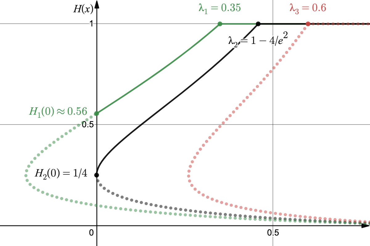
Refer to caption
Figure 13: Diagram of the CDF HμH_{\mu} given by Implicit Equation (3), where a full curve is a well-defined CDF restricted to {(x,Hμ)| 0≤x≤λ​and​(1+1/μ)−2≤Hμ≤1}\{(x,\,H_{\mu})\,|\,0\leq x\leq\lambda~\text{and}~(1+1/\mu)^{-2}\leq H_{\mu}\leq 1\}.
In contrast, a dotted curve is just an analytic continuation, through the same implicit equation, to all Hμ∈[0, 1]H_{\mu}\in[0,\,1]. Such an analytic continuation violates the above restriction and/or Condition (2), so it is not a well-defined CDF supported on [0,λ][0,\,\lambda].
All the three CDF’s in the figure choose the same parameter μ=1\mu=1, so Condition (2) is equivalent to λ≤1−(1+1/μ)2⋅e−2/μ=1−4/e2≈0.4587\lambda\leq 1-(1+1/\mu)^{2}\cdot e^{-2/\mu}=1-4/e^{2}\approx 0.4587. (i) The green full/dotted curves choose a supremum bid λ1=0.35\lambda_{1}=0.35 that lies within the feasible space, by which the yy-axis crosses the implicit equation twice, hence an intersecting line. (ii) The black full/dotted curves choose the boundary-case supremum bid λ2=1−(1+1/μ)2⋅e−2/μ\lambda_{2}=1-(1+1/\mu)^{2}\cdot e^{-2/\mu}, by which the yy-axis just touches the implicit equation, hence a tangent line. (iii) The red dotted curve chooses an infeasible supremum bid λ3=0.6\lambda_{3}=0.6, by which the yy-axis never crosses the implicit equation, hence a disjoint line.
Lemma 5.3 (The ODE; a necessary condition).

Given a supremum bid λ∈(0, 1)\lambda\in(0,\,1), any extremum CDF H∈ℂλ2H\in\mathbb{C}_{\lambda}^{2} of Optimization (IV) satisfies the following ODE for any x∈(0,λ)x\in(0,\,\lambda):

(1−x)⋅(H′​(x))2(H⁡(x)+(1−x)⋅H′​(x))2=2⋅H⁡(x)⋅H′​(x)(H⁡(x)+(1−x)⋅H′​(x))2−2⋅(1−x)⋅(H⁡(x))2⋅H′′​(x)(H⁡(x)+(1−x)⋅H′​(x))3.\displaystyle\frac{(1-x)\cdot(H^{\prime}(x))^{2}}{(H(x)+(1-x)\cdot H^{\prime}(x))^{2}}~=~\frac{2\cdot H(x)\cdot H^{\prime}(x)}{(H(x)+(1-x)\cdot H^{\prime}(x))^{2}}~-~\frac{2\cdot(1-x)\cdot(H(x))^{2}\cdot H^{\prime\prime}(x)}{(H(x)+(1-x)\cdot H^{\prime}(x))^{3}}. (1)
Lemma 5.4 (The ODE solutions).

Given a supremum bid λ∈(0, 1)\lambda\in(0,\,1), any extremum CDF H∈ℂλ2H\in\mathbb{C}_{\lambda}^{2} of Optimization (IV) is determined by one parameter μ>0\mu>0 such that

1−(1+1/μ)2⋅e−2/μ≥λ,\displaystyle 1-(1+1/\mu)^{2}\cdot e^{-2/\mu}~\geq~\lambda, (2)

namely H=HμH=H_{\mu}. Moreover, this extremum CDF HμH_{\mu} is defined by the following implicit equation:

{(x,Hμ)|x=1−(1−λ)⋅Hμ⋅exp⁡((1+1/μ)⋅(2−2​Hμ))such that 0≤x≤λ and (1+1/μ)−2≤Hμ≤1}.\displaystyle\left\{\,(x,\,H_{\mu})\,\,\middle|\,\,\begin{aligned} &x~=~1-(1-\lambda)\cdot H_{\mu}\cdot\exp\Big((1+1/\mu)\cdot\big(2-2\sqrt{H_{\mu}}\big)\Big)\\ &\text{such that $0\leq x\leq\lambda$ and $(1+1/\mu)^{-2}\leq H_{\mu}\leq 1$}\phantom{\bigg.}\end{aligned}\,\right\}. (3)

From subsequent proof details, it will be clear that whenever the parameter μ>0\mu>0 satisfies Condition (2), Implicit Equation (3) does specify a well-defined CDF HμH_{\mu}.

We first establish Lemma 5.3. The proof exploits the Euler-Lagrange equation (stated below as Theorem 12), which is a standard tool from Calculus of Variations.

Theorem 12 (The Euler-Lagrange equation; Calculus of Variations [GS+00]).

Assume the following four premises for the functional 𝒥⁡[f]:=∫x1x2ℒ⁡(x,f⁡(x),f′​(x))⋅𝑑x\mathcal{J}[f]:=\int_{x_{1}}^{x_{2}}\mathcal{L}\big(x,f(x),f^{\prime}(x)\big)\cdot\mathrm{d}x.

  • •

    x1x_{1} and x2x_{2} are constants.

  • •

    f⁡(x)f(x) is twice continuously differentiable.

  • •

    f′​(x)=dd​x​f​(x)f^{\prime}(x)=\frac{\mathrm{d}}{\mathrm{d}x}f(x).

  • •

    ℒ⁡(x,f⁡(x),f′​(x))\mathcal{L}\big(x,f(x),f^{\prime}(x)\big) is twice continuously differentiable with respect to variables xx, ff and f′f^{\prime}.

Then any extremum 𝒥⁡[f]\mathcal{J}[f] satisfies (a necessary condition) the Euler-Lagrange equation

∂ℒ∂f=dd​x​(∂ℒ∂f′)for anyx∈(x1,x2).\displaystyle\frac{\partial\mathcal{L}}{\partial f}~=~\frac{\mathrm{d}}{\mathrm{d}x}\bigg(\frac{\partial\mathcal{L}}{\partial f^{\prime}}\bigg)\quad\text{for any}\quad x\in(x_{1},\,x_{2}).
Remark 13 (The Euler-Lagrange equation).

We emphasize that (i) the LHS of this equation takes the partial derivative of ℒ⁡(x,f,f′)\mathcal{L}(x,f,f^{\prime}) with respect to ff; and (ii) the RHS first regards the partial derivative ∂ℒ∂f′\frac{\partial\mathcal{L}}{\partial f^{\prime}} as a function of one variable xx, and then takes the derivative (with respect to xx).

Now we use the Euler-Lagrange equation to obtain the desired necessary condition. Regarding Optimization (IV), we will consider the following functional.

𝒥⁡[H]:=∫0λℒ⁡(x,H⁡(x),H′​(x))⋅𝑑x,whereℒ⁡(x,H⁡(x),H′​(x)):=H​(x)⋅H′​(x)H⁡(x)+(1−x)⋅H′​(x).\displaystyle\mathcal{J}[H]~:=~\int_{0}^{\lambda}\mathcal{L}\big(x,H(x),H^{\prime}(x)\big)\cdot\mathrm{d}x,\quad\text{where}\quad\mathcal{L}\big(x,H(x),H^{\prime}(x)\big)~:=~\frac{H(x)\cdot H^{\prime}(x)}{H(x)+(1-x)\cdot H^{\prime}(x)}.

Notice that all the four premises of the Euler-Lagrange equation are satisfied:

  • •

    x1=0x_{1}=0 and x2=λx_{2}=\lambda are constants.

  • •

    We only consider those twice continuously differentiable CDF’s H∈ℂλ2H\in\mathbb{C}_{\lambda}^{2}.

  • •

    Obviously H′​(x)=dd​x​H​(x)H^{\prime}(x)=\frac{\mathrm{d}}{\mathrm{d}x}H(x).

  • •

    It is easy to verify that, with respect to variables x∈(0,λ)⊆(0, 1)x\in(0,\,\lambda)\subseteq(0,\,1), H∈[0, 1]H\in[0,\,1] and H′≥0H^{\prime}\geq 0, the integrand ℒ⁡(x,H⁡(x),H′​(x))\mathcal{L}\big(x,H(x),H^{\prime}(x)\big) is twice continuously differentiable.

Proof of Lemma 5.3.

For ease of notation, we would use the shorthands H=H⁡(x)H=H(x), h=H′​(x)h=H^{\prime}(x) and h′=H′′​(x)h^{\prime}=H^{\prime\prime}(x), thus writing the integrand as ℒ⁡(x,H,h)=H⋅hH+(1−x)⋅h\mathcal{L}(x,H,h)=\frac{H\cdot h}{H+(1-x)\cdot h}. Then regarding our functional, the LHS of the Euler-Lagrange equation is given by

∂ℒ∂H=h⋅(H+(1−x)⋅h)−H⋅h(H+(1−x)⋅h)2=(1−x)⋅(H′​(x))2(H⁡(x)+(1−x)⋅H′​(x))2=LHS​ of ODE (1)\frac{\partial\mathcal{L}}{\partial H}~=~\frac{h\cdot(H+(1-x)\cdot h)-H\cdot h}{(H+(1-x)\cdot h)^{2}}~=~\frac{(1-x)\cdot(H^{\prime}(x))^{2}}{(H(x)+(1-x)\cdot H^{\prime}(x))^{2}}~=~{\rm{LHS}}\text{ of ODE~\eqref{eq:ODE}}

where the second step combines the like terms and then substitutes back H=H⁡(x)H=H(x) and h=H′​(x)h=H^{\prime}(x).

Moreover, the partial derivative of ℒ⁡(x,H,h)\mathcal{L}(x,H,h) with respect to variable hh is given by

∂ℒ∂h=H⋅(H+(1−x)⋅h)−(H⋅h)⋅(1−x)(H+(1−x)⋅h)2=H2(H+(1−x)⋅h)2,\frac{\partial\mathcal{L}}{\partial h}~=~\frac{H\cdot(H+(1-x)\cdot h)-(H\cdot h)\cdot(1-x)}{(H+(1-x)\cdot h)^{2}}~=~\frac{H^{2}}{(H+(1-x)\cdot h)^{2}},

where the last step combines the like terms. When being regarded as a function of one variable xx, the derivative of function ∂ℒ∂h\frac{\partial\mathcal{L}}{\partial h} (i.e., the RHS of the Euler-Lagrange equation) is given by

dd​x​(∂ℒ∂h)\displaystyle\frac{\mathrm{d}}{\mathrm{d}x}\bigg(\frac{\partial\mathcal{L}}{\partial h}\bigg) =dd​x​(H2)⋅1(H+(1−x)⋅h)2+H2⋅dd​x​(1(H+(1−x)⋅h)2)\displaystyle~=~\frac{\mathrm{d}}{\mathrm{d}x}\big(H^{2}\big)~\cdot~\frac{1}{(H+(1-x)\cdot h)^{2}}~+~H^{2}~\cdot~\frac{\mathrm{d}}{\mathrm{d}x}\bigg(\frac{1}{(H+(1-x)\cdot h)^{2}}\bigg)
=2⋅H⋅h(H+(1−x)⋅h)2+H2⋅−2⋅(1−x)⋅h′(H+(1−x)⋅h)3\displaystyle~=~\frac{2\cdot H\cdot h}{(H+(1-x)\cdot h)^{2}}\hskip 58.6126pt+~H^{2}\cdot\frac{-2\cdot(1-x)\cdot h^{\prime}}{(H+(1-x)\cdot h)^{3}}\phantom{\bigg.}
=2⋅H⁡(x)⋅H′​(x)(H⁡(x)+(1−x)⋅H′​(x))2−(H(x))2⋅2⋅(1−x)⋅H′′​(x)(H⁡(x)+(1−x)⋅H′​(x))3\displaystyle~=~\frac{2\cdot H(x)\cdot H^{\prime}(x)}{(H(x)+(1-x)\cdot H^{\prime}(x))^{2}}\hskip 22.1931pt-~(H(x))^{2}\cdot\frac{2\cdot(1-x)\cdot H^{\prime\prime}(x)}{(H(x)+(1-x)\cdot H^{\prime}(x))^{3}}\phantom{\bigg.}
=RHS​ of ODE (1),\displaystyle~=~{\rm{RHS}}\text{ of ODE~\eqref{eq:ODE}},\phantom{\bigg.}

where the third step substitutes back H=H⁡(x)H=H(x), h=H′​(x)h=H^{\prime}(x) and h′=H′′​(x)h^{\prime}=H^{\prime\prime}(x).

Therefore, ODE (1) is just a reformulation of the Euler-Lagrange equation and we immediately conclude the lemma from Theorem 12. ∎

In the rest of this subsection, we would resolve ODE (1). For ease of notation, we often write H=H⁡(x)H=H(x), H′=H′​(x)H^{\prime}=H^{\prime}(x) and H′′=H′′​(x)H^{\prime\prime}=H^{\prime\prime}(x). Following Lemma 5.3, we can deduce that

ODE (1)⇔(1−x)⋅(H′)2(H+(1−x)⋅H′)2\displaystyle\text{ODE~\eqref{eq:ODE}}\quad\iff\quad\parbox{95.3169pt}{\hfill$\dfrac{(1-x)\cdot(H^{\prime})^{2}}{(H+(1-x)\cdot H^{\prime})^{2}}$} =2⋅H⋅H′(H+(1−x)⋅H′)2−2⋅(1−x)⋅H2⋅H′′(H+(1−x)⋅H′)3\displaystyle~=~\frac{2\cdot H\cdot H^{\prime}}{(H+(1-x)\cdot H^{\prime})^{2}}~-~\frac{2\cdot(1-x)\cdot H^{2}\cdot H^{\prime\prime}}{(H+(1-x)\cdot H^{\prime})^{3}}\phantom{\bigg.}
⇔2⋅(1−x)⋅H2⋅H′′(H+(1−x)⋅H′)3\displaystyle\iff\quad\parbox{95.3169pt}{\hfill$\dfrac{2\cdot(1-x)\cdot H^{2}\cdot H^{\prime\prime}}{(H+(1-x)\cdot H^{\prime})^{3}}$} =2​H⋅H′(H+(1−x)⋅H′)2−(1−x)⋅(H′)2(H+(1−x)⋅H′)2\displaystyle~=~\frac{2H\cdot H^{\prime}}{(H+(1-x)\cdot H^{\prime})^{2}}~-~\frac{(1-x)\cdot(H^{\prime})^{2}}{(H+(1-x)\cdot H^{\prime})^{2}}\phantom{\bigg.}
⇔2⋅(1−x)⋅H′′H′\displaystyle\iff\quad\parbox{95.3169pt}{\hfill$2\cdot(1-x)\cdot\dfrac{H^{\prime\prime}}{H^{\prime}}$} =(2​H⋅H′−(1−x)⋅(H′)2)⋅H+(1−x)⋅H′H2⋅H′\displaystyle~=~\bigg(2H\cdot H^{\prime}-(1-x)\cdot(H^{\prime})^{2}\bigg)\cdot\frac{H+(1-x)\cdot H^{\prime}}{H^{2}\cdot H^{\prime}}
⇔2⋅(1−x)⋅H′′H′\displaystyle\iff\quad\parbox{95.3169pt}{\hfill$2\cdot(1-x)\cdot\dfrac{H^{\prime\prime}}{H^{\prime}}$} =(2−(1−x)⋅H′H)⋅(1+(1−x)⋅H′H).\displaystyle~=~\bigg(2-(1-x)\cdot\frac{H^{\prime}}{H}\bigg)\cdot\bigg(1+(1-x)\cdot\frac{H^{\prime}}{H}\bigg). (4)

Here the first step restates ODE (1). The second step moves the first term to the RHS and moves the third term to the LHS. The third step first multiplies2929 29 Because x∈(0,λ)x\in(0,\,\lambda) and λ∈(0, 1)\lambda\in(0,\,1), this term ≥1H2⋅H′⋅(32)⋅H2⋅(1−x)⋅H′=3⋅(1−x)\geq\frac{1}{H^{2}\cdot H^{\prime}}\cdot\binom{3}{2}\cdot H^{2}\cdot(1-x)\cdot H^{\prime}=3\cdot(1-x) is strictly positive. the both hand sides by the same term 1H2⋅H′⋅(H+(1−x)⋅H′)3\frac{1}{H^{2}\cdot H^{\prime}}\cdot(H+(1-x)\cdot H^{\prime})^{3} and then simplifies the LHS. And the last step rearranges the RHS.

We define the function z⁡(x):=(1−x)⋅H′​(x)H⁡(x)z(x):=(1-x)\cdot\frac{H^{\prime}(x)}{H(x)} and, for brevity, may write z=z⁡(x)z=z(x) and z′=z′​(x)z^{\prime}=z^{\prime}(x). We have z⁡(x)≥0z(x)\geq 0 for any x∈(0,λ)x\in(0,\,\lambda), since the supremum bid λ∈(0, 1)\lambda\in(0,\,1) and the HH is a nonnegative increasing CDF. Therefore, there exists a nonnegative subset Ω⊆[0,+∞]\Omega\subseteq[0,\,+\infty] such that, over the whole support x∈[0,λ]x\in[0,\,\lambda], the CDF HH can be formulated in term of a parametric equation

{(x,H)=(𝒳⁡(z),ℋ⁡(z))|z∈Ω}.\Big\{\,(x,\,H)=\big(\mathcal{X}(z),\,\mathcal{H}(z)\big)\,\,\Big|\,\Big.\,z\in\Omega\,\Big\}.

Below we would capture the analytic formulas x=𝒳⁡(z)x=\mathcal{X}(z) and H=ℋ⁡(z)H=\mathcal{H}(z) and then (in the proof of Lemma 5.4) study the condition for which the above parametric equation does yield a CDF HH that is well defined on the support x∈[0,λ]x\in[0,\,\lambda].

Proof of the x=𝒳⁡(z)x=\mathcal{X}(z) formula.

We can deduce that

z⋅H\displaystyle z\cdot H =(1−x)⋅H′\displaystyle~=~(1-x)\cdot H^{\prime} ⟸\displaystyle\Longleftarrow definition of z⁡(x)z(x)    
z′⋅H+z⋅H′\displaystyle z^{\prime}\cdot H~+~z\cdot H^{\prime} =−H′+(1−x)⋅H′′\displaystyle~=~-H^{\prime}~+~(1-x)\cdot H^{\prime\prime} ⟸\displaystyle\Longleftarrow take derivative    
(1−x)⋅H′′H′\displaystyle(1-x)\cdot\frac{H^{\prime\prime}}{H^{\prime}} =1+z+z′⋅HH′\displaystyle~=~1~+~z~+~z^{\prime}\cdot\frac{H}{H^{\prime}} ⟸\displaystyle\Longleftarrow multiply 1/H′1\big/H^{\prime} and rearrange    
(1−x)⋅H′′H′\displaystyle(1-x)\cdot\frac{H^{\prime\prime}}{H^{\prime}} =1+z+(1−x)⋅z′z\displaystyle~=~1~+~z~+~(1-x)\cdot\frac{z^{\prime}}{z} ⟸\displaystyle\Longleftarrow substitute H/H′=1−xzH\big/H^{\prime}=\frac{1-x}{z} for the RHS    

Apply this identity (resp. the definition z=(1−x)⋅H′Hz=(1-x)\cdot\frac{H^{\prime}}{H}) to the LHS (resp. RHS) of ODE (4):

ODE (4)⇔2⋅(1+z+(1−x)⋅z′z)\displaystyle\text{ODE~\eqref{eq:solve_ODE:1}}\quad\iff\quad\parbox{123.76965pt}{\hfill$2\cdot\bigg(1+z+(1-x)\cdot\dfrac{z^{\prime}}{z}\bigg)$} =(2−z)⋅(1+z)\displaystyle~=~(2-z)\cdot(1+z)
⇔2⋅(1−x)⋅z′z\displaystyle\iff\quad\parbox{123.76965pt}{\hfill$2\cdot(1-x)\cdot\dfrac{z^{\prime}}{z}$} =−z⋅(1+z)\displaystyle~=~-z\cdot(1+z)\phantom{\bigg.}
⇔2z2⋅(1+z)⋅z′\displaystyle\iff\quad\parbox{123.76965pt}{\hfill$\dfrac{2}{z^{2}\cdot(1+z)}\cdot z^{\prime}$} =−11−x.\displaystyle~=~\frac{-1}{1-x}. (5)

Here the second step cancels the common term (2+2​z)(2+2z) on the both hand sides. And the last step multiplies the both hand sides by the same positive term 1(1−x)⋅z⋅(1+z)\frac{1}{(1-x)\cdot z\cdot(1+z)}.

We denote μ=z⁡(λ)\mu=z(\lambda) for some parameter μ>0\mu>0, namely the boundary condition for (5) as a partial differential equation (PDE). For this PDE, the integration of the LHS on any interval between z=z⁡(x)z=z(x) and μ=z⁡(λ)\mu=z(\lambda), is equal to that of the RHS on the corresponding interval between xx and λ\lambda. Namely, we have

PDE (5)⟹∫μz2y2⋅(1+y)⋅dy\displaystyle\text{PDE~\eqref{eq:solve_ODE:2}}\quad\Longrightarrow\quad\parbox{135.15059pt}{\hfill$\displaystyle{\int_{\mu}^{z}\frac{2}{y^{2}\cdot(1+y)}\cdot\mathrm{d}y}$} =∫λx−11−y⋅𝑑y\displaystyle~=~\int_{\lambda}^{x}\frac{-1}{1-y}\cdot\mathrm{d}y
⟹(2​ln⁡(1+1/y)−2/y)|y=μz\displaystyle\Longrightarrow\quad\parbox{135.15059pt}{\hfill$\Big(2\ln(1+1/y)-2/y\Big)\,\Big|\,\Big._{y\,=\,\mu}^{z}$} =ln⁡(1−y)|y=λx\displaystyle~=~\ln(1-y)\,\Big|\,\Big._{y\,=\,\lambda}^{x}\phantom{\bigg.}
⟹2​ln⁡(1+1/z1+1/μ)−2/z+2/μ\displaystyle\Longrightarrow\quad\parbox{135.15059pt}{\hfill$\displaystyle{2\ln\bigg(\frac{1+1/z}{1+1/\mu}\bigg)-2/z+2/\mu}$} =ln⁡(1−x)−ln⁡(1−λ)\displaystyle~=~\ln(1-x)-\ln(1-\lambda)
⟹\displaystyle\Longrightarrow\quad\parbox{135.15059pt}{\phantom{}} x=𝒳(z)=1−1−λ(1+1/μ)2⋅e−2/μ⋅(1+1/z)2⋅e−2/z,\displaystyle\hskip-135.15059ptx~=~\mathcal{X}(z)~=~1-\frac{1-\lambda}{(1+1/\mu)^{2}\cdot e^{-2/\mu}}\cdot(1+1/z)^{2}\cdot e^{-2/z},\phantom{\bigg.} (6)

where the last step rearranges the equation. Notably, at z=μz=\mu we achieve the supremum bid 𝒳⁡(μ)=λ\mathcal{X}(\mu)=\lambda.

Formula (6) is precisely the first part x=𝒳⁡(z)x=\mathcal{X}(z) of our parametric equation. ∎

Proof of the H=ℋ⁡(z)H=\mathcal{H}(z) formula.

To further obtain this formula, we observe that

1H⋅d​Hd​x=H′H=z1−x=(1+1/μ)2⋅e−2/μ1−λ⋅z(1+1/z)2⋅e−2/z,\displaystyle\frac{1}{H}\cdot\frac{\mathrm{d}H}{\mathrm{d}x}~=~\frac{H^{\prime}}{H}~=~\frac{z}{1-x}~=~\frac{(1+1/\mu)^{2}\cdot e^{-2/\mu}}{1-\lambda}\cdot\frac{z}{(1+1/z)^{2}\cdot e^{-2/z}}, (7)

where the second step applies the definition z=(1−x)⋅H′Hz=(1-x)\cdot\frac{H^{\prime}}{H} and the last step applies Formula (6). Moreover, the derivative of function 𝒳⁡(z)\mathcal{X}(z) is given by

𝒳′​(z)=d​xd​z\displaystyle\mathcal{X}^{\prime}(z)~=~\frac{\mathrm{d}x}{\mathrm{d}z} =−1−λ(1+1/μ)2⋅e−2/μ⋅dd​z((1+1/z)2⋅e−2/z)\displaystyle~=~-\frac{1-\lambda}{(1+1/\mu)^{2}\cdot e^{-2/\mu}}\cdot\frac{\mathrm{d}}{\mathrm{d}z}\bigg((1+1/z)^{2}\cdot e^{-2/z}\bigg)
=−1−λ(1+1/μ)2⋅e−2/μ⋅(2⋅(1+1/z)⋅−1z2⋅e−2/z+(1+1/z)2⋅e−2/z⋅2z2)\displaystyle~=~-\frac{1-\lambda}{(1+1/\mu)^{2}\cdot e^{-2/\mu}}\cdot\bigg(2\cdot(1+1/z)\cdot\frac{-1}{z^{2}}\cdot e^{-2/z}+(1+1/z)^{2}\cdot e^{-2/z}\cdot\frac{2}{z^{2}}\bigg)
=−1−λ(1+1/μ)2⋅e−2/μ⋅2⋅(1+1/z)⋅e−2/zz3,\displaystyle~=~-\frac{1-\lambda}{(1+1/\mu)^{2}\cdot e^{-2/\mu}}\cdot\frac{2\cdot(1+1/z)\cdot e^{-2/z}}{z^{3}}, (8)

where the first step applies Formula (6) and the last step combines the like terms. Notice that this derivative 𝒳′​(z)\mathcal{X}^{\prime}(z) is strictly negative, so 𝒳⁡(z)\mathcal{X}(z) is a strictly decreasing function.

Combining Equations 7 and 8 together gives

(ln⁡ℋ⁡(z))′\displaystyle\big(\ln\mathcal{H}(z)\big)^{\prime} =dd​z​(ln⁡H)=1H⋅d​Hd​z=(1H⋅d​Hd​x)⋅(d​xd​z)\displaystyle~=~\frac{\mathrm{d}}{\mathrm{d}z}\big(\ln H\big)~=~\frac{1}{H}\cdot\frac{\mathrm{d}H}{\mathrm{d}z}~=~\bigg(\frac{1}{H}\cdot\frac{\mathrm{d}H}{\mathrm{d}x}\bigg)\cdot\bigg(\frac{\mathrm{d}x}{\mathrm{d}z}\bigg)
=(z(1+1/z)2⋅e−2/z)⋅(−2⋅(1+1/z)⋅e−2/zz3)\displaystyle~=~\bigg(\frac{z}{(1+1/z)^{2}\cdot e^{-2/z}}\bigg)\cdot\bigg(-\frac{2\cdot(1+1/z)\cdot e^{-2/z}}{z^{3}}\bigg)
=−2z⋅(z+1).\displaystyle~=~\frac{-2}{z\cdot(z+1)}. (9)

This ODE (9) must admit the boundary condition ℋ⁡(μ)=1\mathcal{H}(\mu)=1, given that (as mentioned) at z=μz=\mu we achieve the supremum bid 𝒳⁡(μ)=λ\mathcal{X}(\mu)=\lambda. For this reason, taking the integration of the both hand sides on any interval [μ,z][\mu,\,z] gives

ODE (9)⟹∫μz(ln⁡ℋ⁡(y))′⋅dy\displaystyle\text{ODE~\eqref{eq:solve_ODE:6}}\quad\Longrightarrow\quad\parbox{86.78099pt}{\hfill$\displaystyle{\int_{\mu}^{z}\big(\ln\mathcal{H}(y)\big)^{\prime}\cdot\mathrm{d}y}$} =∫μz−2y⋅(y+1)⋅𝑑y\displaystyle~=~\int_{\mu}^{z}\frac{-2}{y\cdot(y+1)}\cdot\mathrm{d}y
⟹ln⁡ℋ⁡(z)−ln⁡ℋ⁡(μ)\displaystyle\Longrightarrow\quad\parbox{86.78099pt}{\hfill$\ln\mathcal{H}(z)-\ln\mathcal{H}(\mu)$} =(2​ln⁡(1+1/y))|y=μz\displaystyle~=~\Big(2\ln(1+1/y)\Big)\,\Big|\,\Big._{y\,=\,\mu}^{z}\phantom{\bigg.}
⟹ln⁡ℋ⁡(z)\displaystyle\Longrightarrow\quad\parbox{86.78099pt}{\hfill$\ln\mathcal{H}(z)$} =2​ln⁡(1+1/z1+1/μ)\displaystyle~=~2\ln\bigg(\frac{1+1/z}{1+1/\mu}\bigg)
⟹H=ℋ⁡(z)\displaystyle\Longrightarrow\quad\parbox{86.78099pt}{\hfill$H~=~\mathcal{H}(z)$} =(1+1/z)2(1+1/μ)2.\displaystyle~=~\frac{(1+1/z)^{2}}{(1+1/\mu)^{2}}. (10)

where the third step applies the boundary condition ℋ⁡(μ)=1\mathcal{H}(\mu)=1 to the LHS. Notice that ℋ⁡(z)\mathcal{H}(z) is a strictly decreasing function.

Formula (10) is precisely the second part H=ℋ⁡(z)H=\mathcal{H}(z) of our parametric equation. ∎

Based on the above discussions, we are able to prove Lemma 5.4.

Proof of Lemma 5.4.

We first check Condition (2) and then capture Implicit Equation (3).

Condition (2). As mentioned, both of 𝒳⁡(z)\mathcal{X}(z) and ℋ⁡(z)\mathcal{H}(z) are strictly decreasing functions (Equations 8 and 10). Moreover, at z=μz=\mu we achieve the supremum bid 𝒳⁡(μ)=λ\mathcal{X}(\mu)=\lambda and the boundary condition ℋ⁡(μ)=1\mathcal{H}(\mu)=1. By considering all possible parameters z∈[μ,+∞]z\in[\mu,\,+\infty], our parametric equation (𝒳⁡(z),ℋ⁡(z))\big(\mathcal{X}(z),\,\mathcal{H}(z)\big) yields a strictly increasing function H¯\overline{H} with the domain x∈[𝒳⁡(+∞),λ]x\in[\mathcal{X}(+\infty),\,\lambda]. In this domain, function H¯\overline{H} is bounded between ℋ⁡(+∞)=(1+1/μ)−2≥0\mathcal{H}(+\infty)=(1+1/\mu)^{-2}\geq 0 and ℋ⁡(μ)=1\mathcal{H}(\mu)=1.

This function H¯\overline{H} must be consistent with the considered CDF HH. In this way, we require that: (i) the support x∈[0,λ]x\in[0,\,\lambda] of CDF HH is a subset of the domain x∈[𝒳⁡(+∞),λ]x\in[\mathcal{X}(+\infty),\,\lambda] of function H¯\overline{H}; and, if so, (ii) function H¯\overline{H} can be a well-defined CDF on the support x∈[0,λ]x\in[0,\,\lambda].

Clearly, the first requirement is equivalent to

0≥𝒳⁡(+∞)=1−(1−λ)⋅(1+1/μ)−2⋅e2/μ,0~\geq~\mathcal{X}(+\infty)~=~1-(1-\lambda)\cdot(1+1/\mu)^{-2}\cdot e^{2/\mu},

which after being rearranged gives Condition (2). Indeed, the first requirement ensures the second one – function H¯\overline{H} is strictly increasing and is bounded between ℋ⁡(+∞)=(1+1/μ)−2≥0\mathcal{H}(+\infty)=(1+1/\mu)^{-2}\geq 0 and ℋ⁡(μ)=1\mathcal{H}(\mu)=1 in the whole domain x∈[𝒳⁡(+∞),λ]x\in[\mathcal{X}(+\infty),\,\lambda], thus (once the first requirement is satisfied) being a well-defined CDF on the support x∈[0,λ]⊆[𝒳⁡(+∞),λ]x\in[0,\,\lambda]\subseteq[\mathcal{X}(+\infty),\,\lambda].

Implicit Equation (3). We reformulate our parametric equation (x,H)=(𝒳⁡(z),ℋ⁡(z))(x,\,H)=\big(\mathcal{X}(z),\,\mathcal{H}(z)\big) below, which precisely gives the claimed implicit equation.

Formula (6)⇔x\displaystyle\text{Formula~\eqref{eq:solve_ODE:3}}~~\iff~~x =1−1−λ(1+1/μ)2⋅e−2/μ⋅(1+1/z)2⋅e−2/z\displaystyle~=~1-\frac{1-\lambda}{(1+1/\mu)^{2}\cdot e^{-2/\mu}}\cdot(1+1/z)^{2}\cdot e^{-2/z}\phantom{\bigg.}
=1−1−λ(1+1/μ)2⋅e−2/μ⋅((1+1/μ)2⋅H)⋅exp⁡(2−(1+1/μ)⋅2​H)\displaystyle~=~1-\frac{1-\lambda}{(1+1/\mu)^{2}\cdot e^{-2/\mu}}\cdot\Big((1+1/\mu)^{2}\cdot H\Big)\cdot\exp\Big(2-(1+1/\mu)\cdot 2\sqrt{H}\Big)\phantom{\bigg.}
=1−(1−λ)⋅H⋅exp⁡((1+1/μ)⋅(2−2​H)).\displaystyle~=~1-(1-\lambda)\cdot H\cdot\exp\Big((1+1/\mu)\cdot\big(2-2\sqrt{H}\big)\Big).\phantom{\bigg.}

Here the first step restates Formula (6). The second step (Formula (10)) substitutes (1+1/z)2=(1+1/μ)2⋅H(1+1/z)^{2}=(1+1/\mu)^{2}\cdot H and −1/z=1−(1+1/μ)⋅H-1/z=1-(1+1/\mu)\cdot\sqrt{H}.3030 30 Since the variable z∈[μ,+∞]z\in[\mu,\,+\infty] is positive, we safely ignore the other (impossible) case −1/z=1+(1+1/μ)⋅H-1/z=1+(1+1/\mu)\cdot\sqrt{H}. And the last step rearranges the equation.

Combining Condition (2) and Implicit Equation (3) together finishes the proof. ∎

As an implication of Lemma 5.4, by setting x=0x=0 in Implicit Equation (3) we can characterize the pointmass hμ:=Hμ​(0)h_{\mu}:=H_{\mu}(0) of a candidate worst-case CDF. This is formalized into Corollary 5.5. Also, because Lemma 5.4 holds for any given supremum bid λ∈(0, 1)\lambda\in(0,\,1), combining it with Lemma 5.2 gives Corollary 5.6. These two corollaries are more convenient for our later use.

Corollary 5.5 (The ODE solutions).

Given a supremum bid λ∈(0, 1)\lambda\in(0,\,1) and a parameter μ>0\mu>0 that meets Condition (2), the CDF HμH_{\mu} defined by Implicit Equation (3) has a pointmass hμ:=Hμ​(0)h_{\mu}:=H_{\mu}(0) at x=0x=0, which is the unique solution to the following equation:

{1=(1−λ)⋅hμ⋅exp⁡((1+1/μ)⋅(2−2​hμ))such that (1+1/μ)−2≤hμ<1}.\displaystyle\left\{\,~\begin{aligned} &1~=~(1-\lambda)\cdot h_{\mu}\cdot\exp\Big((1+1/\mu)\cdot\big(2-2\sqrt{h_{\mu}}\big)\Big)\\ &\text{such that $(1+1/\mu)^{-2}\leq h_{\mu}<1$}\phantom{\bigg.}\end{aligned}~\,\right\}.
Corollary 5.6 (Price of Anarchy).

Regarding First Price Auctions, the Price of Anarchy satisfies that

𝖯𝗈𝖠≥1−sup{(1−λ)⋅∫0λHμ​(x)⋅Hμ′​(x)⋅d​xHμ​(x)+(1−x)⋅Hμ′​(x)|0<μ<+∞0<λ≤1−(1+1/μ)2⋅e−2/μ}.\displaystyle{\sf PoA}~\geq~1-\sup\left\{\,(1-\lambda)\cdot\int_{0}^{\lambda}\frac{H_{\mu}(x)\cdot H^{\prime}_{\mu}(x)\cdot\mathrm{d}x}{H_{\mu}(x)+(1-x)\cdot H^{\prime}_{\mu}(x)}\,\,\middle|\,\,\begin{aligned} &0<\mu<+\infty\\ &0<\lambda\leq 1-(1+1/\mu)^{2}\cdot e^{-2/\mu}\end{aligned}\,\right\}.
Proof.

Applying Lemma 5.4 to Optimization (III) gives an interim optimization that takes the supremum operation twice: (i) the inner operation, according to Condition (2), works on feasible space {μ>0| 1−(1+1/μ)2⋅e−2/μ≥λ}\big\{\,\mu>0\,\,\big|\,\big.\,1-(1+1/\mu)^{2}\cdot e^{-2/\mu}\geq\lambda\,\big\} given by the λ∈(0, 1)\lambda\in(0,\,1); and (ii) the outer operation works on feasible space λ∈(0, 1)\lambda\in(0,\,1). Switching the order of both operations gives the corollary. ∎

5.3 Optimizing the parameters (λ,μ)(\lambda,\,\mu)

We solve the optimization in Corollary 5.6 in two steps: (i) Lemma 5.7 transforms the considered integral formula into an equivalent analytic formula, Optimization (V); and (ii) Lemma 5.8 further derives the analytic solution, i.e., finding the (unique) worst case (λ∗,μ∗)(\lambda^{*},\,\mu^{*}) of Optimization (V).

Lemma 5.7 (Price of Anarchy).

Regarding First Price Auctions, the Price of Anarchy satisfies that

𝖯𝗈𝖠≥1−sup{(1−λ)⋅((1−hμ)−2−2​hμ1+1/μ)|0<μ<+∞0<λ≤1−(1+1/μ)2⋅e−2/μhμ defined by Corollary 5.5}.\displaystyle{\sf PoA}~\geq~1-\sup\left\{\,(1-\lambda)\cdot\bigg((1-h_{\mu})-\frac{2-2\sqrt{h_{\mu}}}{1+1/\mu}\bigg)\,\,\middle|\,\,\begin{aligned} &0<\mu<+\infty\\ &0<\lambda\leq 1-(1+1/\mu)^{2}\cdot e^{-2/\mu}\\ &\text{$h_{\mu}$ defined by \lx@cref{creftypecap\lx@tilde refnum}{cor:pointmass}}\end{aligned}\,\right\}. (V)
Lemma 5.8 (Worst case).

The solution to Optimization (V) is 1−1/e2≈0.86471-1/e^{2}\approx 0.8647, which can be achieved by the worst case (λ∗,μ∗)=(1−4/e2, 1)(\lambda^{*},\,\mu^{*})=(1-4/e^{2},\,1) and the resulting pointmass hμ∗=1/4h_{\mu^{*}}=1/4.

Proof of Lemma 5.7.

Following Corollary 5.6, given any feasible pair (λ,μ)(\lambda,\,\mu), we study the integral

(1−λ)⋅∫0λHμ​(x)⋅Hμ′​(x)⋅d​xHμ​(x)+(1−x)⋅Hμ′​(x)\displaystyle(1-\lambda)\cdot\int_{0}^{\lambda}\frac{H_{\mu}(x)\cdot H^{\prime}_{\mu}(x)\cdot\mathrm{d}x}{H_{\mu}(x)+(1-x)\cdot H^{\prime}_{\mu}(x)} =(1−λ)⋅∫x∈[0,λ]Hμ⋅(d​Hμ/d​x)⋅d​xHμ+(1−x)⋅(d​Hμ/d​x)\displaystyle~=~(1-\lambda)\cdot\int_{x\,\in\,[0,\,\lambda]}\frac{H_{\mu}\cdot\big(\mathrm{d}H_{\mu}\big/\mathrm{d}x\big)\cdot\mathrm{d}x}{H_{\mu}+(1-x)\cdot\big(\mathrm{d}H_{\mu}\big/\mathrm{d}x\big)}
=(1−λ)⋅∫Hμ∈[hμ, 1]Hμ⋅d​HμHμ+(1−x)/(d​x/d​Hμ),\displaystyle~=~(1-\lambda)\cdot\int_{H_{\mu}\,\in\,[h_{\mu},\,1]}\frac{H_{\mu}\cdot\mathrm{d}H_{\mu}}{H_{\mu}+(1-x)\big/(\mathrm{d}x/\mathrm{d}H_{\mu})}, (11)

where the last step changes the variables. We aim to give an analytic formula for the term 1−xd​x/d​Hμ\frac{1-x}{\mathrm{d}x/\mathrm{d}H_{\mu}}. To this end, let us regard Implicit Equation (3) as a function x⁡(Hμ)x(H_{\mu}) of variable Hμ∈[hμ, 1]H_{\mu}\in[h_{\mu},\,1] (i.e., the inverse function of the considered CDF), then the derivative is given by

d​xd​Hμ\displaystyle\frac{\mathrm{d}x}{\mathrm{d}H_{\mu}} =−(1−λ)⋅dd​Hμ(Hμ⋅exp((1+1/μ)⋅(2−2Hμ)))\displaystyle~=~-(1-\lambda)\cdot\frac{\mathrm{d}}{\mathrm{d}H_{\mu}}\bigg(H_{\mu}\cdot\exp\Big((1+1/\mu)\cdot\big(2-2\sqrt{H_{\mu}}\big)\Big)\bigg)
=−(1−λ)⋅(exp((1+1/μ)⋅(2−2Hμ))\displaystyle~=~-(1-\lambda)\cdot\bigg(\exp\Big((1+1/\mu)\cdot\big(2-2\sqrt{H_{\mu}}\big)\Big)\Bigg.
+Hμ⋅exp((1+1/μ)⋅(2−2Hμ))⋅(1+1/μ)⋅−1Hμ)\displaystyle\phantom{~=~}\hskip 71.13188pt~+~\bigg.H_{\mu}\cdot\exp\Big((1+1/\mu)\cdot\big(2-2\sqrt{H_{\mu}}\big)\Big)\cdot(1+1/\mu)\cdot\frac{-1}{\sqrt{H_{\mu}}}\bigg)
=−(1−λ)⋅(1−(1+1/μ)⋅Hμ)⋅exp((1+1/μ)⋅(2−2Hμ))\displaystyle~=~-(1-\lambda)\cdot\Big(1-(1+1/\mu)\cdot\sqrt{H_{\mu}}\Big)\cdot\exp\Big((1+1/\mu)\cdot\big(2-2\sqrt{H_{\mu}}\big)\Big)\phantom{\bigg.}

Combining this formula with Implicit Equation (3) gives

1−xd​x/d​Hμ\displaystyle\frac{1-x}{\mathrm{d}x\big/\mathrm{d}H_{\mu}} =(1−λ)⋅Hμ⋅exp⁡((1+1/μ)⋅(2−2​Hμ))−(1−λ)⋅(1−(1+1/μ)⋅Hμ)⋅exp((1+1/μ)⋅(2−2Hμ))\displaystyle~=~\frac{\phantom{-}(1-\lambda)\cdot\parbox{110.39682pt}{\centering$H_{\mu}$\@add@centering}\cdot\exp\Big((1+1/\mu)\cdot\big(2-2\sqrt{H_{\mu}}\big)\Big)}{-(1-\lambda)\cdot\Big(1-(1+1/\mu)\cdot\sqrt{H_{\mu}}\Big)\cdot\exp\Big((1+1/\mu)\cdot\big(2-2\sqrt{H_{\mu}}\big)\Big)}
=Hμ(1+1/μ)⋅Hμ−1.\displaystyle~=~\frac{H_{\mu}}{(1+1/\mu)\cdot\sqrt{H_{\mu}}-1}.

Plugging this analytic formula for the term 1−xd​x/d​Hμ\frac{1-x}{\mathrm{d}x/\mathrm{d}H_{\mu}} back to Integral (11) gives

Integral (11) =(1−λ)⋅∫Hμ∈[hμ, 1]Hμ⋅d​HμHμ+Hμ(1+1/μ)⋅Hμ−1\displaystyle~=~(1-\lambda)\cdot\int_{H_{\mu}\,\in\,[h_{\mu},\,1]}\frac{H_{\mu}\cdot\mathrm{d}H_{\mu}}{H_{\mu}+\frac{H_{\mu}}{(1+1/\mu)\cdot\sqrt{H_{\mu}}-1}}
=(1−λ)⋅∫Hμ∈[hμ, 1](1−1(1+1/μ)⋅Hμ)⋅d​Hμ\displaystyle~=~(1-\lambda)\cdot\int_{H_{\mu}\in[h_{\mu},\,1]}\bigg(1-\frac{1}{(1+1/\mu)\cdot\sqrt{H_{\mu}}}\bigg)\cdot\mathrm{d}H_{\mu}
=(1−λ)⋅(Hμ−2​Hμ1+1/μ)|Hμ=hμ1\displaystyle~=~(1-\lambda)\cdot\bigg(H_{\mu}-\frac{2\sqrt{H_{\mu}}}{1+1/\mu}\bigg)\,\bigg|\,\bigg._{H_{\mu}\,=\,h_{\mu}}^{1}
=(1−λ)⋅((1−hμ)−2−2​hμ1+1/μ),\displaystyle~=~(1-\lambda)\cdot\bigg((1-h_{\mu})-\frac{2-2\sqrt{h_{\mu}}}{1+1/\mu}\bigg),

which is precisely the formula in Optimization (V). This finishes the proof of the lemma. ∎

Optimization (V) involves just three variables and, indeed, one of them hμh_{\mu} is even determined by the other two (λ,μ)(\lambda,\,\mu). Lemma 5.8 gives the analytic solution to Optimization (V).

Proof of Lemma 5.8.

For the moment, we regard the μ>0\mu>0 as a given parameter. It follows from Corollary 5.5 that λ=G⁡(hμ)\lambda=G(h_{\mu}), where the function GG is defined in the domain hμ∈[(1+1/μ)−2, 1)h_{\mu}\in\big[(1+1/\mu)^{-2},\,1\big):

G(hμ):=1−(1/hμ)⋅exp(−(2−2hμ)⋅(1+1/μ)).\displaystyle G(h_{\mu})~:=~1-(1/h_{\mu})\cdot\exp\Big(-\big(2-2\sqrt{h_{\mu}}\big)\cdot(1+1/\mu)\Big).

This G⁡(hμ)G(h_{\mu}) is a continuous function. And for any hμ>(1+1/μ)−2h_{\mu}>(1+1/\mu)^{-2}, its derivative

G′​(hμ)\displaystyle G^{\prime}(h_{\mu}) =(1/hμ2)⋅exp(−(2−2hμ)⋅(1+1/μ))\displaystyle~=~(1/h_{\mu}^{2})\cdot\exp\Big(-\big(2-2\sqrt{h_{\mu}}\big)\cdot(1+1/\mu)\Big)
−(1/hμ)⋅exp(−(2−2hμ)⋅(1+1/μ))⋅((1+1/μ)/hμ)\displaystyle\hskip 28.45274pt~-~(1/h_{\mu})\cdot\exp\Big(-\big(2-2\sqrt{h_{\mu}}\big)\cdot(1+1/\mu)\Big)\cdot\Big((1+1/\mu)\big/\sqrt{h_{\mu}}\Big)
=(1/hμ2)⋅exp(−(2−2hμ)⋅(1+1/μ))⋅(1−(1+1/μ)⋅hμ)\displaystyle~=~(1/h_{\mu}^{2})\cdot\exp\Big(-\big(2-2\sqrt{h_{\mu}}\big)\cdot(1+1/\mu)\Big)\cdot\Big(1-(1+1/\mu)\cdot\sqrt{h_{\mu}}\Big)

is strictly positive. Thus, this function G⁡(hμ)G(h_{\mu}) is strictly increasing in the whole left-closed right-open domain hμ∈[(1+1/μ)−2, 1)h_{\mu}\in\big[(1+1/\mu)^{-2},\,1\big). Moreover, the image of function G⁡(hμ)G(h_{\mu}),

{G(hμ)|(1+1/μ)−2≤hμ<1}=(0, 1−(1+1/μ)2⋅e−2/μ]\Big\{\,G(h_{\mu})\,\,\Big|\,\Big.\,(1+1/\mu)^{-2}\leq h_{\mu}<1\,\Big\}~=~\big(0,\,1-(1+1/\mu)^{2}\cdot e^{-2/\mu}\big]

is precisely the feasible space of λ\lambda in Optimization (V), which means the mapping between all feasible λ\lambda and all hμ∈[(1+1/μ)−2, 1)h_{\mu}\in\big[(1+1/\mu)^{-2},\,1\big) is one-to-one. For these reasons, we can deduce that

Optimization (V) =1−sup{(1−G⁡(hμ))⋅((1−hμ)−2−2​hμ1+1/μ)|0<μ<+∞(1+1/μ)−2≤hμ<1}\displaystyle~=~1-\sup\left\{\,\big(1-G(h_{\mu})\big)\cdot\bigg((1-h_{\mu})-\frac{2-2\sqrt{h_{\mu}}}{1+1/\mu}\bigg)\phantom{\frac{}{\Big.}}\,\middle|\,\,\begin{aligned} &0<\mu<+\infty\\ &(1+1/\mu)^{-2}\leq h_{\mu}<1\end{aligned}\,\right\}
=1−sup{(1−hμ)−(2−2​hμ)⋅(1+1/μ)−1hμ⋅exp⁡((2−2​hμ)⋅(1+1/μ))|0<μ<+∞(1+1/μ)−2≤hμ<1}\displaystyle~=~1-\sup\left\{\,\frac{(1-h_{\mu})-\big(2-2\sqrt{h_{\mu}}\big)\cdot(1+1/\mu)^{-1}}{h_{\mu}\cdot\exp\Big(\big(2-2\sqrt{h_{\mu}}\big)\cdot(1+1/\mu)\Big)}\,\,\middle|\,\,\begin{aligned} &0<\mu<+\infty\\ &(1+1/\mu)^{-2}\leq h_{\mu}<1\end{aligned}\,\right\}
=1−sup{𝒢⁡(β,γ):=(1−β2)−(2−2​β)⋅γβ2⋅exp⁡((2−2​β)⋅γ−1)|0<γ≤β<1},\displaystyle~=~1-\sup\left\{\,\mathcal{G}(\beta,\,\gamma):=\frac{(1-\beta^{2})-(2-2\beta)\cdot\gamma}{\beta^{2}\cdot\exp\big((2-2\beta)\cdot\gamma^{-1}\big)}\phantom{\frac{}{\Big.}}\,\middle|\,\,\text{$0<\gamma\leq\beta<1$}\,\right\},

where the first step switches the optimization variable from λ\lambda to hμ∈[(1+1/μ)−2, 1)h_{\mu}\in\big[(1+1/\mu)^{-2},\,1\big), the second step plugs the G⁡(hμ)G(h_{\mu}) formula, and the last step substitutes β:=hμ\beta:=\sqrt{h_{\mu}} and γ:=(1+1/μ)−1\gamma:=(1+1/\mu)^{-1}.

Below we would reason about the function 𝒢⁡(β,γ)\mathcal{G}(\beta,\,\gamma) defined above. The partial derivative of this function with respect to variable γ\gamma is given by

∂𝒢∂γ\displaystyle\frac{\partial\mathcal{G}}{\partial\gamma} =−(2−2​β)β2⋅exp⁡((2−2​β)⋅γ−1)+(1−β2)−(2−2​β)⋅γβ2⋅exp⁡((2−2​β)⋅γ−1)⋅(2−2​β)⋅γ−2\displaystyle~=~\frac{-(2-2\beta)}{\beta^{2}\cdot\exp\big((2-2\beta)\cdot\gamma^{-1}\big)}~+~\frac{(1-\beta^{2})-(2-2\beta)\cdot\gamma}{\beta^{2}\cdot\exp\big((2-2\beta)\cdot\gamma^{-1}\big)}\cdot(2-2\beta)\cdot\gamma^{-2}
=(1−β2)−(2−2​β)⋅γ−γ2β2⋅exp⁡((2−2​β)⋅γ−1)⋅(2−2​β)⋅γ−2,\displaystyle~=~\frac{(1-\beta^{2})-(2-2\beta)\cdot\gamma-\gamma^{2}}{\beta^{2}\cdot\exp\big((2-2\beta)\cdot\gamma^{-1}\big)}\cdot(2-2\beta)\cdot\gamma^{-2},

where the last step rearranges the formula. Clearly, in the feasible space {0<γ≤β<1}\{0<\gamma\leq\beta<1\}, the sign of this partial derivative ∂𝒢/∂γ\partial\mathcal{G}\big/\partial\gamma depends on the numerator (1−β2)−2​γ⋅(1−β)−γ2(1-\beta^{2})-2\gamma\cdot(1-\beta)-\gamma^{2}.

Refer to caption
Figure 14: Diagram of (the red curve) the 𝒢⁡(β,β)\mathcal{G}(\beta,\,\beta) as an increasing function of β∈(0, 1/2]\beta\in(0,\,1/2] and (the blue curve) the 𝒢⁡(β,γβ)\mathcal{G}(\beta,\,\gamma_{\beta}) as a decreasing function of β∈(1/2, 1)\beta\in(1/2,\,1).

For the moment, we regard β∈(0, 1)\beta\in(0,\,1) as a given parameter and consider the parabola

Pβ​(γ):=(1−β2)−2​γ⋅(1−β)−γ2P_{\beta}(\gamma)~:=~(1-\beta^{2})-2\gamma\cdot(1-\beta)-\gamma^{2}

in the domain γ∈[0,β]\gamma\in[0,\,\beta]. This parabola opens downwards and has a nonpositive axis of symmetry γ=−(1−β)\gamma=-(1-\beta), thus being a decreasing function in the whole domain γ∈[0,β]\gamma\in[0,\,\beta]. Also, the left/right ends are respectively Pβ​(0)=1−β2>0P_{\beta}(0)=1-\beta^{2}>0 and Pβ​(β)=1−2​βP_{\beta}(\beta)=1-2\beta. Let us do case analysis.

Case I that 0<β≤1/20<\beta\leq 1/2. Now the both ends Pβ​(0)P_{\beta}(0) and Pβ​(β)P_{\beta}(\beta), as well as the whole parabola, are nonnegative, which implies that ∂𝒢/∂γ≥0\partial\mathcal{G}\big/\partial\gamma\geq 0 for any γ∈(0,β]\gamma\in(0,\,\beta]. Accordingly, we have

sup{𝒢⁡(β,γ)|Case I}\displaystyle\sup\Big\{\,\mathcal{G}(\beta,\,\gamma)\,\,\Big|\,\Big.\,\text{\bf Case~I}\,\Big\} =sup{𝒢⁡(β,β)|0<β≤1/2}\displaystyle~=~\sup\Big\{\,\mathcal{G}(\beta,\,\beta)\,\,\Big|\,\Big.\,\text{$0<\beta\leq 1/2$}\,\Big\}
=sup{(1/β−1)2⋅e−(2/β−2)|0<β≤1/2}\displaystyle~=~\sup\Big\{\,(1/\beta-1)^{2}\cdot e^{-(2/\beta-2)}\,\,\Big|\,\Big.\,\text{$0<\beta\leq 1/2$}\,\Big\}
=1/e2,\displaystyle~=~1/e^{2},\phantom{\Big.}

where the last two steps can be checked through elementary algebra. In particular, the 𝒢⁡(β,β)\mathcal{G}(\beta,\,\beta) as a function of β∈(0, 1/2]\beta\in(0,\,1/2] is increasing (see Figure 14 for a visual aid), and the supremum 1/e2≈0.13531/e^{2}\approx 0.1353 is achieved when β=γ=1/2\beta=\gamma=1/2.

Case II that 1/2<β<11/2<\beta<1. Now the left end Pβ​(0)=1−β2P_{\beta}(0)=1-\beta^{2} is positive, the right end Pβ​(β)=1−2​βP_{\beta}(\beta)=1-2\beta is negative, and (elementary algebra) the parabola has exactly one root γβ:=(2−2​β)−(1−β)\gamma_{\beta}:=\sqrt{(2-2\beta)}-(1-\beta) in its domain. This implies that ∂𝒢/∂γ≥0\partial\mathcal{G}\big/\partial\gamma\geq 0 for any γ∈[0,γβ]\gamma\in[0,\,\gamma_{\beta}] and ∂𝒢/∂γ≤0\partial\mathcal{G}\big/\partial\gamma\leq 0 for any γ∈[γβ,β]\gamma\in[\gamma_{\beta},\,\beta]. As a consequence, we have

sup{𝒢⁡(β,γ)|Case II}\displaystyle\sup\Big\{\,\mathcal{G}(\beta,\,\gamma)\,\,\Big|\,\Big.\,\text{\bf Case~II}\,\Big\} =sup{𝒢⁡(β,γβ)|1/2<β<1}\displaystyle~=~\sup\Big\{\,\mathcal{G}(\beta,\,\gamma_{\beta})\,\,\Big|\,\Big.\,\text{$1/2<\beta<1$}\,\Big\}
=sup{(2−1−ββ/1−β)2⋅exp⁡(−2​1−β2−1−β)|1/2<β<1}\displaystyle~=~\sup\Big\{\,\Big(\tfrac{\sqrt{2}-\sqrt{1-\beta}}{\beta/\sqrt{1-\beta}}\Big)^{2}\cdot\exp\Big(\tfrac{-2\sqrt{1-\beta}}{\sqrt{2}-\sqrt{1-\beta}}\Big)\,\,\Big|\,\Big.\,\text{$1/2<\beta<1$}\,\Big\}
=1/e2,\displaystyle~=~1/e^{2},\phantom{\Big.}

where the last two steps can be checked through elementary algebra. In particular, the 𝒢⁡(β,γβ)\mathcal{G}(\beta,\,\gamma_{\beta}) as a function of β∈(1/2, 1)\beta\in(1/2,\,1) is decreasing (see Figure 14 for a visual aid), and the supremum 1/e2≈0.13531/e^{2}\approx 0.1353 is approached (but cannot be achieved) when γ=γβ\gamma=\gamma_{\beta} and β↘1/2\beta\searrow 1/2.

Combining both cases together gives sup{𝒢⁡(β,γ)| 0<γ≤β<1}=1/e2\sup\{\mathcal{G}(\beta,\,\gamma)\,|\,0<\gamma\leq\beta<1\}=1/e^{2} and thus

Optimization (V)=1−sup{𝒢⁡(β,γ)| 0<γ≤β<1}=1−1/e2.\displaystyle\text{Optimization~\eqref{eq:UB_lambda_mu}}~=~1-\sup\Big\{\,\mathcal{G}(\beta,\,\gamma)\,\,\Big|\,\Big.\,0<\gamma\leq\beta<1\,\Big\}~=~1-1/e^{2}.

In particular, the worst case can be achieved when β=γ=1/2\beta=\gamma=1/2, or equivalently, when the supremum bid λ=1−4/e2≈0.4587\lambda=1-4/e^{2}\approx 0.4587, the parameter μ=1\mu=1 and the pointmass hμ=1/4h_{\mu}=1/4.

This finishes the proof of Lemma 5.8. ∎

Lemmas 5.7 and 5.8 together imply the lower-bound part of Theorem 1, which is restated below.

Theorem 1 (Restated).

The Price of Anarchy in First Price Auctions is ≥1−1/e2≈0.8647\geq 1-1/e^{2}\approx 0.8647.

6 Upper Bound Analysis

In this section, we first (Example 4) present our worst case instances in terms of bid distributions; then (Lemma 6.1) check the validity, i.e., the corresponding value distributions are well defined; and then (Lemma 6.2) evaluate the auction/optimal Social Welfares from this instance. The upper-bound part of Theorem 1 will be a direct consequence of Lemmas 6.1 and 6.2.

The idea is to simulate the worst-case pseudo instance H∗⊗L∗H^{*}\otimes L^{*} from Section 5, using a number of i.i.d. low-impact bidders {L}⊗n\{L\}^{\otimes n} to approximate the pseudo bidder L∗L^{*} (Remark 8): Each individual low-impact bidder LL is likely to have a small bid ≈0\approx 0, but the highest bid from {L}⊗n\{L\}^{\otimes n} is (almost) identically distributed as the worst-case pseudo bidder L∗L^{*}.

Example 4 (Worst-case instances).

Let λ∗=1−4/e2\lambda^{*}=1-4/e^{2} and L∗​(b)=1−λ∗1−bL^{*}(b)=\frac{1-\lambda^{*}}{1-b} for any b∈[0,λ∗]b\in[0,\,\lambda^{*}] be a CDF function. Another CDF function H∗​(b)H^{*}(b) is given by the implicit equation

{(b,H∗)|b=1−4​H∗⋅exp⁡(2−4​H∗)such that 0≤b≤λ∗ and 1/4≤H∗≤1}.\displaystyle\left\{\,(b,\,H^{*})\,\,\middle|\,\,\begin{aligned} &b~=~1-4H^{*}\cdot\exp\Big(2-4\sqrt{H^{*}}\Big)\\ &\text{such that $0\leq b\leq\lambda^{*}$ and $1/4\leq H^{*}\leq 1$}\phantom{\bigg.}\end{aligned}\,\right\}. (12)

For an arbitrarily small constant ε∈(0, 1)\varepsilon\in(0,\,1), consider the following (n+1)(n+1)-bidder instance H⊗{L}⊗nH\otimes\{L\}^{\otimes n} for n:=⌈3/ε⌉≥4n:=\lceil 3/\varepsilon\rceil\geq 4:

  • •

    H​(b):=H∗​(b)H(b):=H^{*}(b) for b∈[0,λ∗]b\in[0,\,\lambda^{*}] denotes the monopolist.

  • •

    L⁡(b):=(L∗​(b))1n−1L(b):=\big(L^{*}(b)\big)^{\frac{1}{n-1}} for b∈[0,λ∗]b\in[0,\,\lambda^{*}] denotes the common bid distribution of n≥4n\geq 4 many i.i.d. low-impact bidders.

Here we choose L⁡(b):=(L∗​(b))1n−1L(b):=\big(L^{*}(b)\big)^{\frac{1}{n-1}} rather than (L∗​(b))1n\big(L^{*}(b)\big)^{\frac{1}{n}} such that each lower-impact bidder LL has the competing bid distribution H⁡(b)⋅(L⁡(b))n−1=H∗​(b)⋅L∗​(b)H(b)\cdot\big(L(b)\big)^{n-1}=H^{*}(b)\cdot L^{*}(b), exactly the same as the pseudo bidder L∗L^{*}. But in this way, the monopolist HH’s competing bid (L⁡(b))n=(L∗​(b))nn−1\big(L(b)\big)^{n}=\big(L^{*}(b)\big)^{\frac{n}{n-1}} slightly differs from the L∗​(b)L^{*}(b),3131 31 The other choice L⁡(b):=(L∗​(b))1nL(b):=\big(L^{*}(b)\big)^{\frac{1}{n}} is also fine, but the analysis will be more complicated. so his/her value is not a constant ≡1\equiv 1 but a random variable ≈1\approx 1 spanning in a tiny range. These are all formalized in Lemma 6.1, which checks the validity of this (n+1)(n+1)-bidder instance; see Figure 15 for a visual aid.

Lemma 6.1 (Validity).

Given an arbitrarily small constant ε∈(0, 1)\varepsilon\in(0,\,1), the following hold for the (n+1)(n+1)-bidder instance H⊗{L}⊗nH\otimes\{L\}^{\otimes n} in Example 4:

  1. 1.

    The monopolist HH has an increasing bid-to-value mapping φH​(b):=1−1−bn\varphi_{H}(b):=1-\frac{1-b}{n} for b∈[0,λ∗]b\in[0,\,\lambda^{*}] and a well-defined value distribution VH​(v)V_{H}(v) given by the implicit equation

    {(v,VH)|v=1−1n⋅4​VH⋅exp⁡(2−4​VH)such that 1−1n≤v≤1−4/e2n and 1/4≤VH≤1}.\displaystyle\left\{\,(v,\,V_{H})\,\,\middle|\,\,\begin{aligned} &v~=~1-\tfrac{1}{n}\cdot 4V_{H}\cdot\exp\Big(2-4\sqrt{V_{H}}\Big)\\ &\text{such that $1-\tfrac{1}{n}\leq v\leq 1-\tfrac{4/e^{2}}{n}$ and $1/4\leq V_{H}\leq 1$}\phantom{\bigg.}\end{aligned}\,\right\}.

    The strategy sHs_{H} as the inverse of φH​(b)\varphi_{H}(b) is given by sH​(v)=1−n⋅(1−v)s_{H}(v)=1-n\cdot(1-v).

  2. 2.

    Each low-impact bidder LL has an increasing bid-to-value mapping φL​(b)\varphi_{L}(b) given by the parametric equation

    {(b,φL)=(1−t2⋅e2−2​t,1−t⋅e2−2​t)| 1≤t≤2}\displaystyle\Big\{\,(b,\,\varphi_{L})=\big(1-t^{2}\cdot e^{2-2t},\quad 1-t\cdot e^{2-2t}\big)\,\,\Big|\,\Big.\,1\leq t\leq 2\,\Big\}

    and a well-defined value distribution VL​(v)V_{L}(v) given by the parametric equation

    {(v,VL)=(1−t⋅e2−2​t,(4/t2⋅e2​t−4)1n−1)| 1≤t≤2}.\displaystyle\Big\{\,(v,\,V_{L})=\big(1-t\cdot e^{2-2t},\quad\big(4/t^{2}\cdot e^{2t-4}\big)^{\frac{1}{n-1}}\big)\,\,\Big|\,\Big.\,1\leq t\leq 2\,\Big\}.

    The strategy sLs_{L} as the inverse of φL​(b)\varphi_{L}(b) is given by the parametric equation sL​(1−t⋅e2−2​t)=1−t2⋅e2−2​ts_{L}(1-t\cdot e^{2-2t})=1-t^{2}\cdot e^{2-2t} for 1≤t≤21\leq t\leq 2.

  3. 3.

    The strategy profile sH⊗{sL}⊗ns_{H}\otimes\{s_{L}\}^{\otimes n} forms an equilibrium sH⊗{sL}⊗n∈𝔹​ℕ​𝔼​(VH⊗{VL}⊗n)s_{H}\otimes\{s_{L}\}^{\otimes n}\in\mathbb{BNE}(V_{H}\otimes\{V_{L}\}^{\otimes n}).

Refer to caption
Figure 15: Diagram of the (n+1)(n+1)-bidder instance H⊗{L}⊗nH\otimes\{L\}^{\otimes n} in Example 4.
(i) The monopolist HH has a bid CDF HH (orange) given by Implicit Equation (12) and a value CDF VHV_{H} (red) given by Item 1 of Lemma 6.1.
(ii) Each of the i.i.d. low-impact bidders {L}⊗n\{L\}^{\otimes n} has a bid CDF LL (green) given by L⁡(b)=(1−λ∗1−b)1n−1L(b)=(\frac{1-\lambda^{*}}{1-b})^{\frac{1}{n-1}} for any b∈[0,λ∗]=[0, 1−4/e2]b\in[0,\,\lambda^{*}]=[0,\,1-4/e^{2}] and a value CDF VLV_{L} (blue) given by Item 2 of Lemma 6.1.
Proof.

Let us prove Items 1 and 2 one by one. Then Item 3 will be a direct consequence.

Item 1. The monopolist HH has a competing bid distribution L​(b)n=L∗​(b)nn−1=(1−λ∗1−b)nn−1L(b)^{n}=L^{*}(b)^{\frac{n}{n-1}}=(\frac{1-\lambda^{*}}{1-b})^{\frac{n}{n-1}} and thus (by elementary algebra) a bid-to-value mapping

φH​(b)=b+L​(b)n/(L​(b)n)′=b+n−1n⋅(1−b)=1−1−bn.\displaystyle\varphi_{H}(b)~=~b+L(b)^{n}\big/\big(L(b)^{n}\big)^{\prime}~=~b+\tfrac{n-1}{n}\cdot(1-b)~=~1-\tfrac{1-b}{n}.

This mapping φH​(b)\varphi_{H}(b) is increasing on b∈[0,λ∗]=[0, 1−4/e2]b\in[0,\,\lambda^{*}]=[0,\,1-4/e^{2}], with the minimum φH​(0)=1−1n\varphi_{H}(0)=1-\frac{1}{n} and the maximum φH​(λ∗)=1−1−λ∗n=1−4/e2n\varphi_{H}(\lambda^{*})=1-\frac{1-\lambda^{*}}{n}=1-\frac{4/e^{2}}{n}.

According to Lemma 2.18, the value distribution VH​(v)V_{H}(v) follows the parametric equation

{(v,VH)=(φH​(b),H⁡(b))|b∈[0,λ∗]},\displaystyle\Big\{\,(v,\,V_{H})=\big(\varphi_{H}(b),\,H(b)\big)\,\,\Big|\,\Big.\,b\in[0,\,\lambda^{*}]\,\Big\},

where the formula VH=H⁡(b)=H∗​(b)V_{H}=H(b)=H^{*}(b) is defined by Implicit Equation (12). Based on elementary algebra (i.e., using the substitution b=1−n⋅(1−v)b=1-n\cdot(1-v) due to the formula v=φH​(b)=1−1−bnv=\varphi_{H}(b)=1-\frac{1-b}{n}), we obtain the claimed implicit equation for VH​(v)V_{H}(v). Item 1 follows then.

Item 2. For notational brevity, below we may simply write H∗=H∗​(b)H^{*}=H^{*}(b) and L∗=L∗​(b)L^{*}=L^{*}(b) etc. We let t:=2​H∗∈[1, 2]t:=2\sqrt{H^{*}}\in[1,\,2] as a function of bb. Then b=1−t2⋅exp⁡(2−2​t)b=1-t^{2}\cdot\exp(2-2t) by Equation 12 and

d​bd​t=(2​t2−2​t)⋅exp⁡(2−2​t).\tfrac{\mathrm{d}b}{\mathrm{d}t}~=~(2t^{2}-2t)\cdot\exp(2-2t). (13)

The low-impact bidders L⊗nL^{\otimes n} have the same competing bid distribution B⁡(b)=H⁡(b)⋅(L⁡(b))n−1=H∗​(b)⋅L∗​(b)B(b)=H(b)\cdot\big(L(b)\big)^{n-1}=H^{*}(b)\cdot L^{*}(b). This distribution can be written as

B=H∗⋅L∗=H∗⋅4/e21−b=exp⁡(−4+2​t),B~=~H^{*}\cdot L^{*}~=~H^{*}\cdot\tfrac{4/e^{2}}{1-b}~=~\exp\big(-4+2t\big),

where the last step applies H∗=t2/4H^{*}=t^{2}/4 and b=1−t2⋅exp⁡(2−2​t)b=1-t^{2}\cdot\exp(2-2t). The above formula switches the range t∈[1, 2]t\in[1,\,2] into the range B∈[1/e2, 1]B\in[1/e^{2},\,1]. Thus

φL\displaystyle\varphi_{L} =b+B/(d​Bd​b)\displaystyle~=~b+B\big/(\tfrac{\mathrm{d}B}{\mathrm{d}b})
=b+exp⁡(−4+2​t)⋅(d​bd​t)/(d​Bd​t)\displaystyle~=~b+\exp\big(-4+2t\big)\cdot(\tfrac{\mathrm{d}b}{\mathrm{d}t})\big/(\tfrac{\mathrm{d}B}{\mathrm{d}t})
=1−t2⋅exp⁡(2−2​t)+(t2−t)⋅exp⁡(2−2​t)\displaystyle~=~1-t^{2}\cdot\exp(2-2t)+(t^{2}-t)\cdot\exp(2-2t)
=1−t⋅e2−2​t.\displaystyle~=~1-t\cdot e^{2-2t}.

We conclude with the parametric equation for φL​(b)\varphi_{L}(b) claimed in the statement of Item 2:

{(b,φL)=(1−t2⋅e2−2​t,1−t⋅e2−2​t)| 1≤t≤2}\displaystyle\Big\{\,(b,\,\varphi_{L})=\big(1-t^{2}\cdot e^{2-2t},\quad 1-t\cdot e^{2-2t}\big)\,\,\Big|\,\Big.\,1\leq t\leq 2\,\Big\}

With respect to t∈[1, 2]t\in[1,\,2], the both formulas b=1−t2⋅e2−2​tb=1-t^{2}\cdot e^{2-2t} and φL=1−t⋅e2−2​t\varphi_{L}=1-t\cdot e^{2-2t} are increasing functions. Thus, the bid-to-value mapping φL​(b)\varphi_{L}(b) is increasing for b∈[0, 1−4/e2]=[0,λ∗]b\in[0,\,1-4/e^{2}]=[0,\,\lambda^{*}], with the minimum φL​(0)=0\varphi_{L}(0)=0 and the maximum φL​(λ∗)=1−2/e2\varphi_{L}(\lambda^{*})=1-2/e^{2}.

According to Lemma 2.18, the value distribution VL​(v)V_{L}(v) follows the parametric equation

{(v,VL)=(φL​(b),L⁡(b))|b∈[0,λ∗]},\displaystyle\Big\{\,(v,\,V_{L})=\big(\varphi_{L}(b),\,L(b)\big)\,\,\Big|\,\Big.\,b\in[0,\,\lambda^{*}]\,\Big\},

where the formula VL=L⁡(b)=(1−λ∗1−b)1n−1=(4/e21−b)1n−1V_{L}=L(b)=(\frac{1-\lambda^{*}}{1-b})^{\frac{1}{n-1}}=(\frac{4/e^{2}}{1-b})^{\frac{1}{n-1}}. By elementary algebra (i.e., employing the formula b=1−t2⋅e2−2​tb=1-t^{2}\cdot e^{2-2t} in the defining parametric equation for φL​(b)\varphi_{L}(b)), we derive the claimed parametric equation for VH​(v)V_{H}(v). Item 2 follows then. This finishes the proof. ∎

Now we study the auction/optimal Social Welfares from our (n+1)(n+1)-bidder instance H⊗{L}⊗nH\otimes\{L\}^{\otimes n}.

Lemma 6.2 (Price of Anarchy).

Given an arbitrarily small constant ε∈(0, 1)\varepsilon\in(0,\,1), the following hold for the (n+1)(n+1)-bidder instance H⊗{L}⊗nH\otimes\{L\}^{\otimes n} in Example 4:

  1. 1.

    The expected optimal Social Welfare 𝖮𝖯𝖳⁡(H⊗{L}⊗n)≥1−ε{\sf OPT}(H\otimes\{L\}^{\otimes n})\geq 1-\varepsilon; and

  2. 2.

    The expected auction Social Welfare 𝖥𝖯𝖠⁡(H⊗{L}⊗n)≤1−1/e2{\sf FPA}(H\otimes\{L\}^{\otimes n})\leq 1-1/e^{2}.

Proof.

Let us prove Items 1 and 2 one by one.

Item 1. The value vH∼VHv_{H}\sim V_{H} of the monopolist HH, supported on supp⁡(VH)=[1−1n, 1−4/e2n]\mathrm{supp}(V_{H})=\big[1-\frac{1}{n},\,1-\frac{4/e^{2}}{n}\big], is higher than the values of the lower-impact bidders {L}⊗n\{L\}^{\otimes n}, which are supported on [0,1−2/e2][0,1-2/e^{2}]. Thus the optimal Social Welfare 𝖮𝖯𝖳⁡(H⊗{L}⊗n){\sf OPT}(H\otimes\{L\}^{\otimes n}) always stems from the monopolist HH:

𝖮𝖯𝖳⁡(H⊗{L}⊗n)=𝐄vH⁡[vH]≥1−1/n≥1−ε,{\sf OPT}(H\otimes\{L\}^{\otimes n})~=~\operatorname{{\bf E}}_{v_{H}}\big[v_{H}\big]~\geq~1-1\big/n~\geq~1-\varepsilon,\hskip 169.29381pt

where the last step uses n=⌈3/ε⌉≥1/εn=\lceil 3/\varepsilon\rceil\geq 1/\varepsilon (Example 4). Item 1 follows then.

Item 2. Recall that the low-impact bidders L⊗nL^{\otimes n} have the common bid-to-value mapping φL​(b)\varphi_{L}(b). Following Lemma 2.20 (with ℬ⁡(b)=H⁡(b)⋅L​(b)n\mathcal{B}(b)=H(b)\cdot L(b)^{n}), the auction Social Welfare 𝖥𝖯𝖠⁡(H⊗{L}⊗n){\sf FPA}(H\otimes\{L\}^{\otimes n}) from our (n+1)(n+1)-bidder instance is given by

𝖥𝖯𝖠⁡(H⊗{L}⊗n)\displaystyle{\sf FPA}(H\otimes\{L\}^{\otimes n}) =φH​(0)⋅ℬ⁡(0)+∫0λ∗(φH​(b)⋅H′​(b)H⁡(b)⋅ℬ⁡(0)+n⋅φL​(b)⋅L′​(b)L⁡(b)⋅ℬ⁡(b))⋅𝑑b\displaystyle~=~\varphi_{H}(0)\cdot\mathcal{B}(0)+\int_{0}^{\lambda^{*}}\Big(\varphi_{H}(b)\cdot\tfrac{H^{\prime}(b)}{H(b)}\cdot\mathcal{B}(0)+n\cdot\varphi_{L}(b)\cdot\tfrac{L^{\prime}(b)}{L(b)}\cdot\mathcal{B}(b)\Big)\cdot\mathrm{d}b
≤ℬ⁡(0)+∫0λ∗(H′​(b)H⁡(b)⋅ℬ⁡(0)+n⋅φL​(b)⋅L′​(b)L⁡(b)⋅ℬ⁡(b))⋅𝑑b\displaystyle~\leq~\mathcal{B}(0)+\int_{0}^{\lambda^{*}}\Big(\tfrac{H^{\prime}(b)}{H(b)}\cdot\mathcal{B}(0)+n\cdot\varphi_{L}(b)\cdot\tfrac{L^{\prime}(b)}{L(b)}\cdot\mathcal{B}(b)\Big)\cdot\mathrm{d}b
=ℬ⁡(0)+∫0λ∗ℬ′​(b)⋅𝑑b−∫0λ∗n⋅(1−φL​(b))⋅L′​(b)L⁡(b)⋅ℬ⁡(b)⋅𝑑b\displaystyle~=~\mathcal{B}(0)+\int_{0}^{\lambda^{*}}\mathcal{B}^{\prime}(b)\cdot\mathrm{d}b-\int_{0}^{\lambda^{*}}n\cdot(1-\varphi_{L}(b))\cdot\tfrac{L^{\prime}(b)}{L(b)}\cdot\mathcal{B}(b)\cdot\mathrm{d}b
=1−∫0λ∗n⋅(1−φL​(b))⋅1(n−1)⋅(1−b)⋅H⁡(b)⋅(1−λ∗1−b)nn−1⋅𝑑b\displaystyle~=~1-\int_{0}^{\lambda^{*}}n\cdot(1-\varphi_{L}(b))\cdot\tfrac{1}{(n-1)\cdot(1-b)}\cdot H(b)\cdot\big(\tfrac{1-\lambda^{*}}{1-b}\big)^{\frac{n}{n-1}}\cdot\mathrm{d}b
≤1−nn−1⋅(1−λ∗)nn−1⋅∫0λ∗(1−φL​(b))⋅H⁡(b)(1−b)2⋅𝑑b\displaystyle~\leq~1-\tfrac{n}{n-1}\cdot(1-\lambda^{*})^{\frac{n}{n-1}}\cdot\int_{0}^{\lambda^{*}}\frac{(1-\varphi_{L}(b))\cdot H(b)}{(1-b)^{2}}\cdot\mathrm{d}b
=1−nn−1⋅(1−λ∗)nn−1⋅∫12(t⋅e2−2​t)⋅(t2/4)(t2⋅e2−2​t)2⋅(d​bd​t)⋅𝑑t\displaystyle~=~1-\tfrac{n}{n-1}\cdot(1-\lambda^{*})^{\frac{n}{n-1}}\cdot\int_{1}^{2}\frac{(t\cdot e^{2-2t})\cdot(t^{2}/4)}{(t^{2}\cdot e^{2-2t})^{2}}\cdot\Big(\frac{\mathrm{d}b}{\mathrm{d}t}\Big)\cdot\mathrm{d}t
=1−nn−1⋅(1−λ∗)nn−1⋅∫12t−12⋅𝑑t\displaystyle~=~1-\tfrac{n}{n-1}\cdot(1-\lambda^{*})^{\frac{n}{n-1}}\cdot\int_{1}^{2}\frac{t-1}{2}\cdot\mathrm{d}t
=1−nn−1⋅(4/e2)1n−1⋅e−2\displaystyle~=~1-\tfrac{n}{n-1}\cdot(4/e^{2})^{\frac{1}{n-1}}\cdot e^{-2}\phantom{\bigg.}
≤1−e−2,\displaystyle~\leq~1-e^{-2},

where the last inequality uses the fact nn−1⋅(4/e2)1n−1=((1+1n−1)n−1⋅4/e2)1n−1≥(8/e2)1n−1>1\frac{n}{n-1}\cdot(4/e^{2})^{\frac{1}{n-1}}=\big((1+\frac{1}{n-1})^{n-1}\cdot 4/e^{2}\big)^{\frac{1}{n-1}}\geq(8/e^{2})^{\frac{1}{n-1}}>1. The definition of t∈[1, 2]t\in[1,\,2] and the expressions of bb, HH, φL\varphi_{L} and d​bd​t\frac{\mathrm{d}b}{\mathrm{d}t} in terms of tt are given in the proof of Lemma 6.2. Item 2 follows then. This finishes the proof. ∎

We directly infer the upper-bound part of Theorem 1 (restated below) from Lemma 6.2, since the constant ε∈(0, 1)\varepsilon\in(0,\,1) chosen in Example 4 can be arbitrarily small.

Theorem 1 (Restated).

The Price of Anarchy in First Price Auctions is ≤1−1/e2≈0.8647\leq 1-1/e^{2}\approx 0.8647.

Acknowledgements

We are grateful to Xi Chen for invaluable discussions in multiple stages throughout this work and would like to thank Xiaohui Bei, Hu Fu, Tim Roughgarden, Rocco Servedio, Zhihao Gavin Tang, Zihe Wang, and anonymous reviewers for helpful comments.

P.L. is supported by Science and Technology Innovation 2030 – “New Generation of Artificial Intelligence” Major Project No.(2018AAA0100903), NSFC grant 61922052 and 61932002, Innovation Program of Shanghai Municipal Education Commission, Program for Innovative Research Team of Shanghai University of Finance and Economics, and Fundamental Research Funds for Central Universities.

References

  • [AHN+19] Saeed Alaei, Jason D. Hartline, Rad Niazadeh, Emmanouil Pountourakis, and Yang Yuan. Optimal auctions vs. anonymous pricing. Games and Economic Behavior, 118:494–510, 2019.
  • [Bil13] Patrick Billingsley. Convergence of probability measures. John Wiley & Sons, 2013.
  • [CGL14] Ning Chen, Nick Gravin, and Pinyan Lu. Optimal competitive auctions. In David B. Shmoys, editor, Symposium on Theory of Computing, STOC 2014, New York, NY, USA, May 31 - June 03, 2014, pages 253–262. ACM, 2014.
  • [CH13] Shuchi Chawla and Jason D. Hartline. Auctions with unique equilibria. In Michael J. Kearns, R. Preston McAfee, and Éva Tardos, editors, Proceedings of the fourteenth ACM Conference on Electronic Commerce, EC 2013, Philadelphia, PA, USA, June 16-20, 2013, pages 181–196. ACM, 2013.
  • [FGH+21] Aris Filos-Ratsikas, Yiannis Giannakopoulos, Alexandros Hollender, Philip Lazos, and Diogo Poças. On the complexity of equilibrium computation in first-price auctions. In Péter Biró, Shuchi Chawla, and Federico Echenique, editors, EC ’21: The 22nd ACM Conference on Economics and Computation, Budapest, Hungary, July 18-23, 2021, pages 454–476. ACM, 2021.
  • [FLN16] Michal Feldman, Brendan Lucier, and Noam Nisan. Correlated and coarse equilibria of single-item auctions. In Yang Cai and Adrian Vetta, editors, Web and Internet Economics - 12th International Conference, WINE 2016, Montreal, Canada, December 11-14, 2016, Proceedings, volume 10123 of Lecture Notes in Computer Science, pages 131–144. Springer, 2016.
  • [GS+00] Izrail Moiseevitch Gelfand, Richard A Silverman, et al. Calculus of variations. Courier Corporation, 2000.
  • [HHT14] Jason D. Hartline, Darrell Hoy, and Sam Taggart. Price of anarchy for auction revenue. In Moshe Babaioff, Vincent Conitzer, and David A. Easley, editors, ACM Conference on Economics and Computation, EC ’14, Stanford , CA, USA, June 8-12, 2014, pages 693–710. ACM, 2014.
  • [HKMN11] Avinatan Hassidim, Haim Kaplan, Yishay Mansour, and Noam Nisan. Non-price equilibria in markets of discrete goods. In Yoav Shoham, Yan Chen, and Tim Roughgarden, editors, Proceedings 12th ACM Conference on Electronic Commerce (EC-2011), San Jose, CA, USA, June 5-9, 2011, pages 295–296. ACM, 2011.
  • [HR04] Charles A Holt and Alvin E Roth. The nash equilibrium: A perspective. Proceedings of the National Academy of Sciences, 101(12):3999–4002, 2004.
  • [HTW18] Darrell Hoy, Samuel Taggart, and Zihe Wang. A tighter welfare guarantee for first-price auctions. In Ilias Diakonikolas, David Kempe, and Monika Henzinger, editors, Proceedings of the 50th Annual ACM SIGACT Symposium on Theory of Computing, STOC 2018, Los Angeles, CA, USA, June 25-29, 2018, pages 132–137. ACM, 2018.
  • [JJLZ21] Yaonan Jin, Shunhua Jiang, Pinyan Lu, and Hengjie Zhang. Tight revenue gaps among multi-unit mechanisms. In Péter Biró, Shuchi Chawla, and Federico Echenique, editors, EC ’21: The 22nd ACM Conference on Economics and Computation, Budapest, Hungary, July 18-23, 2021, pages 654–673. ACM, 2021.
  • [JLQ+19] Yaonan Jin, Pinyan Lu, Qi Qi, Zhihao Gavin Tang, and Tao Xiao. Tight approximation ratio of anonymous pricing. In Proceedings of the 51st Annual ACM SIGACT Symposium on Theory of Computing, STOC 2019, Phoenix, AZ, USA, June 23-26, 2019., pages 674–685, 2019.
  • [JLTX20] Yaonan Jin, Pinyan Lu, Zhihao Gavin Tang, and Tao Xiao. Tight revenue gaps among simple mechanisms. SIAM Journal on Computing, 49(5):927–958, 2020.
  • [JSSZ02] Matthew O Jackson, Leo K Simon, Jeroen M Swinkels, and William R Zame. Communication and equilibrium in discontinuous games of incomplete information. Econometrica, 70(5):1711–1740, 2002.
  • [KP99] Elias Koutsoupias and Christos H. Papadimitriou. Worst-case equilibria. In Christoph Meinel and Sophie Tison, editors, STACS 99, 16th Annual Symposium on Theoretical Aspects of Computer Science, Trier, Germany, March 4-6, 1999, Proceedings, volume 1563 of Lecture Notes in Computer Science, pages 404–413. Springer, 1999.
  • [Leb04] Henri Lebesgue. Leçons sur l’Intégration et la recherche des fonctions primitives. Gauthier-Villars, 1904.
  • [Leb96] Bernard Lebrun. Existence of an equilibrium in first price auctions. Economic Theory, 7(3):421–443, 1996.
  • [Leb99] Bernard Lebrun. First price auctions in the asymmetric n bidder case. International Economic Review, 40(1):125–142, 1999.
  • [Leb06] Bernard Lebrun. Uniqueness of the equilibrium in first-price auctions. Games Econ. Behav., 55(1):131–151, 2006.
  • [MR00a] Eric Maskin and John Riley. Asymmetric auctions. The review of economic studies, 67(3):413–438, 2000.
  • [MR00b] Eric Maskin and John Riley. Equilibrium in sealed high bid auctions. The Review of Economic Studies, 67(3):439–454, 2000.
  • [MR03] Eric Maskin and John Riley. Uniqueness of equilibrium in sealed high-bid auctions. Games Econ. Behav., 45(2):395–409, 2003.
  • [Nas50] John F Nash. Equilibrium points in n-person games. Proceedings of the national academy of sciences, 36(1):48–49, 1950.
  • [Rou15] Tim Roughgarden. Intrinsic robustness of the price of anarchy. J. ACM, 62(5):32:1–32:42, 2015.
  • [RST17] Tim Roughgarden, Vasilis Syrgkanis, and Éva Tardos. The price of anarchy in auctions. J. Artif. Intell. Res., 59:59–101, 2017.
  • [ST13] Vasilis Syrgkanis and Éva Tardos. Composable and efficient mechanisms. In Dan Boneh, Tim Roughgarden, and Joan Feigenbaum, editors, Symposium on Theory of Computing Conference, STOC’13, Palo Alto, CA, USA, June 1-4, 2013, pages 211–220. ACM, 2013.
  • [Syr14] Vasileios Syrgkanis. Efficiency of mechanisms in complex markets. Cornell University, 2014.
  • [SZ90] Leo K Simon and William R Zame. Discontinuous games and endogenous sharing rules. Econometrica: Journal of the Econometric Society, pages 861–872, 1990.
  • [Vic61] William Vickrey. Counterspeculation, auctions, and competitive sealed tenders. The Journal of finance, 16(1):8–37, 1961.
  • [WSZ20] Zihe Wang, Weiran Shen, and Song Zuo. Bayesian nash equilibrium in first-price auction with discrete value distributions. In Amal El Fallah Seghrouchni, Gita Sukthankar, Bo An, and Neil Yorke-Smith, editors, Proceedings of the 19th International Conference on Autonomous Agents and Multiagent Systems, AAMAS ’20, Auckland, New Zealand, May 9-13, 2020, pages 1458–1466. International Foundation for Autonomous Agents and Multiagent Systems, 2020.