Covariant classification of conformal Killing vectors of locally conformally flat -manifolds with an application to Kerr-de Sitter
Abstract
We obtain a coordinate independent algorithm to determine the class of conformal Killing vectors of a locally conformally flat -metric of signature modulo conformal transformations of . This is done in terms of endomorphisms in the pseudo-orthogonal Lie algebra up to conjugation of the group . The explicit classification is worked out in full for the Riemannian case (). As an application of this result, we prove that the set of five dimensional, -vacuum, algebraically special metrics with non-degenerate optical matrix, analyzed in [4] is in one-to-one correspondence with the metrics in the Kerr-de Sitter-like class. This class [24, 29] exists in all dimensions and its defining properties involve only properties at . The equivalence between two seemingly unrelated classes of metrics points towards interesting connections between the algebraically special type of the bulk spacetime and the conformal geometry at null infinity.
1 Introduction
Conformal invariance plays a fundamental role in many physical theories that include critical phenomena, conformal field theories or electromagnetism, among many others. Conformal Killing vectors (CKV) in (a locally conformally) flat space, being the infinitesimal generators of (local) conformal transformations, are therefore also of great importance. The conformal group induces a natural equivalence relation between CKVs in flat space. Two such CKVs are said to be equivalent if there is a (local) conformal transformation that maps one to another. Conformal invariance in a theory means that the relevant object is the conformal class of CKVs instead of individual CKV representatives in the class.
As summarized in more detail below [34] (also [24, 26, 28]), the classification of conformal classes of CKVs in a flat -dimensional space (of signature ) is equivalent to the algebraic classification of skew-symmetric endomorphisms in an -dimensional flat space of signature (i.e. elements of the Lie algebra ) up to pseudo-orthogonal transformations. The latter classification is worked out in detail in [28] by means of only elementary linear algebra methods, although it is worth to remark that, in a more algebraic language, this is a particular case of classification of semisimple adjoint orbits, which is a well-known problem in Lie theory for which there actually exists a general framework (e.g. [9, 22]).
For any classification result of the adjoint orbits of to become of practical use to our case at hand, one first needs to find a map between the algebras of CKVs and . Such map is easily constructed in Cartesian coordinates [34] (also [24, 26, 28]), but a general coordinate independent approach appears to be missing in the literature. This is specially relevant in physical contexts where general covariance is a key ingredient (e.g. general relativity), as it is often the case that the quantities are expressed in coordinate systems that are convenient for the problem at hand, and hence a priori unrelated to any Cartesian description. The main objective of this paper is to provide a simple, algorithmic and coordinate independent classification scheme for conformal classes of CKVs in locally conformally flat manifolds of arbitrary signature. Our main result is given in Theorem 2.5.
As already said, this result can be of interest in any physical problem (in a locally conformally flat space) where conformal invariance and diffeormorphism invariance play a crucial role. An example of paramount importance is the study of the asymptotic properties of spacetimes. A precise definition of the asymptotic region of a spacetime can be given in terms of conformal scalings, as long as the metric satisfies the property of being conformally extendable. We say that a metric is conformally extendable if there exists a metric for a (sufficiently) smooth positive function on , such that admits a (sufficiently) smooth extension to , where is usually called null infinity and denoted . A milestone result in general relativity by H. Friedrich [15, 14] proves, using the conformal properties of the spacetime, that there exists a well-posed Cauchy problem with data on for the -vacuum case in four dimensions [16]. Similar results also hold in higher dimensions [1, 2, 20, 21], based on a different formalism. More details on these asymptotic Cauchy problems are given in Section 3. Just like in the ordinary initial value problem of the Einstein equations [3], the presence of Killing vectors (KV) in the spacetime constraint the initial data of the asymptotic Cauchy problem with [33, 27]. For a KV of , it is a general fact that extends to as a tangent vector , which is necessarily a conformal Killing vector of the induced metric at . In four spacetime dimensions, a Killing initial data (KID) equation was obtained in [33] for the asymptotic Cauchy problem of the -vacuum equations. This gives a necessary and sufficient condition that and the initial data must satisfy in order for the spacetime metric to admit a KV , which coincides with at . The KID equation was extended to higher dimensions in [27] where it was also proved that, when the data are restricted to be analytic, it gives necessary and sufficient conditions for to extend to a spacetime KV.
The fact that the asymptotic Cauchy problem for the -vacuum equations is formulated in terms of conformal metrics, leaves a conformal gauge freedom in the initial data (cf. Section 3). Moreover, as a covariant theory, the data are also equivalent under diffeomorphisms of . This has the interesting consequence that the set of conformal diffeomorphisms (or conformal isometries) of is a symmetry at in the sense above. More specifically, the conformal group is the set of diffeomorphisms satisfying for some smooth positive function of . We show in Section 3 that if satisfies the KID equation for certain data, then the vector fields of the form for each also satisfy the KID equation and correspond to the same symmetry of . Thus, the symmetries of are in correspondence with the conformal classes of CKVs instead of with specific representatives in the class. As a consequence, whenever the geometry at is locally conformally flat, the algorithmic classification result achieved in Theorem 2.5 is of direct applicability.
In the second part of the paper we apply this theorem to establish the equivalence between two a priori unrelated families of -vacuum solutions of the Einstein field equations in five dimensions. The first class consists of the algebraically special spacetimes with non-degenerate optical matrix, classified in [4]. The second is the class of so-called Kerr-de Sitter-like class of metrics with conformally flat . This class is a natural generalization of Kerr-de Sitter, first defined in four dimensions in [25, 24] and later generalized to arbitrary dimensions in [29] in the locally conformally flat case. The characterizing property of this class is that its asymptotic data is constructed canonically from a CKV at . In fact, there is exactly one Kerr-de Sitter-like metric associated to each conformal class of CKVs of the metric at . Therefore, the space of conformal classes provides a good representation of the moduli space of metrics in the class. The explicit form of the metrics is the Kerr-de Sitter class in all dimensions was obtained in [29] via a rather unexpected equivalence (in all dimensions) between this class and the family of general -vacuum spacetimes of Kerr-Schild type and satisfying a natural fall-off condition at infinity. The fact that this family (in five dimensions) is also equivalent to the family obtained in [4] indicates that there might be interesting and unexpected connections for -vacuum spacetimes (in arbitrary dimension higher than four) between being algebraically special and being conformally extendable and having very special properties at null infinity. We emphasize that the family studied in [4] made no a priori assumption on the asymptotic properties of the spacetime.
Moreover, it is worth to emphasize that the metrics in [4] were heuristically found to be either Kerr-de Sitter or a limit thereof. This same fact holds for the Kerr-de Sitter-like class [29], but it can be seen as a natural consequence of the topological structure of the space of conformal classes of CKVs , as well as the well-posedness of the asymptotic Cauchy problem. This perspective strengthens the uniqueness result of Kerr-de Sitter as understood in [4], in the sense that it proves that no further limits can be obtained from Kerr-de Sitter without, at least, substantially modifying the asymptotic properties.
The plan of the paper is as follows. In Section 2 we prove our main result, Theorem 2.5, which provides a method for a coordinate independent classification of conformal classes of CKVs of any locally conformally flat -manifold of signature . We do this in terms of the (simpler) algebraic classification of skew-symmetric endomorphisms of an -dimensional flat manifold up to isometries of , where is a flat metric of signature . The latter amounts to the classification of the Lie algebra up to adjoint action of the Lie group , i.e. the equivalence classes , where the dot stands for the usual matrix multiplication. A key result for Theorem 2.5 is (cf. Proposition 2.1) that we find a way to assign an element to any CKV of based solely on pointwise properties of (and its derivatives). In addition, for later use we give in subsection 2.1 the explicit definition of a set of quantities which uniquely determines a class in the Riemannian case (i.e. ).
In Section 3 we first review (in subsection 3.1) some general facts on the asymptotic Cauchy problem of the -vacuum field equations in all dimensions. We then establish the equivalence of a class of CKVs at satisfying the KID equation with a unique KV of the physical spacetime . This result had already been proven for asymptotic data in the Kerr-de Sitter-like class in [24, 27], and here we show it holds in general. Section 3 is concluded with subsection 3.2, where we revisit the definition of the Kerr-de Sitter-like class of spacetimes in all dimensions and their main properties.
In Section 4 we apply Theorem 2.5 to establish the equivalence between the set of five dimensional algebraically special spacetimes with non-degenerate optical matrix, classified in [4], with the Kerr-de Sitter-like class of spacetimes. We start by calculating the asymptotic initial data of the metrics in [4]. This easily proves that such spacetimes are contained in the Kerr-de Sitter-like class. The non-trivial part is to verify that the metrics given in [4] exhaust the whole space of conformal classes of locally conformally flat four dimensional Riemannian metrics. The proof relies strongly on the results of Section 2, because the coordinates in which the metrics in [4] are given are adapted to spacetime null congruences, and have therefore nothing to do with (conformally) Cartesian coordinates at infinity. In fact, it is hard to find an explicitly flat representative of the metric at .
We finish this paper with some observations in Section 5. We emphasize that the application in Section 4 goes beyond simply providing an explicit example where our main theorem can be applied. The application is useful to gain insight in the classification higher dimensional algebraically special spacetimes and point out several possible future results.
2 Covariant classification of CKVs of locally conformally flat metrics
We start with a well-known result in conformal geometry, which we prove for completeness. Recall that the Schouten tensor of a metric of dimension is defined as
and we denote the gradient, the Hessian and its trace (the rough Laplacian) by , and respectively. Scalar product with is denoted either by or .
Lemma 2.1.
Let be a semi-riemannian manifold of dimension and a smooth positive function in . Define . Then the respective Schouten tensors are related by
| (1) |
Proof.
The relationship between the Ricci tensors of and is well-known be (e.g. [36])
Taking trace with respect to and inserting in the expression for the result follows at once. ∎
The following result relates the Hessians of scalar functions with respect to and with respect to . The Levi-Civita covariant derivatives of , are denoted , respectively. Indices in objects constructed using geometric quantities associated to or to and raised and lowered with its corresponding metric. Capital Latin indices take values in .
Lemma 2.2.
Let be a smooth function on and , and as before Then
Proof.
The difference tensor is
| (2) |
For a covector we therefore have
Applying this to and expanding the products in the right hand side yields
Replacing the Hessian of with equation (1) the result follows. ∎
Consider a metric of signature which is locally flat on a manifold and let be the corresponding Levi-Civita derivative. Let and a neighbourhood of where is flat. Since the general solution of equation , on is a linear combination of Cartesian coordinates centered at , there exist precisely linearly independent functions satisfying
| (3) |
We do not restrict to be orthogonal. More specifically, let
| (4) |
It is immediate from (3) that are constant on . being linearly independent and vanishing at , it is immediate that they define a coordinate system on . It follows that is invertible and has signature . We let be its inverse and introduce the functions
| (5) |
The following lemma provides a number of properties of the set .
Lemma 2.3.
With the setup and definitions above, the following properties hold in :
- (i)
The functions are linearly independent and satisfy
(6) Moreover, the matrix
is constant on , non-degenerate and of signature .
- (ii)
The general solution of
is a linear combination with and for arbitrary.
- (iii)
For each the vector field
(7) is a conformal Killing vector of satisfying
- (iv)
The set is linearly independent and spans the conformal Killing algebra of .
Proof.
Firstly, it is trivial that and holds. From definition (5) and since we get
Fix any point and define the square matrix . Using matrix notation where the upper index denotes row and the lower index column we may write (4) as ( is the transpose)
where and are the symmetric matrices with coefficients and . Since is invertible, so it is and
where is the matrix with components . In index notation at all points in . Thus as claimed. The constancy of follows from (6) because
Evaluating at and using that as well as (4) yields
and zero otherwise because
| (8) |
and the cases also vanish trivially. Since is of signature it follows at once that is of signature (at and hence everywhere) and, in particular, non-degenerate. This proves item (i).
For item (ii), let be a function satisfying with a constant. Define the constant and the function . It is clear that and . Thus, is a linear combination of . Therefore with and . Note that the constant can be arbitrarily chosen since for any constant the function also solves .
For item (iii), the covector associated to is
| (9) | ||||
| (10) |
so
which establishes (iii).
For the last item let , for , be any set of constants and define . The most general linear combination of elements in is
From item (iii) this vector satisfies
The functions are linearly independent, so implies and then reduces to
Evaluating at (where vanishes) and using that is invertible, we find . Finally, from (10)
from which and the only vanishing linear combination in is the zero vector. Finally, the number of independent constants equals to , which is the dimension of the conformal Killing algebra of locally conformally flat -metrics (e.g. [34]). ∎
Let now be a locally conformally flat metric and a conformal Killing vector of . This means that at any point , there exists a neighbourhood of and a flat metric on conformal to . We restrict ourselves to in everything that follows and denote the covariant derivative w.r.t. as and the covariant derivative with respect to as .
Let be the smooth positive function satisfying . By Lemma 2.1 and , this function satisfies the equation
| (11) |
We next show that we may assume that the function satisfies, in addition, and . The underlying reason is the freedom to conformally rescale a flat metric in such a way that it remains flat. We seek for a smooth function , positive near such that is also flat. Since the curvature of is zero, the curvature of will be zero if and only if (indeed, this is immediate in dimension and as a consequence of the conformal invariance of the Weyl tensor in higher dimension). From Lemma 2.1, the metric has if and only if satisfies the PDE
| (12) |
As a consequence of of the flatness of , the divergence of the above equation gives
| (13) |
for a constant . On the other hand, the trace of (12) is
which comparing with (13) yields that is constant on . Denoting this constant by the set of equations to be solved is
| (14) |
Let be defined as before, i.e. ,
with the inverse of defined in (4). By item (ii) in Lemma 2.3, the general solution of the first equation in (14) is where are arbitrary constants. Since , we get
Thus, the general solution of (14) is
Given any values there exists a unique solution satisfying
because the algebraic problem
always admits a unique solution . Now, define with
It is immediate that , and that is flat (in a suitable connected neighbourhood of where remains positive). Clearly also satisfies (11). Dropping the overlines, we have shown:
Lemma 2.4.
For any locally conformally flat manifold and point there exists a unique choice of conformal factor which satisfies that is a flat metric in a neighourhood of and
| (15) |
From now on we make the choice of conformal factor as in Lemma 2.4. Since (the inverse of ) is given by , the vector fields introduced in (7)¨ can also be written in the form
We have shown in Lemma 2.3 that these vector fields span the conformal Killing algebra of in and hence also the conformal Killing algebra of on the same domain. We intend to compute coefficients of the decomposition
The strategy to do that is the well-known fact (see e.g.[10]) that two local conformal Killing vectors and on a semi-riemannian manifold , i.e. vector fields defined on a common open non-empty connected neighbourhood and satisfying
are the same on if and only if, at some point it holds
| (16) | ||||
where the indices between brackets are antisymmetrized. Assume that we are given a conformal Killing vector on , so we can compute the function defined by . We therefore may regard the following quantities as known ( is, as before, any chosen point in )
where . Let be defined by
| (17) |
where are arbitrary constants. By item (iii) in Lemma 2.3 we have
| (18) |
with the last equality defining . Let us compute the differential of this function
where in the third equality we inserted (11). We elaborate the third term using the difference tensor , explicitly given in (2),
and insert above to get
| (19) |
We may now determine the coefficients in terms of (16).
Proposition 2.1.
Let be a locally conformally flat semi-riemannian manifold of arbitrary signature and dimension . Fix any point in and a sufficiently small simply connected neighbourhood of . Define in as the unique solution of (11) satisfying (15) and let . This metric is flat in and we may introduce the functions and the conformal Killing vectors on as described above.
Let be any conformal Killing vector on . Define by and introduce the quantities
where is the Schouten tensor of . Then admits the decomposition
with given by
where is the inverse of . i.e.
Proof.
Remark 2.1.
The definition of allows one to choose any invertible matrix for its construction. However, if one wants to define a Cartesian coordinate system on , then must be chosen so that
| (20) |
where . Note that the left hand side of (20) is by definition and that , which gives the entries of in coordinates (see (4)), is constant on .
With this proposition at hand, we can relate the coefficients with the determination of the conformal class to which belongs. For simplicity of presentation, let us assume that is compact and simply connected and let be the conformal group, i.e. the collection of all conformal diffeomorphism of namely transformations satisfying , for some smooth positive function . The vector field defines a conformal Killing vector of and by definition, the conformal class is the collection of all such conformal vector fields. It is known (see [34], [6]) that the conformal Killing algebra of is isomorphic (as a vector space) to the set of skew-symmetric endomorphisms where and is a metric of signature . The map is also an anti-isomorphism of Lie algebras. Note that the skew-symmetry here is defined with respect to the interior product defined by , namely, an endomorphism is skew-symmetric if for every pair of vectors it satisfies .
Let us call the conformal Killing algebra of by , the vector space as , the set of skew-symmetric endomorphisms of by and denote the isomorphism above by
It turns out that the conformal class of is
where the orthogonal group acts on in a natural way.
The construction of the map can be done in several ways and is a consequence of the fact that can be isometrically embedded in the null cone of the origin in . The explicit representation of relies on a choice of a flat representative in the conformal class of in a sufficiently small neighbourhood of and a choice of Cartesian coordinates in . To and one associates an orthonormal basis of with timelike. The most general conformal Killing vector restricted to can be written in terms of constants as
| (21) |
where indices are raised and lowered with (cf. remark 2.1) and its inverse. Then, the endomorphism expressed in the basis , i.e. is given by
and the matrix is given by (the first index is row and the second column)
| (22) |
where are column vectors with components respectively, denotes transponse and is the skewsymmetric matrix with components . We can now make connection to the previous decomposition. Assume for the moment that we take such that (20) holds. Then defines a Cartesian coordinate system of the flat metric in . Moreover, since it is straightforward to check that setting , the conformal Killing vector (21) can also be written as
with
In order to match the two constructions we need to introduce a vector space of dimension and a metric of signature . Define and endow this space with the scalar product defined by
where the constants are defined in item (i) of Lemma 2.3. This metric is well-defined (i.e. independent of the choice of functions ) because under a transformation11 1 Recall that spans the solution space of (3). Thus any other set of linearly independent solutions must necessarily differ from by a transformation.
we have (obvious) and because
and the last equality follows from definition (4) (and its corresponding prime) together with
Hence, from the definition of we have
with , for , and the rest are zero.
In the case that are Cartesian coordinates (i.e. when ), then we can construct an orthonormal basis of by introducing
The endomorphism of defined by
is identical to the endomorphism if we identify and the basis vectors .
The classification of the endomorphism up to conjugacy class is obviously independent of the choice of basis. Thus, once we have established the equivalence of and we may use any basis , not necessary orthogonal. From the point of view of the original space a natural choice is the (non-orthogonal) basis defined by
In such a basis, the expression of is simplest, while the expression of is just
We summarize this result in the following theorem:
Theorem 2.5.
Let be a locally conformally flat semi-riemannian space of arbitrary signature and dimension . Fix a point and a local conformal Killing vector defined in a sufficiently small open neighbourhood of . Let be defined by .
Then the conformal class of is determined by the conjugacy class under of the skew-symmetric endomorphism on defined by where is a basis of with non-zero scalar products
and the coefficients are given by
where is the Schouten tensor of and its covariant derivative.
2.1 The Riemannian case ()
The method of classification of CVKs employed in [27, 29] requires to find explicitly a flat representative in the class of locally conformally flat metrics and also Cartesian coordinates for . However, this may be a very hard task. Theorem 2.5 improves the classification method in [27, 29] as it allows to obtain the conformal class of a CKV with independence on the coordinates and the representative of the class of conformally flat metrics. We shall provide an interesting application of this result in Section 4. For that, we now introduce the explicit classification of CKVs in conformally flat Riemannian metrics.
From the discussion above it follows that, for locally conformally flat Riemannian -metrics, the classification of conformal classes of CKVs is equivalent to the classification of up to transformations. In order to uniquely characterize the conjugacy class one needs to find a sufficient number of -invariant quantities. A possibility [28] is to give the eigenvalues22 2 It is preferable to use the eigenvalues of because they are real and they are in one-to-one correspondence with the (complex) eigenvalues of . of together with the causal character of (see also [24] for an alternative classification in terms of the traces of even powers of and its matrix rank). Observe [28] that, as a consequence of the skew-symmetry of , all eigenvalues of are at least of double multiplicity and there is always a vanishing eigenvalue if is odd. Hence, it turns out [28] to be sufficient to determine the roots of the following polynomial
| (23) |
where refers to the characteristic polynomial of . Counting multiplicity, has roots, where is the natural number related to the dimension by
| (24) |
being the floor function for all , i.e. the largest integer which is equal or less than . Then, the classification result of equivalence classes of is given by the following Proposition:
Proposition 2.2 ([28]).
Let denote the set of roots of repeated as many times as their multiplicity and arranged as follows:
- a)
If odd, sorted by if is timelike, where in this case necessarily . Otherwise .
- b)
If even, sorted by if is null. Otherwise , where either or are non-zero.
Then the parameters for odd and for even determine uniquely the class of up to transformations and hence also the class of up to conformal transformations.
Remark 2.2.
Note that endomorphisms with equal roots of (hence equal eigenvalues with same multiplicities) can belong to different conformal classes. The idea in [28] is to introduce an additional invariant, namely the causal character of , to remove this ambiguity by defining , whose elements are sorted depending on . This gives a well-defined parametrization of the space of conformal classes, which will be key in Section 4.
3 The asymptotic Cauchy problem and the Kerr-de Sitter-like class
In this section we review the basics on the asymptotic Cauchy problem for -vacuum, -dimensional spacetimes and introduce the definition and properties of the Kerr-de Sitter-like class of spacetimes, in four dimensions [24, 25], as well as its extension to higher dimensions [27, 29]. The results in this section are not new, but they will be needed in Section 4. The following discussion is meant to summarize these results in order to make the paper self-contained.
3.1 Asymptotic Cauchy problem with
As we already mentioned in the introduction, in some situations, -dimensional, -vacuum spacetimes admitting a conformal extension can be characterized in a neighbourhood of by asymptotic initial data (i.e. data prescribed at ). This is true in general for by the classical results by Friedrich [15, 14, 16]. In higher dimensions, the asymptotic characterization results stem from the Fefferman and Graham formalism [12, 13], and hold in general for even dimensions [1, 2, 20] or when the asymptotic initial data are analytic [21].
In what follows we restrict to -dimensional (with ), -vacuum metrics which admit a locally conformally flat . In this case, the asymptotic initial data [27] is a conformally flat Riemannian -manifold , which prescribes the geometry of via an isometric embedding , together with a transverse and traceless tensor, or TT tensor, which prescribes the electric part of the rescaled Weyl tensor. Namely
| (25) |
where is the -covariant Weyl tensor of . The conformal flatness of is not required in the case for (25) to hold true, but it is indeed needed for [27]. Actually, the (smooth) extendability of to is a non-trivial result (cf. [27, 19]) for , which relies strongly on the assumption of local conformal flatness of . For the extendability of to a generic is a consequence of the Weyl tensor vanishing identically in three dimensions.
In addition, the characterization of spacetimes in terms of asymptotic initial data is independent of the conformal factor . As a consequence the data have the following conformal equivalence
| (26) |
in the sense that any pair of data correspond to the same physical spacetime if and only if they are related by (26).
Now, let be asymptotic data for . Then, for a CKV of , the following KID equation
| (27) |
is proven to be a necessary and sufficient condition for to admit a KV such that , in general if [33] and assuming that are analytic for [27] (there is no proof yet for the general case, but we believe that (27) asymptotically characterizes symmetries in general.) It is a matter of direct computation to show that if satisfies the KID equation, so does . Then, for any element , the following equivalences are ready
| (28) |
the first one arising from the fact that is a diffeomorphism and the last one from (26). Therefore, a particular KV of the bulk spacetime is not associated to a single CKV satisfying (27), but its whole conformal class of CKVs satisfying (27) (here it is crucial that each representative of is a solution of (27).).
3.2 The Kerr-de Sitter-like class
In four spacetime dimensions (i.e. ), the vanishing of the Mars-Simon tensor for a particular KV [23, 35] characterizes Kerr-de Sitter and related spacetimes [30]. The class of four-dimensional spacetimes which are -vacuum, conformally extendable and admitting a KV whose Mars-Simon tensor vanishes defines the so-called Kerr-de Sitter-like class of spacetimes. In the locally conformally flat case33 3 The non-conformally flat cases were also studied in [25], but the results are not needed for our purposes here. [24], the asymptotic data characterizing this class is a conformally flat Riemannian -manifold and a TT tensor of the form
| (29) |
is a real constant, is a CKV of satisfying (thus also (27)) and . Using the results discussed above on asymptotic characterization of -dimensional spacetimes one can extend, by means of asymptotic data, the definition of the Kerr-de Sitter-like class in the conformally flat case to all dimensions [29]. Namely:
Definition 3.1.
The -dimensional Kerr-de Sitter-like class with conformally flat is defined as the set of -vacuum spacetimes which admit a conformally flat and such that
| (30) |
is a real constant and is a CKV of the (conformally flat) metric at .
We remark that this is not an ad-hoc definition, but it naturally follows after checking [27] that the asymptotic data of the Gibbons et al. definition of the Kerr-de Sitter metrics [17] consist of a conformally flat manifold and a tensor of the form (30), for a particular choice of . Allowing to be an arbitrary CKV keeps the traceless and transverse property of , and thus provides a natural generalization of the data, which in turn generalizes the definition of Kerr-de Sitter-like class to higher dimensions. Moreover, in all cases satisfies the KID equation (27).
From the data equivalence (26) it follows [29] that the data sets in the Kerr-de Sitter-like class satisfy the following equivalence property
| (31) |
This has more serious consequences than simply the fact that the conformal class characterizes a unique KV (cf. (28)). Due to the role that plays in the construction of the data in the Kerr-de Sitter-like class, equivalence (31) actually means that the metrics in the Kerr-de Sitter-like class (with conformally flat ) are in one-to-one correspondence with the conformal classes of CKVs of locally conformally flat metrics. Hence, the moduli space of metrics in this class is respresented by the space of parameters in Proposition 2.2. Moreover, the quotient topology naturally defined in the space of conformal classes is inherited by the space of metrics in the Kerr-de Sitter-like class. The main result in [29] exploits this fact to provide an explicit reconstruction of all the metrics in the Kerr-de Sitter-like class as limits of Kerr-de Sitter or an analytic extension thereof. Moreover they are proven to exhaust the set of Kerr-Schild metrics on a locally de Sitter background with an additional decay condition:
Theorem 3.1.
[29] Let be a -vacuum -dimensional spacetime, such that admits the Kerr-Schild form on a locally de Sitter background, namely
| (32) |
where is locally isometric to de Sitter, is a smooth function on and a null one-form (w.r.t. both and ). Additionaly, assume that admits a smooth conformal extension such that . Then and only then belongs to the Kerr-de Sitter-like class with locally conformally flat .
4 An application: Classification of algebraically special -vacuum solution in five dimensions
In [4], the problem of determining the most general algebraically special spacetime in five dimensions that solves the vacuum Einstein field equations
is addressed44 4 In [5], is used instead. We prefer , which matches directly the notation used [27, 29]. Algebraically special means that the spacetime admits a Multiple Weyl Aligned Null Direction (WAND) . A multiple WAND is a non-identically vanishing null vector field satisfying [32]
where is the Weyl tensor of . Multiple WANDs are always geodesic, . Admitting a multiple WAND is equivalent to the algebraic classification of the Weyl tensor, as extended by Coley et. al. at -dimensions [8], being of type II or more special.
The problem in [4] is solved under the additional hypothesis that the so-called optical matrix of is non-degenerate55 5 The problem is also solved in the degenerate case in [5] and references therein. We restrict to the non-degenerate case.. The optical matrix encodes the kinematical properties of the congruence of null geodesics defined by . Geometrically, it is a -tensor defined on the quotient vector space at each point of equivalence classes , where two vectors orthogonal to are related by if and only if is proportional to . Its definition is
and one checks at once that is well-defined, i.e. independent of the choice of representative , .
Since our interest here lies in the case we quote the results in [4] restricted to this situation. Specifically, the main result in [4] states that under the above conditions and the most general solution of the Einstein field equations belongs to one of three families of metrics, classified according to the eigenvalues of . Namely, the eigenvalues of can be written in terms of and , being the former the affine parameter along the null geodesics of and the latter a constant function along the same congruence of geodesics. The three cases arise depending on whether is not everyhwere constant or, if constant, whether this constant is zero or not.
- Case 1
(). The functions are completed to local coordinates and in terms of real constants such that
is positive in some interval and with taking values on the metric is
where the one-forms are , , and is the matrix
- Case 2
(). Here acts as a parameter and there exist local coordinates and real constants such that, with , the metric reads
- Case 3
(). The metric is
where and is a Riemannian 3-dimensional metric of constant curvature .
In all cases, the metrics admit a smooth conformal compactification. Indeed, the metric followed by the change of variable yields a metric that is smooth in and extends as a Lorentzian metric to . The corresponding metrics at , denoted by take the form
By direct computation, one can check that the Weyl tensor of each one of these metrics is identically zero, so are locally conformally flat. As discussed in Section 3, in the locally conformally flat case the rescaled Weyl tensor is smoothly extendable to and prescribes the TT tensor in the asymptotic initial data (cf. (25)), after a suitable idenfication via the isometric embedding such that .
In the present case, is simply and the embedding is trivial in these adapted coordinates, so it is a matter of direct computation to determine the tensor via formula (25). It turns out that in all three cases, this tensor takes the following form
and the vector are given in each case by the following expressions
| (Case 1): | |||
| (Case 2): | |||
| (Case 2): |
Moreover it is also a matter of direct computation to check that each vector field is a conformal Killing vector of the corresponding metric . In other words: all the three cases belong to the Kerr-de Sitter-like class (cf. Definition 3.1). Now a natural question is to ask whether they are a subset within or they span the whole Kerr-de Sitter-like class. To address this question we use the fact that the metrics in this class are in one-to-one correspondence (cf. (26)) with the conformal classes of the CKVs determining . Hence, we must check that all possible conformal classes for the admissible values of the parameters in cover the space of conformal classes given in Proposition 2.2.
Observe that the parameter always appears as a scaling constant in . This means that it can be set to66 6 By considering we may include the case , which corresponds to de Sitter-spacetime. by suitably absorbing its norm into . Namely, by defining it follows
| (33) |
This scale freedom will be relevant to prove that covers all possible conformal classes of four-dimensional conformally flat metrics.
In order to determine the conformal class of , we use the results of Section 2. One simply needs to fix any point , compute the quantities associated to that appear in Theorem 2.5 and construct the endomorphism. The result, expressed in the basis of Theorem 2.5 is
where the point has cordinates in case 1 and coordinates in case 2. (It is not necessary to give values to the coordinates of in case 3 as they do not explicitly appear in the matrix.)
In order to simplify the notation we denote the polynomials (23) corresponding to the three cases. They are given (up to an irrelevant global sign) by
Observe that these polynomials are independent of the point . This is a necessary fact because the conformal class of the Killing vector is independent of the point, and hence the algebraic classification of up to conjugation must also be independent of the point. This provides a non-trivial test both to the validity of Theorem 2.5 and for the calculations in this section.
We know from Proposition 2.2 (cf. [28]) that the classification of is given by the set of parameters , which are the roots of sorted in a way determined by the causal character of . Thus, it is necessary to establish case by case the connection between the parameters defining the metrics and .
Case 1.
First observe that
| (34) |
Hence, the roots of are determined by the roots of the polynomial . The parameters defining are restricted by the condition of being positive in some interval , which is clearly equivalent to imposing this same condition on the polynomial . Morever, is an even polynomial which has negative dominant term, i.e. as . If , then has a root at which is at least double. So if is to be positive on , it either has one positive root (and its corresponding negative root) if is in the closure of , or two positive roots (and their corresponding negative roots) otherwise (cf. Figure 1). If , then is negative at the origin, so if is to be positive on , it must have exactly two positive different roots (and their corresponding negative roots) (cf. Figure 1).
All the above cases are covered by the polynomial decomposition
| (35) |
where are real constants satisfying
| (36) |
with (as otherwise the positivity of cannot hold). After swapping and if necessary we may assume . The argument can be read in the opposite direction: only by choosing any constants such that and and defining the parameters via (36), one obtains a function which is positive in some interval .
(i)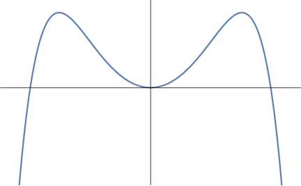 (ii)
(ii)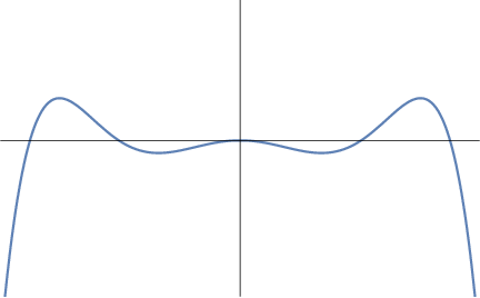 (iii)
(iii)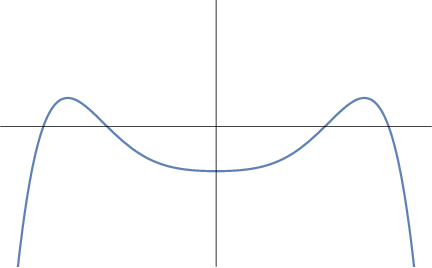
Therefore, by (34), the roots of are always . According to Proposition 2.2, to determine their correspondence with we must sort depending on the causal character of . By Proposition 2.2, the sorting is such that and whenever is null (in which case, by Remark 2.2, has an at least double root at zero and no negative roots) and when is non-null.
If , then zero is not a root of . Being the square root of the charateristic polynomial of (see (23)), this implies that has no zero eigenvalues. Thus and by Proposition 2.2, the conformal class of is given by:
- 1.a)
, and covering the region .
When it is straightforward to compute the kernel of . The result is
so the kernel is two-dimensional in this case. The pull-back of the scalar product on this space is
This is timelike if , null if and spacelike if . By (36), requires the vanishing of and/or , and by Proposition 2.2, the conformal class of is given by
- 1.b)
If , then and , , cover the region .
- 1.c)
If , then and , , cover the region .
- 1.d)
If , then and , , cover the region .
Case 2.
In this case the roots of are immediately found to be together with the double root . If it again follows that , thus the conformal class of is given by the parameters , covering the region . When the kernel of is
so the kernel is again two-dimensional and restricted to this space is
Thus, is timelike and the conformal class of is given by
- 2)
, covering the region .
Case 3.
In this case the roots of are also trivial. There is a double root at zero and another one at . Note that from the scaling freedom of (cf. (33)), is also defined up to a scaling factor and up to . Then the root can be scaled by a non-zero positive factor , which will be relevant to cover the maximal space of parameters in the space of conformal classes. Observe that (in any of the three cases) there is no restriction on the value of .
The kernel of the endomorphism is
hence four-dimensional and restricted to this space is
and the rest zero, and where we have written the constant curvature metric as
The kernel is now spacelike if , degenerate if and timelike if . Thus, for each case, the conformal class of is
- 3.a)
For , , covering the region .
- 3.b)
For , covering a single point.
- 3.c)
For , , covering the region .
Summarizing, the cases 1,2 and 3 correspond to CKVs and whose respective conformal classes cover the space of parameters
| (37) | ||||
| (38) |
By Proposition (2.2), corresponds to the entire space parameterizing the conformal classes of CKVs of conformally flat -metrics. Thus, we have proven that these metrics correspond exactly to all metrics in the five dimensional Kerr-de Sitter-like class. This, combined with Theorem 3.1, yields the following result:
Theorem 4.1.
In five spacetime dimensions, the following classes of -vacuum metrics are equivalent:
5 Discussion
We have obtained a method to determine the conformal class of an arbitrary CKV of a locally conformally flat metric of any dimension and signature. Such method is based on pointwise properties of the CKVs and it is independent on the coordinates and the representative of the class of metrics conformal to . This improves previously existing results (cf. [27, 29]) which require to find an explicitly flat representative in Cartesian coordinates.
Our result is stated as a computationally neat algorithm in Theorem 2.5, which allows for a straightforward application in Section 4. Namely, we classify the asymptotic data of all five-dimensional, algebraically special, -vacuum spacetimes, whose optical matrix is non-degenerate (cf. [4]). Such asymptotic data are determined by the conformal class of a CKV of a conformally flat . Furthermore, we prove equivalence of this collection of spacetimes with the Kerr-de Sitter-like class as well as with the -vacuum Kerr-Schild spacetimes satisfying a natural asymptotic condition (cf. Theorem 3.1).
It is worth commenting that the results of Section 4, besides providing an application of Theorem 2.5, outline the way for potential future results. As pointed out in [4], in dimensions higher than four, there exist several results (cf. [11, 31]) supporting the idea that the class of algebraically special solutions is more rigid than in four dimensions. One then wonders whether Theorem 3.1 also holds in any dimension higher than five. Surprisingly, the results in [4] do not rely on any asymptotic property of the spacetime, while in [29] it is central. Yet, the class of spacetimes studied [4] and in [29] (in five spacetime dimensions) happen to be equivalent, as we have shown in this paper. This hints a possible connection between asymptotic properties of spacetimes and the algebraic classification of the Weyl tensor. More precisely, the algebraically special condition with non-degenerate optical matrix implies conformal extendability with locally conformally flat . A better understanding of this aspect would be of substantial intrinsic interest and key for extending Theorem 3.1 to arbitrary dimensions.
It is also interesting to observe that the Weyl tensor of the spacetime determines, in any dimension, the Weyl tensor77 7 Note that and as defined in (25), are indeed independent objects at , however both obtainable from the spacetime Weyl tensor at . of the metric induced at . Indeed, an asymptotic expansion of , shows that its components fully tangent to coincide with to the leading order. The Weyl tensor contains a lot of information about the conformal class of metrics of dimension equal or higher than four88 8 The conformal class determines the Weyl tensor, but the opposite is not always true, cf. [18]., so it would not be surprising that the algebraically special condition on imposes strong conditions on the conformal class of (four or higher dimensional) . However, in four spacetime dimensions, is three dimensional and thus vanishes identically, so it is not clear in this case how the algebraic type of affects the conformal class of . The difference between the four and higher dimensional cases may be responsible for the lack of rigidity of algebraically special metrics in four dimensions, because recall (cf. Section 3) that the conformal class of is one of the freely speciable data in the asymptotic Cauchy problem. This, however, does not rule out other possible relations between the algebraic type of the four-dimensional spacetime metrics and their asymptotic properties. One connection may arise from the fact that the other component of the asymptotic data is, in four dimensions, the electric part of the rescaled Weyl tensor (cf. Section 3). In addition, constraints on the conformal class of may also appear as a consequence of the relation between and Cotton tensor of , which plays a similar role than the Weyl tensor for three dimensional metrics. These potential connections are worth to investigate in the future.
6 Acknowledgments
The authors wish to thank Igor Khavkine for comments on the manuscript and for providing useful references. MM acknowledges financial support under the projects PGC2018-096038-B-I00 (Spanish Ministerio de Ciencia, Innovación y Universidades and FEDER), SA096P20 (Junta de Castilla y León) and CPN is supported by the grant No 22-14791S of the Czech Science Foundation.
References
- [1] M. T. Anderson. Existence and stability of even-dimensional asymptotically de Sitter spaces. Annales Henri Poincaré, 6:801–820, 2005.
- [2] M. T. Anderson and P. T. Chruściel. Asymptotically simple solutions of the vacuum Einstein equations in even dimensions. Communications in Mathematical Physics, 260:557–577, 2005.
- [3] R. Beig and P. T. Chruściel. Killing initial data. Classical and Quantum Gravity, 14:83–92, 1997.
- [4] G. Bernardi de Freitas, M. Godazgar, and H. S. Reall. Uniqueness of the Kerr-de Sitter spacetime as an algebraically special solution in five dimensions. Communications in Mathematical Physics, 340:291–323, 2015.
- [5] G. Bernardi de Freitas, M. Godazgar, and H. S. Reall. Twisting algebraically special solutions in five dimensions. Classical and Quantum Gravity, 33:095002, 2016.
- [6] D. E. Blair. Inversion Theory and Conformal Mapping. Student Mathematical Library. American Mathematical Society, Providence, Rhode Island, 2000.
- [7] Y. Chen, and E. Teo. A new AF gravitational instanton. Physics Letters B, 703: 359-362, 2011.
- [8] A. Coley, R. Milson, V. Pravda, and A. Pravdová. Classification of the Weyl tensor in higher dimensions. Classical and Quantum Gravity, 21:35–41, 2004.
- [9] D. H. Collingwood and W. L. McGovern. Nilpotent orbits in semisimple Lie algebras. Van Nostrand Reinhold, New York 1993.
- [10] A. Derdzinski. Two-jets of conformal fields along their zero sets. Central European Journal of Mathematics, 10:1698–1709, 2012.
- [11] O. J. C. Dias and H. S. Reall. Algebraically special perturbations of the Schwarzschild solution in higher dimensions. Classical and Quantum Gravity, 30:095003, 2013.
- [12] C. Fefferman and C. R. Graham. Conformal invariants. Élie Cartan et les mathématiques d’aujourd’hui, S131: 95–116. Société mathématique de France, 1985.
- [13] C. Fefferman and C. R. Graham. The Ambient Metric, Annals of Mathematics Studies, 178. Princeton University Press, 2012.
- [14] H. Friedrich. On the regular and asymptotic characteristic initial value problem for Einstein’s vacuum field equations. Proceedings of the Royal Society of London A, 375:169–184, 1981.
- [15] H. Friedrich. The asymptotic characteristic initial value problem for Einstein’s vacuum field equations as an initial value problem for a first-order quasilinear symmetric hyperbolic system. Proceedings of the Royal Society of London A, 378:401–421, 1981.
- [16] H. Friedrich. On the existence of n-geodesically complete or future complete solutions of einstein’s field equations with smooth asymptotic structure. Communications in Mathematical Physics, 107:587–609, 1986.
- [17] G.W. Gibbons, H. Lü, D. N. Page, and C.N. Pope. The general Kerr–de Sitter metrics in all dimensions. Journal of Geometry and Physics, 53:49 – 73, 2005.
- [18] G. Hall. Some remarks on the converse of Weyl’s conformal theorem. Journal of Geometry and Physics, 60:1–7, 2010.
- [19] S. Hollands, A. Ishibashi, and D. Marolf. Comparison between various notions of conserved charges in asymptotically AdS spacetimes. Classical and Quantum Gravity, 22:2881–2920, 2005.
- [20] W. Kamiński. Well-posedness of the ambient metric equations and stability of even dimensional asymptotically de Sitter spacetimes, 2021. ArXiv:2108.08085.
- [21] S. Kichenassamy. On a conjecture of Fefferman and Graham. Advances in Mathematics, 184:268–288, 2004.
- [22] A.W. Knapp. Lie Groups Beyond an Introduction. Progress in Mathematics. Birkhäuser Boston, 2002.
- [23] M. Mars. A spacetime characterization of the Kerr metric. Classical and Quantum Gravity, 16:2507–2523, 1999.
- [24] M. Mars, T. T. Paetz, and J. M. M. Senovilla. Classification of Kerr–de Sitter-like spacetimes with conformally flat . Classical and Quantum Gravity, 34:095010, 2017.
- [25] M. Mars, T.T. Paetz, J. M. M. Senovilla, and W. Simon. Characterization of (asymptotically) Kerr–de Sitter-like spacetimes at null infinity. Classical and Quantum Gravity, 33:155001, 2016.
- [26] M. Mars and C. Peón-Nieto. Skew-symmetric endomorphisms in : a unified canonical form with applications to conformal geometry. Classical and Quantum Gravity, 38:035005, 2020.
- [27] M. Mars and C. Peón-Nieto. Free data at spacelike and characterization of Kerr-de Sitter in all dimensions. The European Physical Journal C, 81, 2021.
- [28] M. Mars and C. Peón-Nieto. Skew-symmetric endomorphisms in : a unified canonical form with applications to conformal geometry. Classical and Quantum Gravity, 38:125009, 2021.
- [29] M. Mars and C. Peón-Nieto. Classification of Kerr-de Sitter-like spacetimes with conformally flat in all dimensions. Physical Review D, 105:044027, 2022.
- [30] M. Mars and J. M. M. Senovilla. A spacetime characterization of the Kerr-NUT-(A)de Sitter and related metrics. Annales Henri Poincaré, 16:1509–1550, 2015.
- [31] M. Ortaggio, V. Pravda, A. Pravdová, and H. S. Reall. On a five-dimensional version of the Goldberg–Sachs theorem. Classical and Quantum Gravity, 29:205002, 2012.
- [32] M. Ortaggio, V. Pravda, and A. Pravdová. Algebraic classification of higher dimensional spacetimes based on null alignment. Classical and Quantum Gravity, 30:013001, 2012.
- [33] T. T. Paetz. Killing Initial Data on spacelike conformal boundaries. Journal of Geometry and Physics, 106:51 – 69, 2016.
- [34] M. Schottenloher. A Mathematical Introduction to Conformal Field Theory, Lecture Notes in Physics, 43. Springer, Berlin-Heidelberg, 2008.
- [35] W. Simon. Characterizations of the Kerr metric. General Relativity and Gravitation, 16:465–476, 1984.
- [36] J. A. Valiente-Kroon. Conformal methods in general relativity. Cambridge University Press, Cambridge, 2016.