跳到论文正文
W Papers独立论文阅读器 arXiv:2207.01361 论文正文 计算阅读时间 · 0%
引用这篇论文根据当前论文元数据生成,正式投稿前建议核对。


License: CC BY 4.0
arXiv:2207.01361v1 [math.NA] 04 Jul 2022

BDDC preconditioners for divergence free virtual element discretizations of the Stokes equations

Tommaso Bevilacqua Note: Dipartimento di matematica, Universitá degli studi di Milano, Via Saldini 50, 20133 Milano, Italy; e-mail: tommaso.bevilacqua@unimi.it    Simone Scacchi Note: Dipartimento di matematica, Universitá degli studi di Milano, Via Saldini 50, 20133 Milano, Italy; e-mail: simone.scacchi@unimi.it
Abstract

The Virtual Element Method (VEM) is a new family of numerical methods for the approximation of partial differential equations, where the geometry of the polytopal mesh elements can be very general. The aim of this article is to extend the balancing domain decomposition by constraints (BDDC) preconditioner to the solution of the saddle-point linear system arising from a VEM discretization of the two-dimensional Stokes equations. Under suitable hypotesis on the choice of the primal unknowns, the preconditioned linear system results symmetric and positive definite, thus the preconditioned conjugate gradient method can be used for its solution. We provide a theoretical convergence analysis estimating the condition number of the preconditioned linear system. Several numerical experiments validate the theoretical estimates, showing the scalability and quasi-optimality of the method proposed. Moreover, the solver exhibits a robust behavior with respect to the shape of the polygonal mesh elements. We also show that a faster convergence could be achieved with an easy to implement coarse space, slightly larger than the minimal one covered by the theory.

Keywords: Virtual element method, divergence free discretization, saddle-point linear system, domain decomposition preconditioner.

1 Introduction

The balancing domain decomposition by constraints (BDDC) preconditioner is an iterative substructuring method for the solution of partial differential equations (PDEs), that belongs to the class of nonoverlapping domain decomposition algorithms [24, 25]. BDDC, first introduced in [14] for elliptic problems, represents an evolution of the balancing Neumann-Neumann preconditioner [25]. We also remark that BDDC presents several features in common with the dual-primal finite element tearing and interconnecting (FETI-DP) algorithm. In particular, the BDDC and FETI-DP operators share almost the same eigenvalues [22, 8], thus they exhibit analogous convergence properties. Both BDDC and FETI-DP have been successfully developed for finite and spectral element discretizations of several physical problems governed by PDEs, see e.g. [19, 28, 15, 23]. In particular, regarding the Stokes equations, they have been studied in [21, 20]. In recent years, BDDC and FETI-DP algorithms have been also extended to various innovative discretizations techniques for PDEs, such as Mortar discretizations [18], discontinuous Galerkin methods [16, 11], isogeometric analysis [17, 27], weak Galerkin methods [26] and virtual element methods [4, 5].

The Virtual Element Method (VEM), introduced in the pioneering paper [2], represents a generalization of the finite element method (FEM), that can easily handle general polytopal meshes. The core idea behind VEM is to use approximated discrete bilinear forms, whose computation requires only the integration of polynomials on the element boundary and interior. The resulting discrete solution is conforming and the accuracy guaranteed by such discrete bilinear forms turns to be sufficient to achieve the correct order of convergence. The advantage of these methods is that they can be applied on a wide choice of general polygonal meshes without the need to integrate complex non-polynomial functions on the elements, keeping an high degree of accuracy.

In the VEM literature only a few studies have focused on the construction and analysis of preconditioners for VEM approximations of PDEs; see [1, 9, 10, 12]). BDDC for VEM discretizations of scalar elliptic problems have been first introduced in [4, 5] and then extended to mixed formulations of scalar elliptic equations in [13]. To our knowledge, the development of effective non-overlapping domain decomposition preconditioners for VEM discretizations of the Stokes equations is still an open problem.

The novelty of the present study is to develop a BDDC preconditioner for the divergence free VEM discretization of the two-dimensional Stokes equations introduced in [3]. Our algorithm represents an extension to VEM of the BDDC preconditioner proposed in [21] for FEM discretizations of the Stokes equations with discontinuous pressure spaces. We prove a convergence rate estimate of the preconditioned system, independent of the number of subdomains and polylogarithmic with respect to the ratio H/hH/h, where HH denotes the subdomain size and hh the mesh size. Such an estimate yields the scalability and quasi-optimality of the resulting algorithm. Several numerical tests confirm the theoretical estimate and show the robustness of the solver with respect to different polygonal meshes.

The paper is organized as follows: in Section 2 we introduce the continuous problem and its variational formulation; in Section 3 we describe the VEM discretization; in Section 4 we introduce the domain decomposition tecnique and the BDDC preconditioner; in Sections 5 and 6 we describe the theoretical aspects, while in Section 7 we report several numerical results; finally in Section 8 we draw the conclusions.

2 Continuous problem

Let Ω⊆ℝ2\Omega\subseteq\mathbb{R}^{2}, with Γ=∂Ω\Gamma=\partial\Omega, and consider the stationary Stokes problem on Ω\Omega with homogeneous Dirichet boundary conditions:

{Find ​(𝐮,p)​ such that−ν​𝚫​𝐮−∇p=𝐟 in ​Ωdiv ​𝐮=0 in ​Ω𝐮=0 on ​Γ,\begin{cases}\text{Find }(\mathbf{u},p)\text{ such that}\\ -\nu\mathbf{\Delta}\mathbf{u}-\nabla p=\mathbf{f}\qquad&\text{ in }\mathit{\Omega}\\ \text{div }\mathbf{u}=0\qquad&\text{ in }\mathit{\Omega}\\ \mathbf{u}=0\qquad&\text{ on }\mathit{\Gamma},\end{cases} (1)

where 𝐮\mathbf{u} and pp are the velocity and the pressure fields, respectively. Furthermore 𝚫\mathbf{\Delta}, div and ∇\mathbf{\nabla} denote the vector Laplacian, the divergence and the gradient operators. Finally, 𝐟\mathbf{f} represents the external force, while ν>0\nu>0 is the viscosity.

Let us consider the spaces:

𝐕:=[H01(Ω)]2,Q:=L02(Ω)={q∈L2(Ω)s.t.∫Ωq dΩ=0}\displaystyle\mathbf{V}:=[H^{1}_{0}(\mathit{\Omega})]^{2},\qquad Q:=L^{2}_{0}(\mathit{\Omega})=\bigg\{q\in L^{2}(\mathit{\Omega})\quad s.t.\quad\int_{\mathit{\Omega}}q\text{ d}\Omega=0\bigg\} (2)

with norms:

‖𝐯‖1:=‖𝐯‖[H1​(Ω)]2,‖q‖Q:=‖q‖L2​(Ω).\displaystyle\|\mathbf{v}\|_{1}:=\|\mathbf{v}\|_{[H^{1}(\mathit{\Omega})]^{2}},\quad\|q\|_{Q}:=\|q\|_{L^{2}(\mathit{\Omega})}. (3)

We assume 𝐟∈[H−1​(Ω)]2\mathbf{f}\in[H^{-1}(\mathit{\Omega})]^{2}, and ν∈L∞​(Ω)\nu\in L^{\infty}(\mathit{\Omega}) uniformly positive in Ω\mathit{\Omega}. Let the bilinear forms a⁡(⋅,⋅):𝐕×𝐕→ℝa(\cdot,\cdot):\mathbf{V}\times\mathbf{V}\rightarrow\mathbb{R} and b:𝐕×Q→ℝb:\mathbf{V}\times Q\rightarrow\mathbb{R} be defined as:

a(𝐮,𝐯):=∫Ων∇𝐮:∇𝐯 dΩfor all 𝐮,𝐯∈𝐕a(\mathbf{u},\mathbf{v}):=\int_{\Omega}\nu\mathbf{\nabla u}:\mathbf{\nabla v}\text{ d}\Omega\qquad\text{for all }\mathbf{u},\mathbf{v}\in\mathbf{V} (4)
b⁡(𝐯,q):=∫Ωdiv ​𝐯​q​ d​Ωfor all ​𝐮∈𝐕,q∈Q.b(\mathbf{v},q):=\int_{\Omega}\text{div }\mathbf{v}q\text{ d}\Omega\qquad\text{for all }\mathbf{u}\in\mathbf{V},q\in Q. (5)

Then a standard variational formulation of problem (1) reads:

{find ​(𝐮,p)∈𝐕×Q​ such thata⁡(𝐮,𝐯)+b⁡(𝐯,p)=(𝐟,𝐯)for all ​𝐯∈𝐕,b⁡(𝐮,q)=0for all ​q∈Q,\begin{cases}\text{find }(\mathbf{u},p)\in\mathbf{V}\times Q\text{ such that}\\ a(\mathbf{u},\mathbf{v})+b(\mathbf{v},p)=(\mathbf{f},\mathbf{v})&\text{for all }\mathbf{v}\in\mathbf{V},\\ b(\mathbf{u},q)=0&\text{for all }q\in Q,\end{cases} (6)

where

(𝐟,𝐯):=∫Ω𝐟⋅𝐯​ d​Ω.\displaystyle(\mathbf{f},\mathbf{v}):=\int_{\Omega}\mathbf{f}\cdot\mathbf{v}\text{ d}\Omega.

It is well-known that:

  • •

    a⁡(⋅,⋅)a(\cdot,\cdot) and b⁡(⋅,⋅)b(\cdot,\cdot) are continuous, i.e.

    |a⁡(𝐮,𝐯)|≤‖a‖​‖𝐮‖1​‖𝐯‖1for all ​𝐮,𝐯∈𝐕,|b⁡(𝐯,q)|≤‖b‖​‖𝐯‖1​‖q‖Qfor all ​𝐯∈𝐕​and ​q∈Q,\begin{array}[]{llll}|a(\mathbf{u},\mathbf{v})|&\leq&\|a\|\|\mathbf{u}\|_{1}\|\mathbf{v}\|_{1}&\quad\text{for all }\mathbf{u},\mathbf{v}\in\mathbf{V}\vskip 5.69046pt,\\ |b(\mathbf{v},q)|&\leq&\|b\|\|\mathbf{v}\|_{1}\|q\|_{Q}&\quad\text{for all }\mathbf{v}\in\mathbf{V}\text{and }q\in Q,\end{array}

    where ‖a‖\|a\| and ‖b‖\|b\| are the usual norm of the two bilinear forms;

  • •

    a⁡(⋅,⋅)a(\cdot,\cdot) is coercive i.e., there exists a positive constant α\alpha such that

    |a⁡(𝐯,𝐯)|≥α​‖𝐯‖12for all ​𝐯∈𝐕;|a(\mathbf{v},\mathbf{v})|\geq\alpha\|\mathbf{v}\|_{1}^{2}\quad\text{for all }\mathbf{v}\in\mathbf{V};
  • •

    the bilinear form b⁡(⋅,⋅)b(\cdot,\cdot) satisfies the inf-sup condition [6], i.e.

    ∃β>0​ such thatsup𝐯∈𝐕,𝐯≠𝟎|b⁡(𝐯,q)|‖𝐯‖1≥β​‖q‖Qfor all ​q∈Q.\exists\beta>0\text{ such that}\quad\sup_{\mathbf{v}\in\mathbf{V},\mathbf{v}\neq\mathbf{0}}\frac{|b(\mathbf{v},q)|}{\|\mathbf{v}\|_{1}}\geq\beta\|q\|_{Q}\quad\text{for all }q\in Q. (7)

Therefore, problem (6) has a unique solution (𝐮,p)∈𝐕×Q(\mathbf{u},p)\in\mathbf{V}\times Q such that

‖𝐮‖1+‖p‖Q≤C||𝐟||H−1​(Ω),\displaystyle||\mathbf{u}||_{1}+||p||_{Q}\leq C||\mathbf{f}||_{H^{-1}(\mathit{\Omega})}, (8)

where the constant CC depends only on Ω\mathit{\Omega} and ν\nu; see [6].

3 Virtual element discretization

We present here the discretization of problem (1), based on the virtual element space introduced in [3], that is designed to solve a Stokes-like problem element-wise. In particular we will use the reduced space presented in section 5 of [3], that, exploiting the divergence free property of the solution, allows to save a lot of degrees of freedom especially when the polynomial degree kk is large. We recall here the definition of the local spaces. Let {𝒯h}h\{{\mathcal{T}}_{h}\}_{h} be a sequence of triangulations of Ω\Omega into general polygonal elements KK with

hK:=diameter​(K),h:=supK∈𝒯hhK.\displaystyle h_{K}:=\text{diameter}(K),\quad h:=\sup_{K\in{\mathcal{T}}_{h}}h_{K}.

We suppose that, for all hh, each element K∈𝒯hK\in{\mathcal{T}}_{h} satisfies the following assumptions:

  • •

    (𝐀𝟏)(\mathbf{A1}) KK is star-shaped with respect to a ball of radius ≥γ​hk\geq\gamma h_{k},

  • •

    (𝐀𝟐)(\mathbf{A2}) the distance between any two vertices of K is ≥c​hK\geq ch_{K},

  • •

    (𝐀𝟑)(\mathbf{A3}) the triangulation 𝒯h{\mathcal{T}}_{h} is quasi-uniform, i.e. there exist positive constants c0,c1c_{0},\,c_{1} such that for any two elements KK and K′K^{\prime} in 𝒯h{\mathcal{T}}_{h} we have c0≤hK/hK′≤c1c_{0}\leq h_{K}/h_{K^{\prime}}\leq c_{1}.

where γ\gamma and cc are positive constants.

Remark 3.1.

These hypotheses could be weakened as in [2], for example assuming that every KK is a union of a finite (and uniformly bounded) number of star-shaped domains, each satisfying (𝐀𝟏\mathbf{A1}).

We also assume that the scalar viscosity field ν\nu is piecewise constant with respect to the decomposition 𝒯h{\mathcal{T}}_{h}, i.e. ν\nu is constant on each polygon K∈𝒯hK\in{\mathcal{T}}_{h}.

For k∈ℕk\in\mathbb{N}, let us define the spaces:

  • •

    ℙk​(K)\mathbb{P}_{k}(K) the set of polynomials on KK of degree ≤k\leq k,

  • •

    𝔹k(K):={v∈C0(∂K) s.t. v|e∈ℙk(e)∀ edge e∈∂K}\mathbb{B}_{k}(K):=\{v\in C^{0}(\partial K)\text{ s.t. }v_{|e}\in\mathbb{P}_{k}(e)\quad\forall\text{ edge }e\in\partial K\},

  • •

    Gk​(K):=∇(ℙk+1​(K))⊆[ℙk​(K)]2\mathit{G}_{k}(K):=\nabla(\mathbb{P}_{k+1}(K))\subseteq[\mathbb{P}_{k}(K)]^{2},

  • •

    Gk​(K)⟂⊆[ℙk​(K)]2\mathit{G}_{k}(K)^{\perp}\subseteq[\mathbb{P}_{k}(K)]^{2} the L2L^{2}-orthogonal complement to Gk​(K)\mathit{G}_{k}(K).

On each element K∈ThK\in\mathit{T}_{h} we define, for k≥2k\geq 2, the following finite dimensional local virtual element spaces:

𝐕^hK:={𝐯∈[H1(K)]2 s.t. 𝐯|∂K∈𝔹k(∂K)]2,{−ν​𝚫​𝐯−∇s∈Gk−2​(K)⟂,div ​𝐯∈ℙ0​(K),for some s∈L2(K)}\begin{split}\mathbf{\widehat{V}}_{h}^{K}:=\bigg\{\mathbf{v}\in[H^{1}(K)]^{2}\text{ s.t. }\mathbf{v}_{|\partial K}\in\mathbb{B}_{k}(\partial K)]^{2},\\ \begin{cases}-\nu\mathbf{\Delta}\mathbf{v}-\nabla s\in\mathit{G}_{k-2}(K)^{\perp},\\ \text{div }\mathbf{v}\in\mathbb{P}_{0}(K),\end{cases}\text{for some }s\in L^{2}(K)\bigg\}\end{split} (9)

and

QhK:=ℙ0​(K).\displaystyle Q_{h}^{K}:=\mathbb{P}_{0}(K). (10)

Now it is possible to introduce suitable sets of degrees of freedom for the local approximations fields.
Given a function 𝐯∈𝐕^hK\mathbf{v}\in\mathbf{\widehat{V}}_{h}^{K} we take the following linear operators 𝐃𝐕^\mathbf{D_{\widehat{V}}}, split into three subsets:

  • •

    𝐃𝐕^​𝟏\mathbf{D_{\widehat{V}}1}: the values of 𝐯\mathbf{v} at the vertices of the polygon KK,

  • •

    𝐃𝐕^​𝟐\mathbf{D_{\widehat{V}}2}: the values of 𝐯\mathbf{v} at k−1k-1 distinct points of every edge e∈∂Ke\in\partial K (for the implementation we will take the k−1k-1 internal points of the (k+1)(k+1)-Gauss-Lobatto quadrature rule in ee),

  • •

    𝐃𝐕^​𝟑\mathbf{D_{\widehat{V}}3}: the moments of the values of 𝐯\mathbf{v}

    ∫K𝐯⋅𝐠k−2⟂​ d​Kfor all ​𝐠k−2⟂∈𝐆k−2​(K)⟂\displaystyle\int_{K}\mathbf{v}\cdot\mathbf{g}^{\perp}_{k-2}\text{ d}K\qquad\text{for all }\mathbf{g}^{\perp}_{k-2}\in\mathbf{G}_{k-2}(K)^{\perp}

Furthermore, for the local pressure, given q∈QhKq\in Q^{K}_{h}, we consider the linear operators 𝐃𝐐\mathbf{D_{Q}}:

  • •

    𝐃𝐐\mathbf{D_{Q}}: the moment

    ∫Kq​ d​K.\displaystyle\int_{K}q\text{ d}K.

Since 𝐃𝐕^\mathbf{D_{\widehat{V}}} and 𝐃𝐐\mathbf{D_{Q}} are unisolvent respectively of 𝐕^hK\mathbf{\widehat{V}}_{h}^{K} and QhKQ_{h}^{K}, we can define the global virtual element spaces:

𝐕^h:={𝐯∈[H01(Ω)]2s.t.𝐯|K∈𝐕^hKfor all K∈𝒯h}\displaystyle\mathbf{\widehat{V}}_{h}:=\{\mathbf{v}\in[H^{1}_{0}(\mathit{\Omega})]^{2}\quad\text{s.t.}\quad\mathbf{v}_{|K}\in\mathbf{\widehat{V}}^{K}_{h}\quad\text{for all }K\in{\mathcal{T}}_{h}\} (11)

and

Qh:={q∈L02(Ω)s.t.q|K∈QhKfor all K∈𝒯h},\displaystyle Q_{h}:=\{q\in L^{2}_{0}(\mathit{\Omega})\quad\text{s.t.}\quad q_{|K}\in Q^{K}_{h}\quad\text{for all }K\in{\mathcal{T}}_{h}\}, (12)

with obvious associated sets of global degrees of freedom.

3.1 Discrete problem

Referring to [3], we can now state the discrete virtual element problem

{find ​(𝐮h,ph)​ such thatah​(𝐮h,𝐯h)+b⁡(𝐯h,ph)=(𝐟h,𝐯h)for all ​𝐯h∈𝐕^hb⁡(𝐮h,qh)=0for all ​qh∈Qh\begin{cases}\text{find }(\mathbf{u}_{h},p_{h})\text{ such that}\\ a_{h}(\mathbf{u}_{h},\mathbf{v}_{h})+b(\mathbf{v}_{h},p_{h})=(\mathbf{f}_{h},\mathbf{v}_{h})&\quad\text{for all }\mathbf{v}_{h}\in\mathbf{\widehat{V}}_{h}\\ b(\mathbf{u}_{h},q_{h})=0&\quad\text{for all }q_{h}\in Q_{h}\end{cases} (13)

By construction the discrete bilinear form ah​(⋅,⋅)a_{h}(\cdot,\cdot) is stable (uniformly) with respect to the 𝐕\mathbf{V} norm and also obviously the bilinear form b⁡(⋅,⋅)b(\cdot,\cdot). Therefore, to prove the existence and uniqueness of the solution of the problem (13) is necessary only a suitable inf-sup condition. For our work, we will only need this condition for the subdomains in which Ω\Omega will be divided into. In this way the local subdomains problem, as weel as the global one, will be well posed. The proof of the following inf-sup condition could be found in [3].

Proposition 3.1.

Given the discrete spaces 𝐕^h\mathbf{\widehat{V}}_{h} and QhQ_{h} defined in (11) and (12), there exists a positive β~\tilde{\beta}, independent of h, such that:

sup𝐯h∈𝐕^h,𝐯h≠𝟎|b⁡(𝐯h,qh)|‖𝐯h‖1≥β~​‖qh‖Qfor all ​qh∈Qh.\sup_{\mathbf{v}_{h}\in\mathbf{\widehat{V}}_{h},\mathbf{v}_{h}\neq\mathbf{0}}\frac{|b(\mathbf{v}_{h},q_{h})|}{\|\mathbf{v}_{h}\|_{1}}\geq\tilde{\beta}\|q_{h}\|_{Q}\quad\text{for all }q_{h}\in Q_{h}. (14)

A consequence of the previous proposition is the following statement.

Theorem 3.1.

Problem (13) has a unique solution (𝐮h,ph)∈𝐕^h×Qh(\mathbf{u}_{h},p_{h})\in\mathbf{\widehat{V}}_{h}\times Q_{h}, verifying the estimate

‖𝐮h‖1+‖ph‖Q≤C​‖𝐟‖0​.\displaystyle\|\mathbf{u}_{h}\|_{1}+\|p_{h}\|_{Q}\leq C\|\mathbf{f}\|_{0}\text{.} (15)

We have also a convergence result

Theorem 3.2.

Let (𝐮,p)∈𝐕×Q(\mathbf{u},p)\in\mathbf{V}\times Q be the solution of problem (6) and (𝐮h,ph)∈𝐕^h×Qh(\mathbf{u}_{h},p_{h})\in\mathbf{\widehat{V}}_{h}\times Q_{h} be the solution of problem (13). Then it holds

‖𝐮−𝐮h‖1≤C​hk​(|𝐟|k−1+|​𝐮|k+1)\displaystyle\|\mathbf{u}-\mathbf{u}_{h}\|_{1}\leq Ch^{k}(|\mathbf{f}|_{k-1}+|\mathbf{u}|_{k+1}) (16)

and

‖p−ph‖Q≤C​hk​(|𝐟|k−1+|𝐮|k+1+|​p|k)​.\displaystyle\|p-p_{h}\|_{Q}\leq Ch^{k}(|\mathbf{f}|_{k-1}+|\mathbf{u}|_{k+1}+|p|_{k})\text{.} (17)

4 Construction of the BDDC preconditioner

In this section, we first divide the domain Ω\Omega into subdomains and introduce appropriate function spaces, paragraph 4.1. Then, in paragraph 4.2, we show how the global interface saddle-point problem takes form and then in 4.3 we define the BDDC preconditioner that allows us to use a preconditioned conjugate gradient method (PCG) for its solution.

4.1 Domain decomposition

We decompose the domain Ω\Omega into NN non-overlapping subdomains Ωi,i=1,2,…​N\Omega_{i},i=1,2,...N, of characteristic diameter HH. Each subdomain is a union of shape regular elements and the nodes on the boundaries of neighboring subdomain match across the interface Γ=(∪∂Ωi)∖∂Ω\Gamma=(\cup\partial\Omega_{i})\setminus\partial\Omega; we define also Γi=∂Ωi∩Γ\Gamma_{i}=\partial\Omega_{i}\cap\Gamma as the interface of an individual subdomain Ωi\Omega_{i}. According to [5], where more details could be found, we recall two requirements on the subdomain partition:

  • •

    (S1) Each subdomain Ωi\Omega_{i} is the union of polygonal elements of the triangulation 𝒯h{\mathcal{T}}_{h} and the number of polygons forming an individual subdomain is uniformly bounded;

  • •

    (S2) If a face of a subdomain intersects ∂Ω\partial\Omega, then the measure of this set is comparable to that of ∂Ωi\partial\Omega_{i}. Similarly, if an edge of a subdomain intersects ∂Ω\partial\Omega, the length of this intersection is bounded from below in terms of the diameter of ∂Ωi\partial\Omega_{i}.

Refer to caption
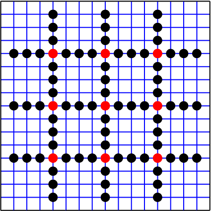
Figure 1: Interface of the subdomains (excluding the nodes on the boundary): red circles indicate the vertices of the subdomains, whereas black circles indicate the remainder interface nodes.

Restricting to the two-dimensional case, although the theory of iterative substructuring ([25] Section 4.2) does not cover the general cases where the boundary of a subdomain is not a straight line (as we have in our implementation, since we use general polygonal meshes), we can anyway define vertices and interface relatively easily. We say that a node xx belongs to the interface of a subdomain if it belongs to at least two subdomains, while a node xx is a vertex of a subdomain if it belongs to more than two subdomains (Figure 1). This is the rule that we used in the implementation to split our mesh in the different subdomains.

4.2 Decomposition of the virtual element spaces

The discrete variational problem (13) can be written, in matrix form, as the following saddle-point linear system:

[ABTB0]​[𝐮p]=[𝐟0]\left[\begin{array}[]{cc}A&B^{T}\\ B&0\\ \end{array}\right]\left[\begin{array}[]{c}\mathbf{u}\\ p\\ \end{array}\right]=\left[\begin{array}[]{c}\mathbf{f}\\ 0\\ \end{array}\right] (18)

where the matrices A and B are associated with the discrete bilinear forms ah​(⋅,⋅)a_{h}(\cdot,\cdot) and b⁡(⋅,⋅)b(\cdot,\cdot). In the remainder of the paper, we omit the underscore hh since we will always refer to the finite dimensional space and so we write 𝐕^×Q\mathbf{\widehat{V}}\times Q instead of 𝐕^h×Qh\mathbf{\widehat{V}}_{h}\times Q_{h}, only for sake of simplifying the notation. Referring to the notations of the previous section, we naturally split the degrees of freedom (dofs) of the velocity components into boundary dofs (𝐃𝐕​𝟏\mathbf{D_{V}1} and 𝐃𝐕​𝟐\mathbf{D_{V}2}) and interior dofs (𝐃𝐕​𝟑\mathbf{D_{V}3} and 𝐃𝐕​𝟒\mathbf{D_{V}4}). Following the notations introduced in [21], we decompose the discrete velocity and pressure space 𝐕^\mathbf{\widehat{V}} and QQ into:

𝐕^=𝐕I​⨁𝐕^Γ​,Q=QI​⨁Q0​.\mathbf{\widehat{V}}=\mathbf{V}_{I}\bigoplus\mathbf{\widehat{V}}_{\Gamma}\text{,}\quad Q=Q_{I}\bigoplus Q_{0}\text{.} (19)

𝐕I\mathbf{V}_{I} and QIQ_{I} are direct sums of subdomain interior velocity spaces 𝐕I(i)\mathbf{V}_{I}^{(i)}, and subdomain interior pressure spaces QI(i)Q_{I}^{(i)}, respectively, i.e.,

𝐕I=⨁i=1N𝐕I(i)​,QI=⨁i=1NQI(i)​.\mathbf{V}_{I}=\bigoplus_{i=1}^{N}\mathbf{V}_{I}^{(i)}\text{,}\quad Q_{I}=\bigoplus_{i=1}^{N}Q_{I}^{(i)}\text{.} (20)

The elements of 𝐕I(i)\mathbf{V}_{I}^{(i)} have support in the subdomain Ωi\Omega_{i} and vanish on its interface Γi\Gamma_{i}, while the elements of QI(i)Q_{I}^{(i)} are restrictions of elements in Q to Ωi\Omega_{i}. 𝐕^Γ\mathbf{\widehat{V}}_{\Gamma} is the space of the traces on Γ\Gamma of functions in 𝐕^\mathbf{\widehat{V}} and Q0Q_{0} is the subspace of QQ with constant values q0(i)q_{0}^{(i)} in the subdomain Ωi\Omega_{i}. We denote the space of interface velocity variables of the subdomain Ωi\Omega_{i} by 𝐕Γ(i)\mathbf{V}_{\Gamma}^{(i)}, and the associated product space by 𝐕Γ=∏i=1N𝐕Γ(i)\mathbf{V}_{\Gamma}=\prod_{i=1}^{N}\mathbf{V}_{\Gamma}^{(i)}; generally functions in 𝐕Γ\mathbf{V}_{\Gamma} are discontinuous across the interface. RΓ(i):𝐕^Γ→𝐕Γ(i)R_{\Gamma}^{(i)}:\mathbf{\widehat{V}}_{\Gamma}\rightarrow\mathbf{V}_{\Gamma}^{(i)} is the operator which maps functions in the continuous interface velocity space 𝐕^Γ\mathbf{\widehat{V}}_{\Gamma} to their subdomain components in the space 𝐕Γ(i)\mathbf{V}_{\Gamma}^{(i)}. We denote the direct sum of the RΓ(i)R_{\Gamma}^{(i)} with RΓR_{\Gamma}.
With the decomposition of the solution space given in (19), the global saddle-point problem (18) can be written as: find (𝐮I,pI,𝐮Γ,p0)∈(𝐕I,QI,𝐕^Γ,Q0)(\mathbf{u}_{I},p_{I},\mathbf{u}_{\Gamma},p_{0})\in(\mathbf{V}_{I},Q_{I},\mathbf{\widehat{V}}_{\Gamma},Q_{0}), such that:

[AI​IBI​ITA^Γ​IT0BI​I0B^I​Γ0A^Γ​IB^I​ΓTA^Γ​ΓB^0​ΓT00B^0​ΓT0]​[𝐮IpI𝐮Γp0]=[𝐟I0𝐟Γ0].\left[\begin{array}[]{cccc}A_{II}&B_{II}^{T}&\widehat{A}_{\Gamma I}^{T}&0\\ B_{II}&0&\widehat{B}_{I\Gamma}&0\\ \widehat{A}_{\Gamma I}&\widehat{B}_{I\Gamma}^{T}&\widehat{A}_{\Gamma\Gamma}&\widehat{B}_{0\Gamma}^{T}\\ 0&0&\widehat{B}_{0\Gamma}^{T}&0\\ \end{array}\right]\left[\begin{array}[]{c}\mathbf{u}_{I}\\ p_{I}\\ \mathbf{u}_{\Gamma}\\ p_{0}\\ \end{array}\right]=\left[\begin{array}[]{c}\mathbf{f}_{I}\\ 0\\ \mathbf{f}_{\Gamma}\\ 0\\ \end{array}\right]. (21)
Remark 4.1.

Here the lower left block of (21) is zero because the bilinear form b⁡(𝐮I,q0)b(\mathbf{u}_{I},q_{0}) vanishes for any 𝐯I∈𝐕I\mathbf{v}_{I}\in\mathbf{V}_{I} and q0∈Q0q_{0}\in Q_{0}. To keep this property, when the change of basis for the pressure space is applied, it is important to take care of the fact that the shape and dimension of the elements is different.

The blocks related to the continuous interface velocity are assembled from the corresponding subdomain submatrices, e.g., A^Γ​Γ=∑i=1NRΓ(i)T​A^Γ​Γ(i)​RΓ(i)\widehat{A}_{\Gamma\Gamma}=\sum_{i=1}^{N}{R_{\Gamma}^{(i)}}^{T}\widehat{A}_{\Gamma\Gamma}^{(i)}R_{\Gamma}^{(i)} and B^0​Γ=∑i=1NB^0​Γ(i)​RΓ(i)\widehat{B}_{0\Gamma}=\sum_{i=1}^{N}\widehat{B}_{0\Gamma}^{(i)}R_{\Gamma}^{(i)}. Correspondingly, the right-hand side vector 𝐟I\mathbf{f}_{I} consists of subdomain vectors 𝐟I(i)\mathbf{f}_{I}^{(i)}, and 𝐟Γ\mathbf{f}_{\Gamma} is assembled from the subdomain components 𝐟Γ(i)\mathbf{f}_{\Gamma}^{(i)}; we denote the spaces of the right-hand side vectors 𝐟I\mathbf{f}_{I} and 𝐟Γ\mathbf{f}_{\Gamma} by 𝐅I\mathbf{F}_{I} and 𝐅Γ\mathbf{F}_{\Gamma} respectively.

By employing a symmetric permutation, the leading two by two blocks in the coefficient matrix can be rewritten as a block diagonal matrix with blocks corresponding to independent subdomain problems. We show here how such a matrix takes form in the simplest case of two subdomains:

[AI​I(1)BI​I(1)T00AΓ​I(1)T0BI​I(1)000BI​Γ(1)000AI​I(2)BI​I(2)TAΓ​I(2)T000BI​I(2)0BI​Γ(2)0AΓ​I(1)BI​Γ(1)TAΓ​I(2)BI​Γ(2)TA^Γ​ΓB^0​ΓT0000B^0​Γ0]​[𝐮I(1)pI(1)𝐮I(2)pI(2)𝐮Γp0]=[𝐟I(1)0𝐟I(2)0𝐟Γ0].\left[\begin{array}[]{cccccc}A_{II}^{(1)}&{B_{II}^{(1)}}^{T}&0&0&{A_{\Gamma I}^{(1)}}^{T}&0\\ B_{II}^{(1)}&0&0&0&B_{I\Gamma}^{(1)}&0\\ 0&0&A_{II}^{(2)}&{B_{II}^{(2)}}^{T}&{A_{\Gamma I}^{(2)}}^{T}&0\\ 0&0&B_{II}^{(2)}&0&B_{I\Gamma}^{(2)}&0\\ A_{\Gamma I}^{(1)}&{B_{I\Gamma}^{(1)}}^{T}&A_{\Gamma I}^{(2)}&{B_{I\Gamma}^{(2)}}^{T}&\widehat{A}_{\Gamma\Gamma}&{\widehat{B}_{0\Gamma}}^{T}\\ 0&0&0&0&\widehat{B}_{0\Gamma}&0\end{array}\right]\left[\begin{array}[]{c}\mathbf{u}_{I}^{(1)}\\ p_{I}^{(1)}\\ \mathbf{u}_{I}^{(2)}\\ p_{I}^{(2)}\\ \mathbf{u}_{\Gamma}\\ p_{0}\\ \end{array}\right]=\left[\begin{array}[]{c}\mathbf{f}_{I}^{(1)}\\ 0\\ \mathbf{f}_{I}^{(2)}\\ 0\\ \mathbf{f}_{\Gamma}\\ 0\\ \end{array}\right]. (22)

In the rest of this section the computations are always performed in the case of two subdomains. The extension to the general case with more subdomains is natural, but the computations are clearly more involved.
We proceed eliminating, by static condensation, the independent subdomain variables (𝐮I(1),pI(1))(\mathbf{u}_{I}^{(1)},p_{I}^{(1)}) and (𝐮I(2),pI(2))(\mathbf{u}_{I}^{(2)},p_{I}^{(2)}) in the system (22). To do so, we solve two independent Dirichlet problems:

[AI​I(1)BI​I(1)TBI​I(1)0]​[𝐮I(1)pI(1)]+[AΓ​I(1)T0BI​Γ(1)0]​[𝐮Γp0]=[𝐅I(1)0]​,\left[\begin{array}[]{cc}A_{II}^{(1)}&{B_{II}^{(1)}}^{T}\\ B_{II}^{(1)}&0\end{array}\right]\left[\begin{array}[]{c}\mathbf{u}_{I}^{(1)}\\ p_{I}^{(1)}\\ \end{array}\right]+\left[\begin{array}[]{cc}{A_{\Gamma I}^{(1)}}^{T}&0\\ B_{I\Gamma}^{(1)}&0\end{array}\right]\left[\begin{array}[]{c}\mathbf{u}_{\Gamma}\\ p_{0}\\ \end{array}\right]=\left[\begin{array}[]{c}\mathbf{F}_{I}^{(1)}\\ 0\\ \end{array}\right]\text{,} (23)
[AI​I(2)BI​I(2)TBI​I(2)0]​[𝐮I(2)pI(2)]+[AΓ​I(2)T0BI​Γ(2)0]​[𝐮Γp0]=[𝐅I(2)0]​,\displaystyle\left[\begin{array}[]{cc}A_{II}^{(2)}&{B_{II}^{(2)}}^{T}\\ B_{II}^{(2)}&0\end{array}\right]\left[\begin{array}[]{c}\mathbf{u}_{I}^{(2)}\\ p_{I}^{(2)}\\ \end{array}\right]+\left[\begin{array}[]{cc}{A_{\Gamma I}^{(2)}}^{T}&0\\ B_{I\Gamma}^{(2)}&0\end{array}\right]\left[\begin{array}[]{c}\mathbf{u}_{\Gamma}\\ p_{0}\\ \end{array}\right]=\left[\begin{array}[]{c}\mathbf{F}_{I}^{(2)}\\ 0\\ \end{array}\right]\text{,}

thus

[𝐮I(1)pI(1)]=[AI​I(1)BI​I(1)TBI​I(1)0]−1​([𝐅I(1)0]−[AΓ​I(1)T0BI​Γ(1)0]​[𝐮Γp0])​,\left[\begin{array}[]{c}\mathbf{u}_{I}^{(1)}\\ p_{I}^{(1)}\\ \end{array}\right]=\left[\begin{array}[]{cc}A_{II}^{(1)}&{B_{II}^{(1)}}^{T}\\ B_{II}^{(1)}&0\end{array}\right]^{-1}\left(\left[\begin{array}[]{c}\mathbf{F}_{I}^{(1)}\\ 0\\ \end{array}\right]-\left[\begin{array}[]{cc}{A_{\Gamma I}^{(1)}}^{T}&0\\ B_{I\Gamma}^{(1)}&0\end{array}\right]\left[\begin{array}[]{c}\mathbf{u}_{\Gamma}\\ p_{0}\\ \end{array}\right]\right)\text{,} (34)
[𝐮I(2)pI(2)]=[AI​I(2)BI​I(2)TBI​I(2)0]−1​([𝐅I(2)0]−[AΓ​I(2)T0BI​Γ(2)0]​[𝐮Γp0])​,\left[\begin{array}[]{c}\mathbf{u}_{I}^{(2)}\\ p_{I}^{(2)}\\ \end{array}\right]=\left[\begin{array}[]{cc}A_{II}^{(2)}&{B_{II}^{(2)}}^{T}\\ B_{II}^{(2)}&0\end{array}\right]^{-1}\left(\left[\begin{array}[]{c}\mathbf{F}_{I}^{(2)}\\ 0\\ \end{array}\right]-\left[\begin{array}[]{cc}{A_{\Gamma I}^{(2)}}^{T}&0\\ B_{I\Gamma}^{(2)}&0\end{array}\right]\left[\begin{array}[]{c}\mathbf{u}_{\Gamma}\\ p_{0}\\ \end{array}\right]\right)\text{,} (35)

Then, substituting the solutions of (34) and (35) in

[AΓ​I(1)BI​Γ(1)T00]​[𝐮I(1)pI(1)]+[AΓ​I(2)BI​Γ(2)T00]​[𝐮I(2)pI(2)]+[A^Γ​ΓB^0​ΓTB^0​Γ0]​[𝐮Γp0]=[𝐅Γ0]\left[\begin{array}[]{cc}A_{\Gamma I}^{(1)}&{B_{I\Gamma}^{(1)}}^{T}\\ 0&0\end{array}\right]\left[\begin{array}[]{c}\mathbf{u}_{I}^{(1)}\\ p_{I}^{(1)}\\ \end{array}\right]+\left[\begin{array}[]{cc}A_{\Gamma I}^{(2)}&{B_{I\Gamma}^{(2)}}^{T}\\ 0&0\end{array}\right]\left[\begin{array}[]{c}\mathbf{u}_{I}^{(2)}\\ p_{I}^{(2)}\\ \end{array}\right]+\left[\begin{array}[]{cc}\widehat{A}_{\Gamma\Gamma}&{\widehat{B}_{0\Gamma}}^{T}\\ \widehat{B}_{0\Gamma}&0\end{array}\right]\left[\begin{array}[]{c}\mathbf{u}_{\Gamma}\\ p_{0}\\ \end{array}\right]=\left[\begin{array}[]{c}\mathbf{F}_{\Gamma}\\ 0\\ \end{array}\right] (36)

we obtain the global interface saddle-point problem:

S^ u^=[S^ΓB^0​ΓTB^0​Γ0][𝐮Γp0]=[𝐠Γ0]=𝐠^,\widehat{S}\text{ }\widehat{u}=\left[\begin{array}[]{cc}\widehat{S}_{\Gamma}&{\widehat{B}_{0\Gamma}}^{T}\\ \widehat{B}_{0\Gamma}&0\\ \end{array}\right]\left[\begin{array}[]{c}\mathbf{u}_{\Gamma}\\ p_{0}\\ \end{array}\right]=\left[\begin{array}[]{c}\mathbf{g}_{\Gamma}\\ 0\\ \end{array}\right]=\widehat{\mathbf{g}}\text{,} (37)

where the right-hand side 𝐠^∈𝐅Γ×F0\widehat{\mathbf{g}}\in\mathbf{F}_{\Gamma}\times F_{0} is given by

𝐠^=∑i=12RΓ(i)T​{[𝐟Γ(i)0]−[AΓ​I(i)BI​Γ(i)T00]​[AI​I(i)BI​I(i)TBI​I(i)0]−1​[𝐟I(i)0]}.\displaystyle\widehat{\mathbf{g}}=\sum_{i=1}^{2}{R_{\Gamma}^{(i)}}^{T}\bigg\{\left[\begin{array}[]{c}\mathbf{f}_{\Gamma}^{(i)}\\ 0\\ \end{array}\right]-\left[\begin{array}[]{cc}A_{\Gamma I}^{(i)}&{B_{I\Gamma}^{(i)}}^{T}\\ 0&0\end{array}\right]\left[\begin{array}[]{cc}A_{II}^{(i)}&{B_{II}^{(i)}}^{T}\\ B_{II}^{(i)}&0\end{array}\right]^{-1}\left[\begin{array}[]{c}\mathbf{f}_{I}^{(i)}\\ 0\\ \end{array}\right]\bigg\}.

We note that S^\widehat{S} is assembled from the subdomain Stokes Schur complements S(i)S^{(i)}, which are defined by: given 𝐰(i)=𝐰Γ(i)×q0(i)∈𝐕Γ(i)×Q0(i){\mathbf{w}}^{(i)}=\mathbf{w}_{\Gamma}^{(i)}\times q_{0}^{(i)}\in\mathbf{V}_{\Gamma}^{(i)}\times Q_{0}^{(i)}, determine S(i)​𝐰(i)∈𝐅Γ(i)×F0(i)S^{(i)}{\mathbf{w}}^{(i)}\in\mathbf{F}_{\Gamma}^{(i)}\times F_{0}^{(i)} such that

[AI​I(i)BI​I(i)TAΓ​I(i)T0BI​I(i)0BI​Γ(i)0AΓ​I(i)BI​Γ(i)TAΓ​Γ(i)B0​Γ(i)T00B0​Γ(i)0]​[𝐰I(i)qI(i)𝐰Γ(i)q0(i)]=[𝟎0S(i)​𝐰(i)]​.\left[\begin{array}[]{cccc}A_{II}^{(i)}&{B_{II}^{(i)}}^{T}&{A_{\Gamma I}^{(i)}}^{T}&0\\ B_{II}^{(i)}&0&B_{I\Gamma}^{(i)}&0\\ A_{\Gamma I}^{(i)}&{B_{I\Gamma}^{(i)}}^{T}&{A}_{\Gamma\Gamma}^{(i)}&{{B}_{0\Gamma}^{(i)}}^{T}\\ 0&0&{B}_{0\Gamma}^{(i)}&0\end{array}\right]\left[\begin{array}[]{c}\mathbf{w}_{I}^{(i)}\\ q_{I}^{(i)}\\ \mathbf{w}_{\Gamma}^{(i)}\\ q_{0}^{(i)}\end{array}\right]=\left[\begin{array}[]{c}\mathbf{0}\\ 0\\ S^{(i)}{\mathbf{w}}^{(i)}\end{array}\right]\text{.} (46)

Denoting by SΓS_{\Gamma} the direct sum of the SΓ(i)S^{(i)}_{\Gamma}, then S^Γ\widehat{S}_{\Gamma} is given by

S^Γ=RΓT​SΓ​RΓ=∑i=12RΓ(i)T​SΓ(i)​RΓ(i),\widehat{S}_{\Gamma}=R_{\Gamma}^{T}S_{\Gamma}R_{\Gamma}=\sum_{i=1}^{2}{R^{(i)}_{\Gamma}}^{T}S^{(i)}_{\Gamma}R^{(i)}_{\Gamma}, (47)

and then we set

R=[RΓ00I]​,R(i)=[RΓ(i)00I]​.R=\left[\begin{array}[]{cc}R_{\Gamma}&0\\ 0&I\end{array}\right]\text{,}\quad R^{(i)}=\left[\begin{array}[]{cc}R_{\Gamma}^{(i)}&0\\ 0&I\end{array}\right]\text{.} (48)

Finally we see from (46), that the action of S(i)S^{(i)} on a vector can be evaluated by solving a Dirichlet problem on the subdomain Ωi\Omega_{i} as in (34) and (35), so it is not necessary to assemble the matrix S^\widehat{S} because only its action is required.
In the next section we introduce a BDDC preconditioner for problem (37), where the operator of the preconditioned problem is symmetric and positive definite, so we will use the PCG method to solve it.

4.3 BDDC preconditioner

We now present the BDDC preconditioner, first designed in [21] for finite element discretizations of the Stokes equations, that we will extend to the VEM discretization introduced in the previous sections. This preconditioner is very similar to FETI-DP, but there is a main difference between them: while in a FETI-DP algorithm the continuity of the solution will not be fully satisfied until the algorithm has converged, in the BDDC one full continuity is restored at the end of each iteration step, by using an average operator.
Before entering into the definition of the function space used to construct the BDDC preconditioner, we briefly justify the choice of our notation. The subscript Γ\Gamma indicates dofs living on the interface, Π\Pi and Δ\Delta are instead used to distinguish dofs of Γ\Gamma that belong to the primal and dual spaces, respectively, defined here below. Two other subscripts are used: CC indicates an operator referred to the coarse space and DD is instead used to highlight that an operator has been rescaled by suitable scaling functions, defined later. The hat ⋅^\widehat{\cdot} refers to a continuous space, the ⋅~\widetilde{\cdot} means that the space is continuous on primal interface dofs and discontinuous on the dual ones and finally no hat is used for the product of local spaces, which is discontinuous at all interface dofs.
As a first step, we introduce a partially assembled interface velocity space 𝐕~Γ\mathbf{\widetilde{V}}_{\Gamma},

𝐕~Γ=𝐕^Π​⨁𝐕Δ=𝐕^Π​⨁(∏i=1N𝐕Δ(i)).\mathbf{\widetilde{V}}_{\Gamma}=\mathbf{\widehat{V}}_{\Pi}\bigoplus\mathbf{V}_{\Delta}=\mathbf{\widehat{V}}_{\Pi}\bigoplus\big(\prod_{i=1}^{N}\mathbf{V}_{\Delta}^{(i)}\big). (49)

𝐕^Π\mathbf{\widehat{V}}_{\Pi} is the continuous coarse level primal interface velocity space which typically is spanned by subdomain vertex nodal basis functions, and/or by interface edge basis functions with constant values, or with values of weight functions, on these edge. These basis functions correspond to the primal interface velocity continuity constraints, which will be discussed later. We will always assume that the basis has been changed so that each primal basis function corresponds to an explicit degree of freedom. In other words, we will have explicit primal unknowns corresponding to the primal continuity constraints on edges. The primal degrees of freedom are shared by neighboring subdomains. The complimentary space 𝐕Δ\mathbf{V}_{\Delta} is the direct sum of the subdomain dual interface velocity spaces 𝐕Δ(i)\mathbf{V}_{\Delta}^{(i)} , which correspond to the remaining interface velocity degrees of freedom and are spanned by basis functions which vanish at the primal degrees of freedom. Thus, an element in the space 𝐕~Γ\mathbf{\widetilde{V}}_{\Gamma} has a continuous primal velocity and typically a discontinuous dual velocity component.
We now introduce several restriction, extension, and scaling operators between a variety of spaces. As in [21], RΓ(i)R_{\Gamma}^{(i)} is the operator which maps a function in the space 𝐕^Γ\mathbf{\widehat{V}}_{\Gamma} to its component in 𝐕Γ(i)\mathbf{V}_{\Gamma}^{(i)}. We define RΔ(i)R_{\Delta}^{(i)} as the operator which maps the space 𝐕^Γ\mathbf{\widehat{V}}_{\Gamma} to its dual component in the space 𝐕Δ(i)\mathbf{V}_{\Delta}^{(i)}. RΓ​ΠR_{\Gamma\Pi} is the restriction operator from the space 𝐕^Γ\mathbf{\widehat{V}}_{\Gamma} to its subspace 𝐕^Π\mathbf{\widehat{V}}_{\Pi}; RΠ(i)R_{\Pi}^{(i)} is the operator which maps 𝐕^Π\mathbf{\widehat{V}}_{\Pi} into its Γi\Gamma_{i}-component. R~Γ\widetilde{R}_{\Gamma} is the direct sum of RΓ​ΠR_{\Gamma\Pi} and the RΔ(i)R_{\Delta}^{(i)} , and it is a map from 𝐕^Γ\mathbf{\widehat{V}}_{\Gamma} into 𝐕~Γ\mathbf{\widetilde{V}}_{\Gamma}.
The relationships among the previous spaces and operators are summarized in the following diagram:

𝐕~Γ{\lx@inpgf@ignorespaces\mathbf{\widetilde{V}}_{\Gamma}}𝐕Γ(i){\lx@inpgf@ignorespaces\mathbf{V}_{\Gamma}^{(i)}}𝐕^Γ{\lx@inpgf@ignorespaces\mathbf{\widehat{V}}_{\Gamma}}𝐕Δ(i){\lx@inpgf@ignorespaces\mathbf{V}_{\Delta}^{(i)}}𝐕^Π{\lx@inpgf@ignorespaces\mathbf{\widehat{V}}_{\Pi}}𝐕^Π(i){\lx@inpgf@ignorespaces\mathbf{\widehat{V}}_{\Pi}^{(i)}}RΓ(i)\scriptstyle{\lx@inpgf@ignorespaces R_{\Gamma}^{(i)}}RΔ(i)\scriptstyle{\lx@inpgf@ignorespaces R_{\Delta}^{(i)}}RΠ​Γ\scriptstyle{\lx@inpgf@ignorespaces R_{\Pi\Gamma}}R~Γ\scriptstyle{\lx@inpgf@ignorespaces\widetilde{R}_{\Gamma}}RΠ(i)\scriptstyle{\lx@inpgf@ignorespaces R_{\Pi}^{(i)}}

In order to define certain scaling operators, which will be used in the definition of the BDDC preconditioner, see (75) , we introduce a positive scaling factor δi†​(x)\delta^{\dagger}_{i}(x) for the nodes on the interface Γi\Gamma_{i} of each subdomain Ωi\Omega_{i}. For the type of problem we will use in the numerical experiment (incompressible Stokes problems), we simply define the δi†​(x)\delta^{\dagger}_{i}(x) as the pseudoinverse counting functions, so:

δi†​(x):=1/c​a​r​d​(Ix),x∈Γi\delta^{\dagger}_{i}(x):=1/card(I_{x}),\quad x\in\Gamma_{i} (50)

where IxI_{x} is the set of indices of subdomains which have xx on their boundaries and c​a​r​d​(Ix)card(I_{x}) is the number of these subdomains. Now we can define the scaled restriction operators RD,Δ(i)R^{(i)}_{D,\Delta}, simply multiplying each non-zero element of RΔ(i)R^{(i)}_{\Delta}, only one for row, by the corresponding scaling factor δi†​(x)\delta^{\dagger}_{i}(x). We construct also the scaled operator R~D,Γ\widetilde{R}_{D,\Gamma} as the direct sum of RΓ,ΠR_{\Gamma,\Pi} and RD,Δ(i)R^{(i)}_{D,\Delta}. After the change of basis, the interface velocity Schur complement S~Γ\widetilde{S}_{\Gamma} is defined on the partially assembled interface velocity space 𝐕~Γ\widetilde{\mathbf{V}}_{\Gamma} by: given 𝐯Γ∈𝐕~Γ\mathbf{v}_{\Gamma}\in\widetilde{\mathbf{V}}_{\Gamma}, S~Γ​𝐯Γ∈𝐅~Γ\widetilde{S}_{\Gamma}\mathbf{v}_{\Gamma}\in\mathbf{\widetilde{F}}_{\Gamma} satisfies

[AI​I(i)BI​I(i)TAΔ​I(i)TA~Π​I(i)TBI​I(i)0BI​Δ(i)B~I​Π(i)AΔ​I(i)BI​Δ(i)TAΔ​Δ(i)A~Π​Δ(i)T⋱⋮A~Π​I(i)B~I​Π(i)TA~Π​Δ(i)…A~Π​Π]​[𝐯I(i)pI(i)𝐯Δ(i)⋮𝐯Π(i)]=[𝟎0(S~Γ​𝐯Γ)Δ(i)⋮(S~Γ​𝐯Γ)Π(i)]\displaystyle\left[\begin{array}[]{ccccc}A_{II}^{(i)}&B_{II}^{{(i)}^{T}}&A_{\Delta I}^{{(i)}^{T}}&&\widetilde{A}_{\Pi I}^{{(i)}^{T}}\\ B_{II}^{(i)}&0&B_{I\Delta}^{(i)}&&\widetilde{B}_{I\Pi}^{(i)}\\ A_{\Delta I}^{(i)}&B_{I\Delta}^{{(i)}^{T}}&A_{\Delta\Delta}^{(i)}&&\widetilde{A}_{\Pi\Delta}^{{(i)}^{T}}\\ &&&\ddots&\vdots\\ \widetilde{A}_{\Pi I}^{(i)}&\widetilde{B}_{I\Pi}^{{(i)}^{T}}&\widetilde{A}_{\Pi\Delta}^{(i)}&\ldots&\widetilde{A}_{\Pi\Pi}\end{array}\right]\left[\begin{array}[]{c}\mathbf{v}_{I}^{(i)}\\ p_{I}^{(i)}\\ \mathbf{v}_{\Delta}^{(i)}\\ \vdots\\ \mathbf{v}_{\Pi}^{(i)}\\ \end{array}\right]=\left[\begin{array}[]{c}\mathbf{0}\\ 0\\ (\widetilde{S}_{\Gamma}\mathbf{v}_{\Gamma})_{\Delta}^{(i)}\\ \vdots\\ (\widetilde{S}_{\Gamma}\mathbf{v}_{\Gamma})_{\Pi}^{(i)}\\ \end{array}\right]

Here A~Π​Π=∑i=1NRΠ(i)T​AΠ​Π(i)​RΠ(i)\widetilde{A}_{\Pi\Pi}=\sum_{i=1}^{N}{R_{\Pi}^{(i)}}^{T}A_{\Pi\Pi}^{(i)}R_{\Pi}^{(i)}, A~Π​I(i)=RΠ(i)T​AΠ​I(i)\widetilde{A}_{\Pi I}^{(i)}={R_{\Pi}^{(i)}}^{T}A_{\Pi I}^{(i)}, A~Π​Δ(i)=RΠ(i)T​AΠ​Δ(i)\widetilde{A}_{\Pi\Delta}^{(i)}={R_{\Pi}^{(i)}}^{T}A_{\Pi\Delta}^{(i)} and B~I​Π(i)=BI​Π(i)​RΠ(i)\widetilde{B}_{I\Pi}^{(i)}=B_{I\Pi}^{(i)}R_{\Pi}^{(i)}.

Defining by R¯Γ\overline{R}_{\Gamma} the operator that maps the space 𝐕~Γ\widetilde{\mathbf{V}}_{\Gamma} into the product space 𝐕Γ\mathbf{V}_{\Gamma} associated with the set of subdomains, we observe that S~Γ\widetilde{S}_{\Gamma} can be obtained from the Schur complements SΓ(i)S^{(i)}_{\Gamma} by assembling only the primal interface velocity part, i.e. as

S~Γ=R¯ΓT​SΓ​R¯Γ.\widetilde{S}_{\Gamma}={\overline{R}_{\Gamma}}^{T}S_{\Gamma}\overline{R}_{\Gamma}. (66)

As we saw before (46) the global interface Schur operator S^Γ\widehat{S}_{\Gamma} is obtanied by fully assembling the SΓ(i)S_{\Gamma}^{(i)} across the subdomain interface, therefore it can be also obtained from S~Γ\widetilde{S}_{\Gamma} by further assembling the dual interface velocity part, S^Γ=R~ΓT​S~Γ​R~Γ\widehat{S}_{\Gamma}={\widetilde{R}_{\Gamma}}^{T}\widetilde{S}_{\Gamma}\widetilde{R}_{\Gamma}. So we need to define an operator B~0​Γ\widetilde{B}_{0\Gamma}, which maps the partially assembled interface velocity space V~Γ\widetilde{V}_{\Gamma} into F0F_{0}, the space of right hand sides corresponding to Q0Q_{0}, and it is obtained from B~0​Γ\widetilde{B}_{0\Gamma} by assembling the dual interface velocity part on the subdomain interfaces, i.e. B^Γ=B~Γ​R~Γ\widehat{B}_{\Gamma}=\widetilde{B}_{\Gamma}\widetilde{R}_{\Gamma}.
Introducing

R~=[R~Γ00I]​,S~=[S~ΓB~0​ΓTB~0​Γ0]​,\displaystyle\widetilde{R}=\left[\begin{array}[]{cc}\widetilde{R}_{\Gamma}&0\\ 0&I\end{array}\right]\text{,}\quad\widetilde{S}=\left[\begin{array}[]{cc}\widetilde{S}_{\Gamma}&\widetilde{B}_{0\Gamma}^{T}\\ \widetilde{B}_{0\Gamma}&0\end{array}\right]\text{,}

we can write S^\widehat{S}, the operator of the global interface problem (37), as

S^=[S^ΓB^0​ΓTB^0​Γ0]=[R~ΓT​S~Γ​R~ΓR~ΓT​B~0​ΓTB~0​Γ​R~Γ0]=R~T​S~​R~​.\displaystyle\widehat{S}=\left[\begin{array}[]{cc}\widehat{S}_{\Gamma}&{\widehat{B}_{0\Gamma}}^{T}\\ \widehat{B}_{0\Gamma}&0\end{array}\right]=\left[\begin{array}[]{cc}{\widetilde{R}_{\Gamma}}^{T}\widetilde{S}_{\Gamma}\widetilde{R}_{\Gamma}&{\widetilde{R}_{\Gamma}}^{T}{\widetilde{B}_{0\Gamma}}^{T}\\ \widetilde{B}_{0\Gamma}\widetilde{R}_{\Gamma}&0\end{array}\right]=\widetilde{R}^{T}\widetilde{S}\widetilde{R}\text{.}

The preconditioner for solving the global saddle-point problem (37) is

M−1=R~DT​S~−1​R~D,M^{-1}=\widetilde{R}_{D}^{T}\widetilde{S}^{-1}\widetilde{R}_{D}, (75)

where we have defined

R~D:=[R~D,Γ00I]​,\displaystyle\widetilde{R}_{D}:=\left[\begin{array}[]{cc}\widetilde{R}_{D,\Gamma}&0\\ 0&I\end{array}\right]\text{,}

and so we have the BDDC preconditioned problem: find (𝐮𝚪,p0)∈𝐕^Γ×Q0(\mathbf{u_{\Gamma}},p_{0})\in\mathbf{\widehat{V}}_{\Gamma}\times Q_{0}, such that

R~DT​S~−1​R~D​S^​[𝐮Γp0]=R~DT​S~−1​R~D​[𝐠Γ0]​.\displaystyle\widetilde{R}_{D}^{T}\widetilde{S}^{-1}\widetilde{R}_{D}\widehat{S}\left[\begin{array}[]{c}\mathbf{u}_{\Gamma}\\ p_{0}\\ \end{array}\right]=\widetilde{R}_{D}^{T}\widetilde{S}^{-1}\widetilde{R}_{D}\left[\begin{array}[]{c}\mathbf{g}_{\Gamma}\\ 0\\ \end{array}\right]\text{.}

What we need in our implementation is to determine the action S~−1​𝐪\widetilde{S}^{-1}\mathbf{q} for any given 𝐪=(𝐪𝚪,q0)∈𝐅~Γ×F0\mathbf{q}=(\mathbf{q_{\Gamma}},q_{0})\in\widetilde{\mathbf{F}}_{\Gamma}\times F_{0}, so we have to solve the linear system

[S~ΓB~0​ΓTB~0​Γ0]​[𝐮Γp0]=[𝐪Γq0]​.\left[\begin{array}[]{cc}\widetilde{S}_{\Gamma}&\widetilde{B}_{0\Gamma}^{T}\\ \widetilde{B}_{0\Gamma}&0\\ \end{array}\right]\left[\begin{array}[]{c}\mathbf{u}_{\Gamma}\\ p_{0}\\ \end{array}\right]=\left[\begin{array}[]{c}\mathbf{q}_{\Gamma}\\ q_{0}\\ \end{array}\right]\text{.} (82)

Given the definition of S~Γ\widetilde{S}_{\Gamma} in (5.3), we have that solving (5.10) is equivalent to solve

[AI​I(i)BI​I(i)TAΔ​I(i)TA~Π​I(i)T0BI​I(i)0BI​Δ(i)B~I​Π(i)0AΔ​I(i)BI​Δ(i)TAΔ​Δ(i)A~Π​Δ(i)TB0​Δ(i)T⋱⋮A~Π​I(i)B~I​Π(i)TA~Π​Δ(i)…A~Π​ΠB~0​ΠT00B0​Δ(i)B~0​Π0]​[𝐮I(i)pI(i)𝐮Δ(i)⋮𝐮Πp0]=[𝟎0𝐪Δ(i)⋮𝐪Πq0]\displaystyle\left[\begin{array}[]{cccccc}A_{II}^{(i)}&B_{II}^{{(i)}^{T}}&A_{\Delta I}^{{(i)}^{T}}&&\widetilde{A}_{\Pi I}^{{(i)}^{T}}&0\\ B_{II}^{(i)}&0&B_{I\Delta}^{(i)}&&\widetilde{B}_{I\Pi}^{(i)}&0\\ A_{\Delta I}^{(i)}&B_{I\Delta}^{{(i)}^{T}}&A_{\Delta\Delta}^{(i)}&&\widetilde{A}_{\Pi\Delta}^{{(i)}^{T}}&B_{0\Delta}^{{(i)}^{T}}\\ &&&\ddots&\vdots&\\ \widetilde{A}_{\Pi I}^{(i)}&\widetilde{B}_{I\Pi}^{{(i)}^{T}}&\widetilde{A}_{\Pi\Delta}^{(i)}&\ldots&\widetilde{A}_{\Pi\Pi}&\widetilde{B}_{0\Pi}^{T}\\ 0&0&B_{0\Delta}^{(i)}&&\widetilde{B}_{0\Pi}&0\\ \end{array}\right]\left[\begin{array}[]{c}\mathbf{u}_{I}^{(i)}\\ p_{I}^{(i)}\\ \mathbf{u}_{\Delta}^{(i)}\\ \vdots\\ \mathbf{u}_{\Pi}\\ p_{0}\\ \end{array}\right]=\left[\begin{array}[]{c}\mathbf{0}\\ 0\\ \mathbf{q}_{\Delta}^{(i)}\\ \vdots\\ \mathbf{q}_{\Pi}\\ q_{0}\\ \end{array}\right]

where B~0​Π=∑i=1NB0​Π(i)​RΠ(i)\widetilde{B}_{0\Pi}=\sum_{i=1}^{N}B_{0\Pi}^{(i)}R_{\Pi}^{(i)}. Now using a block factorization we obtain

S~−1=∑i=1N[00RΔ,iT]​[AI​I(i)BI​I(i)TAΔ​I(i)TBI​I(i)0BI​Δ(i)AΔ​I(i)BI​Δ(i)TAΔ​Δ(i)]−1​[00RΔ,i]+Φ​SC​C−1​ΦT​,\displaystyle\widetilde{S}^{-1}=\sum_{i=1}^{N}\left[\begin{array}[]{ccc}0&0&R_{\Delta,i}^{T}\end{array}\right]\left[\begin{array}[]{ccc}A_{II}^{(i)}&B_{II}^{{(i)}^{T}}&A_{\Delta I}^{{(i)}^{T}}\\ B_{II}^{(i)}&0&B_{I\Delta}^{(i)}\\ A_{\Delta I}^{(i)}&B_{I\Delta}^{{(i)}^{T}}&A_{\Delta\Delta}^{(i)}\\ \end{array}\right]^{-1}\left[\begin{array}[]{c}0\\ 0\\ R_{\Delta,i}\end{array}\right]+\Phi S_{CC}^{-1}\Phi^{T}\text{,}

where RΔ,iR_{\Delta,i} maps 𝐅~Γ×F0\widetilde{\mathbf{F}}_{\Gamma}\times F_{0} into 𝐅Δ(i)\mathbf{F}_{\Delta}^{(i)}, the set of right hand sides corresponding to 𝐕Δ(i)\mathbf{V}_{\Delta}^{(i)}. The matrix SC​CS_{CC}, relatively to the primal constraints, has to be completely assembled in this way

SC​C=∑i=1NRC(i)T{[AΠ​Π(i)B0​Π(i)TB0​Π(i)0]−[AΠ​I(i)BI​Π(i)TAΠ​Δ(i)00B0​Δ(i)][AI​I(i)BI​I(i)TAΔ​I(i)TBI​I(i)0BI​Δ(i)AΔ​I(i)BI​Δ(i)TAΔ​Δ(i)]−1[AΠ​I(i)T0BI​Π(i)0AΠ​Δ(i)TB0​Δ(i)T]}RC(i),\displaystyle\begin{split}S_{CC}=\sum_{i=1}^{N}R_{C}^{{(i)}^{T}}\bigg\{\left[\begin{array}[]{cc}A_{\Pi\Pi}^{(i)}&B_{0\Pi}^{{(i)}^{T}}\\ B_{0\Pi}^{(i)}&0\end{array}\right]-\left[\begin{array}[]{ccc}A_{\Pi I}^{(i)}&B_{I\Pi}^{{(i)}^{T}}&A_{\Pi\Delta}^{(i)}\\ 0&0&B_{0\Delta}^{(i)}\end{array}\right]\\ \left[\begin{array}[]{ccc}A_{II}^{(i)}&B_{II}^{{(i)}^{T}}&A_{\Delta I}^{{(i)}^{T}}\\ B_{II}^{(i)}&0&B_{I\Delta}^{(i)}\\ A_{\Delta I}^{(i)}&B_{I\Delta}^{{(i)}^{T}}&A_{\Delta\Delta}^{(i)}\\ \end{array}\right]^{-1}\left[\begin{array}[]{cc}A_{\Pi I}^{{(i)}^{T}}&0\\ B_{I\Pi}^{(i)}&0\\ A_{\Pi\Delta}^{{(i)}^{T}}&B_{0\Delta}^{{(i)}^{T}}\\ \end{array}\right]\bigg\}R_{C}^{(i)}\text{,}\end{split} (108)

where we have defined

RC(i):=[RΠ(i)00I]​,\displaystyle R_{C}^{(i)}:=\left[\begin{array}[]{cc}R_{\Pi}^{(i)}&0\\ 0&I\end{array}\right]\text{,}

the maps from 𝐕^Π×Q0\widehat{\mathbf{V}}_{\Pi}\times Q_{0} to 𝐕Π(i)×Q0{\mathbf{V}}_{\Pi}^{(i)}\times Q_{0}. Finally we define the matrix

Φ=RΠ​0T−∑i=1N[00RΔ,iT]​[AI​I(i)BI​I(i)TAΔ​I(i)TBI​I(i)0BI​Δ(i)AΔ​I(i)BI​Δ(i)TAΔ​Δ(i)]−1​[AΠ​I(i)T0BI​Π(i)0AΠ​Δ(i)TB0​Δ(i)T]​RC(i)​,\displaystyle\Phi=R_{\Pi 0}^{T}-\sum_{i=1}^{N}\left[\begin{array}[]{ccc}0&0&R_{\Delta,i}^{T}\end{array}\right]\left[\begin{array}[]{ccc}A_{II}^{(i)}&B_{II}^{{(i)}^{T}}&A_{\Delta I}^{{(i)}^{T}}\\ B_{II}^{(i)}&0&B_{I\Delta}^{(i)}\\ A_{\Delta I}^{(i)}&B_{I\Delta}^{{(i)}^{T}}&A_{\Delta\Delta}^{(i)}\\ \end{array}\right]^{-1}\left[\begin{array}[]{cc}A_{\Pi I}^{{(i)}^{T}}&0\\ B_{I\Pi}^{(i)}&0\\ A_{\Pi\Delta}^{{(i)}^{T}}&B_{0\Delta}^{{(i)}^{T}}\\ \end{array}\right]R_{C}^{(i)}\text{,}

where RΠ​0R_{\Pi 0} is the map between the space 𝐅~Γ×F0\widetilde{\mathbf{F}}_{\Gamma}\times F_{0} and 𝐅^Π×F0\widehat{\mathbf{F}}_{\Pi}\times F_{0}.

5 Theoretical estimates

We now present an estimate for the eigenvalues of the preconditioned operator M−1​S^M^{-1}\widehat{S}, following the theory developed in [21] and adapting it to our VEM formulation. We can do so because the space 𝐕Γ\mathbf{V}_{\Gamma} coincides with the analogous space that would be obtained applying the same procedure with the FEM. This substantially allow us to carry over the theory formulated for the FEM to the VEM, except for the second assumption we will see later. For this result, a different proof is necessary and we follow [4], where a proof independent of the tassellation is given.

We have, as a consequence of a result on the inertia of Schur complements, the following:

Lemma 5.1.

The subdomain Schur complements SΓ(i)S_{\Gamma}^{(i)}, defined in (37), are symmetric and positive definite.

Proof.

We know from (46) that the Schur complement related to the velocity is defined by: given 𝐰Γ(i)∈𝐕Γ(i)\mathbf{w}_{\Gamma}^{(i)}\in\mathbf{V}_{\Gamma}^{(i)}, determine SΓ(i)​𝐰Γ(i)∈𝐅Γ(i)S_{\Gamma}^{(i)}{\mathbf{w}_{\Gamma}}^{(i)}\in\mathbf{F}_{\Gamma}^{(i)} such that

[AI​I(i)BI​I(i)TAΓ​I(i)TBI​I(i)0BI​Γ(i)AΓ​I(i)BI​Γ(i)TAΓ​Γ(i)]​[𝐰I(i)qI(i)𝐰Γ(i)]=[𝟎0SΓ(i)​𝐰Γ(i)]​.\left[\begin{array}[]{ccc}A_{II}^{(i)}&{B_{II}^{(i)}}^{T}&{A_{\Gamma I}^{(i)}}^{T}\\ B_{II}^{(i)}&0&B_{I\Gamma}^{(i)}\\ A_{\Gamma I}^{(i)}&{B_{I\Gamma}^{(i)}}^{T}&{A}_{\Gamma\Gamma}^{(i)}\\ \end{array}\right]\left[\begin{array}[]{c}\mathbf{w}_{I}^{(i)}\\ q_{I}^{(i)}\\ \mathbf{w}_{\Gamma}^{(i)}\end{array}\right]=\left[\begin{array}[]{c}\mathbf{0}\\ 0\\ S_{\Gamma}^{(i)}{\mathbf{w}_{\Gamma}}^{(i)}\end{array}\right]\text{.} (118)

By the coercivity of a⁡(⋅,⋅)a(\cdot,\cdot) we know that the matrices

[AI​I(i)AΓ​I(i)TAΓ​I(i)AΓ​Γ(i)]\displaystyle\left[\begin{array}[]{cc}A_{II}^{(i)}&{A_{\Gamma I}^{(i)}}^{T}\\ A_{\Gamma I}^{(i)}&{A}_{\Gamma\Gamma}^{(i)}\\ \end{array}\right]

are symmetric and positive definite and so the left two by two upper block of the left-hand-side of (118) has the same number of negative eigenvalues of the all matrix. Now, the left-hand-side matrices of (118) are congruent to:

[AI​I(i)BI​I(i)T0BI​I(i)0000SΓ(i)]\displaystyle\left[\begin{array}[]{cccc}A_{II}^{(i)}&{B_{II}^{(i)}}^{T}&0\\ B_{II}^{(i)}&0&0\\ 0&0&S_{\Gamma}^{(i)}\\ \end{array}\right]

and so, by the Sylvester’s law of inertia the velocity Schur complements are positive definite. ∎

In the following, we denote by a(i)a^{(i)}, ah(i)a_{h}^{(i)} and b(i)b^{(i)} the restrictions to subdomain Ωi\Omega_{i} of the bilinear forms aa, aha_{h} and bb, respectively. Then, we introduce the |.|SΓ(i)|.|_{S_{\Gamma}^{(i)}} and |.|SΓ|.|_{S_{\Gamma}} seminorms defined by

|𝐯Γ(i)|SΓ(i)2=𝐯Γ(i)T​SΓ(i)​𝐯Γ(i)​,|𝐯Γ|SΓ2=𝐯ΓT​SΓ​𝐯Γ=∑i=1N|𝐯Γ(i)|SΓ(i)2,\displaystyle|\mathbf{v}_{\Gamma}^{(i)}|_{S_{\Gamma}^{(i)}}^{2}={\mathbf{v}_{\Gamma}^{(i)}}^{T}S_{\Gamma}^{(i)}\mathbf{v}_{\Gamma}^{(i)}\text{,}\quad|\mathbf{v}_{\Gamma}|_{S_{\Gamma}}^{2}={\mathbf{v}_{\Gamma}}^{T}S_{\Gamma}\mathbf{v}_{\Gamma}=\sum_{i=1}^{N}|\mathbf{v}_{\Gamma}^{(i)}|_{S_{\Gamma}^{(i)}}^{2}, (119)

and a norm and a seminorm on the space 𝐕Γ(i)\mathbf{V}_{\Gamma}^{(i)}

‖𝐯Γ(i)‖1/2,Γi2=‖𝐯Γ(i)‖[H1/2​(∂Ωi)]22​,|𝐯Γ(i)|1/2,Γi2=|𝐯Γ(i)|[H1/2​(∂Ωi)]22​,\|\mathbf{v}_{\Gamma}^{(i)}\|_{1/2,\Gamma_{i}}^{2}=\|\mathbf{v}_{\Gamma}^{(i)}\|_{[H^{1/2}(\partial\Omega_{i})]^{2}}^{2}\text{,}\qquad|\mathbf{v}_{\Gamma}^{(i)}|_{1/2,\Gamma_{i}}^{2}=|\mathbf{v}_{\Gamma}^{(i)}|_{[H^{1/2}(\partial\Omega_{i})]^{2}}^{2}\text{,} (120)

with consequently the norm ∥.∥1/2,Γ\|.\|_{1/2,\Gamma} and seminorm |.|1/2,Γ|.|_{1/2,\Gamma} defined on the space 𝐕Γ\mathbf{V}_{\Gamma} by ‖𝐯Γ‖1/2,Γ2=∑i=1N‖𝐯Γ(i)‖1/2,Γi2\|\mathbf{v}_{\Gamma}\|_{1/2,\Gamma}^{2}=\sum_{i=1}^{N}\|\mathbf{v}_{\Gamma}^{(i)}\|_{1/2,\Gamma_{i}}^{2} and |𝐯Γ|1/2,Γ2=∑i=1N|𝐯Γ(i)|1/2,Γi2|\mathbf{v}_{\Gamma}|_{1/2,\Gamma}^{2}=\sum_{i=1}^{N}|\mathbf{v}_{\Gamma}^{(i)}|_{1/2,\Gamma_{i}}^{2}.

Lemma 5.2.

There exist positive constant c1c_{1} and c2c_{2}, independent of HH, hh and the shape of subdomains, such that

c1​β~2​|𝐯Γ|SΓ2≤|𝐯Γ|1/2,Γ2≤c2​|𝐯Γ|SΓ2∀𝐯Γ∈𝐕Γ​,c_{1}\tilde{\beta}^{2}|\mathbf{v}_{\Gamma}|_{S_{\Gamma}}^{2}\leq|\mathbf{v}_{\Gamma}|_{1/2,\Gamma}^{2}\leq c_{2}|\mathbf{v}_{\Gamma}|_{S_{\Gamma}}^{2}\quad\forall\mathbf{v}_{\Gamma}\in\mathbf{V}_{\Gamma}\text{,}

where β~\tilde{\beta} is the inf-sup stability constant defined in (14).

Proof.

This proof follows substantially the result presented in Bramble and Pasciak ([7] Theorem 4.1) where a proof for FEM is provided. Given 𝐯Γ∈𝐕Γ\mathbf{v}_{\Gamma}\in\mathbf{V}_{\Gamma}, we define the operators T:𝐕Γ→𝐕^T:\mathbf{V}_{\Gamma}\rightarrow\mathbf{\widehat{V}} and S:𝐕Γ→QS:\mathbf{V}_{\Gamma}\rightarrow Q satisfying ∀i=1,…,N\forall i=1,...,N:

(1)S⁡(𝐯Γ)|Ωi∈QI(i),(2)T⁡(𝐯Γ)|Γ=𝐯Γ,(3)ah(i)(T(𝐯Γ),𝐯)+b(i)(𝐯,S(𝐯Γ)=𝟎for all𝐯∈𝐕I(i),(4)b(i)​(T⁡(𝐯Γ),q)=0for allq∈QI(i).\displaystyle\begin{split}&(1)\quad S(\mathbf{v}_{\Gamma})|_{\Omega_{i}}\in Q_{I}^{(i)},\\ &(2)\quad T(\mathbf{v}_{\Gamma})|_{\Gamma}=\mathbf{v}_{\Gamma},\\ &(3)\quad a_{h}^{(i)}(T(\mathbf{v}_{\Gamma}),\mathbf{v})+b^{(i)}(\mathbf{v},S(\mathbf{v}_{\Gamma})=\mathbf{0}\quad\text{for all}\quad\mathbf{v}\in\mathbf{V}_{I}^{(i)},\\ &(4)\quad b^{(i)}(T(\mathbf{v}_{\Gamma}),q)=0\quad\text{for all}\quad q\in Q_{I}^{(i)}.\\ \end{split} (121)

The above condition uniquely defines SS and TT. Now given 𝐯Γ∈𝐕Γ\mathbf{v}_{\Gamma}\in\mathbf{V}_{\Gamma}, let 𝐯Γℋ∈𝐕^\mathbf{v}_{\Gamma}^{\mathcal{H}}\in\mathbf{\widehat{V}} be the discrete harmonic extension of 𝐯Γ\mathbf{v}_{\Gamma}, i.e. the unique function in 𝐕^\mathbf{\widehat{V}} which equals 𝐯Γ\mathbf{v}_{\Gamma} on Γ\Gamma and satisfies ∀i=1,…,N\forall i=1,...,N:

a(i)​(𝐯Γℋ,𝐯)=0for all𝐯∈𝐕I(i).\displaystyle a^{(i)}(\mathbf{v}_{\Gamma}^{\mathcal{H}},\mathbf{v})=0\quad\text{for all}\quad\mathbf{v}\in\mathbf{V}_{I}^{(i)}. (122)

By the stability of the discrete harmonic extension and the stability of the discrete bilinear form aha_{h} [3], we have on each subdomain:

ah(i)​(𝐯Γℋ,𝐯Γℋ)≤c3​a(i)​(𝐯Γℋ,𝐯Γℋ)≤c3​|𝐯Γ(i)|1/2,Γi2,\displaystyle a_{h}^{(i)}(\mathbf{v}_{\Gamma}^{\mathcal{H}},\mathbf{v}_{\Gamma}^{\mathcal{H}})\leq c_{3}a^{(i)}(\mathbf{v}_{\Gamma}^{\mathcal{H}},\mathbf{v}_{\Gamma}^{\mathcal{H}})\leq c_{3}|\mathbf{v}^{(i)}_{\Gamma}|^{2}_{1/2,\Gamma_{i}}, (123)

where c3c_{3} is a positive constant independent of hh, HH and the number of subdomains NN. Now, by definition of SS and TT, and since b(i)​(T⁡(𝐯Γ),S⁡(𝐯Γ))=0b^{(i)}(T(\mathbf{v}_{\Gamma}),S(\mathbf{v}_{\Gamma}))=0, we have:

ah(i)​(T⁡(𝐯Γ),T⁡(𝐯Γ))=ah(i)​(T⁡(𝐯Γ),𝐯Γℋ)+b(i)​(𝐯Γℋ,S⁡(𝐯Γ)).\displaystyle a_{h}^{(i)}(T(\mathbf{v}_{\Gamma}),T(\mathbf{v}_{\Gamma}))=a_{h}^{(i)}(T(\mathbf{v}_{\Gamma}),\mathbf{v}_{\Gamma}^{\mathcal{H}})+b^{(i)}(\mathbf{v}_{\Gamma}^{\mathcal{H}},S(\mathbf{v}_{\Gamma})). (124)

Applying (14) on the subdomains, we have, for some c>0c>0:

‖S⁡(𝐯Γ)‖Qi2≤β~−2​sup𝐰∈𝐕I(i)b(i)​(𝐰,S⁡(𝐯Γ))2‖𝐰‖12≤c​β~−2​sup𝐰∈𝐕I(i)b(i)​(𝐰,S⁡(𝐯Γ))2ah(i)​(𝐰,𝐰)=c​β~−2​sup𝐰∈𝐕I(i)ah(i)​(T⁡(𝐯Γ),𝐰)2ah(i)​(𝐰,𝐰)≤c​β~−2​ah(i)​(T⁡(𝐯Γ),T⁡(𝐯Γ)),\displaystyle\begin{split}||S(\mathbf{v}_{\Gamma})||^{2}_{Q_{i}}\leq\tilde{\beta}^{-2}\sup_{\mathbf{w}\in\mathbf{V}_{I}^{(i)}}\frac{b^{(i)}(\mathbf{w},S(\mathbf{v}_{\Gamma}))^{2}}{\|\mathbf{w}\|_{1}^{2}}\leq c\tilde{\beta}^{-2}\sup_{\mathbf{w}\in\mathbf{V}_{I}^{(i)}}\frac{b^{(i)}(\mathbf{w},S(\mathbf{v}_{\Gamma}))^{2}}{a_{h}^{(i)}(\mathbf{w},\mathbf{w})}\\ =c\tilde{\beta}^{-2}\sup_{\mathbf{w}\in\mathbf{V}_{I}^{(i)}}\frac{a_{h}^{(i)}(T(\mathbf{v}_{\Gamma}),\mathbf{w})^{2}}{a_{h}^{(i)}(\mathbf{w},\mathbf{w})}\leq c\tilde{\beta}^{-2}a_{h}^{(i)}(T(\mathbf{v}_{\Gamma}),T(\mathbf{v}_{\Gamma})),\end{split} (125)

Applying Cauchy-Schwarz to the first term in (124) and using (125), we have:

|𝐯Γ(i)|SΓ(i)2=ah(i)​(T⁡(𝐯Γ),T⁡(𝐯Γ))≤ah(i)​(T⁡(𝐯Γ),T⁡(𝐯Γ))1/2​ah(i)​(𝐯Γℋ,𝐯Γℋ)1/2+c|𝐯Γℋ|H1​(Ωi)​‖S⁡(𝐯Γ)‖Qi≤ah​(T⁡(𝐯Γ),T⁡(𝐯Γ))1/2​ah​(𝐯Γℋ,𝐯Γℋ)1/2+c​β~−1​ah​(𝐯Γℋ,𝐯Γℋ)1/2​ah(i)​(T⁡(𝐯Γ),T⁡(𝐯Γ))1/2\displaystyle\begin{split}|\mathbf{v}^{(i)}_{\Gamma}|^{2}_{S_{\Gamma}^{(i)}}=a_{h}^{(i)}(T(\mathbf{v}_{\Gamma}),T(\mathbf{v}_{\Gamma}))\leq a_{h}^{(i)}(T(\mathbf{v}_{\Gamma}),T(\mathbf{v}_{\Gamma}))^{1/2}a_{h}^{(i)}(\mathbf{v}_{\Gamma}^{\mathcal{H}},\mathbf{v}_{\Gamma}^{\mathcal{H}})^{1/2}\\ +c|\mathbf{v}_{\Gamma}^{\mathcal{H}}|_{H^{1}(\Omega_{i})}||S(\mathbf{v}_{\Gamma})||_{Q_{i}}\leq a_{h}(T(\mathbf{v}_{\Gamma}),T(\mathbf{v}_{\Gamma}))^{1/2}a_{h}(\mathbf{v}_{\Gamma}^{\mathcal{H}},\mathbf{v}_{\Gamma}^{\mathcal{H}})^{1/2}+\\ c\tilde{\beta}^{-1}a_{h}(\mathbf{v}_{\Gamma}^{\mathcal{H}},\mathbf{v}_{\Gamma}^{\mathcal{H}})^{1/2}a_{h}^{(i)}(T(\mathbf{v}_{\Gamma}),T(\mathbf{v}_{\Gamma}))^{1/2}\end{split}

and then:

c​β~2​|𝐯Γ(i)|SΓ(i)2=c​β~2​ah(i)​(T⁡(𝐯Γ),T⁡(𝐯Γ))≤ah(i)​(𝐯Γℋ,𝐯Γℋ).c\tilde{\beta}^{2}|\mathbf{v}^{(i)}_{\Gamma}|^{2}_{S_{\Gamma}^{(i)}}=c\tilde{\beta}^{2}a_{h}^{(i)}(T(\mathbf{v}_{\Gamma}),T(\mathbf{v}_{\Gamma}))\leq a_{h}^{(i)}(\mathbf{v}_{\Gamma}^{\mathcal{H}},\mathbf{v}_{\Gamma}^{\mathcal{H}}). (126)

Finally, from (123) and summing on the subdomains

c​β~2​|𝐯Γ|SΓ2=c​β~2​ah​(T⁡(𝐯Γ),T⁡(𝐯Γ))≤ah​(𝐯Γℋ,𝐯Γℋ)≤c3|𝐯Γ|1/2,Γ2,\displaystyle c\tilde{\beta}^{2}|\mathbf{v}_{\Gamma}|_{S_{\Gamma}}^{2}=c\tilde{\beta}^{2}a_{h}(T(\mathbf{v}_{\Gamma}),T(\mathbf{v}_{\Gamma}))\leq a_{h}(\mathbf{v}_{\Gamma}^{\mathcal{H}},\mathbf{v}_{\Gamma}^{\mathcal{H}})\leq c_{3}|\mathbf{v}_{\Gamma}|_{1/2,\Gamma}^{2},

which yields the first inequality of the thesis with c1=c/c3c_{1}=c/c_{3}.

For the second inequality we have, by definition of the discrete harmonic extension and again the stability of the discrete bilinear form aha_{h}:

|𝐯Γ|1/2,Γi2≤a(i)​(𝐯Γℋ,𝐯Γℋ)≤a(i)​(T⁡(𝐯Γ),T⁡(𝐯Γ))≤c2​ah(i)​(T⁡(𝐯Γ),T⁡(𝐯Γ))|\mathbf{v}_{\Gamma}|_{1/2,\Gamma_{i}}^{2}\leq a^{(i)}(\mathbf{v}_{\Gamma}^{\mathcal{H}},\mathbf{v}_{\Gamma}^{\mathcal{H}})\leq a^{(i)}(T(\mathbf{v}_{\Gamma}),T(\mathbf{v}_{\Gamma}))\leq c_{2}a_{h}^{(i)}(T(\mathbf{v}_{\Gamma}),T(\mathbf{v}_{\Gamma})) (127)

and then:

|𝐯Γ|1/2,Γ2≤c2​|𝐯Γ|SΓ2​.|\mathbf{v}_{\Gamma}|_{1/2,\Gamma}^{2}\leq c_{2}|\mathbf{v}_{\Gamma}|_{S_{\Gamma}}^{2}\text{.} (128)

∎

The operators S^Γ\widehat{S}_{\Gamma} and S~Γ\widetilde{S}_{\Gamma}, given in (47) and (66), are both symmetric and positive definite, because of the Dirichlet boundary conditions on ∂Ω\partial\Omega and provided that sufficiently many primal constraints are chosen. We can then define the S^Γ\widehat{S}_{\Gamma} and S~Γ\widetilde{S}_{\Gamma} norms on the spaces V^Γ\widehat{V}_{\Gamma} and V~Γ\widetilde{V}_{\Gamma} by

‖𝐯Γ‖S^Γ2=𝐯ΓT​RΓT​SΓ​RΓ​𝐯Γ=|RΓ​𝐯Γ|SΓ2∀𝐯Γ∈𝐕^Γ​,‖𝐯Γ‖S~Γ2=𝐯ΓT​R¯ΓT​SΓ​R¯Γ​𝐯Γ=|R¯Γ​𝐯Γ|SΓ2∀𝐯Γ∈𝐕~Γ​.\displaystyle\begin{split}\|\mathbf{v}_{\Gamma}\|_{\widehat{S}_{\Gamma}}^{2}=\mathbf{v}_{\Gamma}^{T}R_{\Gamma}^{T}S_{\Gamma}R_{\Gamma}\mathbf{v}_{\Gamma}=|R_{\Gamma}\mathbf{v}_{\Gamma}|_{S_{\Gamma}}^{2}\quad\forall\mathbf{v}_{\Gamma}\in\widehat{\mathbf{V}}_{\Gamma}\text{,}\\ \|\mathbf{v}_{\Gamma}\|_{\widetilde{S}_{\Gamma}}^{2}=\mathbf{v}_{\Gamma}^{T}\overline{R}_{\Gamma}^{T}S_{\Gamma}\overline{R}_{\Gamma}\mathbf{v}_{\Gamma}=|\overline{R}_{\Gamma}\mathbf{v}_{\Gamma}|_{S_{\Gamma}}^{2}\quad\forall\mathbf{v}_{\Gamma}\in\widetilde{\mathbf{V}}_{\Gamma}\text{.}\end{split}

We then define two spaces, whose utility is that, restricted to such spaces, the interface problem operators S^\widehat{S} of (37) and S~\widetilde{S} of (82) are positive semi-definite. As in [21], we give the following:

Definition 5.1.

Given the discrete spaces 𝐕^Γ\widehat{\mathbf{V}}_{\Gamma} and 𝐕~Γ\widetilde{\mathbf{V}}_{\Gamma}, we define the two subspaces

𝐕^Γ,B={𝐯Γ∈𝐕^Γ|B^0​Γ​𝐯Γ=0},𝐕~Γ,B={𝐯Γ∈𝐕~Γ|B~0​Γ​𝐯Γ=0}.\displaystyle\begin{split}\widehat{\mathbf{V}}_{\Gamma,B}=\{\mathbf{v}_{\Gamma}\in\widehat{\mathbf{V}}_{\Gamma}|\widehat{B}_{0\Gamma}\mathbf{v}_{\Gamma}=0\},\\ \widetilde{\mathbf{V}}_{\Gamma,B}=\{\mathbf{v}_{\Gamma}\in\widetilde{\mathbf{V}}_{\Gamma}|\widetilde{B}_{0\Gamma}\mathbf{v}_{\Gamma}=0\}.\end{split}

We call 𝐕^Γ,B×Q0\widehat{\mathbf{V}}_{\Gamma,B}\times Q_{0} and 𝐕~Γ,B×Q0\widetilde{\mathbf{V}}_{\Gamma,B}\times Q_{0} the benign subspaces of 𝐕^Γ×Q0\widehat{\mathbf{V}}_{\Gamma}\times Q_{0} and 𝐕~Γ×Q0\widetilde{\mathbf{V}}_{\Gamma}\times Q_{0}.

Lemma 5.3.

The interface operator S^\widehat{S} of (37), restricted to the subspace 𝐕^Γ,B×Q0\widehat{\mathbf{V}}_{\Gamma,B}\times Q_{0} is positive semi-definite. The same is true for S~\widetilde{S} of (66) restricted to 𝐕~Γ,B×Q0\widetilde{\mathbf{V}}_{\Gamma,B}\times Q_{0}.

We define the S^\widehat{S} and S~\widetilde{S} seminorms on the benign subspaces

|𝐯|S^2=𝐯T​S^​𝐯=‖𝐯Γ‖S^Γ∀𝐯=(𝐯Γ,q0)∈𝐕^Γ,B×Q0​,|𝐯|S~2=𝐯T​S~​𝐯=‖𝐯Γ‖S~Γ∀𝐯=(𝐯Γ,q0)∈𝐕~Γ,B×Q0​.\displaystyle\begin{split}|\mathbf{v}|_{\widehat{S}}^{2}=\mathbf{v}^{T}\widehat{S}\mathbf{v}=\|\mathbf{v}_{\Gamma}\|_{\widehat{S}_{\Gamma}}\quad\forall\mathbf{v}=(\mathbf{v}_{\Gamma},q_{0})\in\widehat{\mathbf{V}}_{\Gamma,B}\times Q_{0}\text{,}\\ |\mathbf{v}|_{\widetilde{S}}^{2}=\mathbf{v}^{T}\widetilde{S}\mathbf{v}=\|\mathbf{v}_{\Gamma}\|_{\widetilde{S}_{\Gamma}}\quad\forall\mathbf{v}=(\mathbf{v}_{\Gamma},q_{0})\in\widetilde{\mathbf{V}}_{\Gamma,B}\times Q_{0}\text{.}\end{split}

Now we define an average operator ED=R~​R~DTE_{D}=\widetilde{R}\widetilde{R}_{D}^{T}, which maps 𝐕~Γ×Q0\mathbf{\widetilde{V}}_{\Gamma}\times Q_{0}, with generally discontinuous interface velocities, to elements with continuous interface velocities in the same space. For any 𝐯=(𝐯Γ,q0)∈𝐕~Γ,B×Q0\mathbf{v}=(\mathbf{v}_{\Gamma},q_{0})\in\widetilde{\mathbf{V}}_{\Gamma,B}\times Q_{0},

ED=[𝐯Γq0]=[R~Γ00I]​[R~D,Γ00I]​[𝐯Γq0]=[ED,Γ​𝐯Γq0]\displaystyle E_{D}=\left[\begin{array}[]{c}\mathbf{v}_{\Gamma}\\ q_{0}\end{array}\right]=\left[\begin{array}[]{cc}\widetilde{R}_{\Gamma}&0\\ 0&I\end{array}\right]\left[\begin{array}[]{cc}\widetilde{R}_{D,\Gamma}&0\\ 0&I\end{array}\right]\left[\begin{array}[]{c}\mathbf{v}_{\Gamma}\\ q_{0}\end{array}\right]=\left[\begin{array}[]{c}E_{D,\Gamma}\mathbf{v}_{\Gamma}\\ q_{0}\end{array}\right]

where ED=R~​R~D,ΓTE_{D}=\widetilde{R}\widetilde{R}_{D,\Gamma}^{T}, provides the average of the interface velocities across the interface Γ\Gamma. Recalling that we can split 𝐯=𝐯Π⊕𝐯Δ\mathbf{v}=\mathbf{v}_{\Pi}\oplus\mathbf{v}_{\Delta}, we have ED​𝐯=𝐯Π⊕ED,Δ​𝐯ΔE_{D}\mathbf{v}=\mathbf{v}_{\Pi}\oplus E_{D,\Delta}\mathbf{v}_{\Delta}, where ED,Δ​𝐯ΔE_{D,\Delta}\mathbf{v}_{\Delta} is the dual part of the averaged vector. As in the FEM case (see [21]) we need two assumptions to proceed in the discussion, these will be satisfied when a reasonable choice of the primal constraints will be done.

Assumption 1.

For any 𝐯Δ∈𝐕Δ\mathbf{v}_{\Delta}\in\mathbf{V}_{\Delta}, ∫∂Ωi𝐯Δ(i)⋅𝐧=0\int_{\partial\Omega_{i}}\mathbf{v}_{\Delta}^{(i)}\cdot\mathbf{n}=0 and ∫∂Ωi(ED,Δ​𝐯Δ)(i)⋅𝐧=0\int_{\partial\Omega_{i}}(E_{D,\Delta}\mathbf{v}_{\Delta})^{(i)}\cdot\mathbf{n}=0, where 𝐧\mathbf{n} is the outward normal of ∂Ωi\partial\Omega_{i}. We can equivalently write B0​Δ(i)​𝐯Δ(i)=0B_{0\Delta}^{(i)}\mathbf{v}_{\Delta}^{(i)}=0 and B0​Δ(i)​(ED,Δ​𝐯Δ)(i)=0B_{0\Delta}^{(i)}(E_{D,\Delta}\mathbf{v}_{\Delta})^{(i)}=0

Assumption 2.

There exists a positive constant C, which is independent of HH, hh and the number of subdomains, such that

|R¯Γ​(ED,Γ​𝐯Γ)|1/2,Γ≤C⁡(1+log⁡(H​k2h))​|R¯Γ​𝐯Γ|1/2,Γ​,∀𝐯Γ∈𝐕Γ.\displaystyle|\bar{R}_{\Gamma}(E_{D,\Gamma}\mathbf{v}_{\Gamma})|_{1/2,\Gamma}\leq C\bigg(1+\log\left(\frac{Hk^{2}}{h}\right)\bigg)|\bar{R}_{\Gamma}\mathbf{v}_{\Gamma}|_{1/2,\Gamma}\text{,}\quad\forall\mathbf{v}_{\Gamma}\in\mathbf{V}_{\Gamma}.

With these two assumptions, we have the following results (proof of 5.4 in [21]):

Lemma 5.4.

Let Assumption 1 hold. Then R~DT​𝐯∈𝐕^Γ,B×Q0\widetilde{R}_{D}^{T}\mathbf{v}\in\widehat{\mathbf{V}}_{\Gamma,B}\times Q_{0}, for any 𝐯∈𝐕~Γ,B×Q0\mathbf{v}\in\widetilde{\mathbf{V}}_{\Gamma,B}\times Q_{0}.

Lemma 5.5.

Let Assumptions 1 and 2 hold. Then there exists a positive constant C, which is independent of HH, hh and the number of subdomains, such that

|ED​𝐯|S~≤C​1β~​(1+log⁡(H​k2h))​|𝐯|S~,∀𝐯=(𝐯Γ,q0)∈𝐕~Γ,B×Q0​,\displaystyle|E_{D}\mathbf{v}|_{\widetilde{S}}\leq C\frac{1}{\tilde{\beta}}\bigg(1+\log\left(\frac{Hk^{2}}{h}\right)\bigg)|\mathbf{v}|_{\widetilde{S}},\quad\forall\mathbf{v}=(\mathbf{v}_{\Gamma},q_{0})\in\widetilde{\mathbf{V}}_{\Gamma,B}\times Q_{0}\text{,}

where β~\tilde{\beta} is the inf-sup stability constant of (14).

Proof.

Given any 𝐯=(𝐯Γ,q0)∈𝐕~Γ,B×Q0\mathbf{v}=(\mathbf{v}_{\Gamma},q_{0})\in\widetilde{\mathbf{V}}_{\Gamma,B}\times Q_{0}, we know, from Lemma 5.4, that R~DT​𝐯∈𝐕^Γ,B×Q0\widetilde{R}_{D}^{T}\mathbf{v}\in\widehat{\mathbf{V}}_{\Gamma,B}\times Q_{0}. Therefore, ED​𝐯=R~​R~DT​𝐯∈𝐕~Γ,B×Q0E_{D}\mathbf{v}=\widetilde{R}\widetilde{R}_{D}^{T}\mathbf{v}\in\widetilde{\mathbf{V}}_{\Gamma,B}\times Q_{0}. We have from the definition of the S~\widetilde{S}-seminorm, that

|ED​𝐯|S~2=‖ED,Γ​𝐯Γ‖S~Γ2=|R¯Γ​(ED,Γ​𝐯Γ)|SΓ2≤C​1β~2​|R¯Γ​(ED,Γ​𝐯Γ)|1/2,Γ2​,|E_{D}\mathbf{v}|^{2}_{\widetilde{S}}=\|E_{D,\Gamma}\mathbf{v}_{\Gamma}\|^{2}_{\widetilde{S}_{\Gamma}}=|\bar{R}_{\Gamma}(E_{D,\Gamma}\mathbf{v}_{\Gamma})|^{2}_{S_{\Gamma}}\leq C\frac{1}{\tilde{\beta}^{2}}|\bar{R}_{\Gamma}(E_{D,\Gamma}\mathbf{v}_{\Gamma})|^{2}_{1/2,\Gamma}\text{,} (139)

where the last inequality follows from Lemma 5.2. We have, from Assumption 2 and Lemma 5.2

|R¯Γ​(ED,Γ​𝐯Γ)|1/2,Γ2≤C​(1+log⁡(H​k2h))2​|R¯Γ​𝐯Γ|1/2,Γ2≤C​(1+log⁡(H​k2h))2​|R¯Γ​𝐯Γ|SΓ2≤C​(1+log⁡(H​k2h))2​‖𝐯Γ‖S~Γ2​.\begin{split}|\bar{R}_{\Gamma}(E_{D,\Gamma}\mathbf{v}_{\Gamma})|^{2}_{1/2,\Gamma}\leq C\bigg(1+\log\left(\frac{Hk^{2}}{h}\right)\bigg)^{2}|\bar{R}_{\Gamma}\mathbf{v}_{\Gamma}|^{2}_{1/2,\Gamma}\\ \leq C\bigg(1+\log\left(\frac{Hk^{2}}{h}\right)\bigg)^{2}|\bar{R}_{\Gamma}\mathbf{v}_{\Gamma}|^{2}_{S_{\Gamma}}\leq C\bigg(1+\log\left(\frac{Hk^{2}}{h}\right)\bigg)^{2}\|\mathbf{v}_{\Gamma}\|^{2}_{\widetilde{S}_{\Gamma}}\textit{.}\end{split} (140)

Consequently we have

|ED​𝐯|S~2≤C​1β~2​(1+log⁡(H​k2h))2​‖𝐯Γ‖S~Γ2=C​1β~2​(1+log⁡(H​k2h))2​|𝐯|S~2​.|E_{D}\mathbf{v}|^{2}_{\widetilde{S}}\leq C\frac{1}{\tilde{\beta}^{2}}\bigg(1+\log\left(\frac{Hk^{2}}{h}\right)\bigg)^{2}\|\mathbf{v}_{\Gamma}\|^{2}_{\widetilde{S}_{\Gamma}}=C\frac{1}{\tilde{\beta}^{2}}\bigg(1+\log\left(\frac{Hk^{2}}{h}\right)\bigg)^{2}|\mathbf{v}|^{2}_{\widetilde{S}}\textit{.} (141)

∎

We have the following lemma (proof in [21]):

Lemma 5.6.

Any vector of the form 𝐮=(𝟎,p0)∈𝐕^Γ,B×Q0\mathbf{u}=(\mathbf{0},p_{0})\in\widehat{\mathbf{V}}_{\Gamma,B}\times Q_{0} is an eigenvector of the preconditioner operator M−1​S^M^{-1}\widehat{S} with eigenvalue equal to 1.

Theorem 5.1.

Let Assumptions 1 and 2 hold. The preconditioned operator M−1​S^M^{-1}\widehat{S} is then symmetric, positive definite with respect to the bilinear form ⟨⋅,⋅⟩S^\langle\cdot,\cdot\rangle_{\widehat{S}} on the benign space 𝐕^Γ,B×Q0\widehat{\mathbf{V}}_{\Gamma,B}\times Q_{0}. Its minimum eigenvalue is 1 and its maximum eigenvalue is bounded by

C​1β~2​(1+log⁡(H​k2h))2​.\displaystyle C\frac{1}{\tilde{\beta}^{2}}\bigg(1+\log\left(\frac{Hk^{2}}{h}\right)\bigg)^{2}\text{.} (142)

Here, CC is a constant which is independent of HH, hh and the number of subdomains, and β~\tilde{\beta} is the inf-sup stability constant defined in (14).

Proof.

We know from Lemma 5.6, that any vector of the form 𝐮=(𝟎,p0)∈𝐕^Γ,B×Q0\mathbf{u}=(\mathbf{0},p_{0})\in\widehat{\mathbf{V}}_{\Gamma,B}\times Q_{0} is an eigenvector of the preconditioned operator M−1​S^M^{-1}\widehat{S} with an eigenvalue equal to 1. It is sufficient to find lower and upper bounds of the quotient ⟨M−1​S^​𝐮,𝐮⟩S^/⟨𝐮,𝐮⟩S^\big\langle M^{-1}\widehat{S}\mathbf{u},\mathbf{u}\big\rangle_{\widehat{S}}/\langle\mathbf{u},\mathbf{u}\rangle_{\widehat{S}}, for any 𝐮=(𝐮Γ,p0)∈𝐕^Γ,B×Q0\mathbf{u}=(\mathbf{u}_{\Gamma},p_{0})\in\widehat{\mathbf{V}}_{\Gamma,B}\times Q_{0}, where 𝐮Γ\mathbf{u}_{\Gamma} is non zero and therefore ⟨𝐮,𝐮⟩S^>0\langle\mathbf{u},\mathbf{u}\rangle_{\widehat{S}}>0.
Lower bound: Given 𝐮∈𝐕^Γ,B×Q0\mathbf{u}\in\widehat{\mathbf{V}}_{\Gamma,B}\times Q_{0}, let

𝐯=S~−1​R~D​S~​𝐮∈𝐕~Γ,B×Q0​.\mathbf{v}=\widetilde{S}^{-1}\widetilde{R}_{D}\widetilde{S}\mathbf{u}\in\widetilde{\mathbf{V}}_{\Gamma,B}\times Q_{0}\text{.} (143)

We have from the fact that R~T​R~D=R~DT​R~=I\widetilde{R}^{T}\widetilde{R}_{D}=\widetilde{R}^{T}_{D}\widetilde{R}=I,

⟨𝐮,𝐮⟩S^=𝐮T​S^​R~DT​R~​𝐮=𝐮T​S^​R~DT​S~−1​S~​R~​𝐮=⟨𝐯,R~​𝐮⟩S~.\langle\mathbf{u},\mathbf{u}\rangle_{\widehat{S}}=\mathbf{u}^{T}\widehat{S}\widetilde{R}^{T}_{D}\widetilde{R}\mathbf{u}=\mathbf{u}^{T}\widehat{S}\widetilde{R}^{T}_{D}\widetilde{S}^{-1}\widetilde{S}\widetilde{R}\mathbf{u}=\langle\mathbf{v},\widetilde{R}\mathbf{u}\rangle_{\widetilde{S}}. (144)

From the Cauchy-Schwartz inequality and the fact that S^=R~T​S~​R~\widehat{S}=\widetilde{R}^{T}\widetilde{S}\widetilde{R}, we find that

⟨𝐯,R~​𝐮⟩S~≤⟨𝐯,𝐯⟩S~1/2​⟨R~​𝐮,R~​𝐮⟩S~1/2=⟨𝐯,𝐯⟩S~1/2​⟨𝐮,𝐮⟩S~1/2​.\langle\mathbf{v},\widetilde{R}\mathbf{u}\rangle_{\widetilde{S}}\leq\langle\mathbf{v},\mathbf{v}\rangle^{1/2}_{\widetilde{S}}\langle\widetilde{R}\mathbf{u},\widetilde{R}\mathbf{u}\rangle^{1/2}_{\widetilde{S}}=\langle\mathbf{v},\mathbf{v}\rangle^{1/2}_{\widetilde{S}}\langle\mathbf{u},\mathbf{u}\rangle^{1/2}_{\widetilde{S}}\text{.} (145)

Therefore from (144) and (145),

⟨𝐮,𝐮⟩S~≤⟨𝐯,𝐯⟩S~​.\langle\mathbf{u},\mathbf{u}\rangle_{\widetilde{S}}\leq\langle\mathbf{v},\mathbf{v}\rangle_{\widetilde{S}}\text{.} (146)

Since,

⟨𝐯,𝐯⟩S~=𝐮T​S^​R~DT​S~−1​S~​S~−1​R~D​S^​𝐮=⟨𝐮,R~DT​S~−1​R~D​S^​𝐮⟩S^=⟨𝐮,M−1​S^​𝐮⟩S^​,\langle\mathbf{v},\mathbf{v}\rangle_{\widetilde{S}}=\mathbf{u}^{T}\widehat{S}\widetilde{R}^{T}_{D}\widetilde{S}^{-1}\widetilde{S}\widetilde{S}^{-1}\widetilde{R}_{D}\widehat{S}\mathbf{u}=\big\langle\mathbf{u},\widetilde{R}^{T}_{D}\widetilde{S}^{-1}\widetilde{R}_{D}\widehat{S}\mathbf{u}\rangle_{\widehat{S}}=\big\langle\mathbf{u},M^{-1}\widehat{S}\mathbf{u}\big\rangle_{\widehat{S}}\text{,} (147)

we obtain, from equations (146) and (147), that ⟨𝐮,𝐮⟩S~≤⟨𝐮,M−1​S^​𝐮⟩S^\langle\mathbf{u},\mathbf{u}\rangle_{\widetilde{S}}\leq\big\langle\mathbf{u},M^{-1}\widehat{S}\mathbf{u}\big\rangle_{\widehat{S}}, which gives a lower bound of 1 for the eigenvalues. Then from Lemma 5.6, we know that 1 is the minimum eigenvalue of the preconditioned operator.
Upper bound: Given 𝐮∈𝐕^Γ,B×Q0\mathbf{u}\in\widehat{\mathbf{V}}_{\Gamma,B}\times Q_{0}, take 𝐯∈𝐕~Γ,B×Q0\mathbf{v}\in\widetilde{\mathbf{V}}_{\Gamma,B}\times Q_{0} as in (143). We have, R~DT​𝐯=M−1​S^​𝐮\widetilde{R}^{T}_{D}\mathbf{v}=M^{-1}\widehat{S}\mathbf{u}. Since S^=R~T​S~​R~\widehat{S}=\widetilde{R}^{T}\widetilde{S}\widetilde{R} and by using Lemma 5.5, we have

⟨M−1​S^​𝐮,M−1​S^​𝐮⟩S^=⟨R~DT​𝐯,R~DT​𝐯⟩S^=⟨R~​R~DT​𝐯,R~​R~DT​𝐯⟩S~=|ED​𝐯|S~2≤C2​1β~2​(1+log⁡(H​k2h))2​|𝐯|S~2​.\begin{split}\langle M^{-1}\widehat{S}\mathbf{u},M^{-1}\widehat{S}\mathbf{u}\rangle_{\widehat{S}}=\langle\widetilde{R}^{T}_{D}\mathbf{v},\widetilde{R}^{T}_{D}\mathbf{v}\rangle_{\widehat{S}}=\langle\widetilde{R}\widetilde{R}^{T}_{D}\mathbf{v},\widetilde{R}\widetilde{R}^{T}_{D}\mathbf{v}\rangle_{\widetilde{S}}\\ =|E_{D}\mathbf{v}|^{2}_{\widetilde{S}}\leq C^{2}\frac{1}{\tilde{\beta}^{2}}\bigg(1+\log\left(\frac{Hk^{2}}{h}\right)\bigg)^{2}|\mathbf{v}|^{2}_{\widetilde{S}}\text{.}\end{split} (148)

Therefore from equation (147), we have

⟨M−1​S^​𝐮,M−1​S^​𝐮⟩S^≤C2​1β~2​(1+log⁡(H​k2h))2​⟨𝐮,M−1​S^​𝐮⟩S^​.\langle M^{-1}\widehat{S}\mathbf{u},M^{-1}\widehat{S}\mathbf{u}\rangle_{\widehat{S}}\leq C^{2}\frac{1}{\tilde{\beta}^{2}}\bigg(1+\log\left(\frac{Hk^{2}}{h}\right)\bigg)^{2}\langle\mathbf{u},M^{-1}\widehat{S}\mathbf{u}\rangle_{\widehat{S}}\text{.} (149)

Using the Cauchy-Schwarz inequality and equation (149), we have

⟨𝐮,M−1​S^​𝐮⟩S^≤⟨M−1​S^​𝐮,M−1​S^​𝐮⟩S^1/2​⟨𝐮,𝐮⟩S^1/2≤C​1β~​(1+log⁡(H​k2h))​⟨𝐮,𝐮⟩S^1/2​⟨𝐮,M−1​S^​𝐮⟩S^1/2​.\begin{split}\langle\mathbf{u},M^{-1}\widehat{S}\mathbf{u}\rangle_{\widehat{S}}\leq\langle M^{-1}\widehat{S}\mathbf{u},M^{-1}\widehat{S}\mathbf{u}\rangle^{1/2}_{\widehat{S}}\langle\mathbf{u},\mathbf{u}\rangle^{1/2}_{\widehat{S}}\\ \leq C\frac{1}{\tilde{\beta}}\bigg(1+\log\left(\frac{Hk^{2}}{h}\right)\bigg)\langle\mathbf{u},\mathbf{u}\rangle^{1/2}_{\widehat{S}}\langle\mathbf{u},M^{-1}\widehat{S}\mathbf{u}\rangle^{1/2}_{\widehat{S}}\text{.}\end{split} (150)

This gives

⟨𝐮,M−1​S^​𝐮⟩S^≤C​1β~2​(1+log⁡(H​k2h))2​⟨𝐮,𝐮⟩S^​,\langle\mathbf{u},M^{-1}\widehat{S}\mathbf{u}\rangle_{\widehat{S}}\leq C\frac{1}{\tilde{\beta}^{2}}\bigg(1+\log\left(\frac{Hk^{2}}{h}\right)\bigg)^{2}\langle\mathbf{u},\mathbf{u}\rangle_{\widehat{S}}\text{,} (151)

and the upper bound of the theorem. ∎

6 Satisfying the Assumptions

To satisfy the assumptions 1 and 2 in of the previous section we have to choose properly the primal constraints for the interface velocity space. In particular to satisfy the Assumption 1, it is not sufficient to choose as primal constraints the subdomain vertices, i.e. make both components of the velocity continuous at those nodes, but some extra edge constraints are necessary. To do so, for each interface edge Γi​j\Gamma_{ij}, which is shared by a pair of subdomains Ωi\Omega_{i} and Ωj\Omega_{j}, we impose

∫Γi​j𝐯Γ(i)⋅𝐧i​j=∫Γi​j𝐯Γ(j)⋅𝐧i​j\displaystyle\int_{\Gamma_{i}j}\mathbf{v}_{\Gamma}^{(i)}\cdot\mathbf{n}_{ij}=\int_{\Gamma_{i}j}\mathbf{v}_{\Gamma}^{(j)}\cdot\mathbf{n}_{ij} (152)

for a fixed selection of the normal 𝐧i​j\mathbf{n}_{ij} of Γi,h\Gamma_{i,h}. Proceeding the discussion with this first choice, after changing the variables, the dual interface velocity component will vanish at the subdomain vertices and its normal component will have a weighted zero average over each Γi​j\Gamma_{ij}, i.e.

∫Γi𝐯𝚪(i)⋅𝐧i​j=∫Γj𝐯𝚪(j)⋅𝐧i​j=0.\displaystyle\int_{\Gamma_{i}}\mathbf{v_{\Gamma}}^{(i)}\cdot\mathbf{n}_{ij}=\int_{\Gamma_{j}}\mathbf{v_{\Gamma}}^{(j)}\cdot\mathbf{n}_{ij}=0.

By the definition of the average operator ED,ΔE_{D,\Delta} we have that the average interface velocity is ED,Δ​𝐯Δ=12​(𝐯Δ(i)+𝐯Δ(j))E_{D,\Delta}\mathbf{v}_{\Delta}=\frac{1}{2}(\mathbf{v}_{\Delta}^{(i)}+\mathbf{v}_{\Delta}^{(j)}) on each edge and hence

∫Γi​j(ED,Δ​𝐯Δ)(i)⋅𝐧i​j=0​.\displaystyle\int_{\Gamma_{i}j}(E_{D,\Delta}\mathbf{v}_{\Delta})^{(i)}\cdot\mathbf{n}_{ij}=0\text{.} (153)

In our codes we also choose a strong condition, we decide to require that the integral of both velocity components have common values across each interface edge

∫Γi​j𝐯Γ(i)|x=∫Γj𝐯Γ(j)|x​,∫Γi​j𝐯Γ(i)|y=∫Γj𝐯Γ(j)|y​.\displaystyle\int_{\Gamma_{i}j}\mathbf{v}_{\Gamma}^{(i)}\big|_{x}=\int_{\Gamma_{j}}\mathbf{v}_{\Gamma}^{(j)}\big|_{x}\text{,}\quad\int_{\Gamma_{i}j}\mathbf{v}_{\Gamma}^{(i)}\big|_{y}=\int_{\Gamma_{j}}\mathbf{v}_{\Gamma}^{(j)}\big|_{y}\text{.} (154)

In this way, we clearly satisfy Assumption 1. The advantage of this condition is that it is easiest to implement and, enlarging a little the coarse space, it yields a faster convergence. Assumption 2 is also satisfied, requiring only vertices as primal constraints, and it derives directly from the following lemma, proved in [4]:

Lemma 6.1.

For all 𝐯Γ∈𝐕~Γ\mathbf{v}_{\Gamma}\in\widetilde{\mathbf{V}}_{\Gamma} we have:

|ED,Γ​𝐯Γ|1/2,Γ≤C⁡(1+log⁡(H​k2h))​|𝐯Γ|1/2,Γ\displaystyle|E_{D,\Gamma}\mathbf{v}_{\Gamma}|_{1/2,\Gamma}\leq C\left(1+\log\left(\frac{Hk^{2}}{h}\right)\right)|\mathbf{v}_{\Gamma}|_{1/2,\Gamma} (155)

with CC positive constant independent of HH, hh and the number of subdomains.

7 Numerical Results

In this section, we provide some numerical tests to study the behavior of the BDDC preconditioner with respect to the mesh size hh, the number of subdomains NN and the shape of the polygonal mesh elements. We solve the Stokes equations on the unit square domain Ω=[0,1]×[0,1]\Omega=[0,1]\times[0,1], applying homogeneous Dirichlet boundary conditions on the whole ∂Ω\partial\Omega. We choose the load term 𝐟\mathbf{f} by imposing that the analytical solution is

𝐮⁡(x,y)=(−sin⁡(π​x)​sin⁡(π​x)​sin⁡(2​π​y)sin⁡(π​y)​sin⁡(π​y)​sin⁡(2​π​x)),p⁡(x,y)=sin⁡(π​x)−sin⁡(π​y)​.\displaystyle\mathbf{u}(x,y)=\left(\begin{array}[]{c}-\sin(\pi x)\sin(\pi x)\sin(2\pi y)\\ \sin(\pi y)\sin(\pi y)\sin(2\pi x)\end{array}\right),\quad p(x,y)=\sin(\pi x)-\sin(\pi y)\text{.}
Refer to caption
(a) QUAD mesh.
Refer to caption
(b) HEXA mesh.
Refer to caption
(c) TRI mesh.
Refer to caption
(d) CVT mesh.
Figure 2: Examples of the different type of meshes we consider in our numerical experiments.
Table 1: GMRES iteration counts to solve the interface saddle-point problem without preconditioner varying the mesh size hh and the number of subdomains N=1/H2N=1/H^{2}.
8
it
16
it
32
it
64
it
128
it
2 7 13 18 27 40
4 x 40 57 79 99
8 x x 140 203 282
16 x x x 295 437
32 x x x x 605
(a) QUAD meshes.
8
it
16
it
32
it
64
it
128
it
2 18 23 31 42 56
4 x 91 131 163 199
8 x x 221 295 434
16 x x x 486 583
16 x x x x 976
(b) HEXA meshes.
8
it
16
it
32
it
64
it
128
it
2 12 17 25 38 52
4 x 42 63 82 105
8 x x 127 190 286
16 x x x 380 569
32 x x x x 1130
(c) TRI meshes.
8
it
16
it
32
it
64
it
128
it
2 31 44 55 79 101
4 x 89 104 134 172
8 x x 267 307 336
16 x x x 885 924
32 x x x x 2522
(d) CVT meshes.
Table 2: PCG iteration counts to solve the interface saddle-point problem with BDDC preconditioner, varying the mesh size hh and the number of subdomains N=1/H2N=1/H^{2}. The primal coarse space is spanned only by the subdomain vertices.
8
it
16
it
32
it
64
it
128
it
2 7 7 7 7 8
4 x 12 13 15 17
8 x x 22 23 29
16 x x x 22 26
32 x x x x 22
(a) QUAD meshes.
8
it
16
it
32
it
64
it
128
it
2 8 9 9 9 9
4 x 18 19 21 22
8 x x 26 30 33
16 x x x 28 30
32 x x x x 29
(b) HEXA meshes.
8
it
16
it
32
it
64
it
128
it
2 8 8 8 9 9
4 x 15 17 19 20
8 x x 18 24 27
16 x x x 20 25
32 x x x x 20
(c) TRI meshes.
8
it
16
it
32
it
64
it
128
it
2 16 17 17 17 17
4 x 26 30 32 33
8 x x 36 41 41
16 x x x 50 50
32 x x x x 51
(d) CVT meshes.
Table 3: PCG iteration counts to solve the interface problem with BDDC preconditioner, varying the mesh size hh and the number of subdomains N=1/H2N=1/H^{2}. The primal coarse space is spanned by the subdomain vertices and only one basis function per subdomain edge.
κ2\kappa_{2}
8
it
κ2\kappa_{2}
16
it
κ2\kappa_{2}
32
it
κ2\kappa_{2}
64
it
κ2\kappa_{2}
128
it
2 1,82 7 2,11 7 2,37 7 2,80 7 3,24 8
4 x x 4,40 9 5,75 10 7,20 11 8,76 12
8 x x x x 5,78 13 7,81 15 10,09 16
16 x x x x x x 6,16 16 8,46 19
32 x x x x x x x x 6,29 16
(a) QUAD meshes.
κ2\kappa_{2}
8
it
κ2\kappa_{2}
16
it
κ2\kappa_{2}
32
it
κ2\kappa_{2}
64
it
κ2\kappa_{2}
128
it
2 3,35 9 4,45 9 5,49 9 6,64 9 6,95 9
4 x x 5,32 13 6,86 14 8,45 15 10,17 16
8 x x x x 7,34 17 10,12 19 12,37 20
16 x x x x x x 7,97 18 11,07 22
32 x x x x x x x x 8,20 18
(b) HEXA meshes.
κ2\kappa_{2}
8
it
κ2\kappa_{2}
16
it
κ2\kappa_{2}
32
it
κ2\kappa_{2}
64
it
κ2\kappa_{2}
128
it
2 2,73 8 3,51 8 4,28 8 5,12 9 6,32 9
4 x x 4,01 11 5,20 12 6,54 13 7,98 14
8 x x x x 5,01 15 6,83 16 8,93 18
16 x x x x x x 5,25 15 7,28 17
32 x x x x x x x x 5,32 15
(c) TRI meshes.
κ2\kappa_{2}
8
it
κ2\kappa_{2}
16
it
κ2\kappa_{2}
32
it
κ2\kappa_{2}
64
it
κ2\kappa_{2}
128
it
2 5,82 14 6,97 15 8,16 16 9,32 16 10,23 16
4 x x 10,20 20 13,87 21 15,98 22 17,22 23
8 x x x x 22,24 27 21,43 28 23,13 28
16 x x x x x x 30,12 34 28,34 33
32 x x x x x x x x 30,28 35
(d) CVT meshes.
Table 4: PCG iteration counts to solve the interface saddle-point problem with BDDC preconditioner, varying the mesh size hh and the number of subdomains N=1/H2N=1/H^{2}. The primal coarse space is spanned by the subdomain vertices and two basis functions per subdomain edge.
κ2\kappa_{2}
8
it
κ2\kappa_{2}
16
it
κ2\kappa_{2}
32
it
κ2\kappa_{2}
64
it
κ2\kappa_{2}
128
it
2 1,48 7 1,68 7 1,90 7 2,18 8 2,51 7
4 x x 2,80 9 3,73 10 4,78 10 5,93 11
8 x x x x 2,99 10 4,05 11 5,20 13
16 x x x x x x 2,72 9 3,67 10
32 x x x x x x x x 2,64 8
(a) QUAD meshes.
κ2\kappa_{2}
8
it
κ2\kappa_{2}
16
it
κ2\kappa_{2}
32
it
κ2\kappa_{2}
64
it
κ2\kappa_{2}
128
it
2 3,33 9 4,29 10 5,36 10 6,68 10 8.08 11
4 x x 4,21 12 5,29 13 6,58 15 7,90 15
8 x x x x 4,59 13 5,90 14 6,65 15
16 x x x x x x 4,79 14 5,12 13
32 x x x x x x x x 4,35 12
(b) HEXA meshes.
κ2\kappa_{2}
8
it
κ2\kappa_{2}
16
it
κ2\kappa_{2}
32
it
κ2\kappa_{2}
64
it
κ2\kappa_{2}
128
it
2 2,49 9 3,41 9 4,38 10 5,40 10 6,55 10
4 x x 2,96 10 3,85 11 5,17 12 6,36 14
8 x x x x 3,26 10 4,26 12 5,33 13
16 x x x x x x 3,44 9 4,42 11
32 x x x x x x x x 3,49 8
(c) TRI meshes.
κ2\kappa_{2}
8
it
κ2\kappa_{2}
16
it
κ2\kappa_{2}
32
it
κ2\kappa_{2}
64
it
κ2\kappa_{2}
128
it
2 4,35 13 5,27 14 6,63 15 7,31 16 8,28 16
4 x x 5,20 15 10,22 18 13,00 19 15,63 20
8 x x x x 9,03 20 17,52 23 18,41 22
16 x x x x x x 12,29 21 19,21 24
32 x x x x x x x x 14,43 23
(d) CVT meshes.

In the following tables, we report the number of iterations to solve the global interface saddle-point problem (37) with the non-preconditioned GMRES method or the PCG method, accelerated by BDDC. Where possible, we estimate the extreme eigenvalues using the Lanczos trick. Both in case of PCG and GMRES, we set the tolerance for the relative residual error to 10−610^{-6}. Note that in the tables we marked with an "x" the numerical tests that we do not have performed because they are not significant.
Our tests have been executed on different types of polygonal meshes and using the VEM discretization with degree k=2k=2 with the divergence free approach, that means having polynomials of degree 2 on the boundary of each element for the velocity and piecewise constant functions for the pressure. We underline the fact that we would have obtained the same behavior, both in terms of number of iterations and spectral condition number number, also in the case of neglecting the divergence free property, because the interface problem and the preconditioner are exactly the same due to the decomposition technique used in (19) and (20).

The polygonal meshes considered are quadrilateral (QUAD), hexagonal (HEXA), triangular (TRI) and Voronoi (CVT) (Figure 2).

Table 1 reports the number of iterations to solve the interface saddle-point problem with the non-preconditioned GMRES. As expected, we observe that the iteration counts grow when the number of subdomains increases and the mesh size decreases.

Table 2 reports the number of iterations to solve the interface saddle-point problem with PCG, preconditioned by BDDC, considering as primal constraints only the subdomain vertices. In this case the solver appears to be scalable, since, moving along the diagonals of the table, the iterations remain bounded when the number of subdomains increase, and quasi-optimal, since, moving along the rows of the table, the growth of iterations seems logarithmic. The results also show that the solver suffers more on the Voronoi meshes than on the others. We recall that with this choice of primal constraints the assumption 1 is not satisfied, therefore the preconditioned system is not positive definite and we are not able to give an estimate on the eigenvalues.

Table 3 reports the spectral condition number of the preconditioned system and the iteration counts to solve the interface problem with the PCG method, preconditioned by BDDC, where the primal constraints are the subdomain vertices and one basis function for each subdomain edge. In this case both the assumptions are satisfied, therefore the system is symmetric and positive definite and we are able to give an estimate of the eigenvalues. The results confirm the theoretical estimates, since both the condition number and the number of iterations are independent of number of subdomains (scalability) and exhibit a logarithmic growth with respect to the ratio H/hH/h (quasi-optimality).

Table 4 reports the spectral condition number of the preconditioned system and the iteration counts to solve the interface problem with the PCG method, preconditioned by BDDC, where the primal constraints are the subdomain vertices and two basis functions for each subdomain edge. In this case the system is again symmetric and positive definite, thus we are able to give an estimate of the eigenvalues. Both the condition number and the iteration counts exhibit a scalable and quasi-optimal behavior as before, but in this case the convergence is faster since the coarse problem is slightly larger.

We recall that our code is implemented in Matlab and the tests were performed in serial, therefore we do not provide an analysis on the time of computations.

Refer to caption
(a) The primal space consists of the subdomain vertices and two basis functions per subdomain edge. The number of subdomains is fixed to N=16N=16.
Refer to caption
(b) The primal space consists of the subdomain vertices and two basis functions per subdomain edge. The ratio H/hH/h is fixed to 4.
Refer to caption
(c) The primal space consists of the subdomain vertices and one basis function per subdomain edge. The number of subdomains is fixed to N=16N=16.
Refer to caption
(d) The primal space consists of the subdomain vertices and one basis function per subdomain edge. The ratio H/hH/h is fixed to 4.
Figure 3: Plots of the spectral condition number (κ2\kappa_{2}) of the BDDC preconditioned linear system as a function of the ratio H/hH/h (left) and of the number of subdomains NN (right) for different types of mesh and choices of the primal space.
Refer to caption
(a) QUAD meshes, 16 subdomains.
Refer to caption
(b) QUAD meshes, fixed local size (H/h=4).
Refer to caption
(c) HEXA meshes, 16 subdomains.
Refer to caption
(d) HEXA meshes, fixed local size (H/h=4).
Figure 4: Plots of the PCG iteration counts of the BDDC preconditioner for different choices of primal space on quadrilateral (QUAD) and hexagonal (HEXA) meshes.
Refer to caption
(a) TRI meshes, 16 subdomains.
Refer to caption
(b) TRI meshes, fixed local size (H/h=4).
Refer to caption
(c) CVT meshes, 16 subdomains.
Refer to caption
(d) CVT meshes, fixed local size (H/h=4).
Figure 5: Plots of the PCG iteration counts of the BDDC preconditioner for different choices of primal space on triangular (TRI) and Voronoi (CVT) meshes.

In Figure 3, we plot the spectral condition number of the BDDC preconditioner with the two different choices of primal constraints that satisfy the assumptions. The left column displays an optimality test, fixing at 16 the number of subdomains and increasing the ratio H/hH/h. We observe the logarithmic growth of the condition number. The right column displays a weak scalability test, fixing the ratio H/h=4H/h=4 and increasing the number of subdomains. In this case we see that the condition number remains bounded when the number of subdomains increases. We observe a worse behavior for the Voronoi meshes due to the fact that the boundary of the subdomains are quite irregular.

Finally, in Figures 4 and 5, we plot the PCG iteration counts of the BDDC preconditioner for different choices of primal constraints and meshes. The left column reports an optimality test with 16 subdomains and we observe that the logarithmic growth is respected, with a smaller number of iterations when the coarse space is enriched. The right column displays the number of PCG iterations for a fixed local problem size (H/h=4H/h=4) and we observe that the number of iterations remains bounded when the number of subdomains increase, again with a smaller number of iterations for richer primal spaces.

8 Conclusions

In this work, we have analyzed BDDC preconditioners to solve the saddle-point linear system deriving from a divergence free VEM discretization of the steady two-dimensional Stokes equations. The numerical tests have validated the convergence estimates, showing the scalability and quasi-optimality of the algorithm, under appropriate choices of the primal coarse space. We have also obtained a better behavior and a faster convergence of the method for an enriched primal space, easy to implement.

9 Acknowledgements

The Authors are grateful to INdAM-GNCS for the support, we are also grateful to Giuseppe Vacca who provided us the initial code for the VEM discretization of the Stokes system.

Data Availability Statement

The numerical experiments have been performed using an in-house matlab code available upon request to the authors.

Conflict of interest

The authors declare that they have no conflict of interest.

References

  • [1] P. F. Antonietti, L. Mascotto, and M. Verani. A multigrid algorithm for the p-version of the virtual element method. ESAIM: Math. Model. Numer. Anal., 52(1):337–364, 2018.
  • [2] L. Beirão da Veiga, F. Brezzi, A. Cangiani, G. Manzini, L. D. Marini, and A. Russo. Basic principles of virtual element methods. Math. Mod. Meth. Appl. Sci., 23(1):199–214, 2013.
  • [3] L. Beirão da Veiga, C. Lovadina, and G. Vacca. Divergence free virtual elements for the stokes problem on polygonal meshes. ESAIM: Math. Mod. Numer. Anal., 51(2):509–535, 2017.
  • [4] S. Bertoluzza, M. Pennacchio, and D. Prada. Bddc and feti-dp for the virtual element method. Calcolo, 54(4):1565–1593, 2017.
  • [5] S. Bertoluzza, M. Pennacchio, and D. Prada. FETI-DP for the three dimensional virtual element method. SIAM J. Numer. Anal., 58(3):1556–1591, 2020.
  • [6] D. Boffi, F. Brezzi, and M. Fortin. Mixed finite element methods and applications, volume 44. Springer, 2013.
  • [7] J. H. Bramble and J. E. Pasciak. A domain decomposition technique for stokes problems. Appl. Numer. Math., 6(4):251–261, 1990.
  • [8] S. C. Brenner and L.-Y. Sung. Bddc and feti-dp without matrices or vectors. Comput. Meth. Appl. Mech. Eng., 196(8):1429–1435, 2007.
  • [9] J. G. Calvo. On the approximation of a virtual coarse space for domain decomposition methods in two dimensions. Math. Mod. Meth. Appl. Sci., 28(07):1267–1289, 2018.
  • [10] J. G. Calvo. An overlapping schwarz method for virtual element discretizations in two dimensions. Comput. Math. Appl., 77(4):1163–1177, 2019.
  • [11] C. Canuto, L. F. Pavarino, and A. B. Pieri. BDDC preconditioners for continuous and discontinuous galerkin methods using spectral/hp elements with variable local polynomial degree. IMA J. Numer. Anal., 34(3):879–903, 2014.
  • [12] F. Dassi and S. Scacchi. Parallel block preconditioners for three-dimensional virtual element discretizations of saddle-point problems. Comput. Meth. Appl. Mech. Eng., 372:113424, 2020.
  • [13] F. Dassi, S. Zampini, and S. Scacchi. Robust and scalable adaptive BDDC preconditioners for virtual element discretizations of elliptic partial differential equations in mixed form. Comput. Meth. Appl. Mech. Eng., 391:114620, 2022.
  • [14] C. R. Dohrmann. A preconditioner for substructuring based on constrained energy minimization. SIAM J. Sci. Comput., 25(1):246–258, 2003.
  • [15] C. R. Dohrmann and O. B. Widlund. A BDDC algorithm with deluxe scaling for three-dimensional H (curl) problems. Comm. Pure Appl. Math., 69(4):745–770, 2016.
  • [16] M. Dryja, J. Galvis, and M. Sarkis. BDDC methods for discontinuous galerkin discretization of elliptic problems. J. Complex., 23(4-6):715–739, 2007.
  • [17] C. Hofer. Analysis of discontinuous galerkin dual-primal isogeometric tearing and interconnecting methods. Math. Mod. Meth. Appl. Sci., 28(1):131–158, 2017.
  • [18] H. H. Kim, M. Dryja, and O. B. Widlund. A BDDC method for mortar discretizations using a transformation of basis. SIAM J. Numer. Anal., 47(1):136–157, 2009.
  • [19] A. Klawonn and O. B. Widlund. Dual-primal FETI methods for linear elasticity. Comm. Pure Appl. Math., 59(11):1523–1572, 2006.
  • [20] J. Li and X. Tu. A nonoverlapping domain decomposition method for incompressible stokes equations with continuous pressures. SIAM J. Numer. Anal., 51(2):1235–1253, 2013.
  • [21] J. Li and O. Widlund. Bddc algorithms for incompressible stokes equations. SIAM J. Numer. Anal., 44(6):2432–2455, 2006.
  • [22] J. Li and O. B. Widlund. Feti-dp, bddc, and block cholesky methods. Int. J. Numer. Meth. Eng., 66(2):250–271, 2006.
  • [23] D.-S. Oh, O. B. Widlund, S. Zampini, and C. R. Dohrmann. BDDC algorithms with deluxe scaling and adaptive selection of primal constraints for Raviart–Thomas vector fields. Math. Comput., 87(310):659–692, 2017.
  • [24] A. Smith, P. Bjørstad, and W. Gropp. Domain Decomposition: Parallel Multilevel Methods for Elliptic Partial Differential Equations. Cambridge University Press, 2004.
  • [25] A. Toselli and O. B. Widlund. Domain decomposition methods-algorithms and theory, volume 34. Springer Science & Business Media, 2006.
  • [26] X. Tu and B. Wang. A BDDC algorithm for the stokes problem with weak galerkin discretizations. Comput. Math. Appl., 76(2):377–392, 2018.
  • [27] O. B. Widlund, S. Zampini, S. Scacchi, and L. F. Pavarino. Block FETI–DP/BDDC preconditioners for mixed isogeometric discretizations of three-dimensional almost incompressible elasticity. Math. Comp., 90(330):1773–1797, 2021.
  • [28] S. Zampini. Dual-primal methods for the cardiac bidomain model. Mathematical Models and Methods in Applied Sciences, 24(04):667–696, 2014.