DUET: Cross-modal Semantic Grounding for Contrastive Zero-shot Learning
Abstract
Zero-shot learning (ZSL) aims to predict unseen classes whose samples have never appeared during training. As annotations for class-level visual characteristics, attributes are among the most effective and widely used semantic information for zero-shot image classification. However, the current methods often fail to discriminate those subtle visual distinctions between images due to not only the lack of fine-grained annotations, but also the issues of attribute imbalance and co-occurrence. In this paper, we present a transformer-based end-to-end ZSL method named DUET, which integrates latent semantic knowledge from the pre-trained language models (PLMs) via a self-supervised multi-modal learning paradigm. Specifically, we (1) developed a cross-modal semantic grounding network to investigate the model’s capability of disentangling semantic attributes from the images; (2) applied an attribute-level contrastive learning strategy to further enhance the model’s discrimination on fine-grained visual characteristics against the attribute co-occurrence and imbalance; (3) proposed a multi-task learning policy for considering multi-model objectives. We find that DUET can achieve state-of-the-art performance on three standard ZSL benchmarks and a knowledge graph equipped ZSL benchmark, and that its components are effective and its predictions are interpretable.
1 Introduction

Zero-shot learning (ZSL) aims to mimic human’s inference ability to learn novel concepts based on prior experience without seeing them beforehand. Early embedding-based ZSL methods project the input into a common vector space where the unseen class prediction can be implemented by searching the nearest class. Generative ZSL methods create synthetic data via the side information of unseen classes, which transforms ZSL into a standard supervised learning problem with less bias toward seen or unseen classes.
As annotations for image visual characteristics, attributes are among the most popular semantic information for ZSL. However, the attributes in real world are typically not annotated to image regions but to a whole class. Recently, some attention-based ZSL methods (Chen et al. 2022b; Chen et al. 2022a) emerge to distinguish the discriminative regions in image classification under the guidance of attentive attribute information. As pointed out by (Wang et al. 2021a), these systems suffer from the imbalanced attribute distribution (i.e., some attributes are highly frequent while some are rare), as well as the attribute co-occurrence which impacts attributes’ discrimination capability. For example, in a zero-shot scene classification dataset SUN (Patterson and Hays 2012), the attributes “trees” and “clouds” are associated with 301 and 318 classes, respectively, while “railroad” and “fire” only appear in 15 and 10 classes. Also, “flowers” appears with “leaves” 39 times, but “flowers” alone only appears 10 times; Such distribution bias may influence the model’s judgment on those unseen classes which contain rare attributes or new attribute combinations.
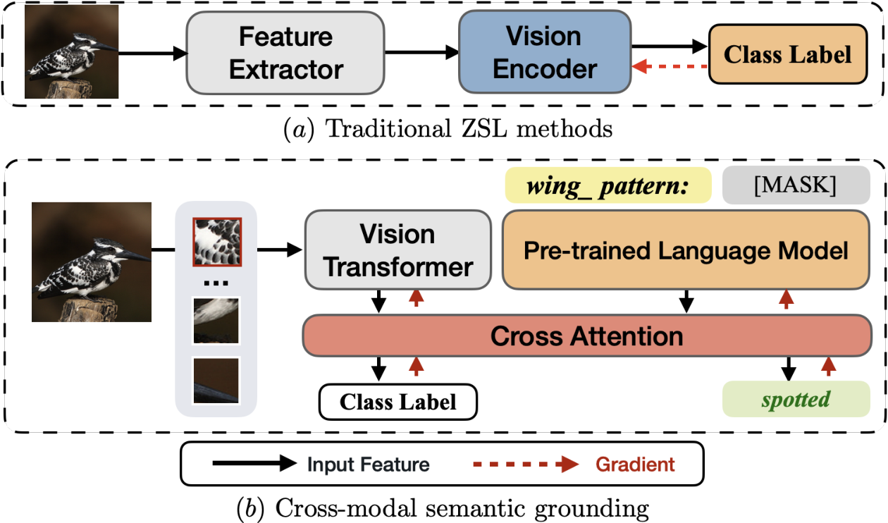
To address these issues, we propose a novel end-to-end ZSL framework named DUET (Cross-moDal Semantic GroUnding for ContrastivE Zero-shoT Learning). Unlike previous ZSL methods in Figure 2(a) that emphasize utilizing more external class knowledge, augmenting data, or developing better vision encoders, we focus on transferring knowledge from PLMs to vision transformer encoder in a self-supervised manner, as shown in Figure 2(b), which gives the model the ability for fine-grained semantic grounding (i.e., the ability for locating relevant visual characteristics in an image given a textual attribute).
Specifically, we utilize a prompt-based Feature-to-Sequence Transformation (FST) proxy to transform different types of attributes into a textual sequence, which makes our model compatible to multiple ZSL tasks with different side information. A Cross-modal Semantic Grounding (CSG) network is developed to leverage the semantics in a PLM via a multi-task learning procedure, where we employ two switchable learning objectives: basic ZSL classification and cross-modal mask reconstruction (CMR). Moreover, we propose an attribute-level contrastive learning (ACL) mechanism as shown in Figure 1(c), where distinctive classes are selected as positive references when they are associated with one common attribute (e.g., “spotted”) and those similar classes as negative references when they have mutually exclusive attributes (e.g., “striped”) toward the same aspect (e.g., “wing_pattern”) of the image. This mechanism enables the model to distinguish subtle attribute differences between closed images, and find out the overlapped features between different images. The contributions can be summarized as:
- •
To the best of our knowledge, DUET is the first to investigate PLMs for zero-shot image classification. It includes a novel end-to-end multi-modal learning paradigm.
- •
A cross-modal semantic grounding network is developed for effective knowledge transfer from the PLM to the vision transformer encoder. An attribute-level contrastive learning mechanism is proposed to address the attribute imbalance and co-occurrence issues, which further enhances the model’s ability for distinguishing fine-grained vision characteristics in both seen/unseen images. Extensive experiments have been done on standard ZSL benchmarks equipped with attributes and one ZSL benchmark equipped with a knowledge graph. The results have verified our DUET’s effectiveness and interpretation capability. Our code is available at github.com/zjukg/DUET.
2 Related Work
2.1 Zero-shot Image Classification
The core idea of zero-shot image classification is to transfer semantic knowledge from seen classes to unseen classes based on their semantic information (Chen et al. 2021a; Chen et al. 2021b).

Embedding-based ZSL methods (Frome et al. 2013) intend to build mapping functions toward the images and/or the classes, and whether a class is the label of a sample can be determined by matching their vectors in the same space using similarity metrics. However, the lack of visual samples for the unseen classes causes the bias problem and restrict their capabilities in transferring knowledge. To mitigate this issue, the Generative ZSL methods (Chen et al. 2021d; Chen et al. 2021c; Geng et al. 2021a) are introduced to use various generative models (e.g., VAEs and GANs ) for creating synthetic data based on semantic features (e.g., simple attribute values (Naeem et al. 2021), knowledge graphs (Pan et al. 2017; Geng et al. 2021a) or textual descriptions (Chen and Yeh 2021)). Those data augmentation strategies can compensate for the shortage of unseen classes and convert ZSL into a supervised classification task. However, they are all complex in structure (not end-to-end) and difficult to train (owing to instability) (Pourpanah et al. 2020). The lack of region-attribute supervision data also makes it difficult to accurately understand the corresponding relationship of different attribute-feature pairs during training. Recently, some Attention-based methods begin to explore the discriminative region features guided by attentive semantic information. Specifically, RGEN (Xie et al. 2020) devises the attention technique to construct a region graph for transferring knowledge among different classes. GEM-ZSL (Liu et al. 2021a) utilizes gaze embedding to improve the localization of discriminative attributes. MSDN (Chen et al. 2022b) incorporates mutually visual-attribute attention sub-net for semantic distillation, while TransZero (Chen et al. 2022a) further extends MSDN via improving the attention layers by transformers. However, they are still confused by the universal phenomena of the attribute imbalance and co-occurrence (Zhao et al. 2019; Wang et al. 2021a), as shown in Figure 1. Meanwhile, the scope and availability of the input knowledge limit the performance of these models on ZSL.
In contrast to these methods, we leverage the semantic knowledge in PLMs, and design a cross-modal semantic grounding network to encourage the model to separate those attributes from images. Furthermore, we develop an attribute-level contrastive learning mechanism to address the attribute imbalance and co-occurrence issues, which further enhances the model’s discrimination of different independent characteristics in a self-supervised manner.
3 Methodology
Let be the training set, where is an image with label attached, and be the unseen dataset, where and are disjoint. Each label corresponds to a class . Specifically, ZSL aims to recognize images of unseen classes () by transferring learned knowledge from seen classes () using their side information (e.g., attributes). In this study, we assume attributes annotated to classes are given, where each attribute is sometimes associated with a real or binary value for indicating its degree. All the attributes of a dataset are denoted as , and the attributes of a class is denoted as .
3.1 Feature-to-Sequence Transformation
This module unifies attributes of each class into a textual format. For ZSL datasets with binary format attributes, we assume is in the attribute set of class if . Specifically, we propose a prompt-based policy to semi-serialize these discrete attributes to accommodate the sequential inputs of PLMs, inspired by the structured tabular data pre-training (Yin et al. 2020). Concretely, we cluster fine-grained attributes to define class-specific prompt set (i.e., abstract attribute set) where . Then, given a class , we semi-serialize its attributes with prompt (name) put ahead of each , and take special symbol “” for prompt set separation. Taking the encoded attribute sentence for the class “Otter” in AWA2 (Xian et al. 2019) dataset as an example:
| (1) |
Obviously, compared to annotating large-scale fine-grained attributes for each image, it is easier to cluster limited attribute names. Since many ZSL datasets already have their incipient attribute divisions such as SUN (Patterson and Hays 2012), we just need to make little adjustments like removing the repeated prefixes (e.g., “has”) and revising some ambiguous . For knowledge-based ZSL (a.k.a. K-ZSL) datasets such as AWA2-KG in OntoZSL (Geng et al. 2021a), given a triple (, , ), e.g., (Zebra, hasPart, Four_legs), we simply take the relation as the prompt of attribute .
3.2 Cross-modal Semantic Grounding
This module enables the knowledge transfer from the PLM to the vision transformer encoder via attribute phrase masking and cross-modal mask reconstruction.
Attribute Phrase Masking (APM).
We apply an APM strategy to mask a complete attribute phrase at each step and then urge the model to recover it. We think discriminative attributes with low frequency within the attribute collection are more important. Therefore, we sample the target attribute to be masked via a linear weighted random sampling (LWRS) strategy: . Given a class , the probability for sampling attribute as the is:
| (2) |
where is an indicator function (i.e., it is 1 when , otherwise 0).
Since the scale of non-repetitive attribute sentence is normally much smaller than (i.e., ), we propose random attributes pruning (RAP) over the to remove part of the attributes (except ) toward a class within each training step. Specifically, we denote with hyperparameter as the pruning ratio. This will make the model to recover the attribute based on relevant visual information rather than trickily utilizing attribute co-occurrence. Thus, the masked attribute sentence constructed based on , denoted as , is the input of PLM encoder.
Cross-modal Mask Reconstruction (CMR).
We leverage the transformer architecture to encode both the visual features and textual attributes. Specifically, we split an image (in class ) into patches sequence and feed them into the vision transformer encoder with 1-D position embedding attached. Meawhile, a learnable embedding (marked with [CLS]) is prepended whose state at the output serves as the representation of the image. Subsequently, as shown in Figure 3, cross attention layers are stacked behind the parallel encoders for cross-modal information transfer. Each of them consists of one bi-directional cross-attention block, two self-attention blocks and two feed-forward blocks. A residual connection and layer normalization are added behind each block. The keys and values (Vaswani et al. 2017) from each modality are passed as the input to other modality’s multi-headed attention blocks. Let and be the output representation of image and the masked target attribute, respectively. The objective for CMR is
| (3) |
where represents the token sequence of target attribute in PLM’s vocabulary , Specifically, is the expressive degree score for attribute in class , which adaptively gives more weights to those highly confident attributes (i.e., conspicuous characteristics in a class). Moreover, we denote
| (4) |
where refers to the token embedding of .
Basic ZSL Classification.
Following (Chen et al. 2022a; Xu et al. 2020), we present the attribute regression loss to encourage DUET to accurately map the image representation into corresponding attribute embedding:
| (5) |
where is the class-level attribute vector for image . Meanwhile, we utilize the cross-entropy loss to enforce the image to have the highest compatibility score with its corresponding class semantic vector:
| (6) |
To further strengthen DUET’s discriminative ability towards different classes with limited samples, we define a class-level supervised contrastive loss:
| (7) |
where is the input sentence on language side. Specifically, let be the representation of positive image which has the same class label as , those features with distinct label inside the mini-batch make up a negative samples . We define as:
| (8) |
where is the temperature hyper-parameter. denotes the cosine similarity between and , where is a non-linear projection head (Chen et al. 2020).
Multi-task Learning.
As the core part of cross-modal semantic grounding (CSG), the multi-task learning procedure (Sener and Koltun 2018; Whitehead et al. 2021) forces the model to spread attribute information between the vision side and the language side via a task switching strategy. Namely, DUET conducts CMR at stage by accessing the visual patches and , and conducts simple image classification task at stage without seeing the textual attributes. Specifically, the input sequence at is fixed as the prompt template to mimic the single-modal testing phase:
| (9) |
Let , be the loss function of basic ZSL classification and CSG, respectively. At each step, we apply the objective (for ) with probability , or (for ) with probability :
| (10) | ||||
| (11) |
where we denote as the “ZSL loss”.
| Methods | CUB | SUN | AWA2 | ||||||||||
| CZSL | GZSL | CZSL | GZSL | CZSL | GZSL | ||||||||
| T1 | U | S | H | T1 | U | S | H | T1 | U | S | H | ||
| TF-VAEGAN (ECCV) (Narayan et al. 2020) | 64.9 | 52.8 | 64.7 | 58.1 | 66.0 | 45.6 | 40.7 | 43.0 | 72.2 | 59.8 | 75.1 | 66.6 | |
| Composer (NeurIPS) (Huynh and Elhamifar 2020a) | 69.4 | 56.4 | 63.8 | 59.9 | 62.6 | 55.1 | 22.0 | 31.4 | 71.5 | 62.1 | 77.3 | 68.8 | |
| CE-GZSL (CVPR) (Han et al. 2021) | 77.5 | 63.1 | 66.8 | 65.3 | 63.3 | 48.8 | 38.6 | 43.1 | 70.4 | 63.1 | 78.6 | 70.0 | |
| GCM-CF (CVPR) (Yue et al. 2021) | – | 61.0 | 59.7 | 60.3 | – | 47.9 | 37.8 | 42.2 | – | 60.4 | 75.1 | 67.0 | |
| FREE (ICCV) (Chen et al. 2021c) | – | 55.7 | 59.9 | 57.7 | – | 47.4 | 37.2 | 41.7 | – | 60.4 | 75.4 | 67.1 | |
| HSVA (NeurIPS) (Chen et al. 2021d) | 62.8 | 52.7 | 58.3 | 55.3 | 63.8 | 48.6 | 39.0 | 43.3 | – | 59.3 | 76.6 | 66.8 | |
| AGZSL (ICLR) (Chou, Lin, and Liu 2021) | 57.2 | 41.4 | 49.7 | 45.2 | 63.3 | 29.9 | 40.2 | 34.3 | 73.8 | 65.1 | 78.9 | 71.3 | |
| APN (NeurIPS) (Xu et al. 2020) | 72.0 | 65.3 | 69.3 | 67.2 | 61.6 | 41.9 | 34.0 | 37.6 | 68.4 | 57.1 | 72.4 | 63.9 | |
| DVBE (CVPR) (Min et al. 2020) | – | 53.2 | 60.2 | 56.5 | – | 45.0 | 37.2 | 40.7 | – | 63.6 | 70.8 | 67.0 | |
| DAZLE (CVPR) (Huynh and Elhamifar 2020b) | 66.0 | 56.7 | 59.6 | 58.1 | 59.4 | 52.3 | 24.3 | 33.2 | 67.9 | 60.3 | 75.7 | 67.1 | |
| RGEN (ECCV) (Xie et al. 2020) | 76.1 | 60.0 | 73.5 | 66.1 | 63.8 | 44.0 | 31.7 | 36.8 | 73.6 | 67.1 | 76.5 | 71.5 | |
| GEM-ZSL (CVPR) (Liu et al. 2021a) | 77.8 | 64.8 | 69.3 | 67.2 | 62.8 | 38.1 | 35.7 | 36.9 | 67.3 | 64.8 | 77.5 | 70.6 | |
| MSDN (CVPR) (Chen et al. 2022b) | 76.1 | 68.7 | 67.5 | 68.1 | 65.8 | 52.2 | 34.2 | 41.3 | 70.1 | 62.0 | 74.5 | 67.7 | |
| TransZero (AAAI) (Chen et al. 2022a) | 76.8 | 69.3 | 68.3 | 68.8 | 65.6 | 52.6 | 33.4 | 40.8 | 70.1 | 61.3 | 82.3 | 70.2 | |
| DUET (Ours) | 72.3 | 62.9 | 72.8 | 67.5 | 64.4 | 45.7 | 45.8 | 45.8 | 69.9 | 63.7 | 84.7 | 72.7 | |
3.3 Attribute-level Contrastive Learning
To further strengthen the model’s sensitivity on subtle visual differences against the attribute co-occurrences, we introduce an attribute-level contrastive learning (ACL) module with the adaptive loss function:
| (12) |
where follows the base formulation of Eq. (8), but there are main differences between and :
(i) Target Object and Stage. targets at the mean-pooling representation of on language side of stage , where the input sentence is . While targets at the feature () on vision side, which is applied at stage with a fixed prompt template (9) as the .
(ii) Sampling Strategy. For class-level , we simply pick those images, which share the same class label with original sample as positive, and then define the rest as in-batch negative. While for attribute-level , we design an attribute-based sampling strategy: Given a class and its target attribute , we assume as the negative attribute from seen class , and as the positive attribute from seen class . We claim the precondition as:
| (13) | |||
| (14) |
where is the original class-agnostic prompt set that belongs to, and , is the class-specific prompt set in class , . All , that satisfies this precondition make up the candidate class set and , respectively.
(iii) Sampling Probability. We employ a heuristic process to let the model select those whose are more inconsistent, and whose are more similar, compared with . Then, we non-repetitively choose instances (i.e. and ) from these classes, and encode them by DUET to get the final and . Note that and are not masked to accelerate the convergence.
Finally, we stack this pluggable ACL module into CSG:
| (15) |
Remark 1
Considering the example in Figure 1, we assume “Pied Kingfisher” as the original bird class () with target attribute “spotted” () in the prompt set “wing pattern” (). We are likely to sample “Chuck will’s widow” as the positive class which contains spotted wing pattern, but has a low class similarity (28.6% after normlization) compared with “Pied Kingfisher”. Besides, we prefer to sample “Black-and-white Warbler” as the negative class whose wing pattern is striped (not “spotted”) but the class characteristic is pretty closed (73.8%) to “Pied Kingfisher”.
3.4 Zero-Shot Prediction
After training DUET, we use the learned cosine metric space for zero-shot recognition. There are two evaluation settings: conventional ZSL (CZSL), which classifies the testing samples with candidate classes from ; generalized ZSL (GZSL), which extends the candidate classes to . Specifically, we take the prompt template together with an test image as the input. Following (Liu et al. 2021a; Chen et al. 2022b), we predict the label via:
| (16) |
where if is a seen class and 0 otherwise. is the calibration factor tuned on a held-out validation set, and corresponds to the CZSL/GZSL setting respectively.
4 Experiments
4.1 Datasets
We select three standard attribute equipped ZSL benchmarks AWA2 (Xian et al. 2019), CUB (Welinder et al. 2010), SUN (Patterson and Hays 2012) with their splits proposed in (Xian et al. 2019), as well as a knowledge graph equipped benchmark AWA2-KG which has the same split as AWA2 but includes semantic information about hierarchical classes and attributes, for evaluation. In AWA2-KG, we assume that the class has the attribute when the length of the shortest same-direction relation path between them in KG is , where is a hyperparameter. For example, given two triples (Zebra, hasPart, Four_legs) and (Four_legs, subClassOf, Leg), the attribute of class “Zebra” is “Four_leg” when 1 and “Leg” when 2. Since we observe that the attribute become more coarse-grained when they are far away from the class in KG, we simply define as .
Besides, there are also some other ZSL datasets like aPY (Farhadi et al. 2009) and AWA1 (Lampert, Nickisch, and Harmeling 2014). We do not evaluate on them since most of their unseen classes are leakage (Xian et al. 2019) in ImageNet-1K (Deng et al. 2009), which is a common image datasets for normal vision encoder pre-training.
4.2 Experimental Settings
Unlike previous ZSL studies which pre-extract the image features using a pre-trained CNN model e.g., ResNet (He et al. 2016), we take as input the raw images and apply vision transformer to interact with the PLM for knowledge transfer. For those coefficients in AWA2, we set to 0.01, to 0.05, to 1, to 0.01, to 0.5, to 0.4 and to 0.8. We report the class-averaged (macro) accuracy as the basic metric, following the current literature (Xu et al. 2020; Chen et al. 2022a).
4.3 Overall Results
Standard ZSL Datasets.
We compare our method with 14 representative or state-of-the-art (SOTA) methods proposed in recent three years. These baselines are divided into two categories: non-generative (Xu et al. 2020; Min et al. 2020; Huynh and Elhamifar 2020b; Xie et al. 2020; Liu et al. 2021a; Chen et al. 2022b; Chen et al. 2022a) and generative (Narayan et al. 2020; Huynh and Elhamifar 2020a; Han et al. 2021; Yue et al. 2021; Chen et al. 2021c; Chen et al. 2021d; Chou, Lin, and Liu 2021). All those non-generative methods are attention-based except for DVBE (Min et al. 2020).
SUN contains more than 700 scene classes but each class has only 10-20 images instances, where the attribute imbalance and co-occurrence problem are universal. We find that DUET achieves the best accuracy (45.8) on with a large margin (2.5) compared with those SOTA methods, and surpass MSDN by 4.5 on , which is the SOTA no-generative methods on SUN. On AWA2, DUET gains 1.2 improvements over the SOTA performance, and outperforms the transformer-based method TransZero on all the GZSL metrics. On CUB, DUET achieves competitive performance, surpassing all generative methods on , except for the attention-based methods TransZero and MSDN. We own this to the fact that the prompts in CUB are mostly region-related (e.g., ““breast_color” and “wing_color”), but DUET simply attaches the image patches with sequential 1-dimensional positional embedding as the input, making it hard to capture the fine-grained positional relationship. Instead, TransZero takes 2D center coordinates to construct learnable relative region geometric embeddings for feature augmentation, which gets accurate position representations and helps the model achieve good performance. Notably, when it does not use feature augmentation from relative geometry relationships, the on CUB dramatically decreases to 66.5 (Chen et al. 2022a).
It is worth mentioning that DUET also achieves great performance on seen classes () on all three datasets, outperforming all baselines on SUN and AWA2 by at least 5.1 and 2.4 respectively. This proves that DUET well preserves the predictive ability on seen classes in addressing unseen classes.
K-ZSL Dataset.
We evaluate on AWA2-KG (Geng et al. 2021a) to validate DUET’s flexibility on various ZSL attribute formats. Specifically, we pick the KG from (Geng et al. 2021b) as the knowledge resource, and compare with baselines including DeViSE (Frome et al. 2013), SYNC (Changpinyo et al. 2016), DGP (Kampffmeyer et al. 2019), LsrGAN† (Vyas, Venkateswara, and Panchanathan 2020). We abandon the real-value attributes for fairness, and follow (Geng et al. 2021a; Geng et al. 2022; Chen et al. 2021e) to take the KG embedding (Bordes et al. 2013) for entity class representation toward and . As shown in Figure 4(a), DUET achieves higher performance among all other methods. In particular, it achieves a 30.2 improvement on metric compared to the non-generative method DGP.

ViT-based DUET.
To get further insights into our model, we report the results of DUET with ViT-base (Dosovitskiy et al. 2021) as the vision encoder. Remarkably, since the released ViT-base is pre-trained on ImageNet-21K which may contain unseen objects, we only select 2 recent ViT-based ZSL methods, ViT-ZSL (Alamri and Dutta 2021) and IEAM-ZSL (Narayan et al. 2020), for comparison. As shown in Figure 4(b), DUET surpasses these two methods by a large margin (14.1 improvement on and 10.3 improvement on ) and also exceeds our SOTA performance () by 4.8. This supports that our DUET greatly ameliorates the ZSL ability where the original vision transformer is poor. We believe that the performance will be further improved by plugging in a better vision transformer encoder.
4.4 Ablation Studies
| Methods | H | |
| Only | 64.1 | 8.6 |
| [4pt/1pt] CSG | 66.5 | 6.2 |
| CSG | 61.7 | 11.0 |
| CSG | 64.9 | 7.8 |
| CSG | 66.9 | 5.8 |
| CSG | 67.4 | 5.3 |
| CSG | 68.4 | 4.3 |
| CSG | 69.2 | 3.5 |
| DUET (Full model) | 72.7 | - |
Component Analysis.
We evaluate various stripped-down versions of our proposed model to compare the () performance gain brought by different components on AWA2. Concretely, we observe that the performance drops sharply when (1) freezing the language transformer encoder . Although it can reduce the overall learnable parameters, it makes the model harder to understand the special relationship among prompts, textual attributes, and visual features. From the results of taking (2) only the prompt and (3) only concatenating attribute as sequence input without the prompt, we observe that employing our FST strategy for semi-serializing attributes indeed benefits our model with 4.3 improvement. We also exploit the influence of (4) randomly masking attributes, (5) not conducting attribute pruning, which leads to 2.3, 1.8 falls compared with (7) applying the full CSG, proofing the necessity of both sampling target attribute with adaptive weight and pruning part of the attribute. Besides, (6) abandoning class-level contrastive learning leads to 0.8 decrease. We own this to the fact that contrastive learning can help model learn better visual representations by narrowing the distance within a class in the latent space. Most importantly, our pluggable ACL module further boosts the performance by 3.5 based on CSG, which illustrates that both of these modules are beneficial.

Hyperparameter Analysis.
By comparing DUET’s performance in Figure 5, we conclude that: (i) The performance decrease when and are too large, since the weak signal from the self-supervised objectives (i.e., and ) will gradually overwhelm the signal from supervised class label (i.e., and ). (ii) When is close to 1 or 0, the protocol all drops below the baseline. This is because the model turns into a single-modal task without multi-task learning when . While when , DUET is forced to classify the image with attribute attached throughout the training, leading to model’s poor generalization capability at test stage. (iii) Furthermore, we try a wide range of , i.e. = {0, 0.2, 0.4, 0.5, 0.6, 0.7, 0.8}, and find that DUET works best when is set to 0.5.
4.5 Interpretation

To proofs DUET’s capability on disentangling image-specific semantic attributes, we feed an image into the well-trained DUET together with a crafted template: “:”, where each prompt name is involved with the [MASK] followed to recover attribute tokens Figure 6 shows the prediction results from the cases in SUN’s testing set. We observe that DUET can successfully retrieve most relevant attributes from the image given a concrete prompt, e.g., the “sport” function from a “basketball arena” and the “natural” light from an open-air “bus depot”.
Sometimes, there also exist unreasonable attribute pairs within a class in GT attribute sets. For example, (i) “oilrig” has both “still water” and “waves” as its attributes, which is contradictory; (ii) there is no “carpet” in this “living room” image, but it has high confidence. These situations occur when mutually exclusive attributes are independently contained in different images within the same class, since the class-level attribute values in SUN are collected by averaging the binary labels from annotators. In contrast, our DUET could achieve instance-level semantic grounding, correctly giving “waves” high score in this “oilrig”, and ignoreing “carpet” in this “living room”.
Besides, the scarce attribute “fire” is confidently predicted in the “oilrig” image, while in “living room”, the “flowers” are recovered without “leaves” bound together, which demonstrate the capability of DUET in addressing the attribute imbalance and attribute co-occurrence issues shown in Figure 1. Moreover, DUET can ground not only obvious visual attributes (e.g., “fire”) but also those abstract properties (e.g., “soothing” for “feeling” and “competting” for “technical function”), which shows its potential capability for knowledge inference.
5 Conclusion
In this paper, we propose an end-to-end ZSL framework named DUET to address the well known issues of attribute imbalance and co-occurrence in zero-shot image classification. We design a cross-modal semantic grounding network with a novel attribute-level contrastive learning mechanism to enhance the model’s discriminative ability towards novel classes, which could well address the issues of attribute imbalance and co-occurrence in zero-shot learning. With extensive ablation studies and the comparison with quite a few state-of-the-art methods on four ZSL benchmarks with real-valued and binary-valued attributes, we demonstrate the effectiveness of DUET as well as its support for interpretation.
Acknowledgement
We want to express gratitude to the anonymous reviewers for their hard work and kind comments. This work is partially funded by NSFCU19B2027/91846204, the EPSRC project ConCur (EP/V050869/1) and the Chang Jiang Scholars Program (J2019032).
References
- Alamri and Dutta (2021) Alamri, F.; and Dutta, A. 2021. Multi-Head Self-Attention via Vision Transformer for Zero-Shot Learning. CoRR, abs/2108.00045.
- Amosy et al. (2022) Amosy, O.; Volk, T.; Ben-David, E.; Reichart, R.; and Chechik, G. 2022. Text2Model: Model Induction for Zero-shot Generalization Using Task Descriptions. CoRR, abs/2210.15182.
- Bao, Dong, and Wei (2021) Bao, H.; Dong, L.; and Wei, F. 2021. BEiT: BERT Pre-Training of Image Transformers. CoRR, abs/2106.08254.
- Bordes et al. (2013) Bordes, A.; Usunier, N.; García-Durán, A.; Weston, J.; and Yakhnenko, O. 2013. Translating Embeddings for Modeling Multi-relational Data. In NIPS, 2787–2795.
- Changpinyo et al. (2016) Changpinyo, S.; Chao, W.-L.; Gong, B.; and Sha, F. 2016. Synthesized classifiers for zero-shot learning. In Proceedings of the IEEE conference on computer vision and pattern recognition, 5327–5336.
- Chen et al. (2021a) Chen, J.; Geng, Y.; Chen, Z.; Horrocks, I.; Pan, J. Z.; and Chen, H. 2021a. Knowledge-aware Zero-Shot Learning: Survey and Perspective. In IJCAI, 4366–4373. ijcai.org.
- Chen et al. (2021b) Chen, J.; Geng, Y.; Chen, Z.; Pan, J. Z.; He, Y.; Zhang, W.; Horrocks, I.; and Chen, H. 2021b. Low-resource Learning with Knowledge Graphs: A Comprehensive Survey. CoRR, abs/2112.10006.
- Chen et al. (2022a) Chen, S.; Hong, Z.; Liu, Y.; Xie, G.-S.; Sun, B.; Li, H.; Peng, Q.; Lu, K.; and You, X. 2022a. TransZero: Attribute-guided Transformer for Zero-Shot Learning. In AAAI.
- Chen et al. (2022b) Chen, S.; Hong, Z.; Xie, G.-S.; Yang, W.; Peng, Q.; Wang, K.; Zhao, J.; and You, X. 2022b. MSDN: Mutually Semantic Distillation Network for Zero-Shot Learning. In CVPR.
- Chen et al. (2021c) Chen, S.; Wang, W.; Xia, B.; Peng, Q.; You, X.; Zheng, F.; and Shao, L. 2021c. FREE: Feature Refinement for Generalized Zero-Shot Learning. In ICCV, 122–131.
- Chen et al. (2021d) Chen, S.; Xie, G.-S.; Peng, Q.; Liu, Y.; Sun, B.; Li, H.; You, X.; and Shao, L. 2021d. HSVA: Hierarchical Semantic-Visual Adaptation for Zero-Shot Learning. In 35th Conference on Neural Information Processing Systems (NeurIPS).
- Chen et al. (2020) Chen, T.; Kornblith, S.; Norouzi, M.; and Hinton, G. E. 2020. A Simple Framework for Contrastive Learning of Visual Representations. In ICML, volume 119, 1597–1607.
- Chen and Yeh (2021) Chen, Y.; and Yeh, M. 2021. Text-Enhanced Attribute-Based Attention for Generalized Zero-Shot Fine-Grained Image Classification. In ICMR, 447–450. ACM.
- Chen et al. (2021e) Chen, Z.; Chen, J.; Geng, Y.; Pan, J. Z.; Yuan, Z.; and Chen, H. 2021e. Zero-Shot Visual Question Answering Using Knowledge Graph. In ISWC, volume 12922 of Lecture Notes in Computer Science, 146–162.
- Chou, Lin, and Liu (2021) Chou, Y.; Lin, H.; and Liu, T. 2021. Adaptive and Generative Zero-Shot Learning. In ICLR.
- Cui et al. (2021) Cui, Y.; Che, W.; Liu, T.; Qin, B.; and Yang, Z. 2021. Pre-Training With Whole Word Masking for Chinese BERT. IEEE ACM Trans. Audio Speech Lang. Process., 29: 3504–3514.
- Deng et al. (2009) Deng, J.; Dong, W.; Socher, R.; Li, L.; Li, K.; and Fei-Fei, L. 2009. ImageNet: A large-scale hierarchical image database. In CVPR, 248–255.
- Devlin et al. (2019) Devlin, J.; Chang, M.; Lee, K.; and Toutanova, K. 2019. BERT: Pre-training of Deep Bidirectional Transformers for Language Understanding. In NAACL-HLT (1), 4171–4186.
- Dosovitskiy et al. (2021) Dosovitskiy, A.; Beyer, L.; Kolesnikov, A.; Weissenborn, D.; Zhai, X.; Unterthiner, T.; Dehghani, M.; Minderer, M.; Heigold, G.; Gelly, S.; Uszkoreit, J.; and Houlsby, N. 2021. An Image is Worth 16x16 Words: Transformers for Image Recognition at Scale. In ICLR.
- Du et al. (2022) Du, Y.; Shi, M.; Wei, F.; and Li, G. 2022. Boosting Zero-shot Learning via Contrastive Optimization of Attribute Representations. CoRR, abs/2207.03824.
- Farhadi et al. (2009) Farhadi, A.; Endres, I.; Hoiem, D.; and Forsyth, D. A. 2009. Describing objects by their attributes. In CVPR, 1778–1785.
- Frome et al. (2013) Frome, A.; Corrado, G. S.; Shlens, J.; Bengio, S.; Dean, J.; Ranzato, M.; and Mikolov, T. 2013. DeViSE: A Deep Visual-Semantic Embedding Model. In NIPS, 2121–2129.
- Geng et al. (2021a) Geng, Y.; Chen, J.; Chen, Z.; Pan, J. Z.; Ye, Z.; Yuan, Z.; Jia, Y.; and Chen, H. 2021a. OntoZSL: Ontology-enhanced Zero-shot Learning. In WWW, 3325–3336.
- Geng et al. (2021b) Geng, Y.; Chen, J.; Chen, Z.; Pan, J. Z.; Yuan, Z.; and Chen, H. 2021b. K-ZSL: resources for knowledge-driven zero-shot learning. arXiv preprint arXiv:2106.15047.
- Geng et al. (2022) Geng, Y.; Chen, J.; Zhang, W.; Xu, Y.; Chen, Z.; Pan, J. Z.; Huang, Y.; Xiong, F.; and Chen, H. 2022. Disentangled Ontology Embedding for Zero-shot Learning. CoRR, abs/2206.03739.
- Han et al. (2021) Han, Z.; Fu, Z.; Chen, S.; and Yang, J. 2021. Contrastive Embedding for Generalized Zero-Shot Learning. In CVPR, 2371–2381.
- He et al. (2021) He, K.; Chen, X.; Xie, S.; Li, Y.; Dollár, P.; and Girshick, R. B. 2021. Masked Autoencoders Are Scalable Vision Learners. CoRR, abs/2111.06377.
- He et al. (2016) He, K.; Zhang, X.; Ren, S.; and Sun, J. 2016. Deep Residual Learning for Image Recognition. In CVPR, 770–778. IEEE Computer Society.
- Huynh and Elhamifar (2020a) Huynh, D.; and Elhamifar, E. 2020a. Compositional Zero-Shot Learning via Fine-Grained Dense Feature Composition. In NeurIPS.
- Huynh and Elhamifar (2020b) Huynh, D.; and Elhamifar, E. 2020b. Fine-Grained Generalized Zero-Shot Learning via Dense Attribute-Based Attention. In CVPR, 4482–4492. Computer Vision Foundation / IEEE.
- Kampffmeyer et al. (2019) Kampffmeyer, M.; Chen, Y.; Liang, X.; Wang, H.; Zhang, Y.; and Xing, E. P. 2019. Rethinking Knowledge Graph Propagation for Zero-Shot Learning. In CVPR, 11487–11496.
- Lampert, Nickisch, and Harmeling (2014) Lampert, C. H.; Nickisch, H.; and Harmeling, S. 2014. Attribute-Based Classification for Zero-Shot Visual Object Categorization. IEEE Trans. Pattern Anal. Mach. Intell., 36(3): 453–465.
- Li et al. (2020) Li, X.; Yin, X.; Li, C.; Zhang, P.; Hu, X.; Zhang, L.; Wang, L.; Hu, H.; Dong, L.; Wei, F.; Choi, Y.; and Gao, J. 2020. Oscar: Object-Semantics Aligned Pre-training for Vision-Language Tasks. In ECCV (30), volume 12375 of Lecture Notes in Computer Science, 121–137. Springer.
- Liu et al. (2021a) Liu, Y.; Zhou, L.; Bai, X.; Huang, Y.; Gu, L.; Zhou, J.; and Harada, T. 2021a. Goal-Oriented Gaze Estimation for Zero-Shot Learning. In CVPR, 3794–3803.
- Liu et al. (2021b) Liu, Z.; Lin, Y.; Cao, Y.; Hu, H.; Wei, Y.; Zhang, Z.; Lin, S.; and Guo, B. 2021b. Swin Transformer: Hierarchical Vision Transformer using Shifted Windows. In ICCV, 9992–10002. IEEE.
- Lu et al. (2019) Lu, J.; Batra, D.; Parikh, D.; and Lee, S. 2019. ViLBERT: Pretraining Task-Agnostic Visiolinguistic Representations for Vision-and-Language Tasks. In NeurIPS, 13–23.
- Min et al. (2020) Min, S.; Yao, H.; Xie, H.; Wang, C.; Zha, Z.; and Zhang, Y. 2020. Domain-Aware Visual Bias Eliminating for Generalized Zero-Shot Learning. In CVPR, 12661–12670.
- Naeem et al. (2022) Naeem, M. F.; Xian, Y.; Gool, L. V.; and Tombari, F. 2022. I2DFormer: Learning Image to Document Attention for Zero-Shot Image Classification. CoRR, abs/2209.10304.
- Naeem et al. (2021) Naeem, M. F.; Xian, Y.; Tombari, F.; and Akata, Z. 2021. Learning Graph Embeddings for Compositional Zero-Shot Learning. In CVPR, 953–962.
- Narayan et al. (2020) Narayan, S.; Gupta, A.; Khan, F. S.; Snoek, C. G. M.; and Shao, L. 2020. Latent Embedding Feedback and Discriminative Features for Zero-Shot Classification. In ECCV (22), 479–495.
- Nawaz, Cavazza, and Bue (2022) Nawaz, S.; Cavazza, J.; and Bue, A. D. 2022. Semantically Grounded Visual Embeddings for Zero-Shot Learning. CoRR, abs/2201.00577.
- Pan et al. (2017) Pan, J. Z.; Vetere, G.; Gomez-Perez, J. M.; and Wu, H. 2017. Exploiting Linked Data and Knowledge Graphs in Large Organisations. Springer. ISBN 978-3-319-45652-2.
- Patterson and Hays (2012) Patterson, G.; and Hays, J. 2012. SUN attribute database: Discovering, annotating, and recognizing scene attributes. In CVPR, 2751–2758.
- Pourpanah et al. (2020) Pourpanah, F.; Abdar, M.; Luo, Y.; Zhou, X.; Wang, R.; Lim, C. P.; and Wang, X. 2020. A Review of Generalized Zero-Shot Learning Methods. CoRR, abs/2011.08641.
- Sener and Koltun (2018) Sener, O.; and Koltun, V. 2018. Multi-Task Learning as Multi-Objective Optimization. In NeurIPS, 525–536.
- Tan and Bansal (2019) Tan, H.; and Bansal, M. 2019. LXMERT: Learning Cross-Modality Encoder Representations from Transformers. In EMNLP/IJCNLP (1), 5099–5110.
- Touvron et al. (2021) Touvron, H.; Cord, M.; Douze, M.; Massa, F.; Sablayrolles, A.; and Jégou, H. 2021. Training data-efficient image transformers & distillation through attention. In ICML, volume 139 of Proceedings of Machine Learning Research, 10347–10357.
- Vaswani et al. (2017) Vaswani, A.; Shazeer, N.; Parmar, N.; Uszkoreit, J.; Jones, L.; Gomez, A. N.; Kaiser, L.; and Polosukhin, I. 2017. Attention is All you Need. In NIPS, 5998–6008.
- Vogel et al. (2022) Vogel, F.; Shvetsova, N.; Karlinsky, L.; and Kuehne, H. 2022. VL-Taboo: An Analysis of Attribute-based Zero-shot Capabilities of Vision-Language Models. CoRR, abs/2209.06103.
- Vyas, Venkateswara, and Panchanathan (2020) Vyas, M. R.; Venkateswara, H.; and Panchanathan, S. 2020. Leveraging seen and unseen semantic relationships for generative zero-shot learning. In European Conference on Computer Vision, 70–86. Springer.
- Wang et al. (2021a) Wang, L.; Huang, J.; Li, Y.; Xu, K.; Yang, Z.; and Yu, D. 2021a. Improving Weakly Supervised Visual Grounding by Contrastive Knowledge Distillation. In CVPR, 14090–14100. Computer Vision Foundation / IEEE.
- Wang et al. (2021b) Wang, W.; Xie, E.; Li, X.; Fan, D.; Song, K.; Liang, D.; Lu, T.; Luo, P.; and Shao, L. 2021b. Pyramid Vision Transformer: A Versatile Backbone for Dense Prediction without Convolutions. In ICCV, 548–558.
- Welinder et al. (2010) Welinder, P.; Branson, S.; Mita, T.; Wah, C.; Schroff, F.; Belongie, S.; and Perona, P. 2010. Caltech-UCSD birds 200.
- Whitehead et al. (2021) Whitehead, S.; Wu, H.; Ji, H.; Feris, R.; and Saenko, K. 2021. Separating Skills and Concepts for Novel Visual Question Answering. In CVPR, 5632–5641.
- Xian et al. (2019) Xian, Y.; Lampert, C. H.; Schiele, B.; and Akata, Z. 2019. Zero-Shot Learning - A Comprehensive Evaluation of the Good, the Bad and the Ugly. IEEE Trans. Pattern Anal. Mach. Intell., 41(9): 2251–2265.
- Xie et al. (2020) Xie, G.; Liu, L.; Zhu, F.; Zhao, F.; Zhang, Z.; Yao, Y.; Qin, J.; and Shao, L. 2020. Region Graph Embedding Network for Zero-Shot Learning. In ECCV (4), 562–580.
- Xu et al. (2020) Xu, W.; Xian, Y.; Wang, J.; Schiele, B.; and Akata, Z. 2020. Attribute Prototype Network for Zero-Shot Learning. In NeurIPS.
- Yin et al. (2020) Yin, P.; Neubig, G.; Yih, W.; and Riedel, S. 2020. TaBERT: Pretraining for Joint Understanding of Textual and Tabular Data. In ACL, 8413–8426.
- Yue et al. (2021) Yue, Z.; Wang, T.; Sun, Q.; Hua, X.; and Zhang, H. 2021. Counterfactual Zero-Shot and Open-Set Visual Recognition. In CVPR, 15404–15414.
- Zhang et al. (2021) Zhang, P.; Li, X.; Hu, X.; Yang, J.; Zhang, L.; Wang, L.; Choi, Y.; and Gao, J. 2021. VinVL: Revisiting Visual Representations in Vision-Language Models. In CVPR, 5579–5588.
- Zhao et al. (2019) Zhao, B.; Fu, Y.; Liang, R.; Wu, J.; Wang, Y.; and Wang, Y. 2019. A Large-Scale Attribute Dataset for Zero-Shot Learning. In CVPR Workshops, 398–407. Computer Vision Foundation / IEEE.
- Zhu et al. (2019) Zhu, Y.; Xie, J.; Liu, B.; and Elgammal, A. 2019. Learning Feature-to-Feature Translator by Alternating Back-Propagation for Generative Zero-Shot Learning. In ICCV, 9843–9853. IEEE.
Appendix A Appendix

A.1 Prompt Details
We cluster the attributes to define class-specific prompt sets for each ZSL dataset (task) as shown in Table 3.
For SUN dataset, (Patterson and Hays 2012) have already divided those scene attributes into four parts: “function”, “meterial”, “surface_property”, and “spatial_property”. As shown in Table 5, we further split them into 14 prompt sets requiring that the attributes within one set describe different characteristics toward the same aspect of the image. For example, we put “boating” and “driving” from the original “function” part into the more specific prompt set of “transportation fuction”. The details of the prompt sets of AWA2 (Xian et al. 2019) are shown in Table 6. The attribute categories of “color”, “pattern”, “shape” and “texture” are from ImageNet (Deng et al. 2009), and part pf the categories are from the LAD (Zhao et al. 2019).
While for CUB (Welinder et al. 2010) we simply extract the prefix from the attribute names as the prompt, e.g., we extract the “wing_color” prefix from the attribute“ has_wing_color:brown”, and make the “brown” as an attribute belongs to the “wing_color” prompt set. Particularly, different prompt sets may have intersections , e.g., the attribute “spotted” belongs to the prompt sets of “wing_pattern” and “head_pattern” simultaneously. More details are shown in Table 7.
A.2 Details for Experience in Sec. 4
| Dataset | # Pro. | # Att. |
|
| ||||
| CUB | 28 | 312 | 200 (150 / 50) | 7,057 / 4,731 | ||||
| SUN | 14 | 102 | 717 (645 / 72) | 10,320 / 4,020 | ||||
| AWA2 | 12 | 85 | 50 (40 / 10) | 23,527 / 13795 | ||||
| AWA2-KG | 17 | 120 | 50 (40 / 10) | 23,527 / 13795 |
Specifically, we use Swin-base (Liu et al. 2021b) as the vision transformer encoder for SUN, and DeiT-base (Touvron et al. 2021) for CUB, AWA2 and AWA2-KG. Both of their versions are pre-trained on ImageNet-1k. Let , , be the encoding function of vision transformer, PLM, and cross attention layer respectively. We apply Bert-base (Devlin et al. 2019) as the PLM encoder. We take the output embedding of [CLS] in and the whole output hidden state of as the input to . The cross attention layer number is set to 1. For each step in , when applying , we select 2 (i.e., select 2 images from each ) and 1 for each original image . For those coefficients, we set to 0.01, to 0.05, to 0.5, and to 0.05 for all datasets. Other dataset-specific hyperparameters are shown in Table 4. We use the AdamW optimizer (, ), and set the batch size to 50 and the learning rate to 3e-5. All the experiments are performed on three RTX 3090Ti GPUs. AWA2, which has the largest scale among our benchmarks which leads to least variance, is selected for all ablation studies.
| Dataset | ||||
| AWA2 | 1 | 0.01 | 0.8 | 0.4 |
| CUB | 5 | 0.001 | 0.6 | 0.4 |
| SUN | 1 | 0.01 | 0.5 | 0.5 |
| AWA2-KG | 0.5 | 0.01 | 0.7 | 0.4 |
A.3 Statistics for Attribute
Figure 7 shows part of the statistics about attribute co-occurrence and the imbalanced attribute distribution. Particularly, we define the frequency for those attributes as
| (17) |
where is 1 if is in , and 0 otherwise.
In order to measure the degree for attribute co-occurrence, we define the following metric:
| (18) |
For example, “flowers” appears with “leaves” 39 times, but “flowers” alone only appears 10 times, then , and . We observe that the distribution of different attributes varies greatly, and some unforeseen attribute pairs open appear together like (“cloth” “paper”) and (“clouds” “sand”).
A.4 Semantic Grounding and Visualization
Figure 8 visualizes the dense-attention maps on several test images in SUN. Compared with the BaseModel that only uses , our DUET can detect more accurate attribute regions that humans pay attention to. For example, for the “lock chamber” and “tunnel rail outdoor” images, we observe that the BaseModel fails to ground the “railroad” attribute, which is an infrequent attribute with the frequency of 2.09. Attribute imbalance issue may be the reason that BaseModel wrongly predicts these two images as “landing deck” and “fishpond”.
Moreover, since “waves”, “soil”, “asphalt” and “running water” always occur with “pavement”, “ocean”, “foliage” and “clouds” respectively, the BaseModel would fail to distinguish them in predicting the “flood”, “cavern indoor”, “palace”, and “creek” images which do not contain those latter accompanying attributes. In contrast, DUET better grounds those semantic attributes, leading to better overall performance. Lastly, our model also retains sensitivity for those key characteristics that are not obviously marked out in attribute set such as the teacups in “teashop” and the animals in “ranch”.
A.5 Sampling Strategy
We employ a heuristic process to let the model select those whose are more inconsistent, and whose are more similar, compared with . Concretely, we measure the class similarity via the Manhattan distance:
| (19) | ||||
| (20) |
and then set the class as positive or negative with a probability:
| (21) | ||||
| (22) |
where and .
A large number of experiments were conducted and we just selected the most optimal settings (highlight with bold):
- •
Regarding the strategy for choosing the target attributes, we have test (i) the random sampling; (ii) the linear weighted random sampling in Eq. (2); (ii) the non-linear weighted random sampling (simple based on squaring or softmax).
- •
- •
When it comes to the metric for class distance, we have tested (i) the Manhattan distance in Eq. (20); (ii) the Euclidean distance; (iii) the Cosine similarity.
A.6 Cross-Attention Layer in Sec. 3.2
Each cross-attention layer consists of one bi-directional cross-attention block, two self-attention blocks and two feed-forward blocks. A residual connection and layer normalization are added after each block. Specifically, let be the input features of the -th attention block ( is the output of ), the output state is computed by
| (23) | |||
| (24) | |||
| (25) |
where denotes the attention weights between elements and in the -th attention head, which is normalized by . Besides, , query (), key () and value () are learnable weights for -th head. Remarkably, given any , is in the set of when is the self-attention block. Contrarily, when is the cross-attention block, and should be originated from different encoders and have no intersection.

A.7 Related Work for PLMs
Stacked by multiple transformer (Vaswani et al. 2017) blocks, the pre-trained language models (PLMs) store an amount of knowledge via learning universal language representations on Internet corpora, which can prevent researchers from training a new model from scratch and benefits downstream NLP tasks. The Mask Language Model (MLMs) (Devlin et al. 2019; Cui et al. 2021; Yin et al. 2020) are pre-trained by recovering the masked semantic unit in a sentence. , which play important roles among all those PLMs. Specifically, the masked semantic unit in BERT (Devlin et al. 2019) is the word token, which is a sequence of characters that are grouped together to express some basic semantic information. Cui et al. (Cui et al. 2021) design a whole word masking (WWM) strategy, where the model always masks all tokens corresponding to a whole word at once. Yin et al. (Yin et al. 2020) propose TaBERT to linearize the tables which makes PLMs understand the structured data.
Inspired by the major success of transformer in NLP field, researchers have recently applied this architecture to CV fields (Wang et al. 2021b; Dosovitskiy et al. 2021; Touvron et al. 2021; He et al. 2021; Bao, Dong, and Wei 2021; Liu et al. 2021b). For example, the Vision Transformer (ViT) (Dosovitskiy et al. 2021) applies the sequences of image patches into pure transformer for image classification. Based on ViT, Touvron et al. (Touvron et al. 2021) further distill the knowledge from CNN-based model, while Swin Transformer (Liu et al. 2021b) computes attention within a local window via partitioning the window into multiple sub-patches. Previous Vision-Language Pre-training (VLP) models (Tan and Bansal 2019; Lu et al. 2019; Zhang et al. 2021; Li et al. 2020) also benefit many multi-modal tasks like visual question answering (VQA) and natural language visual reasoning (NLVR2). But normally, when a multi-modal network is applied to a single-modal task, its performance drops rapidly due to the missing modality. Not to mention performing on a zero-shot single-modal task.
In this paper, we design a novel architecture DUET, which is the first work to extend the PLM architecture to ZSL image classification task under a multi-modal paradigm. Instead of simply taking a fixed semantic embedding as the input (Nawaz, Cavazza, and Bue 2022), our model leverages the knowledge within a large scale PLM via a cross-modal semantic grounding method, as shown in Figure 2(b).
A.8 Vision Encoder Selection
Pre-trained on ImageNet-21k, the Vision Transformer (ViT) (Dosovitskiy et al. 2021) applies the sequences of image patches into a pure transformer for image classification, where a learnable embedding is applied to the sequence of embedding patches whose state serves as the image representation. Based on ViT, DeiT (Touvron et al. 2021) further distills knowledge from a CNN-based model and select a better hyperparameter combination, which trains on only the ImageNet-1k database but achieves comparable performance with ViT. Swin (Liu et al. 2021b) uses a multi-stage hierarchical architecture which computes attention within a local window via partitioning the window into multiple sub-patches. To capture interactions between different windows, window partitioning in Swin is gradually shifted along the hierarchy of the network to capture overlapping regions, which is suitable for capturing multi-scale attributes in SUN dataset. Thus, in this paper, we use Swin-base as the vision transformer encoder for SUN, and DeiT-base11 1 huggingface.co/facebook/deit-base-distilled-patch16-224 for CUB, AWA2, and AWA2-KG, which are all pre-trained on ImageNet-1k with a fixed patch size of pixels. Specifically, for a fair comparison, we utilize the official conversion script22 2 github.com/huggingface/transformers/blob/main/src/transformers/models/swin/convert˙swin˙timm˙to˙pytorch.py to make the timm-based33 3 github.com/rwightman/pytorch-image-models Swin model compatible with the huggingface44 4 huggingface.co/ transformer library.
Regarding the impact of backbone on the baseline’s performance, we note that simply changing the backbone to vision transformers may not lead to better results. Concretely, we replace the backbone of a non-generative model APN (Xu et al. 2020) and a generative model ABP (Zhu et al. 2019) from ResNet101 to our transformer backbones, and freeze (Fz) all layers for feature extraction (follow ABP) or jointly fine-tune part of the layers (follow APN) e.g. last 1(L1) or 2(L2) layers. All hyper-parameters remain unchanged for fairness. We find their performance all drop by [T1, H]%: (i) ABP: CUB: [10.9, 11.6]; AWA2: [9.9, 5.2]; SUN: [18.2, 14.4]. (ii) APN: CUB: Fz: [5.6, 6.8]; L1: [4.8, 5.3]; L2: [12.2, 14.8]; AWA2: Fz: [9.9, 8.4]; L1: [6.8, 4.5]; SUN: Fz: [3.8, 6.9]; L1: [4.1, 7.6].
A.9 Attribute prediction in Sec. 4.5
Specifically, we feed an image into the well-trained DUET together with a crafted template:
| (26) |
which contains all prompt names with a [MASK] token attached behind each of them. Those mask representations are used for attribute token prediction, where those tokens from the attributes in the prompt set constitute the predictable candidate tokens in PLM’s vocabulary. The token could be mapped into corresponding attributes (maybe more than one) for score accumulation. Then we select those attributes whose prediction score rank within the top-3 as the results, and normalize their scores by dividing each of them by their sum. We also normalize those confidence scores from the real-value attribute vectors in the original SUN dataset via global Min-Max normalization, i.e. . Then we choose those highly confident attributes, and denote them as the ground truth (GT) attributes.
A.10 Future Work
Regarding the ways to improve performance on CUB, we could consider involving 2D relative geometry relationships via adding relative position encoding. Meanwhile, due to the intra-class image differences (images of the sample bird class in CUB are different due to e.g., different image shooting angles and different bird ages), we think DUET could be further improved by e.g., applying instance-level feature similarity as an auxiliary sample filtering strategy on the basis of our attribute-level contrastive learning (ACL) method, or pre-grounding the object, to get higher quality positive / negative samples.
Moreover, we noticed that some recent works like CoAR-ZSL(Du et al. 2022), T2M-HN (Amosy et al. 2022), VL-Taboo (Vogel et al. 2022), and I2DFormer (Naeem et al. 2022) are proposed in the same period as ours to explore the potential of PLMs in ZSL community for zero-shot prediction/analysis. We insist that the trade-off between efficiency and performance is an important factor that needs to be considered in future works.
| prompt | attributes |
| transportation function | boating, driving, biking, climbing, swimming, digging |
| environment function | transporting, sunbathing, touring, hiking, camping, reading, bathing, eating, socializing, congregating, sports, playing, working |
| technical function | studying, teaching, research, diving, cleaning, queuing, competing, exercise, gaming, audience, farming, constructing, shopping, medical, using tools, business, praying |
| coarse meterial | fencing, railing, wire, asphalt, pavement, brick, concrete, metal, paper, wood, linoleum, plastic, stone, ocean |
| specific meterial | railroad, flowers, shingles, carpet, tiles, cloth, sand, marble, waves, running water, still water, ice, snow, smoke, fire |
| natural meterial | trees, grass, vegetation, shrubbery, foliage, leaves, soil, glass, clouds |
| light | natural light, direct sun/sunny, indoor light |
| surface | worn, glossy, matte, sterile, damp, dry, dirty, rusty |
| temperature | warm, cold |
| origin property | natural, man made |
| area | open, semi enclosed, enclosed |
| horizon | far away horizon, no horizon, rugged scene |
| direction | vertical, horizontal |
| feeling | symmetrical, cluttered, scary, soothing, stressful |
| prompt | attributes |
| color | black, white, blue, brown, gray, orange, red, yellow |
| pattern | patches, spots, stripes |
| texture | furry, hairless, tough skin |
| shape | big, small, bulbous, lean |
| has part | flippers, hands, hooves,pads, paws, long leg, long neck, tail, chew teeth, meat teeth, buck teeth, strain teeth, horns,claws, tusks,smelly, muscle |
| behaviour | flys, hops, swims, tunnels, walks |
| character | fast, slow, strong, weak, hibernate, inactive, nocturnal, active, agility |
| limb | bipedal, quadrupedal |
| diet | fish, meat, plankton, vegetation, insects |
| role | forager, grazer, hunter, scavenger, skimmer, stalker, domestic |
| habitat | new world, old world, arctic, coastal, desert, bush, plains, forest, fields, jungle, mountains, ocean, ground, water, tree, cave |
| habit | hibernate, fierce, timid, smart, group, solitary, nestspot |
| prompt | attributes |
| bill shape | curved, dagger, hooked, needle, hooked seabird, spatulate, all purpose, cone, specialized |
| wing color | blue, brown, rainbow, purple, auburn, grey, yellow, olive, green, pink, orange, black, white, red, buff |
| upperparts color | blue, brown, rainbow, purple, auburn, grey, yellow, olive, green, pink, orange, black, white, red, buff |
| underparts color | blue, brown, rainbow, purple, auburn, grey, yellow, olive, green, pink, orange, black, white, red, buff |
| breast pattern | solid,spotted,striped,multi colored |
| back color | blue, brown, rainbow, purple, auburn, grey, yellow, olive, green, pink, orange, black, white, red, buff |
| tail shape | forked, rounded, notched, fan shaped, pointed, squared |
| upper tail color | blue, brown, rainbow, purple, auburn, grey, yellow, olive, green, pink, orange, black, white, red, buff |
| head pattern | spotted, malar, crested, masked, unique, eyebrow, eyering, plain, eyeline, striped, capped |
| breast color | blue, brown, rainbow, purple, auburn, grey, yellow, olive, green, pink, orange, black, white, red, buff |
| throat color | blue, brown, rainbow, purple, auburn,grey, yellow, olive, green, pink, orange, black, white, red, buff |
| eye color | blue, brown, purple, auburn, grey, yellow, olive, green, pink, orange, black, white, red, buff |
| bill length | same as head, longer than head, shorter than head |
| forehead color | blue, brown, rainbow, purple, auburn, grey, yellow, olive, green, pink, orange, black, white, red, buff |
| under tail color | blue, brown, rainbow, purple, auburn, grey, yellow, olive, green, pink, orange, black, white, red, buff |
| nape color | blue, brown, rainbow, purple, auburn, grey, yellow, olive, green, pink, orange, black, white, red, buff |
| belly color | blue, brown, rainbow, purple, auburn, grey, yellow, olive, green, pink, orange, black, white, red, buff |
| wing shape | round, pointed, broad, conical, long |
| size | large, small, very large, medium, very small |
| shape | water upright perching, marsh chicken, long leg, duck, owl, gull, hummingbird, pigeon, tree clinging, hawk, sandpiper, upland ground, swallow, perching |
| back pattern | solid, spotted, striped, multi colored |
| tail pattern | solid, spotted, striped, multi colored |
| belly pattern | solid, spotted, striped, multi colored |
| primary color | blue, brown, rainbow, purple, auburn, grey, yellow, olive, green, pink, orange, black, white, red, buff |
| leg color | blue, brown, rainbow, purple, auburn, grey, yellow, olive, green, pink, orange, black, white, red, buff |
| bill color | blue, brown, rainbow, purple, auburn, grey, yellow, olive, green, pink, orange, black, white, red, buff |
| crown color | blue, brown, rainbow, purple, auburn, grey, yellow, olive, green, pink, orange, black, white, red, buff |
| wing pattern | solid, spotted, striped, multi colored |