Continuous-stage symplectic adapted exponential
methods for charged-particle dynamics with
arbitrary electromagnetic fields

Ting Li Address: T. Li: School of Mathematics and Statistics, Xi’an Jiaotong University, 710049 Xi’an, China Email address: litingmath@stu.xjtu.edu.cn and Bin Wang Address: Corresponding author. B. Wang: School of Mathematics and Statistics, Xi’an Jiaotong University, 710049 Xi’an, China Email address: wangbinmaths@xjtu.edu.cn

Abstract.

This paper is devoted to the numerical symplectic approximation of the charged-particle dynamics (CPD) with arbitrary electromagnetic fields. By utilizing continuous-stage methods and exponential integrators, a general class of symplectic methods is formulated for CPD under a homogeneous magnetic field. Based on the derived symplectic conditions, two practical symplectic methods up to order four are constructed where the error estimates show that the proposed second order scheme has a uniform accuracy in the position w.r.t. the strength of the magnetic field. Moreover, the symplectic methods are extended to CPD under non-homogeneous magnetic fields and three algorithms are formulated. Rigorous error estimates are investigated for the proposed methods and one method is proved to have a uniform accuracy in the position w.r.t. the strength of the magnetic field. Numerical experiments are provided for CPD under homogeneous and non-homogeneous magnetic fields, and the numerical results support the theoretical analysis and demonstrate the remarkable numerical behavior of our methods.

Keywords: Charged particle dynamics, Symplectic methods, Uniform error bounds, Exponential methods, Arbitrary electromagnetic fields.

AMS Subject Classification: 65P10, 65L05, 65L20, 78A35.

1. Introduction

In this article, we are concerned with numerical symplectic methods for the following charged-particle dynamics (CPD) (see [4, 19, 20, 21, 22, 24, 47])

\begin{array}[c]{ll}{\ddot{x}(t)=\dot{x}(t)\times\frac{B(x(t))}{\epsilon}+F(x(t))},\quad x(0)=x_{0},\quad\dot{x}(0)=\dot{x}_{0},\end{array}

(1.1)

where $x(t)\in\mathbb{R}^{3}$ represents the position of a particle moving in an electro-magnetic field, the magnetic field is described by $B(x)=\nabla_{x}\times A(x)$ with the vector potential $A(x)\in\mathbb{R}^{3}$ , $\epsilon\in(0,1]$ is a dimensionless parameter which is related to the strength of the magnetic field, and $F(x)$ is the nonlinear function of the form $F(x)=-\nabla U(x)$ with scalar potential $U(x)$ . The initial data $x_{0}$ and $\dot{x}_{0}$ are two given real-valued vectors independent of $\epsilon$ . In this paper, we denote the magnetic field $B(x)$ by $B(x)=\big(B_{1}(x),B_{2}(x),B_{3}(x)\big)^{\intercal}$ , where $B_{i}(x)\in\mathbb{R}$ for $i=1,2,3.$ Then it follows from the definition of the cross product that $\dot{x}\times B(x)=\tilde{B}(x)\dot{x},$ where the skew symmetric matrix $\tilde{B}(x)$ is given by $\tilde{B}(x)=\left(\begin{array}[]{ccc}0&B_{3}(x)&-B_{2}(x)\\ -B_{3}(x)&0&B_{1}(x)\\ B_{2}(x)&-B_{1}(x)&0\\ \end{array}\right).$ According to the conjugate momentum $p=v+\frac{A(x)}{\epsilon}=v-\frac{\tilde{B}(x)}{2\epsilon}x$ , the CPD (1.1) can be converted into a Hamiltonian system with the non-separable Hamiltonian

H(x,p)=\frac{1}{2}\left\|p+\frac{\tilde{B}(x)}{2\epsilon}x\right\|^{2}+U(x),

(1.2)

where $\left\|\cdot\right\|$ denotes the Euclidean norm. For the non-separable Hamiltonian (1.2), it is well known that its flow is symplectic ([23]), i.e., it preserves the differential 2-form $\sum\limits_{i=1}^{3}dx_{i}\wedge dp_{i}.$ In this work, we are devoted to the formulation and analysis of a novel kind of symplectic methods for CPD.

The CPD (1.1) arises in many applications such as plasma physics, astrophysics and magnetic fusion devices (see, e.g. [1, 4, 10, 35]) and a large variety of methods has been constructed and developed for numerical solutions of the system. For the normal magnetic field $\epsilon\approx 1$ , the Boris method proposed in [6] is popular due to its simplicity and good properties (cf. [20, 37]). Other classical schemes have also been proposed for CPD such as multistep methods [21, 46], splitting methods [30] and so on. In the recent few decades, structure-preserving methods for differential equations have received more and more attention ([3, 13, 18, 23, 32, 39, 41]). There are various structure-preserving methods which have been applied to CPD, including volume-preserving methods [26], energy-preserving integrators [8, 9, 31, 38], symmetric methods [21, 46] and symplectic methods [5, 27, 42, 44, 49, 50, 51]. It is noted that these structure-preserving methods are all designed for CPD with normal magnetic field $\epsilon\approx 1$ and no analysis has been given for the strong regime $0<\epsilon\ll 1$ . If one considers the methods mentioned above for CPD with $0<\epsilon\ll 1$ , the accuracy usually depends on $1/\epsilon^{j}$ for some $j>0$ and this makes the methods inefficient for small $\epsilon$ . Concerning the methods for CPD with strong regime $0<\epsilon\ll 1$ , to the best of my knowledge, most existed algorithms are devoted to the accuracy or long time near conservation [11, 12, 14, 15, 16, 19, 24, 25, 47]. Structure-preserving methods have not been considered and analysed for CPD with strong regime $0<\epsilon\ll 1$ .

From the point of Hamiltonian system, it is well known that symplecticity is a very important property, which has been investigated by many researchers ([13, 48]). Various symplectic methods have been derived such as symplectic Runge-Kutta methods [39], symplectic Runge-Kutta-Nyström methods [41], and continuous-stage symplectic methods [18, 34, 43]. However, as stated above, symplectic methods for CPD [27, 42, 44, 49, 50, 51] have only been designed for the system under normal magnetic fields and there is no numerical approximation or error analysis for strong magnetic fields.

In this article, we construct a new kind of symplectic methods for CPD with arbitrary electromagnetic fields and establish the rigorous error estimates. To formulate the methods, the ideas of exponential methods (see, e.g. [2, 17, 23, 28, 33, 45]) and continuous-stage methods will be employed. Moreover, the convergence of the obtained symplectic methods is rigorously researched, and the error estimates show that some proposed methods have a uniform accuracy in the position w.r.t. $\epsilon$ . This means that symplectic methods with uniform (w.r.t. $\epsilon$ ) error bounds are achieved in this paper, and performances superior to the standard symplectic methods are demonstrated on some examples.

In the analysis of symplecticity, we consider the differential 2-form for the methods. However, since the Hamiltonian is non-separable and the new methods are exponential type, some challenges and difficulties emerge in the achievement of symplectic conditions. To make the derivation go smoothly, we consider some transformations of the original system and the methods, and make well use of the antisymmetry of $\tilde{B}(x)$ . These transformations can keep the symplecticity of the methods, and thus symplectic methods can be formulated by deriving the symplectic conditions for the transformed methods. Concerning the convergence of the methods for CPD under nonhomogeneous magnetic fields, exponential variation-of-constants formula unfortunately does not hold and thence the local errors of exponential methods cannot be derived. In order to overcome this difficulty, we design a novel system called as linearized system and establish exponential variation-of-constants formula for it. The error between this linearized system and the original one is deduced and based on which, we manage to derive the convergence of the methods. Moreover, following this approach, a method with uniform second order error bound and very good long time energy conservation is obtained for CPD under maximal ordering magnetic fields [7, 24, 36]. For the system of this case, two filtered Boris algorithms were presented in [24] and they were proved to have uniform second order error bound but without long time behaviour. An energy-preserving method was constructed in [47] and uniform first order error estimate was established. Compared with the methods derived in [24, 47], the method proposed in this paper has both uniform second order accuracy and symplecticity, and is a brand-new method to CPD under maximal ordering magnetic fields.

The rest of this paper is organised as follows. In Section 2, for solving CPD with homogeneous magnetic field, we propose the scheme of continuous-stage adapted exponential methods and derive its symplectic conditions. Then two practical symplectic methods up to order four are presented in Section 3 and their properties including convergence and implementations are also studied there. At the end of Section 3, one numerical experiment is provided and the results show the favorable behaviour of the new methods in comparison with the Boris method and two symplectic Runge-Kutta methods. Moreover, the extension and application of the proposed symplectic methods to CPD with non-homogeneous magnetic fields are discussed in Section 4. Three practical methods as well as their error estimates are proposed and two numerical tests are given to demonstrate that they are sharp. Section 5 is devoted to the conclusions of this paper.

2. Adapted exponential methods and symplectic conditions

In this section, we shall propose the novel methods for (1.1) in a homogeneous magnetic field $B=\big(B_{1},B_{2},B_{3}\big)^{\intercal}$ and analyse their symplectic conditions. We start by the variation-of-constants formula of the CPD (1.1) which reads (see [24])

	$\displaystyle x(t_{n}+h)$	$\displaystyle=x(t_{n})+h\varphi_{1}(hM)v(t_{n})+h^{2}\int_{0}^{1}(1-\tau)\varphi_{1}((1-\tau)hM)F(x(t_{n}+h\tau))d\tau,$		(2.1)
	$\displaystyle v(t_{n}+h)$	$\displaystyle=\varphi_{0}(hM)v(t_{n})+h\int_{0}^{1}\varphi_{0}((1-\tau)hM)F(x(t_{n}+h\tau))d\tau,$		(2.1)

for any step size $h\geq 0$ and $t_{n}=nh$ , where $v(t):=\dot{x}(t)$ , $M=\frac{\tilde{B}}{\epsilon}$ and the $\varphi$ -functions are defined by (see [29])

\varphi_{0}(z)=e^{z},\ \ \varphi_{k}(z)=\int_{0}^{1}e^{(1-\sigma)z}\frac{\sigma^{k-1}}{(k-1)!}d\sigma,\ \ k=1,2,\ldots.

To derive the novel methods, we consider the variation-of-constants formula (2.1) and utilize the idea of continuous-stage methods, which leads to the following definition.

Definition 2.1.

(Adapted exponential methods) By denoting the numerical approximation $x_{n}\approx x(t_{n}),\,v_{n}\approx v(t_{n})$ and choosing $v_{0}=\dot{x}_{0}$ , a continuous-stage adapted exponential method for solving (1.1) is defined as

	$\displaystyle$	$\displaystyle X_{\tau}=x_{n}+\tau h\varphi_{1}(\tau hM)v_{n}+h^{2}\int_{0}^{1}{\alpha}_{\tau\sigma}(hM)F(X_{\sigma})d\sigma,$		(2.2)
		$\displaystyle x_{n+1}=x_{n}+h\varphi_{1}(hM)v_{n}+h^{2}\int_{0}^{1}\beta_{\tau}(hM)F(X_{\tau})d\tau,\ \ v_{n+1}=\varphi_{0}(hM)v_{n}+h\int_{0}^{1}\gamma_{\tau}(hM)F(X_{\tau})d\tau,$		(2.2)

where $h$ is the step size, $X_{\tau}$ is a function about $\tau$ , and the coefficients ${\alpha}_{\tau\sigma}(hM)$ , $\beta_{\tau}(hM)$ and $\gamma_{\tau}(hM)$ are functions depending on $hM$ . For the method adapted to the Hamiltonian system (1.2), we consider the continuous-stage adapted exponential method (2.2) as well as a momentum calculation

p_{n+1}=v_{n+1}-\frac{\tilde{B}}{2\epsilon}x_{n+1}.

In what follows, we derive the symplectic conditions of the method given in Definition 2.1. When applied to the non-separable Hamiltonian (1.2), the method is called as symplectic if it preserves the symplecticity exactly, i.e. ([23]),

\sum\limits_{J=1}^{3}dx_{n+1}^{J}\wedge dp_{n+1}^{J}=\sum_{J=1}^{3}dx_{n}^{J}\wedge dp_{n}^{J},

where the superscript $(\cdot)^{J}$ denotes the $J$ th component of a vector. To prove this statement, we first make some transformations of the system (1.1) and of the method (2.2). Since $\tilde{B}$ is a skew-symmetric matrix, it can be expressed as $\tilde{B}=K\Omega K^{\textup{H}},$ where $K$ is a unitary matrix and $\Omega=\textmd{diag}(-{\left\|B\right\|}\mathrm{i},0,{\left\|B\right\|}\mathrm{i})$ . Now we denote the new variables as

\tilde{x}(t)=K^{\textup{H}}x(t),\quad\tilde{v}(t)=K^{\textup{H}}v(t).

(2.3)

Then the system (1.1) becomes

\begin{array}[c]{ll}\frac{d}{dt}\left(\begin{array}[]{c}\tilde{x}\\ \tilde{v}\\ \end{array}\right)=\left(\begin{array}[]{cc}0&I\\ 0&\tilde{\Lambda}\mathrm{i}\\ \end{array}\right)\left(\begin{array}[]{c}\tilde{x}\\ \tilde{v}\\ \end{array}\right)+\left(\begin{array}[]{c}0\\ \tilde{F}(\tilde{x})\\ \end{array}\right),\quad\left(\begin{array}[]{c}\tilde{x}_{0}\\ \tilde{v}_{0}\\ \end{array}\right)=\left(\begin{array}[]{c}K^{\textup{H}}x_{0}\\ K^{\textup{H}}\dot{x}_{0}\\ \end{array}\right),\end{array}

where $\tilde{\Lambda}=\textmd{diag}(-\tilde{\zeta},0,\tilde{\zeta})$ with $\tilde{\zeta}=\frac{{\left\|B\right\|}}{\epsilon}$ and $\tilde{F}(\tilde{x})=K^{\textup{H}}F(K\tilde{x})=-\nabla_{\tilde{x}}U(K\tilde{x})$ .

It is noted that the vector $\tilde{x}$ is denoted by $\tilde{x}=(\tilde{x}^{1},\tilde{x}^{2},\tilde{x}^{3})^{\intercal}$ and all the vectors in $\mathbb{R}^{3}$ or $\mathbb{C}^{3}$ use the same notation in this paper. For the variables (2.3) and the property of $K$ , we observe that $\tilde{x}^{1}=\bar{\tilde{x}}^{3}$ , $\tilde{v}^{1}=\bar{\tilde{v}}^{3}$ , and $\tilde{x}^{2}$ , $\tilde{v}^{2}\in\mathbb{R}$ . We shall denote $\bar{\tilde{x}}^{3}$ as the conjugate of $\tilde{x}^{3}$ and the same expression is applied to other functions. In the light of (2.3), the corresponding Hamiltonian system (1.2) is given by

\begin{array}[c]{ll}{\dot{\tilde{x}}}=\nabla_{\tilde{p}}\tilde{H}(\tilde{x},\tilde{p})=\tilde{p}+\frac{1}{2}\tilde{\Lambda}\mathrm{i}\tilde{x},\ \ \ \ {\dot{\tilde{p}}}=-\nabla_{\tilde{x}}\tilde{H}(\tilde{x},\tilde{p})=-\frac{1}{2}\big(\tilde{\Lambda}\mathrm{i}\big)^{\textup{H}}\big(\tilde{p}+\frac{1}{2}\tilde{\Lambda}\mathrm{i}\tilde{x}\big)-\nabla_{\tilde{x}}\tilde{U}(K\tilde{x}),\end{array}

(2.4)

with $\tilde{H}(\tilde{x},\tilde{p})=\frac{1}{2}\left\|\tilde{p}+\frac{1}{2}\tilde{\Lambda}\mathrm{i}\tilde{x}\right\|^{2}+\tilde{U}(K\tilde{x}).$ For this transformed Hamiltonian system, the method (2.2) takes the following transformed form

		$\displaystyle\tilde{X}_{\tau}=\tilde{x}_{n}+h\tau\varphi_{1}\big(\tau W\big)\tilde{v}_{n}+h^{2}\int_{0}^{1}{\alpha}_{\tau\sigma}\big(W\big)\tilde{F}\big(\tilde{X}_{\sigma}\big)d\sigma,$		(2.5)
		$\displaystyle\tilde{x}_{n+1}=\tilde{x}_{n}+h\varphi_{1}\big(W\big)\tilde{v}_{n}+h^{2}\int_{0}^{1}\beta_{\tau}\big(W\big)\tilde{F}\big(\tilde{X}_{\tau}\big)d\tau,$
		$\displaystyle\tilde{v}_{n+1}=\varphi_{0}\big(W\big)\tilde{v}_{n}+h\int_{0}^{1}\gamma_{\tau}\big(W\big)\tilde{F}\big(\tilde{X}_{\tau}\big)d\tau,\ \ \tilde{p}_{n+1}=\tilde{v}_{n+1}-\frac{1}{2}\tilde{\Lambda}\mathrm{i}\tilde{x}_{n+1},$

where $W=h\tilde{\Lambda}\mathrm{i}$ .

Now we present symplectic conditions of the transformed method (2.5) and then get the symplecticity of the method given in Definition 2.1.

Theorem 2.2.

(Symplecticity) (a) For solving the transformed Hamiltonian system (2.4), the map $(\tilde{x}_{n},\tilde{p}_{n})\rightarrow(\tilde{x}_{n+1},\tilde{p}_{n+1})$ determined by the transformed method (2.5) is symplectic if the coefficients satisfy

$\displaystyle(i)$	$\displaystyle\gamma_{\tau}(W)-W\beta_{\tau}(W)=d_{\tau}I,\ \ d_{\tau}\in\mathbb{C},$	(2.6)
$\displaystyle(ii)$	$\displaystyle\gamma_{\tau}(W)(\bar{\varphi}_{1}(W)-\tau\bar{\varphi}_{1}(\tau W))=\beta_{\tau}(W)(e^{-W}+W\bar{\varphi}_{1}(W)-\tau W\bar{\varphi}_{1}(\tau W)),$
$\displaystyle(iii)$	$\displaystyle\bar{\beta}_{\sigma}(W)\gamma_{\tau}(W)-W\bar{\beta}_{\sigma}(W)\beta_{\tau}(W)/2-\bar{{\alpha}}_{\tau\sigma}(W)(\gamma_{\tau}(W)-W\beta_{\tau}(W))$
	$\displaystyle=\beta_{\tau}(W)\bar{\gamma}_{\sigma}(W)+W\beta_{\tau}(W)\bar{\beta}_{\sigma}(W)/2-{\alpha}_{\sigma\tau}(W)(\bar{\gamma}_{\sigma}(W)+W\bar{\beta}_{\sigma}(W)).$

(b) If the transformed method (2.5) is symplectic, the map $(x_{n},p_{n})\rightarrow(x_{n+1},p_{n+1})$ determined by Definition 2.1 is symplectic for solving the Hamiltonian system (1.2).

Proof.

We first prove the second statement (b). By the notation of differential 2-form and with the help of $K$ , we have

		$\displaystyle\sum\limits_{J=1}^{3}dx_{n+1}^{J}\wedge dp_{n+1}^{J}=\sum\limits_{J=1}^{3}d\bar{x}_{n+1}^{J}\wedge dp_{n+1}^{J}=\sum\limits_{J=1}^{3}d\big(\bar{K}\bar{\tilde{x}}_{n+1}\big)^{J}\wedge d\big(K\tilde{p}_{n+1}\big)^{J}$
	$\displaystyle=$	$\displaystyle\sum\limits_{J=1}^{3}\bigg({d}\sum\limits_{i=1}^{3}\big(\bar{K}_{Ji}\bar{\tilde{x}}_{n+1}^{i}\big)\bigg)\wedge\bigg({d}\sum\limits_{\iota=1}^{3}\big(K_{J\iota}\tilde{p}_{n+1}^{\iota}\big)\bigg)=\sum\limits_{J=1}^{3}\bigg(\sum\limits_{i=1}^{3}\big(\bar{K}_{Ji}{d}\bar{\tilde{x}}_{n+1}^{i}\big)\bigg)\wedge\bigg(\sum\limits_{\iota=1}^{3}\big(K_{J\iota}{d}\tilde{p}_{n+1}^{\iota}\big)\bigg)$
	$\displaystyle=$	$\displaystyle\sum\limits_{J=1}^{3}\sum\limits_{i=1}^{3}\sum\limits_{\iota=1}^{3}\bar{K}_{Ji}K_{J\iota}\big({d}\bar{\tilde{x}}_{n+1}^{i}\wedge{d}\tilde{p}_{n+1}^{\iota}\big)=\sum\limits_{i=1}^{3}{d}\bar{\tilde{x}}_{n+1}^{i}\wedge{d}\tilde{p}_{n+1}^{i}=\sum\limits_{J=1}^{3}{d}\bar{\tilde{x}}_{n+1}^{J}\wedge{d}\tilde{p}_{n+1}^{J}.$

Likewise, one gets $\sum\limits_{J=1}^{3}dx_{n}^{J}\wedge dp_{n}^{J}=\sum\limits_{J=1}^{3}{d}\bar{\tilde{x}}_{n}^{J}\wedge{d}\tilde{p}_{n}^{J}.$ Hence the second statement is hold.

For the first statement (a), we need to prove $\sum\limits_{J=1}^{3}{d}\bar{\tilde{x}}_{n+1}^{J}\wedge{d}\tilde{p}_{n+1}^{J}=\sum\limits_{J=1}^{3}{d}\bar{\tilde{x}}_{n}^{J}\wedge{d}\tilde{p}_{n}^{J},$ i.e.,

\displaystyle\sum\limits_{J=1}^{3}{d}\bar{\tilde{x}}_{n+1}^{J}\wedge{d}\tilde{v}_{n+1}^{J}-\frac{1}{2}\sum\limits_{J=1}^{3}{d}\bar{\tilde{x}}_{n+1}^{J}\wedge{d}\big(\tilde{\Lambda}^{J}\mathrm{i}\tilde{x}_{n+1}^{J}\big)=\sum\limits_{J=1}^{3}{d}\bar{\tilde{x}}_{n}^{J}\wedge{d}\tilde{v}_{n}^{J}-\frac{1}{2}\sum\limits_{J=1}^{3}{d}\bar{\tilde{x}}_{n}^{J}\wedge{d}\big(\tilde{\Lambda}^{J}\mathrm{i}\tilde{x}_{n}^{J}\big).

(2.7)

(I) Computation of the left hand side of (2.7). It is noted that $\overline{{d}\bar{\tilde{x}}_{n}^{J}\wedge{d}\tilde{v}_{n}^{J}}={d}\tilde{x}_{n}^{J}\wedge{d}\bar{\tilde{v}}_{n}^{J}$ and ${d}\bar{\tilde{x}}_{n}^{J}\wedge{d}\tilde{x}_{n}^{J}\in\mathrm{i}\mathbb{R}$ , and denote the method by

		$\displaystyle\tilde{X}^{J}_{\tau}=\tilde{x}^{J}_{n}+h\tau\varphi_{1}\big(\tau{W}^{J}\big)\tilde{v}^{J}_{n}+h^{2}\int_{0}^{1}{\alpha}_{\tau\sigma}\big({W}^{J}\big)\tilde{F}^{J}_{\sigma}d\sigma,$		(2.8)
		$\displaystyle\tilde{x}^{J}_{n+1}=\tilde{x}^{J}_{n}+h\varphi_{1}({W}^{J})\tilde{v}^{J}_{n}+h^{2}\int_{0}^{1}\beta_{\tau}\big({W}^{J}\big)\tilde{F}^{J}_{\tau}d\tau,\ \ \tilde{v}^{J}_{n+1}=e^{{W}^{J}}\tilde{v}^{J}_{n}+h\int_{0}^{1}\gamma_{\tau}\big({W}^{J}\big)\tilde{F}^{J}_{\tau}d\tau,$		(2.8)

where the superscript $(\cdot)^{J}$ is the $J$ th component of a vector or a matrix and $\tilde{F}^{J}_{\tau}$ is the $J$ th component of $\tilde{F}\big(\tilde{X}_{\tau}\big)$ . Based on the above expression, in what follows we calculate the left hand side of (2.7).

Inserting the scheme of (2.8) into (2.7), it arrives that

$\displaystyle$	$\displaystyle\sum\limits_{J=1}^{3}\bigg(d\bar{\tilde{x}}_{n+1}^{J}\wedge d\tilde{v}_{n+1}^{J}-\frac{1}{2}d\bar{\tilde{x}}_{n+1}^{J}\wedge d\big(\tilde{\Lambda}^{J}\mathrm{i}\tilde{x}_{n+1}^{J}\big)\bigg)=\sum\limits_{J=1}^{3}\bigg(e^{{W}^{J}}d\bar{\tilde{x}}_{n}^{J}\wedge d\tilde{v}_{n}^{J}+h\int_{0}^{1}\Big(\gamma_{\tau}\big({W}^{J}\big)d\bar{\tilde{x}}_{n}^{J}\wedge d\tilde{F}_{\tau}^{J}\Big)d\tau$	(2.9)
	$\displaystyle+he^{{W}^{J}}\bar{\varphi}_{1}\big({W}^{J}\big)d\bar{\tilde{v}}_{n}^{J}\wedge d\tilde{v}_{n}^{J}+h^{2}\int_{0}^{1}\Big(\bar{\varphi}_{1}\big({W}^{J}\big)\gamma_{\tau}\big({W}^{J}\big)d\bar{\tilde{v}}_{n}^{J}\wedge d\tilde{F}_{\tau}^{J}\Big)d\tau+h^{2}e^{{W}^{J}}\int_{0}^{1}\Big(\bar{\beta}_{\tau}\big({W}^{J}\big)d\bar{\tilde{F}}_{\tau}^{J}\wedge d\tilde{v}_{n}^{J}\Big)d\tau$
	$\displaystyle+h^{3}\int_{0}^{1}\int_{0}^{1}\Big(\bar{\beta}_{\tau}\big({W}^{J}\big)\gamma_{\sigma}\big({W}^{J}\big)d\bar{\tilde{F}}_{\tau}^{J}\wedge d\tilde{F}_{\sigma}^{J}\Big)d\tau d\sigma-\frac{1}{2}d\bar{\tilde{x}}_{n}^{J}\wedge d\big(\tilde{\Lambda}^{J}\mathrm{i}\tilde{x}_{n}^{J}\big)-\frac{1}{2}{W}^{J}\varphi_{1}\big({W}^{J}\big)d\bar{\tilde{x}}_{n}^{J}\wedge d\tilde{v}_{n}^{J}$
	$\displaystyle-\frac{1}{2}h{W}^{J}\int_{0}^{1}\Big(\beta_{\tau}\big({W}^{J}\big)d\bar{\tilde{x}}_{n}^{J}\wedge d\tilde{F}_{\tau}^{J}\Big)d\tau-\frac{1}{2}{W}^{J}\bar{\varphi}_{1}\big({W}^{J}\big)d\bar{\tilde{v}}_{n}^{J}\wedge d\tilde{x}_{n}^{J}-\frac{1}{2}h{W}^{J}\bar{\varphi}_{1}\big({W}^{J}\big)\varphi_{1}\big({W}^{J}\big)d\bar{\tilde{v}}_{n}^{J}\wedge d\tilde{v}_{n}^{J}$
	$\displaystyle-\frac{1}{2}h^{2}{W}^{J}\varphi_{1}\big({W}^{J}\big)\int_{0}^{1}\Big(\bar{\beta}_{\tau}\big({W}^{J}\big)d\bar{\tilde{F}}_{\tau}^{J}\wedge d\tilde{v}_{n}^{J}\Big)d\tau-\frac{1}{2}h^{3}{W}^{J}\int_{0}^{1}\int_{0}^{1}\Big(\bar{\beta}_{\tau}\big({W}^{J}\big)\beta_{\sigma}\big({W}^{J}\big)d\bar{\tilde{F}}_{\tau}^{J}\wedge d\tilde{F}_{\sigma}^{J}\Big)d\tau d\sigma$
	$\displaystyle-\frac{1}{2}h^{2}{W}^{J}\bar{\varphi}_{1}\big({W}^{J}\big)\int_{0}^{1}\Big(\beta_{\tau}\big({W}^{J}\big)d\bar{\tilde{v}}_{n}^{J}\wedge d\tilde{F}_{\tau}^{J}\Big)d\tau-\frac{1}{2}h{W}^{J}\int_{0}^{1}\Big(\bar{\beta}_{\tau}\big({W}^{J}\big)d\bar{\tilde{F}}_{\tau}^{J}\wedge d\tilde{x}_{n}^{J}\Big)d\tau\bigg).$

Considering the properties of coefficient functions and exterior product, we obtain

		$\displaystyle-\sum\limits_{J=1}^{3}\frac{1}{2}h{W}^{J}\bar{\varphi}_{1}\big({W}^{J}\big)d\bar{\tilde{v}}_{n}^{J}\wedge d\tilde{x}_{n}^{J}=-\sum\limits_{J=1}^{3}\frac{1}{2}h{W}^{J}\varphi_{1}\big({W}^{J}\big)d\bar{\tilde{x}}_{n}^{J}\wedge d\tilde{v}_{n}^{J},$
		$\displaystyle-\sum\limits_{J=1}^{3}\frac{1}{2}h{W}^{J}\int_{0}^{1}\Big(\bar{\beta}_{\tau}\big({W}^{J}\big)d\bar{\tilde{F}}_{\tau}^{J}\wedge d\tilde{x}_{n}^{J}\Big)d\tau=-\sum\limits_{J=1}^{3}\frac{1}{2}h{W}^{J}\int_{0}^{1}\Big(\beta_{\tau}\big({W}^{J}\big)d\bar{\tilde{x}}_{n}^{J}\wedge d\tilde{F}_{\tau}^{J}\Big)d\tau,$
		$\displaystyle-\sum\limits_{J=1}^{3}h^{2}\int_{0}^{1}\Big(\bar{\beta}_{\tau}\big({W}^{J}\big)e^{{W}^{J}}d\bar{\tilde{F}}_{\tau}^{J}\wedge d\tilde{v}_{n}^{J}\Big)d\tau=\sum\limits_{J=1}^{3}h^{2}\int_{0}^{1}\Big(\beta_{\tau}\big({W}^{J}\big)e^{-{W}^{J}}d\bar{\tilde{v}}_{n}^{J}\wedge d\tilde{F}_{\tau}^{J}\Big)d\tau,$
		$\displaystyle-\sum\limits_{J=1}^{3}\frac{1}{2}h^{2}{W}^{J}\varphi_{1}\big({W}^{J}\big)\int_{0}^{1}\Big(\bar{\beta}_{\tau}\big({W}^{J}\big)d\bar{\tilde{F}}_{\tau}^{J}\wedge d\tilde{v}_{n}^{J}\Big)d\tau=-\sum\limits_{J=1}^{3}\frac{1}{2}h^{2}{W}^{J}\bar{\varphi}_{1}\big({W}^{J}\big)\int_{0}^{1}\Big(\beta_{\tau}\big({W}^{J}\big)d\bar{\tilde{v}}_{n}^{J}\wedge d\tilde{F}_{\tau}^{J}\Big)d\tau.$

Thus (2.9) can be simplified as

	$\displaystyle\sum\limits_{J=1}^{3}\bigg(d\bar{\tilde{x}}_{n+1}^{J}\wedge d\tilde{v}_{n+1}^{J}-\frac{1}{2}d\bar{\tilde{x}}_{n+1}^{J}\wedge d\big(\tilde{\Lambda}^{J}\mathrm{i}\tilde{x}_{n+1}^{J}\big)\bigg)$	(2.10)
$\displaystyle=$	$\displaystyle\sum\limits_{J=1}^{3}\bigg(d\bar{\tilde{x}}_{n}^{J}\wedge d\tilde{v}_{n}^{J}-\frac{1}{2}d\bar{\tilde{x}}_{n}^{J}\wedge d\big(\tilde{\Lambda}^{J}\mathrm{i}\tilde{x}_{n}^{J}\big)+h\int_{0}^{1}\Big(\gamma_{\tau}\big({W}^{J}\big)-{W}^{J}\beta_{\tau}\big({W}^{J}\big)\Big)\big(d\bar{\tilde{x}}_{n}^{J}\wedge d\tilde{F}_{\tau}^{J}\big)d\tau$
	$\displaystyle+\Big(he^{{W}^{J}}\bar{\varphi}_{1}\big({W}^{J}\big)-\frac{1}{2}h{W}^{J}\bar{\varphi}_{1}\big({W}^{J}\big)\varphi_{1}\big({W}^{J}\big)\Big)d\bar{\tilde{v}}_{n}^{J}\wedge d\tilde{v}_{n}^{J}$
	$\displaystyle+h^{2}\int_{0}^{1}\Big(\bar{\varphi}_{1}\big({W}^{J}\big)\gamma_{\tau}\big({W}^{J}\big)-\beta_{\tau}\big({W}^{J}\big)e^{-{W}^{J}}-W^{J}\bar{\varphi}_{1}\big({W}^{J}\big)\beta_{\tau}\big({W}^{J}\big)\Big)\big(d\bar{\tilde{v}}_{n}^{J}\wedge d\tilde{F}_{\tau}^{J}\big)d\tau$
	$\displaystyle+h^{3}\int_{0}^{1}\int_{0}^{1}\Big(\bar{\beta}_{\tau}\big({W}^{J}\big)\gamma_{\sigma}\big({W}^{J}\big)-\frac{1}{2}{W}^{J}\bar{\beta}_{\tau}\big({W}^{J}\big)\beta_{\sigma}\big({W}^{J}\big)\Big)\big(d\bar{\tilde{F}}_{\tau}^{J}\wedge d\tilde{F}_{\sigma}^{J}\big)d\tau d\sigma\bigg),$

where we have used the fact $e^{{W}^{J}}-{W}^{J}\varphi_{1}\big({W}^{J}\big)=I$ which is given by the definition of $\varphi$ -functions. Further, it follows from the first formula of (2.8) that $d\tilde{x}^{J}_{n}=d\tilde{X}^{J}_{\tau}-\tau h\varphi_{1}\big(\tau{W}^{J}\big)d\tilde{v}^{J}_{n}-h^{2}\int_{0}^{1}\alpha_{\tau\sigma}\big({W}^{J}\big)d\tilde{F}_{\sigma}^{J}d\sigma.$ Then $d\bar{\tilde{x}}^{J}_{n}\wedge d\tilde{F}^{J}_{\tau}=d\bar{\tilde{X}}^{J}_{\tau}\wedge d\tilde{F}^{J}_{\tau}-\tau h\bar{\varphi}_{1}\big(\tau{W}^{J}\big)d\bar{\tilde{v}}^{J}_{n}\wedge d\tilde{F}^{J}_{\tau}-h^{2}\int_{0}^{1}\big(\bar{{\alpha}}_{\tau\sigma}\big({W}^{J}\big)d\bar{\tilde{F}}_{\sigma}^{J}\wedge d\tilde{F}^{J}_{\tau}\big)d\sigma.$ Therefore, the formula (2.10) can be rewritten as

		$\displaystyle\sum\limits_{J=1}^{3}d\bar{\tilde{x}}_{n+1}^{J}\wedge d\tilde{v}_{n+1}^{J}-\frac{1}{2}\sum\limits_{J=1}^{3}d\bar{\tilde{x}}_{n+1}^{J}\wedge d\big(\tilde{\Lambda}^{J}\mathrm{i}\tilde{x}_{n+1}^{J}\big)=\sum\limits_{J=1}^{3}d\bar{\tilde{x}}_{n}^{J}\wedge d\tilde{v}_{n}^{J}-\frac{1}{2}\sum\limits_{J=1}^{3}d\bar{\tilde{x}}_{n}^{J}\wedge d\big(\tilde{\Lambda}^{J}\mathrm{i}\tilde{x}_{n}^{J}\big)$
		$\displaystyle\qquad\qquad\quad+h\sum\limits_{J=1}^{3}\int_{0}^{1}\Big(\gamma_{\tau}\big({W}^{J}\big)-{W}^{J}\beta_{\tau}\big({W}^{J}\big)\Big)\Big(d\bar{\tilde{X}}^{J}_{\tau}\wedge d\tilde{F}^{J}_{\tau}\Big)d\tau$		(2.11)
		$\displaystyle\qquad\qquad\quad+\sum\limits_{J=1}^{3}\Big(he^{{W}^{J}}\bar{\varphi}_{1}\big({W}^{J}\big)-\frac{1}{2}h{W}^{J}\bar{\varphi}_{1}\big({W}^{J}\big)\varphi_{1}\big({W}^{J}\big)\Big)d\bar{\tilde{v}}_{n}^{J}\wedge d\tilde{v}_{n}^{J}$		(2.12)
		$\displaystyle\qquad\qquad\quad+h^{2}\sum\limits_{J=1}^{3}\int_{0}^{1}\bigg(\bar{\varphi}_{1}\big({W}^{J}\big)\gamma_{\tau}\big({W}^{J}\big)-\beta_{\tau}\big({W}^{J}\big)e^{-{W}^{J}}-{W}^{J}\bar{\varphi}_{1}\big({W}^{J}\big)\beta_{\tau}\big({W}^{J}\big)$
		$\displaystyle\qquad\qquad\quad-\tau\bar{\varphi}_{1}\big(\tau{W}^{J}\big)\Big(\gamma_{\tau}\big({W}^{J}\big)-{W}^{J}\beta_{\tau}\big({W}^{J}\big)\Big)\bigg)\Big(d\bar{\tilde{v}}_{n}^{J}\wedge d\tilde{F}_{\tau}^{J}\Big)d\tau$		(2.13)
		$\displaystyle\qquad\qquad\quad+h^{3}\sum\limits_{J=1}^{3}\int_{0}^{1}\int_{0}^{1}\bigg(\bar{\beta}_{\sigma}\big({W}^{J}\big)\gamma_{\tau}\big({W}^{J}\big)-\frac{1}{2}{W}^{J}\bar{\beta}_{\sigma}\big({W}^{J}\big)\beta_{\tau}\big({W}^{J}\big)$
		$\displaystyle\qquad\qquad\quad-\bar{{\alpha}}_{\tau\sigma}\big({W}^{J}\big)\Big(\gamma_{\tau}\big({W}^{J}\big)-{W}^{J}\beta_{\tau}\big({W}^{J}\big)\Big)\bigg)\Big(d\bar{\tilde{F}}_{\sigma}^{J}\wedge d\tilde{F}_{\tau}^{J}\Big)d\tau d\sigma.$		(2.14)

(II) Proof of the results. Next, we prove that all the formulae (2.11)–(2.14) are equal to 0 under the conditions (2.6).

$\bullet$ Prove that the term (2.11) is zero. In the light of the first condition of (2.6), ${F}(x)=-\nabla_{x}U(x)$ and (2.8), we find $\sum\limits_{J=1}^{3}d\bar{\tilde{X}}^{J}_{\tau}\wedge d\tilde{F}^{J}_{\tau}=\sum\limits_{J=1}^{3}dX^{J}_{\tau}\wedge dF^{J}_{\tau}$ which further implies

		$\displaystyle\sum\limits_{J=1}^{3}\Big(\gamma_{\tau}\big({W}^{J}\big)-{W}^{J}\beta_{\tau}\big({W}^{J}\big)\Big)d\bar{\tilde{X}}^{J}_{\tau}\wedge d\tilde{F}^{J}_{\tau}=d_{\tau}\sum\limits_{J=1}^{3}d\bar{\tilde{X}}^{J}_{\tau}\wedge d\tilde{F}^{J}_{\tau}=d_{\tau}\sum\limits_{J=1}^{3}dX^{J}_{\tau}\wedge dF^{J}_{\tau}$
	$\displaystyle=$	$\displaystyle-d_{\tau}\sum\limits_{J=1}^{3}dF^{J}_{\tau}\wedge dX^{J}_{\tau}=-d_{\tau}\sum\limits_{J=1}^{3}d\bigg(-\frac{\partial{U}}{\partial{x}}(X_{\tau})\bigg)^{J}\wedge dX_{\tau}^{J}=d_{\tau}\sum\limits_{J,I=1}^{3}\frac{\partial^{2}{U(X_{\tau})}}{\partial{x^{J}}\partial{x^{I}}}dX_{\tau}^{I}\wedge dX_{\tau}^{J}=0.$

$\bullet$ Prove that the term (2.12) is zero. Moreover, it can be checked that

		$\displaystyle\sum\limits_{J=1}^{3}\Big(he^{{W}^{J}}\bar{\varphi}_{1}\big({W}^{J}\big)-\frac{1}{2}h{W}^{J}\bar{\varphi}_{1}\big({W}^{J}\big)\varphi_{1}\big({W}^{J}\big)\Big)d\bar{\tilde{v}}_{n}^{J}\wedge d\tilde{v}_{n}^{J}$
	$\displaystyle=$	$\displaystyle\Big(he^{{W}^{1}}\bar{\varphi}_{1}\big({W}^{1}\big)-\frac{1}{2}h{W}^{1}\bar{\varphi}_{1}\big({W}^{1}\big)\varphi_{1}\big({W}^{1}\big)\Big)d\bar{\tilde{v}}_{n}^{1}\wedge d\tilde{v}_{n}^{1}$
		$\displaystyle+\Big(he^{{W}^{2}}\bar{\varphi}_{1}\big({W}^{2}\big)-\frac{1}{2}h{W}^{2}\bar{\varphi}_{1}\big({W}^{2}\big)\varphi_{1}\big({W}^{2}\big)\Big)d\bar{\tilde{v}}_{n}^{2}\wedge d\tilde{v}_{n}^{2}$
		$\displaystyle+\Big(he^{{W}^{3}}\bar{\varphi}_{1}\big({W}^{3}\big)-\frac{1}{2}h{W}^{3}\bar{\varphi}_{1}\big({W}^{3}\big)\varphi_{1}\big({W}^{3}\big)\Big)d\bar{\tilde{v}}_{n}^{3}\wedge d\tilde{v}_{n}^{3}.$

According to the property of $\tilde{v}_{n}$ , it yields

d\bar{\tilde{v}}_{n}^{1}\wedge d\tilde{v}_{n}^{1}=-d\bar{\tilde{v}}_{n}^{3}\wedge d\tilde{v}_{n}^{3},\ \ \ d\bar{\tilde{v}}_{n}^{2}\wedge d\tilde{v}_{n}^{2}=0,

and

he^{{W}^{1}}\bar{\varphi}_{1}\big({W}^{1}\big)-\frac{1}{2}h{W}^{1}\bar{\varphi}_{1}\big({W}^{1}\big)\varphi_{1}\big({W}^{1}\big)=he^{{W}^{3}}\bar{\varphi}_{1}\big({W}^{3}\big)-\frac{1}{2}h{W}^{3}\bar{\varphi}_{1}\big({W}^{3}\big)\varphi_{1}\big({W}^{3}\big).

Thus, we obtain

\sum\limits_{J=1}^{3}\Big(he^{{W}^{J}}\bar{\varphi}_{1}\big({W}^{J}\big)-\frac{1}{2}h{W}^{J}\bar{\varphi}_{1}\big({W}^{J}\big)\varphi_{1}\big({W}^{J}\big)\Big)d\bar{\tilde{v}}_{n}^{J}\wedge d\tilde{v}_{n}^{J}=0.

$\bullet$ Prove that the terms (2.13)–(2.14) are zero. From the second and third formulae of (2.6), the last two terms (2.13) and (2.14) vanish.

In the light of the above analysis, it is arrived at

\displaystyle\sum\limits_{J=1}^{3}{d}\bar{\tilde{x}}_{n+1}^{J}\wedge{d}\tilde{v}_{n+1}^{J}-\frac{1}{2}\sum\limits_{J=1}^{3}{d}\bar{\tilde{x}}_{n+1}^{J}\wedge{d}\big(\tilde{\Lambda}^{J}\mathrm{i}\tilde{x}_{n+1}^{J}\big)=\sum\limits_{J=1}^{3}{d}\bar{\tilde{x}}_{n}^{J}\wedge{d}\tilde{v}_{n}^{J}-\frac{1}{2}\sum\limits_{J=1}^{3}{d}\bar{\tilde{x}}_{n}^{J}\wedge{d}\big(\tilde{\Lambda}^{J}\mathrm{i}\tilde{x}_{n}^{J}\big).

Therefore the method with the coefficients satisfying (2.6) is symplectic. The proof is complete. ∎

3. Practical symplectic methods and numerical tests

We are now ready to consider the construction of practical symplectic methods. In this section, we shall propose second-order and fourth-order continuous-stage symplectic adapted exponential methods based on the symplectic conditions (2.6) and then rigorously study their error bounds and implementations. Finally, one numerical test is given to show the performance of the obtained methods.

3.1. Construction of the practical methods

In order to construct practical continuous-stage symplectic adapted exponential methods, we first present a class of method (2.5) whose coefficients satisfy the symplectic conditions (2.6). Then symplectic methods of the form (2.2) are obtained since the transformed method (2.5) shares the same symplecticity with (2.2).

Theorem 3.1.

If the coefficients of (2.5) satisfy

		$\displaystyle\beta_{\tau}(W)=(1-\tau)\varphi_{1}\big((1-\tau)W\big),\qquad\gamma_{\tau}(W)=\varphi_{0}\big((1-\tau)W\big),$		(3.1)
		$\displaystyle\bar{\alpha}_{\tau\sigma}(W)-\alpha_{\sigma\tau}(W)=(\tau-\sigma)\varphi_{1}\big(-(\tau-\sigma)W\big),$		(3.2)

then the method (2.5) is symplectic, i.e., its coefficients satisfy the symplectic conditions (2.6).

Proof.

By inserting (3.1) into the first formula of (2.6), we have

		$\displaystyle\gamma_{\tau}(W)-W\beta_{\tau}(W)=\varphi_{0}\big((1-\tau)W\big)-W(1-\tau)\varphi_{1}\big((1-\tau)W\big)$
	$\displaystyle=$	$\displaystyle e^{(1-\tau)W}-W(1-\tau)\big(e^{(1-\tau)W}-I\big)/\big((1-\tau)W\big)=I.$

It follows from the second formula of (2.6) that

		$\displaystyle\gamma_{\tau}(W)\big(\bar{\varphi}_{1}(W)-\tau\bar{\varphi}_{1}(\tau W)\big)-\beta_{\tau}(W)\big(e^{-W}+W\bar{\varphi}_{1}(W)-\tau W\bar{\varphi}_{1}(\tau W)\big)$
	$\displaystyle=$	$\displaystyle\varphi_{0}\big((1-\tau)W)\big)\big(\varphi_{1}(-W)-\tau\varphi_{1}(-\tau W)\big)-(1-\tau)\varphi_{1}\big((1-\tau)W\big)$
		$\displaystyle\big(e^{-W}+W\varphi_{1}(-W)-\tau W\varphi_{1}(-\tau W)\big)$
	$\displaystyle=$	$\displaystyle e^{(1-\tau)W}\big(e^{-\tau W}-e^{-W}\big)/W-e^{-\tau W}\big(e^{(1-\tau)W}-I\big)/W=0.$

Furthermore, we substitute the coefficients (3.1) into the third formula of symplectic conditions (2.6) and compute the left hand side to get

		$\displaystyle(1-\sigma)\varphi_{1}\big(-(1-\sigma)W\big)\varphi_{0}\big((1-\tau)W\big)-\bar{\alpha}_{\tau\sigma}(W)$
		$\displaystyle-W(1-\sigma)\varphi_{1}\big(-(1-\sigma)W\big)(1-\tau)\varphi_{1}\big((1-\tau)W\big)/2$
	$\displaystyle=$	$\displaystyle\big(-e^{(\sigma-\tau)W}+e^{(1-\tau)W}-e^{-(1-\sigma)W}+I\big)/(2W)-\bar{\alpha}_{\tau\sigma}(W).$

Similarly, the right hand side of the third symplectic condition in (2.6) can be simplified as

		$\displaystyle(1-\tau)\varphi_{1}\big((1-\tau)W\big)\varphi_{0}\big(-(1-\sigma)W\big)-\alpha_{\sigma\tau}(W)$
		$\displaystyle+W(1-\tau)\varphi_{1}\big((1-\tau)W\big)(1-\sigma)\varphi_{1}\big(-(1-\sigma)W\big)/2$
	$\displaystyle=$	$\displaystyle\big(e^{(\sigma-\tau)W}-e^{-(1-\sigma)W}+e^{(1-\tau)W}-I\big)/(2W)-\alpha_{\sigma\tau}(W).$

Combining the above two results, we get

\displaystyle\bar{\alpha}_{\tau\sigma}(W)-\alpha_{\sigma\tau}(W)=\big(-e^{(\sigma-\tau)W}+I\big)/W=(\tau-\sigma)\varphi_{1}\big(-(\tau-\sigma)W\big).

From the above analysis, it is known that the coefficients (3.1) and (3.2) satisfy all the symplectic conditions (2.6), which completes the proof of this theorem. ∎

As stated in the beginning of this section, once a symplectic method determined by (2.5) with the coefficients (3.1) and (3.2) is given, a symplectic method (2.2) is derived immediately whose coefficients are obtained by replacing $W$ with $hM$ in (3.1) and (3.2). In what follows, we present two practical continuous-stage symplectic adapted exponential methods (2.2) up to order four. Actually, the result of $\beta_{\tau}(hM)$ and $\gamma_{\tau}(hM)$ is described by (3.1) of Theorem 3.1. Therefore, we only need to make the choice of the coefficient $\alpha_{\tau\sigma}(hM)$ . The first case is given by the following algorithm which will be proved to be of order two.

Algorithm 3.2.

(Second-order method) Define a practical continuous-stage symplectic adapted exponential algorithm (2.2) with the following coefficients

\displaystyle\alpha_{\tau\sigma}(hM)=\frac{\tau-\sigma}{2}\varphi_{1}((\tau-\sigma)hM),\ \ \beta_{\tau}(hM)=(1-\tau)\varphi_{1}((1-\tau)hM),\ \ \gamma_{\tau}(hM)=\varphi_{0}((1-\tau)hM).

(3.3)

It is easily to check that the coefficient $\alpha_{\tau\sigma}$ satisfies (3.2), which means that the method with the coefficients (3.3) is symplectic.

In order to improve the accuracy, we consider the following choice of $\alpha_{\tau\sigma}(hM)$ which leads to a fourth-order scheme.

Algorithm 3.3.

(Fourth-order method) If we take the following coefficients

	$\displaystyle$	$\displaystyle\alpha_{\tau\sigma}(hM)=\Big(\frac{1}{6}+\frac{\tau-\sigma}{2}\Big)\varphi_{1}((\tau-\sigma)hM),$		(3.4)
		$\displaystyle\beta_{\tau}(hM)=(1-\tau)\varphi_{1}((1-\tau)hM),\quad\gamma_{\tau}(hM)=\varphi_{0}((1-\tau)hM),$		(3.4)

then we get a continuous-stage symplectic adapted exponential method. Similarly, we can prove that the coefficients (3.4) satisfy all the symplectic conditions of Theorem 3.1.

3.2. Convergence

In this section, we shall study the convergence of the proposed two algorithms.

Theorem 3.4.

(Convergence) It is assumed that $F$ is locally Lipschitz-continuous with the Lipschitz constant $L$ . There exist constants $h_{0}>0$ and $\widehat{C}>0$ independent of $\epsilon$ , such that if the stepsize $h$ satisfies $h\leq h_{0}$ and $h\leq\widehat{C}\epsilon$ , the global errors are estimated as

		$\displaystyle Algorithm\ \textmd{\ref{algo3.2}}:\ \ \left\\|x(t_{n})-x_{n}\right\\|\leq Ch^{2},\ \ \ \ \ \ \ \left\\|v(t_{n})-v_{n}\right\\|\leq Ch^{2}/\epsilon,$
		$\displaystyle Algorithm\ \textmd{\ref{algo3.3}}:\ \ \left\\|x(t_{n})-x_{n}\right\\|\leq Ch^{4}/\epsilon^{2},\ \ \ \left\\|v(t_{n})-v_{n}\right\\|\leq Ch^{4}/\epsilon^{3},$

for $nh\leq T$ , where $C>0$ is a generic constant independent of $\epsilon$ or $h$ or $n$ but depends on $\widehat{C},L,T$ and $\left\|\frac{d^{s}}{dx^{s}}F(x)\right\|$ with $s=1,2$ for Algorithm 3.2 and $s=1,2,3,4$ for Algorithm 3.3.

Proof.

$\bullet$ Local errors. Local errors of the method (2.2) are defined by inserting the exact solution (2.1) into (2.2), which leads to

	$\displaystyle$	$\displaystyle x(t_{n}+\tau h)=x(t_{n})+\tau h\varphi_{1}(\tau hM)v(t_{n})+h^{2}\int_{0}^{1}\alpha_{\tau\sigma}(hM)\hat{F}(t_{n}+\sigma h)d\sigma+\triangle^{x}_{\tau},$
		$\displaystyle x(t_{n+1})=x(t_{n})+h\varphi_{1}(hM)v(t_{n})+h^{2}\int_{0}^{1}\beta_{\tau}(hM)\hat{F}(t_{n}+\tau h)d\tau+\delta^{x}_{n+1},$
		$\displaystyle v(t_{n+1})=\varphi_{0}(hM)v(t_{n})+h\int_{0}^{1}\gamma_{\tau}(hM)\hat{F}(t_{n}+\tau h)d\tau+\delta^{v}_{n+1},$

where $\hat{F}(t):=F(x(t))$ and $\triangle^{x}_{\tau}$ , $\delta^{x}_{n+1}$ , $\delta^{v}_{n+1}$ are the discrepancies.

Combining with the variation-of-constants formula (2.1) and using Taylor series, we obtain

	$\displaystyle\triangle^{x}_{\tau}$	$\displaystyle={\tau}^{2}h^{2}\int_{0}^{1}(1-z)\varphi_{1}(\tau(1-z)hM)\hat{F}(t_{n}+h\tau z)dz-h^{2}\int_{0}^{1}\alpha_{\tau\sigma}(hM)\hat{F}(t_{n}+\sigma h)d\sigma$
		$\displaystyle=\sum\limits_{j=0}^{r-3}h^{j+2}\bigg({\tau}^{j+2}\int_{0}^{1}(1-\sigma)\varphi_{1}(\tau(1-\sigma)hM)\frac{{\sigma}^{j}}{j!}d\sigma-\int_{0}^{1}\alpha_{\tau\sigma}(hM)\frac{{\sigma}^{j}}{j!}d\sigma\bigg)\hat{F}^{j}(t_{n})+\mathcal{O}(h^{r}/\epsilon^{r-3})$
		$\displaystyle=\sum\limits_{j=0}^{r-3}h^{j+2}\bigg({\tau}^{j+2}\varphi_{j+2}(\tau hM)-\int_{0}^{1}\alpha_{\tau\sigma}(hM)\frac{{\sigma}^{j}}{j!}d\sigma\bigg)\hat{F}^{j}(t_{n})+\mathcal{O}(h^{r}/\epsilon^{r-3}),$

and similarly

	$\displaystyle\rho_{n+1}=$	$\displaystyle\sum\limits_{j=0}^{r-2}h^{j+2}\bigg(\varphi_{j+2}(hM)-\int_{0}^{1}\beta_{\tau}(hM)\frac{{\tau}^{j}}{j!}d\tau\bigg)\hat{F}^{j}(t_{n})+{\mathcal{O}(h^{r+1}/\epsilon^{r-2})},$
	$\displaystyle{\rho}^{{}^{\prime}}_{n+1}=$	$\displaystyle\sum\limits_{j=0}^{r-1}h^{j+1}\bigg(\varphi_{j+1}(hM)-\int_{0}^{1}\gamma_{\tau}(hM)\frac{{\tau}^{j}}{j!}d\tau\bigg)\hat{F}^{j}(t_{n})+{\mathcal{O}(h^{r+1}/\epsilon^{r-1})}.$

where $\hat{F}^{j}(t)$ denotes the $j$ th order derivative of $F(x(t))$ with respect to $t$ and $r$ is a positive integer which has different value for different algorithm.

Based on the coefficient functions chosen in Algorithms 3.2-3.3, we have the following results for the discrepancies stated above

		$\displaystyle Algorithm\ \textmd{\ref{algo3.2}}:\ \ r=2,\ \ \left\\|\triangle^{x}_{\tau}\right\\|\leq Ch^{2},\ \ \ \ \ \left\\|\delta^{x}_{n+1}\right\\|\leq Ch^{3},\ \ \ \ \ \ \left\\|\delta^{v}_{n+1}\right\\|\leq Ch^{3}/\epsilon,$		(3.5)
		$\displaystyle Algorithm\ \textmd{\ref{algo3.3}}:\ \ r=4,\ \ \left\\|\triangle^{x}_{\tau}\right\\|\leq Ch^{4}/\epsilon,\ \ \left\\|\delta^{x}_{n+1}\right\\|\leq Ch^{5}/\epsilon^{2},\ \ \left\\|\delta^{v}_{n+1}\right\\|\leq Ch^{5}/\epsilon^{3}.$		(3.5)

$\bullet$ Global errors. Denote the global errors of (2.2) by

e_{n}^{x}=x(t_{n})-x_{n},\ \ \ e_{n}^{v}=v(t_{n})-v_{n},\ \ \ E_{\tau}=x(t_{n}+\tau h)-X_{\tau},

and the error system is

$\displaystyle$	$\displaystyle E_{\tau}=e_{n}^{x}+\tau h\varphi_{1}(\tau hM)e_{n}^{v}+h^{2}\int_{0}^{1}\alpha_{\tau\sigma}(hM)\big(F(x(t_{n}+\sigma h))-F(X_{\sigma})\big)d\sigma+\Delta^{x}_{\tau},$	(3.6)
	$\displaystyle e_{n+1}^{x}=e_{n}^{x}+h\varphi_{1}(hM)e_{n}^{v}+h^{2}\int_{0}^{1}\beta_{\tau}(hM)\big(F(x(t_{n}+\tau h))-F(X_{\tau})\big)d\tau+\delta^{x}_{n+1},$
	$\displaystyle e_{n+1}^{v}=\varphi_{0}(hM)e_{n}^{v}+h\int_{0}^{1}\gamma_{\tau}(hM)\big(F(x(t_{n}+\tau h))-F(X_{\tau})\big)d\tau+\delta^{v}_{n+1},$

where the initial conditions are $e_{0}^{x}=0$ , $e_{0}^{v}=0$ . With the uniform bound of the coefficients, the first equation of (3.6) is bounded by

\left\|E_{\tau}\right\|\leq\left\|e_{n}^{x}\right\|+\tau h\left\|e_{n}^{v}\right\|+h^{2}CL\left\|E_{\tau}\right\|_{c}+{\left\|\Delta^{x}_{\tau}\right\|_{c}},

which yields

\left\|E_{\tau}\right\|_{c}\leq\left\|e_{n}^{x}\right\|+h\left\|e_{n}^{v}\right\|+h^{2}{C}L\left\|E_{\tau}\right\|_{c}+\left\|\Delta^{x}_{\tau}\right\|_{c},

where $\|\cdot\|_{c}$ denotes the maximum norm $\left\|E_{\tau}\right\|_{c}=\max\limits_{\tau\in[0,1]}\left\|E_{\tau}\right\|$ for a continuous function $E_{\tau}$ on [0,1]. Under the condition that $h\leq\sqrt{\frac{1}{2CL}}$ is satisfied, we have

\left\|E_{\tau}\right\|_{c}\leq 2\big(\left\|e_{n}^{x}\right\|+h\left\|e_{n}^{v}\right\|\big)+2\left\|\Delta_{\tau}^{x}\right\|_{c}.

From this result and the last two equations of (3.6), it is deduced that

	$\displaystyle\left\\|e_{n+1}^{x}\right\\|$	$\displaystyle\leq\left\\|e_{n}^{x}\right\\|+h\left\\|e_{n}^{v}\right\\|+Ch^{2}\big(\left\\|e_{n}^{x}\right\\|+h\left\\|e_{n}^{v}\right\\|+\left\\|\Delta_{\tau}^{x}\right\\|_{c}\big)+\left\\|\delta^{x}_{n+1}\right\\|,$
	$\displaystyle\left\\|e_{n+1}^{v}\right\\|$	$\displaystyle\leq\left\\|e_{n}^{v}\right\\|+Ch\big(\left\\|e_{n}^{x}\right\\|+h\left\\|e_{n}^{v}\right\\|+\left\\|\Delta_{\tau}^{x}\right\\|_{c}\big)+\left\\|\delta^{v}_{n+1}\right\\|.$

These results, the local errors derived in (3.5) and Gronwall inequality immediately lead to the statement of this theorem, which completes the proof. ∎

3.3. Implementation issues

It is noted that Algorithms 3.2–3.3 fail to be practical unless the integrals appearing in (2.2) are computed exactly or by using some numerical quadrature formulae. For most cases, those integrals cannot be solved exactly and usually quadrature formulae are needed in practical computations. In this section, we pay attention to this point and discuss the implementations of the obtained algorithms.

Let us start with the implementation of Algorithm 3.2. In the computation, we consider the four-point Gaussian quadrature with the weights $b_{i}$ and abscissae $c_{i}$ and then derive the scheme as follows

		$\displaystyle X_{c_{i}}=x_{n}+c_{i}h\varphi_{1}(c_{i}hM)v_{n}+h^{2}\sum_{j=1}^{4}\frac{b_{j}(c_{i}-c_{j})}{2}\varphi_{1}((c_{i}-c_{j})hM)F(X_{c_{j}}),\ \ i=1,2,\ldots,4,$
		$\displaystyle x_{n+1}=x_{n}+h\varphi_{1}(hM)v_{n}+h^{2}\sum_{i=1}^{4}b_{i}(1-c_{i})\varphi_{1}((1-c_{i})hM)F(X_{c_{i}}),$
		$\displaystyle v_{n+1}=\varphi_{0}(hM)v_{n}+h\sum_{i=1}^{4}b_{i}\varphi_{0}((1-c_{i})hM)F(X_{c_{i}}),$

where

\begin{array}[c]{ll}&\breve{a}=\frac{2\sqrt{30}}{35},\qquad\ \ \ \ \ \breve{b}=\frac{\sqrt{30}}{36},\qquad\ \ \ \ \ \ b_{1}=b_{4}=\frac{1/2-\breve{b}}{2},\ \ \ \ \ \ b_{2}=b_{3}=\frac{1/2+\breve{b}}{2},\\ &c_{1}=\frac{1+\sqrt{3/7+\breve{a}}}{2},\ \ \ c_{2}=\frac{1+\sqrt{3/7-\breve{a}}}{2},\ \ \ c_{3}=\frac{1-\sqrt{3/7-\breve{a}}}{2},\ \ \ \ \ \ \ c_{4}=\frac{1-\sqrt{3/7+\breve{a}}}{2}.\\ \end{array}

We shall refer to this algorithm by SC1O2.

Obviously, this scheme is implicit and to get an explicit one, we consider the one-point Gaussian quadrature with the weight $b_{1}=1$ and abscissa $c_{1}=\frac{1}{2}$ . This yields

	$\displaystyle$	$\displaystyle X_{c_{1}}=x_{n}+\frac{h}{2}\varphi_{1}(hM/2)v_{n},\ \ x_{n+1}=x_{n}+h\varphi_{1}(hM)v_{n}+\frac{h^{2}}{2}\varphi_{1}(hM/2)F(X_{c_{1}}),$
		$\displaystyle v_{n+1}=\varphi_{0}(hM)v_{n}+h\varphi_{0}(hM/2)F(X_{c_{1}}).$

From this formulation, it is clear that this is an explicit scheme and we denoted it by SC2O2.

For the implementation of Algorithm 3.3, the same quadrature as used in SC1O2 is chosen here and the corresponding algorithm is referred as SC1O4. To get the explicit scheme, we consider the following scheme

		$\displaystyle X_{c_{i}}=x_{n}+c_{i}h\varphi_{1}(c_{i}hM)v_{n}+h^{2}\sum\limits_{j=1}^{i-1}a_{ij}(c_{i}-c_{j})h\varphi_{1}((c_{i}-c_{j})hM)F(X_{j}),\ \ i=1,2,3,$
		$\displaystyle x_{n+1}=x_{n}+h\varphi_{1}(hM)v_{n}+h^{2}\sum\limits_{i=1}^{3}b_{i}(1-c_{i})\varphi_{1}((1-c_{i})hM)F(X_{i}),$
		$\displaystyle v_{n+1}=\varphi_{0}(hM)v_{n}+h\sum\limits_{i=1}^{3}b_{i}\varphi_{0}((1-c_{i})hM)F(X_{i}),$

where

\begin{array}[c]{ll}&a_{21}=\frac{4+2\sqrt[3]{2}+\sqrt[3]{4}}{6},\qquad a_{31}=b_{1}=b_{3}=a_{21},\qquad a_{32}=\frac{-1-2\sqrt[3]{2}-\sqrt[3]{4}}{3},\\ &b_{2}=\frac{-1-2\sqrt[3]{2}-\sqrt[3]{4}}{3},\ \ \ \ \ \ c_{1}=b_{1}/2,\ \ \ c_{2}=\frac{1}{2},\qquad c_{3}=1-c_{1}.\\ \end{array}

We shall call this method as SC2O4.

3.4. Numerical test

One numerical test is shown in this section to test the efficiency of the new methods compared with some existing methods in the literature. The methods for comparison are chosen as follows:

•

BORIS: the Boris method of order two presented in [6];
•

RKO2: a symplectic Runge-Kutta method of order two (implicit midpoint rule) presented in [23];
•

SC1O2: the continuous-stage symplectic adapted exponential method of order two derived in Section 3.3;
•

SC2O2: the explicit continuous-stage symplectic adapted exponential method of order two derived in Section 3.3;
•

RKO4: a symplectic Runge-Kutta method of order four presented in [40];
•

SC1O4: the continuous-stage symplectic adapted exponential method of order four derived in Section 3.3;
•

SC2O4: the explicit continuous-stage symplectic adapted exponential method of order four derived in Section 3.3.

For implicit methods, we choose fixed-point iteration and set $10^{-16}$ as the error tolerance and 5 as the maximum number of each iteration. To test the performance of all the methods, we compute the global errors: $error:=\frac{\left\|x_{n}-x(t_{n})\right\|}{\left\|x(t_{n})\right\|}+\frac{\left\|v_{n}-v(t_{n})\right\|}{\left\|v(t_{n})\right\|}$ and the energy error $e_{H}:=\frac{|H(x_{n},v_{n})-H(x_{0},v_{0})|}{|H(x_{0},v_{0})|}$ in the numerical experiment.

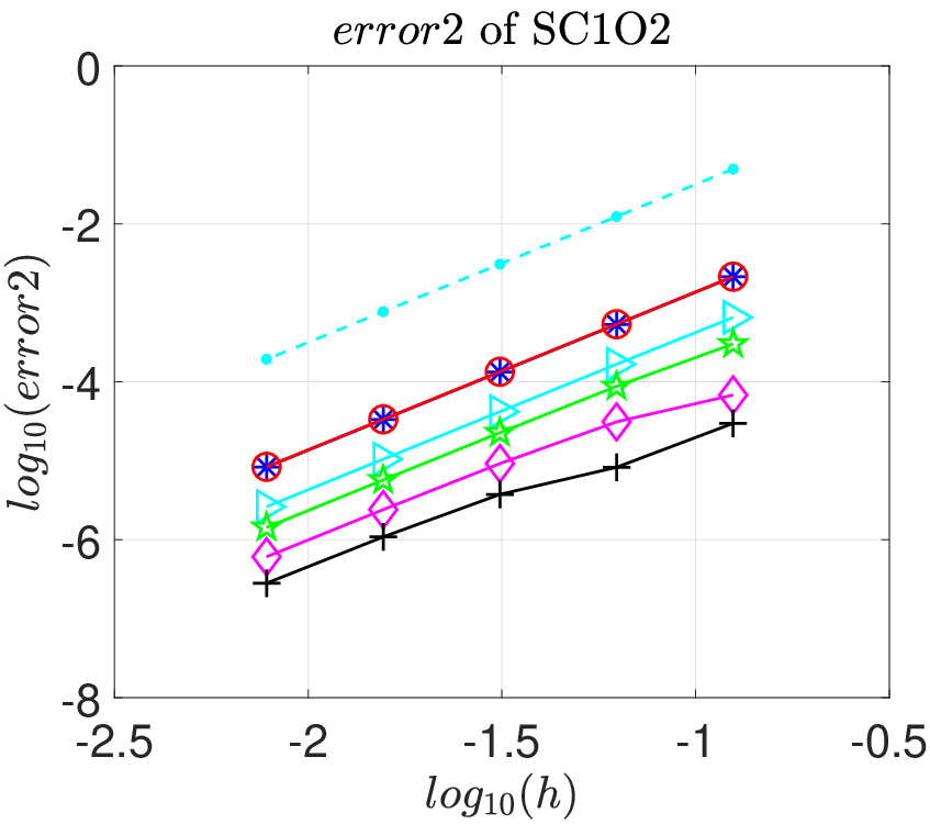
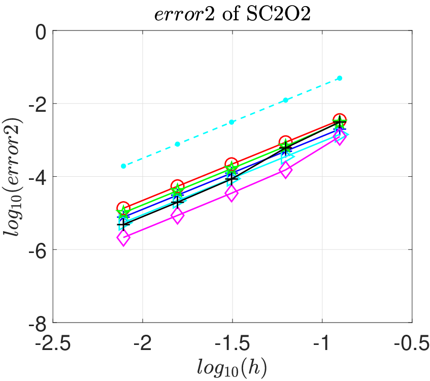
Problem 1. (Homogeneous magnetic field) This problem is devoted to the charged-particle system (1.1) of [21] with an additional factor $1/\epsilon$ and a homogeneous magnetic field. We take the scalar potential $U(x)=\frac{1}{100\sqrt{x_{1}^{2}+x_{2}^{2}}}$ , the homogeneous magnetic field $\frac{1}{\epsilon}B=\frac{1}{\epsilon}(0,0,1)^{\intercal}$ and the initial conditions as $x(0)=(0,0.2,0.1)^{\intercal},v(0)=(0.09,0.05,0.2)^{\intercal}.$

Order behaviour. This system is integrated on $[0,1]$ with different $\epsilon$ and step sizes $h$ to show the global errors $error$ in Fig. 1. According to the result, it can be seen that the global error lines of SC1O2 and SC2O2 are nearly parallel to the line with slope 2, which verifies that these two methods have second-order accuracy. Similarly, the fourth-order accuracy can be observed for SC1O4 and SC2O4. Moreover, we can see that the global errors of our methods are smaller than the other three methods especially with small $\epsilon$ . This demonstrates that our methods have better accuracy than others when solving CPD in a strong magnetic field.

Uniform errors. To display the influence of $\epsilon$ on the global errors, we show the error $error2:=\frac{\left\|x_{n}-x(t_{n})\right\|}{\left\|x(t_{n})\right\|}+\frac{\epsilon\left\|v_{n}-v(t_{n})\right\|}{\left\|v(t_{n})\right\|}$ for the second order methods in Fig. 2 and $error4:=\frac{\epsilon^{2}\left\|x_{n}-x(t_{n})\right\|}{\left\|x(t_{n})\right\|}+\frac{\epsilon^{3}\left\|v_{n}-v(t_{n})\right\|}{\left\|v(t_{n})\right\|}$ for the fourth order ones in Fig. 3. It can be observed from the results that our methods demonstrate the convergence stated in Theorem 3.4 and behave much better than the others.

Energy conservation. Then we solve the problem with $h=\frac{1}{100}$ on the interval $[0,1000]$ . Fig. 4 displays the results of energy conservation $err_{H}$ . It can be observed that for the normal magnetic field, all the methods have good energy conservation over long times and they behave similarly. For the case that $\epsilon$ is small, the energy error of those two Runge-Kutta methods (RKO2 and RKO4) increases slightly when $t$ goes large while the other methods have a good performance. Moreover, our methods display better accuracy in the energy preservation than the Boris method.

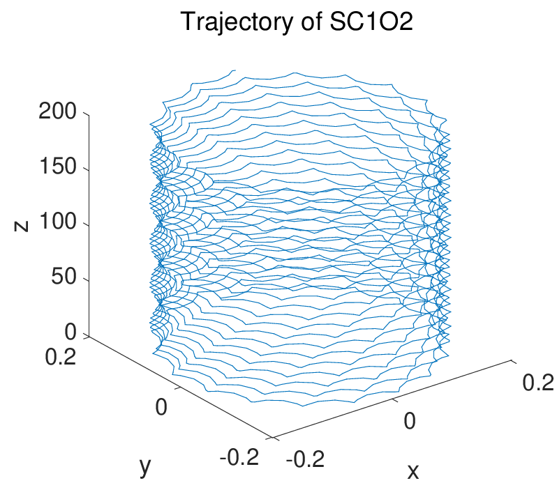
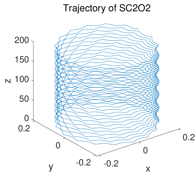
Long-time behavior. Finally, the problem is solved on $[0,1000]$ with $h=\frac{1}{2}$ and $\epsilon=0.1$ . Fig. 5 presents the trajectory for the second order methods (BORIS, RKO2, SC1O2 and SC2O2) in [x y z] space and the results show that the methods SC1O2 and SC2O2 perform uniformly better than the Boris and RKO2 methods. Meanwhile, we have noticed that the RKO2 method performs worse than expected. The reason is that for the RKO2 method when solving CPD with small $\epsilon$ , there is a very strict requirement of the stepsize and the method usually does not behave well.

Refer to caption — Figure 1. Problem 1. The global errors $error:=\frac{\left\|x_{n}-x(t_{n})\right\|}{\left\|x(t_{n})\right\|}+\frac{\left\|v_{n}-v(t_{n})\right\|}{\left\|v(t_{n})\right\|}$ with $t=1$ and $h=1/2^{k}$ for $k=3,4,\ldots,7$ under different $\epsilon$ .

4. Extension to CPD with non-homogeneous magnetic field

In this section, we consider the extension of the above symplectic methods and corresponding error estimates to the following CPD with a non-homogeneous magnetic field $B(x)$ :

\begin{array}[c]{ll}\ddot{x}=\dot{x}\times\frac{B(x)}{\epsilon}+F(x),\quad x(0)=x_{0},\quad\dot{x}(0)=\dot{x}_{0}.\end{array}

(4.1)

We remark that the above methods cannot be directly applied and some novel modifications are needed in the construction of the new methods.

4.1. Methods and their convergence

Algorithm 4.1.

(Adapted exponential methods) For solving the CPD (4.1) in a non-homogeneous magnetic field $B(x)$ , define the following continuous-stage adapted exponential method (denoted by SG1O1)

		$\displaystyle X_{\tau}=x_{n}+\tau h\varphi_{1}(\tau hM_{n})v_{n}+h^{2}\int_{0}^{1}\frac{\tau-\sigma}{2}\varphi_{1}((\tau-\sigma)hM_{n})F(X_{\sigma})d\sigma,$		(4.2)
		$\displaystyle x_{n+1}=x_{n}+h\varphi_{1}(hM_{n})v_{n}+h^{2}\int_{0}^{1}(1-\tau)\varphi_{1}((1-\tau)hM_{n})F(X_{\tau})d\tau,$
		$\displaystyle v_{n+1}=\varphi_{0}(hM_{n})v_{n}+h\int_{0}^{1}\varphi_{0}((1-\tau)hM_{n})F(X_{\tau})d\tau,$

with $M_{n}=\frac{1}{\epsilon}\tilde{B}(x_{n})$ .

The second scheme is obtained by considering another approximation of $\tilde{B}$ which leads to

		$\displaystyle X_{\tau}=x_{n}+\tau h\varphi_{1}(\tau h\tilde{M}_{n})v_{n}+h^{2}\int_{0}^{1}\frac{\tau-\sigma}{2}\varphi_{1}((\tau-\sigma)h\tilde{M}_{n})F(X_{\sigma})d\sigma,$		(4.3)
		$\displaystyle x_{n+1}=x_{n}+h\varphi_{1}(h\tilde{M}_{n})v_{n}+h^{2}\int_{0}^{1}(1-\tau)\varphi_{1}((1-\tau)h\tilde{M}_{n})F(X_{\tau})d\tau,$
		$\displaystyle v_{n+1}=\varphi_{0}(h\tilde{M}_{n})v_{n}+h\int_{0}^{1}\varphi_{0}((1-\tau)h\tilde{M}_{n})F(X_{\tau})d\tau,$

where $\tilde{M}_{n}=\frac{1}{\epsilon}\tilde{B}(\frac{x_{n}+x_{n+1}}{2})$ . We shall call it as SG1O2.

The third method is formulated as follows. Considering a Triple Jump splitting method [23] and denoting SG1O2 by $\Upsilon_{h}$ , then we get a splitting scheme: $\Phi_{h}=\Upsilon_{\kappa_{1}h}\circ\Upsilon_{\kappa_{2}h}\circ\Upsilon_{\kappa_{3}h}$ , where $\kappa_{1}=\kappa_{3}=\frac{1}{2-\sqrt[3]{2}}$ and $\kappa_{2}=-\frac{\sqrt[3]{2}}{2-\sqrt[3]{2}}$ . We denote this method by SG1O4.

The following theorem states the convergence of the above three methods.

Theorem 4.2.

(Convergence) For the CPD (4.1), we assume that its solution is sufficiently smooth, and the function $F$ is locally Lipschitz-continuous and sufficient differentiable. Under these conditions and $h\leq C\epsilon$ , the global errors of SG1O1, SG1O2 and SG1O4 are respectively given by


		$\displaystyle\textmd{SG1O1}:\quad\\|x(t_{n+1})-x_{n+1}\\|\leq Ch,\qquad\qquad\\|v(t_{n+1})-v_{n+1}\\|\leq Ch/\epsilon,$		(4.4a)
		$\displaystyle\textmd{SG1O2}:\quad\\|x(t_{n+1})-x_{n+1}\\|\leq Ch^{2}/\epsilon,\qquad\ \ \\|v(t_{n+1})-v_{n+1}\\|\leq Ch^{2}/\epsilon^{2},$		(4.4b)
		$\displaystyle\textmd{SG1O4}:\quad\\|x(t_{n+1})-x_{n+1}\\|\leq Ch^{4}/\epsilon^{3},\qquad\ \\|v(t_{n+1})-v_{n+1}\\|\leq Ch^{4}/\epsilon^{4},$		(4.4c)

where $0<n<T/h$ and the generic constant $C>0$ is independent of $\epsilon,\ h,\ n$ .

Proof.

The proof is firstly given for the errors of SG1O2 and then the results of the other methods can be derived with similar procedure.

$\bullet$ Proof of (4.4b). Linearized system. The first step is to rewrite the system (4.1) as

\displaystyle\dot{x}=v,\ \ \dot{v}=v\times\frac{B(x)}{\epsilon}+F(x),\ \ x(0)=x_{0},\ \ v(0)=v_{0}.

(4.5)

For some $t=t_{n}+s$ with $n\geq 0$ , we consider the following linearized system of (4.5)

\displaystyle\dot{\tilde{x}}_{n}(s)=\dot{\tilde{v}}_{n}(s),\ \ \dot{\tilde{v}}_{n}(s)=\frac{1}{\epsilon}\tilde{B}(x_{n+\frac{1}{2}})\tilde{v}_{n}(s)+F({\tilde{x}}_{n}(s)),\ \ {\tilde{x}}_{n}(0)=x(t_{n}),\ \ {\tilde{v}}_{n}(0)=v(t_{n}),\ \ \ 0<s\leq h,

(4.6)

where $x_{n+\frac{1}{2}}=\frac{x(t_{n})+x(t_{n+1})}{2}$ .

Local errors between the original and linearized systems. Then we denote the local errors between the above two systems by

\xi^{x}_{n}(s)=x(t_{n}+s)-\tilde{x}_{n}(s),\ \ \xi^{v}_{n}(s)=v(t_{n}+s)-\tilde{v}_{n}(s),\ \ \ \ 0\leq n<\frac{T}{h}.

It is easily obtained from (4.5) and (4.6) that

\displaystyle\dot{\xi}^{x}_{n}(s)=\xi^{v}_{n}(s),\ \ \dot{\xi}^{v}_{n}(s)=\frac{1}{\epsilon}\tilde{B}(x_{n+\frac{1}{2}})\xi^{v}_{n}(s)+F(x(t_{n}+s))-F(\tilde{x}_{n}(s))+\varsigma^{0}_{n}(s).

(4.7)

Here we denote $\varsigma^{0}_{n}(s)=\frac{1}{\epsilon}\big(\tilde{B}\big(x(t_{n}+s)\big)-\tilde{B}\big(x_{n+\frac{1}{2}}\big)\big)v(t_{n}+s)$ , and using the Taylor expansion yields

		$\displaystyle\tilde{B}(x(t_{n}+s))-\tilde{B}\big(x_{n+\frac{1}{2}}\big)=\tilde{B}(x(t_{n}))+\frac{d\tilde{B}}{dx}(\dot{x}(t_{n})s+\mathcal{O}(s^{2}/\epsilon))+{\mathcal{O}(s^{3}/\epsilon)}-\tilde{B}(x(t_{n}))$
		$\displaystyle-\frac{d\tilde{B}}{dx}(\dot{x}(t_{n})h/2+\mathcal{O}(h^{2}/\epsilon))-\mathcal{O}(h^{2}/\epsilon)=\tilde{B}^{(1)}_{n}(s-h/2)+\mathcal{O}(h^{2}/\epsilon),$

where $\tilde{B}^{(i)}_{n}=\frac{d^{i}}{dt^{i}}\tilde{B}(x(t))\mid_{t=t_{n}},\ \ i=1,2$ . Likewise, we get

v(t_{n}+s)=v(t_{n})+\dot{v}(t_{n})s+\mathcal{O}(s^{2}/\epsilon^{2}).

Combining the above two formulae, one arrives at

\displaystyle\varsigma^{0}_{n}(s)=\frac{1}{\epsilon}\tilde{B}_{n}^{(1)}(s-h/2)v(t_{n})+\frac{1}{\epsilon}\tilde{B}_{n}^{(1)}s(s-h/2)\dot{v}(t_{n})+\mathcal{O}(h^{2}/\epsilon^{2}).

(4.8)

Then taking the variation-of-constant formula of (4.7) into account, we have that

\displaystyle\xi^{x}_{n}(h)=\int_{0}^{h}\xi^{v}_{n}(s)ds,\ \ \xi^{v}_{n}(h)=\int_{0}^{h}e^{\frac{h-s}{\epsilon}\tilde{B}(x_{n+\frac{1}{2}})}\bigg(\int_{0}^{1}\nabla F(x(t_{n}+s)+(\sigma-1)\xi^{x}_{n}(s))\xi^{x}_{n}(s)d\sigma+\varsigma^{0}_{n}(s)\bigg)ds,

which further gives

		$\displaystyle\xi^{x}_{n}(h)=\int_{0}^{h}\int_{0}^{s}e^{\frac{s-\delta}{\epsilon}\tilde{B}(x_{n+\frac{1}{2}})}\int_{0}^{1}\nabla F(x(t_{n}+\delta)+(\sigma-1)\xi^{x}_{n}(\delta))\xi^{x}_{n}(s)d\sigma d\delta ds$		(4.9)
		$\displaystyle+\int_{0}^{h}\int_{0}^{s}e^{\frac{s-\delta}{\epsilon}\tilde{B}(x_{n+\frac{1}{2}})}\varsigma^{0}_{n}(\delta)d\delta ds.$		(4.9)

Inserting the formula (4.8) into the second part of (4.9), we get

		$\displaystyle\int_{0}^{h}\int_{0}^{s}e^{\frac{s-\delta}{\epsilon}\tilde{B}(x_{n+\frac{1}{2}})}\varsigma^{0}_{n}(\delta)d\delta ds=\underbrace{\frac{1}{\epsilon}\int_{0}^{h}\int_{0}^{s}e^{\frac{s-\delta}{\epsilon}\tilde{B}(x_{n+\frac{1}{2}})}B_{n}^{(1)}(\delta-h/2)v(t_{n})d\delta ds}_{\textmd{part}\ I}$
		$\displaystyle+\underbrace{\frac{1}{\epsilon}\int_{0}^{h}\int_{0}^{s}e^{\frac{s-\delta}{\epsilon}\tilde{B}(x_{n+\frac{1}{2}})}B_{n}^{(1)}\delta(\delta-h/2)\dot{v}(t_{n})d\delta ds}_{\textmd{part}\ II}+\mathcal{O}(h^{4}/\epsilon^{2}).$

With some calculations, it is easy to have that

\textmd{part}\ I=\mathcal{O}(h^{3}/\epsilon),\quad\textmd{part}\ II=\mathcal{O}(h^{5}/\epsilon^{2}).

Considering further that $h\leq C\epsilon$ , we get $\int_{0}^{h}\int_{0}^{s}e^{\frac{s-\delta}{\epsilon}\tilde{B}(x_{n+\frac{1}{2}})}\varsigma^{0}_{n}(\delta)d\delta ds=\mathcal{O}(h^{3}/\epsilon).$ Hence, the local error $\xi^{x}_{n}(h)$ is bounded by

\xi^{x}_{n}(h)=\mathcal{O}(h^{3}/\epsilon).

(4.10)

In the same way, it is arrived that

		$\displaystyle\int_{0}^{h}e^{\frac{h-s}{\epsilon}\tilde{B}(x_{n+\frac{1}{2}})}\varsigma^{0}_{n}(s)ds=\frac{1}{\epsilon}\int_{0}^{h}e^{\frac{h-s}{\epsilon}\tilde{B}(x_{n+\frac{1}{2}})}v(t_{n})(s-h/2)B_{n}^{(1)}ds$
		$\displaystyle+\frac{1}{\epsilon}\int_{0}^{h}e^{\frac{h-s}{\epsilon}\tilde{B}(x_{n+\frac{1}{2}})}\dot{v}(t_{n})s(s-h/2)B_{n}^{(1)}ds+\mathcal{O}(h^{3}/\epsilon^{2})=\mathcal{O}(h^{3}/\epsilon^{2}),$

and based on which, we thus have

\xi^{v}_{n}(h)=\mathcal{O}(h^{3}/\epsilon^{2}).

(4.11)

Global errors. With the above analysis, we shall estimate the global errors of the method (4.3), i.e.,

e^{x}_{n+1}:=x(t_{n+1})-x_{n+1},\ \ \ e^{v}_{n+1}:=v(t_{n+1})-v_{n+1}.

These errors can be split into two parts

e^{x}_{n+1}=\tilde{e}^{x}_{n}+\xi^{x}_{n}(h),\ \ \ e^{v}_{n+1}=\tilde{e}^{v}_{n}+\xi^{v}_{n}(h),

(4.12)

and then converted to evaluate

\tilde{e}^{x}_{n}:=\tilde{x}_{n}(h)-x_{n+1},\ \ \ \tilde{e}^{v}_{n}:=\tilde{v}_{n}(h)-v_{n+1}.

On the basis of the method (4.3), we present the local error $\varphi_{n}^{x}$ and $\varphi_{n}^{v}$ as follows

		$\displaystyle\tilde{x}_{n}(\tau h)=\tilde{x}_{n}(0)+\tau h\varphi_{1}\big(\tau h\tilde{P}\big)\tilde{v}_{n}(0)+h^{2}\int_{0}^{1}\frac{\tau-\sigma}{2}\varphi_{1}\big((\tau-\sigma)h\tilde{P}\big)F(\tilde{x}_{n}(\sigma h))d\sigma+\varphi_{n}^{\tau},$		(4.13)
		$\displaystyle\tilde{x}_{n}(h)=\tilde{x}_{n}(0)+h\varphi_{1}\big(h\tilde{P}\big)\tilde{v}_{n}(0)+h^{2}\int_{0}^{1}(1-\tau)\varphi_{1}\big((1-\tau)h\tilde{P}\big)F(\tilde{x}_{n}(\tau h))d\tau+\varphi_{n}^{x},$
		$\displaystyle\tilde{v}_{n}(h)=\varphi_{0}\big(h\tilde{P}\big)\tilde{v}_{n}(0)+h\int_{0}^{1}\varphi_{0}\big((1-\tau)h\tilde{P}\big)F(\tilde{x}_{n}(\tau h))d\tau+\varphi_{n}^{v},$

where $\tilde{P}=\frac{1}{\epsilon}\tilde{B}\Big(\frac{\tilde{x}_{n}(0)+\tilde{x}_{n}(h)}{2}\Big)$ . It follows from the variation-of-constant formula of the linearized system (4.6) that

		$\displaystyle\tilde{x}_{n}(\tau h)=\tilde{x}_{n}(0)+\tau h\varphi_{1}(\tau hP)\tilde{v}_{n}(0)+h^{2}\int_{0}^{\tau}(\tau-\sigma)\varphi_{1}((\tau-\sigma)hP)F(\tilde{x}_{n}(\sigma h))d\sigma,$		(4.14)
		$\displaystyle\tilde{x}_{n}(h)=\tilde{x}_{n}(0)+h\varphi_{1}(hP)\tilde{v}_{n}(0)+h^{2}\int_{0}^{1}(1-\tau)\varphi_{1}((1-\tau)hP)F(\tilde{x}_{n}(\tau h))d\tau,$
		$\displaystyle\tilde{v}_{n}(h)=\varphi_{0}(hP)\tilde{v}_{n}(0)+h\int_{0}^{1}\varphi_{0}((1-\tau)hP)F(\tilde{x}_{n}(\tau h))d\tau,$

where $P=\frac{1}{\epsilon}\tilde{B}\Big(\frac{x(t_{n})+x(t_{n+1})}{2}\Big)$ . Considering the difference between (4.13) and (4.14), we get

	$\displaystyle\varphi_{n}^{\tau}$	$\displaystyle=\tau h\big(\varphi_{1}(\tau hP)-\varphi_{1}(\tau h\tilde{P})\big){v}(t_{n})+\tau^{2}h^{2}\int_{0}^{1}(1-z)\varphi_{1}\big(\tau(1-z)hP\big)F\big(\tilde{x}_{n}(h\tau z)\big)dz$
		$\displaystyle-h^{2}\int_{0}^{1}\frac{(\tau-\sigma)}{2}\varphi_{1}\big((\tau-\sigma)h\tilde{P}\big)F\big(\tilde{x}_{n}(\sigma h)\big)d\sigma,$
	$\displaystyle\varphi_{n}^{x}$	$\displaystyle=h\big(\varphi_{1}(hP)-\varphi_{1}(h\tilde{P})\big){v}(t_{n})+h^{2}\int_{0}^{1}(1-\tau)\big(\varphi_{1}\big((1-\tau)hP\big)-\varphi_{1}\big((1-\tau)h\tilde{P}\big)\big)F\big(\tilde{x}_{n}(\tau h)\big)d\tau,$
	$\displaystyle\varphi_{n}^{v}$	$\displaystyle=\big(\varphi_{0}(hP)-\varphi_{0}(h\tilde{P})\big){v}(t_{n})+h\int_{0}^{1}\big(\varphi_{0}\big((1-\tau)hP\big)-\varphi_{0}\big((1-\tau)h\tilde{P}\big)\big)F\big(\tilde{x}_{n}(\tau h)\big)d\tau.$

Similarly as the analysis of Theorem 3.4, it follows that

\left\|\varphi_{n}^{\tau}\right\|=\mathcal{O}(h^{2}),\qquad\ \left\|\varphi_{n}^{x}\right\|=\mathcal{O}(h^{3}/\epsilon),\qquad\ \left\|\varphi_{n}^{v}\right\|=\mathcal{O}(h^{3}/\epsilon).

(4.15)

Subtracting (4.3) from (4.13) and by further using (4.12), we have

\displaystyle{\displaystyle e}^{x}_{n+1}={e}^{x}_{n}+h\varphi_{1}(h\tilde{P}){e}^{v}_{n}+\varphi_{n}^{x}+\xi^{x}_{n}(h)+\gamma_{n}^{x},\ \ \ \ {e}^{v}_{n+1}=\varphi_{0}(h\tilde{P}){e}^{v}_{n}+\varphi_{n}^{v}+\xi^{v}_{n}(h)+\gamma_{n}^{v},

where

		$\displaystyle\gamma_{n}^{x}=h\big(\varphi_{1}(h\tilde{P})-\varphi_{1}(h\tilde{M}_{n})\big)v_{n}+h^{2}\int_{0}^{1}(1-\tau)\varphi_{1}\big((1-\tau)h\tilde{P}\big)\big(F(\tilde{x}_{n}(\tau h))-F(X_{\tau})\big)d\tau$
		$\displaystyle+h^{2}\int_{0}^{1}(1-\tau)\big(\varphi_{1}\big((1-\tau)h\tilde{P}\big)-\varphi_{1}\big((1-\tau)h\tilde{M}_{n}\big)\big)F(X_{\tau})d\tau,$
		$\displaystyle\gamma_{n}^{v}=\big(\varphi_{0}(h\tilde{P})-\varphi_{0}(h\tilde{M}_{n})\big)v_{n}+h\int_{0}^{1}\varphi_{0}\big((1-\tau)h\tilde{P}\big)\big(F(\tilde{x}_{n}(\tau h))-F(X_{\tau})\big)d\tau$
		$\displaystyle+h\int_{0}^{1}\big(\varphi_{0}\big((1-\tau)h\tilde{P}\big)-\varphi_{0}\big((1-\tau)h\tilde{M}_{n}\big)\big)F(X_{\tau})d\tau.$

Considering the same process of deduction in Theorem 3.4, one gets

\displaystyle\left\|\gamma_{n}^{x}\right\|\leq\frac{h^{2}}{\epsilon}(\|e_{n}^{x}\|+h\|e_{n}^{v}\|+\|e_{n+1}^{x}\|+\|\xi_{n}^{x}(h)\|),

\displaystyle\left\|\gamma_{n}^{v}\right\|\leq\frac{h}{\epsilon}(\|e_{n}^{x}\|+h\|e_{n}^{v}\|+\|e_{n+1}^{x}\|+\|\xi_{n}^{x}(h)\|).

We then obtain

	$\displaystyle\left\\|e_{n+1}^{x}\right\\|$	$\displaystyle\leq\left\\|e_{n}^{x}\right\\|+h\left\\|e_{n}^{v}\right\\|+\left\\|\varphi_{n}^{x}\right\\|+\left\\|\xi_{n}^{x}(h)\right\\|+\left\\|\gamma_{n}^{x}\right\\|$
		$\displaystyle\leq\left\\|e_{n}^{x}\right\\|+h\big(\left\\|e_{n}^{x}\right\\|+\left\\|e_{n}^{v}\right\\|+\left\\|e_{n+1}^{x}\right\\|\big)+\left\\|\varphi_{n}^{x}\right\\|+\left\\|\xi_{n}^{x}(h)\right\\|,$

and

	$\displaystyle\left\\|e_{n+1}^{v}\right\\|$	$\displaystyle\leq\left\\|e_{n}^{v}\right\\|+\left\\|\varphi_{n}^{v}\right\\|+\left\\|\xi_{n}^{v}(h)\right\\|+\left\\|\gamma_{n}^{v}\right\\|$
		$\displaystyle\leq\left\\|e_{n}^{v}\right\\|+\frac{h}{\epsilon}\big(\left\\|e_{n}^{x}\right\\|+\left\\|e_{n}^{v}\right\\|+\left\\|e_{n+1}^{x}\right\\|\big)+\left\\|\varphi_{n}^{v}\right\\|+\left\\|\xi_{n}^{v}(h)\right\\|.$

Combining $\left\|e_{n+1}^{x}\right\|$ and $\epsilon\left\|e_{n+1}^{v}\right\|$ , we have

		$\displaystyle\left\\|e_{n+1}^{x}\right\\|+\epsilon\left\\|e_{n+1}^{v}\right\\|-\left\\|e_{n}^{x}\right\\|-\epsilon\left\\|e_{n}^{v}\right\\|$
	$\displaystyle\leq$	$\displaystyle h(\\|e_{n}^{x}\\|+\\|e_{n}^{v}\\|+\\|e_{n+1}^{x}\\|)+\left\\|\varphi_{n}^{x}\right\\|+\epsilon\left\\|\varphi_{n}^{v}\right\\|+\left\\|\xi_{n}^{x}(h)\right\\|+\epsilon\left\\|\xi_{n}^{v}(h)\right\\|.$

Further, using recursion formula and $e_{0}^{x}=e_{0}^{v}=0$ , it is arrived that

\displaystyle\left\|e_{n+1}^{x}\right\|+\epsilon\left\|e_{n+1}^{v}\right\|\leq h\sum_{m=0}^{n}(\|e_{m}^{x}\|+\|e_{m}^{v}\|+\|e_{m+1}^{x}\|)+\sum_{m=0}^{n}(\left\|\varphi_{m}^{x}\right\|+\epsilon\left\|\varphi_{m}^{v}\right\|+\left\|\xi_{m}^{x}(h)\right\|+\epsilon\left\|\xi_{m}^{v}(h)\right\|).

By inserting the errors (4.10), (4.11) and (4.15) into the above formula and using the fact that $nh<T$ , one has

\displaystyle\left\|e_{n+1}^{x}\right\|+\epsilon\left\|e_{n+1}^{v}\right\|\leq h\sum_{m=0}^{n}(\|e_{m}^{x}\|+\|e_{m}^{v}\|+\|e_{m+1}^{x}\|)+Ch^{2}/\epsilon.

Using the Gronwall’s inequality, we get

\displaystyle\left\|e_{n+1}^{x}\right\|+\epsilon\left\|e_{n+1}^{v}\right\|\leq Ch^{2}/\epsilon.

Therefore, the global error (4.4b) of the method (4.3) is obtained immediately.

$\bullet$ Proof of (4.4a). This proof is also divided into three parts as the analysis of (4.4b).

Firstly, we denote the linearized system of (4.5) as

\displaystyle\dot{\tilde{x}}_{n}(s)=\dot{\tilde{v}}_{n}(s),\ \dot{\tilde{v}}_{n}(s)=\frac{1}{\epsilon}\tilde{B}(x(t_{n}))\tilde{v}_{n}(s)+F({\tilde{x}}_{n}(s)),\ {\tilde{x}}_{n}(0)=x(t_{n}),\ {\tilde{v}}_{n}(0)=v(t_{n}),\ 0<s\leq h.

(4.16)

Then the local errors between the original (4.5) and linearized systems (4.16) are given by

\xi^{x}_{n}(h)=\mathcal{O}(h^{2}),\qquad\xi^{v}_{n}(h)=\mathcal{O}(h^{2}/\epsilon),

which can be obtained in the same way by the proof of (4.4b).

Finally, according to the above analysis, we get the final conclusion as follows

\left\|e_{n+1}^{x}\right\|+\epsilon\left\|e_{n+1}^{v}\right\|\leq Ch,

which proves the result of (4.4a).

$\bullet$ Proof of (4.4c). It is noted that the error bound between the system (4.5) and linearized system (4.6) is $\mathcal{O}(h^{2})$ . Thus higher order methods can not be obtained by considering algorithms with higher order for the linearized system (4.6). That is the reason why we use the idea of Triple Jump splitting method to construct the fourth-order method SG1O4. The convergence of this splitting can be derived by the standard analysis (see, e.g., [23]) and we omit it for brevity.

The proof of the theorem is finished.∎

For the special but important magnetic field, the so-called maximal ordering scaling [7, 24, 36]:

\displaystyle\dot{x}=v,\ \ \dot{v}=v\times\frac{B(\epsilon x)}{\epsilon}+F(x),\ \ x(0)=x_{0},\ \ v(0)=v_{0},

(4.17)

the improved convergent results can be obtained which are shown as follows.

Theorem 4.3.

(Improved error bounds) Under the conditions of Theorem 4.2, if the magnetic field has the maximal ordering scaling, i.e., $B=B(\epsilon x)$ , we have the following improved error bounds


		$\displaystyle\textmd{SG1O1}:\quad\left\\|x(t_{n+1})-x_{n+1}\right\\|\leq Ch,\quad\quad\ \ \ \left\\|v(t_{n+1})-v_{n+1}\right\\|\leq Ch,$		(4.18a)
		$\displaystyle\textmd{SG1O2}:\quad\left\\|x(t_{n+1})-x_{n+1}\right\\|\leq Ch^{2},\qquad\ \ \left\\|v(t_{n+1})-v_{n+1}\right\\|\leq Ch^{2}/\epsilon,$		(4.18b)
		$\displaystyle\textmd{SG1O4}:\quad\left\\|x(t_{n+1})-x_{n+1}\right\\|\leq Ch^{4}/\epsilon^{2},\quad\ \left\\|v(t_{n+1})-v_{n+1}\right\\|\leq Ch^{4}/\epsilon^{3}.$		(4.18c)

Proof.

$\bullet$ Proof of (4.18a). Concern the linearized system of (4.17) as follows

\displaystyle\dot{\tilde{x}}_{n}(s)=\dot{\tilde{v}}_{n}(s),\ \ \dot{\tilde{v}}_{n}(s)=\frac{1}{\epsilon}\tilde{B}(\epsilon x(t_{n}))\tilde{v}_{n}(s)+F({\tilde{x}}_{n}(s)),\ \ {\tilde{x}}_{n}(0)=x(t_{n}),\ \ {\tilde{v}}_{n}(0)=v(t_{n}),\ \ \ 0<s\leq h.

(4.19)

Similarly as the proof of Theorem 4.2, the errors between the systems (4.17) and (4.19) are bounded as follows

\xi^{x}_{n}(h)=\mathcal{O}(h^{3}),\ \ \ \ \ \ \ \xi^{v}_{n}(h)=\mathcal{O}(h^{3}/\epsilon).

Then, we shall consider the global errors of the method (4.2) in the same way as Theorem 4.2, and one gets

		$\displaystyle\left\\|{e}^{x}_{n+1}\right\\|\leq\left\\|{e}^{x}_{n}\right\\|+h\left\\|{e}^{v}_{n}\right\\|+\left\\|\varphi_{n}^{x}\right\\|+\left\\|\xi^{x}_{n}(h)\right\\|+\left\\|\gamma_{n}^{x}\right\\|,$
		$\displaystyle\left\\|{e}^{v}_{n+1}\right\\|\leq\left\\|{e}^{v}_{n}\right\\|+\left\\|\varphi_{n}^{v}\right\\|+\left\\|\xi^{v}_{n}(h)\right\\|+\left\\|\gamma_{n}^{v}\right\\|.$

The notations $\varphi_{n}^{x}$ , $\varphi_{n}^{v}$ , $\gamma_{n}^{x}$ and $\gamma_{n}^{v}$ are totally the same as those in the proof of (4.4b) with some corresponding modifications in $B$ . They are bounded by

\left\|\varphi_{n}^{x}\right\|=\mathcal{O}(h^{3}/\epsilon),\ \ \left\|\varphi_{n}^{v}\right\|=\mathcal{O}(h^{3}/\epsilon),\ \ \left\|\gamma_{n}^{x}\right\|\leq h^{2}(\left\|e_{n}^{x}\right\|+h\left\|e_{n}^{v}\right\|),\ \ \left\|\gamma_{n}^{v}\right\|\leq h(\left\|e_{n}^{x}\right\|+h\left\|e_{n}^{v}\right\|).

The above results lead to

\displaystyle\left\|{e}^{x}_{n+1}\right\|+\left\|{e}^{v}_{n+1}\right\|-\left\|{e}^{x}_{n}\right\|-\left\|{e}^{v}_{n}\right\|\leq h(\left\|{e}^{x}_{n}\right\|+\left\|{e}^{v}_{n}\right\|)+\left\|\varphi_{n}^{x}\right\|+\left\|\varphi_{n}^{v}\right\|+\left\|\xi_{n}^{x}(h)\right\|+\left\|\xi_{n}^{v}(h)\right\|.

Therefore, we have

\left\|e_{n+1}^{x}\right\|+\left\|e_{n+1}^{v}\right\|\leq Ch.

$\bullet$ Proof of (4.18b)–(4.18c). The proof of (4.18b) and (4.18c) can be obtained by the same progress with (4.18a), and so we leave out the details for simplicity. ∎

4.2. Numerical tests

In what follows, we present two numerical experiments to show the behaviour of the derived methods. We still choose BORIS, RKO2 and RKO4 for comparison which are given in Section 3.4. To compare the first order method SG1O1 with some existing methods, the implicit Euler method (of order one) is chosen and we refer to it as Euler.

Problem 2. (General magnetic field) For the charged-particle dynamics (1.1), the scalar potential $U(x)$ and non-homogeneous magnetic field $\frac{1}{\epsilon}B(x)$ are given by ([21])

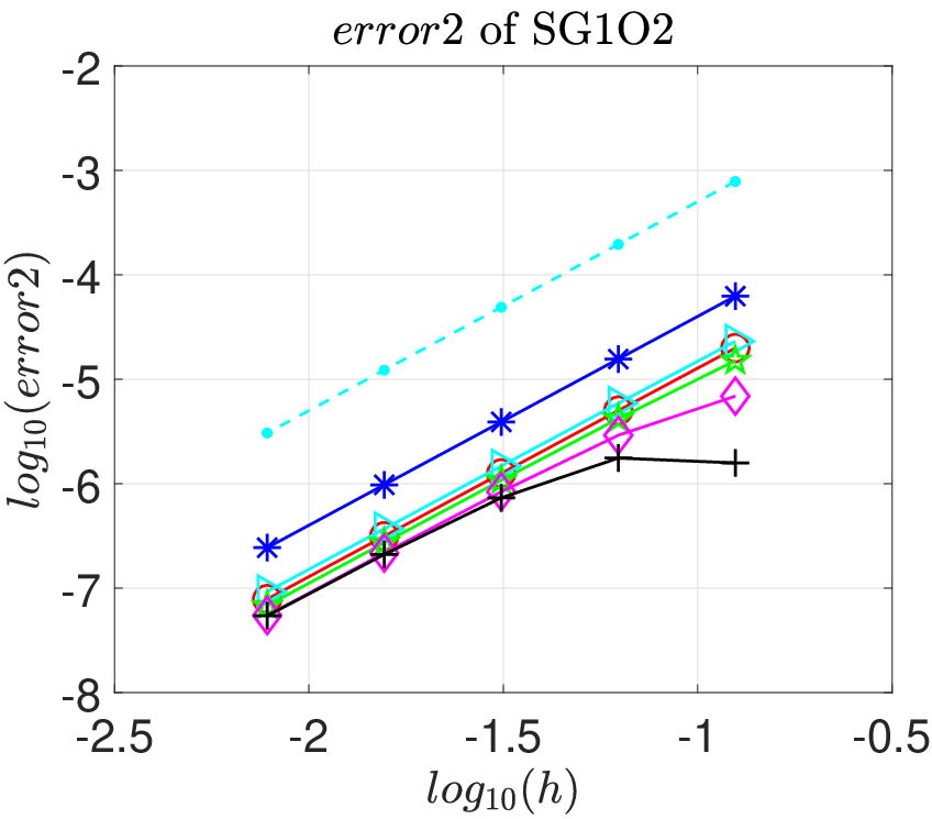
\frac{1}{\epsilon}B(x)=\nabla\times\frac{1}{3\epsilon}\Big(-x_{2}\sqrt{x_{1}^{2}+x_{2}^{2}},x_{1}\sqrt{x_{1}^{2}+x_{2}^{2}},0\Big)^{T}=\frac{1}{\epsilon}\Big(0,0,\sqrt{x_{1}^{2}+x_{2}^{2}}\Big)^{\intercal},\ \ \ U(x)=\frac{1}{100\sqrt{x_{1}^{2}+x_{2}^{2}}},

where initial values are chosen as $x(0)=(0,1,0.1)^{\intercal},\ v(0)=(0.09,0.05,0.2)^{\intercal}.$ The problem is solved on $[0,1]$ with $h=1/2^{k},$ where $k=3,\ldots,7$ , and Figs. 6–9 show the results of global errors. Then the system is integrated on the interval $[0,100]$ with a step size $h=\frac{1}{100}$ and see Fig. 10 for the energy conservation.

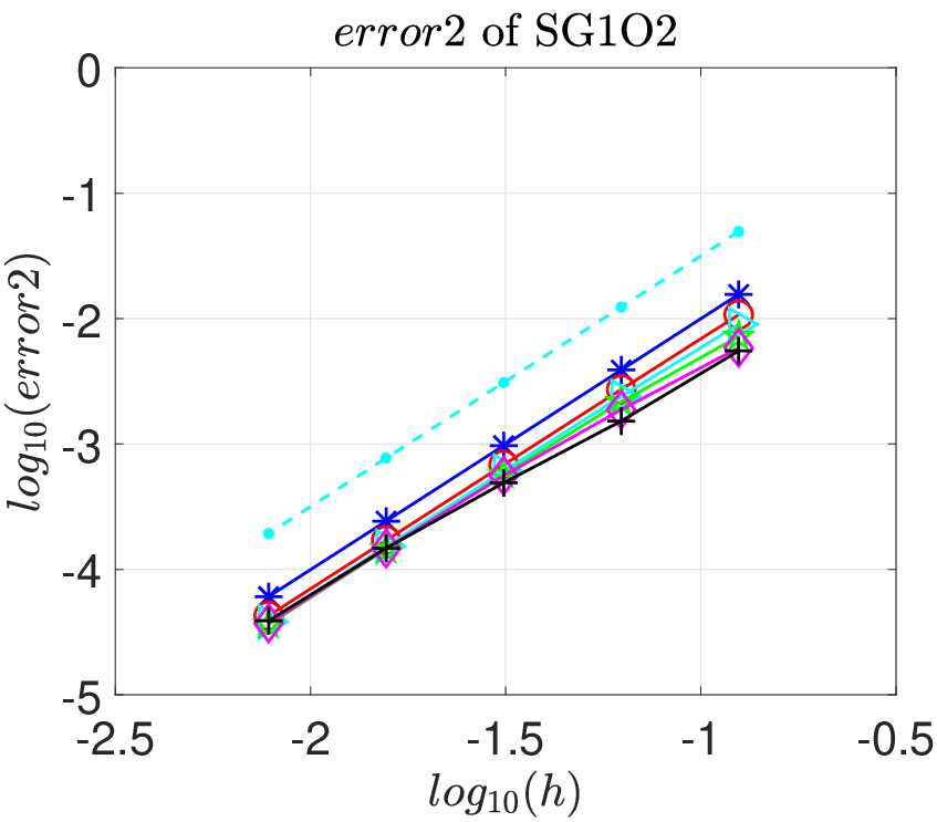
Problem 3. (Maximal ordering scaling) Consider the charged-particle dynamics (1.1) from [47] in a magnetic field with the maximal ordering scaling $\frac{1}{\epsilon}B(\epsilon x)=\frac{1}{\epsilon}\left(\begin{array}[]{c}\cos(\epsilon x_{2})\\ 1+\sin(\epsilon x_{3})\\ \cos(\epsilon x_{1})\\ \end{array}\right)+\left(\begin{array}[]{c}-x_{1}\\ 0\\ x_{3}\\ \end{array}\right)$ and the scalar potential $U(x)=\frac{1}{\sqrt{x_{1}^{2}+x_{2}^{2}}}.$ We take $x(0)=(1/3,1/4,1/2)^{\intercal},\ v(0)=(2/5,2/3,1)^{\intercal}$ as the initial values. Figs. 11–14 present the errors of all the methods when solving this problem on $[0,1]$ with different $\epsilon$ and $h=1/2^{k}$ , where $k=3,4,\ldots,7$ . Finally, the energy errors are shown in Fig. 15 on $[0,100]$ with $h=\frac{1}{20}$ .

Based on the above results, we can draw the following observations. For the accuracy, our methods agree with the results presented in Theorem 4.2 and 4.3 and are more accurate than the Euler, Boris and Runge-Kutta methods. Concerning the energy conservation, it can be seen that our methods have a long time conservation not only for normal magnetic fields but also for strong ones.

5. Conclusions

In this paper, symplectic methods for solving the charged-particle dynamics (CPD) (1.1) were presented and studied. By employing some transformations of the system and methods, we derived symplecticity conditions for a novel kind of adapted exponential methods, and based on which, two symplectic methods up to order four were constructed for solving CPD in a strong and homogeneous magnetic field. Rigorous error estimates were presented and the proposed second order symplectic method was shown to have uniform error bound in the position w.r.t. the strength of the magnetic field. Furthermore, the extension of the obtained symplectic methods to the case of non-homogeneous magnetic fields was discussed. Three novel algorithms up to order four were constructed and one method was proved to have uniform accuracy in the position. Some numerical tests on homogeneous and non-homogeneous magnetic fields were presented to confirm the theoretical results and to demonstrate the numerical behaviour in accuracy and energy conservation.

Last but not least, we point out that the numerical results of Problems 1–3 demonstrate a very good long time energy conservation for the methods presented in this paper. To theoretically prove this property, the strategies named as backward error analysis [20, 21, 23, 46] and modulated Fourier expansion [19, 22, 23, 24, 47] will be employed for CPD under normal and strong magnetic fields, respectively. The rigorous analysis on this topic will be considered in our next work. Another issue for future exploration is the study of uniform higher-order symplectic integrators. Besides, a combination of symplectic integrators and the Particle-In-Cell (PIC) approximation and its analysis are of great interests for Vlasov equations [11, 12, 14, 15, 16].

References

[1] V.I. Arnold, V.V. Kozlov, A.I. Neishtadt, Mathematical Aspects of Classical and Celestial Mechanics, Springer, Berlin, 1997.
[2] W. Bao, C. Su, A uniformly and optimally accurate methods for the Zakharov system in the subsonic limit regime, SIAM J. Sci. Comput. 40 (2018), pp. A929-A953.
[3] W. Bao, Q. Zhao, A structure-preserving parametric finite element method for surface diffusion, SIAM J. Numer. Anal. 59 (2021), pp. 2775–2799.
[4] G. Benettin, P. Sempio, Adiabatic invariants and trapping of a point charge in a strong nonhomogeneous magnetic field, Nonlinearity 7 (1994), pp. 281-304.
[5] S. Blanes, A. Iserles, Explicit adaptive symplectic integrators for solving Hamiltonian systems, Celest. Mech. Dyn. Astron. 114 (2012), pp. 297–317.
[6] J.P. Boris, Relativistic plasma simulation-optimization of a hybird code, Proceeding of Fourth Conference on Numerical Simulations of Plasmas (1970), pp. 3-67.
[7] A.J. Brizard, T.S. Hahm, Foundations of nonlinear gyrokinetic Theory, Rev. Modern Phys. 79 (2007), pp. 421-468.
[8] L. Brugnano, F. Iavernaro, R. Zhang, Arbitrarily high-order energy-preserving methods for simulating the gyrocenter dynamics of charged particles, J. Comput. Appl. Math. 380 (2020), pp. 112994.
[9] L. Brugnano, J.I. Montijano, L. Rándz, High-order energy-conserving line integral methods for charged particle dynamics, J. Comput. Phys. 396 (2019), pp. 209-227.
[10] J.R. Cary, A.J. Brizard, Hamiltonian theory of guiding-center motion, Rev. Modern Phys. 81 (2009), pp. 693-738.
[11] Ph. Chartier, N. Crouseilles, M. Lemou, F. Méhats, X. Zhao, Uniformly accurate methods for Vlasov equations with non-homogeneous strong magnetic field, Math. Comp. 88 (2019), pp. 2697-2736.
[12] Ph. Chartier, N. Crouseilles, M. Lemou, F. Méhats, X. Zhao, Uniformly accurate methods for three dimensional Vlasov equations under strong magnetic field with varying direction, SIAM J. Sci. Compt. 42 (2020), pp. B520-B547.
[13] K. Feng, On difference schemes and symplectic geometry, In: Proceedings of the 5-th Intern. Symposium on Diferential Geometry & Differential Equations, August 1984, Beijing, (1985), pp. 42-58.
[14] F. Filbet, M. Rodrigues, Asymptotically stable particle-in-cell methods for the Vlasov-Poisson system with a strong external magnetic field, SIAM J. Numer. Anal. 54 (2016), pp. 1120-1146.
[15] F. Filbet, M. Rodrigues, Asymptotically preserving particle-in-cell methods for inhomogeneous strongly magnetized plasmas, SIAM J. Numer. Anal. 55 (2017), pp. 2416-2443.
[16] F. Filbet, T. Xiong, E. Sonnendrücker, On the Vlasov-Maxwell system with a strong magnetic field, SIAM J. Appl. Math. 78 (2018), pp. 1030-1055.
[17] E. Frénod, S.A. Hirstoaga, M. Lutz, E. Sonnendrücker, Long time behaviour of an exponential integrator for a Vlasov-Possion system with strong magnetic field, Commun. in Comput. Phys. 18 (2015), pp. 263-296.
[18] E. Hairer, Energy-preserving variant of collocation methods, JNAIAM J. Numer. Anal. Ind. Appl. Math. 5 (2010), pp. 73-84.
[19] E. Hairer, Ch. Lubich, Long-term analysis of a variational integrator for charged-particle dynamics in a strong magnetic field, Numer. Math. 144 (2020), pp. 699-728.
[20] E. Hairer, Ch. Lubich, Energy behaviour of the Boris method for charged-particle dynamics, BIT 58 (2018), pp. 969-979.
[21] E. Hairer, Ch. Lubich, Symmetric multistep methods for charged-particle dynamics, SMAI J. Comput. Math. 3 (2017), pp. 205-218.
[22] E. Hairer, Ch. Lubich, Long-term analysis of a variational integrator for charged-particle dynamics in a strong magnetic field, Numer. Math. 144 (2020), pp. 699-728.
[23] E. Hairer, Ch. Lubich, G. Wanner, Geometric Numerical Integration: Structure-Preserving Algorithms for Ordinary Differential Equations, 2nd edn. Springer-Verlag, Berlin, Heidelberg, 2006.
[24] E. Hairer, Ch. Lubich, B. Wang, A filtered Boris algorithm for charged-particle dynamics in a strong magnetic field, Numer. Math. 144 (2020), pp. 787-809.
[25] E. Hairer, Ch. Lubich, Y. Shi, Large-stepsize integrators for charged-particle dynamics over multiple time scales, Numer. Math. (2022), pp. 659-691.
[26] Y. He, Y. Sun, J. Liu, H. Qin, Volume-preserving algorithms for charged particle dynamics, J. Comput. Phys. 281 (2015), pp. 135-147.
[27] Y. He, Z. Zhou, Y. Sun, J. Liu, H. Qin, Explicit K-symplectic algorithms for charged particle dynamics, Phys. Lett. A 381 (2017), pp. 568-573.
[28] M. Hochbruck, A. Ostermann, Exponential integrators, Acta Numer. 19 (2010), pp. 209-286.
[29] M. Hochbruck, A. Ostermann, Explicit exponential Runge-Kutta methods for semilineal parabolic problems, SIAM J. Numer. Anal. 43 (2005), pp. 1069-1090.
[30] L. Knapp, A. Kendl, A. Koskela, A. Ostermann, Splitting methods for time integration of trajectories in combined electric and magnetic fields, Phys. Rev. E 92 (2015), pp. 063310.
[31] T. Li, B. Wang, Geometric continuous-stage exponential energy-preserving integrators for charged-particle dynamics in a magnetic field from normal to strong regimes, Appl. Numer. Math. 181 (2022), pp. 1-22.
[32] S. Blanes, A. Iserles, S. MacNamara, Positivity-preserving methods for ordinary differential equations, ESAIM: Math. Model. Number. Anal. (2022) DOI: 10.1051/m2an/2022042
[33] L. Mei, X. Wu, Symplectic exponential Runge–Kutta methods for solving nonlinear Hamiltonian systems, J. Comput. Phys. 338 (2017), pp. 567-584.
[34] Y. Miyatake, J.C. Butcher, Characterization of enegy-preserving methods and the construction of parallel integrators for Hamiltonian systems, SIAM J. Numer. Anal. 54 (2016), pp. 1993-2013.
[35] T.G. Northrop, The adiabatic motion of charged particles. Interscience Tracts on Physics and Astronomy, Vol. 21. Interscience Publishers John Wiley and Sons New York-London-Sydney, 1963.
[36] S. Possanner, Gyrokinetics from variational averaging: existence and error bounds, J. Math. Phys. 59 (2018), pp. 082702.
[37] H. Qin, S. Zhang, J. Xiao, J. Liu, Y. Sun, W. Tang, Why is Boris algorithm so good? Phys. Plasmas 20 (2013), pp. 084503.
[38] L.F. Ricketson, L. Chacón, An energy-conserving and asymptotic-preserving charged-particle orbit implicit time integrator for arbitrary electromagnetic fields, J. Comput. Phys. 418 (2020), pp. 109639.
[39] J.M. Sanz-Serna, Rutta-Kutta schemes for Hamiltonian systems, BIT Numer. Math. 28 (1988), pp. 877-883.
[40] J.M. Sanz-Serna, L. Abia, Order conditions for canonical Runge-Kutta schemes, SIAM J. Numer. Anal. 28 (1991), pp. 1081-1096.
[41] Y.B. Suris, The canonicity of mapping generated by Runge-Kutta type methods when integrating the systems $\ddot{x}=-\frac{\partial U}{\partial x}$ . $\check{Z}$ . Vy $\check{c}$ isl. Mat. Fiz. 29, 202-211(1989)(in Russian). Translation, U.S.S.R. Comput. Maths. and Math. Phys. 29 (1989), pp. 138-144.
[42] Y. Shi, Y. Sun, Y. Wang, J. Liu, Study of adaptive symplectic methods for simulating charged particle dynamics, J. Comput. Dyna. 6 (2019), pp. 429-448.
[43] W. Tang, J. Zhang, Symplecticity-preserving continuous-stage Runge-Kutta-Nyström methods, Appl. Math. Comput. 323 (2018), pp. 204-219.
[44] M. Tao, Explicit high-order symplectic integrators for charged particles in general electromagnetic fileds, J. Comput. Phys. 327 (2016), pp. 245-251.
[45] B. Wang, A. Iserles, X. Wu, Arbitrary-order trigonometric Fourier collocation methods for multi-frequency oscillatory systems, Found. Comput. Math. 16 (2016), pp. 151-181.
[46] B. Wang, X. Wu, Y. Fang, A two-step symmetric method for charged-particle dynamics in a normal or strong magnetic feld, Calcolo 57 (2020), pp. 29.
[47] B. Wang, X. Zhao, Error estimates of some splitting schemes for charged-particle dynamics under strong magnetic field, SIAM J. Numer. Anal. 59 (2021), pp. 2075-2105.
[48] S.D. Webb, Symplectic integration of magnetic systems, J. Comput. Phys. 270 (2014), pp. 570-576.
[49] J. Xiao, H. Qin, Explicit high-order gauge-independent symplectic algorithms for relativistic charged particle dynamics, Comput. Phys. Commun. 241 (2009), pp. 19-27.
[50] J. Xiao, H. Qin, Slow manifolds of classical Pauli particle enable structure-preserving geometric algorithms for guiding center dynamics, Comput. Phys. Commun. 265 (2021), pp. 107981.
[51] R. Zhang, H. Qin, Y. Tang, J. Liu, Y. He, J. Xiao, Explicit symplectic algorithms based on generating functions for charged particle dynamics, Phys. Revi. E 94 (2016), pp. 013205.

	$\displaystyle\left\\|e_{n+1}^{x}\right\\|$	$\displaystyle\leq\left\\|e_{n}^{x}\right\\|+h\left\\|e_{n}^{v}\right\\|+Ch^{2}\big(\left\\|e_{n}^{x}\right\\|+h\left\\|e_{n}^{v}\right\\|+\left\\|\Delta_{\tau}^{x}\right\\|_{c}\big)+\left\\|\delta^{x}_{n+1}\right\\|,$
	$\displaystyle\left\\|e_{n+1}^{v}\right\\|$	$\displaystyle\leq\left\\|e_{n}^{v}\right\\|+Ch\big(\left\\|e_{n}^{x}\right\\|+h\left\\|e_{n}^{v}\right\\|+\left\\|\Delta_{\tau}^{x}\right\\|_{c}\big)+\left\\|\delta^{v}_{n+1}\right\\|.$

Continuous-stage symplectic adapted exponential methods for charged-particle dynamics with arbitrary electromagnetic fields

Abstract.

1. Introduction

2. Adapted exponential methods and symplectic conditions

Definition 2.1.

Theorem 2.2.

Proof.

3. Practical symplectic methods and numerical tests

3.1. Construction of the practical methods

Theorem 3.1.

Proof.

Algorithm 3.2.

Algorithm 3.3.

3.2. Convergence

Theorem 3.4.

Proof.

3.3. Implementation issues

3.4. Numerical test

4. Extension to CPD with non-homogeneous magnetic field

4.1. Methods and their convergence

Algorithm 4.1.

Theorem 4.2.

Proof.

Theorem 4.3.

Proof.

4.2. Numerical tests

5. Conclusions

References

Continuous-stage symplectic adapted exponential
methods for charged-particle dynamics with
arbitrary electromagnetic fields