Universal local linear kernel estimators in nonparametric regression
Yuliana Linke 1, Igor Borisov 1, Pavel Ruzankin 1, Vladimir Kutsenko 2,3 , Elena Yarovaya 2,3 and Svetlana Shalnova 3
1 Sobolev Institute of Mathematics, Novosibirsk, Russia;
2 Department of Probability Theory, Lomonosov Moscow State University, Moscow, Russia;
3 Department of Epidemiology of Noncommunicable Diseases, National Medical Research Center for Therapy and Preventive Medicine, Moscow, Russia;
Abstract
New local linear estimators are proposed for a wide class of nonparametric regression models. The estimators are uniformly consistent regardless of satisfying traditional conditions of dependence of design elements. The estimators are the solutions of a specially weighted least-squares method. The design can be fixed or random and does not need to meet classical regularity or independence conditions. As an application, several estimators are constructed for the mean of dense functional data. The theoretical results of the study are illustrated by simulations. An example of processing real medical data from the epidemiological cross-sectional study ESSE-RF is included. We compare the new estimators with the estimators best known for such studies.
Keywords: nonparametric regression; kernel estimator; local linear estimator; uniform consistency; fixed design; random design; dependent design elements; mean of dense functional data; epidemiological research.
2020 Mathematics subject classification: 62G08
1 Introduction
In this paper, we consider a nonparametric regression model, where bivariate observations
satisfy the following equations:
| (1) |
where , , is an unknown random function (process) which is continuous almost surely, the design consists of a set of observable random variables with possibly unknown distributions lying in , the design points are not necessarily independent or identically distributed. We will consider the design as a triangular array, i.e., the random variables may depend on . In particular, this scheme includes regression models with fixed design. The random regression function is not supposed to be design independent. We will give below some fairly standard conditions for the regression analysis on the random errors . In particular, they are supposed to be centered, not necessarily independent or identically distributed.
The paper is devoted to constructing uniformly consistent estimators for the regression function under minimal assumptions on the correlation of design points.
The most popular kernel estimation procedures in the classical case of nonrandom regression function are apparently related with the estimators of Nadaray–Watson, Priestley–Zhao, Gasser–Müller, local polynomial estimators, as well as their modifications (e.g., see [14], [15], [18], [22], [47]). We are primarily interested in the dependence conditions of design elements . In this regard, a huge number of publications in the field of nonparametric regression can be conditionally divided into two groups. We will classify papers with a random design to the first one, and to the second one – with a fixed design.
In the papers dealing with random design, either independent and identically distributed quantities are considered or, as a rule, stationary sequences of observations that satisfy one or another known form of dependence. In particular, various types of mixing conditions, schemes of moving averages, associated random variables, Markov or martingale properties, and so on have been used. In this regard, we note, for example, the papers [10], [12], [16], [18], [20], [21], [24], [27], [30], [33], [41], [34]–[44], [45], [48], [50], [53]. In the recent papers [8], [28], [42], and [55], nonstationary sequences of design elements with one or another special type of dependence are considered (Markov chains, autoregression, partial sums of moving averages, etc.). In the case of fixed design, in the overwhelming majority of works, certain conditions for the regularity of the design are assumed (e.g., see [1]–[3], [17], [20], [21], [54], [57], [65]). So, the nonrandom design points are most often given by the formula with some function of bounded variation, where the error is uniform in all . If is linear then we get a so-called equidistant design. Another version of the regularity condition is the relation (here it is assumed that the design elements ranged in increasing order).
The problem of uniform approximation of a regression function has been studied by many authors (e.g., see [12], [13], [17], [20], [21], [26], [32], [33], [34], [43], [48], [53], [55], [64], and the references there).
In connection with studying the random regression function , we note, for example, the papers [19], [29], [31], [35], [59]–[64] where the mean and covariance functions of the random regression function are estimated in the case when, for independent copies of the function , noisy values of each of these trajectories are observed for some collection of design elements (the design can be either common to all trajectories or different from series to series). Estimation of the mean and covariance functions is an actively developing area of nonparametric estimation, especially in the last couple of decades, which is both of independent interest and plays an important role for some subsequent analysis of the random process (e.g., see [25], [29], [31], [46], [56], [62]). We consider one of the variants of this problem as an application of the main result.
The purpose of this article is to construct estimators that are uniformly consistent (in the sense of convergence in probability) not only in the above-mentioned review of cases of dependence, but also for significantly different correlations of observations when the conditions of ergodicity or stationarity are not satisfied, as well as the classical mixing conditions and other well-known dependence restrictions. Note that the proposed estimators belong to the class of local linear kernel estimators, but with some different weights than in the classical version. In this case, instead of the original observations, we consider their concomitants associated with the variational series based on the design observations, and their spacings are taken as the additional weights for the corresponding weighted least-square method generating the above-mentioned new estimators. It is important to emphasize that these estimators have the property of universality regarding the nature of dependence of observations: the design can be either fixed and not necessarily regular, or random, while not necessarily satisfying the traditional correlation conditions. In particular, the only condition for design points that guarantees the uniform consistency of new estimators is the condition for dense filling of the domain of definition of the regression function. In our opinion, this condition is very clear and in fact, it is necessary to restore the function on the area of defining design elements. Previously, similar ideas were implemented in [4] for slightly different evaluations (in detail, see Sec. 4). Similar conditions for design elements were also used in [37] and [40] in nonparametric regression, and in [36]–[38] — in nonlinear regression.
The paper has the following structure. Section 2 contains the main results, Section 3 discusses the problem of estimating the mean function of a stochastic process. Comparison of the universal local linear estimators with some known ones is given in Section 4. Section 5 contains some results of computer simulation. In Section 6, we compare the results of using the new universal local linear estimators with the most common approaches of data analysis based on the epidemiological research ESSE-RF. In Section 7, we briefly summarize the results of the study. The proofs of the results from Sections 2–4 are referred to Section 8.
2 Main results
We need a number of assumptions.
The observations are represented in the form (1), where the unknown random regression function is continuous almost surely. The design points are a set of observable random variables with values in , having, generally speaking, unknown distributions, not necessarily independent or equally distributed. Moreover, the random variables may depend on , i.e., can be considered as an array of design observations. The random function may be design dependent.
For all , the unobservable random errors satisfy with probability the following conditions for all and
| (2) |
where the constant may be unknown and does not depend on , the symbol stands for the conditional expectation given the -field generated both by the paths of the random process and by the random variables .
A kernel , , is equal to zero outside the interval and is the density of a symmetric distribution with the support in , i.e., , for all , and . We assume that the function satisfies the Lipschitz condition with constant and .
In the future, we denote by , , the absolute th moment of the distribution with density , i.e., . Put . It is clear that is a probability density with support lying in . We need also the notation
R e m a r k 1.
We emphasize that assumption includes a fixed design situation. We consider the segment as an area of design change solely for the sake of simplicity of exposition of the approach. In the general case, instead of the segment , one can consider an arbitrary Jordan measurable subset of .
Further, we denote by the order statistics constructed by the sample . Put
The response variable and the random error from (1) corresponding to the order statistic , will be denoted by and , respectively. It is easy to see that the new errors satisfy condition as well. Next, by we denote a random variable such that, for all , one has
where and are positive (maybe random or not) variables and the function that may depend on the kernel and . We agree that, throughout what follows, all limits, unless otherwise stated, are taken for .
Let us introduce one more constraint, which is the crucial condition of the paper (in particular, the only condition on design points that guarantees the existence of a uniformly consistent estimator; see also the comments at the end of the section).
The following limit relation holds .
Finally, for any , we introduce into consideration the following class of estimators for the regression function :
| (3) |
where is the indicator function,
| (4) |
hereinafter, we use the notation
R e m a r k 2.
It is easy to see that the difference is the variance of a non-degenerate distribution, thus this is strictly positive.
R e m a r k 3.
It is easy to verify that kernel estimator (3), without the indicator factor, is the first coordinate of the two-dimensional estimate of the weighted least-squares method, i.e., of the two-dimensional point at which the following minimum is attained:
| (5) |
Thus, the proposed class of estimators in a certain sense (in fact, by construction) is close to the classical local linear kernel estimators, but in the weighted least squares method (5) we use slightly different weights.
R e m a r k 4.
In the case when there are multiple design points, some spacings vanish, and we lose some of the sample information in the estimator (3). In this case, it is proposed, before using the estimator (3), to slightly reduce the sample by replacing the observations with the same points with their sample mean and leaving only one design point out of multiples in the new sample. In this case, the averaged observations will have less noise. So, despite the smaller size of the new sample, we do not lose the information contained in the original sample.
Let us further agree to denote by , , absolute positive constants, and by , positive constants depending only on the kernel . The main result of this section is as follows.
Theorem 1.
Let conditions , , and be satisfied. Then, for any fixed , with probability it is satisfied
| (6) |
where and the random variable meets the relation
| (7) |
with the constant from .
R e m a r k 5.
As follows from the proof of Theorem 1, the constants and have the following structure:
R e m a r k 6.
Since , then under condition the limit relation holds. Therefore, taking into account Theorem 1, we can assert that . Thus, the bandwidth can be determined, for example, by the relation
| (8) |
It is easy to see that, when is satisfied, the limit relations and hold. In fact, the value of equalizes in the order of smallness in probability of both terms on the right-hand side of the relation (6). Note also that, for nonrandom , one can choose as a solution to the equation
| (9) |
It is clear that this solution tends to zero as grows.
Corollary 1.
Let the conditions , , , and be satisfied, the regression function is nonrandom, and is an arbitrary subset of equicontinuous functions in for example, a precompact set. Then
where is defined by equation , in which the modulus of continuity is replaced with the universal modulus . Moreover, the asymptotic relation hold.
R e m a r k 7.
It is easy to see that for a nonrandom the modulus of continuity in (9) can be replaced by one or another upper bound for , obtaining the corresponding upper bound for . Consider the case . If consists of functions satisfying the Hölder condition with exponent and a universal constant then and . In particular, if the functions from satisfy the Lipschitz condition () with a universal constant then .
Corollary 2.
Let the conditions , , , and be satisfied and let the modulus of continuity of the random regression function with probability admit the upper bound , where is a random variable and is a positive continuous nonrandom function such that as . Then
| (10) |
where the value is defined in after replacement .
Let us discuss in more detail condition . Obviously, condition is satisfied for any nonrandom regular design (this is the case of nonidentically distributed depending on ). If are independent and identically distributed and the interval is the support of distribution of then condition is also satisfied. In particular, if the distribution density of is separated from zero on then holds (see details in [4]). If is a stationary sequence with a marginal distribution with the support , satisfying an -mixing condition then condition is also satisfied (see Remark 8 below). Note that the dependence of the random variables satisfying condition can be much stronger, which is illustrated in the following example.
Example 1.
Let the sequence of random variables be defined by the relation
| (11) |
where and are independent and uniformly distributed on and , respectively, the sequence does not depend on , and consists of Bernoulli random variables with success probability , i.e., the distribution of random variables is an equilibrium mixture of two uniform distributions on the corresponding intervals. The dependence between the random variables for any natural number is defined by the equalities and . In this case, the random variables in (11) form a stationary sequence of random variables uniformly distributed on the segment , satisfying condition . On the other hand, for all natural numbers and ,
Thus, all the known conditions for the weak dependence of random variables (in particular, the mixing conditions) are not satisfied here.
According to the scheme of this example, it is possible to construct various sequences of dependent random variables uniformly distributed on by choosing sequences of Bernoulli switches with the conditions and for infinite numbers of indices and . In which case, condition will also be satisfied, but the corresponding sequence (not necessarily stationary) may not even satisfy the strong law of large numbers. For example, this is the case when for , and for , where (i.e., we randomly choose one of the two segments and , into which we randomly throw the first point, and then alternate the selection of one of the two segments by the following numbers of elements of the sequence: , , , , etc.). Indeed, we can introduce the notation , , and note that, for all elementary events from the event , one has
where and are the sets of indices, for which the observations lie in the intervals or , respectively. It is easy to see that and . Hence, almost surely as due to the strong law of large numbers for the sequences and . On the other hand, as , for all elementary events from one has
| (12) |
where and are the sets of indices, for which the observations lie in the intervals or , respectively. Proving the convergence in (12), we took into account that and , i.e., .
Similar arguments are valid for all elementary events from .
R e m a r k 8.
In the case of i.i.d. random variables , condition will be fulfilled if, for all ,
| (13) |
where the supremum is taken over all intervals of length . Indeed, for any natural , we divide the interval into subintervals , , of length . Then one has
since the event implies the existence of an interval of length that does not contain any points from the collection . Thereby, condition (13) implies the limit relation , which is equivalent to convergence with probability due to the monotonicity of the sequence . In particular, if are independent then and , i.e., as , the finite collection with probability form a refining partition of the finite segment . It is easy to show that if is a stationary sequence satisfying an -mixing condition and having a marginal distribution with the support then (13) will be valid.
3 Estimating the mean function of a stochastic process
Consider the following statement of the problem of estimating the expectation of an almost surely continuous stochastic process . There are independent copies of the regression equation (1):
| (14) |
where , , are independent identically distributed almost surely continuous unknown random processes, the set satisfies condition for any , the set meets conditions and for any (here and below the index for the considered random variables means the number of copy of Model (1)). In particular, under the assumption that condition is valid, by , we denote the estimator given by the relation (3) when replacing the values from (1) with the corresponding characteristics from (14). Finally, an estimator for the mean-function is determined by the equality
| (15) |
As a consequence of Theorem 1, we obtain the following assertion.
Theorem 2.
Let Model satisfy the above-mentioned conditions and, moreover,
| (16) |
while the sequences and meet the restrictions
| (17) |
Then
| (18) |
R e m a r k 9.
If condition (16) is replaced with a slightly stronger constraint
then, under conditions similar to (17), one can prove the uniform consistency of the estimator
for the unknown mixed second moment where and satisfy (17). The arguments in proving this fact are quite similar to those in proving Theorem 2 and they are omitted. In other words, under the above-mentioned restrictions, the estimator
uniformly consistent for the covariance of the random regression function .
R e m a r k 10.
The problem of estimating the mean and covariance functions plays a fundamental role in the so-called functional data analysis (see, for example, [25], [29], [31], [46]). The property of uniform consistency of certain estimates of the mean function, which is important in the context of the problem under consideration, was considered, for example, in [25], [31], [60], [62], [64]. For a random design, as a rule, it is assumed that all its elements are independent identically distributed random variables (see, for example, [5], [19], [31], [58]–[64]). In the case where the design is deterministic, certain regularity conditions discussed above in Introduction are usually used. Moreover, in the problem of estimating the mean function, it is customary to subdivide design elements into certain types depending on the density of filling with the design points the regression function domain. The literature focuses on two types of data: or the design is in some sense “sparse” (for example, the number of design elements in each series is uniformly limited [5], [19], [31], [58], [64]), or the design is somewhat “dense” (the number of elements in each series grows with the number of series [6], [31], [58], [61], [64]). Theorem 2 considers the second of the specified types of design under condition in each of the independent series. Note that our formulation of the problem of estimating the mean function also includes the situation of a general deterministic design.
Note that the methodologies for estimating the mean function used for dense or sparse data are often different (see, for example, [46], [56]). In the situation of a growing number of observations in each series, it is natural to preliminarily estimate trajectories of a random regression function in each series, and then average over all series (e.g., see [5], [19], [61]). This is exactly what we do in (15) following this conventional approach.
4 Comparison with some known approaches
In [4], under the conditions of the present paper, the following estimators were studied:
| (19) |
Notice that
| (20) |
It is interesting to compare the new estimators with the estimators from [4] as well as with other estimators (for example, the Nadaraya–Watson estimators and classical local linear estimators ). Throughout this section, we assume that conditions , , and are satisfied and the regression function is nonrandom. Moreover, we need the following constraint.
The regression function in Model (1) twice continuously differentiable, the errors are independent, identically distributed, centered, and independent of the design , whose elements are independent and identically distributed. In addition, the distribution function of the random variable has a strictly positive density continuously differentiable on .
Such severe restrictions on the parameters of the regression model are explained both by problems in calculating the asymptotic representation for the variances of the estimators and as well as by properties of the Nadaraya–Watson estimators, which are very sensitive to the nature of the correlation of design elements.
For any statistical estimator of the regression function , we will use the notation for its bias, i.e., Put and for , introduce the notation
| (21) |
The following asymptotic representation for the bias and variance of the estimator was obtained in [4].
Proposition 1.
Let condition be fulfilled and . If and so that , , and then, for any , the following asymptotic relations are valid
Note that the first statement concerning the asymptotic behavior of the bias in Proposition 1 was actually proved for arbitrarily dependent design elements when condition is met. The following two propositions and corollaries are also obtained without any assumptions about correlation of design elements, only conditional centering and conditional orthogonality of the errors from condition are used.
Proposition 2.
Let . Then, for any fixed ,
where
Proposition 3.
Let the regression function be twice continuously differentiable. Then, for any fixed ,
| (22) |
where
| (23) |
Moreover,
| (24) |
besides, the error terms and in and are uniform in .
Corollary 3.
Let the regression function be twice continuously differentiable, , and . Then, for each fixed such that , the following asymptotic relations are valid
Corollary 4.
Suppose that, under the conditions of the previous corollary, has nonzero first and second derivatives in a neighborhood of zero. Then for any fixed positive such that , the following asymptotic relations hold
where
Note that, due to the Cauchy–Bunyakovsky inequality and the properties of the density , the strict inequality holds for any .
R e m a r k 11.
Similar relations take place in a neighborhood of the right boundary of the segment , when for any . In this case, in the above asymptotics, one simply needs to replace the right-hand derivatives at zero by analogous (non-zero) left-hand derivatives at point 1, and instead of the quantities must be substituted . In this case, the coefficient will not change, and the corresponding coefficient on the right-hand side of the second asymptotics will only change its sign.
Thus, the qualitative difference between the estimators and is observed only in neighborhoods of the boundary points and : For the estimator , in the -neighborhoods of the indicated points, the order of smallness of the bias is , and for this order is . Such a connection between the estimators (3) and (19) seems to be quite natural in view of the relations (5) and (20), and the known relationship at the boundary points between Nadaraya–Watson estimators and locally linear estimators .
R e m a r k 12.
If condition is satisfied then, for the bias and variance of estimators and , the following asymptotic representations are well known (see, for example, [14]), which are valid for any under broad conditions on the parameters of the model under consideration:
The above asymptotic representations show that if the assumptionss are valid then the variance of the Nadaraya–Watson estimator and the locally linear estimator under broad conditions is asymptotically half the variance of the estimators and , respectively. But the mean-square error of any estimator is equal to the sum of the variance and squared bias, which for the compared estimators is asymptotically determined by the quantities or , respectively. In other words, if the standard deviation of the errors is not very large and
| (25) |
then the estimator or may be more accurate than . The indicated effect for the estimator is confirmed by the results of computer simulations in [4].
Note also that in order to choose in a certain sense the optimal bandwidth , the orders of the smallness of the bias and the standard deviation of the estimator are usually equated. In other words, if the assumptions are fulfilled, for all four types of estimators considered here, we need to solve the equation . Thus the optimal bandwidth has the standard order .
R e m a r k 13.
Estimators of the form and given in (3) and (19) can define a little differently, depending on the choice of one or another partition with highlighted points of the domain of the regression function underlying these estimators. For example, using the Voronoi partition of the segment , an estimator of the form (19) can be given by the equality
| (26) |
where , , for . Looking through the proofs from [4] it is easy to see that in this case all properties of the estimator are preserved, except for the asymptotic representation of the variance. Repeating with obvious changes the arguments in proving Proposition 1 in [4], we have
Thus, in the case of independent and identically distributed design points, the asymptotic variance of the estimator can be somewhat reduced by choosing one or another partition.
Similarly, in the definition (3), the estimators , the quantities can be replaced by the Voronoi tiling . It is also worth noting that the indicator factor involved in the determination (3) of the estimator , does not affect the asymptotic properties of the estimator given in Theorem 1, and we only needed it to calculate the exact asymptotic behavior of the estimator bias.
5 Simulations
In the following computer simulations, instead of estimator (3), we used the equivalent estimator of the weighted least-squares method defined by the relation
| (27) |
where the quantities are defined in (13) above. Estimator (27) differs from estimator (3) by excluding the indicator factor and replacing with , which is not essential (see Remark 13). Besides, if we had several observations at one design point, then the observations were replaced by one observation presenting their arithmetic mean (see Remark 4 above). Although the notation in (27) is somewhat different from the same notation in (3), we retained the notation , which will not lead to ambiguity.
In the simulations below, we will also consider the local constant estimator from (26), which can be defined by the equality
| (28) |
Here we also replace the observations corresponding to one design point by their arithmetic mean.
Recall that the Nadaraya-Watson estimator differs from (28) by the absence of the factors in the weighting coefficients:
| (29) |
The Nadaraya-Watson estimators are also weighted least-squares estimators:
| (30) |
In the following examples, estimators (27) and (28), which will be called universal local linear (ULL) and universal local constant (ULC), respectively, will be compared with the estimator of linear regression (LR), the Nadaraya-Watson (NW) estimator, LOESS of order 1, as well as with estimators of generalized additive models (GAM) and of random forest (RF). For LOESS estimators, the R loess() function was used.
It is worth noting that, in the examples below, the best results were obtained by the new estimators (27) and (28), LOESS estimator of order 1, and the Nadaraya-Watson estimator.
With regard to the simulation examples, the main difference between estimators (27) and (28), and the Nadaraya–Watson and LOESS ones is that estimators (27) and (28) are “more local”. This means that if a function is evaluated on a design interval with a “small” number of observations adjacent to a design interval with a “large” number of observations, the Nadaraya-Watson and LOESS estimators will primarily seek to adjust to the “large” cluster of observations on the interval . At the same time, estimators (27) and (28) will equally consider observations on intervals of equal lengths, regardless of the distribution of design points on the intervals.
In the examples below, for all of the kernel estimators which are the Nadaraya-Watson ones, LOESS, (27), and (28), we used the tricubic kernel
We chose the tricubic kernel because that kernel is employed in the function loess() which was used in the simulations.
The accuracy of the models was estimated with respect to the maximum error and the mean squared error. In all the examples below, except Example 3, the maximum error was estimated on the uniform grid of 1001 points on the segment by the formula
where are the grid points of segment , , , are the values of the constructed estimator at the points of the partition grid, are the true values of the estimated function. In Example 3, a grid of 1001 points was taken on the interval from the minimum to the maximum point of the design. That was done in order to to avoid assessing the quality of extrapolation, since, in that example, the minimum design point could fall far from 0.
The mean squared error was calculated for one random splitting of the whole sample into training and validation samples in proportion of to , according to the formula
where is the validation sample size, are the validation sample design points, are the noisy observations of the predicted function in the validation sample, is the estimate calculated by the training sample. The splittings into training and validation samples were identical for all models.
For each of the kernel estimators, the parameter of the kernel was determined using cross-validation minimizing the mean squared error, where the set of observations was partitioned into 10 folds randomly. The same partitions were taken for all the kernel estimators.
When calculating the root mean square error, the cross-validation for choosing was carried out on the training set. To calculate the maximum error, the cross-validation was performed on the whole sample. For the Nadaraya-Watson models as well as for estimatiors (27) and (28), the parameter was selected from 20 values located on the logarithmic grid from to 0.9. For LOESS, the parameter span was chosen in the same way from 20 values located on the logarithmic grid from 0.0001 to 0.9.
The simulations also included testing basic statistical learning algorithms: linear regression without regularization, generalized additive model, and random forest [23]. The training of the generalized additive model was carried out using the R library mgcv. Thin-plate splines were used, the optimal form of which was selected using generalized cross-validation. Random forest training was done using the R library randomForest. The number of trees is chosen to be 1000 based on the out-of-bag error plot for a random forest with five observations per leaf. The optimal number of observations in a random forest leafs was chosen using 10-fold cross-validation on a logarithmic grid out of 20 values from 5 to 2000.
In each example, 1000 realizations of different train and vadidation sets were performed, for each of which the errors were calculated. In each of train and vadidation sets realizations, 5000 observations were generated. The results of the calculations are presented below in the boxplots, where every box represents the median and the 1st and 3rd quartiles. The plots do not show the results of linear regression, since in the examples, the results appeared to be significantly worse than those of the other models. The mean squared and maximum errors of estimator (27) were compared with the errors of LOESS estimator by the paired Wilcoxon test. The summaries of the errors on the 1000 realizations of different train and vadidation sets are reported as median (1st quartile, 3rd quartile).
The examples of this section were constructed so that the distribution of design points is “highly nonuniform”. Potentially, this could demonstrate the advantage of the new estimator (27) over known estimation approaches.
Example 2.
Let us set the target function
| (31) |
and let the noise be centered Gaussian with standard deviation (Fig. 1). In each realization, we draw 4500 independent design points uniformly distributed on the segment , and 500 independent design points uniformly distributed on the segment .


The results are presented in Fig. 2. For the maximum error, the advantage of the estimators of order 1 (LOESS and (27)) over the estimators of order 0 (the Nadaraya-Watson and (28)) is noticeable, while the estimator (27) turns out to be the best of all considered estimators, in particular, the estimator (27) performs better than LOESS: 0.6357 (0.4993, 0.8224) vs. 0.6582 (0.5205, 0.8508), .
For the mean squared error, all models, except random forest and linear regression, show similar results. Besides, the estimator (27) turns out to be the best of the considered ones, although the difference between estimators (27) and LOESS is not statistically significant: 4.017 (3.896, 4.139) vs. 4.030 (3.906, 4.154), .
Example 3.
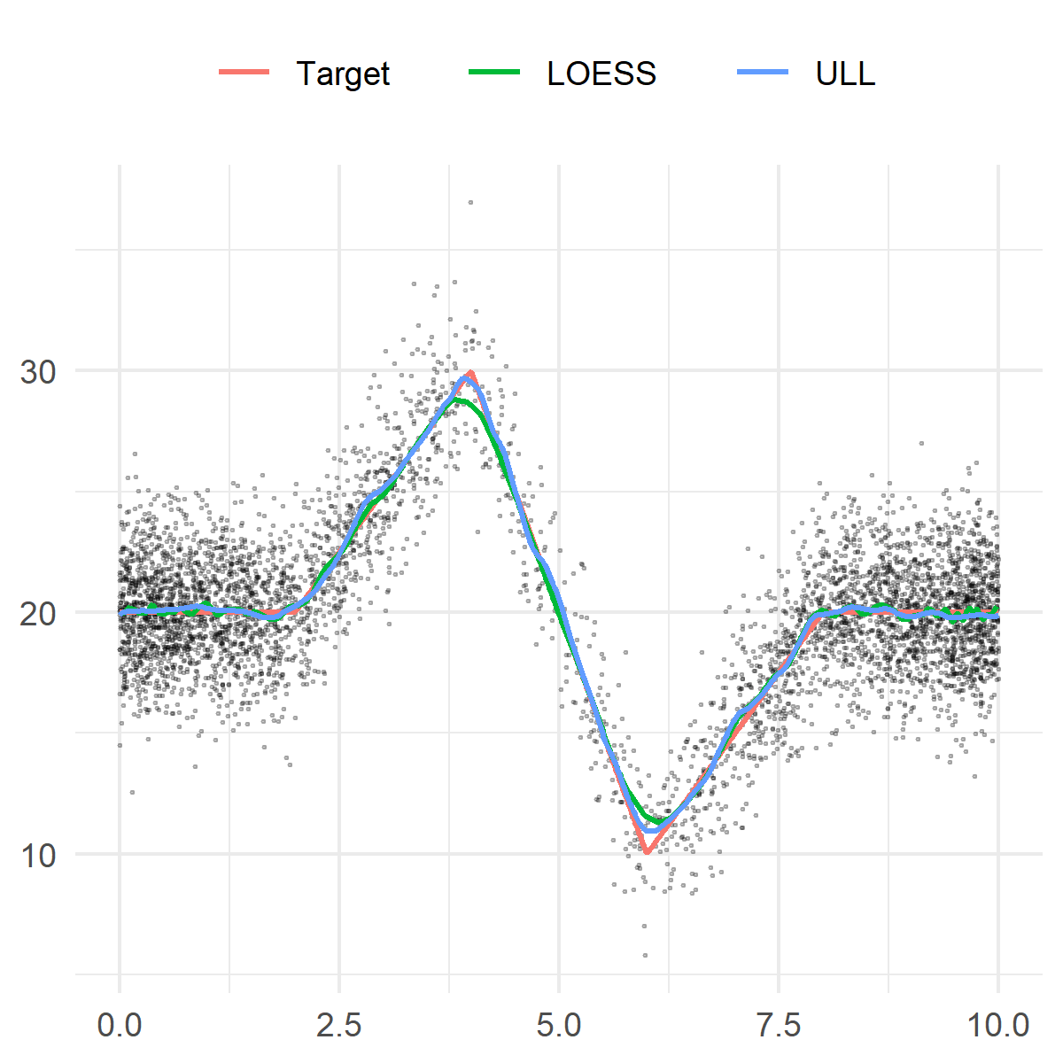
The piecewise linear target function is shown in Fig. 3. For the sake of simplicity of presentation, we do not present the formula for the definition of this function. Here the centered Gaussian noise has the standard deviation . The design points are independent and identically distributed with density proportional to the function , .


Example 4.
In this example, the design points are strongly dependent. We will define them as follows: , , where is a positive number such that is irrational (we chose in this example),
and are independent uniformly distributed on random variables independent of the noise. It was shown [4] that the random sequence is asymptotically everywhere dense on with probability 1.


Example 5.
In this example, the target function was the same as in Example 4. The difference from the previous example is that 50,000 design points were generated by the same technique, and then 5,000 points of the 50,000 ones were selected. This allowed us to fill the domain of with design elements “more uniformly” than in the previous example, while preserving the clusters of design points.

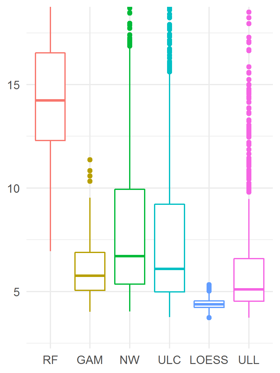
For maximum error, estimator (27) turns out to be the best of all the considered estimators. In particular, estimator (27) is better than LOESS: 2.872 (2.369, 3.488) vs. 9.435 (5.719, 10.9), .
For the mean squared error, the best estimator is LOESS. Estimator (27) is worse than LOESS: 5.108 (4.535, 6.597) vs. 4.378 (4.229, 4.541), , but it is better than the other estimators considered.
6 Example of processing real medical data
In this section, we consider an application of the models considered in the previous section to the data collected in the multicenter study “Epidemiology of cardiovascular diseases in the regions of the Russian Federation”. In that study, representative samples of unorganized male and female populations aged 25–64 years from 13 regions of the Russian Federation were studied. The study was approved by the Ethics Committees of the three federal centers: State Research Center for Preventive Medicine, Russian Cardiology Research and Production Complex, Almazov Federal Medical Research Center. Each participant has written informed consent for the study. The study was described in detail in [51].
One of the urgent problems of modern medicine is to study the relationship between heart rate (HR) and systolic arterial blood pressure (SBP), especially for low values of the observations. Therefore we will choose SBP as the outcome, and HR as the predictor. The association between these variables was previously estimated to be nonlinear [52]. The general analysis included 6597 participants from 4 regions of the Russian Federation. The levels of SBP and HR were statistically significantly pairwise different between the selected regions. Thus, the hypothesis of the independence of design points was violated.
In this section, the maximum error cannot be calculated because the exact form of the relationship is unknown, so only the mean squared error is reported. The mean squared error was calculated for 1000 random partitions of the entire set of observations into training () and validation () samples.

the results are presented in Fig. 8. Here the GAM estimator and the kernel estimators showed similar results, which were better than the results of both the linear regression and random forest.
The best estimator turned out to be (28), although its difference from the Nadaraya-Watson estimator was not statistically significant: 220.2 (215.4, 225.9) vs. 220.4 (215.4, 225.8), . The difference between estimator (27) and LOESS was not significant too: 220.4 (215.4, 225.9) vs. 220.6 (215.6, 226.1), .
7 Conclusion
In this paper, for a wide class of nonparametric regression models with a random design, universal uniformly consistent kernel estimators are proposed for an unknown random regression function of a scalar argument. These estimators belong to the class of local linear estimators. But in contrast to the vast majority of previously known results, traditional conditions of dependence of design elements are not needed for the consistency of the new estimators. The design can be either fixed and not necessarily regular, or random and not necessarily consisting of independent or weakly dependent random variables. With regard to design elements, the only condition that is required is the dense filling of the regression function domain with the design points.
Explicit upper bounds are found for the rate of uniform convergence in probability of the new estimators to an unknown random regression function. The only characteristic explicitly included in these estimators is the maximum spacing statistic of the variational series of design elements, which requires only the convergence to zero in probability of the maximum spacing as the sample size tends to infinity. The advantage of this condition over the classical ones is that it is insensitive to the forms of dependence of the design observations. Note that this condition is, in fact, necessary, since only when the design densely fills the regression function domain, it is possible to reconstruct the regression function with some accuracy. As a corollary of the main result, we obtain consistent estimators for the mean function of continuous random processes.
In the simulation examples of Section 5, the new estimators were compared with known kernel estimators. In some of the examples, the new estimators proved to be the most accurate. In the application to real medical data considered in Section 6, the accuracy of new estimators was also comparable with that of the best-known kernel estimators.
8 Proofs
In this Section, we will prove the assertions stated in Sections 2–4. Denote
| (32) |
Taking into account the relations , and the identity
| (33) |
we obtain the representation
| (34) |
where
We emphasize that, in view of the properties of the density , the domain of summation in the last two sums as well as in all sums defining the quantities from (4) coincides with the set , which is a crucial point for further analysis.
Lemma 1.
For , the following equalities are valid
| (35) | |||
| (36) |
Moreover, on the set of elementary events such that , the following inequalities hold
| (37) | |||
| (38) | |||
| (39) |
Proof. Let us prove (35) and (36). First of all, note that, due to the Cauchy–Bunyakovsky–Schwartz inequality, for all and this difference is continuous in . First, consider the simplest case where . For such , after changing the integration variable in the definition (21) of the quantities we have
| (40) |
i.e., , , and . In other words, on the segment , the following identity is valid
| (41) |
We now consider the case for all . Then
| (42) |
Next, by (42), we obtain
in view of the relation since is an even function. Similarly we study the symmetrical case where for all . ¿From here and (41) we obtain the first relation in (35):
The second relation in (35) directly follows from (42). Moreover, the above-mentioned arguments and the representations (40) and (42) imply (36).
Further, the first estimator in (37) is obvious by the above remark about the domain of summation in the definition of functions , and the relations
| (43) |
The second estimator in (37) immediately follows from the well-known estimate of the error of approximation by Riemann integral sums of the corresponding integrals of smooth functions on a finite closed interval:
| (44) |
where the functions , , are defined for all , and is the Lipschitz constant of the function ; It easy to verify that for all and . So, on the set of elementary events such that (recall that ), the right-hand side in (44) can be replaced with .
In addition, taking (36) and (37) into account, we obtain
Hence follows the estimate
| (45) |
The inequalities in (38) follow from (35), (45), and the definition of the constant .
Thus, Lemma 1 is proved.
Lemma 2.
For any positive , the following estimate is valid
Proof. Without loss of generality, the required estimate can be derived on the set of elementary events determined by the condition . Then the assertion of the lemma follows from the inequality
| (47) |
Lemma 3.
For any and , on the set of elementary events such that , the following estimate is valid
where the symbol denotes the conditionsl probability given the -field .
Proof. Put
| (48) |
where , and note that from Lemma 1 and the conditions of Lemma 3 it follows that, firstly, if only , and secondly,
| (49) |
The distribution tail of the random variable will be estimated by the so-called chaining proposed by A.N. Kolmogorov to estimate the distribution tail of the supremum norm of a stochastic process with almost surely continuous trajectories (see [9]). First of all, note that the set under the supremum sign can be replaced by the set of dyadic rational points
Thus,
where the natural number is defined by the equality (here is the minimal natural number greater than or equal to . One has
| (50) |
where is a sequence of positive numbers such that .
Let us now estimate each of the terms on the right-hand side of (8). Using Markov’s inequality for the second moment and the estimates (43), we obtain
| (51) |
Further,
| (52) |
Here we took into account that the summation range in (8) coincides with the set
and hence, due to the relation for , the estimate (46) is valid for and . Moreover, we used the estimates
and took into account the following inequalities in the above range of parameter changes (see Lemma 1):
We now obtain from (8)–(8) that
The optimal sequence minimizing the right-hand side of this inequality is and for , where is defined by the relation . For the indicated sequence, we conclude that
The assertion of the lemma follows from (49).
Proof of Theorem 1. The assertion follows from Lemmas 2 and 3 if we set
and take into account the relation
which was required.
To prove Theorem 2 we need the two auxiliary assertions below.
Lemma 4.
If the condition (16) is fulfilled then and for independent copies of the a.s. continuous random process the following strong law of large numbers is valid As , then
| (53) |
Proof. The first assertion of the lemma follows from (16) and Lebesgue’s dominated convergence theorem. We put
For any fixed and , one has
| (54) |
Put and note that , and as ,
Therefore, the right-hand side in (8) does not exceed and by the arbitrariness of and the first statement of the lemma, the relation (53) is proved.
Lemma 5.
Under the conditions of Theorem 2 the following limit relation holds
| (55) |
Proof. Let the sequences and be such that condition (17). Introduce the event , where . For any positive one has
| (56) |
Next, from Theorem 1 we obtain
To complete the proof of the lemma, it remains for the first probability on the right-hand side of (56) to apply Markov’s inequality, use the last estimate, limit relations (17), and the first statement of Lemma 4.
Proof of Proposition 2. For the estimator defined in (19), we need the following representation:
| (57) |
where
In view of the representations (34) and (57), we obtain
| (58) | |||
| (59) |
where . Further, it follows from Lemma 1 that, under the condition , for any point one has
| (60) |
When deriving the relation (60), we also took into account that and for all (see the proof of Lemma 1). Now, reckoning with the relations (43), (8), (8), (60), and Lemma 1, it easy to derive the first assertion of the lemma since
| (61) |
To prove the second assertion, first of all, note that
Thus, we need to compare the two variances on the right-hand side of the first equality with the corresponding variances of the second one. Using (43) and (60), we get
when deriving this estimate, we took into account that
To estimate the difference , note that the bound for the modulus of the difference between the squares of the displacements of the random variables and is essentially contained in (47) and (61). Estimation of the difference of the second moments of the specified random variables is done similarly with (43), (60), and (61):
which completes the proof.
Proof of Proposition 3. ¿From the definition of in (32) it follows that, for any ,
where . Expanding the function by the Taylor formula in a neighborhood of the point (up to the second derivative), from the above identities we obtain, using (32), (8), and lemma 1, that for any point we have
| (62) |
moreover, the - and -symbols on the right-hand side of (62) are uniform in . Note that holds for any .
Next, since for we have and for all natural , the following asymptotic representation holds:
| (63) |
Acknowledgments
Yu. Linke, I. Borisov, and P. Ruzankin were supported within the framework of the state contract of the Sobolev Institute of Mathematics, project FWNF-2022-0009.
References
- [1] Benelmadani, D.; Benhenni, K.; Louhichi, S. Trapezoidal rule and sampling designs for the nonparametric estimation of the regression function in models with correlated errors. Statistics. 2020, 54, 59–96; doi: 10.1080/02331888.2020.1715409.
- [2] Benhenni, K.; Hedli-Griche, S.; Rachdi, M. Estimation of the regression operator from functional fixed-design with correlated errors. J. Multivariate Anal. 2010, 101, 476–490; doi: 10.1016/j.jmva.2009.09.019.
- [3] Beran, J.; Feng, Y. Local polynomial estimation with a FARIMA-GARCH error process. Bernoulli. 2001, 7, 733–750; doi: 10.2307/3318539.
- [4] Borisov, I.S.; Linke, Yu.Yu.; Ruzankin, P.S. Universal weighted kernel-type estimators for some class of regression models. Metrika. 2021, 84, 141–166; doi: 10.1007/s00184-020-00768-0.
- [5] Cai, T.T.; Yuan, M. Optimal estimation of the mean function based on discretely sampled functional data: phase transition. Ann. Statist. 2011, 39, 5, 2330–2355; doi: 10.1214/11-AOS898.
- [6] Cao, G.; Wang, L.; Li, Y.; Yang, L. Oracle-efficient confidence envelopes for covariance functions in dense functional data. Statistica Sinica. 2016, 26, 359–383; doi: 10.5705/ss.2014.182.
- [7] Cao, G.; Yang, L.; Todem D. Simultaneous inference for the mean function of dense functional data. J. Nonparametr. Statist. 2012, 24, 359–377; doi: 10.1080/10485252.2011.638071.
- [8] Chen, J.; Gao, J.; Li, D. Estimation in semi-parametric regression with non-stationary regressors. Bernoulli. 2012, 18, 678–702; doi: 10.3150/10-BEJ344.
- [9] Chentsov, N. N. Weak convergence of stochastic processes whose trajectories have no discontinuities of the second kind and the heuristic approach to the Kolmogorov-Smirnov tests. Theory Probab. Appl. 1956, 1, 140–144; doi: 10.1137/1101013.
- [10] Chu, C. K.; Deng, W.-S. An interpolation method for adapting to sparse design in multivariate nonparametric regression. J. Statist. Plann. Inference. 2003, 116, 91–111; doi: 10.1016/S0378-3758(02)00184-2.
- [11] Chu, C.-K.; Marron, J. S. Choosing a Kernel Regression Estimator. Statistical Science. 1991, 6, 404–419; doi: 10.1214/ss/1177011586.
- [12] Devroye, L.P. The uniform convergence of the Nadaraya–Watson regression function estimate. Can. J. Stat. 1979, 6, 179–191; doi: 10.2307/3315046.
- [13] Einmahl, U.; Mason, D.M. Uniform in bandwidth consistency of kernel-type function estimators. Ann. Statist. 2005, 33, 1380–1403; doi: 10.1214/009053605000000129.
- [14] Fan, J.; Gijbels, I. Local polynomial modelling and its applications; London: Chapman and Hall, 1996.
- [15] Fan, J.; Yao, Q. Nonlinear time series nonparametric and parametric methods; Springer, 2003.
- [16] Gasser, T.; Engel, J. The choice of weghts in kernel regression estimation. Biometrica. 1990, 77, 277–381; doi: 10.1093/biomet/77.2.377.
- [17] Gu, W.; Roussas, G. G.; Tran, L. T. On the convergence rate of fixed design regression estimators for negatively associated random variables. Stat. Probab. Lett. 2007, 77, 1214–1224; doi: 10.1016/j.spl.2007.03.007.
- [18] Györfi, L.; Kohler, M.; Krzyzak, A.; Walk, H. A distribution-free theory of nonparametric regression; Springer, 2002.
- [19] Hall, P.; Müller, H.-G.; Wang, J.-L. Properties of principal component methods for functional and longitudinal data analysis. Ann. Statist. 2006, 34, 1493–1517; doi: 10.1214/009053606000000272.
- [20] Hansen, B.E. Uniform convergence rates for kernel estimation with dependent data. Econometric Theory. 2008, 24, 726–748; doi: 10.1017/S0266466608080304.
- [21] Härdle, W.; Luckhaus, S. Uniform consistency of a class of regression function estimators. Ann. Statist. 1984, 12, 612–623; doi: 10.1214/aos/1176346509.
- [22] Härdle, W. Applied nonparametric regression; Cambridge University Press, 1990.
- [23] Hastie, T.; Tibshirani, R.; Friedman, J. The elements of statistical learning: data mining; inference; and prediction; Springer New York, NY, 2009; doi: 10.1007/978-0-387-21606-5.
- [24] Hong, S. Y.; Linton, O. B. Asymptotic properties of a Nadaraya-Watson type estimator for regression functions of infinite order. 2016. cemmap working paper, No. CWP53/16, Centre for Microdata Methods and Practice (cemmap), London; doi: 10.1920/wp.cem.2016.5316.
- [25] Hsing, T.; Eubank, R. Theoretical Foundations of Functional Data Analysis; with an Introduction to Linear Operators; Wiley, 2015.
- [26] Ioannides, D. A. Consistent nonparametric regression: Some generalizations in the fixed design case J. Nonparametr. Stat. 1993, 2, 203–213; doi: 10.1080/10485259308832553.
- [27] Jiang, J.; Mack, Y.P. Robust local polynomial regression for dependent data. Statistica Sinica. 2001, 11, 705–722.
- [28] Karlsen, H.A.; Myklebust, T.; Tjøstheim D. Nonparametric estimation in a nonlinear cointegration type model. Ann. Statist. 2007, 35, 252–299; doi: 10.1214/009053606000001181.
- [29] Kokoszka, P.; Reimherr, M. Introduction to functional data analysis; Chapman and Hall/CRC, 2017.
- [30] Kulik, R.; Lorek, P. Some results on random design regression with long memory errors and predictors. J. Statist. Plann. Infer. 2011, 141, 508–523; doi: 10.1016/j.jspi.2010.06.030.
- [31] Li, Y.; Hsing, T. Uniform convergence rates for nonparametric regression and principal component analysis in functional/longitudinal data. Ann. Statist. 2010, 38, 3321–3351; doi: 10.1214/10-AOS813.
- [32] Liang, H.-Y.; Jing, B.-Y. Asymptotic properties for estimates of nonparametric regression models based on negatively associated sequences. J. Multivariate Anal. 2005, 95, 227–245; doi: 10.1016/j.jmva.2004.06.004.
- [33] Liero, H. Strong uniform consistency of nonparametric regression function estimates. Probab. Th. Rel. Fields. 1989, 82, 587–614; doi: 10.1007/BF00341285.
- [34] Li, X; Yang, W.; Hu, S. Uniform convergence of estimator for nonparametric regression with dependent data. J. Inequal. Appl. 2016, 142 (2016); doi: 10.1186/s13660-016-1087-z.
- [35] Lin, Z.; Wang, J.-L. Mean and Covariance Estimation for Functional Snippets. J. Amer. Statist. Assoc. 2020, 117, 1–39; doi: 10.1080/01621459.2020.1777138.
- [36] Linke, Yu.Yu. Asymptotic properties of one-step M-estimators. Communications in Statistics: Theory and Methods. 2019, 48, 4096–4118; doi: 10.1080/03610926.2018.1487982.
- [37] Linke, Yu.Yu. Towards insensitivity of Nadaraya–Watson estimators to design correlation. Theory Probab. Appl. 2022, 67 (to appear)
- [38] Linke, Yu.Yu.; Borisov, I.S. Constructing explicit estimators in nonlinear regression problems. Theory Probab. Appl. 2018, 63, 22–44; doi: 10.1137/S0040585X97T988897.
- [39] Linke, Yu.Yu.; Borisov, I.S. Constructing initial estimators in one-step estimation procedures of nonlinear regression. Statist. Probab. Lett. 2017, 120, 87–94; doi: 10.1016/j.spl.2016.09.022.
- [40] Linke, Yu.Yu.; Borisov, I.S. Insensitivity of Nadaraya–Watson estimators to design correlation. Communications in Statistics: Theory and Methods. 2021; doi: 10.1080/03610926.2021.1876884.
- [41] Linton, O. B.; Jacho-Chavez, D. T. On internally corrected and symmetrized kernel estimators for nonparametric regression. TEST. 2010, 19, 166–186; doi: 10.1007/s11749-009-0145-y.
- [42] Linton, O.; Wang, Q. Nonparametric transformation regression with nonstationary data. Econometric Theory. 2016, 32, 1–29; doi: 10.1017/S026646661400070X.
- [43] Mack, Y.P.; Silvermann, B.W. Weak and strong uniform consistency of kernel regression estimates. Z. Wahrscheinlichkeitstheor. Verw. Geb. 1982, 61, 405–415; doi: 10.1007/BF00539840.
- [44] Masry, E. Nonparametric regression estimation for dependent functional data. Stoch. Proc. Their Appl. 2005, 115, 155–177; doi: 10.1016/j.spa.2004.07.006.
- [45] Müller, H.-G. Density adjusted kernel smoothers for random design nonparametric regression. Stat. Probab. Lett. 1997, 36, 161–172; doi: 10.1016/S0167-7152(97)00059-X.
- [46] Müller, H.-G. Functional modelling and classification of longitudinal data. Scand. J. Statist. 2005, 32, 223–246; doi: 10.1111/j.1467-9469.2005.00429.x.
- [47] Müller, H.-G. emphNonparametric regression analysis of longitudinal Data; New York: Springer, 1988.
- [48] Nadaraya, E. A. Remarks on non-parametric estimates for density functions and regression curves. Theory Prob. Applications. 1970, 15, 134–137; doi: 10.1137/1115015.
- [49] Rio, E. Moment Inequalities for Sums of Dependent Random Variables under Projective Conditions. J. Theor. Probab. 2009, 22, 146–163; doi: 10.1007/s10959-008-0155-9.
- [50] Roussas, G.G. Nonparametric regression estimation under mixing conditions. Stoch. Proc. Appl. 1990, 36, 107–116; doi: 10.1016/0304-4149(90)90045-T.
- [51] Shalnova, S.A.; Drapkina, O.M. Significance of the ESSE-RF study for the development of prevention in Russia. (In Russian) Cardiovascular therapy and prevention. 2020, 19, 2602; doi: 10.15829/1728-8800-2020-2602.
- [52] Shalnova, S.A.; Kutsenko, V.A.; Kapustina, A.V.; Yarovaya, E.B.; et al. Associations of Blood Pressure and Heart Rate and Their Contribution to the Development of Cardiovascular Complications and All-Cause Mortality in the Russian Population of 25-64 Years. (In Russian) Rational Pharmacotherapy in Cardiology. 2020, 16, 759–769; doi: 10.20996/1819-6446-2020-10-02.
- [53] Shen, J.; Xie, Y. Strong consistency of the internal estimator of nonparametric regression with dependent data. Stat. Probab. Lett. 2013, 83, 1915–1925; doi: 10.1016/j.spl.2013.04.027.
- [54] Tang, X.; Xi, M.; Wu, Y.; Wang, X. Asymptotic normality of a wavelet estimator for asymptotically negatively associated errors. Stat. Probab. Lett. 2018, 140, 191–201; doi: 10.1016/j.spl.2018.04.024.
- [55] Wang, Q.; Chan, N. Uniform convergence rates for a class of martingales with application in non-linear cointegrating regression. Bernoulli. 2014, 20, 207–230; doi: 10.3150/12-BEJ482.
- [56] Wang, J.-L.; Chiou, J.-M.; M’́uller, H.-G. Functional Data Analysis. Annu. Rev. Statist. 2016, 3, 257–295; doi: 10.1146/annurev-statistics-041715-033624
- [57] Wu, J.S.; Chu, C.K. Nonparametric estimation of a regression function with dependent observations. Stoch. Proc. Their Appl. 1994, 50, 149–160; doi: 10.1016/0304-4149(94)90153-8.
- [58] Wu, H.; Zhang, J.-T. Nonparametric regression methods for longitudinal data analysis: mixed-effects modeling approaches; John Wiley and Sons, 2006.
- [59] Yao, F. Asymptotic distributions of nonparametric regression estimators for longitudinal or functional data. J. Multivariate Anal. 2007, 98, 40–56; doi: 10.1016/j.jmva.2006.08.007.
- [60] Yao, F.; M’́uller, H.-G.; Wang, J.-L. Functional data analysis for sparse longitudinal data. J. Amer. Statist. Assoc. 2005, 100, 577–590; doi: 10.1198/016214504000001745.
- [61] Zhang, J.-T.; Chen, J. Statistical inferences for functional data. Ann. Statist. 2007, 35, 1052–1079; doi: 10.1214/009053606000001505.
- [62] Zhang, X.; Wang, J.-L. From sparse to dense functional data and beyond. Ann. Statist. 2016, 44, 2281–2321; doi: 10.1214/16-AOS1446.
- [63] Zheng, S.; Yang, L.; Hardle, W. A smooth simultaneous confidence corridor for the mean of sparse functional data. J. Amer. Statist. Assoc. 2014, 109, 661–673; doi: 10.1080/01621459.2013.866899.
- [64] Zhou, L.; Lin, H.; Liang, H. Efficient estimation of the nonparametric mean and covariance functions for longitudinal and sparse functional data. J. Amer. Statist. Assoc. 2018, 113, 1550–1564; doi: 10.1080/01621459.2017.1356317.
- [65] Zhou, X.; Zhu, F. Asymptotics for L1-wavelet method for nonparametric regression. J. Inequal. Appl. 2020, 216 (2020); doi: 10.1186/s13660-020-02483-w.