A necessary condition for Sobolev extension domains in higher dimensions
Abstract.
We give a necessary condition for a domain to have a bounded extension operator from to for the range . The condition is given in terms of a power of the distance to the boundary of integrated along the measure theoretic boundary of a set of locally finite perimeter and its extension. This generalizes a characterizing curve condition for planar simply connected domains, and a condition for -extensions. We use the necessary condition to give a quantitative version of the curve condition. We also construct an example of an extension domain that is homeomorphic to a ball and has -dimensional boundary.
Key words and phrases:
Sobolev extension2000 Mathematics Subject Classification
Primary 46E35.1. Introduction
A domain is called a -extension domain, if we can extend each Sobolev function to a global Sobolev function so that the Sobolev norm of the extension is at most a constant times the norm of the original function. Sobolev extension domains are interesting in several fields of analysis because on those one can use many functional-analytic tools that are classically available for functions defined on the whole space. Examples of Sobolev-extension domains include Lipschitz domains [5, 32] and more generally, -domains [18]. For our context, the Lipschitz and results should be seen as sufficient conditions on the boundary of the domain for the extendability of Sobolev functions. In this paper, we continue investigating the converse direction by finding a new necessary condition for extendability.
Several necessary geometric conditions on the boundary of Sobolev extension domains are already known. For instance, all Sobolev extension domains have positive densities at all the points belonging to them (this is usually referred as to satisfy a measure density condition, [19, 15]). Then, by the Lebesgue differentiation theorem we must have that their boundaries are of zero Lebesgue measure. In general we cannot improve this to a non-trivial dimension upper bound on the boundary of a Sobolev extension domain: take for example with a Cantor set with zero Lebesgue measure and so that .
However, one can still meaningfully study the dimension of the boundary of extension domains. One approach is to limit the topology or other properties of the domain, and another one is to investigate only those points that are more relevant for the extendability. The second approach leads to the study of the size of the set of two-sided points of the boundaries of Sobolev extension domains (that is, points where the boundary might self-intersect and hence can be approached from two different sides in the domain). In the case we have that -extension domains are quasiconvex (see [19, Theorem 3.1]) and then the set of two-sided points must be empty. The case is more interesting and has been investigated in [33, 10], where bounds on the Hausdorff dimension of the set of two-sided points are found.
Non-trivial dimension upper bounds for the whole boundary have been obtained only in the special case of planar bounded simply connected extension domains [25]. These bounds are based on the porosity of the boundary that is implied by the geometric characterizations of bounded simply connected planar Sobolev extension domains, see (1.1) and (1.2) below. The first such characterizations established that a bounded simply connected domain is a -extension domain if and only if is a quasidisk (see [11, 12, 13, 18]).
In the case , Shvartsman [30] proved that a bounded finitely connected domain is a -extension domain if and only if for some the following condition is satisfied: for every there exists a rectifiable curve joining and so that
| (1.1) |
Let us mention that in [31], the curve condition (1.1) was also shown to characterize -extension domains for every and . Here we define the homogeneous Sobolev space to be the space of locally integrable functions whose distributional partial derivatives belong to .
Finally, for the case the following result is proved in [22]: a bounded simply connected domain is a -extension domain if and only if there exists such that for every there exists a curve connecting and such that
| (1.2) |
In Theorem 1.1 we generalize the condition (1.2) to higher dimensions; still for the range of exponents. Before stating our result, let us look at the limiting case that partly motivates our formulation.
In the case of a bounded simply connected planar domain , by the results from [23], we know that is a -extension domain if and only if for every there exists a curve connecting and with
| (1.3) |
In other words, the correct limit of the term in (1.2) is as . The characterizing property (1.3) can also be seen as a combination of earlier results on -extension domains and the following more general planar result [9]: A bounded -extension domain is a -extension domain if and only if the -dimensional measure of the set
intersected with any Lipschitz curve is zero, where are the connected components of . Recall that the space consists of integrable functions whose total variation
is finite. As observed in [9], the above characterization of -extension domains holds only in the plane. This is essentially because the planar topology allows one to write the essential boundary of a set of finite perimeter as the union of Jordan loops, see [1, Corollary 1] (recalled in Proposition 2.2 below).
In higher dimension where such decomposition result does not hold, the characterization is written in terms of sets of finite perimeter. Before going to this characterization, let us recall an earlier result on -extension domains, where
In [4], Burago and Maz’ya proved the following characterization of -extension domains: is a -extension domain if and only if there exists some constant so that any set of finite perimeter in admits an extension satisfying and
Since -extension domains are known to be -extension domains (the proof of this fact follows the same ideas as one may find in [21, Lemma 2.4]), the above property about extension of sets of finite perimeter is a necessary condition both for - and -extension domains.
In order to turn this into a characterization of - or -extension domains, we have to account for the intersection of the boundary of the extended set with the boundary of the domain, analogously to (1.3). This leads to the following characterization in terms of strong extension of sets of finite perimeter [9]: A bounded domain is a -extension domain if and only if any set of finite perimeter in admits an extension satisfying ,
where denotes the measure theoretic boundary of . In order to remind ourselves of the analogous condition in the planar simply connected case as the limit of (1.2), we can rewrite this in an integral form
This motivates the formulation of the following main theorem of this paper.
Theorem 1.1.
Let be an -extension domain for some . Then for any and any measurable set there exists a set with and
| (1.4) |
where denotes the norm of the -extension operator, and the constant depends only on , and .
Let us immediately comment on the range of exponents and the use of the homogeneous Sobolev space in Theorem 1.1. The reason for the range of exponents is that if , then the integral on the right-hand side of (1.4) is infinite for any set for which the zero-extension would not satisfy (1.4). Thus, for the conclusion of Theorem 1.1 provides no information.
The use of the homogeneous Sobolev space is natural for scaling invariant results. In the case is bounded, the result still applies for -extension domains because these are known to be -extension domains as well (see [19]). When thinking about moving between - and -extensions in bounded domains, one should observe that for a set occupying most of (in our proof, for satisfying ) the extension satisfying (1.4) has to contain all of the space that is sufficiently far away from .
It is worth noticing also that, if is bounded, any measurable set for which the right hand side of the inequality (1.4) is finite must be of finite perimeter in , and also the set that we construct will be of finite perimeter in . If were unbounded we would only have that and are locally of finite perimeter in and in , respectively.
One might wonder if the condition in Theorem 1.1 is also sufficient for to be an -extension domain. It turns out that this is not the case: Suppose is an arbitrary domain. We can modify to a new domain , where the balls are selected in such a way that (giving that we have an extension operator from to ), but so that they accumulate densely enough to the boundary of so that for any with the right-hand side of (1.4) finite for , the extension can be taken to be zero outside so that the condition (1.4) again gives us no information on .
In dimensions at least three, one can make the above idea into a construction of a topologically nice extension domain with large boundary. In the version of the construction that we use to prove the following theorem, the removed balls from the domain are replaced by removed tubes, and they accumulate only to a large portion of the boundary instead of the whole boundary.
Theorem 1.2.
There exists a domain such that for a homeomorphism , and is a -extension domain for all .
Note that the domain in Theorem 1.2 cannot be an -domain, nor a John domain, since these domains have porous boundaries and hence their Hausdorff (and packing) dimensions would be strictly less than three. We also reiterate that the same type of example is not possible in by the dimension bounds on the boundary of a simply connected planar Sobolev extension domain given in [25].
We wrote the dependence on the norm of the extension operator explicitly in Theorem 1.1 mainly in order to start the investigation of the dependence between the norm and the constant in (1.2). Using this explicit form, we obtain a more quantified version of the necessity of (1.2).
Theorem 1.3.
Let a bounded simply connected -extension domain for some . Then for every there exists a constant such that for all there exists a curve joining and so that
| (1.5) |
We do not claim nor expect the dependence on in (1.5) to be sharp. However, our proof of Theorem 1.3 written in Section 4 gives the first explicit dependence. Since (1.2) is a characterization, one could also try to get the dependence of the operator norm on the curve condition constant . This direction of the proof of the characterization in [22] is more technical. Consequently, we suspect the quantitative dependence in this direction to be more difficult to obtain.
Acknowledgements
The authors acknowledge the support from the Academy of Finland, grant no. 314789. This work was partly done while the first-named author was enjoying a postdoctoral position at the Department of Mathematics and Statistics of the University of Jyväkylä. He also wants to thank the department for their kind hospitality during his time there.
2. Preliminaries
In what follows, we use the notation to mean a strictly positive and finite function on the parameters listed in the parentheses, i.e. a constant once the listed parameters are fixed. The function (constant) may change between appearances even within a chain of inequalities.
For any point and radius we denote the open ball by More generally, for a set we define the open -neighbourhood as
We denote by the -dimensional outer Lebesgue measure of a set . For any Lebesgue measurable subsets and any point we define the upper density of at over as
and the lower density of at over as
If , we call the common value the density of at over and denote it by . If we simply write , and . The essential interior of is then defined as
the essential closure of as
and the essential boundary of as
As usual, stands for the -dimensional Hausdorff measure of a set obtained as the limit
where is the -dimensional Hausdorff -content of defined as
By a dyadic cube we refer to for some and . We denote the side-length of such dyadic cube by .
2.1. Sets of finite perimeter
A Lebesgue measurable subset has finite perimeter in an open set if , where denotes the characteristic function of the set . We set and call it the perimeter of in . Here
denotes the total variation of on .
It is well known that a set has finite perimeter in if and only if (see [8, Section 4..5.11]). Let us recall as well the isoperimetric inequality, which follows from the -Poincaré inequality for functions (see for instance [2, Theorem 3.44]).
Proposition 2.1.
Let be an open set and a set of finite perimeter in . Let also be two dyadic cubes with and so that is connected. Then we have
| (2.1) |
Moreover, for every and ,
| (2.2) |
The study of the boundary of sets of finite perimeter can be reduced to the study of Jordan loops via the following decomposition result from [1, Corollary 1].
Proposition 2.2.
Let have finite perimeter. Then, there exists a unique decomposition of into rectifiable Jordan curves , modulo -measure zero sets, such that
- (1)
Given , , they are either disjoint or one is contained in the other; given , , , they are either disjoint or one is contained in the other. Each is contained in one of the .
- (2)
.
- (3)
If , , then there is some rectifiable Jordan curve such that . Similarly, if , , then there is some rectifiable Jordan curve such that .
- (4)
Setting , the sets are pairwise disjoint, indecomposable and
2.2. Whitney decomposition
If is an open set, not equal to the entire space , we let be the standard Whitney decomposition of , by which we mean that it satisfies the following properties:
- (W1)
Each is a closed dyadic cube inside .
- (W2)
and for every we have .
- (W3)
For every we have ,
- (W4)
If , we have .
The reader can find a proof of the existence of such a dyadic decomposition of the set in [32, Chapter VI].
For such Whitney decomposition we take a partition of unity so that for every we have , , , , and
Notice that for each the above together with the bound on the size of the supports and (W4) implies
| (2.3) |
In order to ease the notation, we denote for each by the collection of neighboring cubes that have a common face with :
2.3. Size estimates
In this subsection we recall the remaining key auxiliary results that will be used in the paper.
The following lemma is a modification of [22, Lemma 3.2]. This version of the estimate was proven in [10, Lemma 2.3]. (Here we can simplify the presentation a bit since we do not need an exceptional set .)
Proposition 2.3.
Let be an -dimensional cube in with sides parallel to the coordinate axes. Let for some and suppose there exists so that
Then
For -extension domains with the following measure density condition holds for points . This version of the measure density condition was proven in [10, Proposition 2.2] following the results in [15], see also [19].
Proposition 2.4.
Let and let be a Sobolev -extension domain with an extension operator . Then, for all and
we have
3. Proof of the necessary condition
In this section we prove Theorem 1.1. In order to make the structure of the proof clearer, we first present the proof assuming the more technical parts proven. These technical parts are stated as separate lemmata. They are then proven after the proof of Theorem 1.1.
Proof of Theorem 1.1.
We start with a measurable set so that
| (3.1) |
Notice that if (3.1) fails, we can simply take as the set satisfying the required inequality (1.4).
Following the definitions in Subsection 2.2, let and be the Whitney decompositions of and respectively, and let be the partition of unity in subordinate to .
We first modify our set by means of selecting those Whitney cubes that intersect the set in a large enough measure set. Namely, we let
It will be easier to handle this new set rather than the original set .
Next, for the constant we define
Our extension of the set is then defined as
The task in proving Theorem 1.1 is now to show that the choice of above works. We divide this task into several lemmata. The first lemma justifies the replacement of by .
Lemma 3.1.
For the sets and above we have
The next step is then to go from the set to a Sobolev function to which we can apply our -extension operator. This is done with a Whitney smoothing operator defined via the partition of unity for . We define for any a smoothened version of as
| (3.2) |
Whitney smoothing operators similar to the one above have been used for instance in [14, 3, 24, 9].
In addition to smoothing the function, the operator has the important property of leaving the trace of the function unmodified on the boundary of . Within our proof, this is the content of the last Lemma 3.4. The second lemma relates the integral in (1.4) to the -norm of the gradient of the smoothened version of the indicator function. We write the lemma for a general set , but here inside the proof of Theorem 1.1 use it only for the set .
Lemma 3.2.
We now use to pass from the characteristic function to a Sobolev function
Lemma 3.2 together with Lemma 3.1 then gives us
| (3.3) |
The third lemma shows that the extension of the set has the correct property outside the closure of the domain . The fact that is a Sobolev-extension domain is used in the proof of this lemma. Recall that denotes the norm of the -extension operator.
Lemma 3.3.
With the and defined above, for every we have
The last lemma deals with the boundary of , where in principle some part of the measure theoretic boundary of could live and cause the integral on the left-hand side of (1.4) to be infinite.
Lemma 3.4.
With our set defined above, we have .
Let us then focus on proving the lemmata we used in the proof of Theorem 1.1.
Proof of Lemma 3.1.
Setting we start by writing
and
Hence, we only need to check that for with and we have . Assuming without loss of generality that and , this is seen by using the isoperimetric inequality (2.1)
Proof of Lemma 3.2.
From the definition of , for every we get
where
Assume that we have with . We may further assume that . Then, by using the isoperimetric inequality (2.1) we get
Hence, we have
Therefore, by using the finite overlapping between Whitney cubes, we have
Proof of Lemma 3.3.
We introduce the following subfamily of Whitney cubes of
We then have
Let us fix for the moment. Then there exists a neighbouring cube , that is , so that . By the definition of , we have
| (3.5) |
and
| (3.6) |
In particular, (3.5) and (3.6) imply that
Therefore,
| (3.7) |
Combining (3.7),(3.6) and (3.5) with the measure density condition stated in Proposition 2.4, we get
Recall that where . By (2.3) we have on and so if , then on and if , then on . Therefore,
Let . Then by Proposition 2.3, we have
This concludes our estimate for the fixed .
Now, since , we may use the boundedness of the Hardy-Littlewood maximal operator
to get
Since we may choose to be arbitrarily close to with the price of enlarging the constant , the lemma is proven. ∎
Proof of Lemma 3.4.
We divide the proof into three parts. The parts 1 and 3 will imply the claim of the lemma, while part 2 is needed in the proof of part 3.
Part 1: For -a.e. the limit exists and is either or .
Proof of Part 1.
Let
and assume towards contradiction that . Then, there exists so that for
Fix and for every choose so that , then
and hence by the Vitali covering theorem (see [6, Theorem 1.24]) there exists a countable collection so that
| (3.8) |
and . Recall that , and that by Lemma 3.2 and Lemma 3.1 we have
So, we have . We extend to . Observe that for every , by (3.8) and by the measure density condition (Proposition 2.4) we have
and
Therefore, by the definition of via , and the fact that is the union of the same Whitney cubes used in the definition of , we have
and
Hence, we may apply Proposition 2.3 to get the estimate
We can now conclude
Using that by the measure density condition , the right hand side tends to zero as . So which is a contradiction. We have thus proven Part 1. ∎
Part 2: The following two implications hold for -almost every :
| (3.9) |
and
| (3.10) |
Proof of Part 2.
Let us first show that by going to complements, we only need to prove (3.9). Towards this, assume that (3.9) is true for every measurable set . Suppose then that . Call and consider the associated
We have . Since , we have by assumption that . Thus, and we have shown (3.10). (Notice that the form of the definitions of the sets and differ slightly in that one has a strict inequality while the other does not. However, it is easy to observe that this does not affect the proof below.)
Let us then prove (3.9). The argument is similar to the proof of Part 1. This time we write
and assume towards contradiction that . Then, as in the previous proof, there exists so that for
Now, at this stage it is enough to notice that by the definition of we have
so that by the measure density, we have that for some
Now, repeating the proof of Part 1 gives the needed contradiction and proves (3.9) and thus Part 2. ∎
Part 3: The following two implications hold for -almost every :
| (3.11) |
and
| (3.12) |
Proof of Part 3.
Since the definition of passes (up to the difference between a strict and non-strict inequality) to the complements, similarly to the Part 2 it is enough to prove the implication (3.11).
Let with and . (Notice that by Part of the proof, this holds for -almost every with .) Now, if with , by the definition of and the measure density condition (Proposition 2.4) we have
| (3.13) |
Consider the collection
and let be the center of each . By the Vitali covering theorem there exists a subcollection so that
and
| (3.14) |
for any two with . Notice that (3.14) implies that also
Hence, by (3.13)
| (3.15) |
where is a constant depending only on so that for any with .
We can now conclude the proof of the lemma by taking for which the conclusions of Part 1 and Part 3 above hold. Part 1 of the proof says that exists and is either or . Then by Part 3 of the proof
and hence . ∎
4. A quantitative version of the curve condition
In the present section we use Theorem 1.1 to prove Theorem 1.3. This gives a quantitative version of a result proven in [22].
Theorem 1.3 states that if is a bounded simply connected -extension domain for some with an extension operator , then for every there exists a constant such that for all there exists a curve joining and so that
| (4.1) |
The curve condition (4.1) was proven in [22] to be a characterization of planar bounded simply connected -extension domains for (a similar characterizing condition for the complement of a bounded finitely connected planar domain for was given in [30]). Here we only prove the necessity, but provide a more explicit estimate on the dependence of the operator norm in (4.1).
The proof in [22] of the necessity of (4.1) starts by observing that the domain is -John, by results in [19, Theorem 6.4], [12, Theorem 3.4], and [29, Theorem 4.5]. Recall that a bounded domain is called -John for some constant if there is a point and a constant so that given we can find a curve parameterized by arc length joining with so that
| (4.2) |
The proof in [22] then continues by making a test function in and by constructing the required curve using conformal maps. These steps make it difficult to track the constants.
The proof of (4.1) in our approach starts by examining two conditions similar to the John condition. We first prove a quantitative version of the so-called condition (4.3) (see [29] for this and similar conditions) for Sobolev extension domains. In the lemma below and elsewhere in this section, for an injective curve (possibly defined on an open or half-open interval) and two points we denote by a minimal subcurve of so that is connected.
Lemma 4.1.
Let be a bounded simply connected -extension domain for some . Then for every there exists an injective curve connecting to and satisfying
| (4.3) |
for all , where .
Proof.
Let us first prove the claim for . By the Riemann mapping theorem there exists a conformal map . Since we know that is a John domain, by [29, Theorem 2.18] the domain is finitely connected along its boundary and hence extends as a continuous map to the boundary. We refer to this extension still by . Consider and so that one of the open arcs in connecting and does not intersect . Call this arc and write .
Using the sets and we now define a set
where the distance for a connected set and a point is defined by
Notice that since is a John domain we have for any non-empty arc and any that . This can be seen by taking , a sequence converging to , the John curves connecting to the John-center , and finally a subsequence of converging to the desired giving . The passage to an arbitrary follows since any two points inside can be connected by a curve in of finite length. Notice moreover, that is a continuous function.
We claim that is a closed set in so that and are in the same connected component of . Suppose this is not the case. Then there exists a path from to that does not intersect . However, the function
is continuous in , and so in particular along the path . Since is negative near and positive near the function must be zero on some point of . This contradicts and the claim is proven. Let us call the connected component of that contains the points and .
Now, consider the following open neighbourhood of
Since contains a connected component connecting to , we can find an injective curve so that is connected. Notice that at this point we do not know if can be extended to and as a curve connecting and , but after establishing (4.4) below, we have that the image curve extends uniquely to a curve defined on connecting to .
Next we will show that for any we have
| (4.4) |
Towards proving (4.4), let and be so that
| (4.5) |
The estimate (4.4) is shown if we can prove that necessarily . We may assume that .
Let be an injective curve in joining to and let be an injective curve in joining to so that they satisfy
Let be such that is a singleton. Now, the set has two connected components and so that and , or with and swapped. Consequently, by (4.5) the sets satisfy
Denote and notice that since , we have
| (4.6) |
Define the test function
Clearly and . Notice, that on and by (4.6) we have . Hence, for each there exists such that in . Thus, .
For the test function we have
Let be the extension operator. Then in polar coordinates
| (4.7) |
By absolute continuity and Hölder’s inequality for we have
Hence
| (4.8) |
By combining (4.7) and (4.8) we get
This gives the upper bound
| (4.9) |
Thus we have established (4.4) and the lemma is proven in the special case .
Let us then consider the general case . In this case we repeat the previous construction but replace by the simply connected domain where satisfy
and and denote the line segments from to and from to , respectively. Notice that is not necessarily a Sobolev extension domain. However, for points near and the condition (4.4) is satisfied trivially, and for points far from them, an enlarged ball meets the sets and , so one can still use the argument from the special case. ∎
The next step is to go from the condition (4.3) to a condition (4.10). Before stating this as a lemma, let us recall the corresponding implication from [26, p. 385–386] from the so-called condition to the so-called condition. This latter condition is very close to the John condition (4.2), where one of the endpoints of all the curves is a fixed point .
Lemma 4.2.
Let be a bounded domain and let . Suppose that there exists a curve such that for every
Then there exists another arc length parametrized curve with , and
Lemma 4.3.
Let be a bounded simply connected domain satisfying the condition (4.3) with some constant . Then for every there exists an injective curve connecting to and satisfying
| (4.10) |
for all , where .
Proof.
Let us first consider the case where . Let be a curve joining and and satisfying (4.3). Let be a point such that . Then, by using Lemma 4.2 separately to the curves and there exist arc length parameterized curves , for so that , , , and
The concatenation of and now gives the curve satisfying (4.10).
Consider then the general case . Let be sequences converging to the points and , respectively, and let be a collection of constant speed parametrized curves connecting to , and satisfying (4.10) with the same constant . Since is bounded and the lengths of the curves are uniformly bounded, by Arzelá-Ascoli there exists a sequence and a curve such that uniformly. Moreover, by the lower semicontinuity of length
for all . This concludes the general case.
We are now ready to prove the main result of this section.
Proof of Theorem 1.3.
Let , and a bounded and simply connected -extension domain. Let , , , and denote by the connected components of for which . We divide the proof into two steps.
Step 1: Let us first show that we can connect any points with a suitable curve. By Lemmata 4.1 and 4.3 we know that there exists a curve parametrized by arc length between and so that
| (4.11) |
for every , where
| (4.12) |
Let us denote by , , the subcurves of such that and . We parametrize so that . We consider two cases. Assume first that . By the condition (4.11) we have
Let us then consider the case . Let be the connected component of with and let be a cross-cut in connecting to a point in . Let be the first point where intersects when travelling from . Denote by the maximal arc containing such that . Let be the endpoints of . By reordering if necessary, there exist minimal times such that and . Let be the curve parametrizing by arc length. By (4.11), we have
for all . Suppose and satisfy . Then, since is contained in the interior of and , we have that the line segment intersects one of the at some point . Since , we have
Consequently,
Therefore (setting in the first case),
| (4.13) |
Finally, a connected component of has finite perimeter in , and since is bounded, the extension provided by Theorem 1.1 also has finite perimeter in . By Proposition 2.2, the boundary decomposes into Jordan loops .
There exists one Jordan curve in the decomposition with because the points must be in the same connected component of . We now write as a union of two curves, both having end points . Therefore and by Theorem 1.1 and (4.13), we have
| (4.14) |
Step 2: We now construct the curve by connecting the sets by suitable line-segments and by using Step 1 for each to connect the entrance and exit points of . See Figure 1 for an illustration of the construction of .

Let us first check that by (4.11), we get an upper bound for the number of sets . By the definition of sets , for all , so, there exists a curve in satisfying (4.11) that starts in and exits at some point so that
Consequently, there exists an arc such that . Hence, , and so
| (4.15) |
Let us then construct a curve connecting and such that (4.1) holds. For notational convenience, write and .
Define , and a continuous function by
Let , and
Denote by . By the selection of and we have , and there exists such that is connected.
We continue by induction. Suppose we have found , , and . Replacing with and with we repeat the above process until .
The above process gives us a (relabeled) sequence such that each adjacent pair , may be connected with where , , and and for the other indices, so that
| (4.16) |
For each we can connect and with a curve given by the special case that satisfies (4.14) with the obvious changes of notation.
5. A Sobolev extension domain with large boundary
In this section we prove Theorem 1.2 which states the existence of a domain such that for a homeomorphism , and is a -extension domain for all .
We define first the following Cantor set : Choose any strictly increasing sequence of positive numbers satisfying
For instance let . Define inductively a family of closed sets , with , so that each consists of disjoint cubes of sides , in such a way that for each , is formed by cubes equally distributed inside (denote ). Namely, they are at least at a distance between themselves and also from the boundary of .
Letting , we get a Cantor set of Hausdorff dimension but . The fact that follows from , while is implied by . We refer to [28, Corollary 4] for further details.
Let us next define tubes that approach our Cantor set. The tubes will be removed from the open unit cube to form so that . Define first to be the middle point of the upper face of a cube . Given a cube we denote by the larger cube that contains it from the previous iteration. Define a decreasing sequence of positive constants by setting and for all . In particular, we then have and for every .
The tubes will be defined as tubular neighbourhoods of curves joining a point on the top face of . We require the curves and points to satisfy the following conditions:
- (L1)
.
- (L2)
.
- (L3)
for .
- (L4)
The curves consist of segments that are parallel to the coordinate axes and have length at least .
- (L5)
approaches and perpendicular to the faces of and , respectively.
Using the curves we then define the tubes as
Next we define
for every , and finally our domain as
See Figure 2 for a two-dimensional illustration of the construction.
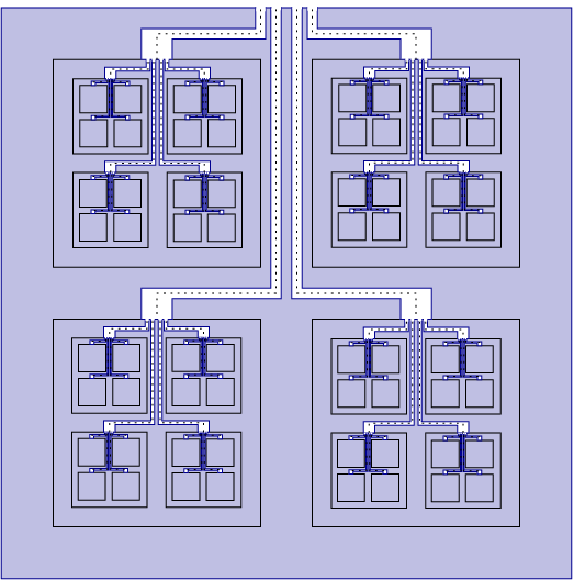
By construction, we have
Therefore, and as required. What remains to be checked is that is homeomorphic to the open unit ball and that it is a Sobolev -extension domain for all . We prove these separately in the following two lemmata.
Lemma 5.1.
There exists a homemorphism so that .
Proof.
It is enough to prove the existence of a homeomorphism so that since the unit cube and the unit ball are homeomorphic under a global homeomorphism.
Define the following decreasing sequence of open sets .
Observe that each has exactly disjoint connected components. Let us label these components as . Notice also that
We now define a sequence of homeomorphisms so that each satisfies the following conditions:
- (H1)
For the supports we have
In particular, for a given they are pairwise disjoint for different .
- (H2)
For every two points we have
- (H3)
The map flattens the boundary of the tube to the top face of :
Using the maps we then define
Let us next check that is well defined. On one hand, if for some , then , since by (H1) we have when . On the other hand, if , by the pairwise disjointness of there exists a unique sequence so that . Since as , by (H2) also
as . Hence .
Notice that maps the Cantor set bijectively to the Cantor set . Hence, being a bijection outside the Cantor sets, is a bijection . Hence, in order to see that is a homeomorhism, by domain invariance it is enough to check that is continuous. This follows by the uniform continuity of the sequence of homeomorphisms given by (H1) and (H2). Thus, as the limit of uniformly continuous mappings, is continuous.
Let us finally observe that . This is due to the condition (H3) implying for all and hence, by continuity of , we have . ∎
Lemma 5.2.
is a Sobolev -extension domain for all .
Proof.
Since is a bounded domain it is enough to prove that it is an -extension domain for the homogeneous norm since for bounded domains these are the same (see [19, 17]). We will provide the extension in two steps. For this purpose we divide each of the tubes into an even number of shorter pieces of tubes to each of which we can extend the Sobolev function from its small neighbourhood.
Recall that our tubes are of the form
We now split each curve into finitely many parts
so that the following four properties hold:
- (P1)
is an even number.
- (P2)
for every .
- (P3)
is just one point for every .
- (P4)
touches and touches .
The property (P1) together with (P2) can be satisfied because by the definition of , we have . The condition (P3) and (P4) just say that the curves follow one after another in the desired direction. Using the shorter curves we then write , where each shorter tube is the closure of the set of points of which are closer to , for every .
We define the following open sets from which we extend a given Sobolev function to the corresponding tube. If is odd, we set
and if is even, we set
By the assumptions (L4) and (P2), there exists a constant so that for every and there exists a map which is a composition of an -biLipschitz map and a similitude so that
for odd, and
for even, where
and
Now, for instance by Jones’ theorem [18], there exists an extension operator
since is an -domain. Consequently, the norms of the operators for odd
are uniformly bounded. (Notice that the -biLipschitz part of changes the norms only by a constant, whereas the similitude parts cancel out their effect on the norm since we use the homogenous norm.)
Similarly, for even, there exists an extension operator
and so each of the operators for even
are also uniformly bounded.

Next we see from the assumption (L3) that the collection is pairwise disjoint. Hence, the extension operator
defined by
is bounded. Then we use again the assumption (L3) to notice that also the collection is pairwise disjoint. Therefore, also the extension operator
Finally, we observe that is an extension domain (with some extension operator ) and the set is removable for Sobolev functions since its projection to any coordinate plane has zero two-dimensional measure. Thus, is a bounded extension operator. ∎
References
- [1] L. Ambrosio, V. Caselles, S. Masnou and J.-M. Morel, Connected components of sets of finite perimeter and applications to image processing, J. Eur. Math. Soc. 3, 39–92 (2001).
- [2] L. Ambrosio, N. Fusco, and D. Pallara. Functions of bounded variation and free discontinuity problems, Oxford Mathematical Monographs. The Clarendon Press, Oxford University Press, New York, 2000
- [3] B. Bojarski, P. Hajłasz, P. Strzelecki, Improved approximation of higher order Sobolev functions in norm and capacity. Indiana Univ. Mat. J. 51 (2002), 507–540.
- [4] Yu. D. Burago and V. G. Maz’ya, Certain questions of potential theory and function theory for regions with irregular boundaries (Russian), Zap. Nauc̆n. Sem. Leningrad. Otdel. Mat. Inst. Steklov (LOMI) 3 (1967) 152pp.
- [5] A. P. Calderon, Lebesgue spaces of differentiable functions and distributions, Proc. Sympos. Pure Math. IV (1961) 33-49.
- [6] L. Cr. Evans and R. F. Gariepy, Measure theory and fine properties of functions. Revised edition, Textbooks in Mathematics. CRC Press, Boca Raton, FL (2015), xiv+299 pp.
- [7] K. J. Falconer, The geometry of fractal sets. Cambridge Tracts in Mathematics, vol. 85. Cambridge University Press, Cambridge, 1986.
- [8] H. Federer, Geometric Measure Theory. Berlin, Heidelberg, New York: Springer 1969.
- [9] M. García-Bravo and T. Rajala, Strong -extension and -extension domains, preprint.
- [10] M. García-Bravo, T. Rajala and J. Takanen, Two-sided boundary points of Sobolev-extension domains on Euclidean spaces, preprint.
- [11] V. M. Gol’dshteĭn, T. G. Latfullin and S. K. Vodop’yanov, A criterion for the extension of functions of the class from unbounded plain domains (Russian), Sibirsk. Mat. Zh. 20 (1979), 416–419.
- [12] V. M. Gol’dshteĭn and Yu. G. Reshetnyak, Quasiconformal mappings and Sobolev spaces, Mathematics and its Applications (Soviet Series), 54 (1990), Kluwer Academic Publishers Group, Dordrecht.
- [13] V. M. Gol’dshteĭn and S. K. Vodop’yanov, Prolongement de fonctions différentiables hors de domaines planes (French), C. R. Acad. Sci. Paris Ser. I Math. 293 (1981), 581–584.
- [14] P. Hajłasz and J. Kinnunen, Holder quasicontinuity of Sobolev functions on metric spaces. Rev. Mat. Iberoamericana, 14 (1998), 601–622.
- [15] P. Hajłasz, P. Koskela, and H. Tuominen, Sobolev embeddings, extensions and measure density condition, J. Funct. Anal. 254 (2008), no. 5, 1217–1234.
- [16] H. Hakobyan, and D. Herron, Euclidean Quasiconvexity, Ann. Acad. Sci. Fenn. Math. 33 (2008), 205–230.
- [17] D. Herron and P. Koskela, Uniform, Sobolev extension and quasiconformal circle domains, J. Anal. Math. 57 (1991), 172–202.
- [18] P. W. Jones, Quasiconformal mappings and extendability of Sobolev functions, Acta Math. 47 (1981), 71–88.
- [19] P. Koskela, Capacity extension domains, Ann. Acad. Sci. Fenn. Ser. A I Math. Dissertationes no. 73 (1990), 42 pp.
- [20] P. Koskela, Removable sets for Sobolev spaces, Ark. Mat. 37 (1999) 291–304.
- [21] P. Koskela, M. Miranda Jr. and N. Shanmugalingam, Geometric properties of planar BV extension domains, in: Around the Research of Prof. Maz’ya I, in: International Mathematical Series, 2010, pp.255–272, Function Spaces; Topics (Springer collection).
- [22] P. Koskela, T. Rajala, and Y. Zhang, A geometric characterization of planar Sobolev extension domains, preprint.
- [23] P. Koskela, T. Rajala and Y. Zhang, Planar -extension domains, preprint.
- [24] P. Lahti, X. Li and Z. Wang, Traces of Newton-Sobolev, Hajłasz-Sobolev, and BV functions on metric spaces, Ann. Sc. Norm. Super. Pisa Cl. Sci. (5), 22 (2021), 1353–1383.
- [25] D. Lučić, T. Rajala, and J. Takanen, Dimension estimates for the boundary of planar Sobolev extension domains, Advances in Calculus of Variations (to appear) 16 pp.
- [26] O. Martio and J. Sarvas, Injectivity theorems in plane and space, Ann. Acad. Sci. Fenn. Ser. A I Math. 4 (1978), 383–401.
- [27] Vl. Maz’ya, Sobolev spaces with applications to elliptic partial differential equations. Second, revised and augmented edition. Grundlehren der Mathematischen Wissenschaften, 342. Springer, Heidelberg, 2011. xxviii+866 pp.
- [28] C. Ganesa Moorthy, R. Vijaya, and P. Venkatachalapathy, Hausdorff Dimension of Cantor-like sets, Kyungpook Math. J. Vol. 32, No. 2 (1992) 197–202.
- [29] R. Näkki and J. Väisälä, John disks, Exposition. Math. 9 (1991), 3–43.
- [30] P. Shvartsman, On Sobolev extension domains in , J. Funct. Anal. 258 (2010), no. 7, 2205–2245.
- [31] P. Shvartsman and N. Zobin, On planar Sobolev -extension domains, Adv. Math. 287 (2016), 237–346,
- [32] E. M. Stein, Singular Integrals and Differentiability Properties of Functions, Princeton Mathematical Series, vol. 30, Princeton University Press, Princeton, N.J., 1970.
- [33] J. Takanen, Dimension estimate for two-sided points of planar Sobolev extension domains, preprint.