The Disordered Heterogeneous Universe:
Galaxy Distribution and Clustering Across Length Scales

The fundamental quantity describing a discrete set of $N$ points in some large region in $\mathbb{R}^{d}$ of volume $V$ is the $N$-particle probability density functions, $P_{N}$, which is defined such that $P_{N}(\bm{r}_{1},\cdots,\bm{r}_{N})\mathrm{d}\bm{r}_{1}\cdots\bm{r}_{N}$ is the probability of finding the first particle within $\mathrm{d}\bm{r}_{1}$ of $\bm{r}_{1}$, the second within $\mathrm{d}\bm{r}_{2}$ of $\bm{r}_{2}$ et cetera (peebles80; To02a, e.g.,). Of more practical use is the $n$-particle probability density function, marginalized over the positions of the other $(N-n)\geq 0$ particles: this is defined as

$\displaystyle\rho_{n}(\bm{r}_{1},\cdots,\bm{r}_{n})=\frac{N!}{(N-n)!}\int\mathrm{d}\bm{r}_{n+1}\cdots\mathrm{d}\bm{r}_{N}\,P_{N}(\bm{r}_{1},\cdots,\bm{r}_{n},\bm{r}_{n+1},\cdots,\bm{r}_{N}),$

(1)

with $\rho_{n}(\bm{r}_{1},\cdots,\bm{r}_{n})\mathrm{d}\bm{r}_{1}\cdots\bm{r}_{n}$ being proportional to the probability of finding one indistinguishable particles within $\mathrm{d}\bm{r}_{1}$ of $\bm{r}_{1}$ et cetera.

For a statistically homogeneous medium, the one-particle density function is a constant, i.e. $\rho_{1}(\bm{r})\equiv\bar{\rho}$, which is the mean number density (number of points per unit volume in the infinite-volume or ‘thermodynamic’ limit), commonly labelled $\bar{n}$ in cosmological contexts (with $\bar{\rho}$ often used to refer to the mean energy density of the Universe). More generally, for statistically homogeneous systems, $\rho_{n}(\bm{r}_{1},\cdots,\bm{r}_{n})$ is translationally invariant, enabling us to re-express it as follows:

$\displaystyle\rho_{n}(\bm{r}_{1},\cdots,\bm{r}_{n})={\bar{\rho}}^{n}g_{n}(\bm{r}_{12},\cdots,\bm{r}_{1n}),$

(2)

where $g_{n}(\bm{r}_{12},\ldots,\bm{r}_{1n})$ is the $n$-particle correlation function (closely related to the cosmologists’ $n$-point correlation function), which depends on the relative positions $\bm{r}_{12},\cdots$, where $\bm{r}_{ij}\equiv\bm{r}_{j}-\bm{r}_{i}$. The two-particle or pair correlation function $g_{2}$ is particularly important in applications, and is schematically illustrated in Fig. 2. For translationally invariant point configurations without long-range order, $g_{n}(\bm{r}_{12},\cdots,\bm{r}_{1n})\rightarrow 1$ when the points (or ‘particles’) are mutually far from one another, i.e., as $|\bm{r}_{ij}|\rightarrow\infty$ ($1\leq i<j<n$), $\rho_{n}(\bm{r}_{1},\bm{r}_{2},\ldots,\bm{r}_{n})\rightarrow\rho^{n}$. Thus, the deviation of $g_{n}$ from unity provides a measure of the degree of spatial correlations (positive or negative) between the particles. Note that for a translationally invariant Poisson (spatially uncorrelated) point configurations, $g_{n}=1$ is unity for all values of its argument. If the point configuration is in addition statistically isotropic, the functions $g_{n}$ are invariant under joint rotations of $\bm{r}_{ij}$, such that $g_{2}$ is a function only of $|\bm{r}_{12}|\equiv r_{12}$, and $g_{3}$ depends only on $r_{12}$, $r_{13}$ and $r_{23}$.¹¹ 1 Due to the conversion of cosmological redshifts into distances, the observed galaxy density is not isotropic, but distorted along the line-of-sight to the galaxy survey, $\hat{\bm{n}}$. As such, the pair correlation function depends on an additional angle, i.e. $g_{2}(r)\to g_{2}(r,\hat{\bm{r}}\cdot\hat{\bm{n}})$. We neglect this dependence in this work, but note that it will be important when the statistics discussed herein are applied to observational data.

In cosmology it is commonplace to consider not the probability density function of the full ensemble, but a set of realizations of the microscopic density (often known as the ‘density field’), each denoted by $\hat{\rho}(\bm{r})$. This gives the probability that there is a particle within $\mathrm{d}\bm{r}$ of $\bm{r}$ for a specific field (for sufficiently small $\mathrm{d}\bm{r}$), and can be represented as a sum of $N$ Dirac deltas: $\hat{\rho}(\bm{r})=\sum_{i=1}^{N}\delta_{\rm D}(\bm{r}-\bm{x}_{i})$. Averaging over realizations (denoted by the expectation operator $\mathbb{E}$), we can relate $\hat{\rho}(\bm{r})$ to the $n$-particle probability density functions

$\displaystyle\mathbb{E}\left[\hat{\rho}(\bm{r}_{1})\cdots\hat{\rho}(\bm{r}_{n})\right]\equiv\rho_{n}(\bm{r}_{1},\cdots,\bm{r}_{n}).$

(3)

If the field is statistically homogeneous, and the volume (i.e. $\int\mathrm{d}\bm{r}$) sufficiently large, this is equivalent to a spatial average via the ergodic principle. In cosmological contexts, (3) is usually adopted, with $\hat{\rho}(\bm{r})$ often referred to as $\bar{\rho}\left[1+\delta(\bm{r})\right]$ for overdensity field $\delta$. Additionally, it is conventional to work with disconnected correlation functions, $\xi^{(n)}$, often known as ‘$n$-point correlation functions’: the first few satisfy

	$\displaystyle\xi^{(2)}(\bm{r}_{12})$	$\displaystyle\equiv$	$\displaystyle\mathbb{E}\left[\delta(\bm{r}_{1})\delta(\bm{r}_{2})\right]\equiv g_{2}(\bm{r}_{12})-1$		(4)
	$\displaystyle\xi^{(3)}(\bm{r}_{12},\bm{r}_{13},\bm{r}_{23})$	$\displaystyle\equiv$	$\displaystyle\mathbb{E}\left[\delta(\bm{r}_{1})\delta(\bm{r}_{2})\delta(\bm{r}_{3})\right]\equiv g_{3}(\bm{r}_{12},\bm{r}_{13},\bm{r}_{23})-g_{2}(\bm{r}_{12})-g_{2}(\bm{r}_{13})-g_{2}(\bm{r}_{23})+2$

(peebles80, e.g.,), and are all zero under Poisson statistics. We will principally work with the full $g_{n}$ functions in this work, adopting statistical mechanics conventions.

A particularly important descriptor is the structure factor, $\mathcal{S}(k)$, which is related to the Fourier transform of the total correlation function $h(r)\equiv g_{2}(r)-1$:

$\displaystyle\mathcal{S}(\bm{k})\equiv 1+\bar{\rho}\,\tilde{h}(\bm{k})\equiv 1+\bar{\rho}\,\int\mathrm{d}\bm{r}\,e^{i\bm{k}\cdot\bm{r}}\left[h(\bm{r})\right].$

(5)

For a Poisson point distribution, $\mathcal{S}(\bm{k})=1$ for all $\bm{k}$. The structure factor and the cosmologists’ power spectrum peebles80, $P(\bm{k})$, are trivially related to one another via $\mathcal{S}(\bm{k})={\bar{\rho}}P(\bm{k})$.

The structure factor provides a useful way to quantify large-scale (low wavenumber $k\equiv|\bm{k}|$) correlation and fluctuation properties of a point configuration and plays a central role in the hyperuniformity concept. Hyperuniform states of matter are correlated systems that are characterized by an anomalous suppression of long-wavelength (i.e., large-length-scale) density fluctuations compared to those found in garden-variety disordered systems, such as ordinary fluids and amorphous solids To03a; To18a. A hyperuniform (or superhomogeneous Ga02) many-particle system in $d$-dimensional Euclidean space $\mathbb{R}^{d}$ is one in which (normalized) density fluctuations are completely suppressed at very large length scales, implying that the structure factor $\mathcal{S}(\bm{k})$ tends to zero in the infinite-wavelength limit, i.e.,

$$\lim_{|\bm{k}|\to 0}\mathcal{S}(\bm{k})=0.$$

(6)

Equivalently, a hyperuniform system is one in which the number variance $\sigma^{2}_{{}_{N}}(R)\equiv\langle N(R)^{2}\rangle-\langle N(R)\rangle^{2}$ of particles within a spherical observation window of radius $R$ grows more slowly than the window volume in the large-$R$ limit, i.e., slower than $R^{d}$. Typical disordered systems, such as liquids and structural glasses, have the standard asymptotic volume scaling $\sigma^{2}_{N}(R)\sim R^{d}$ and hence are not hyperuniform. For general translationally invariant point configation in $\mathbb{R}^{d}$, the local number variance $\sigma^{2}_{N}(R)$ is determined exactly by the pair statistics To03a:

	$\displaystyle\sigma_{N}^{2}(R)$	$\displaystyle=$	$\displaystyle\bar{\rho}v_{1}(R)\Big[1+\rho\int_{\mathbb{R}^{d}}h(\bm{r})\alpha(r;R)\mathrm{d}\bm{r}\Big]$		(7)
		$\displaystyle=$	$\displaystyle\bar{\rho}v_{1}(R)\Big[\frac{1}{(2\pi)^{d}}\int_{\mathbb{R}^{d}}\mathcal{S}(\bm{k}){\tilde{\alpha}}(k;R)\mathrm{d}\bm{k}\Big],$

where $v_{1}(R)=\pi^{d/2}R^{d}/\Gamma(1+d/2$ is the volume of a $d$-dimensional sphere of radius $R$, and $\alpha(r;R)$ is the scaled intersection volume, the ratio of the intersection volume of two spherical windows of radius $R$ whose centers are separated by a distance $r$ to the volume of a spherical window, known analytically in any space dimension To02a; To06b. Its Fourier transform is the nonnegative function given by

$${\tilde{\alpha}}(k;R)=2^{d}\pi^{d/2}\Gamma(1+d/2)\frac{[J_{d/2}(kR)]^{2}}{k^{d}},$$

(8)

where $J_{\nu}(x)$ is the Bessel function of order $\nu$.

Consider translationally invariant point configurations that are characterized by a structure factor with a radial power-law form in the vicinity of the origin, i.e.,

$\displaystyle\mathcal{S}(\bm{k})\sim|\bm{k}|^{\alpha}\quad\text{for }|\bm{k}|\to 0.$

(9)

For hyperuniform systems, the exponent $\alpha$ is positive ($\alpha>0$) and its value determines three hyperuniformity classes corresponding to different large-$R$ scaling behaviors of the number variance To03a; Za09; To18a:

$\displaystyle\sigma^{2}(R)$

$\displaystyle\sim\left\{\begin{array}[]{l l}R^{d-1},&\alpha>1\text{ (class I)}\\ R^{d-1}\ln R,&\alpha=1\text{ (class II)\,.}\\ R^{d-\alpha},&\alpha<1\text{ (class III)}\end{array}\right.$

Classes I and III describe the strongest and weakest forms of hyperuniformity, respectively. States of matter that belong to class I include all perfect crystals To03a; Za09, many perfect quasicrystals Za09; Li17a; Og17, and ‘randomly’ perturbed crystal structures Ga04b; Ga04; Ga08; Ki18a, classical disordered ground states of matter To03a; Uc04b; To15 as well as systems out of equilibrium Zh16a; Le19a. Class II hyperuniform systems include some quasicrystals Og17, the positions of the prime numbers To19, and many disordered classical  Do05d; Za11a; Ji11c; At16a; Zh16a and quantum  Fe56; Re67; To08b states of matter. Examples of class III hyperuniform systems include classical disordered ground states Za11b, random organization models He15 and perfect glasses Zh16a. Certain disordered hyperuniform systems are poised at an ‘inverted’ critical point in which the volume integral of the total correlation function $h(\bm{r})$ is quasi-long-ranged but its volume integral is bounded To03a; To18a.

By contrast, for any nonhyperuniform system, the local variance has the following large-$R$ scaling behaviors To21a:

$\displaystyle\sigma^{2}(R)\sim\begin{cases}R^{d},&\alpha=0\quad\text{(typical nonhyperuniform)}\\ R^{d-\alpha},&-d<\alpha<0\quad\text{(anti-hyperuniform)}.\\ \end{cases}$

(13)

For a ‘typical’ nonhyperuniform system, the structure factor $\mathcal{S}(0)$ is bounded To18a. In anti-hyperuniform systems, $\mathcal{S}(0)$ is unbounded, i.e.,

$$\lim_{|\bm{k}|\to 0}\mathcal{S}(\bm{k})=+\infty,$$

(14)

and hence are diametrically opposite to hyperuniform systems. Anti-hyperuniform systems include fractals, systems at thermal critical points (e.g., liquid-vapor and magnetic critical points) Wi65; Ka66; Fi67; Wi74; Bi92 as well as certain substitution tilings Og19.

Given the richness of the spectrum of possible microstructures that can arise in condensed phase systems, an outstanding challenging task has been the quantification of their degree order/disorder. Scalar order/disorder metrics have been profitably employed to quantify the degree of order in many-particle systems, including sphere packings; see To02a & To18b and references therein. Any scalar order metric $\Psi({\bf R})$ is a well-defined nonnegative scalar function of a many-particle configuration ${\bf R}$ and if, for any two configurations ${\bf R}_{A}$ and ${\bf R}_{B}$, $\Psi({\bf R}_{A})>\Psi({\bf R}_{B})$, we say that configuration ${\bf R}_{A}$ is to be considered more ordered than configuration ${\bf R}_{B}$. It has been suggested that a good scalar order metric should have the following additional properties Ka02d: (1) sensitivity to any type of ordering without bias toward any reference system; (2) ability to reflect the hierarchy of ordering between prototypical systems given by common physical intuition (e.g., perfect crystals with high symmetry should be highly ordered, followed by quasicrystals, correlated disordered packings without long-range order, and finally spatially uncorrelated or Poisson distributed particles); (3) capacity to detect order at any length scale; and (4) incorporation of both the variety of local coordination patterns and the spatial distribution of such patterns.

The recently introduced $\tau$ order metric To15 fulfills these requirements and has been fruitfully employed to characterize the degree of order across length scales of a diverse set of disordered media To15; At16b; Kl19a; martelli+17. This metric, which we compute here for the first time for the galaxies, is defined as

	$\displaystyle\tau$	$\displaystyle=$	$\displaystyle\frac{1}{D^{d}}\int_{\mathbb{R}^{d}}\mathrm{d}\bm{r}\,h^{2}(\bm{r})$		(15)
		$\displaystyle=$	$\displaystyle\frac{1}{(2\pi)^{d}D^{d}{\bar{\rho}}^{2}}\int_{\mathbb{R}^{d}}\mathrm{d}\bm{k}\,[\mathcal{S}({\bm{k}})-1]^{2},$

where $D$ is a characteristic ‘microscopic’ length scale. This scalar metric measures deviations of two-particle statistics from that of the Poisson distribution. Since both positive and negative correlations contribute to the integral, due to the fact that $h(\bm{r})$ is squared, $\tau$ measures the degree of translational order across length scales. It clearly vanishes for the uncorrelated Poisson distribution, diverges for an infinite crystal and is a positive bounded number for correlated disordered systems without long-range order (i.e., Bragg peaks). It is interesting to note that the $\tau$ order metric is closely related to the negative of the excess two-particle entropy of the system Lo17.

Another well-known set of statistical descriptors that arise in rigorous bounds on the macroscopic physical properties of disordered heterogeneous media, such as suspensions of spheres, and employed in the statistical mechanics of many-particle systems are nearest-neighbor functions Torquato90; To02a; To08b. There two types of such functions: ‘void’ and ‘particle’ quantities. The void and particle nearest-neighbor probability density functions $H_{V}(r)$ and $H_{P}(r)$, respectively, are defined as follows:

$\displaystyle\begin{array}[]{ccp{3.7in}}H_{V}(r)\,\mathrm{d}r&=&Probability that a point of the point configuration lies at a distance between $r$ and $r+\mathrm{d}r$ from an arbitrary point in the space.\end{array}$

$\displaystyle\begin{array}[]{ccp{3.7in}}H_{P}(r)\,\mathrm{d}r&=&Probability that a point of the point configuration lies at a distance between $r$ and $r+\mathrm{d}r$ from another point of the point configuration.\end{array}$

The associated dimensionless ‘exclusion’ probabilities $E_{V}(r)$ and $E_{P}(r)$ are defined as follows:

$\displaystyle\begin{array}[]{ccp{3.7in}}E_{V}(r)&=&Probability of finding a spherical cavity of radius $r$ empty of any points in the point configuration.\end{array}$

$\displaystyle\begin{array}[]{ccp{3.7in}}E_{P}(r)&=&Probability of finding a spherical cavity of radius $r$ centered at an arbitrary point of the point configuration empty of any other points.\end{array}$

It follows that the exclusion probabilities are complementary cumulative distribution functions associated with the density functions and thus are related to the latter via

$\displaystyle E_{V}(r)=1-\int_{0}^{r}H_{V}(x)\,\mathrm{d}x,\qquad H_{V}(r)=-\partial_{r}E_{V}(r)$

(24)

and

$\displaystyle E_{P}(r)=1-\int_{0}^{r}H_{P}(x)\,\mathrm{d}x,\qquad H_{P}(r)=-\partial_{r}E_{P}(r).$

(25)

The moments of $H_{V}(r)$ and $H_{P}(r)$, defined by

$$\ell_{V}^{(k)}=\int_{0}^{\infty}r^{k}H_{V}(r)dr,$$

(26)

$$\ell_{P}^{(k)}=\int_{0}^{\infty}r^{k}H_{P}(r)dr,$$

(27)

are particularly useful integral nearest-neighbor measures, with the $k=1$ version of the latter representing the mean nearest-neighbor distance between particles. The void nearest neighbor function, $H_{V}$, has received some attention in cosmology, both historically (1984ApJ…287L..59R; White:1979kp; 1989A&A…220….1B), and in recent works, in particular via the ‘$k$NN’ statistics (2021MNRAS.500.5479B; 2021MNRAS.504.2911B; 2022MNRAS.511.2765B; 2022MNRAS.514.3828W), generalizing the above to the $k$-th nearest neighbor. This has been shown to yield strong constraints on cosmological parameters (cf. §VI), and can be modeled semi-analytically. It is noteworthy that $k$NN statistics and related quantities have been studied and fruitfully applied in the field of statistical mechanics Ve75; Zi77; Tr98b; To21b.

Both the void and particle nearest-neighbor functions generally involve integrals over all the $n$-particle correlation functions, $\{g_{n}\}$ ($n=2,3,4,\ldots)$ (Torquato90; 2021MNRAS.500.5479B). While the void and particle nearest neighbor functions are identical to one another for a Poisson point configuration (e.g., $E_{V}(r)=E_{P}(r)=\exp(-4\pi r^{3}{\bar{\rho}}/3$) in three dimensions), they are generally different from one another for correlated systems, as manifested by their different series representations Torquato90. Both the void and particle quantities arise in rigorous bounds on the effective transport and mechanical properties of heterogeneous media To02a. It is noteworthy that the void nearest-neighbor functions play a deep role in the covering problem of discrete geometry To10d. The covering problem asks for the point configuration that minimizes the radius of overlapping spheres circumscribed around each of the points required to cover $d$-dimensional Euclidean space $\mathbb{R}^{d}$ Co93. The above void statistic also bears some similarities to the ‘void size function’ used in cosmology (Sheth:2003py; 2019BAAS…51c..40P, e.g.,). The latter quantity is usually constructed from smoothed density fields, with voids identified as spherical regions with a mean density below some critical threshold, usually $30\%$ of the system’s mean density. This differs from $H_{V}$ in two key ways: (a) the voids defined by (II.3) contain no particles, thus are equivalent to requiring a critical density of zero, (b) the cosmologists’ void contains no sub-voids: i.e. any empty area of space within a void cannot be classified as a smaller void, unlike for $H_{V}$.

To quantify the geometrical and topological properties of the class of disordered heterogeneous media consisting of particles distributed throughout a matrix phase, it is often useful to statistically characterize particle clusters that are defined according to some connectivity criterion (Coniglio_1977; St84; torquato1988two; To02a; jiao+09; torquato12, e.g.,) For point (zero-dimensional) particles, this can be achieved by circumscribing each point by spheres of diameter $D$, which generally may overlap with one another. Such a decoration of the points by possibly overlapping spheres divides the space into two disjoint regions or ‘phases,’ encompassing points that do and do not lie within a distance $D/2$ of at least one point. Two spheres are deemed to be connected if they overlap. Defining the reduced density $\eta\equiv\bar{\rho}\pi D^{3}/6$ (in $\mathbb{R}^{3}$), it is clear that as the diameter $D$ at fixed mean density $\bar{\rho}$ increases from zero, $\eta$ and the fraction of space occupied by the spheres will increase and clusters of various sizes will form and grow (To02a).

Once clusters have been identifed, one can determine the pair-connectedness function, $P_{2}(r,\eta)$, where $P_{2}(r,\eta)\times 4\pi r^{2}dr$ is the conditional probability of finding a particle in a shell of radius $dr$ at radial distance $r$ from another particle in the same cluster (assuming statistical homogeneity and isotropy). Equivalently, this quantity gives the probability that there exists a path from the first to the second point that never leaves the particle phase, i.e. one that is always within a distance $D/2$ of at least one particle (cf. Fig. 2).²² 2 Formally, this can be defined as $P_{2}(r,\eta)\equiv\mathbb{E}\left[\hat{\rho}(\bm{x})\hat{\rho}(\bm{x}+\bm{r})\hat{\Phi}(\bm{x},\bm{x}+\bm{r},\eta)\right]$, for clustering function $\displaystyle\Phi(\bm{x},\bm{x}+\bm{r},\eta)=\begin{cases}1&\text{if}\,\,\exists\,\,\bm{\Gamma}:[0,1]\to\mathbb{R}^{3}\,\text{ s.t. }\,\left\{\bm{\Gamma}(0)=\bm{x},\quad\bm{\Gamma}(1)=\bm{x}+\bm{r},\quad\int_{0}^{1}\mathrm{d}\gamma\,\varphi_{D}(\bm{\Gamma}(\gamma))\geq\ell(\bm{\Gamma})\right\}\\ 0&\text{else},\end{cases}$ (28) where we consider all paths $\bm{\Gamma}$ connecting $\bm{x}$ and $\bm{x}+\bm{r}$ for which the integral of $\varphi(\bm{r})$ (defined as the particle phase, i.e. $\varphi(\bm{x})=\Theta_{H}\left[\int\mathrm{d}\bm{y}\,\hat{\rho}(\bm{y})\Theta_{H}(D-|\bm{x}-\bm{y}|)\right]$ for Heaviside $\Theta_{H}$) is at least the line length $\ell(\bm{\Gamma})$, i.e. those passing only through connected regions. This is the connected contribution to the full pair correlation function, $g_{2}(r)$:

$\displaystyle g_{2}(r)\equiv P_{2}(r,\eta)+B_{2}(r,\eta),$

(29)

where the pair-blocking function $B_{2}(r,\eta)$ gives the correlation between pairs of particles which do not lie in the same cluster. For $r<D(\eta)$, any pair of points must be within the same cluster, thus $P_{2}(r<D,\eta)=g_{2}(r)$.

A related quantity is the direct-connectedness function $C_{2}(r,\eta)$ (also known as the non-nodal correlation function) (Coniglio_1977). This is the probability that two points separated by a distance $r$ are connected by a path through the set of random particles that does not involve nodes (i.e. one that cannot be broken by a single cut, as in Fig. 2). A general path between two points contains either zero or at least one node: this permits the Ornstein-Zernike (OZ) decomposition (Coniglio_1977; St84)

$\displaystyle P_{2}(\bm{r}_{12},\eta)=C_{2}(\bm{r}_{12},\eta)+\bar{\rho}\int\mathrm{d}\bm{r}_{3}\,C_{2}(\bm{r}_{13},\eta)P_{2}(\bm{r}_{32},\eta),$

(30)

labelling $\bm{r}_{ij}=\bm{r}_{i}-\bm{r}_{j}$. The first quantity on the RHS contains paths with no nodes, thus involves the first factor of $C_{2}$, whilst for the second, we integrate over the position of the node closest to $\bm{r}_{1}$ (assuming a statistically homogeneous field $\bar{\rho}$), noting that the path from $\bm{r}_{1}$ to $\bm{r}_{3}$ contains no nodes by definition, yielding another function of $C_{2}$. Finally, the path from $\bm{r}_{3}$ to $\bm{r}_{2}$ can contain nodes, leading to the final factor of $P_{2}$. In Fourier-space this gives a simple relation between the pair-connectedness and direct-connectedness functions:

$\displaystyle\tilde{C}_{2}(k,\eta)=\frac{\tilde{P}_{2}(k,\eta)}{1+\bar{\rho}\,\tilde{P}_{2}(k,\eta)},\qquad\tilde{P}_{2}(k,\eta)=\frac{\tilde{C}_{2}(k,\eta)}{1-\bar{\rho}\,\tilde{C}_{2}(k,\eta)}.$

(31)

To gain intuition for the pair-connectedness function (and related statistics), it is instructive to consider its form for a Poissonian system (noting that there is no Gaussian limit, given that we are dealing with discrete systems). At low densities, it can be computed as a perturbation series in $\bar{\rho}$ (or, more strictly, in $\eta/\eta_{c}$), first considering pairs of particles that are directly linked by the covered phase (i.e. their centers lie within $D(\eta)$), then moving to pairs linked via a third particle and so on. This leads to the decomposition

	$\displaystyle P_{2}^{\rm Poiss}(\bm{r}_{12},\eta)$	$\displaystyle=$	$\displaystyle\Theta_{D}(\bm{r}_{12})+\bar{\rho}\,\left[1-\Theta_{D}(\bm{r}_{12})\right]\int\mathrm{d}\bm{r}_{3}\,\Theta_{D}(\bm{r}_{13})\Theta_{D}(\bm{r}_{32})$		(32)
			$\displaystyle\,+\,\bar{\rho}^{2}\left[1-\Theta_{D}(\bm{r}_{12})\right]\int\mathrm{d}\bm{r}_{3}\rm\mathrm{d}\bm{r}_{4}\,\Theta_{D}(\bm{r}_{13})\Theta_{D}(\bm{r}_{34})\Theta_{D}(\bm{r}_{24})\left[1-\Theta_{D}(\bm{r}_{14})\right]\left[1-\Theta_{D}(\bm{r}_{23})\right]+\ldots,$

where the Heaviside function $\Theta_{D}(\bm{r})\equiv\Theta_{H}(r-D)$ selects pairs with separations below $D$. In this expansion, successive terms integrate over progressively more particle positions with, for example, the second term averaging over the position of $\bm{r}_{3}$, which must be within a distance of $D$ from both $\bm{r}_{1}$ and $\bm{r}_{2}$. As such, this expression is difficult to compute beyond second order (which is convolutional) and thus rarely used in practice, unless $\eta\ll\eta_{c}$ and we restrict to small scales. In practice, approximate treatments are usually adopted, such as via the OZ equation (30) combined with heuristic ‘closure’ relations such as the Percus-Yevick form (percus-yevick). These give accurate predictions for $P_{2}(r,\eta)$ in low density regimes at relatively small $r$. This stands in contrast to the case familiar from cosmology, when the modeling of $g_{2}(r)$ becomes progressively more accurate as $r$ increases.

For a general system, a similar decomposition to (32) is possible, and takes the form:

	$\displaystyle P_{2}(\bm{r}_{12},\eta)$	$\displaystyle=$	$\displaystyle g_{2}(\bm{r}_{12})\Theta_{D}(\bm{r}_{12})+\bar{\rho}\,\left[1-\Theta_{D}(\bm{r}_{12})\right]\int\mathrm{d}\bm{r}_{3}\,g_{3}(\bm{r}_{13},\bm{r}_{32})\Theta_{D}(\bm{r}_{13})\Theta_{D}(\bm{r}_{32})$		(33)
			$\displaystyle\,+\bar{\rho}^{2}\,\left[1-\Theta_{D}(\bm{r}_{12})\right]\int\mathrm{d}\bm{r}_{3}\mathrm{d}\bm{r}_{4}\,g_{4}(\bm{r}_{13},\bm{r}_{34},\bm{r}_{42})\Theta_{D}(\bm{r}_{13})\Theta_{D}(\bm{r}_{34})\Theta_{D}(\bm{r}_{24})\left[\Theta_{D}(\bm{r}_{14})\right]\left[1-\Theta_{D}(\bm{r}_{23})\right]+\ldots.$

In this case, the expansion depends on the correlation functions $g_{n}$, since there exists background correlations in addition to that induced by the circumscribed spheres around points. As expected, this implies that $P_{2}(r<D,\eta)=g_{2}(r)$, with the $n$-th order term involving correlators of the form $g_{n+2}$. Formally, this expression may be extended to all orders, via the relation

$\displaystyle\bar{\rho}^{2}P_{2}(r,\eta)=\prod_{k=2}^{\infty}\bar{\rho}^{k}\int\left(\prod_{i=1}^{k}\mathrm{d}\bm{r}_{i}\right)\delta_{\rm D}(|\bm{r}_{1}-\bm{r}_{k}|-r)g_{k}(\bm{r}_{1},\ldots,\bm{r}_{k})\prod_{i=1}^{k-1}\Theta_{D}(\bm{r}_{i(i+1)})\prod_{m=1}^{k-2}\left[\prod_{j=m+2}^{k}(1-\Theta_{D}(\bm{r}_{mj}))\right].$

(34)

Whilst this form is not particularly useful for analytic treatments, due to the difficulty inherent in performing the high-dimensional integrals present for $k>3$ it illustrates how the pair-connectedness function is comprised of all possible correlation functions, and thereby partly resums information found at all orders. At very low densities, $P_{2}(r)$ tends to $\Theta_{D}(r)g_{2}(r)$, thus we do not expect this statistic to add information; however, as $\eta$ increases, the fraction of information contributed by the higher-order $g_{n}$ increases, until the system becomes non-perturbative at $\eta\approx\eta_{c}$ (whence the notion of connectedness breaks down). One may ask whether an OZ-like equation with some closure relation can be used to provide an approximate analytic form for $P_{2}(r,\eta)$ in the general case. Unfortunately, this is far from trivial, since any scheme only involving $g_{2}$ will miss any contributions to $P_{2}$ from $g_{3}$ and above, which are of particular cosmological interest, especially when performing parameter inference in conjunction with $g_{2}$ (as is the case below). We leave further treatment of this problem to future work.

Percolation describes the appearance of a phase transition in the system, which, in the above case, corresponds to the emergence of long-range connectivity in the point cloud due to arbitrarily large clusters of points, again defined by spheres of some diameter. This phenomenon is of relevance in a wide variety of physical settings such as the transport of fluid in porous systems, the appearance of fractures in geological formations, spread of diseases, and the collapse of gas into stars (Ha57; To02a; torquato1988two; Sa03; torquato12). This crossover from non-percolating clusters to the appearance of the incipient sample-spanning cluster (infinite in the thermodynamic limit) is characterized by a critical reduced density (also known as a percolation density), $\eta_{c}={\bar{\rho}}\pi D_{c}/6$ (in $\mathbb{R}^{3}$), where $D_{c}$ is the critical sphere diameter at fixed mean density $\bar{\rho}$ with the system said to have percolated for $\eta>\eta_{c}$. For a Poissonian system in $\mathbb{R}^{3}$, numerical simulations find $\eta_{c}\approx 0.34$ (To02a), implying that the connected phase fills about $29\%$ of the space. In addition to the connectedness functions described above, percolation theory utilizes a number of other statistical descriptors, which we outline below.

The mean cluster size, $S(\eta)$, gives a simple manner in which to characterize clustering and percolation at some reduced density $\eta$ (Coniglio_1977, e.g.,). This quantity is simply the mean number of in a cluster containing a randomly chosen particle. It is directly related to the pair-connectedness function by the following relation:

$\displaystyle S(\eta)=1+\bar{\rho}\int\mathrm{d}\bm{r}\,P_{2}(\bm{r},\eta)=\left[1-\bar{\rho}\tilde{C}_{2}(0,\eta)\right]^{-1},$

(35)

where the second equality follows from a Fourier-transform and using (31). When $\eta>\eta_{c}$, clusters of infinite extent appear, thus $S(\eta)\to\infty$, and the volume integral of the pair-connectedness function diverges. Given a form for $C_{2}(r,\eta)$, the second relation provides a useful manner in which to estimate $\eta_{c}$, by solving $\bar{\rho}\tilde{C}_{2}(0,\eta_{c})=1$. Furthermore, the behavior close to the phase transition can be expressed in terms of critical exponents of the field: in particular, $S(\eta)\sim(\eta-\eta_{c})^{-\gamma}$ and $C_{2}(r,\eta)\sim r^{-\alpha}$ at large $r$, for $\eta\to\eta_{c}^{-}$, where $\alpha$ and $\gamma$ are found to be universal for a broad class of physical models (lee-torquato90; torquato12).

The mean cluster size can also be written in terms of so-called $s$-mer cluster statistics for densities below the percolation threshold $\eta_{c}$ (lee-torquato88; To02a) , namely,

$\displaystyle S(\eta)=\frac{\displaystyle\sum_{s=1}^{\infty}s^{2}n_{s}}{\displaystyle\sum_{s=1}^{\infty}sn_{s}},\qquad\eta<\eta_{c}.$

(36)

Here $n_{s}$ is the average number of $s$-mers, clusters containing $s$ particles, per unit number of particles. This representation will be employed to estimate $S(\eta)$ from simulations.

For a finite (aperiodic) system of size $L$, percolation may be studied by considering the existence of sample spanning clusters, i.e. clusters of connected points which reach from the top to the bottom of the system (in some dimension). In the $L\to\infty$ limit, these clusters will appear only for $\eta>\eta_{c}$: for finite systems, the behavior can be characterized using the percolation probability, $\Pi(\eta,L)$, which is the probability that a realization of size $L$ will contain a sample-spanning cluster. This will be used to compute the percolation threshold, $\eta_{c}$, in §V, via a finite-scaling analysis. If such a cluster exists, its mass (i.e. the number of constituent particles, denoted $M(L,\eta)$) can be used to ascertain the effective mass fractal dimension, $d_{F}$, of the field. In particular:

$\displaystyle M(L,\eta)\sim L^{d_{F}},\qquad\eta\to\eta_{c}^{-}$

(37)

where $d_{F}\approx 2.42$ for Poisson systems, and any other processes in the same universality class (To02a; gabrielli05; baryshev05, cf.,).

We begin by considering the pair correlation function, $g_{2}(r)$, of the Quijote simulation suite. This is estimated from the array of galaxy positions using the corrfunc code (corrfunc), which computes the statistic in a set of bins with centers $\{r_{a}\}$ via:

$\displaystyle\widehat{g}_{2}(r_{a})=\frac{1}{N\bar{\rho}\,v_{a}}\sum_{i,j=1}^{N}\begin{cases}1&\text{if }|\bm{r}_{i}-\bm{r}_{j}|\text{ in bin $r_{a}$}\\ 0&\text{else,}\end{cases}$

(39)

where $v_{a}$ is the volume of bin $a$ and $\bm{r}_{i}$ is the 3D position of galaxy $i$ (accounting for periodic wrapping). In Fig. 3a, we display the obtained $g_{2}(r)$ functions, alongside corresponding results from a Poisson random sample with the same number density ($\approx 1\times 10^{-4}h^{3}\mathrm{Mpc}^{-4}$) and volume. As expected, the latter is simply unity everywhere, whilst the former shows considerable structure, and is quite different to that expected from most simple heterogeneous media (To02a, e.g.,). On small scales (with $r\lesssim 0.2h^{-1}\mathrm{Mpc}$, considerably less than the average galaxy separation of $\approx 8h^{-1}\mathrm{Mpc}$), $g_{2}(r)$ decays to zero; this is as expected, since the galaxies are of finite size and cannot overlap, enforcing some minimum separation. ⁵⁵ 5 Physically, galaxies can overlap; however, they would be classed as a single object in this paradigm. The fact the mean galaxy (particle) separation is about an order of magnitude greater than the minimum pair separation is atypical behavior for most condensed phase systems in which these two length scales are comparable to one another (see Refs. Han13 and To02a). At large scales, $g_{2}(r)$ decays to zero slightly slower than $r^{-4}$ (in fact, $r^{-3.96}$), implying that large-scale correlations are suppressed; since the decay is between $r^{-d}$ and $r^{-(d+1)}$ for dimension $d=3$, the system is said to have quasi-long-range correlations. This has a physical origin: the large-scale behavior of $g_{2}(r)$ arises from correlations in the Universe’ quantum initial conditions, imprinted before cosmological inflation. Due to the dynamics of expansion (and slight breaking of time invariance in ‘slow-roll’ inflation), these are suppressed on the largest scales. From the inset of Fig. 3a, we note that $g_{2}(r)$ has considerable structure on intermediate scales, with a prominent peak at $r\approx 100h^{-1}\mathrm{Mpc}$ sourced by acoustic oscillations fourteen billion years ago (Eisenstein:1997ik). Clearly, the correlation properties of the galactic point cloud are very different to those for most media; this arises due to the combination of Poisson-like placements of galaxies and an underlying background stochastic field from the early Universe.

The structure factor, $\mathcal{S}(k)$, tells a similar story as the pair correlation function. This is computed by first assigning the galaxies to a grid, then computing $\tilde{h}(k)$ via fast Fourier transforms, here implemented using nbodykit (nbodykit). From Fig. 3b, we observe a super-Poissonian signature on all scales, with a characteristic decline following a peak at $k\approx 0.05h\,\mathrm{Mpc}^{-1}$. This peak (known as the ‘equality peak’) corresponds to a change in the Universe’s expansion rate at early times, with matter starting to drive the expansion rather than radiation pressure. At larger $k$, we again see the characteristic acoustic features, here shown by oscillations in $\tilde{h}(k)$. On the largest scales, the power spectrum or structure factor $\mathcal{S}(k)\sim k^{0.96}$ in the infinite-wavelength limit $k\to 0$ (just visible in this plot), with a slope set by the physics of inflation, and hence because the exponent $\alpha$ in (9) is 0.96, the Universe belongs to class III hyperuniformity, as defined in relation (II.1). If the Universe was scale-invariant according to the Peebles-Harrison-Zeldovich spectrum with $\mathcal{S}(k)\sim k$ peebles80, then, because $\alpha=1$, it would be hyperuniform of class II. Of course, either scenario implies that the structure factor vanishes in the limit $k\to 0$, the system is hyperuniform (torquato03; torquato18, e.g.,). In contrast to many terrestrial media, the large-scale behavior is well understood, and can be predicted using a variety of cosmological codes; this occurs since it is an imprint of underlying dark matter physics, rather than a true pairwise interaction.

To quantify the degree of order/disorder of the the galaxies, we compute the metric $\tau$, which is defined by (15), as discussed in §II.2. We take $d=3$ and the unclustered interparticle separation $D=\bar{\rho}^{-1/3}\approx 20h^{-1}\mathrm{Mpc}$ to be the characteristic length-scale. Here $\tau=4.85$ for the cosmological sample, which is to be compared to $\tau=8.37\times 10^{-6}$ for the (finite-volume) Poisson realizations, close to the infinite-volume expectation of $\tau=0$. This result supports the well-known results that the galaxy distribution is not purely random (uncorrelated), but instead is a correlated disordered system. To place the magnitude of $\tau$ for the galaxies in the context of other models of correlated disordered media, we compute $\tau$ for the random sequential addition (RSA) process, which is a time-dependent (nonequilibrium) procedure that generates disordered sphere packings in $\mathbb{R}^{d}$ Wi66; To06d. Starting with an empty but large volume in $\mathbb{R}^{d}$, the RSA process is produced by randomly, irreversibly, and sequentially placing nonoverlapping spheres into the volume. If a new sphere does not overlap with any existing spheres, it will be added to the configuration; otherwise, the attempt is discarded. This procedure is repeated for ever-increasing volumes; then, an appropriate infinite-volume limit is obtained. One can stop the addition process at any time $t$, obtaining RSA configurations with a range of packing fractions $\phi(t)$ up to the maximal ‘saturation’ value $\phi(\infty)$ in the infinite-time limit, which for three dimensions is about 0.3812 To06d. Using the data for pair statistics given in Ref. To06d, we find $\tau=6.17$ for saturated RSA packings in $\mathbb{R}^{3}$, which is close in value to that of the galaxies.

As discussed in §II, the local number variance, $\sigma_{N}^{2}(R)$, can also be computed from the measured correlation function, and provides a useful tool with which to assess the system’s order. Here, this is computed from the measured $g_{2}(r)$ values via (7), and plotted in Fig. 5, alongside its extrapolation to large $R$, using the well-known large-scale limit, $\mathcal{S}(k)\sim k^{0.96}$. Notably, we find the number variance to increase faster than the Poisson case at small $R$, roughly up to the scale corresponding to the second peak in $r^{2}h(r)$ (arising from the imprint of acoustic oscillations from the early Universe), then fall to sub-Poisson values by scales corresponding to the peak in $\mathcal{S}(k)$. A variance that increases much faster than that for Poisson systems at small $R$ is unusual for typical correlated disordered systems that have been investigated in condensed matter physics. Of course, that the large-scale variance approaches zero indicates that the system is hyperuniform; however, these scales are difficult to measure with most cosmological surveys.

In Fig. 6, we depict the nearest-neighbor functions of the two sets of simulations, which provide an alternative description of the system’s geometrical and topological properties, as discussed in §II.3 (see also (2021MNRAS.500.5479B) for a previous discussion of the void function of galaxies, yielding similar results). These are obtained from the simulations by histogramming the minimum distance between each pair of particles (for $H_{P}$) or a pair of particles and a Poisson random particle (for $H_{V}$, determining if this particle lies within a void). For the Poisson system, we find identical results for the void and particle nearest-neighbor density functions, as expected, but significant differences for the Quijote simulations. Whilst the cosmological case has a similar distribution of small ($r\lesssim 5h^{-1}\mathrm{Mpc}$) voids to that found in the Poisson realizations, it boasts significantly broader tail towards large $r$, and thus a somewhat larger mean void size. Specifically, the first moment of $H_{V}(R)$, $\ell_{V}^{(1)}$, defined by (26), is equal to $14h^{-1}\mathrm{Mpc}$ ($11h^{-1}\mathrm{Mpc}$) for the cosmological (Poisson) simulations. Interestingly, the maximal void size (averaged over realizations) for the Quijote simulations is $42h^{-1}\mathrm{Mpc}$, which is is almost $50\%$ larger than that for the Poisson system with a maximal void size of $30h^{-1}\mathrm{Mpc}$. Furthermore, the variance of $H_{V}$, defined as $\ell_{V}^{(2)}-\left(\ell_{V}^{(1)}\right)^{2}$ is much larger for the cosmological case: $2.7h^{-2}\mathrm{Mpc}^{2}$ instead of $1.5h^{-2}\mathrm{Mpc}^{2}$. In particular, the above results suggest that the galaxies will also boast a lower percolation threshold, foreshadowing what we describe below.

For the particle distribution, we note that (a) the cosmological simulations have enhanced large-scale clustering, and thus a broad tail to the nearest-neighbor distance at large $r$, (b) there is a sharp cut at low $r$, with no galaxies found within a separation of $\sim 1h^{-1}\mathrm{Mpc}$. This is a consequence of ‘halo exclusion’; a pair of galaxies cannot be arbitrarily close, else they would be identified as a single object in the simulation code. Between these two effects, we find a reduced mean particle nearest-neighbor distribution in Quijote, indicating that galaxies are more likely to be found in large-scale clusters. This matches theoretical expectations. Specifically, the mean nearest-neighbor distance between particles, $\ell_{P}^{(1)}$, defined by (27),) is equal to $8h^{-1}\mathrm{Mpc}$ ($11h^{-1}\mathrm{Mpc}$) for the cosmological (Poisson) simulations, with a minimum distance of $1.1h^{-1}\mathrm{Mpc}$ ($0.29h^{-1}\mathrm{Mpc}$). In addition, the variance of the cosmological $H_{P}$, is again larger than the Poisson case, finding $2.5h^{-2}\mathrm{Mpc}^{2}$ instead of $1.5h^{-2}\mathrm{Mpc}^{2}$.

The ‘astrophysical’ pair-connectedness function $P_{2}(r)$ has not been previously studied in the literature, and is of particular interest to both cosmology and condensed matter physics. To construct this, we first take the set of $N\sim 10^{5}$ galaxy positions in each Quijote (or Poisson) simulation, and assign clusters via a ‘burning’ algorithm (often known as ‘friends-of-friends’ in cosmology) (Davis:1985rj; stauffer2018introduction, e.g.,), here using the nbodykit implementation (nbodykit). This finds sets of points for which each member is connected to each other member via a path through the clustered phase formed of spheres of radius $D(\eta)=\left[6\eta/\pi\bar{\rho}\right]^{1/3}$ around each point, where $\eta$ is the reduced density. Given the set of particles and cluster memberships (visualized in Fig. 2), we compute the pair-connectedness function in bins with centers $\{r_{a}\}$ via

$\displaystyle\widehat{P}_{2}(r_{a},\eta)=\frac{1}{N\bar{\rho}v_{a}}\sum_{i,j=1}^{N}\begin{cases}1&\text{if }|\bm{r}_{i}-\bm{r}_{j}|\text{ in bin $r_{a}$}\textbf{ and }\text{$i$, $j$ in same cluster}\\ 0&\text{else.}\end{cases},$

(40)

analogous to (39). This is achieved using a custom modification of the corrfunc code (corrfunc), which accepts pairs only if they have the same cluster index.

Figure 7 displays the pair correlation functions from the Quijote simulations alongside the more familiar Poisson case. The latter match our expectations: $P_{2}(r)=1$ for $r<D$ (since all particles with this separation must be in the same cluster), and $P_{2}(r)$ falls sharply with $r$ for $r>D$ (due to an absence of large-scale clusters), with an enhanced decline at low $\eta$. For large $\eta$, the volume integral of $P_{2}(r)$ appears to diverges (at least in the infinite volume limit), indicating percolation.⁶⁶ 6 Note that the simulations are computed in periodic boxes, which are known to be suboptimal for computing $P_{2}(r)$ on the largest scales (lee-torquato90). This will be addressed in §V in the context of finite scaling analyses. For the cosmological simulations, we firstly note that $P_{2}(r)=g_{2}(r)$ for $r<D$, as expected. At larger $r$, we find that $P_{2}^{\rm sim}(r)>P_{2}^{\rm Poiss}(r)$ for all choices of $\eta$, indicating that our galaxy catalogs contain more long-range correlations than a Poisson random field of the same density, and suggesting that the system will also percolate quicker. In the large $\eta$ limit (i.e. above percolation), $P_{2}(r)\to g_{2}(r)$, since all points belong to the same cluster. The cosmological utility of $P_{2}(r,\eta)$ will be discussed in §VI.

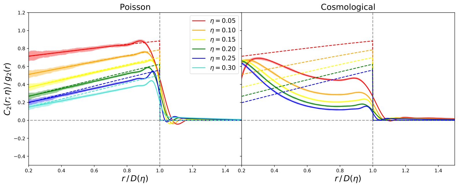
The direct-connectedness function also plays an important role in the analysis of connected systems, in part due to its appearance in the Ornstein-Zernike equation (30). Given $P_{2}(r)$, this can be computed using (31), performing the Fourier transforms numerically via the FFTLog prescription (hamilton2000). Figure 8 shows $C_{2}(r,\eta)$ for both the cosmological and Poisson simulations, alongside the analytic ‘Percus-Yevick’ model, which solves the OZ equation by asserting that $C_{2}(r>D,\eta)=0$ and $P_{2}(r<D,\eta)=1$ (percus-yevick).⁷⁷ 7 This is computed for point objects by using the correspondence with the known (cubic) form for hard spheres via $C_{2}^{\rm PY,Poiss}(r,\eta)=-C_{2}^{\rm PY,hard\,sphere}(r,-\eta)$ (Stell_1984). For the Poisson case, we find good agreement between theory and simulations for small $\eta$ (far from the percolation threshold of $\eta_{c}\approx 0.34$), particularly away from the boundary at $r=D(\eta)$. We observe very little power from the region with $r>D(\eta)$, since most intra-cluster path-ways with $r>D(\eta)$ contain at least one node, and thus do not contribute to $C_{2}(r)$. The cosmological simulations show a very different behavior, with two peaks observed, with one in similar location to the Poisson system and one at smaller $r$. This statistic represents the complexities of the clustering on smaller scales than that typically seen in $P_{2}$ (with $D(\eta)\sim 10h^{-1}\mathrm{Mpc}$), and the differences arise primarily due to small-scale physics, such as the restriction that galaxies cannot be arbitrarily close together. We also note that $C(r,\eta)$ was found to be ill-behaved for $\eta\gtrsim 0.3$ (due to $P_{2}(r,\eta)$ not being square integrable), indicating that the cosmological simulations have percolated by around this value of $\eta$ (cf. §V). In practice, we expect the percolation threshold to depend on the peculiarities of the galaxy sample in question: this will be discussed further below.