A Mean-Field Control Problem of Optimal Portfolio Liquidation with Semimartingale Strategies

The impact of limited liquidity on optimal trade execution has been extensively analyzed in the mathematical finance literature in recent years. The majority of the optimal portfolio liquidation literature allows for one of two possible price impacts. The first approach, pioneered by Bertsimas and Lo [11] and Almgren and Chriss [5], divides the price impact in a purely temporary effect, which depends only on the present trading rate and does not influence future prices, and in a permanent effect, which influences the price depending only on the total volume that has been traded in the past. The temporary impact is typically assumed to be linear in the trading rate, leading to a quadratic term in the cost functional. The original modeling framework has been extended in various directions including general stochastic settings with and without model uncertainty and multi-player and mean-field-type models by many authors including Ankirchner et al. [6], Cartea and Jaimungal [18], Fu et al. [29, 30, 32], Gatheral and Schied [35], Graewe et al. [37], Horst et al. [45], Kruse and Popier [48] and Neuman and Voß [51].

A second approach, initiated by Obizhaeva and Wang [52], assumes that price impact is not permanent, but transient with the impact of past trades on current prices decaying over time. When impact is transient, one often allows for both absolutely continuous and singular trading strategies. When singular controls are admissible, optimal liquidation strategies usually comprise large block trades at the initial and terminal time. The work of Obizhaeva and Wang has been extended by Alfonsi et al. [4], Chen et al. [21], Fruth et al. [27], Gatheral [34], Horst and Naujokat [43], and Predoiu et al. [54], among others.

For single-player models Graewe and Horst [36] and Horst and Xia [44] combined instantaneous and transient impacts into a single model. Although only absolutely continuous trading strategies were admissible in both papers, numerical simulations reported in [36] suggest that if all model parameters are deterministic constants, as the instantaneous impact parameter converges to zero the optimal portfolio process converges to the optimal solution in [52] with two block trades and a constant trading rate.

The recent work of Horst and Kivman [42] provides a rigorous convergence analysis within a Markovian factor model. They proved that in the stochastic setting, the optimal portfolio processes obtained in [36] converge to a process of infinite variation with jumps as the instantaneous market impact parameter converges to zero and showed that the limiting portfolio process is of infinite variation and is optimal in a liquidation model with general semimartingale execution strategies. As such, their work provides a microscopic foundation for the use of semimartingale strategies in portfolio liquidation models.

Liquidation models with inventory processes of infinite variation and semi-martingale strategies were first considered by Lorenz and Schied [49] and Gârleanu and Pedersen [33]. Later, Becherer et al. [10] considered a trading framework with generalized price impact and proved that the cost functional depends continuously on the trading strategy, considered in several topologies. More recently, Ackermann et al. [1] considered a liquidation model with general RCLL semimartingale trading strategies. In a follow-up paper [2] the same authors showed how to reduce liquidation problems with block-trades to standard LQ stochastic control problems. The main difficulty in [1, 2] arises from allowing a very general filtration while we consider a Brownian filtration but allow for self-exciting order flow which results in the said mean-field control problem.

Carmona and Webster [17] provide empirical evidence that inventories of large traders do indeed have a non-trivial quadratic variation component. For instance, for the Blackberry stock, they analyze the inventories of “the three most active Blackberry traders” on a particular day, namely CIBC World Markets Inc., Royal Bank of Canada Capital Markets, and TD Securities Inc. From their data, they “suspect that RBC (resp. TD Securities) were trading to acquire a long (resp. short) position in Blackberry” and found that the corresponding inventory processes were with infinite variation. More generally, they find that systematic tests “on different days and other actively traded stocks give systematic rejections of this null hypothesis [quadratic variation of inventory being zero], with a $p$-value never greater than $10^{-5}$.”

In this paper we consider a single player liquidation model with semi-martingale strategies and expectations feedback where the large investor expects his current trading activity to have an impact on future market dynamics. There are many reasons why (large) orders may have an impact on future price dynamics. For instance, extensive selling may diminish the pool of counterparties and/or generate herding effects where other market participants start selling in anticipation of further price decreases. Extensive selling may also attract predatory traders that employ front-running strategies; see Brunnermeier and Pedersen [12], Carlin et al. [16] and Schied and Schöneborn [56] for an in-depth analysis of predatory trading.

Single and multi-player liquidation models with expectation feedback and absolutely continuous strategies where $dZ_{t}=\xi_{t}dt$ have been considered by, e.g. Cayé and Muhle-Karbe [20] and more recently Chen et al. [22] and Fu et al. [32]. While Cayé and Muhle-Karbe [20] assume an exogenous augmentation of the large trader’s order flow, due to e.g., predatory traders, Chen et al. [22] and Fu et al. [32] assume that the market order dynamics follows a Hawkes process with exponential kernel, and that the large investor’s trading triggers an additional flow of child orders whose rate increases linearly in the investor’s expected traded volume. We retain the assumption of market order arrivals following Hawkes processes but allow for general semi-martingale execution strategies. This results in a novel mean field control problem.

While the restriction to absolutely continuous controls is standard in much of the liquidation literature, the assumption seems restrictive; it is often made for mathematical convenience as the resulting control problem is much simpler to analyze. In fact, while abstract existence and characterization of solutions results can be obtained for models allowing for more general classes of admissible strategies (see [43] and references therein), explicit solutions in stochastic settings are rarely available. Retaining the assumption that the large investor’s trading activity triggers an absolutely continuous flow of child orders that increases linearly in his/her traded volume, we obtain explicit solutions for both the value function and the optimal strategy when allowing for general càdlàg semimartingale trading strategies.

To the best of our knowledge, we are the first to address mean field control problems with càdlàg semimartingale strategies, which include mean field singular control problems as special cases. Mean field singular control problems have been considered by many authors, including [31, 38, 40, 46]. Among them, using a relaxed approach Fu and Horst [31] established an existence of optimal control result for a general class of mean field singular control problems. Guo et al. [38] established a novel Itô’s formula for the flow of measures on semimartingales; however, the examples provided in [38] are mean field control problems with either regular or singular controls. Hafayed [40] established a maximum principle for a general class of mean field type singular control problems. Using a maximum principle approach, Hu et al. [46] studied mean field type singular control games arising in harvesting problems.

Our paper also contributes to the literature on the characterization of non-Markovian singular control problems. One-dimensional models were studied in, e.g. [7, 8, 9, 49]. Multidimensional problems are much more difficult to analyze, even in Markovian settings; see Dianetti and Ferrari [24]. For non-Markovian ones, refer to e.g. [1, 26]. In [1], Ackermann et al. solved a two-dimensional problem with random coefficients arising in optimal liquidation problems. In [26], Elie et al. studied a multidimensional path-dependent singular control problem arising in utility maximization problems. Our control problem is a three-dimensional non-Markovian one with the non-Markovianity arising from a possibly non-Markovian volatility process $\sigma$ and the mean field term $\mathbb{E}[X]$. Moreover, our strategy is of infinite variation.

The main challenge when analyzing control problems with semimartingale strategies (with or without mean-field term) is that there are usually no canonical candidates for the value functions and/or the optimal strategies. Even the linear-quadratic case is difficult to analyze; although it is intuitive that the value function is of linear-quadratic form, the dynamics of the coefficients is a priori not clear. This calls for case-by-case approaches when analyzing such problems. We follow the approach taken in [1, 33] and consider a sequence of discrete time models and then pass to a heuristic continuous time limit. Our approach suggests that the value function depends on the state process only through its distribution and that it is of linear quadratic form driven by three deterministic processes and a BSDE.

It turns out that the driving processes follow a system of Riccati equations that does not satisfy the assumptions that are usually required to guarantee the existence and uniqueness of a solution. Our main mathematical contribution is to show - through a sophisticated transformation - that our system can be rewritten in terms of a more standard system that satisfies the assumption in Kohlmann and Tang [47] under a weak interaction condition that bounds the impact of the child order flow on the market dynamics. Subsequently, we employ a non-standard verification argument that shows that the candidate optimal strategy is indeed optimal. The key idea is to rewrite the cost function as a sum of complete squares plus a correction term that turns out to be the value function.

Our analysis shows that the optimal strategy jumps only at the beginning and the end of the trading period. This is consistent with earlier findings in [33, 42, 43, 52]; in the absence of an external “trigger” there is no reason for the optimal strategy to jump, except at the terminal time to close the position and at the initial time.

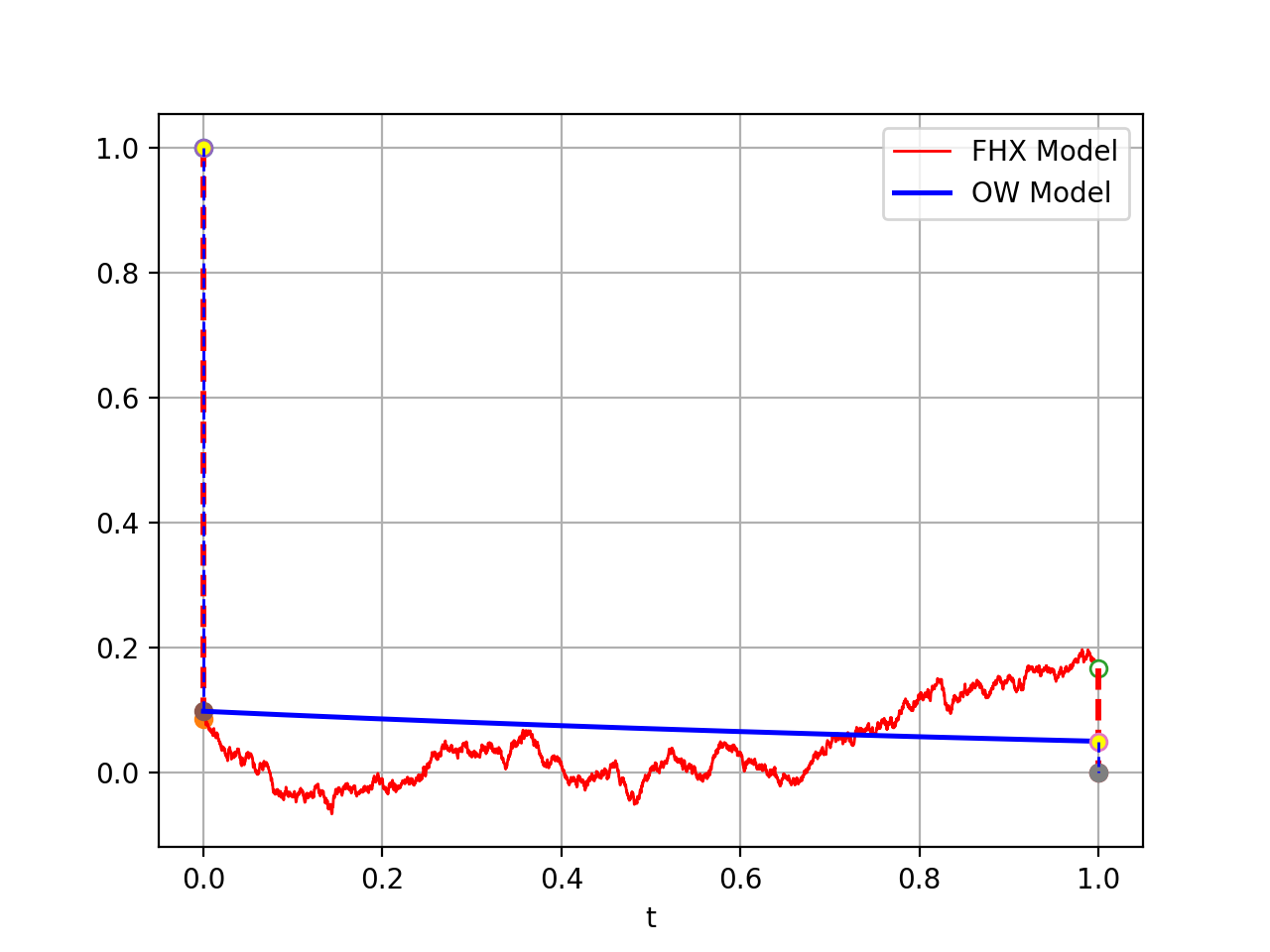
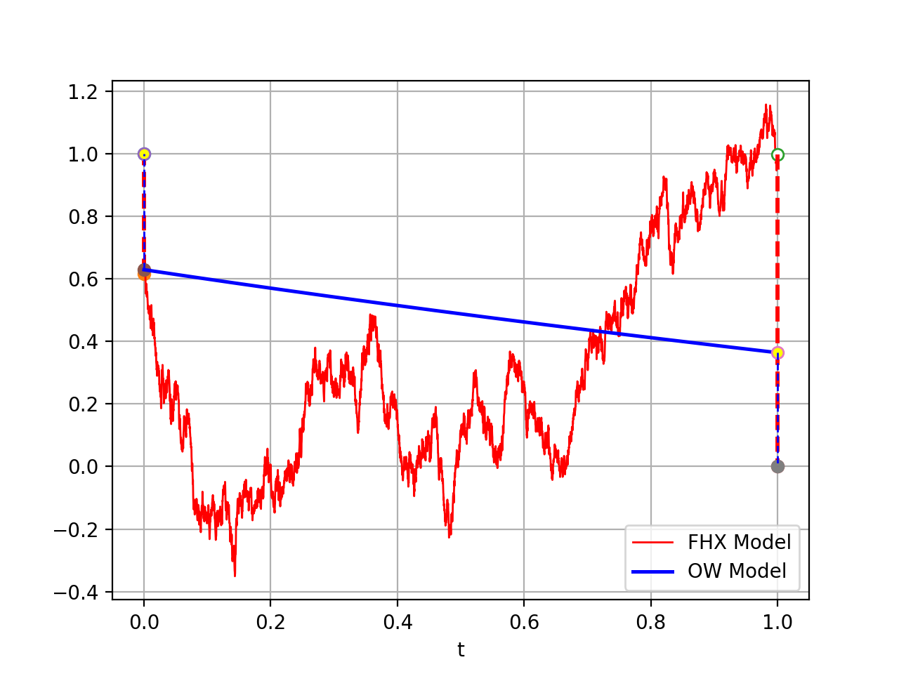
The remainder of this paper is structured as follows. The models, main results and assumptions are stated in Section 2. The wellposedness of the system of the Riccati equations that specify the candidate value function and strategy is established in Section 3. The verification argument is given in Section 4. Numerical simulations illustrating the nature of the optimal solution are given in Section 5. Section 6 concludes. The heuristic derivation of the value function is postponed to an appendix.

Notation. For a deterministic function $\mathcal{Y}$, denote by $\dot{\mathcal{Y}}$ its derivative. For a stochastic process $\mathcal{Y}$ satisfying some SDE, we still use the same notation $\dot{\mathcal{Y}}$ to denote the drift of $\mathcal{Y}$. For a matrix (or vector) $\mathcal{Y}$, $\mathcal{Y}_{ij}$ (or $\mathcal{Y}_{i}$) denotes its $(i,j)$- (or $i$-) component. For a space $\mathcal{D}$, we denote by $L^{\infty}([0,T];\mathcal{D})$ the space of all $\mathcal{D}$-valued bounded functions. $C([0,T];\mathcal{D})$ is the space of $\mathcal{D}$-valued continuous functions. For an integer $n$, we denote by $\mathbb{S}^{n}$ the space of symmetric $n\times n$ matrices. For a measure $\mu$ on ${\mathbb{R}}^{n}$ we denote by $\bar{\mu}$ the vector of expected values, and for a matrix $A\in\mathbb{R}^{n\times n}$ we put

We consider an investor that needs to unwind an initial of $x_{0}$ shares over a finite time horizon $[0,T]$ using general semi-martingale execution strategies $Z$. The large investor’s stochastic control problem at time $t\in[0,T]$ is given by

subject to the state dynamics

for $0\leq s\leq T$, where the set of admissible controls is given by the set

of all square integrable semi-martingales with finite expected covariation.

The process $(X_{t})_{t\in[0,T]}$ describes the investor’s portfolio holdings (“inventory”) with the terminal state constraint $X_{T}=0$ reflecting the liquidation constraint. The process $(Z_{t})_{t\in[0,T]}$ is the trading strategy and $(Y_{t})_{t\in[0,T]}$ specifies the transient impact of the investor’s past trading on future transaction prices. We think of $Y$ as an additional drift “added” to an unaffected martingale price process $M$ that increases linearly in the investors order flow, changes continuously due to noise trader effects, and recovers from past trading at a constant rate $\rho\geq 0$. That is, we assume that the transaction price process is of the form

The martingale part drops out of the equation when computing the expected cost from trading, which are hence given by $\mathbb{E}\left[\int_{0}^{T}Y_{s-}\,dZ_{s}\right]$. This explains the first term in our cost function. The fourth term captures market risk and penalizes slow liquidation. These two terms are standard in the liquidation literature; see [3, 6, 19, 29, 43, 45, 53] and references therein.

When working with semimartingale strategies one additionally needs to penalize the (co)variation of the semimartinagle strategy (with the driving Brownian motion); otherwise the optimization problem is not well posed. This observation goes back at least to Gârleanu and Pedersen [33]; see also [1, 42, 49]. This explains the second and third term in our cost function.

We are now going to introduce an additional feedback effect into the above model that accounts for the possibility of an additional order flow (“child orders”) triggered by the large investor’s trading activities. Specifically, we assume that the transaction price impact process satisfies a dynamics of the form

where the process $(C_{t})_{t\in[0,T]}$ specifies the large investor’s assessment of the impact of child orders triggered by his own trading on the price impact process.

To motivate the dynamics of the endogenous child order term, let us assume as in [22, 32] that market sell and buy orders arrive according to independent exponential Hawkes processes $N^{\pm}$ with respective intensities

Here, $\mu^{\pm}$ are endogenous base intensities that will be specified below, and $\alpha,\beta$ are exogenous deterministic coefficients that capture the impact of past orders on future order flow. The total order flow imbalance can be written as a sum

of the trader’s contribution $Z$ and the endogenous child order process $\cal C$. Working with the child order process is inconvenient. It is much more convenient to consider instead the expected child order process as a measure for the impact of own trading on future transaction price dynamics in (2.4), i.e. to set¹¹ 1 Working with the expected child order process will allow us to work with the child order arrival rate and also accounts for the fact that child orders are not directly observable. We further comment on the choice of the expected child order process below.

We assume that the market is in equilibrium - i.e. that $\mu^{\pm}\equiv\mu$ - if the large investor is inactive. In this case, the order flow imbalance $N^{+}-N^{-}$ is a martingale and hence $C_{t}\equiv 0$. If the large investor employs a continuous semi-martingale strategy of the form

it seems natural to change the base intensities to

where $b^{\pm}_{t}$ denotes the positive/negative part of $b_{t}$. In other words, we assume that the market order arrival intensities increase in the large investor’s trading with the martingale part of his trading strategy having no impact on future order flow.

Since the compensated Hawkes processes $\left(N^{\pm}_{t}-\int_{0}^{t}\zeta^{\pm}_{s}ds\right)_{0\leq t\leq T}$ are martingales starting in zero, the expected child order flow equals

With our choice of base intensities the expected intensities satisfy

As a result, the expected aggregate order flow imbalance $N_{t}:=\mathbb{E}[N^{+}_{t}-N^{-}_{t}]$ equals

and hence the expected number of child orders equals

Differentiating the above equation shows that²² 2 Essentially, it makes no difference to consider $x_{0}$ as random or deterministic. Here, we assume it is a square integrable r.v..

In particular, the child order flow rate resulting from the order submission rate $b$ increases linearly in the expected traded volume $\mathbb{E}[x_{0}]-\mathbb{E}[X_{t}]$ and is mean-reverting if $\frac{\alpha}{\beta}<1$. In this case, each order triggers less than one child order on average and the Hawkes process is stable in the long run; see [41] for details.

Choosing the child order dynamics (2.7) in (2.4) our transient impact process follows the dynamics

In particular, the dynamics of the transient impact process $Y$ can be decomposed into three components³³ 3 Note that a similar decomposition also appears in [50]., namely, the transient impact of the larger trader’s own trading activity

the transient impact of the child orders

and the transient impact of noise traders’ activities

We are now ready to state the large trader’s optimization problem when general semi-martingale strategies are allowed. We retain the assumption that the cost functional at time $t\in[0,T)$ is given by

We also assume that the child order flow is mean-reverting and that it increases linearly in the expected traded volume $\mathbb{E}[x_{0}]-\mathbb{E}[X_{t}]$. In other words, we assume that the impact process satisfies (2.4). The trader’s control problem at time $t\in[0,T]$ is thus given by

subject to the state dynamics

where the set of admissible trading strategies is given by.

References

• [1] J. Ackermann, T. Kruse, and M. Urusov. Càdlàg semimartingale strategies for optimal trade execution in stochastic order book models. Finance and Stochastics, 25(4):757–810, 2021.
• [2] J. Ackermann, T. Kruse, and M. Urusov. Reducing Obizhaeva-Wang type trade execution problems to LQ stochastic control problems. arXiv:2206.03772, 2022.
• [3] A. Alfonsi and P. Blanc. Dynamic optimal execution in a mixed-market-impact Hawkes price model. Finance and Stochastics, 20(1):183–218, 2016.
• [4] A. Alfonsi, A. Fruth, and A. Schied. Optimal execution strategies in limit order books with general shape functions. Quantitative Finance, 10(2):143–157, 2010.
• [5] R. Almgren and N. Chriss. Optimal execution of portfolio transactions. Journal of Risk, 3:5–40, 2001.
• [6] S. Ankirchner, M. Jeanblanc, and T. Kruse. BSDEs with singular terminal condition and a control problem with constraints. SIAM Journal on Control and Optimization, 52(2):893–913, 2014.
• [7] P. Bank. Optimal control under dynamic fuel constraint. SIAM Journal on Control and Optimization, 44(4):1529–1541, 2005.
• [8] P. Bank and N. El Karoui. A stochastic representation theorem with applications to optimization and obstacle problems. Annals of Probability, 32(1B):1030–1067, 2004.
• [9] P. Bank and F. Riedel. Optimal consumption choice with intertemporal substitution. Annals of Applied Probability, 11(3):750–788, 2001.
• [10] D. Becherer, T. Bilarev, and P. Frentrup. Stability for gains from large investors’ strategies in M1/J1 topologies. Bernoulli, 25(2):1105–1140, 2019.
• [11] D. Bertsimas and A. Lo. Optimal control of execution costs. Journal of Financial Markets, 1(1):1–50, 1998.
• [12] M.K. Brunnermeier and L.H. Pedersen. Predatory trading. Journal of Finance, 60(4):1825–1863, 2005.
• [13] L. Campi, T. De Angelis, M. Ghio, and G. Livieri. Mean-field games of finite-fuel capacity expansion with singular controls. to appear in Annals of Applied Probability, 2020.
• [14] H. Cao, J. Dianetti, and G. Ferrari. Stationary discounted and ergodic mean field games of singular control. to appear in Mathematics of Operations Research, 2021.
• [15] H. Cao and X. Guo. MFGs for partially reversible investment. to appear in Stochastic Processes and their Applications, 2020.
• [16] B. Carlin, M. Lobo, and S. Viswanathan. Episodic liquidity crises: Cooperative and predatory trading. Journal of Finance, 62(5):2235–2274, 2007.
• [17] R. Carmona and K. Webster. The self-financing equation in limit order book markets. Finance and Stochastics, 23(3):729–759, 2019.
• [18] Á. Cartea and S. Jaimungal. Incorporating order-flow into optimal execution. Mathematics and Financial Economics, 10(3):339–364, 2016.
• [19] Á. Cartea, S. Jaimungal, and J. Ricci. Algorithmic trading, stochastic control, and mutually exciting processes. SIAM Review, 60(3):673–703, 2018.
• [20] T. Cayé and J. Muhle-Karbe. Liquidation with self-exciting price impact. Mathematics and Financial Economics, 10(1):15–28, 2016.
• [21] N. Chen, S. Kou, and C. Wang. A partitioning algorithm for markov decision processes with applications to market microstructure. Management Science, 64(2):784–803, 2018.
• [22] Y. Chen, U. Horst, and H. Tran. Optimal trade execution under endogenous order flow. https://ssrn.com/abstract=3933364, 2021.
• [23] A. Cosso and H. Pham. Zero-sum stochastic differential games of generalized McKean–Vlasov type. Journal de Mathématiques Pures et Appliquées, 129:180–212, 2019.
• [24] J. Dianetti and G. Ferrari. Multidimensional singular control and related Skorokhod problem: sufficient conditions for the characterization of optimal controls. arXiv:2103.08487, 2021.
• [25] J. Dianetti, G. Ferrari, M. Fischer, and M. Nendel. A unifying framework for submodular mean field games. to appear in Mathematics of Operations Research, 2022.
• [26] R. Elie, L. Moreau, and D. Possamaï. On a class of path-dependent singular stochastic control problems. SIAM Journal on Control and Optimization, 56(5):3260–3295, 2018.
• [27] A. Fruth, T. Schöneborn, and M. Urusov. Optimal trade execution and price manipulation in order books with time-varying liquidity. Mathematical Finance, 24(4):651–695, 2014.
• [28] G. Fu. Extended mean field games with singular controls. SIAM Journal on Control and Optimization, 61(1):285–314, 2023.
• [29] G. Fu, P. Graewe, U. Horst, and A. Popier. A mean field game of optimal portfolio liquidation. Mathematics of Operations Research, 46(4):1235–1657, 2021.
• [30] G. Fu, P. Hager, and U. Horst. Mean-field liquidation games with market drop-out. arXiv:2303.05783, 2023.
• [31] G. Fu and U. Horst. Mean field games with singular controls. SIAM Journal on Control and Optimization, 55(6):3833–3868, 2017.
• [32] G. Fu, U. Horst, and X. Xia. Portfolio liquidation games with self-exciting order flow. Mathematical Finance, 32(4):1020–1065, 2022.
• [33] N. Gârleanu and L.H. Pedersen. Dynamic portfolio choice with frictions. Journal of Economic Theory, 165:487–516, 2016.
• [34] J. Gatheral. No-dynamic-arbitrage and market impact. Quantitative Finance, 10:749–759, 2011.
• [35] J. Gatheral and A. Schied. Optimal trade execution under geometric Brownian motion in the Almgren and Chriss framework. International Journal of Theoretical and Applied Finance, 14(3):353–368, 2011.
• [36] P. Graewe and U. Horst. Optimal trade exection with instantaneous price impact and stochastic resilience. SIAM Journal on Control and Optimization, 55(6):3707–3725, 2017.
• [37] P. Graewe, U. Horst, and J. Qiu. A non-Markovian liquidation problem and backward SPDEs with singular terminal conditions. SIAM Journal on Control and Optimization, 53(2):690–711, 2015.
• [38] X. Guo, H. Pham, and X. Wei. Itô’s formula for flow of measures on semimartingales. to appear in Stochastic Processes and Their Applications, 2020.
• [39] X. Guo and R. Xu. Stochastic games for fuel followers problem: N vs MFG. SIAM Journal on Control and Optimization, 57(1):659–692, 2020.
• [40] M. Hafayed. A mean-field necessary and sufficient conditions for optimal singular stochastic control. Communications in Mathematics and Statistics, 1:417–435, 2013.
• [41] A. Hawkes and D. Oakes. A cluster process representation of a self-exciting process. Journal of Applied Probability, 11(3):493–503, 1974.
• [42] U. Horst and E. Kivman. Optimal trade execution under small market impact and portfolio liquidation with semimartingale strategies. to appear in Finance and Stochastics, 2022.
• [43] U. Horst and F. Naujokat. When to cross the spread? Trading in two-sided limit order books. SIAM Journal on Financial Mathematics, 5(1):278–315, 2014.
• [44] U. Horst and X. Xia. Multidimensional optimal trade execution under stochastic resilience. Finance and Stochastics, 4(23):889–923, 2019.
• [45] U. Horst, X. Xia, and C. Zhou. Portfolio liquidation under factor uncertainty. Annals of Applied Probability, 32(1):80–123, 2022.
• [46] Y. Hu, B. Øksendal, and A. Sulem. Singular mean-field control games. Stochastic Analysis and Applications, 35(5):823–851, 2017.
• [47] M. Kohlmann and S. Tang. Multidimensional backward stochastic Riccati equations and applications. SIAM Journal on Control and Optimization, 41(6):1696–1721, 2003.
• [48] T. Kruse and A. Popier. Minimal supersolutions for BSDEs with singular terminal condition and application to optimal position targeting. Stochastic Processes and their Applications, 126(9):2554–2592, 2016.
• [49] C. Lorenz and A. Schied. Drift dependence of optimal trade execution strategies under transient price impact. Finance and Stochastics, 17(4):743–770, 2013.
• [50] J. Muhle-Karbe, Z. Wang, and K. Webster. Stochastic liquidity as a proxy for nonlinear price impact. 10.2139/ssrn.4286108, 2022.
• [51] E. Neuman and M. Voß. Optimal signal-adaptive trading with temporary and transient price impact. SIAM Journal on Financial Mathematics, 13(2):551–575, 2022.
• [52] A. Obizhaeva and J. Wang. Optimal trading strategy and supply/demand dynamics. Journal of Financial Markets, 16(1):1–32, 2013.
• [53] A. Popier and C. Zhou. Second order BSDE under monotonicity condition and liquidation problem under uncertainty. Annals of Applied Probability, 29(3):1685–1739, 2019.
• [54] S. Predoiu, G. Shaikhet, and S. Shreve. Optimal execution in a general one-sided limit-order book. SIAM Journal on Financial Mathematics, 2(1):183–212, 2011.
• [55] P. E. Protter. Stochastic Integration and Differential Equations. Springer, 2005.
• [56] A. Schied and T. Schöneborn. Liquidation in the face of adversity: Stealth vs. sunshine trading. ssrn.1007014, 2009.