Higgstory repeats itself
Alessandro Strumiaa and Nikolaos Tetradisb,c
a Dipartimento di Fisica, Università di Pisa, Italia
b Department of Physics, National and Kapodistrian University of Athens, Greece
c CERN, Theoretical Physics Department, Geneva, Switzerland
Abstract
We consider a scalar potential with two minima, one of which is arbitrarily deep, such as could be the case for the Higgs potential in the Standard Model. A recent calculation within the thin-wall approximation [1] concludes that regions in which the scalar field takes values beyond the top of the potential barrier are forced by gravity to collapse, while they remain hidden behind a black hole horizon. We show that the thin-wall approximation is not applicable to this problem. We clarify the issue through numerical and analytical solutions to the field equations of the gravity-scalar system. We find that regions around the deeper minimum expand, and would thereby engulf the Universe in post-inflationary cosmology. We also show that black holes with Higgs hair are unstable. Even though the physics of the true vacuum is different, our final conclusion replicates the earlier ‘Higgstory’ paper [2].
1 Introduction
A decade ago the Higgs boson mass was measured [3, 4], and its value implied the possible instability of the Standard Model Higgs potential at large field values [5, 6, 7]. This instability would have important cosmological implications [2, 5, 8, 9, 10, 11, 12, 13, 14, 15, 16, 17]. Establishing if the SM Higgs potential is really unstable needs a more accurate determination of the top quark mass, a task that seems feasible only at a future lepton collider at the threshold [18, 19], possibly in the LEP tunnel [20].
Motivated by this possible instability, we reconsider a more general cosmological issue: if a scalar sits at the local minimum of a potential that also has a deeper minimum at (so that ) beyond a potential barrier at , what is the fate of space-time regions where the field acquires values ? As the field tends to roll down towards the deeper minimum, one expects that such regions would grow in space, assuming that they are large enough for the potential energy to dominate over gradient energy.
The situation is less clear when gravity is taken into account, as regions with negative energy density tend to undergo an AdS-like gravitational collapse towards an uncertain final state. This problem was studied in [2] (‘Higgstory’ paper), where such regions were approximated as thin-wall spherical bubbles with inside and outside. It was found that an observer inside the bubble experiences an AdS crunch, while an outside observer sees the bubble expand. When this picture is applied to the SM case, it implies that expanding bubbles would engulf the whole universe once inflation ends. This is not observed, implying bounds on cosmology, in particular on the inflationary Hubble scale [2, 12, 13, 15, 16, 17].
A recent paper [1] reaches a different conclusion by extending the thin-wall approximation used in [2] to analyze also the earlier phase during which falls down the potential towards . This phase was not studied in [2]. However, for a very deep true vacuum, or an unbounded potential, it may play a crucial role in the evolution of the system. The authors of [1] correctly point out that the energy density inside the bubble decreases towards zero (as rolls down the potential, while the kinetic energy is red-shifted away by the Hubble friction), until the local scale factor stops expanding and starts to contract. Subsequently, gets blue-shifted and becomes dominant during the rapid fall of towards the true minimum, with a singularity developing if the minimum is very deep. However, [1] also claims that, as a result, the thin wall of the bubble starts moving inward until it disappears, hidden beyond a static black hole horizon. The exterior space-time remains largely unaffected, apart from the appearance of an isolated black hole.
This is puzzling, as physical systems with stochastic fluctuations are commonly expected to evolve towards vacua with lower energy and eventually find their way to the true vacuum. If this scenario were true, it would have a big impact on more general similar situations, such as spontaneous vacuum decay to AdS vacua, multiverse inflationary dynamics, ultra-high-energy collisions of cosmic rays [21, 22, 23, 24, 25], or even at colliders and possibly more general Higgs engineering. We thereby re-examine this issue. Even though we confirm the analysis of [1] for the initial stage of the evolution, our final results replicate the original Higgstory [2] conclusion that the bubbles can expand.
The crucial point is that the simplifying thin-wall assumption — an AdS bubble with constant at the minimum inside — was generalized in [1] to an assumption for constant field over the whole interior. However, assuming a constant field value away from the potential minimum is an unphysical ‘rigidity’ assumption that artificially links the inner crunch to the wall boundary, forcing the contraction and disappearance of the whole bubble. In section 2 we show that the thin-wall approximation is not applicable to the general situation with . What happens instead is that even an initially thin wall gets stretched on both sides (in a sense falling down towards either minimum), thus becoming thick. The configuration looks like a ‘sinkhole’.
In order to establish the physical mechanism at work, we derive in section 3 the full equations of the gravity-scalar system, and solve them in multiple ways: we find one analytic solution in one special case, and numerical solutions in generic cases, using two different forms of the dynamical metric (FRW-like or static-like). All solutions lead to the same general conclusion: the process is similar to a gravitational collapse, where an inner region contracts without affecting substantially the outer region, which keeps expanding because the two get causally disconnected and/or because information about the collapse does not propagate fast enough. A black hole forms, but it sits in the true vacuum and thereby is not static, as it accretes energy. In section 4 we explore related configurations that can be described as static black holes with Higgs hair, finding that they are unstable.
Conclusions are given in section 5.
2 The form of the bubbles
We consider a scalar field coupled to gravity. Without loss of generality, a non-minimal scalar coupling to gravity can be removed by a field redefinition, and the system can be studied in the Einstein frame, where both scalar and gravity have canonical kinetic terms. The action then is
| (1) |
where we use the convention for the signature of the metric. We assume that the scalar potential has a false minimum with and a true minimum , possibly very deep. They are separated by a potential barrier . For example, we can consider potentials with of the form
| (2) |
with and . The inflationary energy can be provided by some other scalar, whose nature is not relevant here. We want to establish if a region where expands.
2.1 Description through the matching of geometries
To start, we review aspects of the thin-wall bubble approximation, in order to later state our full numerical results in this simplified language, and to explain why it is not adequate for the problem at hand. An approximate description of the evolving bubble can be obtained by assuming the metric
| (3) |
where . A thin wall located at separates Schwarzschild-de Sitter (SdS) outside with , from Schwarzschild-anti de Sitter (SAdS) inside with , where and are the energy densities. Similar solutions exist if and have the same sign. The solution also contains a central black hole with mass . The metric transverse to is continuous on the wall, while the function has a discontinuity proportional to the wall surface tension , as dictated by the Israel matching condition [26, 27]
| (4) |
Solving for results in an intuitive expression:
| (5) |
where also includes the gravitational energy. Solving eq. (4) for gives
| (6) |
a form useful for studying the motion of the wall, as it is formally similar to the conservation of ‘energy’ for a point in a ‘potential’ that encodes the general-relativistic effects.
The solutions of eq. (6) for were discussed in detail in [2], and the generalization for was given in the appendices of [28]. A general feature is the existence of solutions that describe expanding bubbles. The expansion is energetically favoured for large bubbles, when the interval volume with negative energy density dominates the total energy budget. For example, setting (no black hole inside) and ignoring the last term of eq. (6) (i.e. in the limit ), the sign of indicates that a thin-wall bubble initially at rest expands if , as is also expected from the initial expression for constant .
However, there are two approximations that must be relaxed when developing a formalism that could approximate an evolving field in the interior. They concern the parameters and , which must be allowed to evolve if they are to approximate a time-dependent field configuration. In the rest of this section we discuss the possible implications, before studying the full problem in the following section.
2.2 Interior with a continuous mass distribution
The first step towards a more general description is the replacement of the mass parameter of the SAdS metric with a continuous mass distribution. An analytic description is very difficult for a general equation of state. However, a simple analytic solution exists if is attributed to a pressure-less component. We consider this case as a toy model that illustrates how a result qualitatively different from [1] can arise if we eliminate the rigidity assumption that links the evolution of the bubble surface to that of the interior.
We employ the thin-wall approximation and describe the space inside the bubble through the Tolman-Bondi (TB) metric [29, 30] in the presence of a negative cosmological constant:
| (7) |
The function gives the location of the shell with comoving coordinate as a function of time. It satisfies
| (8) | |||||
| (9) |
The function gives the (conserved) integrated mass of the fluid, up to the shell with coordinate . The function can be viewed as a generalized spatial-curvature term; it will play no role. The coordinate patch covers the part of the space for which the right-hand side of eq. (8) is positive.
The FRW metric, for a space containing a homogeneous pressure-less fluid, is obtained for , , , with . The homogeneous case provides intuition about the nature of the evolution in the interior of the bubble. The resulting Friedmann equation reads
| (10) |
It is apparent that an initially expanding spacetime will stop expanding when reaches a value such that the right-hand side of the above equation vanishes. It will subsequently collapse to a singularity within a finite time . Near the singularity we have and the energy density of the pressure-less fluid gives the dominant contribution, with a time dependence . This is analogous (even though the exponents of the singular terms differ) to the behaviour deduced in [1], where the assumption of homogeneity was also made.
 |
If the matter is concentrated within a radius , so that and for , the geometry outside this region is the standard SAdS geometry. This can be made explicit by matching the interior metric in eq. (3) with the metric in eq. (7) at some through the Israel matching conditions. A smooth matching at requires . In this way the configuration illustrated in fig. 1b appears consisting of: a) a central inhomogeneous region up to , b) a shell of SAdS space up to the bubble surface, c) the bubble surface with constant tension, d) the SdS exterior of the bubble. The evolution of the surface is described by the formalism of the previous subsection. It is clear then that, in this case, the evolution of the bubble surface is blind to the actual mass distribution and is affected only by the total mass. The analysis is identical to [28] and shows that the gravitational collapse, by itself, does not prevent the bubbles from expanding.
The situation is more complicated if the matter distribution extends all the way to the bubble surface. However, a particular case is illuminating. We assume that the nonrelativistic fluid covers the whole interior of an expanding bubble at the time at which . This is the time of the maximal expansion of the interior. At later times the interior starts contracting, so that the shell with comoving coordinate moves inside the bubble. The assumption of a constant bubble tension implies that there is no source of matter on the bubble surface. It is, therefore, expected that a gap will appear between the collapsing matter and the bubble radius. Within this part of space, the metric is of the SAdS form, with . The crucial point is that the evolution of the bubble surface remains unaffected by all that is happening in its interior, so that it can keep expanding. Matter can collapse forming a black hole, while the wall expands outside the horizon.
Allowing for radial inhomogeneities or different initial conditions prohibits a precise description. However, several features of the evolution can be deduced intuitively. The effect of the interior on the bubble evolution is parametrised by the mass function at the location of the surface. In this sense, the relative expansion or contraction of various regions in the interior plays a secondary role. In general, the value of is time-dependent. If it increases with time, matter may either accumulate on the bubble surface, or move into the exterior. The first possibility would violate our assumption of a constant wall tension. The second possibility would result in matter leaking into the region dominated by a positive cosmological constant, where it would be diluted by expansion. This would continue until the interior starts collapsing. These observations indicate that the approximate description of the interior by a SAdS metric with a mass parameter corresponding to the total mass within the bubble gives a reasonable description of the dynamics. The general conclusion is that the bubble evolution is not tied to the collapse of the interior.
Even though this toy model provides an intuitive understanding of the competing features of the evolution, it is not adequate for the description of a fully dynamical field. We turn to this problem next.
2.3 Scalar at its minima and applicability of the thin wall approximation
The ‘Higgstory’ study [2] assumed as initial condition a thin wall bubble with the scalar near to its minima both inside and outside: and . The resulting geometry is exemplified in fig. 2a in the language of eq. (3) and the above formalism implies that such thin-wall bubble can expand.
In this case the thin-wall approximation is adequate because in the subsequent evolution remains close to its minima, and even an initially thick wall becomes thin thanks to its expansion. Indeed the wall tension can be approximated assuming that in a small range the scalar field varies by :
| (11) |
minimised for a bubble thickness comparable to the minimal radius such that the bubble expands. In this case remains fixed during the evolution, so and the shape of the thin wall remain fixed (as assumed in eq. (4)) and only the location of the wall can evolve. For a quartic potential .
2.4 Scalar not at its minima and inapplicability of the thin wall approximation
The recent study [1] considers a different initial condition at an earlier time: the Higgs expectation value inside the bubble, , has not yet reached the minimum of its potential. Rather, the field inside the bubble is assumed to have a value just past the potential barrier, , with the potential inside taking a value much above , . The resulting cosmology is inflationary on either side of the bubble surface, but with a lower expansion rate inside, as illustrated in fig. 2b.
Since falls down the potential towards , the gap in field values grows with time. Therefore, the wall tension , estimated in eq. (11), cannot remain constant in time, unlike what was assumed in [1] (leading to the claim that the bubble disappears). It is not even possible to improve the thin-wall approximation by allowing for a time-dependent wall tension and adding a time-dependent wall pressure. Indeed, if the wall is not surrounded by regions where is at its minimum, the wall has more degrees of freedom than the one corresponding to radial displacement. Even assuming an initially thin wall, the field can now fall down the potential on both sides, getting stretched at roughly the speed of light by an amount . As a simple example of this, fig. 1 displays the numerical solution to the classical Higgs equation of motion (in the usual notation , , ), assuming a spherical Higgs field configuration in the SM potential that is approximated through an effective running coupling as
| (12) |
The electroweak vacuum is located at , while the true minimum is so deep that its existence plays no significant role. Fig. 1 shows that an initial thin-wall field profile is not maintained in the following time evolution. The potential energy of the system resembles a sinkhole rather than a wall. As the fall of inside proceeds, the potential barrier in becomes negligible and the scalar field profile approaches a different general form: deeper where it had more time to fall. This kind of time evolution is expected to be general, since it only depends on local physics around the initially thin wall. The wall evolution violates the assumption, used to justify the thin-wall approximation, that the domain wall settles into an equilibrium configuration (see e.g. section III of [27]).
After a time of order 11 1 Indeed, the solution to is assuming a constant and an -independent initial field value at . the Higgs fall reaches the deep minimum and bounces back, or hits a singularity if the potential is approximated as unbounded from below.
We emphasize that the subsequent evolution is computable even after the formation of the singularity, in the region outside its light-cone and thereby not causally affected by the singularity. The generic outcome is that the bubble keeps expanding at the speed of light. The simplest computable example of this phenomenon is a potential with in flat space, as the classical equation admits the Fubini solution
| (13) |
This solution describes a thick wall that keeps expanding at the speed of light after that the singularity appears at a time . One way of obtaining numerical solutions consists in ‘regularising’ the divergence by adding to the potential a deep true vacuum, such that the region affected by the singularity is replaced by the scalar field oscillating around the minimum, while the causally disconnected region at large value of is not affected. Overall, the system is analogous to a sinkhole in the ground that keeps expanding while the parts near the surface keep sliding down, irrespectively of the fact that its central region might be infinitely deep.
The above discussion and the numerical simulation in fig. 1 have neglected gravity. According to [1] gravity adds one key new effect: a thin-wall bubble disappears in a gravitational collapse, getting fully hidden behind a horizon. Since we have argued that the system cannot be approximated by a thin wall, we expect that the scalar field dynamics, together with gravitational dynamics, will remove the inner part of the system, but the outer part that unavoidably develops (even around an initially thin wall) will survive and keep expanding.
Even if only one bubble finds a way to expand and engulf the Universe, the usual bounds (see [2] and subsequent papers) apply. This makes it possible to settle the issue through an example. We thereby proceed to solve the equations of the gravity-Higgs system in section 3 in order to produce numerical examples, as well as a particular analytic solution.
3 Gravitational Higgs sinkhole
In section 3.1 we present a special analytic solution that describes a scalar rolling down its potential, taking gravity into account. We next obtain numerical solutions in generic situations. To cross-check our results we use two different ansatze for a metric with spherical symmetry: reparametrization invariance is used in section 3.2 to make the time dependence explicit, resulting in a FRW-like metric; while in section 3.3 the radial dependence is made explicit, resulting in a Schwarzschild-like metric.
Before presenting the solutions, we recall a tool that will help the interpretion of singularities appearing in time-dependent spherically symmetric geometries. An apparent horizon is defined as the boundary of the region of trapped surfaces. This boundary is a surface on which the expansion of outgoing null geodesics vanishes. In order to determine the presence of such a horizon, we examine the expansion of radial null geodesics. The two sets of geodesics, generically denoted by , can be determined from the metric. In flat space , so that the solutions and clearly correspond to outgoing and ingoing null geodesics, respectively. However, in non-trivial geometries, and especially in the vicinity of horizons, a more careful analysis is necessary in order to determine their nature. (Despite this, we always refer to the geodesics as out/ingoing, for simplicity). For a spherically symmetric geometry, the true nature of the geodesics becomes clear if we consider that they define surfaces of areal radii . A truly outgoing geodesic results in the growth of the area of such a surface, while an ingoing geodesic results in the reduction of the area. On an apparent horizon, the rate of change of the area vanishes. The product
| (14) |
is a convenient quantity in order to search for horizon as it is independent of the normalization of the vectors that define the null hyper-surfaces. In flat space so . An apparent horizon would appear at the point where vanishes before changing sign.
  |
3.1 Special analytic solution
We start by presenting a special analytic solution for an expanding scalar bubble in general relativity. It is obtained starting from the analytic Fubini solution of eq. (13), valid in the absence of gravity for a purely quartic scalar potential. Since the potential is scale-invariant, eq. (13) remains a solution even in the presence of gravity, provided that the scalar has a conformal coupling to gravity. Starting from this solution and rewriting the system in the Einstein frame in terms of a canonically normalized scalar , one obtains the potential
| (15) |
The Einstein and scalar-field equations have the solution
| (16) |
with a conformally-flat metric, arbitrary , and .
This solution is visualised in fig. 3. The singularity with , and infinite curvature first develops at at a time . At later times the location of the singularity moves to finite values of . However, vanishes at the same , so that physical distances, such as the areal distance , also vanish.
As discussed above, an apparent horizon is present if , defined in eq. (14), vanishes. In this example, outgoing/ingoing geodesics for the metric of eq. (16) satisfy , while the areal radius is . This gives
| (17) |
As illustrated in fig. 3, the singularity is always surrounded by the apparent horizon. Overall, the analytic solution is qualitatively similar to the generic cases computed via numerical tools and presented in the following subsections. It clearly shows that the bubble keeps expanding at the speed of light, even after the formation of the singularity, with the total energy density becoming positive.22 2 The analytic continuation of our solution into the region behind the singularity can be interpreted as the creation of a Universe induced by scalar inflation. This provides a simple counter-example to the possibility of a general gravitational mechanism that prevents bubble expansion.
3.2 Metric in time-friendly FRW form
A spherical non-homogeneous system can be described by the time-friendly FRW-like metric [30]
| (18) |
so that is a simple time parameter and is the areal distance. The resulting field equations contain second time derivatives for all fields :
|
We numerically solve the equations for a potential of the form of eq. (2). The barrier is at in the relevant bottom-less limit . We consider the initial condition , , at . The initial field profile is assumed to be
| (20) |
The parameters and of the initial configuration must be chosen such evolves towards its true minimum.
- •
We choose beyond the potential barrier but still in the region where , such that one has inflationary de Sitter space with Hubble constant at , and de Sitter with lower Hubble constant at .
- •
Furthermore, as discussed around eq. (11), in the thin-wall limit a bubble expands for , where and are the field and potential variations along the bubble. Beyond the thin-wall limit no such simple criterion for expansion is known, but the thin-wall criterion remains qualitatively correct.
Motivated by inflationary dynamics, we consider a Hubble scale comparable to the size of the bubble. Then for . More precisely, we display the result for the following numerical example33 3 Avoiding large or small numbers helps the computation and the visualization of the numerical solution. Similar results are obtained in the SM-like case, where the key collapse dynamics happens within a small fraction of the time range.
| (21) |
Another important scale of the problem is the time needed for the deep fall of . Taking gravity into account, it is estimated as
| (22) |
by considering a homogeneous Higgs field in a fixed inflationary background: neglecting in its equation , one finds the solution [1].
  |
The quantity of eq. (14), used to deduce the formation of an apparent horizon, becomes
| (23) |
as the out/ingoing null geodesics obey , while the areal distance is , so that eq. (23) follows from . In the homogeneous limit this reduces to , reproducing the usual dS horizon at .
Thick-wall numerical solution
If the true minimum of the potential is not deep, the system evolves in a way qualitatively similar to the flat case: the field reaches , bounces and starts oscillating around the true minimum, while the bubble expands at nearly the speed of light, following the de Sitter geometry of the outer space-time.
In the opposite limit, with a true minimum so deep that its presence is irrelevant, numerical simulations such as the one shown in fig. 4 display the following characteristics. The scale factors initially increase until the total energy density becomes negative around the interior of the bubble (due to the fall of the scalar and to Hubble friction). Within this region and at this point in time the scale factors start decreasing, triggering a run-away accelerated fall of , with energy dominated by the kinetic energy (see fig. 4b). As a result, a singularity in and in the curvature develops, at the point and at a time as in eq. (22). An apparent horizon forms at an earlier time at finite , denoted as ‘H’ in fig. 4a.
In contrast to the thin-wall expectation in [1], a growing region where the scalar is mildly above its potential barrier remains in the region outside the collapse, where the scale factors keep growing.
Regions inside the apparent horizon do not affect the exterior, so that we can keep computing after the singularity develops by dropping regions in its immediate vicinity, confirming that the bubble keeps growing, similarly to the analytic solution of section 3.1. We also point out that the scale factors vanish at the location of the singularity, indicating that the areal distance for this point also vanishes.
The numerical solution shows that the thin-wall claim of [1] cannot be fully general. As one bubble that expands is enough to imply bounds, having demonstrated its existence settles the wider issue. However, in order to obtain a broader perspective we next proceed to examine wall profiles that are initially thin.
  |
Thin-wall numerical solution
In order to highlight the difference with respect to the thin-wall claim of [1], we next evolve a special initial configuration with an initially thin wall, namely the profile in the lower row of eq. (20), such that is piece-wise nearly constant: inside at , and outside at .
We again consider a deep fall of the scalar field (otherwise the scalar soon reaches its true vacuum and bounces back, leading to the usual expanding bubble of true vacuum). The numerical solution in fig. 5 shows that, as expected, the thin wall approximation breaks down. At the beginning the scale factors grow while remaining piece-wise constant, being smaller inside that outside the bubble. Their equality is only violated around the bubble surface An apparent horizon forms around the formerly-thin wall at as soon as the collapse starts in the interior. Indeed grows inside, as gets large and and gets small. As the outside keeps inflating, near the wall there is a point where : here remains small and horizons appear.44 4 Fig. 5 shows a numerical solution with so de Sitter horizons also play a role. The same main features apply for and even with outer Minkowski space, .
In the generic thick-wall configuration of fig. 4 the FRW scale-factors hit the singularity at . In the special initially-thin configuration of fig. 5 the scale factors approach zero at the same time in almost all of the interior. This makes no difference to an outside observer, as this happens when the wall is no longer thin: a growing region with mildly above the instability critical value and size has developed outside. We can measure its size in terms of the physical areal distance : since outside we find that the bubble remains big despite the collapse inside.
In a qualitative sense, the crucial difference with respect to the thin-wall claim of [1], according to which the final state only contains a black hole, is that the black hole lives in the true vacuum rather than in the false vacuum. It is time-dependent as it accretes the energy difference stored in the dynamical scalar field. An outside observer sees an expanding bubble.
3.3 Metric in space-friendly static form
As a check, we next solve again the same physical problem replacing the time-friendly FRW coordinate system with a space-friendly static coordinate choice. The metric is again written in terms of two functions, now called and :
| (24) |
In these coordinates is the areal distance. The classical equations are
|
In these static-like coordinates the equations for the metric factors and contain no time derivatives (unlike what happened with FRW-like coordinates). So the whole system is equivalent to one integro-differential equation for . Since is a time-dilation factor, it becomes irrelevant in the static limit: the equation for separates from the others, as one can see by substituting and in the equation for obtaining
| (26) |
with vanishing left-hand side. Light moves radially as , so time moves faster where is larger. The criterion of eq. (14) for an apparent horizon becomes in static coordinates: a horizon appears where/when time freezes.
By writing , the equation for simplifies into an intuitive equation for the mass enclosed in radius :
| (27) |
If a black hole is present, and one needs to solve the equations only outside its horizon. Convenient boundary conditions for are or : the two coordinate choices describe the same physics, being related by some redefinition of the time coordinate. We follow the standard , so that numerical solutions slow down before hitting the singularity.
For a constant field , the solution i.e. reproduces the well known static dS (for ) and AdS (for ) solutions,
| (28) |
with Hubble rate if . For one has at : this is the usual dS horizon. In the static limit, the static deSitter coordinates (denoted as in the equation below) cover partially the flat FRW coordinates (denoted as ) that, in turn, cover partially the full de Sitter space. Their explicit connection is
| (29) |
The connection between FRW-like and static-like coordinates is more complicated.
  |
Numerical simulations in static-like coordinates
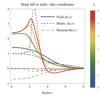
In view of their hybrid nature, we solve numerically eq.s (3.3) in two independent ways: with routines built in Mathematica, or using the implicit Euler method at 2nd order in the discretisation step.
In static coordinates, even an initial configuration that is -independent acquires a dependence on , as the field evolves in time. This can be seen by simply considering a fixed background: the scalar equation becomes , with no Hubble friction in time. Time evolution of a scalar in a fixed dS background happens faster at smaller ; while time evolution in a fixed AdS background happens faster at larger . An initially thin wall does not remain thin because of this effect, in addition to the expansion of the wall. In flat space (), deep fall in a quartic scalar potential happens in a time . This fall time is parametrically the same as the minimal radius needed for an expanding bubble, so that its profile gets significantly distorted.
We assume an initial condition like in eq. (21), except that now with respect to the static-coordinates time and . During the subsequent fall, the kinetic energy density grows, while the potential energy decreases, and the total energy density tends to vary less, in view of the absence of Hubble friction. There is no contradiction with the FRW picture of the previous section, as the energy density (the time-time component of the energy-momentum tensor ) is coordinate-dependent.
The metric factor was initially (under the assumption ). If the potential is shallow the numerical evolution reaches the true minimum ; next the scalar bounces, leading to an expanding bubble while becomes mildly negative in the interior, meaning that ‘time’ of the present coordinates runs slower in the interior.
Fig. 6 shows a solution for a deep scalar fall in an ideally bottom-less potential: becomes largely negative in the highly-curved inner region, so that ‘time’ freezes in the interior while the fall is proceeding towards the singularity. The field falls even more around the border at . The metric factor develops around the wall a shape qualitatively similar to fig. 2a, indicating that an AdS-like interior develops in the initial dS-like space. Far away, the metric factor and thereby the enclosed mass roughly keep their initial values, confirming that far-away quantities don’t have time to evolve. This phenomenon, anticipated in the toy model of section 2.2, is relevant also for the scalar system. Once again, unlike in the thin-wall idealisation, the numerical solution shows that the scalar field extends in the outer region so that an expanding bubble remains despite the inner gravitational collapse.
4 Black holes with Higgs hair
Finally, we elaborate on the post-collapse configuration that leaves an expanding black hole surrounded by Higgs hair mildly above the instability scale . We here show that this configuration cannot stabilise, as static black holes with Higgs hair are unstable.
The scalar equation on a fixed Schwarzschild background, and in static coordinates, is
| (30) |
For the scalar equation is solved by that diverges on the horizon , together with the energy-momentum tensor. So, this scalar profile unavoidably modifies the background. On the other hand, black holes with scalar hair exist (even in a fixed Schwarzschild background, see [31] for a review) in the case we are considering: the potential decreases after a barrier, and the negative at allows for a cancellation between the two terms in eq. (30) that diverge on the horizon. A regular solution with can exist. In such a case, the fixed Schwarzschild background is a valid approximation for black holes with sub-Planckian hair, . Since we already have the full equations, we can allow for a generic background. Employing the static-like coordinates of eq. (24), the classical equations (3.3) reduce in the time-independent limit to
| (31) |
where . These equations agree e.g. with [32, 28]. Eliminating and , the scalar eq. (26) becomes
| (32) |
With these full equations, a black hole hair regular at the horizon exists if the two terms proportional to the divergent term cancel, implying the boundary condition at the horizon :
| (33) |
This shows that the extra denominator can be neglected in the sub-Planckian limit. Furthermore we are interested in solutions that reach the false vacuum at
| (34) |
The differential equation for can be solved starting from an arbitrary and undershooting/overshooting until reaching at . This is similar to computing a vacuum-decay bounce, and indeed the solution also describes thermal tunnelling in a black hole background [28]. In the limit of vanishing black hole mass, , it reduces to the usual bounce for thermal vacuum decay.
The full eq.s (31) show that, in the sub-Planckian limit , the solutions have a length scale so that and are negligible, and the single eq. (30) is sufficient. Fig. 7 shows numerical solutions in the case of a quartic potential (left) and the SM Higgs potential (right). In both cases the solutions for different black hole masses show a maximal value of the scalar field outside the horizon comparable to . The same phenomenon was found in the previous section, when computing the dynamical process that lead to evolving black holes with scalar hair.
Static black holes with hair are unstable. This was shown in a specific case e.g. in [32] by adding infinitesimal perturbations and performing the stability analysis. Having the full general-relativistic equations we can see this instability in action, by computing the time evolution. The scalar starts getting higher or lower at a radius away from the horizon, while it evolves slower closer to the horizon (since time is ‘frozen’ there). In both cases the black hole loses its hair, evolving either into a black hole in the true vacuum (thereby behaving as an expanding bubble such that outside) or into a black hole in the false vacuum (thereby behaving as a contracting bubble such that outside). As expected, what is found is the typical behaviour of sub-critical or super-critical bubbles near the critical unstable configuration that describes vacuum decay. In this language, the solutions found in the past section are super-critical bubbles, so that their expansion is not surprising.
5 Conclusions
We studied scenarios that may be realized if the Higgs field or some other scalar has a potential with a false minimum and a very deep true minimum of negative energy density, separated by a potential barrier. We are interested in the evolution of the system if the field, starting from the false vacuum, finds its way beyond the potential barrier within some region of space large enough so that it can start rolling down the potential towards the true minimum. Does this process go on until engulfing all space, or can gravity stop it? The second possibility was supported by a thin-wall calculation in [1]. However, we found that the thin-wall approximation is not applicable before the field reaches its minima.
In order to settle the issue, we performed a full computation in the context of Einstein gravity with a scalar. We found that the negative potential energy starts an accelerating gravitational collapse that results in a central singularity, but does not stop the expanding scalar bubble. The bubble expands at the speed of light, while its potential energy has the spatial profile typical of a ‘sinkhole’, with a central singularity located behind an apparent horizon. The configuration is time-dependent, as the central region continuously accretes energy.
In summary, this is the naively expected result: regions with and size can fall towards the deep true minimum, and find a way to fall.
In particular, this scenario applies to the case of the Higgs boson, the only scalar discovered so far. Current best-fit values indicate that the potential of the Standard Model Higgs field becomes negative when extrapolated to ultra-large field values. The renormalized Higgs quartic coupling in turns negative around , even though, taking uncertainties into account, the instability can be pushed above the Planck scale or disappear [6]. If more accurate future measurements confirm this instability, the minimal energy of a Higgs field configuration that can trigger a catastrophic process that would destroy the universe is estimated as
| (35) |
Packing energy into the Higgs field in a sufficiently small region is far beyond current technological limits. The scenario is relevant for the evolution of the early universe, and implies bounds on the scale of processes that can create sufficiently strong fluctuations of the Higgs field, or any other field with a potential with a very deep minimum [2, 5, 8, 9, 10, 11, 12, 13, 14, 15, 16, 17].
Acknowledgments
We thank V. De Luca, A. Kehagias, A. Riotto for discussions on the subject and J. Rizos, D. Teresi for advice on the numerics.
References
- [1] V. De Luca, A. Kehagias, A. Riotto, ‘On the Cosmological Stability of the Higgs Instability’ [arXiv:2205.10240].
- [2] J.R. Espinosa, G.F. Giudice, E. Morgante, A. Riotto, L. Senatore, A. Strumia, N. Tetradis, ‘The cosmological Higgstory of the vacuum instability’, JHEP 09 (2015) 174 [arXiv:1505.04825].
- [3] CMS Collaboration, ‘Observation of a New Boson at a Mass of 125 GeV with the CMS Experiment at the LHC’, Phys.Lett.B 716 (2012) 30 [arXiv:1207.7235].
- [4] ATLAS Collaboration, ‘Observation of a new particle in the search for the Standard Model Higgs boson with the ATLAS detector at the LHC’, Phys.Lett.B 716 (2012) 1 [arXiv:1207.7214].
- [5] J. Elias-Miro, J.R. Espinosa, G.F. Giudice, G. Isidori, A. Riotto, A. Strumia, ‘Higgs mass implications on the stability of the electroweak vacuum’, Phys.Lett.B 709 (2012) 222 [arXiv:1112.3022].
- [6] D. Buttazzo, G. Degrassi, P.P. Giardino, G.F. Giudice, F. Sala, A. Salvio, A. Strumia, ‘Investigating the near-criticality of the Higgs boson’, JHEP 12 (2013) 089 [arXiv:1307.3536].
- [7] A.V. Bednyakov, B.A. Kniehl, A.F. Pikelner, O.L. Veretin, ‘Stability of the Electroweak Vacuum: Gauge Independence and Advanced Precision’, Phys.Rev.Lett. 115 (2015) 201802 [arXiv:1507.08833].
- [8] O. Lebedev, A. Westphal, ‘Metastable Electroweak Vacuum: Implications for Inflation’, Phys.Lett.B 719 (2013) 415 [arXiv:1210.6987].
- [9] A. Kobakhidze, A. Spencer-Smith, ‘Electroweak Vacuum (In)Stability in an Inflationary Universe’, Phys.Lett.B 722 (2013) 130 [arXiv:1301.2846].
- [10] J. Kearney, H. Yoo, K.M. Zurek, ‘Is a Higgs Vacuum Instability Fatal for High-Scale Inflation?’, Phys.Rev.D 91 (2015) 123537 [arXiv:1503.05193].
- [11] M. Kawasaki, K. Mukaida, T.T. Yanagida, ‘Simple cosmological solution to the Higgs field instability problem in chaotic inflation and the formation of primordial black holes’, Phys.Rev.D 94 (2016) 063509 [arXiv:1605.04974].
- [12] A. Rajantie, S. Stopyra, ‘Standard Model vacuum decay with gravity’, Phys.Rev.D 95 (2017) 025008 [arXiv:1606.00849].
- [13] A. Salvio, A. Strumia, N. Tetradis, A. Urbano, ‘On gravitational and thermal corrections to vacuum decay’, JHEP 09 (2016) 054 [arXiv:1608.02555].
- [14] K. Enqvist, M. Karciauskas, O. Lebedev, S. Rusak, M. Zatta, ‘Postinflationary vacuum instability and Higgs-inflaton couplings’, JCAP 11 (2016) 025 [arXiv:1608.08848].
- [15] A. Joti, A. Katsis, D. Loupas, A. Salvio, A. Strumia, N. Tetradis, A. Urbano, ‘(Higgs) vacuum decay during inflation’, JHEP 07 (2017) 058 [arXiv:1706.00792].
- [16] T. Markkanen, A. Rajantie, S. Stopyra, ‘Cosmological Aspects of Higgs Vacuum Metastability’, Front.Astron.Space Sci. 5 (2018) 40 [arXiv:1809.06923].
- [17] A. Mantziris, T. Markkanen, A. Rajantie, ‘Vacuum decay constraints on the Higgs curvature coupling from inflation’, JCAP 03 (2021) 077 [arXiv:2011.03763].
- [18] FCC Collaboration, ‘FCC-ee: The Lepton Collider’, Eur.Phys.J.ST 228 (2019) 261.
- [19] XinChou Lou, ‘Circular Electron-Positron Collider — Status and Progress’, talk at HKUST-IAS, 17/1/2022. See also the CEPC web site.
- [20] R. Franceschini, A. Strumia, A. Wulzer, ‘The collider landscape: which collider for establishing the SM instability?’ [arXiv:2203.17197].
- [21] P. Hut, M.J. Rees, ‘How stable is our vacuum?’, Nature 302 (1983) 508.
- [22] V.A. Rubakov, P.G. Tinyakov, ‘Towards the semiclassical calculability of high-energy instanton cross-sections’, Phys.Lett.B 279 (1992) 165.
- [23] A.N. Kuznetsov, P.G. Tinyakov, ‘False vacuum decay induced by particle collisions’, Phys.Rev.D 56 (1997) 1156 [arXiv:hep-ph/9703256].
- [24] K. Enqvist, J. McDonald, ‘Can cosmic ray catalysed vacuum decay dominate over tunneling?’, Nucl.Phys.B 513 (1998) 661 [arXiv:hep-ph/9704431].
- [25] W. Busza, R.L. Jaffe, J. Sandweiss, F. Wilczek, ‘Review of speculative ’disaster scenarios’ at RHIC’, Rev.Mod.Phys. 72 (2000) 1125 [arXiv:hep-ph/9910333].
- [26] W. Israel, ‘Singular hypersurfaces and thin shells in general relativity’, Nuovo Cim.B 44S10 (1966) 1.
- [27] S.K. Blau, E.I. Guendelman, A.H. Guth, ‘The Dynamics of False Vacuum Bubbles’, Phys.Rev.D 35 (1987) 1747.
- [28] N. Tetradis, ‘Black holes and Higgs stability’, JCAP 09 (2016) 036 [arXiv:1606.04018].
- [29] R.C. Tolman, ‘Effect of imhomogeneity on cosmological models’, Proc.Nat.Acad.Sci. 20 (1934) 169.
- [30] H. Bondi, ‘Spherically symmetrical models in general relativity’, Mon.Not.Roy.Astron.Soc. 107 (1947) 410.
- [31] C.A.R. Herdeiro, E. Radu, ‘Asymptotically flat black holes with scalar hair: a review’, Int.J.Mod.Phys.D 24 (2015) 1542014 [arXiv:1504.08209].
- [32] U. Nucamendi, M. Salgado, ‘Scalar hairy black holes and solitons in asymptotically flat space-times’, Phys.Rev.D 68 (2003) 044026 [arXiv:gr-qc/0301062].