Equation of state in neutron stars and supernovae

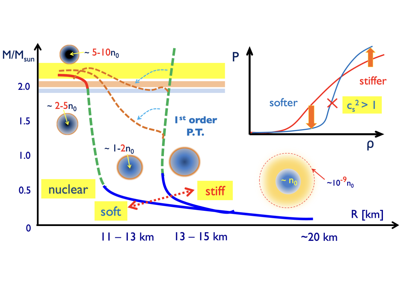
The most basic quantities in neutron star observations are the mass-radius ($M$-$R$) relations of neutron stars. As mentioned, the structure is determined by pressure v.s. energy density, $P(\rho)$, which enters Tolman-Oppenheimer-Volkoff (TOV) equation, a general relativistic version of the Newton equation for gravity,

$$\frac{dP(r)}{dr}=-\frac{GM(r)\rho(r)}{r^{2}}\bigg(1+\frac{\,P\,}{\rho}\bigg)\bigg(1+\frac{\,4\pi r^{3}P\,}{\,M(r)\,}\bigg)\bigg(1-\frac{\,2GM\,}{r}\bigg)^{-1}\,.$$

(1)

where the last three factors characterize the general relativistic effects, $P(r)$ and $\rho(r)$ are the pressure and density at the radial position, $r$ (Shapiro and Teukolsky 1983). The mass $M(r)$ inside of the radial coordinate $r$ is obtained by integrating the mass shell at $r$,

$$\frac{dM(r)}{dr}=4\pi r^{2}\rho(r)\,.$$

(2)

Actual computations begin with setting the central density $n_{c}$ at $r=0$ and then an equation of state is used to prepare $P$ and $\rho$ at given $n_{c}$. With these initial conditions and equations of state $P(\rho)$, the differential equations 1 and 2 are integrated until the pressure reaches zero, $P(r=R)=0$, which defines the radius $R$ of a neutron star. The neutron star mass is defined as $M(r=R)$. In this way, for a given central density $n_{c}$, one can obtain $M(R;n_{c})$. Repeating this procedure with changing $n_{c}$, one obtains the collection of such data forming a $M$-$R$ curve. There is one-to-one correspondence between $M$-$R$ curves and equations of state; in principle the equation of state can be directly extracted from observations. In reality there are only a few examples where $M$ and $R$ are determined simultaneously. In this situation some guides from theories should be supplemented.

From the center to the surface, the density drastically drops from $\sim 2-5n_{0}$ to $\sim 10^{-10}n_{0}$, and apparently it seems a formidable task to extract equations of state from such complex structure. Actually details of dilute matter do not have significant impacts on the $M$-$R$ relations, since dilute matter does not have large energy and its domain is highly compressed by the gravity; dilute matter with $n\ll n_{0}$ forms only a thin shell of $\sim 0.5$ km at most. A possible exception to this discussion is very light neutron stars with $M\sim 0.1-0.5M_{\odot}$ for which dilute matter is loosely compressed, but such neutron stars have not been discovered perhaps due to the absence of the formation process for such light neutron stars. With this considerations, one can concentrate on equations of state for $n\gtrsim 0.1n_{0}$ for discussions of $M$-$R$ curves. (The dilute matter part is crucial to discuss phenomena near the neutron star surfaces or finite temperature as the loosely bound matter is quite active.) (Page et al. 2006; Haensel et al. 2007)

It is very important to note that the shapes of $M$-$R$ curves are strongly correlated with the stiffness at several fiducial densities (Fig. 3). Stiff (soft) equations of state lead to larger (smaller) radii, and larger (smaller) maximum masses. From low mass to the mass $\sim 1.0M_{\odot}$, $M$-$R$ curves first show the shrinkage of $R$, and then radically changes the direction toward the vertical direction with small changes in $R$. This bending occurs with the central density around $\sim n_{0}$. This reflects that the compressed matter begins to observe repulsive forces in nuclear matter and matter can no longer be squeezed easily. The location of the bending sets the overall radius of neutron stars. Thus neutron star radii are typically sensitive to equations of state at $1-2n_{0}$ for wide range in $M$. The exceptions to this rule are equations of state with first order phase transitions; the associated radical softening induces kinks in $M$-$R$ curves, although up to now the signature of such kink structure has not been found for the interval $1.4-2.1M_{\odot}$. Beyond $\sim 1.4M_{\odot}$, the core density typically exceeds $2-3n_{0}$, entering the regime beyond purely nucleonic regime (see discussions below), and around $\sim 2M_{\odot}$, the density may reach $4-7n_{0}$. The existence of $2M_{\odot}$ neutron stars requires the high density matter at $4-7n_{0}$ to be very stiff.

In addition to observational constraints on $M$ and $R$, there are constraints on the interplay between low and high density equations of state. The first is the causality constraint, $dP/d\rho=c_{s}^{2}\leq 1$, which demands the sound velocity $c_{s}$ to be smaller than the light velocity. Another constraint is the thermodynamics stability, $d^{2}\rho/dn^{2}\geq 0$. For example, one cannot combine extremely soft low density equations of state and extremely stiff high density ones, since $dP/d\rho$ must grow too rapidly from low to high densities. With these constraints, it becomes theoretically more challenging if the maximum masses of neutron stars are larger and the radii are smaller than the currently available constraints. The low and high density equations of state constrain each other.

The following section starts with discussions of nuclear matter which have been studied intensively. Matter in neutron stars and supernovae are not isospin symmetric, so it is necessary to discuss equations of state as functions of density $n$ and proton fraction $Y_{p}$. The effects of temperatures are discussed for applications to supernova matter. These discussions are given for neutron stars with the masses up to $\sim 1.4M_{\odot}$ and the core densities up to $2-3n_{0}$. For $2M_{\odot}$ neutron stars, the core density is higher and more hypothetical arguments are needed. Discussions related to quark matter is postponed to the final part of this review.

In order to understand the conditions in astrophysical phenomena, it is helpful to recall the basic properties of ideal gas of electrons and nucleons (Lang 1980; Shapiro and Teukolsky 1983; Weiss et al. 2004). Simple relations of the thermodynamics for the degenerate gas of fermions provide the energy scale in neutron stars and nuclei. The number density of fermion gas is given by $n=gp_{F}^{3}/3\pi^{2}$ where $p_{F}$ is the Fermi momentum and $g$ is the number of degree of freedom for spin. For example, at the initial stage of supernovae, electrons in Fe cores with the number density $n$ and $Y_{p}=0.46$ have $p_{F}=10$ MeV $(n/10^{-5}~{\rm fm}^{-3})^{\frac{1}{3}}$ which is much greater than the electron mass $m_{e}\simeq 0.5$ MeV. Another characteristic scale is the nucleon Fermi momenta in symmetric matter ($Y_{p}=0.5$) which is evaluated to be $p_{F}=263$ MeV $(n/n_{0})^{\frac{1}{3}}$. The nucleons become relativistic when $p_{F}\simeq m_{N}$ or $n\simeq 50n_{0}$.

For a gas in the relativistic limit, the energy density scales as $\rho\propto p_{F}^{4}\propto n^{4/3}$. Using the relation $\mu=\partial\rho/\partial n$ ($\mu$: chemical potential) and the thermodynamic relation $P=\mu n-\rho$, one can write

$\displaystyle\rho_{\rm rela}(n)=cn^{4/3}~~\rightarrow~~P_{\rm rela}=\rho_{\rm rela}/3\,.$

(3)

This regime is relevant for electrons in Fe cores or neutron stars. Meanwhile, if fermions with the masses $m$ are non-relativistic ($m\gg p_{F}$), the energy density behaves as $\rho\sim c_{1}mn+c_{2}n^{5/3}/m$ with $c_{1},c_{2}$ being some constants. In this case

$\displaystyle\rho_{\rm NR}(n)=c_{1}mn+c_{2}\frac{\,n^{5/3}\,}{\,m\,}~~\rightarrow~~P_{\rm NR}=\frac{\,2\,}{\,3\,}c_{2}\frac{\,n^{5/3}\,}{\,m\,}~\propto~\rho_{\rm NR}^{5/3}m^{-8/3}\,.$

(4)

It is to be noted that the energy density $mn$ is much larger than the pressure; a non-relativistic gas is soft. In order for purely nucleonic descriptions to achieve a large neutron star mass of $\gtrsim M_{\odot}$, substantial repulsions among nucleons must be added to increase the pressure.

In order to parameterize the effects of interactions and the evolution from non-relativistic to relativistic regimes of dense matter, one often uses a polytrope form, $P=C\rho^{\Gamma}$, with $\Gamma$ called adiabatic index, and changes $\Gamma$ at some fiducial densities (Read et al. 2009). It has been known that a piecewide polytrope with the proper choice of $\Gamma$ and the fiducial densities can cover wide class of realistic equations of state.

The structure of neutron stars, especially the overall radii, is very sensitive to nuclear equations of state near the saturation density $n_{0}$ (Lattimer and Prakash 2001). Nuclear matter here is considered to be uniform and infinitely spread in space. The saturation density $n_{0}$ is close to the density inside of heavy nuclei, and one can infer the properties of nuclear matter from laboratory experiments for finite size nuclei. But the removal of finite size effects introduces uncertainties (Atkinson et al. 2020) which would change the neutron star radii by $\sim 0.5-1$ km; the pressure of nuclear matter is basically small, thus even small corrections from interactions affect the predictions for neutron stars. Hence, the precise determination of nuclear matter properties still remains an important problem. Below the basic properties of nuclear matter near saturation density are summarized. It is usually sufficient to evaluate contributions from nuclear interactions but neglecting the Coulomb energy among protons because the matter with leptons is locally charge neutral in most cases. The interactions among leptons are negligible and leptons can be added separately as an ideal gas.

Shown in Fig. 4 are typical behaviors of energies per nucleons with the mass subtracted, $\rho/n-m$, in symmetric matter ($Y_{p}=0.5$) and pure neutron matter ($Y_{p}=0$). In symmetric matter, there is a minimum at $n_{0}=0.16$ fm^-3 with $\rho/n-m\simeq-16$ MeV. This is called saturation point. Using the relation $P=\mu n-\rho=n^{2}\partial(\rho/n)/\partial n$, one can conclude the pressure at $n_{0}$ is zero; no external pressure is needed to maintain the finite matter, meaning that the matter is self-bound and stable against compression or expansion. This saturation property brings the stability of various nuclei at a constant density, and the density greater than $n_{0}$ is achieved only by substantial external pressure. Meanwhile, pure neutron matter is not self-bound. Thus neutron stars are bound by the gravitational forces which require macroscopic amount of materials as the source. Thus neutron stars cannot be arbitrarily light.

In applications to astrophysical phenomena, it is necessary to know the energy at various densities and proton fractions. The exploration to dense matter is often made by a simple form of the energy function, $E_{N}(n,Y_{p})=\rho/n-m$, as

$$E_{N}(n,Y_{p})=E_{N}(n_{0},Y_{p}=0.5)+\frac{K(Y_{p})}{18}\left(\frac{n-n_{0}}{n_{0}}\right)^{2}+S(n)(1-2Y_{p})^{2}+\cdots$$

(5)

in terms of the expansion around $n=n_{0}$ and $Y_{p}=0.5$. The coefficient $K(Y_{p})$ is called the incompressibility, the curvature at $n_{0}$ for a given $Y_{p}$. The coefficient $S(n)$ is called the symmetry energy which, in conventional literatures, is defined to be the second derivative of $E(n,Y_{p})$ with respect to $Y_{p}$ at $Y_{p}=0.5$. This definition does not directly coincide with $E(n,Y_{p}=0)-E(n,Y_{p}=0.5)$, but is chosen for the practical limitation that nuclear experiments cannot access the matter at $Y_{p}\sim 0$ where nuclei are unstable. In practice, available theoretical calculations suggest keeping only the leading order of the expansion, which starts with $(1-2Y_{p})^{2}$, is the good approximation around $n_{0}$. The symmetry energy near the nuclear density is expressed by $S(n)=S(n=n_{0})+\frac{L}{3n_{0}}(n-n_{0})$ using the slope parameter, $L$. These quantities are extracted to be $K(Y_{p}=0.5)=220-260$ MeV (Shlomo et al. 2006; Stone et al. 2014; Garg and Colò 2018), $S(n=n_{0})=24-36$ MeV, and $L=30-90$ MeV from the analyses of experimental data of nuclei for masses, radii and excitations (Tsang et al. 2012; Lattimer and Lim 2013; Horowitz et al. 2014; Özel and Freire 2016b; Li et al. 2018; Li et al. 2019). These uncertainties are converted into the uncertainties in overall neutron star radii with $\Delta R\sim 0.5-2$ km.

The direct calculations of infinite nuclear matter have played important roles in the neutron star context (Burgio et al. 2021). It can be applied to a matter with arbitrary $Y_{p}$, and especially pure neutron matter calculations are cleaner than symmetric matter due to fewer parameters in calculations. The most systematic approach is based on microscopic two- and three-nucleon forces which are constrained by nuclear two-body scattering below the pion production threshold, spectra of light nuclei, and a deuteron scattering off a proton that is sensitive to three-nucleon forces. Either traditional potential models (Stoks et al. 1994; Machleidt et al. 1996), which is based on the meson exchange picture, or chiral effective theory (Holt and Kaiser 2017; Drischler et al. 2021), which is based on momentum expansion, are used to characterize the nuclear forces (Machleidt and Sammarruca 2020). These nuclear forces are then used in many-body framework such as variational (Akmal et al. 1998; Togashi et al. 2017), quantum-Monte Carlo (Carlson et al. 2015), or many-body perturbation theories (Drischler et al. 2019). The modern calculations are consistent with the above-mentioned experimental estimates, but the pressure, which is sensitive to fine details, still has the uncertainties of $\sim 30$% at $n_{0}$ (see, e.g., Fig.1 in Kojo et al. 2021). These uncertainties grow with density, and in addition the validity to truncate many-body forces beyond three-body forces becomes questionable at $n\gtrsim 2n_{0}$. Thus a phenomenological modeling is often used beyond $n\sim 2n_{0}$ together with $2M_{\odot}$ constraints. Taking the microscopic calculations as the low density constraints, typical radii of $1.4M_{\odot}$ neutron stars are $11.5-13$ km.

The thermodynamic conditions in core-collapse supernovae and neutron star mergers vary over a wide range of density, temperature, and proton fraction. To construct data of the equations of state for the astrophysical simulations, phenomenological approaches are useful. The Skyrme-type interactions, which are represented as expansions of the effective interaction in powers of momenta and density-dependent three-body contributions, are the most well-known phenomenological modeling (Dutra et al. 2012). In the Skyrme-type models with the SLy4 parameters (Chabanat et al. 1998), the energy density of nuclear matteris expressed as

	$\displaystyle\rho(n,Y_{p},T)$	$\displaystyle=$	$\displaystyle\frac{\tau_{n}}{2m_{n}^{*}}+\frac{\tau_{p}}{2m_{p}^{*}}+\left(a+4bx(1-x)\right)n^{2}$		(6)
			$\displaystyle+\sum_{j=0,1,2}\left(c_{j}+4d_{j}x(1-x)\right)n^{1+\delta_{j}}+(1-x)nm_{n}+xnm_{p}\ ,$
	$\displaystyle\frac{1}{2m_{n}^{*}}$	$\displaystyle=$	$\displaystyle\frac{1}{2m_{n}}+\alpha_{1}n_{n}+\alpha_{2n_{p}}\ ,$		(7)
	$\displaystyle\frac{1}{2m_{p}^{*}}$	$\displaystyle=$	$\displaystyle\frac{1}{2m_{p}}+\alpha_{1}n_{p}+\alpha_{2n_{n}}\ ,$		(8)

where $a$, $b$, $c_{j}$, $d_{j}$, and $\delta_{j}$ are parameters of the Skyrme forces, $\tau_{n}$ and $\tau_{p}$ are the kinetic energy densities of neutrons and protons, respectively, and $m_{n}$ and $m_{p}$ are the masses of neutrons and protons, respectively. The first and second terms in Eq. (6) correspond to the non-relativistic kinetic energy densities of neutrons and protons, respectively. The third term represents two-nucleon interactions, and the summation over $j$ approximates the effects of many-body or density-dependent interactions. The last two terms in Eq. (6) express the rest masses of neutrons and protons, respectively. The parameters $\alpha_{1}$ and $\alpha_{2}$ for effective masses, $m_{n}^{*}$ and $m_{p}^{*}$, are chosen to reproduce observables of uniform nuclear matter together with $a$, $b$, $c_{j}$, $d_{j}$, and $\delta_{j}$.

Another phenomenological model of nuclear matter energy is the relativistic mean-field theory, in which nuclear interactions are described by the exchange of mesons. Up to this time, many parameter sets in the relativistic mean field theory have been adopted to construct equations of state for astrophysical simulations, e.g., DD2 (Typel et al. 2010), SFHx, and SFHo (Steiner et al. 2013). They are subject to constraints from terrestrial experiments and astrophysical observations (Stone 2021). For example, the Lagrangian with a parameter set TM1e (Shen et al. 2020) is ($M_{N}$: nucleon mass)

	$\displaystyle\mathcal{L}_{\rm{RMF}}$	$\displaystyle=$	$\displaystyle\sum_{i=p,n}\bar{\psi}_{i}\left[i\gamma_{\mu}\partial^{\mu}-\left(M_{N}+g_{\sigma}\sigma\right)\right.$		(9)
			$\displaystyle\left.-\gamma_{\mu}\left(g_{\omega}\omega^{\mu}+\frac{g_{\rho}}{2}\tau_{a}\rho^{a\mu}\right)\right]\psi_{i}$
			$\displaystyle+\frac{1}{2}\partial_{\mu}\sigma\partial^{\mu}\sigma-\frac{1}{2}m^{2}_{\sigma}\sigma^{2}-\frac{1}{3}g_{2}\sigma^{3}-\frac{1}{4}g_{3}\sigma^{4}$
			$\displaystyle-\frac{1}{4}W_{\mu\nu}W^{\mu\nu}+\frac{1}{2}m^{2}_{\omega}\omega_{\mu}\omega^{\mu}+\frac{1}{4}c_{3}\left(\omega_{\mu}\omega^{\mu}\right)^{2}$
			$\displaystyle-\frac{1}{4}R^{a}_{\mu\nu}R^{a\mu\nu}+\frac{1}{2}m^{2}_{\rho}\rho^{a}_{\mu}\rho^{a\mu}$
			$\displaystyle+\Lambda_{\rm{v}}\left(g_{\omega}^{2}\omega_{\mu}\omega^{\mu}\right)\left(g_{\rho}^{2}\rho^{a}_{\mu}\rho^{a\mu}\right),$

where $\psi$, $\sigma$, $\omega$, and $\rho$ denote nucleons, scalar-isoscalar mesons, vector-isoscalar mesons, and vector-isovector mesons, respectively, and $W_{\mu\nu}=\partial^{\mu}\omega^{\nu}-\partial^{\nu}\omega^{\mu}$ and $R^{a}_{\mu\nu}=\partial^{\mu}\rho^{a\nu}-\partial^{\nu}\rho^{a\mu}+g_{\rho}\epsilon^{abc}\rho^{b\mu}\rho^{c\nu}$. Nucleon-meson interactions are expressed as Yukawa couplings, and isoscalar mesons ($\sigma$ and $\omega$) interact with themselves. In the TM1e parameter set, the masses of mesons—$m_{\sigma}$, $m_{\omega}$, and $m_{\rho}$—and the coupling constants—$g_{\sigma}$, $g_{\omega}$, $g_{\rho}$, $g_{2}$, $g_{3}$,$c_{3}$, and $\Lambda_{\rm{v}}$—are determined to reproduce both properties of uniform nuclear matter at the saturation density (Oertel et al. 2017) and finite nuclei (Sugahara and Toki 1994; Bao and Shen 2014). In the mean field theory, mesons are assumed to be classical and are replaced by their ensemble averages. The Dirac equations for nucleons are quantized, and the free energies are evaluated based on their energy spectra. The meson fields and Dirac equations are self consistently solved (Sumiyoshi and Toki 1994).

For astrophysical applications, some microscopic models have been constructed with realistic interactions determined using the nucleon–nucleon scattering data. The variational method (Togashi and Takano 2013) for the Schrodinger’s equation are based on the realistic two-body nuclear potentials, which are adjusted to account for the data, and on a three-body potential. The Dirac Brückner Hartree–Fock theory (Katayama and Saito 2013) also employs the bare nuclear interactions. In contrast to variational method with a three-body potential, the Dirac Brückner Hartree–Fock theory reproduces nuclear saturation properties starting from two-body forces by solving the Bethe–Salpeter equation, single-particle self-energy, and the Dyson equation (Brockmann and Machleidt 1990).

In neutron star matter the charge neutrality and beta-equilibrium conditions introduce considerable asymmetry in the isospin density (Shapiro and Teukolsky 1983). The proton fraction is strongly correlated with the symmetry energy which characterizes the energy cost from the isospin asymmetry. Neutron star matter at $n_{0}$ has a small proton fraction of $Y_{p}\sim 0.1$, which is obtained by minimizing the total energy density, $\rho_{total}(n)=\rho(n,Y_{p})+\rho_{e}(n_{e})$, with respect to the proton fraction, where $\rho_{e}(n_{e})$ and $n_{e}=Y_{p}n$ are the electron energy density and number density. At higher density muons can also contribute. The condition at the minimum corresponds to the relation of the chemical equilibrium among particles, $\mu_{n}=\mu_{p}+\mu_{e}$, which states the balance of the Fermi energy of neutrons versus those of protons and electrons, $n\leftrightarrow p+e^{-}$, as shown in the left panel of Fig. 5. The set of these conditions is called as the beta equilibrium.

The composition and proton fraction change considerably from the surface to the core of a neutron star, where the density changes from $\sim 10^{-10}n_{0}$ to $\sim n_{0}$ as shown in Figs. 6 (Heiselberg 2002; Sumiyoshi 2018) and 7 (Chamel and Haensel 2008; Shen et al. 2020). Near the surface, nucleons form a nucleus and electrons are localized around it. The most stable nuclei are ⁵⁶Fe and the corresponding proton fraction is $Y_{p}\simeq 0.46$. This dilute regime begins to be modified beyond $10^{-8}n_{0}$, where it is energetically more favorable to reduce the number of electrons by the process $p+e^{-}\rightarrow n+\nu_{e}$. Accordingly the proton fraction decreases and a number of neutron rich nuclei, as indicated in the right panel of Fig. 7, appear . This region is called the outer crust (Chamel and Haensel 2008). Around $10^{-3}n_{0}$, there are too many neutrons and they begin to drip out of nuclei. The matter consists of nuclei, neutrons, and electrons in the region called the inner crust (Chamel and Haensel 2008). Further compression of nuclei to densities beyond $5\times 10^{-2}n_{0}$ merges them into the pasta structure, which has huge nuclei with various non-spherical shapes (Oyamatsu 1993). Above the nuclear density, $\sim 0.5n_{0}$, the nuclei are dissolved into neutrons and protons and the matter becomes uniform. In this regime the cost associated with the symmetry energy dominates over the cost of having electrons, thus $Y_{p}$ grows as density does.

Deep inside the central core at $n\gtrsim 2n_{0}$, there may be exotic phases with hyperons or quarks. Hyperons contain strange quarks. The appearance of these new particles is controlled by the condition of the chemical equilibrium. The chemical potential of neutrons, $\mu_{n}$, increases as the density goes up. When $\mu_{n}$ exceeds the mass of hyperons, $m_{\Lambda}$, for example, neutrons can be converted to hyperons because it reduces the Fermi energy of neutrons (right panel of Fig. 5). Allowing the appearance of new particles at a given density usually softens equations of state, as it increases the energy density by $\Delta\rho\sim mn$ but the associated increase in pressure is much smaller, $\Delta P\sim n^{5/3}/m$.

Shown in Fig. 8 are examples of $M$-$R$ curves for equations of state with and without hyperons, based on equations of state calculated in variational methods (Togashi et al. 2016). The maximum mass of $\sim 2.2M_{\odot}$ for purely nucleonic equations of state drops to $\sim 1.6M_{\odot}$ after including hyperons together with reasonable $YN$ forces. The small maximum mass incompatible with the $2M_{\odot}$ constraints suggests the necessity of some additional mechanisms. One possibility is the existence of strong $YNN$ repulsions that increase the density at which hyperons appear, as shown in Fig. 8. Clearly it is important to examine the properties of $YN$ and $YNN$ interactions (Vidaña 2018; Tolos and Fabbietti 2020). The experimental examination has difficulties since hyperons are unstable with respect to the weak decays and cannot be studied as in $NN$ scattering experiments. One possible way to study $YN$ interactions is to inject hadrons with strangeness into nuclei, create hyper nuclei, and then study the spectroscopy (Hiyama and Nakazawa 2018). Another method, which has been developed in last ten years, is to measure $YN$ interactions in lattice QCD (Iritani et al. 2019; Sasaki et al. 2020). The $YNN$ forces have not been determined yet.

The composition of matter is important not only for $M$-$R$ relations, but also for non-mechanical aspects of neutron stars, such as cooling curves or chemical reactions (Yakovlev and Pethick 2004; Page et al. 2004; Potekhin et al. 2015). The neutron stars cool down through the emission of neutrinos in dense matter, and its cooling rate strongly depends on the matter composition. The fastest cooling mechanism in $npe\mu$ matter is the direct Urca processes in which $n\rightarrow p+e^{-}+\bar{\nu}_{e}$ and $p+e^{-}\rightarrow n+\nu_{e}$ processes produce neutrinos escaping from the neutron star cores (Lattimer et al. 1991). The condition for these processes to occur is $Y_{p}\gtrsim 0.1$, as can be derived from the energy and momentum conservations. If this condition is not met, the modified Urca processes, $n+n\rightarrow n+p+e+\bar{\nu}_{e}$ and $n+p+e\rightarrow n+n+\nu_{e}$, are the next candidates for cooling mechanisms. The modified Urca is much slower than the direct one as the former requires two thermally excited nucleons, whose population are suppressed by the Boltzmann factor, to interact. Due to this large difference in cooling time scale for the $Y_{p}\gtrsim 0.1$ and $Y_{p}\lesssim 0.1$ cases, nuclear equations of state with the large symmetry energy can be differentiated from the others (Page and Applegate 1992). The complication is that typical nuclear equations of state lead to $Y_{p}\gtrsim 0.1$ only at sufficiently high densities where hyperons or quarks may appear. They open new channels for the fast cooling. Another important effect is the pairing gap which suppresses the abundance of thermally excited particles and thus neutrino production (Chamel and Haensel 2008). In what follows, the fast cooling requires sufficiently high density. The observed cooling curves seem to be consistent with the modified Urca, but it remains to be shown whether the core density reaches the density threshold for the direct Urca or not; for now the cooling curves and neutron star masses are not measured simultaneously.

The properties of hot and dense matter in core-collapse supernovae drastically change in the dynamical situations of collapse, bounce and explosion (Oertel et al. 2017). Typical conditions of the evolution of number density, temperature and electron fraction ($Y_{e}=Y_{p}$) at the center in the supernova core is shown in Fig. 9. The density and temperature increase rapidly in the collapse and reach high values at the core bounce. The electron fraction $Y_{e}$ decreases and remains $\sim 0.3$. It is useful to understand the time scale of changes of conditions and to examine the response of matter and neutrinos in the evolving environment.

The matter composed of nucleons, nuclei, electrons, positrons and photons is treated as a fluid component. The dynamical time scale, $T_{dyn}$, in fluid motion of free-fall under the gravitational force can be estimated to be $T_{dyn}\sim 5\times 10^{-3}\,{\rm s}\,(n/10^{-4}\,{\rm fm}^{-3})^{-1/2}$ (Shapiro and Teukolsky 1983). It takes $\sim 0.2-0.3$ s from the start of the gravitational collapse to the core bounce. This is much longer time scale than in strong and electro-magnetic interactions. Therefore, the nuclear and electro-magnetic processes can proceed fast enough to achieve the thermal and chemical equilibrium. Equations of state at a certain density, temperature, and electron fraction are necessary to perform numerical simulations.

Neutrinos are treated separately by solving the equations of neutrino transfer, which describes the propagation and reaction of neutrinos in matter. The time scale of weak reactions can be comparable or even longer than the dynamical time scale. For example, the time scale of the electron capture on free proton can be estimated to be $T_{e-cap}\sim 3\times 10^{2}~{\rm s}\,(n/10^{-6}~{\rm fm}^{-3})^{-5/3}(Y_{e}/0.46)^{-2/3}(X_{p}/10^{-4})^{-1}$ (Shapiro and Teukolsky 1983; Suzuki 1994) where $X_{p}$ is the mass fraction of free protons and the degenerate relativistic electron gas is assumed. It is not possible to assume the equilibrium for weak reactions, being different from the case of cold neutron stars. It is mandatory to follow the time evolution of the electron fraction of matter by tracking the modifications of composition through weak reactions. This requires detailed descriptions of neutrino reactions in matter as a source of changes. It is also necessary to provide the weak reaction rates, which largely depend on the target particles and environment of the matter.

At temperature of a few MeV achieved in supernova matter, fusing $N$ neutrons and $Z$ protons into a nuclide $(N,Z)$ is balanced by the photo-breakup reaction of the nuclide $(N,Z)$ into $N$ free neutrons and $Z$ free protons. In this nuclear statistical equilibrium, the compositions of nuclear matter (number densities of nucleons and all nuclei) are determined by minimizing the free energy of a model (Mazurek et al. 1979; Hempel and Schaffner-Bielich 2010). The free energy density of nuclear matter consists of contributions from nucleons and various nuclei as

$$f=f_{p}+f_{n}+\sum_{N,Z}f_{N}(N,Z),$$

(10)

where $f_{p}$ and $f_{n}$ are free energy densities of protons and neutrons, respectively. The free energy density of nuclei, $f_{N}(N,Z)$, is expressed as

$$f_{N}(N,Z)=n_{N}(N,Z)\{M(N,Z)+F_{t}(N,Z)\}$$

(11)

where $n_{N}(N,Z)$ represents the nuclear number density, $M(N,Z)$ represents nuclear mass and $F_{t}(N,Z)$ represents the free energy of translational motion.

The number densities of nuclei under the nuclear statistical equilibrium for the given $\rho$, $T$, and $Y_{p}$ are obtained by minimizing the model free energy with respect to the variational parameters. In the minimization the following mass and charge conservations are imposed,

$$n_{p}+n_{n}+\sum_{N,Z}{(N+Z)n_{N}}=n,$$

(12)

$$n_{p}+\sum_{N,Z}{Zn_{N}}=Y_{p}n,$$

(13)

where $n_{p}$ and $n_{n}$ are the number densities of free protons and neutrons, respectively. By introducing Lagrange multipliers $\alpha$ and $\beta$ for the above constraints, the free energy minimization as a function of $n_{p}$ and $n_{n}$ leads to ($i=p,n$)

$\displaystyle\frac{\partial}{\partial{n_{i}}}\bigg[f-\alpha\bigg(n_{p}+n_{n}+\sum_{N,Z}{(N+Z)n_{N}}-n\bigg)-\beta\bigg(n_{p}+\sum_{N,Z}{Zn_{N}}-Y_{p}n\bigg)\bigg]=0,$

(14)

Thus, the Lagrange multipliers are expressed with the chemical potentials of protons and neutrons, $\mu_{p}$ and $\mu_{n}$, as

	$\displaystyle\alpha$	$\displaystyle=$	$\displaystyle\frac{\partial f}{\partial n_{n}}=\mu_{n},$		(15)
	$\displaystyle\beta$	$\displaystyle=$	$\displaystyle\frac{\partial f}{\partial n_{p}}-\frac{\partial f}{\partial n_{n}}=\mu_{p}-\mu_{n}.$		(16)

The differentiation with respect to $n_{N}$, leads to the chemical potentials of nuclei, $\mu(N,Z)=\partial f/\partial n_{N}$, as

$$\mu(N,Z)=N\mu_{n}+Z\mu_{p}.$$

(17)

Here, nucleons and nuclei are treated as the ideal Boltzmann gases with their constant masses as

	$\displaystyle f(N,Z)$	$\displaystyle=$	$\displaystyle n_{N}(N,Z)\left[M(N,Z)+T\ln\left\{\frac{n_{N}(N,Z)}{g(N,Z)n_{Q}(N,Z)}\right\}-T\right],$		(18)
	$\displaystyle n_{Q}(N,Z)$	$\displaystyle=$	$\displaystyle\left(\frac{M(N,Z)k_{B}T}{2\pi}\right)^{3/2}.$		(19)

The partial differential of Eq. 18 with respect to $n_{N}(N,Z)$ and Eq. (17) lead to $n_{N}(N,Z)$ as follows:

$\displaystyle n_{N}(N,Z)=g(N,Z)\,n_{Q}(N,Z)\exp\left(\frac{Z\mu_{p}+N\mu_{n}-M(N,Z)}{T}\right),$

(20)

where $g(N,Z)$ is degeneracy factor of the nucleus. Calculations of $M(N,Z)$ depend on equations of state (Furusawa 2020).

Environment in supernovae evolves from a gravitationally collapsing massive star to the birth of a neutron star (Bethe 1990; Janka 2012; Oertel et al. 2017). The gravitational collapse starts from the central Fe core in the final stage of a massive star with the mass greater than $\sim 10M_{\odot}$. The central number density and temperature is typically $\sim 10^{-5}$ fm^-3 and $1$ MeV in the Fe core, which has a mass of $\sim 1.5M_{\odot}$ and radius of $\sim 10^{4}$ km, supported by pressure of electrons. The main composition is nuclei around ⁵⁶Fe which has a proton fraction, $Y_{p}=Z/A=26/56=0.46$, as the final product of nuclear fusion reactions to the most bound nuclei. Above the temperature $\sim 1$ MeV, the nuclear reactions among nucleons and nuclei proceed fast enough fast to maintain the nuclear statistical equilibrium.

The matter becomes neutron-rich in the collapse of the central core (Fig. 9 right). The electron captures proceed due to the high Fermi energy of electrons and the electron fraction decreases. The distribution of nuclei is shifted to the neutron-rich side, being away from the stability line. Fig. 10 displays the nuclei that are abundant during the collapse. The nuclear reactions during the collapse depend on the properties of neutron-rich nuclei and the associated response to electron captures.

At the initial stage, the neutrinos produced by the electron captures freely escape from the central core. They carry away the lepton number which is originally carried by electrons. As the electron captures proceed and neutrinos fly away, the electron fraction in the core decreases.

Further collapse of the central core, however, leads to higher densities of matter and the neutrino trapping due to the frequent scattering of neutrinos on nuclei. The neutrino transport eventually proceeds with the diffusion process. The time scale for the diffusion, $T_{diff}$, in the central core is estimated to be $T_{diff}\sim 4\times 10^{-2}~{\rm s}\,(n/10^{-4}~{\rm fm}^{-3})(A/56)$ based on the neutrino mean free path (Shapiro and Teukolsky 1983; Suzuki 1994). It becomes longer than the dynamical time scale, $T_{dyn}\sim 5\times 10^{-3}$ s at the density, $\rho=10^{-4}$ fm^-3 (Shapiro and Teukolsky 1983; Suzuki 1994). Therefore, the neutrinos cannot escape anymore and are trapped inside the central core beyond this density.

In matter compressed together with neutrinos, the trapped neutrinos can be treated as degenerate leptons. This state of matter is often called as the supernova matter, which is in thermal and chemical equilibrium. The supernova matter is parameterized by the lepton fraction, $Y_{L}$, instead of the electron fraction, $Y_{e}$. After the neutrino trapping, the lepton fraction remains constant during the gravitational collapse and after the core bounce (Fig. 9 right). The lepton fraction at this stage is important to determine the size of the bounce core to launch the shock wave.

Since there is no escape of particles to carry energy, the matter is compressed under the adiabatic condition. The entropy per baryon remains constant after the neutrino trapping during the gravitational collapse. The rise of the temperature is determined by the properties of the matter along the adiabatic curve. The temperature increases moderately even though the density increases dramatically (Fig. 9 middle).

The gravitational collapse with the neutrino trapping halts suddenly just above the nuclear density, $n_{0}$. The pressure abruptly increases above the nuclear density and the equation of state becomes stiff as shown in Fig. 11. This is mainly due to the repulsive contribution of nuclear forces. The adiabatic index, which corresponds to the slope of pressure versus density, becomes large $\sim 2$ above the value $\sim$4/3 for lepton gas during the collapse. This stiffening brings to a sudden stop of the compression of matter at the center and leads to bouncing back of the inner core. The shock wave is launched at the core bounce and starts propagating toward the outside as shown in Fig. 12. The central density is slightly above the nuclear density and the temperature is around $10-20$ MeV. The electron and lepton fractions are $\sim$0.29 and $\sim$0.35 due to the neutrino trapping with neutrino fraction $\sim$0.06 in this example. Note that the matter is not so neutron-rich having the proton fraction $\sim$0.29.

This is the starting point of the explosion although there are a number of obstacles to overcome. The initial position of the shock wave is located in the middle of the Fe core. The shock wave must reach the surface of the Fe core by propagating against the free-fall of matter of the outer part. It slows down also due to the loss of energy by the dissociation of Fe-group nuclei. The shock wave eventually stalls during the propagation inside the Fe core. This is the second stage of the explosion typically seen in many simulations, especially under the spherical symmetry, which leads to the failure of explosion.

In the current understanding of the explosion mechanism, it is considered that the neutrino heating mechanism assists the revival of the stalled shock wave (Bethe and Wilson 1985; Bethe 1990). The trapped neutrinos in the central part are gradually emitted to the outside and a part of outgoing neutrinos are absorbed by the material in the heating region just behind the stalled shock wave. The absorption of neutrinos heats the matter, increasing the internal energy and pressure to push the shock wave outwardly. The matter below the shock wave is composed of nucleons and light nuclei such as deuterons and $\alpha$ particles. Fig. 13 displays the mass fractions of the nuclei. The deuterons are abundant at $R\sim 10$–$50$ km above the surface of the proto-neutron star, while $\alpha$ particles are available at $R\sim 100$–$300$ km around and inside the shock wave. The nuclear matter that consists of nucleons and light nuclei also appear in heavy ion collisions and equations of state at low densities, $0.01n_{0}\lesssim n\lesssim 0.2n_{0}$, and may be experimentally constrained (Qin et al. 2012; Hempel et al. 2015).

The success of explosion requires an additional factor to raise the efficiency of the neutrino heating mechanism (Janka et al. 2012; Burrows 2013; Kotake 2013; Janka et al. 2016; Janka 2017a). In many of recent multi-dimensional simulations, the hydrodynamical instabilities assist the revival of the shock wave by giving an enough time for the neutrino heating. The convective motion, for example, brings the matter hovering in the heated region behind the shock wave to absorb enough neutrinos. The combination of the neutrino heating and the hydrodynamical instability is believed to be the major scenario of the explosion mechanism although the outcome of the (non-)explosion widely depends on the numerical simulations and microphysics.

Nuclear physics plays an important role to understand the initial stage of the shock wave during the collapse and bounce. The initial shock energy at the core bounce is estimated from the gravitational binding energy of the bounce core to be $E^{ini}_{shock}\sim GM^{2}_{bounce}/R_{bounce}$ where $M_{bounce}$ and $R_{bounce}$ is the mass and radius of the bounce core. The mass of the bounce core is determined by the Chandrasekhar mass, $M_{Ch}=1.5(Y_{L}/0.5)^{2}M_{\odot}$, supported by the pressure of leptons (Shapiro and Teukolsky 1983; Suzuki 1994). The lepton fraction, $Y_{L}$, is determined by the amount of electron captures and neutrino trapping during the collapse. The radius of the bounce core is determined by equations of state above the saturation density. For successful supernovae explosions, high compression of a matter and the associated quick increase in pressure is favored. Equations of state which are soft at low density meet such condition, but too soft ones are incompatible with the known properties of nuclei and neutron stars (Baron et al. 1985; Takahara and Sato 1988). There are also intriguing possibilities that a strong quark-hadron first order phase transition triggers the second bounce to launch the shock wave for the successful explosion (Fischer et al. 2011).

After the launch of shock waves, the nuclear physics is influential to the propagation of shock wave. One of the key factors is the mass of the bounce core; for a larger mass, the shock wave propagation is less disturbed by the energy loss associated with dissociation of the Fe nuclei (Janka et al. 2012). Another important physics is the neutrino energy at the emission region. Efficient heating of the shock waves favors energetic neutrino fluxes, which can be produced by high compression and high temperature as achieved by soft equations of state. Here the composition of matter is also very important, as the neutrino reactions strongly depend on target particles. Modeling of the nuclear statistical equilibrium and nuclear weak interactions has a significant impact on proto-neutron star masses and shock wave evolution to the same degree as the stiffness of the equation of state Nagakura et al. 2019b.

After the launch of shock waves, the central part of the core settles down to the quasi-hydrostatic configuration and the compact object is born at the center $\sim$0.3 s after the core bounce. It is called proto-neutron star which contains a plenty of neutrinos and anti-neutrinos of all three flavors (Burrows and Lattimer 1986; Suzuki 1994; Pons et al. 1999). Those neutrinos are produced by the weak reactions including the thermal processes such as the pair creation. It is also hot ($T\gtrsim 10$ MeV) and less neutron-rich ($Y_{e}\lesssim 0.3$) with a large radius $\sim 50$ km as compared to cold neutron stars as shown in the red lines in Fig. 14. The lepton fraction including neutrinos is determined during the collapse.

Proto-neutron stars cool down by emission of neutrinos. The temperature and electron fraction decrease since the neutrinos carry away the internal energy and lepton number as shown in Fig. 14. The evolution proceeds gradually over the time scale of $\sim 20$ s through the diffusion of neutrinos in the matter. The proto-neutron star becomes compact with radii $\lesssim 15$ km and the density becomes high. The proton fraction decreases to a small value, $Y_{p}\lesssim 0.1$, which is determined by the beta equilibrium without neutrinos. The proto-neutron star turns into a cold neutron star over the time scale of minutes.

The supernova neutrinos contain various information to probe inside the supernova core (Burrows 1988; Suzuki 1994; Janka 2017b; Müller 2019). The total energy of neutrinos can be used to derive the binding energy of the neutron star ($\sim 10^{53}$ erg). The average energy roughly reflects the temperature at the emission region. The time duration of neutrino emission is related with the diffusion time scale determined by the density. For example, soft equations of state lead to high energies of neutrinos and a long duration due to high density and temperature. Note that the neutrino emission is closely related with the explosion mechanism. The dynamics due to non-spherical motion of matter such as the convection and/or rotation leads to rapid variations of neutrino emission in time and, therefore, may be probed by neutrinos (Müller 2019). Observation of supernova neutrinos may provide the information on the properties of neutrinos through the phenomena of neutrino oscillations (Kotake et al. 2006; Duan and Kneller 2009; Mirizzi et al. 2016). The neutrinos may affect also the explosive nucleosynthesis, which takes place in the outer layers, by changing the composition (Woosley et al. 1990).

The supernova explosion is a target of the observation of gravitational waves, which brings the information of multi-dimensional dynamics (Kotake et al. 2006; Ott 2009; Kotake 2013). The time variation of the quadrupole moment of the matter distribution is a source of the variation of space-time metric in the Einstein equation of general relativity. The proto-neutron star is excited by fluid motions to have oscillations with the eigen frequencies of the gravitational wave (Ferrari et al. 2003; Sotani and Takiwaki 2016). Simultaneous detection of the neutrinos and gravitational waves from the nearby supernova will help to reveal the explosion dynamics in the era of the multi-messanger astronomy (Yokozawa et al. 2015).

The fate of the massive stars depends on the properties of the Fe core such as the compactness of density profile (Heger et al. 2003; O’Connor and Ott 2011). If the shock waves fail to revive, the accretion of matter continues and the mass of the proto-neutron star keeps growing. When it goes beyond the maximum mass supported by the supernova matter, the dynamical collapse occurs and a black hole is formed. A massive star fades away as a failed supernova (Kochanek et al. 2008; Adams et al. 2017). In Fig. 15, examples of the condition of matter in the evolution of supernova cores are shown. In the case of black hole formation, the density and temperature become very high and can be even beyond 100 MeV and $10$ fm^-3 due to the mass increase. The condition is more extreme than the case of proto-neutron star where the density stops growing at some point. This may open up possibilities of the appearance of the exotic particles such as hyperons and quarks. Note that the electron fraction is not so low (Fig. 15 right) due to the neutrino trapping, which tends to suppresses the appearance of exotic particles at the birth of proto-neutron star. Nevertheless, the evolution of density and temperature in the black hole formation can be extreme enough to yield hyperons and quarks.

Since the energy release of the accreting matter is efficient and the temperature becomes high, the luminosity and average energy of neutrinos increase rapidly toward the black hole formation. The typical duration of neutrino emission is $\sim 1$ s under the spherical symmetry. These features may be distinguished from the ordinary supernova neutrinos. They can be used to probe equations of state at extreme conditions (Sumiyoshi et al. 2006).

At very high density, quark matter descriptions should become more effective than hadronic ones. If one trusts quark matter descriptions down to the quark chemical potential $\mu_{c}$ such that $P(\mu=N_{c}\mu_{c})=0$, the corresponding baryon density, $n=n_{q}/N_{c}$, is nonzero,

$\displaystyle n_{c}=\frac{\,N_{f}\,}{\,3\pi^{2}\,}\mu_{c}^{3}\simeq 1.78n_{0}\times\bigg(\frac{\,N_{f}\,}{\,3\,}\bigg)^{1/4}\bigg(\frac{\,B^{1/4}\,}{\,146\,{\rm MeV}\,}\bigg)^{3}\,.$

(24)

The finite number density at zero pressure means that the matter is self-bound. A chunk of such a self-bound quark matter can form a quark star with the arbitrarily small mass. This should be contrasted to ordinary compact stars which require macroscopic amount of matter as a source of a strong gravity to trap neutron dominated matter (which is not self-bound). Witten calculated the $M$-$R$ relations for quark stars and found the scaling for the maximum mass and the corresponding radius (Witten 1984),

$\displaystyle M_{max}\simeq 2.0M_{\odot}\times\bigg(\frac{\,1.78n_{0}\,}{\,n_{c}\,}\bigg)^{2/3}\,,~~~~~~R|_{M_{max}}\simeq 10.7\,{\rm km}\times\frac{\,M_{\rm max}\,}{\,2M_{\odot}\,}\,,$

(25)

for $N_{f}=3$. The maximum mass can become arbitrarily large when $B$ or $n_{c}$ is reduced to smaller values. Thus, even without interactions, a relativistic quark gas can be very stiff, leading to a very large maximal mass. But the above estimate requires some precautions concerning the validity of pure quark matter descriptions. A small value of $B$ leads to a small density at $\mu_{c}$. Demanding the maximum mass of quark stars to be bigger than $2M_{\odot}$, the estimate $n_{c}<1.78n_{0}$ follows; presumably the matter is too dilute to entirely neglect the color confinement in QCD. Including the mass corrections makes the situation even worse by lowering $n_{c}$.

References

- Shapiro and Teukolsky (1983) S. L. Shapiro and S. A. Teukolsky, Black holes, white dwarfs, and neutron stars : the physics of compact objects (WILEY‐VCH Verlag GmbH and Co. KGaA, 1983).
- Hempel et al. (2015) M. Hempel, K. Hagel, J. Natowitz, G. Röpke, and S. Typel, Phys. Rev. C 91, 045805 (2015), arXiv:1503.00518 [nucl-th] .
- Oertel et al. (2017) M. Oertel, M. Hempel, T. Klähn, and S. Typel, Rev. Mod. Phys. 89, 015007 (2017), arXiv:1610.03361 [astro-ph.HE] .
- Haensel et al. (2007) P. Haensel, A. Y. Potekhin, and D. G. Yakovlev, Neutron Stars 1 : Equation of State and Structure, Vol. 326 (2007).
- Lorimer (2008) D. R. Lorimer, Living Reviews in Relativity 11, 8 (2008), arXiv:0811.0762 [astro-ph] .
- Lattimer (2012) J. M. Lattimer, Annual Review of Nuclear and Particle Science 62, 485 (2012), arXiv:1305.3510 [nucl-th] .
- Özel et al. (2012) F. Özel, D. Psaltis, R. Narayan, and A. Santos Villarreal, ApJ 757, 55 (2012), arXiv:1201.1006 [astro-ph.HE] .
- Kiziltan et al. (2013) B. Kiziltan, A. Kottas, M. De Yoreo, and S. E. Thorsett, ApJ 778, 66 (2013), arXiv:1011.4291 [astro-ph.GA] .
- Demorest et al. (2010) P. B. Demorest, T. Pennucci, S. M. Ransom, M. S. E. Roberts, and J. W. T. Hessels, Nature 467, 1081 (2010), arXiv:1010.5788 [astro-ph.HE] .
- Antoniadis et al. (2013) J. Antoniadis, P. C. C. Freire, N. Wex, T. M. Tauris, R. S. Lynch, M. H. van Kerkwijk, M. Kramer, C. Bassa, V. S. Dhillon, T. Driebe, J. W. T. Hessels, V. M. Kaspi, V. I. Kondratiev, N. Langer, T. R. Marsh, M. A. McLaughlin, T. T. Pennucci, S. M. Ransom, I. H. Stairs, J. van Leeuwen, J. P. W. Verbiest, and D. G. Whelan, Science 340, 448 (2013), arXiv:1304.6875 [astro-ph.HE] .
- Cromartie et al. (2020) H. T. Cromartie, E. Fonseca, S. M. Ransom, P. B. Demorest, Z. Arzoumanian, H. Blumer, P. R. Brook, M. E. DeCesar, T. Dolch, J. A. Ellis, R. D. Ferdman, E. C. Ferrara, N. Garver-Daniels, P. A. Gentile, M. L. Jones, M. T. Lam, D. R. Lorimer, R. S. Lynch, M. A. McLaughlin, C. Ng, D. J. Nice, T. T. Pennucci, R. Spiewak, I. H. Stairs, K. Stovall, J. K. Swiggum, and W. W. Zhu, Nature Astronomy 4, 72 (2020), arXiv:1904.06759 [astro-ph.HE] .
- Fonseca et al. (2021) E. Fonseca, H. T. Cromartie, T. T. Pennucci, P. S. Ray, A. Y. Kirichenko, S. M. Ransom, P. B. Demorest, I. H. Stairs, Z. Arzoumanian, L. Guillemot, A. Parthasarathy, M. Kerr, I. Cognard, P. T. Baker, H. Blumer, P. R. Brook, M. DeCesar, T. Dolch, F. A. Dong, E. C. Ferrara, W. Fiore, N. Garver-Daniels, D. C. Good, R. Jennings, M. L. Jones, V. M. Kaspi, M. T. Lam, D. R. Lorimer, J. Luo, A. McEwen, J. W. McKee, M. A. McLaughlin, N. McMann, B. W. Meyers, A. Naidu, C. Ng, D. J. Nice, N. Pol, H. A. Radovan, B. Shapiro-Albert, C. M. Tan, S. P. Tendulkar, J. K. Swiggum, H. M. Wahl, and W. W. Zhu, ApJ 915, L12 (2021), arXiv:2104.00880 [astro-ph.HE] .
- Fortin et al. (2015) M. Fortin, J. L. Zdunik, P. Haensel, and M. Bejger, A&A 576, A68 (2015), arXiv:1408.3052 [astro-ph.SR] .
- Özel and Freire (2016a) F. Özel and P. Freire, ARA&A 54, 401 (2016a), arXiv:1603.02698 [astro-ph.HE] .
- Watts et al. (2016) A. L. Watts et al., Rev. Mod. Phys. 88, 021001 (2016), arXiv:1602.01081 [astro-ph.HE] .
- Abbott et al. (2018) B. P. Abbott, R. Abbott, T. D. Abbott, F. Acernese, K. Ackley, C. Adams, T. Adams, P. Addesso, R. X. Adhikari, and V. B. Adya, Phys. Rev. Lett. 121, 161101 (2018), arXiv:1805.11581 [gr-qc] .
- Annala et al. (2018) E. Annala, T. Gorda, A. Kurkela, and A. Vuorinen, Phys. Rev. Lett. 120, 172703 (2018), arXiv:1711.02644 [astro-ph.HE] .
- Most et al. (2018) E. R. Most, L. R. Weih, L. Rezzolla, and J. Schaffner-Bielich, Phys. Rev. Lett. 120, 261103 (2018), arXiv:1803.00549 [gr-qc] .
- Miller et al. (2019) M. C. Miller, F. K. Lamb, A. J. Dittmann, S. Bogdanov, Z. Arzoumanian, K. C. Gendreau, S. Guillot, A. K. Harding, W. C. G. Ho, J. M. Lattimer, R. M. Ludlam, S. Mahmoodifar, S. M. Morsink, P. S. Ray, T. E. Strohmayer, K. S. Wood, T. Enoto, R. Foster, T. Okajima, G. Prigozhin, and Y. Soong, ApJ 887, L24 (2019), arXiv:1912.05705 [astro-ph.HE] .
- Riley et al. (2021) T. E. Riley, A. L. Watts, P. S. Ray, S. Bogdanov, S. Guillot, S. M. Morsink, A. V. Bilous, Z. Arzoumanian, D. Choudhury, J. S. Deneva, K. C. Gendreau, A. K. Harding, W. C. G. Ho, J. M. Lattimer, M. Loewenstein, R. M. Ludlam, C. B. Markwardt, T. Okajima, C. Prescod-Weinstein, R. A. Remillard, M. T. Wolff, E. Fonseca, H. T. Cromartie, M. Kerr, T. T. Pennucci, A. Parthasarathy, S. Ransom, I. Stairs, L. Guillemot, and I. Cognard, arXiv e-prints , arXiv:2105.06980 (2021), arXiv:2105.06980 [astro-ph.HE] .
- Miller et al. (2021) M. C. Miller, F. K. Lamb, A. J. Dittmann, S. Bogdanov, Z. Arzoumanian, K. C. Gendreau, S. Guillot, W. C. G. Ho, J. M. Lattimer, M. Loewenstein, S. M. Morsink, P. S. Ray, M. T. Wolff, C. L. Baker, T. Cazeau, S. Manthripragada, C. B. Markwardt, T. Okajima, S. Pollard, I. Cognard, H. T. Cromartie, E. Fonseca, L. Guillemot, M. Kerr, A. Parthasarathy, T. T. Pennucci, S. Ransom, and I. Stairs, arXiv e-prints , arXiv:2105.06979 (2021), arXiv:2105.06979 [astro-ph.HE] .
- Bethe (1990) H. A. Bethe, Reviews of Modern Physics 62, 801 (1990).
- Arnett (1996) D. Arnett, Supernovae and Nucleosynthesis: An Investigation of the History of Matter from the Big Bang to the Present (1996).
- Hirata et al. (1987) K. Hirata, T. Kajita, M. Koshiba, M. Nakahata, Y. Oyama, N. Sato, A. Suzuki, M. Takita, Y. Totsuka, T. Kifune, T. Suda, K. Takahashi, T. Tanimori, K. Miyano, M. Yamada, E. W. Beier, L. R. Feldscher, S. B. Kim, A. K. Mann, F. M. Newcomer, R. van, W. Zhang, and B. G. Cortez, Phys. Rev. Lett. 58, 1490 (1987).
- Bionta et al. (1987) R. M. Bionta, G. Blewitt, C. B. Bratton, D. Casper, A. Ciocio, R. Claus, B. Cortez, M. Crouch, S. T. Dye, S. Errede, G. W. Foster, W. Gajewski, K. S. Ganezer, M. Goldhaber, T. J. Haines, T. W. Jones, D. Kielczewska, W. R. Kropp, J. G. Learned, J. M. Losecco, J. Matthews, R. Miller, M. S. Mudan, H. S. Park, L. R. Price, F. Reines, J. Schultz, S. Seidel, E. Shumard, D. Sinclair, H. W. Sobel, J. L. Stone, L. R. Sulak, R. Svoboda, G. Thornton, J. C. van der Velde, and C. Wuest, Phys. Rev. Lett. 58, 1494 (1987).
- Sato and Suzuki (1987) K. Sato and H. Suzuki, Phys. Rev. Lett. 58, 2722 (1987).
- Burrows (1988) A. Burrows, ApJ 334, 891 (1988).
- Suzuki (1994) H. Suzuki, in Physics and Astrophysics of Neutrinos, edited by M. Fukugita and A. Suzuki (Springer-Verlag, Tokyo, 1994) p. 763.
- Scholberg (2012) K. Scholberg, Annual Review of Nuclear and Particle Science 62, 81 (2012), arXiv:1205.6003 [astro-ph.IM] .
- Hyper-Kamiokande Proto-Collaboration et al. (2018) Hyper-Kamiokande Proto-Collaboration, :, K. Abe, K. Abe, H. Aihara, A. Aimi, R. Akutsu, C. Andreopoulos, I. Anghel, L. H. V. Anthony, M. Antonova, Y. Ashida, V. Aushev, M. Barbi, G. J. Barker, G. Barr, P. Beltrame, V. Berardi, M. Bergevin, S. Berkman, L. Berns, T. Berry, S. Bhadra, D. Bravo-Berguño, F. d. M. Blaszczyk, A. Blondel, S. Bolognesi, S. B. Boyd, A. Bravar, C. Bronner, M. Buizza Avanzini, F. S. Cafagna, A. Cole, R. Calland, S. Cao, S. L. Cartwright, M. G. Catanesi, C. Checchia, Z. Chen-Wishart, J. H. Choi, K. Choi, J. Coleman, G. Collazuol, G. Cowan, L. Cremonesi, T. Dealtry, G. De Rosa, C. Densham, D. Dewhurst, E. L. Drakopoulou, F. Di Lodovico, O. Drapier, J. Dumarchez, P. Dunne, M. Dziewiecki, S. Emery, A. Esmaili, A. Evangelisti, E. Fernandez-Martinez, T. Feusels, A. Finch, A. Fiorentini, G. Fiorillo, M. Fitton, K. Frankiewicz, M. Friend, Y. Fujii, Y. Fukuda, D. Fukuda, K. Ganezer, C. Giganti, M. Gonin, N. Grant, P. Gumplinger, D. R. Hadley, B. Hartfiel, M. Hartz, Y. Hayato, K. Hayrapetyan, J. Hill, S. Hirota, S. Horiuchi, A. K. Ichikawa, T. Iijima, M. Ikeda, J. Imber, K. Inoue, J. Insler, R. A. Intonti, A. Ioannisian, T. Ishida, H. Ishino, M. Ishitsuka, Y. Itow, K. Iwamoto, A. Izmaylov, B. Jamieson, H. I. Jang, J. S. Jang, S. H. Jeon, M. Jiang, P. Jonsson, K. K. Joo, A. Kaboth, C. Kachulis, T. Kajita, J. Kameda, Y. Kataoka, T. Katori, K. Kayrapetyan, E. Kearns, M. Khabibullin, A. Khotjantsev, J. H. Kim, J. Y. Kim, S. B. Kim, S. Y. Kim, S. King, Y. Kishimoto, T. Kobayashi, M. Koga, A. Konaka, L. L. Kormos, Y. Koshio, A. Korzenev, K. L. Kowalik, W. R. Kropp, Y. Kudenko, R. Kurjata, T. Kutter, M. Kuze, L. Labarga, J. Lagoda, P. J. J. Lasorak, M. Laveder, M. Lawe, J. G. Learned, I. T. Lim, T. Lindner, R. P. Litchfield, A. Longhin, P. Loverre, T. Lou, L. Ludovici, W. Ma, L. Magaletti, K. Mahn, M. Malek, L. Maret, C. Mariani, K. Martens, L. Marti, J. F. Martin, J. Marzec, S. Matsuno, E. Mazzucato, M. McCarthy, N. McCauley, K. S. McFarland, C. McGrew, A. Mefodiev, P. Mermod, C. Metelko, M. Mezzetto, J. Migenda, P. Mijakowski, H. Minakata, A. Minamino, S. Mine, O. Mineev, A. Mitra, M. Miura, T. Mochizuki, J. Monroe, D. H. Moon, S. Moriyama, T. Mueller, F. Muheim, K. Murase, F. Muto, M. Nakahata, Y. Nakajima, K. Nakamura, T. Nakaya, S. Nakayama, C. Nantais, M. Needham, T. Nicholls, Y. Nishimura, E. Noah, F. Nova, J. Nowak, H. Nunokawa, Y. Obayashi, H. M. O’Keeffe, Y. Okajima, K. Okumura, Y. Onishchuk, E. O’Sullivan, L. O’Sullivan, T. Ovsiannikova, R. A. Owen, Y. Oyama, M. Y. Pac, V. Palladino, J. L. Palomino, V. Paolone, W. Parker, S. Parsa, D. Payne, J. D. Perkin, C. Pidcott, E. Pinzon Guerra, S. Playfer, B. Popov, M. Posiadala-Zezula, J. M. Poutissou, A. Pritchard, N. W. Prouse, G. Pronost, P. Przewlocki, B. Quilain, E. Radicioni, P. N. Ratoff, F. Retiere, C. Riccio, B. Richards, E. Rondio, H. J. Rose, C. Rott, S. D. Rountree, A. C. Ruggeri, A. Rychter, R. Sacco, M. Sakuda, M. C. Sanchez, E. Scantamburlo, M. Scott, S. M. Sedgwick, Y. Seiya, T. Sekiguchi, H. Sekiya, S. H. Seo, D. Sgalaberna, R. Shah, A. Shaikhiev, I. Shimizu, M. Shiozawa, Y. Shitov, S. Short, C. Simpson, G. Sinnis, M. B. Smy, S. Snow, J. Sobczyk, H. W. Sobel, Y. Sonoda, R. Spina, T. Stewart, J. L. Stone, Y. Suda, Y. Suwa, Y. Suzuki, A. T. Suzuki, R. Svoboda, M. Taani, R. Tacik, A. Takeda, A. Takenaka, A. Taketa, Y. Takeuchi, V. Takhistov, H. A. Tanaka, H. K. M. Tanaka, H. Tanaka, R. Terri, M. Thiesse, L. F. Thompson, M. Thorpe, S. Tobayama, C. Touramanis, T. Towstego, T. Tsukamoto, K. M. Tsui, M. Tzanov, Y. Uchida, M. R. Vagins, G. Vasseur, C. Vilela, R. B. Vogelaar, J. Walding, J. Walker, M. Ward, D. Wark, M. O. Wascko, A. Weber, R. Wendell, R. J. Wilkes, M. J. Wilking, J. R. Wilson, T. Xin, K. Yamamoto, C. Yanagisawa, T. Yano, S. Yen, N. Yershov, D. N. Yeum, M. Yokoyama, T. Yoshida, I. Yu, M. Yu, J. Zalipska, K. Zaremba, M. Ziembicki, M. Zito, and S. Zsoldos, arXiv e-prints , arXiv:1805.04163 (2018), arXiv:1805.04163 [physics.ins-det] .
- Suwa et al. (2019) Y. Suwa, K. Sumiyoshi, K. Nakazato, Y. Takahira, Y. Koshio, M. Mori, and R. A. Wendell, ApJ 881, 139 (2019), arXiv:1904.09996 [astro-ph.HE] .
- Kotake et al. (2006) K. Kotake, K. Sato, and K. Takahashi, Reports on Progress in Physics 69, 971 (2006), arXiv:astro-ph/0509456 [astro-ph] .
- Ott (2009) C. D. Ott, Classical and Quantum Gravity 26, 063001 (2009), arXiv:0809.0695 [astro-ph] .
- Kotake (2013) K. Kotake, Comptes Rendus Physique 14, 318 (2013), arXiv:1110.5107 [astro-ph.HE] .
- Ando et al. (2005) S. Ando, J. F. Beacom, and H. Yüksel, Phys. Rev. Lett. 95, 171101 (2005), arXiv:astro-ph/0503321 [astro-ph] .
- Horiuchi et al. (2009) S. Horiuchi, J. F. Beacom, and E. Dwek, Phys. Rev. D 79, 083013 (2009), arXiv:0812.3157 [astro-ph] .
- Page et al. (2006) D. Page, U. Geppert, and F. Weber, Nucl. Phys. A 777, 497 (2006), arXiv:astro-ph/0508056 [astro-ph] .
- Lang (1980) K. R. Lang, Astrophysical Formulae. A Compendium for the Physicist and Astrophysicist., second corrected and enlarged edition ed. (Springer-Verlag, Berlin Heidelberg New York, 1980).
- Weiss et al. (2004) A. Weiss, W. Hillebrandt, H. C. Thomas, and H. Ritter, Cox and Giuli’s Principles of Stellar Structure (Cambridge Scientific Publishers, 2004).
- Read et al. (2009) J. S. Read, B. D. Lackey, B. J. Owen, and J. L. Friedman, Phys. Rev. D 79, 124032 (2009), arXiv:0812.2163 [astro-ph] .
- Lattimer and Prakash (2001) J. M. Lattimer and M. Prakash, Astrophys. J. 550, 426 (2001), arXiv:astro-ph/0002232 .
- Atkinson et al. (2020) M. C. Atkinson, W. H. Dickhoff, M. Piarulli, A. Rios, and R. B. Wiringa, Phys. Rev. C 102, 044333 (2020), arXiv:2001.07231 [nucl-th] .
- Shlomo et al. (2006) S. Shlomo, V. M. Kolomietz, and G. Colò, European Physical Journal A 30, 23 (2006).
- Stone et al. (2014) J. R. Stone, N. J. Stone, and S. A. Moszkowski, Phys. Rev. C 89, 044316 (2014), arXiv:1404.0744 [nucl-th] .
- Garg and Colò (2018) U. Garg and G. Colò, Progress in Particle and Nuclear Physics 101, 55 (2018), arXiv:1801.03672 [nucl-ex] .
- Tsang et al. (2012) M. B. Tsang, J. R. Stone, F. Camera, P. Danielewicz, S. Gandolfi, K. Hebeler, C. J. Horowitz, J. Lee, W. G. Lynch, Z. Kohley, R. Lemmon, P. Möller, T. Murakami, S. Riordan, X. Roca-Maza, F. Sammarruca, A. W. Steiner, I. Vidaña, and S. J. Yennello, Phys. Rev. C 86, 015803 (2012), arXiv:1204.0466 [nucl-ex] .
- Lattimer and Lim (2013) J. M. Lattimer and Y. Lim, ApJ 771, 51 (2013), arXiv:1203.4286 [nucl-th] .
- Horowitz et al. (2014) C. J. Horowitz, E. F. Brown, Y. Kim, W. G. Lynch, R. Michaels, A. Ono, J. Piekarewicz, M. B. Tsang, and H. H. Wolter, Journal of Physics G Nuclear Physics 41, 093001 (2014), arXiv:1401.5839 [nucl-th] .
- Özel and Freire (2016b) F. Özel and P. Freire, ARA&A 54, 401 (2016b), arXiv:1603.02698 [astro-ph.HE] .
- Li et al. (2018) B.-A. Li, B.-J. Cai, L.-W. Chen, and J. Xu, Progress in Particle and Nuclear Physics 99, 29 (2018), arXiv:1801.01213 [nucl-th] .
- Li et al. (2019) B.-A. Li, P. G. Krastev, D.-H. Wen, and N.-B. Zhang, European Physical Journal A 55, 117 (2019), arXiv:1905.13175 [nucl-th] .
- Burgio et al. (2021) G. F. Burgio, H. J. Schulze, I. Vidaña, and J. B. Wei, Progress in Particle and Nuclear Physics 120, 103879 (2021), arXiv:2105.03747 [nucl-th] .
- Stoks et al. (1994) V. G. J. Stoks, R. A. M. Klomp, C. P. F. Terheggen, and J. J. de Swart, Phys. Rev. C 49, 2950 (1994), arXiv:nucl-th/9406039 .
- Machleidt et al. (1996) R. Machleidt, F. Sammarruca, and Y. Song, Phys. Rev. C 53, R1483 (1996), arXiv:nucl-th/9510023 .
- Holt and Kaiser (2017) J. W. Holt and N. Kaiser, Phys. Rev. C 95, 034326 (2017).
- Drischler et al. (2021) C. Drischler, J. W. Holt, and C. Wellenhofer, arXiv e-prints , arXiv:2101.01709 (2021), arXiv:2101.01709 [nucl-th] .
- Machleidt and Sammarruca (2020) R. Machleidt and F. Sammarruca, Eur. Phys. J. A 56, 95 (2020), arXiv:2001.05615 [nucl-th] .
- Akmal et al. (1998) A. Akmal, V. R. Pandharipande, and D. G. Ravenhall, Phys. Rev. C 58, 1804 (1998), arXiv:nucl-th/9804027 .
- Togashi et al. (2017) H. Togashi, K. Nakazato, Y. Takehara, S. Yamamuro, H. Suzuki, and M. Takano, Nucl. Phys. A 961, 78 (2017), arXiv:1702.05324 [nucl-th] .
- Carlson et al. (2015) J. Carlson, S. Gandolfi, F. Pederiva, S. C. Pieper, R. Schiavilla, K. E. Schmidt, and R. B. Wiringa, Rev. Mod. Phys. 87, 1067 (2015), arXiv:1412.3081 [nucl-th] .
- Drischler et al. (2019) C. Drischler, K. Hebeler, and A. Schwenk, Phys. Rev. Lett. 122, 042501 (2019), arXiv:1710.08220 [nucl-th] .
- Kojo et al. (2021) T. Kojo, G. Baym, and T. Hatsuda, (2021), arXiv:2111.11919 [astro-ph.HE] .
- Dutra et al. (2012) M. Dutra, O. Lourenco, J. S. Sa Martins, A. Delfino, J. R. Stone, and P. D. Stevenson, Phys. Rev. C 85, 035201 (2012).
- Chabanat et al. (1998) E. Chabanat, P. Bonche, P. Haensel, J. Meyer, and R. Schaeffer, Nuclear Physics A 635, 231 (1998).
- Typel et al. (2010) S. Typel, G. Röpke, T. Klähn, D. Blaschke, and H. H. Wolter, Phys. Rev. C 81, 015803 (2010), arXiv:0908.2344 [nucl-th] .
- Steiner et al. (2013) A. W. Steiner, M. Hempel, and T. Fischer, ApJ 774, 17 (2013), arXiv:1207.2184 [astro-ph.SR] .
- Stone (2021) J. R. Stone, Universe 7, 257 (2021).
- Shen et al. (2020) H. Shen, F. Ji, J. Hu, and K. Sumiyoshi, ApJ 891, 148 (2020), arXiv:2001.10143 [nucl-th] .
- Oertel et al. (2017) M. Oertel, M. Hempel, T. Klähn, and S. Typel, Reviews of Modern Physics 89, 015007 (2017), arXiv:1610.03361 [astro-ph.HE] .
- Sugahara and Toki (1994) Y. Sugahara and H. Toki, Nucl. Phys. A 579, 557 (1994).
- Bao and Shen (2014) S. S. Bao and H. Shen, Phys. Rev. C 89, 045807 (2014), arXiv:1405.3837 [nucl-th] .
- Sumiyoshi and Toki (1994) K. Sumiyoshi and H. Toki, ApJ 422, 700 (1994).
- Togashi and Takano (2013) H. Togashi and M. Takano, Nucl. Phys. A 902, 53 (2013), arXiv:1302.4261 [nucl-th] .
- Katayama and Saito (2013) T. Katayama and K. Saito, Phys. Rev. C 88, 035805 (2013), arXiv:1307.2067 [nucl-th] .
- Brockmann and Machleidt (1990) R. Brockmann and R. Machleidt, Phys. Rev. C 42, 1965 (1990).
- Sumiyoshi (2018) K. Sumiyoshi, The puzzle of supernova explosions unraveled by nuclear physics (Kyoritsu Shuppan Co., Ltd., 2018).
- Heiselberg (2002) H. Heiselberg, arXiv e-prints , astro-ph/0201465 (2002), arXiv:astro-ph/0201465 [astro-ph] .
- Chamel and Haensel (2008) N. Chamel and P. Haensel, Living Reviews in Relativity 11, 10 (2008), arXiv:0812.3955 [astro-ph] .
- Oyamatsu (1993) K. Oyamatsu, Nucl. Phys. A 561, 431 (1993).
- Togashi et al. (2016) H. Togashi, E. Hiyama, Y. Yamamoto, and M. Takano, Phys. Rev. C 93, 035808 (2016), arXiv:1602.08106 [nucl-th] .
- Vidaña (2018) I. Vidaña, Proceedings of the Royal Society of London Series A 474, 20180145 (2018), arXiv:1803.00504 [nucl-th] .
- Tolos and Fabbietti (2020) L. Tolos and L. Fabbietti, Progress in Particle and Nuclear Physics 112, 103770 (2020), arXiv:2002.09223 [nucl-ex] .
- Hiyama and Nakazawa (2018) E. Hiyama and K. Nakazawa, Ann. Rev. Nucl. Part. Sci. 68, 131 (2018).
- Iritani et al. (2019) T. Iritani et al. (HAL QCD), Phys. Lett. B 792, 284 (2019), arXiv:1810.03416 [hep-lat] .
- Sasaki et al. (2020) K. Sasaki et al. (HAL QCD), Nucl. Phys. A 998, 121737 (2020), arXiv:1912.08630 [hep-lat] .
- Yakovlev and Pethick (2004) D. G. Yakovlev and C. J. Pethick, ARA&A 42, 169 (2004), arXiv:astro-ph/0402143 [astro-ph] .
- Page et al. (2004) D. Page, J. M. Lattimer, M. Prakash, and A. W. Steiner, ApJS 155, 623 (2004), arXiv:astro-ph/0403657 [astro-ph] .
- Potekhin et al. (2015) A. Y. Potekhin, J. A. Pons, and D. Page, Space Sci. Rev. 191, 239 (2015), arXiv:1507.06186 [astro-ph.HE] .
- Lattimer et al. (1991) J. M. Lattimer, C. J. Pethick, M. Prakash, and P. Haensel, Phys. Rev. Lett. 66, 2701 (1991).
- Page and Applegate (1992) D. Page and J. H. Applegate, ApJ 394, L17 (1992).
- Furusawa et al. (2017a) S. Furusawa, H. Togashi, H. Nagakura, K. Sumiyoshi, S. Yamada, H. Suzuki, and M. Takano, Journal of Physics G Nuclear Physics 44, 094001 (2017a), arXiv:1707.06410 [astro-ph.HE] .
- Nakazato et al. (2021) K. Nakazato, K. Sumiyoshi, and H. Togashi, PASJ 73, 639 (2021), arXiv:2103.14386 [astro-ph.HE] .
- Mazurek et al. (1979) T. J. Mazurek, G. E. Brown, and J. M. Lattimer, ApJ 229, 713 (1979).
- Hempel and Schaffner-Bielich (2010) M. Hempel and J. Schaffner-Bielich, Nucl. Phys. A 837, 210 (2010), arXiv:0911.4073 [nucl-th] .
- Furusawa (2020) S. Furusawa, Phys. Scr 95, 074002 (2020).
- Janka (2012) H.-T. Janka, Annual Review of Nuclear and Particle Science 62, 407 (2012), arXiv:1206.2503 [astro-ph.SR] .
- Furusawa et al. (2017b) S. Furusawa, H. Nagakura, K. Sumiyoshi, C. Kato, and S. Yamada, Phys. Rev. C 95, 025809 (2017b), arXiv:1701.08414 [astro-ph.HE] .
- Bethe and Wilson (1985) H. A. Bethe and J. R. Wilson, ApJ 295, 14 (1985).
- Qin et al. (2012) L. Qin, K. Hagel, R. Wada, J. B. Natowitz, S. Shlomo, A. Bonasera, G. Röpke, S. Typel, Z. Chen, M. Huang, J. Wang, H. Zheng, S. Kowalski, M. Barbui, M. R. D. Rodrigues, K. Schmidt, D. Fabris, M. Lunardon, S. Moretto, G. Nebbia, S. Pesente, V. Rizzi, G. Viesti, M. Cinausero, G. Prete, T. Keutgen, Y. El Masri, Z. Majka, and Y. G. Ma, Phys. Rev. Lett. 108, 172701 (2012).
- Nagakura et al. (2019a) H. Nagakura, K. Sumiyoshi, and S. Yamada, ApJ 880, L28 (2019a), arXiv:1907.04863 [astro-ph.HE] .
- Janka et al. (2012) H.-T. Janka, F. Hanke, L. Hüdepohl, A. Marek, B. Müller, and M. Obergaulinger, Progress of Theoretical and Experimental Physics 2012, 01A309 (2012), arXiv:1211.1378 [astro-ph.SR] .
- Burrows (2013) A. Burrows, Reviews of Modern Physics 85, 245 (2013), arXiv:1210.4921 [astro-ph.SR] .
- Janka et al. (2016) H.-T. Janka, T. Melson, and A. Summa, Annual Review of Nuclear and Particle Science 66, 341 (2016), arXiv:1602.05576 [astro-ph.SR] .
- Janka (2017a) H.-T. Janka, “Neutrino-Driven Explosions,” in Handbook of Supernovae, ISBN 978-3-319-21845-8. Springer International Publishing AG, 2017, p. 1095 (Springer, 2017) p. 1095.
- Baron et al. (1985) E. Baron, J. Cooperstein, and S. Kahana, Phys. Rev. Lett. 55, 126 (1985).
- Takahara and Sato (1988) M. Takahara and K. Sato, ApJ 335, 301 (1988).
- Fischer et al. (2011) T. Fischer, I. Sagert, G. Pagliara, M. Hempel, J. Schaffner-Bielich, T. Rauscher, F. K. Thielemann, R. Käppeli, G. Martínez-Pinedo, and M. Liebendörfer, ApJS 194, 39 (2011), arXiv:1011.3409 [astro-ph.HE] .
- Nagakura et al. (2019b) H. Nagakura, S. Furusawa, H. Togashi, S. Richers, K. Sumiyoshi, and S. Yamada, ApJS 240, 38 (2019b), arXiv:1812.09811 [astro-ph.HE] .
- Burrows and Lattimer (1986) A. Burrows and J. M. Lattimer, ApJ 307, 178 (1986).
- Pons et al. (1999) J. A. Pons, S. Reddy, M. Prakash, J. M. Lattimer, and J. A. Miralles, ApJ 513, 780 (1999), arXiv:astro-ph/9807040 [astro-ph] .
- Janka (2017b) H.-T. Janka, “Neutrino Emission from Supernovae,” in Handbook of Supernovae, ISBN 978-3-319-21845-8. Springer International Publishing AG, 2017, p. 1575 (Springer, 2017) p. 1575.
- Müller (2019) B. Müller, Annual Review of Nuclear and Particle Science 69, 253 (2019), arXiv:1904.11067 [astro-ph.HE] .
- Duan and Kneller (2009) H. Duan and J. P. Kneller, Journal of Physics G Nuclear Physics 36, 113201 (2009), arXiv:0904.0974 [astro-ph.HE] .
- Mirizzi et al. (2016) A. Mirizzi, I. Tamborra, H. T. Janka, N. Saviano, K. Scholberg, R. Bollig, L. Hüdepohl, and S. Chakraborty, Nuovo Cimento Rivista Serie 39, 1 (2016), arXiv:1508.00785 [astro-ph.HE] .
- Woosley et al. (1990) S. E. Woosley, D. H. Hartmann, R. D. Hoffman, and W. C. Haxton, ApJ 356, 272 (1990).
- Ferrari et al. (2003) V. Ferrari, G. Miniutti, and J. A. Pons, MNRAS 342, 629 (2003), arXiv:astro-ph/0210581 [astro-ph] .
- Sotani and Takiwaki (2016) H. Sotani and T. Takiwaki, Phys. Rev. D 94, 044043 (2016), arXiv:1608.01048 [astro-ph.HE] .
- Yokozawa et al. (2015) T. Yokozawa, M. Asano, T. Kayano, Y. Suwa, N. Kanda, Y. Koshio, and M. R. Vagins, Astrophys. J. 811, 86 (2015).
- Heger et al. (2003) A. Heger, C. L. Fryer, S. E. Woosley, N. Langer, and D. H. Hartmann, ApJ 591, 288 (2003), arXiv:astro-ph/0212469 [astro-ph] .
- O’Connor and Ott (2011) E. O’Connor and C. D. Ott, ApJ 730, 70 (2011), arXiv:1010.5550 [astro-ph.HE] .
- Kochanek et al. (2008) C. S. Kochanek, J. F. Beacom, M. D. Kistler, J. L. Prieto, K. Z. Stanek, T. A. Thompson, and H. Yüksel, ApJ 684, 1336 (2008), arXiv:0802.0456 [astro-ph] .
- Adams et al. (2017) S. M. Adams, C. S. Kochanek, J. R. Gerke, K. Z. Stanek, and X. Dai, MNRAS 468, 4968 (2017), arXiv:1609.01283 [astro-ph.SR] .
- Sumiyoshi et al. (2019) K. Sumiyoshi, K. Nakazato, H. Suzuki, J. Hu, and H. Shen, ApJ 887, 110 (2019), arXiv:1908.02928 [astro-ph.HE] .
- Sumiyoshi (2017) K. Sumiyoshi, in Journal of Physics Conference Series, Journal of Physics Conference Series, Vol. 861 (2017) p. 012028.
- Sumiyoshi et al. (2006) K. Sumiyoshi, S. Yamada, H. Suzuki, and S. Chiba, Phys. Rev. Lett. 97, 091101 (2006), arXiv:astro-ph/0608509 [astro-ph] .
- Fujibayashi et al. (2017) S. Fujibayashi, Y. Sekiguchi, K. Kiuchi, and M. Shibata, ApJ 846, 114 (2017), arXiv:1703.10191 [astro-ph.HE] .
- Sumiyoshi et al. (2021) K. Sumiyoshi, S. Fujibayashi, Y. Sekiguchi, and M. Shibata, ApJ 907, 92 (2021), arXiv:2010.10865 [astro-ph.HE] .
- Abbott et al. (2017) B. P. Abbott et al. (LIGO Scientific, Virgo), Phys. Rev. Lett. 119, 161101 (2017), arXiv:1710.05832 [gr-qc] .
- Hinderer et al. (2010) T. Hinderer, B. D. Lackey, R. N. Lang, and J. S. Read, Phys. Rev. D 81, 123016 (2010), arXiv:0911.3535 [astro-ph.HE] .
- Ravi and Lasky (2014) V. Ravi and P. D. Lasky, Mon. Not. Roy. Astron. Soc. 441, 2433 (2014), arXiv:1403.6327 [astro-ph.HE] .
- Shibata and Hotokezaka (2019) M. Shibata and K. Hotokezaka, Ann. Rev. Nucl. Part. Sci. 69, 41 (2019), arXiv:1908.02350 [astro-ph.HE] .
- Kasen et al. (2017) D. Kasen, B. Metzger, J. Barnes, E. Quataert, and E. Ramirez-Ruiz, Nature 551, 80 (2017), arXiv:1710.05463 [astro-ph.HE] .
- Bauswein et al. (2017) A. Bauswein, O. Just, H.-T. Janka, and N. Stergioulas, Astrophys. J. Lett. 850, L34 (2017), arXiv:1710.06843 [astro-ph.HE] .
- Radice and Dai (2019) D. Radice and L. Dai, Eur. Phys. J. A 55, 50 (2019), arXiv:1810.12917 [astro-ph.HE] .
- Breu and Rezzolla (2016) C. Breu and L. Rezzolla, Mon. Not. Roy. Astron. Soc. 459, 646 (2016), arXiv:1601.06083 [gr-qc] .
- Baiotti and Rezzolla (2017) L. Baiotti and L. Rezzolla, Rept. Prog. Phys. 80, 096901 (2017), arXiv:1607.03540 [gr-qc] .
- Margalit and Metzger (2017) B. Margalit and B. D. Metzger, Astrophys. J. Lett. 850, L19 (2017), arXiv:1710.05938 [astro-ph.HE] .
- Ruiz et al. (2018) M. Ruiz, S. L. Shapiro, and A. Tsokaros, Phys. Rev. D 97, 021501 (2018), arXiv:1711.00473 [astro-ph.HE] .
- Rezzolla et al. (2018) L. Rezzolla, E. R. Most, and L. R. Weih, Astrophys. J. Lett. 852, L25 (2018), arXiv:1711.00314 [astro-ph.HE] .
- Shibata et al. (2019) M. Shibata, E. Zhou, K. Kiuchi, and S. Fujibayashi, Phys. Rev. D 100, 023015 (2019), arXiv:1905.03656 [astro-ph.HE] .
- Yu et al. (2018) Y.-W. Yu, L.-D. Liu, and Z.-G. Dai, Astrophys. J. 861, 114 (2018), arXiv:1711.01898 [astro-ph.HE] .
- Takami et al. (2014) K. Takami, L. Rezzolla, and L. Baiotti, Phys. Rev. Lett. 113, 091104 (2014), arXiv:1403.5672 [gr-qc] .
- Most et al. (2019) E. R. Most, L. J. Papenfort, V. Dexheimer, M. Hanauske, S. Schramm, H. Stöcker, and L. Rezzolla, Phys. Rev. Lett. 122, 061101 (2019), arXiv:1807.03684 [astro-ph.HE] .
- Bauswein et al. (2019) A. Bauswein, N.-U. F. Bastian, D. B. Blaschke, K. Chatziioannou, J. A. Clark, T. Fischer, and M. Oertel, Phys. Rev. Lett. 122, 061102 (2019), arXiv:1809.01116 [astro-ph.HE] .
- Blacker et al. (2020) S. Blacker, N.-U. F. Bastian, A. Bauswein, D. B. Blaschke, T. Fischer, M. Oertel, T. Soultanis, and S. Typel, Phys. Rev. D 102, 123023 (2020), arXiv:2006.03789 [astro-ph.HE] .
- Huang et al. (2022) Y.-J. Huang, L. Baiotti, T. Kojo, K. Takami, H. Sotani, H. Togashi, T. Hatsuda, S. Nagataki, and Y.-Z. Fan, (2022), arXiv:2203.04528 [astro-ph.HE] .
- Fujimoto et al. (2022) Y. Fujimoto, K. Fukushima, K. Hotokezaka, and K. Kyutoku, (2022), arXiv:2205.03882 [astro-ph.HE] .
- Witten (1984) E. Witten, Phys. Rev. D 30, 272 (1984).
- Glendenning (1992) N. K. Glendenning, Phys. Rev. D 46, 1274 (1992).
- Alford et al. (2001) M. G. Alford, K. Rajagopal, S. Reddy, and F. Wilczek, Phys. Rev. D 64, 074017 (2001), arXiv:hep-ph/0105009 .
- Ju et al. (2021) M. Ju, X. Wu, F. Ji, J. Hu, and H. Shen, Phys. Rev. C 103, 025809 (2021), arXiv:2102.12276 [nucl-th] .
- Maruyama et al. (2007) T. Maruyama, S. Chiba, H.-J. Schulze, and T. Tatsumi, Phys. Rev. D 76, 123015 (2007), arXiv:0708.3277 [nucl-th] .
- Nakazato et al. (2008) K. Nakazato, K. Sumiyoshi, and S. Yamada, Phys. Rev. D 77, 103006 (2008), arXiv:0804.0661 [astro-ph] .
- Aoki et al. (2006) Y. Aoki, G. Endrodi, Z. Fodor, S. D. Katz, and K. K. Szabo, Nature 443, 675 (2006), arXiv:hep-lat/0611014 .
- Yagi et al. (2005) K. Yagi, T. Hatsuda, and Y. Miake, Quark-Gluon Plasma: From Big Bang to Little Bang, Cambridge Monographs on Particle Physics, Nuclear Physics and Cosmology (Cambridge University Press, 2005).
- Hagedorn (1965) R. Hagedorn, Nuovo Cim. Suppl. 3, 147 (1965).
- Ghiglieri et al. (2020) J. Ghiglieri, A. Kurkela, M. Strickland, and A. Vuorinen, Phys. Rept. 880, 1 (2020), arXiv:2002.10188 [hep-ph] .
- Masuda et al. (2013a) K. Masuda, T. Hatsuda, and T. Takatsuka, Astrophys. J. 764, 12 (2013a), arXiv:1205.3621 [nucl-th] .
- Masuda et al. (2013b) K. Masuda, T. Hatsuda, and T. Takatsuka, PTEP 2013, 073D01 (2013b), arXiv:1212.6803 [nucl-th] .
- Steiner et al. (2013) A. W. Steiner, M. Hempel, and T. Fischer, Astrophys. J. 774, 17 (2013), arXiv:1207.2184 [astro-ph.SR] .
- Typel et al. (2010) S. Typel, G. Ropke, T. Klahn, D. Blaschke, and H. H. Wolter, Phys. Rev. C 81, 015803 (2010), arXiv:0908.2344 [nucl-th] .
- Drischler et al. (2021) C. Drischler, J. W. Holt, and C. Wellenhofer, Ann. Rev. Nucl. Part. Sci. 71, 403 (2021), arXiv:2101.01709 [nucl-th] .
- Fukushima et al. (2020) K. Fukushima, T. Kojo, and W. Weise, Phys. Rev. D 102, 096017 (2020), arXiv:2008.08436 [hep-ph] .
- Gorda et al. (2021a) T. Gorda, A. Kurkela, R. Paatelainen, S. Säppi, and A. Vuorinen, Phys. Rev. Lett. 127, 162003 (2021a), arXiv:2103.05658 [hep-ph] .
- Gorda et al. (2021b) T. Gorda, A. Kurkela, R. Paatelainen, S. Säppi, and A. Vuorinen, Phys. Rev. D 104, 074015 (2021b), arXiv:2103.07427 [hep-ph] .
- De Rujula et al. (1975) A. De Rujula, H. Georgi, and S. L. Glashow, Phys. Rev. D 12, 147 (1975).
- Hatsuda and Kunihiro (1994) T. Hatsuda and T. Kunihiro, Phys. Rept. 247, 221 (1994), arXiv:hep-ph/9401310 .
- Kojo et al. (2015) T. Kojo, P. D. Powell, Y. Song, and G. Baym, Phys. Rev. D 91, 045003 (2015), arXiv:1412.1108 [hep-ph] .
- Baym et al. (2018) G. Baym, T. Hatsuda, T. Kojo, P. D. Powell, Y. Song, and T. Takatsuka, Rept. Prog. Phys. 81, 056902 (2018), arXiv:1707.04966 [astro-ph.HE] .
- Ayriyan et al. (2021) A. Ayriyan, D. Blaschke, A. G. Grunfeld, D. Alvarez-Castillo, H. Grigorian, and V. Abgaryan, Eur. Phys. J. A 57, 318 (2021), arXiv:2102.13485 [astro-ph.HE] .
- Baym et al. (2019) G. Baym, S. Furusawa, T. Hatsuda, T. Kojo, and H. Togashi, Astrophys. J. 885, 42 (2019), arXiv:1903.08963 [astro-ph.HE] .
- Alford et al. (2005) M. Alford, M. Braby, M. W. Paris, and S. Reddy, Astrophys. J. 629, 969 (2005), arXiv:nucl-th/0411016 .
- Alford et al. (2008) M. G. Alford, A. Schmitt, K. Rajagopal, and T. Schäfer, Rev. Mod. Phys. 80, 1455 (2008), arXiv:0709.4635 [hep-ph] .
- Schrieffer (1999) J. Schrieffer, Theory Of Superconductivity, Advanced Books Classics (Avalon Publishing, 1999).
- Alford et al. (1999) M. G. Alford, K. Rajagopal, and F. Wilczek, Nucl. Phys. B 537, 443 (1999), arXiv:hep-ph/9804403 .
- Son (1999) D. T. Son, Phys. Rev. D 59, 094019 (1999), arXiv:hep-ph/9812287 .
- Boz et al. (2020) T. Boz, P. Giudice, S. Hands, and J.-I. Skullerud, Phys. Rev. D 101, 074506 (2020), arXiv:1912.10975 [hep-lat] .
- Iida et al. (2020) K. Iida, E. Itou, and T.-G. Lee, JHEP 01, 181 (2020), arXiv:1910.07872 [hep-lat] .
- Bornyakov et al. (2022) V. G. Bornyakov, N. V. Gerasimeniuk, V. A. Goy, A. Nakamura, and R. N. Rogalyov, (2022), arXiv:2203.04909 [hep-lat] .
- McLerran and Pisarski (2007) L. McLerran and R. D. Pisarski, Nucl. Phys. A 796, 83 (2007), arXiv:0706.2191 [hep-ph] .
- ’t Hooft (1974) G. ’t Hooft, Nucl. Phys. B 72, 461 (1974).
- Witten (1979) E. Witten, Nucl. Phys. B 160, 57 (1979).
- McLerran and Reddy (2019) L. McLerran and S. Reddy, Phys. Rev. Lett. 122, 122701 (2019), arXiv:1811.12503 [nucl-th] .
- Jeong et al. (2020) K. S. Jeong, L. McLerran, and S. Sen, Phys. Rev. C 101, 035201 (2020), arXiv:1908.04799 [nucl-th] .
- Kojo (2021) T. Kojo, Phys. Rev. D 104, 074005 (2021), arXiv:2106.06687 [nucl-th] .